Hybrid SO(10) Axion Model Without Quality Problem

Abstract

Invisible axion models that solve the strong CP problem via the Peccei-Quinn (PQ) mechanism typically have a quality problem that arises from quantum gravity effects which violate all global symmetries. These models therefore require extreme fine-tuning of parameters for consistency. We present a new solution to the quality problem in a unified $SO(10)\times U(1)_{a}$ gauge model, where $U(1)_{a}$ is an anomaly free axial gauge symmetry. PQ symmetry emerges as an accidental symmetry in this setup, which admits a PQ breaking scale as large as $4\times 10^{11}$ GeV, allowing for the axion to be the cosmological dark matter. We call this a hybrid axion model due to its unique feature that it interpolates between the popular KSVZ and DFSZ axion models. Its predictions for the experimentally measurable axion couplings to the nucleon and electron are distinct from those of the usual models, a feature that can be used to test it. Furthermore, the model has no domain wall problem and it provides a realistic and predictive framework for fermion masses and mixings.

This paper is dedicated to the memory of our friend Satyanaryan Nandi

Introduction: It is well known that the Standard Model (SM) of weak, electromagnetic and strong interactions suffers from an uncontrolled amount of CP violation arising from non-perturbative QCD effects. This is parametrized by the Lagrangian

$${\cal L}_{\rm\cancel{CP}}^{\rm QCD}=\frac{g_{s}^{2}}{32\pi^{2}}\,\overline{\theta}\,G_{\mu\nu}^{a}\tilde{G}^{a,\mu\nu},$$ (1)

where $G_{\mu\nu}^{a}$ is the gluon field strength tensor, $\tilde{G}^{a,\mu\nu}=\frac{1}{2}\epsilon^{\mu\nu\alpha\beta}G_{\alpha\beta}^{a}$ is its dual, and $\overline{\theta}$ is a dimensionless parameter. In presence of ${\cal L}_{\rm\cancel{CP}}^{\rm QCD}$ the neutron would acquire a nonzero electric dipole moment of the order $d_{n}\sim(10^{-16}\,\overline{\theta})\,e$-cm Crewther:1979pi . The current experimental limit on $d_{n}$, $|d_{n}|\leq 1.8\times 10^{-26}\,e$-cm Abel:2020pzs , leads to the stringent constraint $|\overline{\theta}|\leq 10^{-10}$. The unexplained smallness of $|\overline{\theta}|$ is referred to as the strong CP problem, which suggests new ingredients that go beyond the Standard Model.

The most widely discussed solution to the strong CP problem is based on the Peccei-Quinn (PQ) mechanism Peccei:1977hh , which promotes the $\overline{\theta}$ parameter to a dynamical field. Here one postulates the existence of a light pseudo-scalar boson, the axion $a(x)$, with coupling to the gluon field which modifies ${\cal L}_{\rm\cancel{CP}}^{\rm QCD}$ to

$${\cal L}_{\rm\cancel{CP}}^{\rm QCD}=\frac{g_{s}^{2}}{32\pi^{2}}\left(\overline{\theta}+\frac{a(x)}{f_{a}}\right)G_{\mu\nu}^{a}\tilde{G}^{a,\mu\nu},$$ (2)

where $f_{a}$ is the axion decay constant, a parameter with mass dimension. The axion field is realized as a pseudo-Nambu-Goldstone boson associated with the spontaneous breaking of a global $U(1)_{\rm PQ}$ symmetry which acts on the quark fields Weinberg:1977ma ; Wilczek:1977pj . This $U(1)_{\rm PQ}$ symmetry is explicitly broken by a QCD anomaly which induces the coupling given in Eq. (2). This in turn leads to an axion potential which can be computed within chiral perturbation theory as Weinberg:1977ma ; DiVecchia:1980yfw

$${\cal V}\approx-m_{\pi}^{2}f_{\pi}^{2}\sqrt{1-\frac{4m_{u}m_{d}}{(m_{u}+m_{d})^{2}}\sin^{2}\left(\frac{a(x)}{2f_{a}}+\frac{\overline{\theta}}{2}\right)}$$ (3)

where $m_{u,d}$ are the up and down quark masses and $f_{\pi}$ is the pion decay constant. Minimizing this potential will set $(\overline{\theta}+a/f_{a})=0$, thus solving the strong CP problem dynamically. The axion will also acquire a mass from Eq. (3) given by

$$m_{a}^{2}\approx\frac{m_{u}m_{d}}{(m_{u}+m_{d})^{2}}\frac{m_{\pi}^{2}f_{\pi}^{2}}{f_{a}^{2}}~{}.$$ (4)

The axion field develops couplings to the fermion $f$ through the interaction term

$${\cal L}_{af}=\frac{\partial_{\mu}a}{2f_{a}}\,\left(C_{af}\overline{f}\gamma^{\mu}\gamma_{5}f\right)$$ (5)

where $C_{af}$ is a flavor- and model-dependent parameter. Models with $f_{a}$ of order of the electroweak scale are ruled out by laboratory experiments such as $K^{+}\rightarrow\pi^{+}+a$ decay, while those with higher values are consistent, but $f_{a}$ is constrained from astrophysical and cosmological considerations to be in the range $f_{a}=(10^{9}-10^{12})$ GeV. These viable models with a high scale value of $f_{a}$ fall into the category of invisible axion models Kim:1979if ; Shifman:1979if ; Dine:1981rt ; Zhitnitsky:1980tq , for recent reviews see Ref. DiLuzio:2020wdo ; GrillidiCortona:2015jxo .

Since the axion field arises from the spontaneous breaking of a global $U(1)_{\rm PQ}$ symmetry at a high scale, the invisible axion models come with a price. It is believed that all global symmetries of nature are broken by non-perturbative gravity effects such as black holes and worm holes, which would imply that the $U(1)_{\rm PQ}$-symmetric Lagrangian will also receive explicit breaking terms parameterized by higher dimensional operators suppressed by the Planck scale. These effects would displace $\overline{\theta}$ away from zero significantly and would spoil the strong CP solution, unless the coefficients of the relevant operators turn out to be extremely small. For example, the coefficient of a Planck-suppressed dimension-five term violating $U(1)_{\rm PQ}$ symmetry should be $\leq 10^{-50}$ in order to maintain the strong CP solution. The severe fine-tuning needed is referred to as the axion quality problem Kamionkowski:1992mf ; Holman:1992us ; Barr:1992qq ; Ghigna:1992iv .

Several solutions to the quality problem have been proposed in the literature. These employ new mechanisms such as an accidental $U(1)_{\rm PQ}$ symmetry emerging from gauged $U(1)$ Barr:1992qq ; Qiu:2023los or non-Abelian gauge symmetries DiLuzio:2020qio ; Ardu:2020qmo , composite axion  Randall:1992ut ; Lillard:2018fdt ; Vecchi:2021shj ; Lee:2018yak ; Cox:2023dou ; Cox:2021lii ; Nakai:2021nyf , discrete gauge symmetries Babu:2002ic , mirror universe models Berezhiani:2000gh ; Hook:2019qoh , multiple replication of the SM Hook:2018jle ; Banerjee:2022wzk , and extra dimensional Choi:2003wr and string theoretic constructions Svrcek:2006yi .

We propose in this Letter a solution to the axion quality problem based on a simple $SO(10)$ grand unified theory extended by a $U(1)_{a}$ gauge symmetry (the subscript $a$ here stands for axial) which leads to an accidental $U(1)_{\rm PQ}$ symmetry. The gauge structure of the model is such that it restricts the Planck-suppressed operators that violate $U(1)_{\rm PQ}$ to sufficiently high orders so that there is no axion quality problem. Our model is a new high quality grand unified axion model, that is realistic and whose implications for fermion masses and mixings, including neutrino oscillations, have been extensively studied in the literature Babu:1992ia ; Bajc:2001fe ; Fukuyama:2002ch ; Bajc:2002iw ; Goh:2003sy ; Goh:2003hf ; Babu:2005ia ; Bertolini:2004eq ; Bertolini:2005qb ; Bertolini:2006pe ; Bajc:2008dc ; Joshipura:2011nn ; Dueck:2013gca ; Altarelli:2013aqa ; Fukuyama:2015kra ; Babu:2018tfi ; Ohlsson:2019sja ; Babu:2020tnf . A unique property of this model is that it is a hybrid axion model that interpolates between the popular KSVZ Kim:1979if ; Shifman:1979if and DFSZ Dine:1981rt ; Zhitnitsky:1980tq axion models and has characteristic experimental predictions of its own for the axion-electron and axion-nucleon couplings, that can be used to test it. The quality constraint on the PQ scale allows for the axion to account for the full dark matter content of the universe.

The model: Our model is based on the gauge group $SO(10)\times U(1)_{a}$ with fermions and scalars assigned to its representations as shown in Table I. The second and third columns of the Table list the gauge quantum numbers while the last column lists the charges under an accidental global $U(1)$ symmetry present in the model. The global $U(1)$ is not uniquely determined, as any linear combination of the global $U(1)$ listed in Table I and the gauge $U(1)_{a}$ is also a good global symmetry of the model. The global $U(1)$ has a QCD anomaly with the anomaly coefficient given by $A[SU(3)_{c}^{2}\times U(1)_{\rm global}]=6$, and thus can be identified as the PQ symmetry.

Fermion	$SO(10)$	gauge $U(1)_{a}$	global $U(1)$
	irrep	charge	charge
$\psi_{a}$	16a	+1	+1
$F$	10	$-6$	0
$\chi$	1	$+12$	0
$N_{1,2,3}$	1	$(-4,-4,+8)$	(0, 0,+2)
Scalar	$SO(10)$ rep	$U(1)_{a}$ charge	global $U(1)$
$H$	10	$-2$	$-2$
$H^{\prime}$	10	$0$	0
$\overline{\Delta}$	$\overline{{\bf 126}}$	$-2$	$-2$
$T$	1	+1	+1
$S$	1	+12	0
$A$	45/210	0	0

Table 1: Fermion and scalar multiplets of the $SO(10)\times U(1)_{a}$ model. There are three copies of ${\bf 16}_{a}$ fermions, corresponding to three generations. The last column lists the accidental global $U(1)$ symmetry present in the model, with a QCD anomaly which will be identified as $U(1)_{\rm PQ}$.

The model with the particle content listed in Table I is the simplest $SO(10)$ model one can write down with an anomaly free and family-universal $U(1)$ gauge symmetry. The 10-fermion, $F$, with $U(1)_{a}$ charge of $-6$ is used to cancel the $SO(10)^{2}\times U(1)_{a}$ anomaly. The singlet fermions $\chi$ and $N_{a}$ help to cancel the $[U(1)_{a}]^{3}$ and the $({\rm gravity})^{2}\times U(1)_{a}$ anomalies. In the Higgs sector, the ($H,\overline{\Delta},A$) fields are the usual ones employed in minimal $SO(10)$ models for consistent symmetry breaking and fermion mass generation. To this set, a real ${\bf 10}$-plet Higgs $H^{\prime}$ is added to avoid a weak scale axion, along with the singlet scalar $T$. And the singlet scalar $S$ is needed to generate mass for the ${\bf 10}$-plet fermion $F$. It is highly nontrivial that such a setup has an automatic $U(1)_{\rm PQ}$ symmetry that can solve the axion quality problem.

The Yukawa Lagrangian of the model is given by:

$${\cal L}_{\rm Yuk} = \psi^{T}\left(Y_{10}\,H+Y_{126}\overline{\Delta}\,\right)\psi\ +FFS+\chi\chi(S^{*})^{2}/M_{\rm Pl}$$ (6)

$$+ FN_{3}H+\chi N_{1,2}(T^{4}S^{*}/M^{4}_{\rm Pl}+T^{*8}/M^{7}_{\rm Pl})$$

$$+ \sum_{a,b=1,2}N_{a}N_{b}(T^{*4}S/M^{4}_{\rm Pl}+T^{8}/M^{7}_{\rm Pl})$$

$$+ N_{1,2}N_{3}T^{*4}/M^{3}_{\rm Pl}+h.c.$$

The first two terms of Eq. (6) with symmetric Yukawa matrices $Y_{10}$ and $Y_{126}$ lead to realistic and predictive neutrino spectrum which is compatible with current observations Babu:1992ia ; Bajc:2001fe ; Fukuyama:2002ch ; Bajc:2002iw ; Goh:2003sy ; Goh:2003hf ; Babu:2005ia ; Bertolini:2004eq ; Bertolini:2005qb ; Bertolini:2006pe ; Bajc:2008dc ; Joshipura:2011nn ; Dueck:2013gca ; Altarelli:2013aqa ; Fukuyama:2015kra ; Babu:2018tfi ; Ohlsson:2019sja ; Babu:2020tnf . The third term in Eq. (6) induces masses for the 10-plet fermions, and the fourth term induces a TeV-scale mass for the singlet fermion $\chi$. The $FN_{3}H$ coupling facilitates the decay of the color-triplet fermion in $F$ through exchange of color-triplet scalar from $H$, $F\rightarrow\overline{N}_{3}+\overline{t}+\overline{b}$, with a lifetime of order $10^{-11}$ sec., which is compatible with big bang nucleosynthesis (BBN) constraints. The other terms in Eq. (6) which arise through Planck-suppressed operators generate sub-eV masses for the singlet fermions $N_{a}$.

The Higgs potential of the model contains nontrivial terms that can be written symbolically as (for $A={\bf 45}$):

$$V \supset HH^{\prime}T^{2}+H\Delta AA+\Delta\Delta HH+\Delta\bar{\Delta}\Delta H$$ (7)

$$+ \Delta\bar{\Delta}HH^{*}+\Delta\bar{\Delta}\Delta\bar{\Delta}+T^{12}S^{*}/M^{9}_{\rm Pl}+h.c.$$

Here the $\Delta\bar{\Delta}\Delta H$ coupling induces mixing between the Higgs doublets of 10 and 126 needed for realistic fermion spectrum. The term $HH^{\prime}T^{2}$ is crucial to avoid a weak-scale axion. The Higgs potential has a global $U(1)_{\rm PQ}$ symmetry with the charges listed in the fourth column of Table 1, which is however broken by the Planck-suppressed operator in the last term of Eq. (7). Due to its high dimensionality its contribution to the axion mass and to the shift in $\overline{\theta}$ are very small, which is why the model has no axion quality problem. (The higher dimensional terms involving singlet fermion fields $N_{a}$ of Eq. (6) also break the global $U(1)_{\rm PQ}$, but these breakings have no bearing on the axion quality.)

Symmetry breaking in the model proceeds as follows. The 45/210 scalar and the $(B-L)=2$ component of the 126-plet field jointly break the $SO(10)$ gauge symmetry down to that of the SM, while preserving the $U(1)_{a}\times U(1)_{\rm global}$ symmetry. The singlet fields $S$ and $T$, which acquire VEVs of order $(10^{9}-10^{12})$ GeV break these surviving symmetries. Unification of gauge couplings and the rates for proton decay in this model are similar to those discussed in Ref. Bertolini:2009qj ; Babu:2016bmy ; Babu:2015bna ; Jarkovska:2021jvw . The $(B-L)$ symmetry breaking occurs in the model at an intermediate scale $M_{I}\simeq 10^{12}$ GeV, which is also the seesaw scale for neutrino masses.

The axion field: In order to analyze the properties of the axion in our model we first identify its composition in terms of the imaginary components of the complex scalar fields of the model. Not including the SM singlets from ${\bf 45/210}$ field which have no contribution to the axion, the model has three SM singlets denoted as $(\Delta_{R}^{\overline{126}},\,S,\,T)$ and five weak doublets, $H_{u,d}$ from ${\bf 10}(H)$, $H_{u,d}^{\prime}$ from $\overline{\bf 126}$ and $\tilde{H}$ from ${\bf 10}(H^{\prime})$. The axion is in general a linear combination of all the imaginary components of these fields. We can express these complex fields in the exponential parametrization as $\phi=(v_{\phi}e^{i\alpha_{\phi}}/\sqrt{2})\,e^{i\frac{\eta_{\phi}(x)}{v_{\phi}}}$ where $(v_{\phi},\,\alpha_{\phi})$ are real parameters and $\eta_{\phi}(x)$ is a dynamical field. We denote the $v_{\phi}$ values as $(v_{R},\,v_{S},\,v_{T})$ for the SM singlet fields and as $(v_{u},\,v_{d},\,v_{u}^{\prime},\,v_{d}^{\prime},\,\tilde{v}$) for the doublets in an obvious notation (shown explicitly in Eq. (18) of Appendix A). The axion field, which is a linear combination of $(\eta_{R},\,\eta_{S},\,\eta_{T},\,\eta_{u},\,\eta_{u}^{\prime},\,\eta_{d},\eta_{d}^{\prime},\,\tilde{\eta})$ should be orthogonal to the three Goldstone bosons eaten up by the massive neutral gauge bosons $(Z_{\mu},\,X_{\mu},\,V_{\mu}^{(a)})$, as well as four massive pseudoscalar Higgs fields $A_{i}$. The composition of these fields are given in Eqs. (19)-(20) of Appendix A, from which we obtain the axion field to be

$$a=N(c_{S}\eta_{S}+c_{T}\eta_{T}+c_{u}\eta_{u}+c_{u}^{\prime}\eta_{u}^{\prime}+c_{d}\eta_{d}+c_{d}^{\prime}\eta_{d}^{\prime}+\tilde{c}\tilde{\eta}).~{}$$ (8)

The coefficients appearing in Eq. (8) can be written using the definitions

$$V_{u}^{2}=v_{u}^{2}+v_{u}^{\prime 2},~{}~{}V_{d}^{2}=v_{d}^{2}+v_{d}^{\prime 2},~{}~{}v^{2}=V_{u}^{2}+V_{d}^{2}+\tilde{v}^{2}$$

$$X=v_{T}^{2}\,v^{2}+4\,\tilde{v}^{2}(V_{u}^{2}+V_{d}^{2})+16\,V_{u}^{2}V_{d}^{2}$$

$$\tan\beta_{u}=\frac{v_{u}^{\prime}}{v_{u}},~{}\tan\beta_{d}=\frac{v_{d}^{\prime}}{v_{d}}$$ (9)

with $v^{2}=(174~{}{\rm GeV})^{2}$ as

$$c_{S}=X,~{}~{}c_{T}=-12\,v_{S}\,v_{T}\,v^{2}$$

$$c_{u}=24\,v_{S}V_{u}(2\,V_{d}^{2}+\tilde{v}^{2})\cos\beta_{u}$$

$$c_{u}^{\prime}=24\,v_{S}V_{u}(2\,V_{d}^{2}+\tilde{v}^{2})\sin\beta_{u}$$

$$c_{d}=24\,v_{S}V_{d}(2\,V_{u}^{2}+\tilde{v}^{2})\cos\beta_{d}$$

$$c_{d}^{\prime}=24\,v_{S}V_{d}(2\,V_{u}^{2}+\tilde{v}^{2})\sin\beta_{d}$$

$$\tilde{c}=24\,v_{S}\tilde{v}(V_{d}^{2}-V_{u}^{2})$$

$$N=1/\sqrt{X(X+144v_{S}^{2}v^{2})}~{}.$$ (10)

Note that the $\eta_{R}$ field disappears from $a$. Note also that since $v^{2}\ll v_{S}^{2},v_{T}^{2}$ we have $X\simeq v_{T}^{2}\,v^{2}$ and $N\simeq 1/(v_{T}^{2}\,v^{2}\sqrt{1+144v_{S}^{2}/v_{T}^{2}})$.

To see that $a$ plays the role of axion, we need to find its coupling to gluons. This comes about because of the $\eta_{u,d}$ and $\eta_{u^{\prime},d^{\prime}}$ content of Eq. (8) through their couplings to the quarks in 16-fermions as well as from the $\eta_{S}$ component through its couplings to the quarks in the 10-fermion. A straightforward calculation shows

$${\cal L}_{aG\tilde{G}}=\frac{\alpha_{s}}{8\pi f_{a}}a\,G_{\mu\nu}^{a}\tilde{G}^{a,\mu\nu},~{}~{}f_{a}=v_{S}/\sqrt{1+\frac{144v^{2}_{S}v^{2}}{X}}.~{}~{}~{}$$ (11)

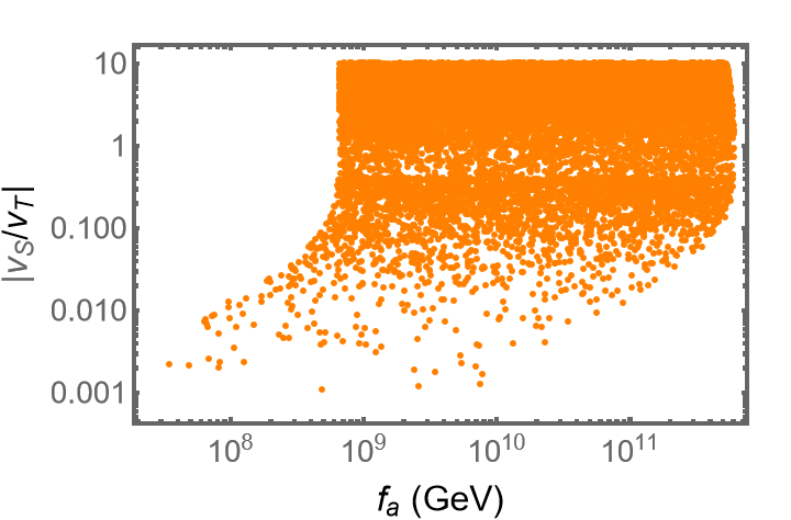
Figure 1: Allowed values of $f_{a}$ as a function of the VEV ratio $v_{S}/v_{T}$. here we have imposed the axion quality constraint on the parameters of the model.

Axion quality constraint: From the gauge quantum numbers of the various fields in the model (see Table I), we find that the leading gravity-induced PQ symmetry breaking term in the scalar potential is

$$V_{\rm gravity}=\frac{\kappa\,e^{i\delta}\,T^{12}\,S^{*}}{(12)!\,M_{\rm Pl}^{9}}+h.c.$$ (12)

This shifts the minimum of the axion potential from $\overline{\theta}=0$ to a finite value. Defining $r\equiv\frac{v_{S}^{2}}{v_{T}^{2}}$ and using the relation $X\simeq v_{T}^{2}v^{2}$, the shift in $\overline{\theta}$ is found to be

$$\overline{\theta}\simeq\left(\frac{\kappa\sin\delta}{(12)!\,2^{11/2}}\right)\left(\frac{f_{a}^{13}}{f_{\pi}^{2}\,m_{\pi}^{2}\,M_{\rm Pl}^{9}}\right)$$

$$\times\frac{(m_{u}+m_{d})^{2}}{m_{u}\,m_{d}}\left(\frac{(1+144r)^{13/2}}{r^{6}}\right)~{}.$$ (13)

The minimum of $\overline{\theta}$ as a function of $r$ occurs for $r=1/12$. Using this, and using $\kappa\sin\delta=1$, $M_{\rm Pl}=1.22\times 10^{19}$ GeV and $m_{u}/m_{d}=0.55$, the maximum value for $f_{a}$ that keeps $|\overline{\theta}|\leq 10^{-10}$ is found to be $f_{a}<4.2\times 10^{11}$ GeV. This can also be seen from Fig. 1, which shows a scatter plot of $f_{a}$ obtained by varying the weak scale VEVs $V_{u,d}$, the angles ($\beta_{u},\,\beta_{d}$) and the high scale VEVs $v_{S,T}$. This upper limit on $f_{a}$ corresponds to a lower bound on the axion mass, $m_{a}\geq 14$ $\mu$eV. In obtaining Fig. 1, we have used the constraints on fermion mass fit which fixes the VEV ratios $|v_{u}/v_{d}|\simeq 70.3$ and $v_{u}^{\prime}/v_{d}^{\prime}\simeq|18.1+3.7i|$ Babu:2020tnf .

Axion couplings and its hybrid nature: To study other phenomenological implications of the model as well to show its hybrid nature, we calculate the couplings of the axion to two photons, electron and the nucleon. For the axion-photon coupling we find

$$g_{a\gamma\gamma}=\frac{\alpha_{em}C_{em}}{2\pi f_{a}}~{}.$$ (14)

Here $C_{em}$=$\frac{8}{3}-1.92$ with the first term arising from triangle diagrams with fermions and the second model-independent term coming from the non-perturbative QCD effects such as $a-\pi^{0}$ mixing Srednicki:1985xd ; Georgi:1986df ; GrillidiCortona:2015jxo ; DiLuzio:2021pxd . This coupling has the same value as in the DFSZ and KSVZ models. The axion coupling to electron and nucleon have the form given in Eq. (5) with the $C_{af}$-factors given by

$$C_{ae} = \frac{24r}{1+144r}K_{e}$$

$$C_{ap} = -0.47+\frac{r}{1+144r}(20.75K_{u}-10.49K_{e})$$

$$C_{an} = -0.02+\frac{r}{1+144r}(19.99K_{e}-9.73K_{u}).$$ (15)

Here we have defined

$$K_{u}=\frac{2{V_{d}}^{2}+\tilde{v}^{2}}{v^{2}},~{}~{}~{}K_{e}=\frac{2{V_{u}}^{2}+\tilde{v}^{2}}{v^{2}}.$$ (16)

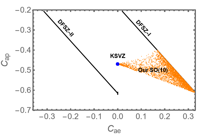
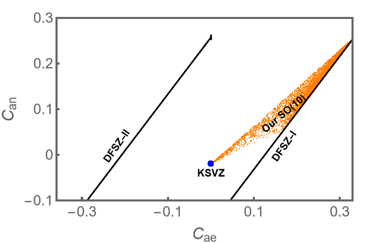
Figure 2: Correlations of axion-proton coupling (top) and axion-neutron coupling (bottom) with the axion-electron coupling in the $SO(10)$ model (yellow dots). Also shown are the values corresponding to KSVZ and DFSZ models.

We now turn to analyzing the model predictions and comparing them with the KSVZ and DFSZ axion models. In Fig. 2, we display the correlation between $C_{ae}$ and $C_{ap}$ (top figure) as well as $C_{ae}$ and $C_{an}$ (bottom figure) as a way to test the model. In obtaining Fig. 2, we have used the values of $|v_{u}/v_{d}|$ and $v_{u}^{\prime}/v_{d}^{\prime}$ obtained from fermion fits quoted above. We find that $K_{e}$ has a range $(1.5-2)$ corresponding to $\tilde{v}=V_{u}$ and $\tilde{v}\ll V_{u}$. The value of $K_{u}$ can be much smaller, with an upper limit of 0.5 (corresponding to $\tilde{v}=V_{u}$). This gives a range $C_{ae}=(0.25-0.33)$ for $r=(0.1-10)$. In the DFSZ-I model the model-dependent couplings of $(u,d,e)$ to the axion are given as $c_{u}^{0}=(1/3)\cos^{2}\beta$, $c_{d}^{0}=c_{e}^{0}=(1/3)\sin^{2}\beta$. The value of $c_{e}^{0}$ changes in DSFZ-II model to $c_{e}^{0}=-(1/3)\cos^{2}\beta$ DiLuzio:2020wdo ; GrillidiCortona:2015jxo .

The blue dots in Fig. 2 are the predictions of the KSVZ model. The black lines are the predictions of the DFSZ-I and DFSZ-II models and the yellow dots are the predictions of our $SO(10)$ model. Depending on where the measured values of these observables lie, our model can be distinguished from the KSVZ and DFSZ models. These model predictions can be tested in various experiments which probe $C_{ae}$ and $C_{ap}/C_{an}$ individually as a function of $m_{a}$. For example, the solar axions are being probed using electron and nuclear interactions and detected by atomic and nuclear absorptions, respectively XENON:2020rca ; PandaX:2017ock ; Lella:2023bfb ; Bhusal:2020bvx . Beam dump experiments are also able to probe these couplings separately using electron scattering and nuclear absorption CCM:2021jmk ; Capozzi:2023ffu ; Waites:2022tov . A positive signal in axion-photon conversion experiments Sikivie:1983ip ; CAST:2017uph ; ADMX:2019uok ; IAXO:2020wwp ; XENON:2022ltv will determine $f_{a}$, in which case measurement of any one of the couplings $C_{ae},\,C_{ap}$ or $C_{an}$ in beam dump or solar axion searches would test our model.

We note that our model interpolates between the KSVZ and DFSZ-I models as we change the ratio $r=v^{2}_{S}/v^{2}_{T}$, as can be seen from the axion composition of the model in Eq. (8). As $r\rightarrow 0$, axion mostly consists of the field $\eta_{S}$, while in the $r\rightarrow\infty$ limit it mostly consists of $\eta_{T}$. From Eq. (6) it is clear that in the $r\rightarrow 0$ limit the axion couples predominantly to the vector-like quarks in the 10-fermion resembling the KSVZ model, while in the $r\rightarrow\infty$ limit it couples to the SM quarks in the 16-fermions, in analogy to the DFSZ-I model. (The DFSZ-II model is not realized in this $SO(10)$ setup.) This interpolation is also reflected in Fig. 2 and Eqs. (15)-(16). We see that, as $r\rightarrow 0$, the couplings to $e,p$ and $n$ reduce to the KSVZ values, whereas for $r\rightarrow\infty$ they go to DFSZ-I values. This confirms that $r$ is indeed an interpolating parameter and for general $r$, the predictions for the above observables lie in the yellow region of Fig. 2 representing the hybrid nature of our model.

Domain Wall in the $SO(10)$ model: We now address the domain wall issue in our model, which is generically problematic in axion models Sikivie:1982qv . To get the number of domain walls in the $SO(10)\times U(1)_{a}$ model, we employ the prescription given in Ref. Ernst:2018bib :

$$N_{\rm DW}={\rm min~{}integer}\left\{\frac{1}{f_{a}}\sum_{i}n_{i}\,c_{i}\,f_{i},~{}n_{i}\in{\cal Z}\right\}~{}$$ (17)

where $a\equiv\sum_{i}c_{i}\eta_{i}$ with the coefficients $c_{i}$ given in Eq. (8) and the definition of $f_{a}$ given in Eq. (11). In our $SO(10)$ model, since there are seven $\eta_{i}$’s there are seven integer $n_{i}$’s. It is easy to see that $N_{DW}=1$ in the model, obtained by setting $n_{S}=1$ and other $n_{i}$’s to zero. This poses no problem with early universe cosmology Sikivie:1982qv .

Other cosmological issues: First we note that, with $f_{a}\leq 4.2\times 10^{11}$ GeV, the axion can serve as dark matter of the universe with the correct relic density Borsanyi:2016ksw . This assumes that the PQ symmetry breaking occurs after inflation ends, in which case there is no contradiction with current limits on iso-curvature fluctuations.

The three singlet fermions $N_{1,2,3}$ of the model have sub-eV mass arising from Planck suppressed operators. As such, these fields can impact BBN. However, their interactions with the SM particles are via the exchange of the $U(1)_{a}$ gauge boson, which has mass of order $v_{a}\sim 10^{12}$ GeV. As a result, the $N_{i}$’s go out of equilibrium at $T_{*}\simeq v_{a}(v_{a}/M_{\rm Pl})^{1/3}\simeq 10^{9}$ GeV. Therefore their contribution to energy density at the epoch of BBN is small with $\Delta N_{eff}\simeq 0.13$. This is in agreement with current CMB observations, but will be tested in planned next generation CMB experiments.

The singlet $\chi$ in our model has a mass of order TeV, and since its interactions with the SM particles are very weak, it can potentially overclose the universe. A simple resolution of this is to give it a large mass, of order the PQ breaking scale, by introducing an $SO(10)$ singlet fermion $N_{0}$ with zero $U(1)_{a}$ charge, which does not affect the anomaly cancellation or any other property of the model. This fermion will have a Yukawa coupling of the type $\chi N_{0}S^{*}$, which would give it a Dirac mass of order $10^{12}$ GeV. Now, a dimension-six four-fermion operator of the form $\chi N_{1}N_{1}N_{1}/M^{2}_{\rm Pl}$ is allowed in the Lagrangian. Since the $N_{1}$ is light, the decay $\chi\rightarrow 3N_{1}$ will proceed with a width given by $\Gamma_{\chi}\sim(m^{5}_{\chi}/M_{\rm Pl}^{4})/192\pi^{3}\sim 10^{-20}$ GeV. Since the $\chi$ fermion decays when $\Gamma_{\chi}$ equals the Hubble expansion rate, the decay temperature can be estimated to be of order GeV, which will leave the successes of BBN unaffected.

In conclusion, we have constructed a minimal and fully realistic $SO(10)$ model, a first of its kind, for a high quality axion that allows the maximum PQ scale of $4\times 10^{11}$ GeV with no domain wall problem. The axion can be the dark matter of the universe. The model has the unique property that it interpolates between the popular KSVZ and DFSZ models and predicts the nucleon and electron couplings of the axion to be different from other models, making the model testable.

Acknowledgements: KB and RNM wish to thank the Mitchell Institute for Fundamental Physics & Astronomy at Texas A&M university for its warm hospitality during the Mitchell workshop in 2023 where this work was initiated. The work of KSB is supported by the U.S. Department of Energy grant No. DE-SC0016013, and that of BD by DOE grant No. DE-SC0010813.

Appendix A Identifying the axion field

We parametrize the neutral Higgs fields, freezing their radial modes, as

$$H_{u}^{10}=\frac{v_{u}e^{i\alpha_{u}}}{\sqrt{2}}e^{i\frac{\eta_{u}}{v_{u}}},~{}~{}~{}H_{u}^{\overline{126}}=\frac{v_{u}^{\prime}e^{i\alpha_{u}^{\prime}}}{\sqrt{2}}e^{i\frac{\eta_{u}^{\prime}}{v_{u}^{\prime}}},~{}~{}~{}H_{d}^{10}=\frac{v_{d}e^{i\alpha_{d}}}{\sqrt{2}}e^{i\frac{\eta_{d}}{v_{d}}},~{}~{}~{}H_{d}^{\overline{126}}=\frac{v_{d}^{\prime}e^{i\alpha_{d}^{\prime}}}{\sqrt{2}}e^{i\frac{\eta_{d}^{\prime}}{v_{d}^{\prime}}},$$ (18)

$$\tilde{H}^{10}=\frac{\tilde{v}e^{i\tilde{\alpha}}}{\sqrt{2}}e^{i\frac{\tilde{\eta}}{\tilde{v}}},~{}~{}~{}\Delta_{R}^{\overline{126}}=\frac{v_{R}e^{i\alpha_{R}}}{\sqrt{2}}e^{i\frac{\eta_{R}}{v_{R}}},~{}~{}~{}S=\frac{v_{S}e^{i\alpha_{S}}}{\sqrt{2}}e^{i\frac{\eta_{S}}{v_{S}}},~{}~{}~{}T=\frac{v_{T}e^{i\alpha_{T}}}{\sqrt{2}}e^{i\frac{\eta_{T}}{v_{T}}}~{}.$$

Here the $H$-fields are neutral components of Higgs doubelts of the SM, with $\tilde{H}^{10}$ being the up-type Higgs doublet from the real 10-plet $H^{\prime}$, while the others are SM singlet fields. All parameters $(v_{j},\,\alpha_{j})$ as well as the fields $\eta_{j}(x)$ are real in Eq. (18). The axion field should be orthogonal to the three Goldstone bosons eaten up by the massive gauge fields $(Z_{\mu},\,X_{\mu},\,V^{(a)}_{\mu})$, where $X_{\mu}$ corresponds to the gauge boson of $U(1)_{X}$ with $SO(10)\supset SU(5)\times U(1)_{X}$ and $V_{\mu}^{(a)}$ is the vector boson associated with the $U(1)_{a}$. Furthermore, the axion is orthogonal to the four massive pseudoscalar fields. The Goldstone fields are identified as:

$$G_{Z} = N_{Z}(v_{u}\,\eta_{u}+v^{\prime}_{u}\,\eta^{\prime}_{u}-v_{d}\,\eta_{d}-v^{\prime}_{d}\,\eta^{\prime}_{d}+\tilde{v}\,\tilde{\eta})$$

$$G_{X} = N_{X}(10\,v_{R}\,\eta_{R}+2\,v_{u}\,\eta_{u}+2\,v^{\prime}_{u}\,\eta^{\prime}_{u}-2\,v_{d}\,\eta_{d}-2\,v^{\prime}_{d}\,\eta^{\prime}_{d}+2\,\tilde{v}\,\tilde{\eta})$$

$$G_{a} = N_{a}(-2\,v_{R}\,\eta_{R}+v_{T}\,\eta_{T}+12\,v_{S}\,\eta_{S}-2\,v_{u}\,\eta_{u}-2\,v^{\prime}_{u}\,\eta^{\prime}_{u}-2\,v_{d}\,\eta_{d}-2\,v^{\prime}_{d}\,\eta^{\prime}_{d})~{}.$$ (19)

The massive pseudoscalar fields are identified from the Higgs potential given in Eq. (7) as:

$${\cal A}_{1} = N_{1}\left[\frac{\eta_{u}}{v_{u}}-\frac{\eta^{\prime}_{u}}{v^{\prime}_{u}}\right]$$

$${\cal A}_{2} = N_{2}\left[\frac{\eta_{d}}{v_{d}}-\frac{\eta^{\prime}_{d}}{v^{\prime}_{d}}\right]$$

$${\cal A}_{3} = N_{3}\left[2\frac{\eta_{T}}{v_{T}}+\frac{\eta_{u}}{v_{u}}-\frac{\tilde{\eta}}{\tilde{v}}\right]$$

$${\cal A}_{4} = N_{4}\left[2\frac{\eta_{T}}{v_{T}}+\frac{\eta_{d}}{v_{d}}+\frac{\tilde{\eta}}{\tilde{v}}\right]~{}.$$ (20)

Here the $N_{i}$-factors are normalization coefficients. The axion field is now readilty identified and is given in Eq. (8).

References

- (1) R. J. Crewther, P. Di Vecchia, G. Veneziano, and E. Witten, “Chiral Estimate of the Electric Dipole Moment of the Neutron in Quantum Chromodynamics,” Phys. Lett. B 88 (1979) 123. [Erratum: Phys.Lett.B 91, 487 (1980)].
- (2) C. Abel et al., “Measurement of the Permanent Electric Dipole Moment of the Neutron,” Phys. Rev. Lett. 124 no. 8, (2020) 081803, arXiv:2001.11966 [hep-ex].
- (3) R. D. Peccei and H. R. Quinn, “CP Conservation in the Presence of Instantons,” Phys. Rev. Lett. 38 (1977) 1440–1443.
- (4) S. Weinberg, “A New Light Boson?,” Phys. Rev. Lett. 40 (1978) 223–226.
- (5) F. Wilczek, “Problem of Strong and Invariance in the Presence of Instantons,” Phys. Rev. Lett. 40 (1978) 279–282.
- (6) P. Di Vecchia and G. Veneziano, “Chiral Dynamics in the Large n Limit,” Nucl. Phys. B 171 (1980) 253–272.
- (7) J. E. Kim, “Weak Interaction Singlet and Strong CP Invariance,” Phys. Rev. Lett. 43 (1979) 103.
- (8) M. A. Shifman, A. I. Vainshtein, and V. I. Zakharov, “Can Confinement Ensure Natural CP Invariance of Strong Interactions?,” Nucl. Phys. B 166 (1980) 493–506.
- (9) M. Dine, W. Fischler, and M. Srednicki, “A Simple Solution to the Strong CP Problem with a Harmless Axion,” Phys. Lett. B 104 (1981) 199–202.
- (10) A. R. Zhitnitsky, “On Possible Suppression of the Axion Hadron Interactions. (In Russian),” Sov. J. Nucl. Phys. 31 (1980) 260.
- (11) L. Di Luzio, M. Giannotti, E. Nardi, and L. Visinelli, “The landscape of QCD axion models,” Phys. Rept. 870 (2020) 1–117, arXiv:2003.01100 [hep-ph].
- (12) G. Grilli di Cortona, E. Hardy, J. Pardo Vega, and G. Villadoro, “The QCD axion, precisely,” JHEP 01 (2016) 034, arXiv:1511.02867 [hep-ph].
- (13) M. Kamionkowski and J. March-Russell, “Planck scale physics and the Peccei-Quinn mechanism,” Phys. Lett. B 282 (1992) 137–141, arXiv:hep-th/9202003.
- (14) R. Holman, S. D. H. Hsu, T. W. Kephart, E. W. Kolb, R. Watkins, and L. M. Widrow, “Solutions to the strong CP problem in a world with gravity,” Phys. Lett. B 282 (1992) 132–136, arXiv:hep-ph/9203206.
- (15) S. M. Barr and D. Seckel, “Planck scale corrections to axion models,” Phys. Rev. D 46 (1992) 539–549.
- (16) S. Ghigna, M. Lusignoli, and M. Roncadelli, “Instability of the invisible axion,” Phys. Lett. B 283 (1992) 278–281.
- (17) Y.-C. Qiu, J.-W. Wang, and T. T. Yanagida, “High-Quality Axions in a Class of Chiral U(1) Gauge Theories,” Phys. Rev. Lett. 131 no. 7, (2023) 071802, arXiv:2301.02345 [hep-ph].
- (18) L. Di Luzio, “Accidental SO(10) axion from gauged flavour,” JHEP 11 (2020) 074, arXiv:2008.09119 [hep-ph].
- (19) M. Ardu, L. Di Luzio, G. Landini, A. Strumia, D. Teresi, and J.-W. Wang, “Axion quality from the (anti)symmetric of SU(),” JHEP 11 (2020) 090, arXiv:2007.12663 [hep-ph].
- (20) L. Randall, “Composite axion models and Planck scale physics,” Phys. Lett. B 284 (1992) 77–80.
- (21) B. Lillard and T. M. P. Tait, “A High Quality Composite Axion,” JHEP 11 (2018) 199, arXiv:1811.03089 [hep-ph].
- (22) L. Vecchi, “Axion quality straight from the GUT,” Eur. Phys. J. C 81 no. 10, (2021) 938, arXiv:2106.15224 [hep-ph].
- (23) H.-S. Lee and W. Yin, “Peccei-Quinn symmetry from a hidden gauge group structure,” Phys. Rev. D 99 no. 1, (2019) 015041, arXiv:1811.04039 [hep-ph].
- (24) P. Cox, T. Gherghetta, and A. Paul, “A common origin for the QCD axion and sterile neutrinos from SU(5) strong dynamics,” JHEP 12 (2023) 180, arXiv:2310.08557 [hep-ph].
- (25) P. Cox, T. Gherghetta, and M. D. Nguyen, “Light sterile neutrinos and a high-quality axion from a holographic Peccei-Quinn mechanism,” Phys. Rev. D 105 no. 5, (2022) 055011, arXiv:2107.14018 [hep-ph].
- (26) Y. Nakai and M. Suzuki, “Axion Quality from Superconformal Dynamics,” Phys. Lett. B 816 (2021) 136239, arXiv:2102.01329 [hep-ph].
- (27) K. S. Babu, I. Gogoladze, and K. Wang, “Stabilizing the axion by discrete gauge symmetries,” Phys. Lett. B 560 (2003) 214–222, arXiv:hep-ph/0212339.
- (28) Z. Berezhiani, L. Gianfagna, and M. Giannotti, “Strong CP problem and mirror world: The Weinberg-Wilczek axion revisited,” Phys. Lett. B 500 (2001) 286–296, arXiv:hep-ph/0009290.
- (29) A. Hook, S. Kumar, Z. Liu, and R. Sundrum, “High Quality QCD Axion and the LHC,” Phys. Rev. Lett. 124 no. 22, (2020) 221801, arXiv:1911.12364 [hep-ph].
- (30) A. Hook, “Solving the Hierarchy Problem Discretely,” Phys. Rev. Lett. 120 no. 26, (2018) 261802, arXiv:1802.10093 [hep-ph].
- (31) A. Banerjee, J. Eby, and G. Perez, “From axion quality and naturalness problems to a high-quality ZN QCD relaxion,” Phys. Rev. D 107 no. 11, (2023) 115011, arXiv:2210.05690 [hep-ph].
- (32) K.-w. Choi, “A QCD axion from higher dimensional gauge field,” Phys. Rev. Lett. 92 (2004) 101602, arXiv:hep-ph/0308024.
- (33) P. Svrcek and E. Witten, “Axions In String Theory,” JHEP 06 (2006) 051, arXiv:hep-th/0605206.
- (34) K. S. Babu and R. N. Mohapatra, “Predictive neutrino spectrum in minimal SO(10) grand unification,” Phys. Rev. Lett. 70 (1993) 2845–2848, arXiv:hep-ph/9209215.
- (35) B. Bajc, G. Senjanovic, and F. Vissani, “How neutrino and charged fermion masses are connected within minimal supersymmetric SO(10),” PoS HEP2001 (2001) 198, arXiv:hep-ph/0110310.
- (36) T. Fukuyama and N. Okada, “Neutrino oscillation data versus minimal supersymmetric SO(10) model,” JHEP 11 (2002) 011, arXiv:hep-ph/0205066.
- (37) B. Bajc, G. Senjanovic, and F. Vissani, “b - tau unification and large atmospheric mixing: A Case for noncanonical seesaw,” Phys. Rev. Lett. 90 (2003) 051802, arXiv:hep-ph/0210207.
- (38) H. S. Goh, R. N. Mohapatra, and S.-P. Ng, “Minimal SUSY SO(10), b tau unification and large neutrino mixings,” Phys. Lett. B 570 (2003) 215–221, arXiv:hep-ph/0303055.
- (39) H. S. Goh, R. N. Mohapatra, and S.-P. Ng, “Minimal SUSY SO(10) model and predictions for neutrino mixings and leptonic CP violation,” Phys. Rev. D 68 (2003) 115008, arXiv:hep-ph/0308197.
- (40) K. S. Babu and C. Macesanu, “Neutrino masses and mixings in a minimal SO(10) model,” Phys. Rev. D 72 (2005) 115003, arXiv:hep-ph/0505200.
- (41) S. Bertolini, M. Frigerio, and M. Malinsky, “Fermion masses in SUSY SO(10) with type II seesaw: A Non-minimal predictive scenario,” Phys. Rev. D 70 (2004) 095002, arXiv:hep-ph/0406117.
- (42) S. Bertolini and M. Malinsky, “On CP violation in minimal renormalizable SUSY SO(10) and beyond,” Phys. Rev. D 72 (2005) 055021, arXiv:hep-ph/0504241.
- (43) S. Bertolini, T. Schwetz, and M. Malinsky, “Fermion masses and mixings in SO(10) models and the neutrino challenge to SUSY GUTs,” Phys. Rev. D 73 (2006) 115012, arXiv:hep-ph/0605006.
- (44) B. Bajc, I. Dorsner, and M. Nemevsek, “Minimal SO(10) splits supersymmetry,” JHEP 11 (2008) 007, arXiv:0809.1069 [hep-ph].
- (45) A. S. Joshipura and K. M. Patel, “Fermion Masses in SO(10) Models,” Phys. Rev. D 83 (2011) 095002, arXiv:1102.5148 [hep-ph].
- (46) A. Dueck and W. Rodejohann, “Fits to SO(10) Grand Unified Models,” JHEP 09 (2013) 024, arXiv:1306.4468 [hep-ph].
- (47) G. Altarelli and D. Meloni, “A non supersymmetric SO(10) grand unified model for all the physics below ,” JHEP 08 (2013) 021, arXiv:1305.1001 [hep-ph].
- (48) T. Fukuyama, K. Ichikawa, and Y. Mimura, “Revisiting fermion mass and mixing fits in the minimal SUSY GUT,” Phys. Rev. D 94 no. 7, (2016) 075018, arXiv:1508.07078 [hep-ph].
- (49) K. S. Babu, B. Bajc, and S. Saad, “Resurrecting Minimal Yukawa Sector of SUSY SO(10),” JHEP 10 (2018) 135, arXiv:1805.10631 [hep-ph].
- (50) T. Ohlsson and M. Pernow, “Fits to Non-Supersymmetric SO(10) Models with Type I and II Seesaw Mechanisms Using Renormalization Group Evolution,” JHEP 06 (2019) 085, arXiv:1903.08241 [hep-ph].
- (51) K. S. Babu and S. Saad, “Flavor Hierarchies from Clockwork in SO(10) GUT,” Phys. Rev. D 103 no. 1, (2021) 015009, arXiv:2007.16085 [hep-ph].
- (52) S. Bertolini, L. Di Luzio, and M. Malinsky, “Intermediate mass scales in the non-supersymmetric SO(10) grand unification: A Reappraisal,” Phys. Rev. D 80 (2009) 015013, arXiv:0903.4049 [hep-ph].
- (53) K. S. Babu, B. Bajc, and S. Saad, “Yukawa Sector of Minimal SO(10) Unification,” JHEP 02 (2017) 136, arXiv:1612.04329 [hep-ph].
- (54) K. S. Babu and S. Khan, “Minimal nonsupersymmetric model: Gauge coupling unification, proton decay, and fermion masses,” Phys. Rev. D 92 no. 7, (2015) 075018, arXiv:1507.06712 [hep-ph].
- (55) K. Jarkovská, M. Malinský, T. Mede, and V. Susič, “Quantum nature of the minimal potentially realistic SO(10) Higgs model,” Phys. Rev. D 105 no. 9, (2022) 095003, arXiv:2109.06784 [hep-ph].
- (56) M. Srednicki, “Axion Couplings to Matter. 1. CP Conserving Parts,” Nucl. Phys. B 260 (1985) 689–700.
- (57) H. Georgi, D. B. Kaplan, and L. Randall, “Manifesting the Invisible Axion at Low-energies,” Phys. Lett. B 169 (1986) 73–78.
- (58) L. Di Luzio, B. Gavela, P. Quilez, and A. Ringwald, “An even lighter QCD axion,” JHEP 05 (2021) 184, arXiv:2102.00012 [hep-ph].
- (59) XENON Collaboration, E. Aprile et al., “Excess electronic recoil events in XENON1T,” Phys. Rev. D 102 no. 7, (2020) 072004, arXiv:2006.09721 [hep-ex].
- (60) PandaX Collaboration, C. Fu et al., “Limits on Axion Couplings from the First 80 Days of Data of the PandaX-II Experiment,” Phys. Rev. Lett. 119 no. 18, (2017) 181806, arXiv:1707.07921 [hep-ex].
- (61) A. Lella, P. Carenza, G. Co’, G. Lucente, M. Giannotti, A. Mirizzi, and T. Rauscher, “Getting the most on supernova axions,” Phys. Rev. D 109 no. 2, (2024) 023001, arXiv:2306.01048 [hep-ph].
- (62) A. Bhusal, N. Houston, and T. Li, “Searching for Solar Axions Using Data from the Sudbury Neutrino Observatory,” Phys. Rev. Lett. 126 no. 9, (2021) 091601, arXiv:2004.02733 [hep-ph].
- (63) CCM Collaboration, A. A. Aguilar-Arevalo et al., “Prospects for detecting axionlike particles at the Coherent CAPTAIN-Mills experiment,” Phys. Rev. D 107 no. 9, (2023) 095036, arXiv:2112.09979 [hep-ph].
- (64) F. Capozzi, B. Dutta, G. Gurung, W. Jang, I. M. Shoemaker, A. Thompson, and J. Yu, “New constraints on ALP couplings to electrons and photons from ArgoNeuT and the MiniBooNE beam dump,” Phys. Rev. D 108 no. 7, (2023) 075019, arXiv:2307.03878 [hep-ph].
- (65) L. Waites, A. Thompson, A. Bungau, J. M. Conrad, B. Dutta, W.-C. Huang, D. Kim, M. Shaevitz, and J. Spitz, “Axionlike particle production at beam dump experiments with distinct nuclear excitation lines,” Phys. Rev. D 107 no. 9, (2023) 095010, arXiv:2207.13659 [hep-ph].
- (66) P. Sikivie, “Experimental Tests of the Invisible Axion,” Phys. Rev. Lett. 51 (1983) 1415–1417. [Erratum: Phys.Rev.Lett. 52, 695 (1984)].
- (67) CAST Collaboration, V. Anastassopoulos et al., “New CAST Limit on the Axion-Photon Interaction,” Nature Phys. 13 (2017) 584–590, arXiv:1705.02290 [hep-ex].
- (68) ADMX Collaboration, T. Braine et al., “Extended Search for the Invisible Axion with the Axion Dark Matter Experiment,” Phys. Rev. Lett. 124 no. 10, (2020) 101303, arXiv:1910.08638 [hep-ex].
- (69) IAXO Collaboration, A. Abeln et al., “Conceptual design of BabyIAXO, the intermediate stage towards the International Axion Observatory,” JHEP 05 (2021) 137, arXiv:2010.12076 [physics.ins-det].
- (70) XENON Collaboration, E. Aprile et al., “Search for New Physics in Electronic Recoil Data from XENONnT,” Phys. Rev. Lett. 129 no. 16, (2022) 161805, arXiv:2207.11330 [hep-ex].
- (71) P. Sikivie, “Of Axions, Domain Walls and the Early Universe,” Phys. Rev. Lett. 48 (1982) 1156–1159.
- (72) A. Ernst, A. Ringwald, and C. Tamarit, “Axion Predictions in Models,” JHEP 02 (2018) 103, arXiv:1801.04906 [hep-ph].
- (73) S. Borsanyi et al., “Calculation of the axion mass based on high-temperature lattice quantum chromodynamics,” Nature 539 no. 7627, (2016) 69–71, arXiv:1606.07494 [hep-lat].