Exact analytic toolbox for quantum dynamics with tunable noise strength

Abstract

We introduce a framework that allows for the exact analytic treatment of quantum dynamics subject to coherent noise. The noise is modeled via unitary evolution under a Hamiltonian drawn from a random-matrix ensemble for arbitrary Hilbert-space dimension $N$. While the methods we develop apply to generic such ensembles with a notion of rotation invariance, we focus largely on the Gaussian unitary ensemble (GUE). Averaging over the ensemble of “noisy” Hamiltonians produces an effective quantum channel, the properties of which are analytically calculable and determined by the spectral form factors of the relevant ensemble. We compute spectral form factors of the GUE exactly for any finite $N$, along with the corresponding GUE quantum channel, and its variance. Key advantages of our approach include the ability to access exact analytic results for any $N$ and the ability to tune to the noise-free limit (in contrast, e.g., to the Haar ensemble), and analytic access to moments beyond the variance. We also highlight some unusual features of the GUE channel, including the nonmonotonicity of the coefficients of various operators as a function of noise strength and the failure to saturate the Haar-random limit, even with infinite noise strength.

1 Introduction

The advent of quantum hardware with experimentally controllable qubits has led to significant interest in quantum dynamics. Of particular interest is how these synthetic quantum systems can be used to realize new capabilities for near-term technologies. These efforts include identifying quantum algorithms that outperform classical analogues [1, 2, 3], quantum error correction (QEC) for the storage of logical qubits [4, 5, 6, 7, 8, 9, 10, 11, 12, 13], the preparation of many-body resource states [3, 14, 15, 16, 17], controlled simulations of quantum dynamics of real materials [18], learning about unknown quantum states and processes [19, 20, 21], developing precision sensors for, e.g., metrology [22, 23], and even playing nonlocal quantum games [24, 25, 26, 27, 28].

While quantum technologies can realize significant advantages over their classical analogues (e.g., quantum computation), they are generally far more sensitive to sources of error [1, 2, 3]. Accordingly, a crucial area of research is the development of strategies for mitigating and correcting for such errors. In the context of stabilizer QEC [4, 5, 6, 7, 8, 9, 10, 11, 12, 13], e.g., it is often the case that arbitrary local errors can be corrected via measurements and outcome-dependent feedback before they can proliferate and produce a logical error [3, 29]. Beyond this setting, the effects of noise on quantum systems—and strategies for their mitigation—must be considered on a case-by-case basis.

However, outside of the context of stabilizer QEC [4, 5, 6, 7, 8, 9, 10, 11, 12, 13], tools for the analytical treatment of noisy quantum dynamics are generally lacking. While the Lindblad description [30, 31, 3, 32, 33, 29] of open quantum systems describes decohering effects due to interaction of a quantum system with a Markovian environment, the coherent sources of error of interest herein are generally modeled using noisy numerical simulations. Accordingly, we expect the framework we present herein to be useful to the description of dynamics on the noisy intermediate-scale quantum (NISQ) devices presently available.

In this work, we present an analytical toolbox for describing quantum dynamics in the presence of coherent sources of noise with tunable strength. The noisy channel may act on a system of interest, subsets thereof, or the combination of the system and “environmental” degrees of freedom; symmetries and/or constraints may be included using projectors [34, 35, 36]. Exact results are furnished by drawing the unitary evolution operator from ensembles common in random matrix theory (RMT) [37, 38, 39, 40, 41, 42, 43]. In particular, our results apply to noisy evolution generated by random $N\times N$ Hamiltonians $G$ drawn from an ensemble $\mathcal{E}$ whose probability distribution function (PDF) $P_{\mathcal{E}}(G)$ is rotation invariant—i.e., $P_{\mathcal{E}}(UGU^{\dagger})=P_{\mathcal{E}}(G)$ for all $U$ belonging to some matrix group $\mathsf{R}$. The noise strength is captured either by the duration $t$ of time evolution generated by $G$ or, equivalently, the standard deviation $\sigma$ of the distribution $P_{\mathcal{E}}(G)$.

For concreteness, we explicitly consider Hamiltonians $G$ drawn from the Gaussian unitary ensemble (GUE) [38, 43, 42, 41, 39, 40]. We derive an expression for the average evolution of any operator $A$ or density matrix in Sec. 3; the result contains two $t$-dependent terms, proportional to $A$ and $\operatorname*{tr}(A)\mathds{1}$, respectively, effectively realizing a depolarizing channel [3] whose strength depends only on $\smash{\sigma^{2}t^{2}}$, where $\smash{\sigma^{2}}$ is the variance of matrix elements of $G$. This time dependence is related to the two-point spectral form factor (SFF) $\mathcal{R}_{2}(t)$ [44, 45, 46, 47, 34, 35, 36], a standard diagnostic of spectral rigidity (i.e., level repulsion) in quantum systems, and a common diagnostic in the field of quantum chaos [44, 45, 46, 47, 34, 35, 36, 48]. We compute the two-point SFF for the GUE exactly for any finite $N$, correcting typos that appear in Ref. 49. We also compute the variance of the noisy channel, which can be used to diagnose, e.g., typicality of the average. We also describe the evaluation of arbitrary cumulants, where the $k$th cumulant depends on the $2k$-point and lower SFFs; in Sec. 4 we compute exactly the first few SFFs for the GUE for arbitrary Hilbert-space dimension $N$, and also detail how to compute all SFFs. We expect these results to be relevant to quantum chaos [50, 44, 46, 45, 47, 34, 35, 36, 51] and even the study of black holes [46, 41, 45, 49, 52]. For comparison, we also consider the unitary evolution of a single qubit in Sec. 2, finding exact results without the need to average over an ensemble. Although we primarily use this result to benchmark calculations for the more general $N\!\times\!N$ case, it may also be relevant to developing strategies for error correction on NISQ devices.

Our results also reveal unexpected phenomenology. First, the fidelity of the depolarizing channel is nonmonotonic in the noise strength. Consequently the “typicality” of the average channel (compared to typical instances of a noisy unitary) can be improved to some extent by increasing the strength of the noise. Second, we observe that the “strong-noise” limit of the GUE channel does not saturate the Haar-random limit, which leads to the maximally mixed state. We explain these counterintuitive results below, using the machinery of spectral form factors. We also comment that the existence of such unexpected phenomena even in the simple case of the GUE suggests that even more interesting behaviors may emerge in the context of noise drawn from more structured ensembles.

2 Noisy single-qubit channels

We begin by considering arbitrary unitary operations on single qubits. In addition to providing a useful warm up to the more general noisy unitaries considered in Sec. 3, the single-qubit example admits exact solutions even without averaging over a particular ensemble of unitary operators, providing a useful benchmark for the more general case $N\geq 2$.

We first note that a single-qubit observable (or density matrix) $A$ can be decomposed onto the Pauli operators according to

$$A=\frac{1}{2}\operatorname*{tr}(A)\hskip 1.13809pt\mathds{1}+\boldsymbol{a}\cdot\boldsymbol{\sigma}\,,~{}$$ (1)

where the three-vector $\boldsymbol{a}$ has coefficients $a_{\nu}=\operatorname*{tr}(A\hskip 1.13809pt\sigma^{\nu})/2$, and $\boldsymbol{\sigma}=(\sigma^{x},\sigma^{y},\sigma^{z})$ is a three-vector of Pauli matrices.

Suppose that $A$ (1) evolves in the Heisenberg picture under some single-qubit Hamiltonian $G$ of the form (1), i.e.,

$$A_{\boldsymbol{g}}(t)=\mathrm{e}^{\mathrm{i}t\boldsymbol{g}\cdot\boldsymbol{\sigma}}A\hskip 1.13809pt\mathrm{e}^{-\mathrm{i}t\boldsymbol{g}\cdot\boldsymbol{\sigma}},~{}~{}$$ (2)

where the part of $G$ proportional to the identity acts trivially, and to capture the Schrödinger evolution of density matrices, one need only replace $t\to-t$. Using Euler’s formula for quaternions, the unitary evolution operator can be written

$$U_{G}(t)=\mathrm{e}^{-\mathrm{i}t\boldsymbol{g}\cdot\boldsymbol{\sigma}}=\cos(gt)\mathds{1}-\mathrm{i}\sin(gt)\hskip 1.13809pt\hat{\boldsymbol{g}}\cdot\boldsymbol{\sigma}\,,~{}~{}$$ (3)

where $g\coloneq\lvert\boldsymbol{g}\rvert$ is the magnitude of $\boldsymbol{g}$ and $\hat{\boldsymbol{g}}\equiv\boldsymbol{g}/g$ is the associated unit vector. Using (3) and various properties of the Pauli matrices, we can rewrite $A_{\boldsymbol{g}}(t)$ (2) as

$$A_{\boldsymbol{g}}(t) =\frac{\operatorname*{tr}(A)}{2}\mathds{1}+\cos(2gt)\hskip 1.13809pt\boldsymbol{a}\cdot\boldsymbol{\sigma}-\frac{\sin(2gt)}{g}(\boldsymbol{g}\times\boldsymbol{a})\cdot\boldsymbol{\sigma}$$

$$\quad+\frac{2\sin^{2}(gt)}{g^{2}}(\boldsymbol{g}\cdot\boldsymbol{a})(\boldsymbol{g}\cdot\boldsymbol{\sigma})\,,~{}$$ (4)

which is exact for any Hermitian $A$ and $G$ and any time $t$.

We are primarily interested in the average of the unitary channel (2) over an RMT ensemble $\mathcal{E}$, captured by

$$\operatorname{avg}(A,t)=\operatorname{\mathbb{E}}_{\mathcal{E}}[A(t)]\coloneq\txintop\nolimits\mathrm{d}^{3}\boldsymbol{g}\,A_{\boldsymbol{g}}(t)\,P_{\mathcal{E}}(\boldsymbol{g})\,,~{}~{}$$ (5)

where $P_{\mathcal{E}}(\boldsymbol{g})$ is the probability density function (PDF) for $G=\boldsymbol{g}\cdot\boldsymbol{\sigma}\in\mathcal{E}$. Note that the trace part of $G$ is irrelevant to the channel (2). It is also straightforward to show that the map $A\mapsto\langle A(t)\rangle$ (5) is completely positive and trace preserving (CPTP), and thus a valid quantum channel [3].

In particular, we restrict to the GUE [38, 43, 42, 41, 39, 40], which we review for completeness in App. A. In the case of a single-qubit system, the components $g_{0}=\operatorname*{tr}(G)/2$ and the three Pauli components $\boldsymbol{g}$ (1) are real valued and drawn from the normal distribution $\mathcal{N}_{\mathbb{R}}(0,\sigma^{2}/2)$. Ignoring the trace component $g_{0}$, as it does not contribute to the unitary channel (2), we find that

$$P_{\text{GUE}}(\boldsymbol{g},\sigma)=\frac{1}{\pi^{3/2}\,\sigma^{3}}\mathrm{e}^{-\boldsymbol{g}^{2}/\sigma^{2}}\,,~{}~{}$$ (6)

which follows from the general relation for $N\!\times\!N$ matrices (A.67) in App. A. Using the PDF (6), the average of the unitary channel $A_{\boldsymbol{g}}(t)$ (2) over the GUE leads to

$$\operatorname{avg}(A,t)=\frac{1}{2}\operatorname*{tr}(A)\mathds{1}+h(\sigma t)\,\boldsymbol{a}\cdot\boldsymbol{\sigma}\,,~{}~{}$$ (7)

where we have implicitly defined the function $h(z)$. Importantly, we note that the variance $\sigma$ only appears in the product $\sigma t$; without loss of generality, we fix $\sigma=1/\sqrt{2}$ in the remainder (see App. A for details). To facilitate comparison to results for $N>2$, we rewrite the GUE-averaged channel $\langle A_{\boldsymbol{g}}(t)\rangle$ (7) as

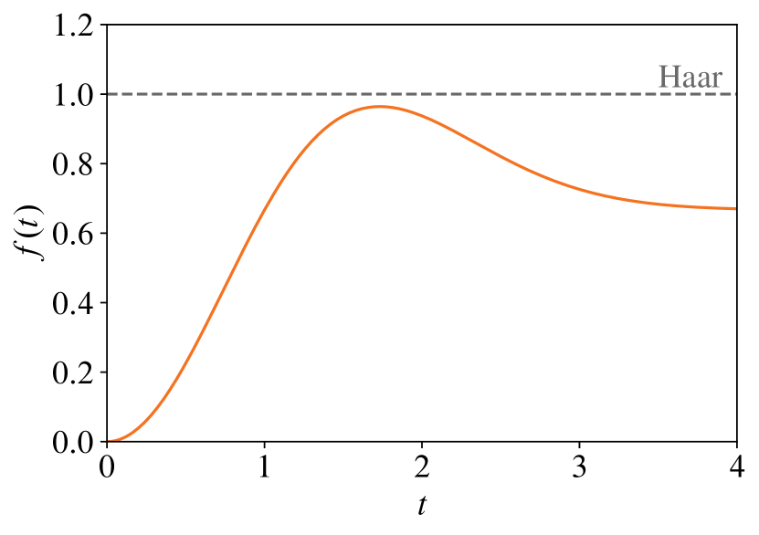
Figure 1: The amplitude $f(t)$ of the term $\operatorname*{tr}(A)\mathds{1}/2$ in the GUE-averaged single-qubit channel $\langle A_{\boldsymbol{g}}(t)\rangle$ (8). For comparison, the dashed line indicates the Haar-random value $f(t)=1$, which is never realized by $\langle A_{\boldsymbol{g}}(t)\rangle$. For $t\gtrsim 4$, $f(t)$ saturates to $2/3$. + AI.

$$\operatorname{avg}(A,t) =\left[1-f(t)\right]A+f(t)\frac{\operatorname*{tr}(A)}{2}\hskip 1.13809pt\mathds{1}\,.~{}$$ (8)

which is parameterized by the single function $f(t)$, defined by

$$f(t)\coloneq\frac{2}{3}\left[1-\mathrm{e}^{-t^{2}/2}\left(1-t^{2}\right)\right]\,,~{}~{}$$ (9)

for qubits and for the choice $\sigma=1/\sqrt{2}$ that we consider herein. In Fig. 1, we plot the amplitude $f(t)$ that appears in the average channel (8). We note that $f(t)$ is nonmonotonic in $t$ and never saturates the Haar-random limit $f(t)=1$. In Sec. 3.2, we generalize $f(t)$ (9) to arbitrary $N\geq 2$.

When applied to density matrices $\rho$, the GUE-averaged channel $\rho\mapsto\langle\rho_{\boldsymbol{g}}(t)\rangle$ (8) realizes a depolarizing channel [3] with a $t$-dependent polarization parameter $p$, i.e.,

$$\Phi_{\text{dp}}(\rho)=(1-p)\rho+\frac{p}{N}\mathds{1}\,,~{}~{}$$ (10)

where $p=f(t)$ (9), and we used the fact that $\operatorname*{tr}(\rho)=1$. At $t=0$, the $\rho$ term has coefficient one, while the $\mathds{1}$ term—corresponding to the maximally mixed state $\rho_{\infty}=\mathds{1}/N$—has coefficient zero. At early times, the coefficient of the maximally mixed state grows like $t^{2}+O(t^{4})$, and is maximized when $t=\sqrt{3}$, where $p_{\text{max}}\approx 0.96$. Importantly, this coefficient is always less than one, meaning that the GUE-averaged channel $\langle\rho_{\boldsymbol{g}}(t)\rangle_{\text{GUE}}$ (8) never realizes the Haar-random limit $\langle\rho_{\boldsymbol{g}}(t)\rangle_{\text{Haar}}=\mathds{1}/2$, due to the additional structure of the GUE compared to the uniform Haar measure [53, 45]. Moreover, $p=f(t)$ is a nonmonotonic function of $t$ (see Fig. 1), which decreases for $t>\sqrt{3}$, saturating to $f(t)=2/3$ for $t\gtrsim 4$. However, we are primarily interested in the limit $t\ll 1$, corresponding to weak noise.

Finally, to probe the extent to which the average GUE channel $\langle A_{\boldsymbol{g}}(t)\rangle$ (8) captures typical values of the time-evolved operator $A_{\boldsymbol{g}}(t)$ (4), we evaluate the variance of $A_{\boldsymbol{g}}(t)$ for $G$ drawn from the GUE [38, 43, 42, 41, 39, 40]. In particular, we define the quantity

$$\operatorname{var}(A,t) \coloneq\operatorname{\mathbb{E}}_{\mathcal{E}}\left[A^{*}_{\boldsymbol{g}}(t)\otimes A^{\vphantom{*}}_{\boldsymbol{g}}(t)\right]-\operatorname{\mathbb{E}}_{\mathcal{E}}\left[A_{\boldsymbol{g}}(t)\right]^{\otimes 2}$$ (11)

$$\;=\frac{7f(t)-3f(2t)-5f(t)^{2}}{5}\left(\boldsymbol{a}\cdot\boldsymbol{\sigma}\right)^{*}\otimes\left(\boldsymbol{a}\cdot\boldsymbol{\sigma}\right)$$

$$~{}~{}+\frac{f(t)+f(2t)}{5}\lvert a\rvert^{2}\sum\limits_{n=1}^{3}\left(\sigma^{n}\right)^{*}\otimes\sigma^{n}\,,~{}~{}$$ (12)

which we use to extract the variance of the individual matrix elements of $A_{\boldsymbol{g}}(t)$ (4). We note that the latter operator can be written in terms of the SWAP operator $\mathcal{S}=\sum_{m,n}\lvert nm\rangle\langle mn\rvert$, which is relevant to the general $N$ case in Sec. 3.3.

We use $\operatorname{var}(A,t)$ (12) to compute the variance of individual matrix elements of $A_{\boldsymbol{g}}(t)$ (2) by evaluating

$$\operatorname{var}(A_{mn},t) \coloneq\langle\lvert A_{mn}(t)\rvert^{2}\rangle-\lvert\langle A_{mn}(t)\rangle\rvert^{2}$$

$$~{}=\operatorname*{tr}\Big{(}\operatorname{var}(A,t)\,\lvert n\rangle\langle m\rvert^{\otimes 2}\Big{)}\,,~{}~{}$$ (13)

so that the two diagonal elements $A_{nn}$ have variance

$$\operatorname{var}(A_{nn},t) =\frac{7f(t)-3f(2t)-5f(t)^{2}}{5}a_{z}^{2}$$

$$~{}+\frac{f(t)+f(2t)}{5}\lvert a\rvert^{2}\,,~{}~{}$$ (14)

while the two off-diagonal elements have variance

$$\operatorname{var}(A_{mn},t) =-\frac{7f(t)-3f(2t)-5f(t)^{2}}{5}a_{z}^{2}$$

$$~{}+\frac{9f(t)-f(2t)-5f(t)^{2}}{5}\lvert a\rvert^{2}\,,~{}~{}$$ (15)

for $m\neq n$. Note that $a_{z}$ and $a=\lvert\boldsymbol{a}\rvert$ refer to the Pauli components of $A$ (1) prior to evolution under the Gaussian Hamiltonian $A\mapsto A_{\boldsymbol{g}}(t)$ (2) and the trace part $a_{0}=\operatorname*{tr}(A)/2$ does not contribute to the variances—intuitively, this is because the identity piece is preserved by the channel (5).

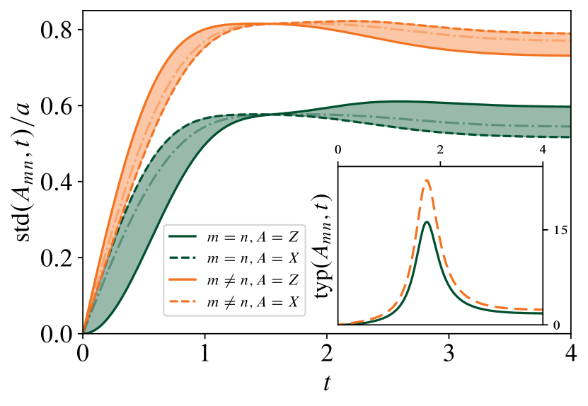
Figure 2: Standard deviation of matrix elements $A_{mn}(t)$ of $A_{G}(t)$ (2) for an initial operator $A=\boldsymbol{a}\cdot\boldsymbol{\sigma}$, in units of $a=\lvert\boldsymbol{a}\rvert$. Diagonal elements ($m=n$) appear in green and off-diagonal elements ($m\neq n$) appear in orange. The choices $A=Z$ (solid) and $A=X$ (dashed) bound the standard deviation for a general operator, corresponding to the shaded region; the dash-dotted curves represent the same standard deviations with $A$ averaged over the GUE, appropriately normalized (see also Sec. 3.3). Inset: Plot of a “typicality” diagnostic (16), which is the ratio of the standard deviation to the mean. We find that $\operatorname{typ}(A_{mn},t)\ll 1$ is small when $t\lesssim 1$, meaning that the average (8) well approximates a typical instance of the noisy unitary (2). For $t\gtrsim 3$, we find a somewhat typical regime with and $\operatorname{typ}(A_{mn},t)\sim 1$.

We plot the standard deviations of the matrix elements $A_{nn}$ (14) and $A_{mn}$ (15) in Fig. 2 in units of $a=\lvert\boldsymbol{a}\rvert$. The standard deviation of matrix elements for generic single-qubit operators lie in the shaded regions in Fig. 2; the upper and lower bounds correspond to: (i) $a_{\smash{z}}^{\smash{2}}=1$ with $a^{\smash{\vphantom{*}}}_{\smash{x}}=a_{\smash{y}}^{\smash{\vphantom{*}}}=0$ and (ii) $a_{\smash{z}}^{\smash{\vphantom{*}}}=0$ with $a_{\smash{x}}^{\smash{2}}+a_{\smash{y}}^{\smash{2}}=1$. These limiting cases are captured by the choices $A=Z$ (solid) and $A=X$ (dashed), respectively. We also plot the standard deviation with $A$ averaged over the $2\!\times\!2$ GUE with variance $\sigma_{A}^{2}=2/3$, which ensures that $\smash{\langle\lvert a\rvert^{2}\rangle_{A\in\text{GUE}}=1}$. Using these quantities, we also define the following measure of “typicality” of the noisy channel (8),

$$\operatorname{typ}\left(A_{mn},t\right) \coloneq\left[\frac{\operatorname*{tr}\left[\operatorname{var}(A,t)\lvert n\rangle\langle m\rvert^{\otimes 2}\right]}{\operatorname*{tr}\left[\operatorname{avg}(A,t)^{\otimes 2}\lvert n\rangle\langle m\rvert^{\otimes 2}\right]}\right]^{1/2}$$

$$\eqcolon\frac{\operatorname{std}\left(A_{mn},t\right)}{\operatorname{avg}\left(A_{mn},t\right)}\,,~{}~{}$$ (16)

which is small when the average channel (8) is close to a “typical” instance of a noisy unitary (2). Indeed, if (16) is much larger than one, the number of samples required to produce fractional error $\epsilon$ scales as $\sim(\operatorname{typ}/\epsilon)^{2}$ by the central limit theorem. This measure of typicality (16) is plotted in the inset of Fig. 2, where we assume $A$ to be traceless for convenience; to ensure that the mean is nonzero, we further take $A=Z$ for the typicality of diagonal elements, and take $A=X$ for the typicality off-diagonal elements, since we have that

$$\operatorname{avg}(A_{nn},t) =\lvert a^{\vphantom{*}}_{0}+(-1)^{n}\left[1-f(t)\right]a^{\vphantom{*}}_{z}\rvert$$ (17a)

$$\operatorname{avg}(A_{mn},t) =\left[1-f(t)\right]\sqrt{a_{x}^{2}+a_{y}^{2}}\,,~{}~{}$$ (17b)

for $i\neq j$ and a generic initial operator $A=\boldsymbol{a}\cdot\boldsymbol{\sigma}$ (1), where we use the computational ($Z$) basis such that $Z\lvert j\rangle=(-1)^{j}\lvert j\rangle$.

We conclude with several remarks on Fig. 2. First, we note that the average (8), variance (12), and typicality (16) are all nonmonotonic functions of $t$. Second, we note that all three quantities saturate to late-time values, which do not saturate the Haar-random limit (i.e., $f(t)<1$ for all $t$). We also note that the diagonal elements have lower standard deviation because the identity term $a_{0}\mathds{1}$ (1) does not vary over the ensemble. Finally, we observe that the typicality is small—meaning that the average channel (8) reflects a typical instance of noisy unitary evolution (2)—for $t\lesssim 1$. Somewhat surprisingly, when $t\gtrsim 3$, we find a regime of somewhat typical behavior in which the typicality of matrix elements (16) is exactly $1$.

3 Generic noisy channels

We now consider noisy evolution on an $N$-dimensional Hilbert space $\mathcal{H}=\mathbb{C}^{N}$. As in the qubit case, we evaluate the unitary evolution of operators $A$ in the Heisenberg picture,

$$A_{G}(t)=U^{\dagger}_{G}(t)\hskip 0.56905ptA\hskip 0.56905ptU^{\vphantom{\dagger}}_{G}(t)\equiv\mathrm{e}^{\mathrm{i}Gt}A\hskip 0.56905pt\mathrm{e}^{-\mathrm{i}Gt}\hskip 0.56905pt,~{}~{}$$ (18)

where noise is introduced by drawing the $N\!\times\!N$ Hermitian operator $G$ from some ensemble $\mathcal{E}$, and the analogous evolution of density matrices in the Schrödinger picture recovers by replacing the operator $A$ with a density matrix $\rho$ and taking $t\to-t$ (this may act trivially, as is the case for the GUE).

Of particular interest is the nonunitary quantum channel corresponding to the average of the $A_{G}(t)$ (18) over statistically similar “Hamiltonians” $G\in\mathcal{E}$, sampled with probability density $P_{\mathcal{E}}(G)$. Using standard RMT ensembles allows for the analytical evaluation of the average of $A_{G}(t)$ (18), as well as higher moments like the variance of matrix elements (13).

Below, we take $\mathcal{E}$ to be the GUE [38, 43, 42, 41, 39, 40] with variance $\sigma^{2}=1/2$, as discussed in App. A. The components $G_{ij}$ of an element $G$ of the GUE are then sampled from the PDF

$$P_{\text{GUE}}(G_{ij})=\mathcal{N}_{ij}(0,1/2)\,,~{}~{}$$ (19)

for $i\leq j$, where $\mathcal{N}_{ij}(\mu,\sigma^{2})$ is the real normal distribution for $i=j$, and the complex normal distribution when $i\neq j$ [38, 43, 42, 41, 39, 40]. The corresponding PDF for the matrix $G$ is

$$P_{\text{GUE}}(G)=\frac{1}{\Omega}\hskip 0.56905pt\mathrm{e}^{-\operatorname*{tr}(G^{2})}\,,~{}~{}$$ (20)

where $G$ is Hermitian and $\Omega$ is chosen to ensure normalization.

The Hilbert space $\mathcal{H}=\mathbb{C}^{N}$ may describe a many-body system (e.g., $n$ qubits, so that $N=2^{n}$). The Hilbert space $\mathcal{H}$ may also include ancillary (or “environmental”) degrees of freedom, which may be traced out or projected onto a particular state, where one expects to evolve operators $A$ that act trivially on the environment. Alternatively, $\mathcal{H}$ may be a subset of a larger Hilbert space, in which case one should decompose the full operator onto a basis of Kronecker products of local operators (e.g., the Pauli strings), and apply the evolution (18) to the part of each basis string that acts on $\mathcal{H}$. For example, one can apply a single-qubit channel to the operator $X\otimes X+Y\otimes Y$ by evaluating $X_{G}(t)\otimes X+Y_{G}(t)\otimes Y$. Additionally, one can introduce block structure in $G$—corresponding to symmetries and/or kinetic constraints—by including projectors, as is common in the literature on quantum chaos [34, 35, 36].

Of particular interest is the ability to tune the strength of the noise continuously to zero, so that $U_{G}=\mathds{1}$ acts trivially for vanishing noise strength. In general, one expects the noise “strength” to be captured by the variance $\sigma$ of the PDF $P_{\mathcal{E}}(G)$. However, as we saw in the case of qubits, the average $\langle A_{G}(t,\sigma)\rangle$ depends on $\sigma$ and $t$ only through the product $\sigma t$. As discussed in Sec. 2 and App. A, we take $\sigma=1/\sqrt{2}$ without loss of generality in the remainder, and parameterize the noise strength via $t$ alone. Lastly, we comment that the methods below extend to any rotation-invariant ensemble $\mathcal{E}$ [54, 55], including the three Gaussian [38, 43, 42, 41, 39, 40, 56] and Wishart-Laguerre [57, 43] ensembles, and the Altland-Zirnbauer [58] ensembles.

3.1 Ensemble-averaging procedure

We now explain the procedure for ensemble averaging, which holds for generic random-matrix ensembles $\mathcal{E}$ that are invariant under some “rotation” group $\mathsf{R}$ in the sense that $P_{\mathcal{E}}(G)=P_{\mathcal{E}}(VGV^{\dagger})$ for all $V\in\mathsf{R}$. We elucidate the notion of rotation invariance in App. B.1, and further require that the matrix $V_{G}$ that diagonalizes $G$ be an element of $\mathsf{R}$. For example, for the Gaussian orthogonal ensemble (GOE), $\mathsf{R}=\mathsf{O}(N)$; for the Gaussian unitary ensemble (GUE), $\mathsf{R}=\mathsf{U}(N)$; and for the Gaussian symplectic ensemble (GSE), $\mathsf{R}=\mathsf{Sp}(N)$ [38]. Other RMT ensembles—including the Wishart-Laguerre [57, 43] and Altland-Zirnbauer [58] ensembles—also satisfy rotation invariance, and are amenable to the analytic procedure below.

The noisy evolution of an observable $A\mapsto A_{G}(t)$ (18) under a Hamiltonian $G$ drawn from a rotation-invariant ensemble $\mathcal{E}$ is fully characterized by the various moments of $A_{G}(t)$ (18). The $k$th moment of $A_{G}(t)$ (18) is given by the $k$-fold channel

$$\varphi^{(k)}_{\mathcal{E}}(A,t) \coloneq\operatorname{\mathbb{E}}_{\mathcal{E}}\left[A_{G}(t)^{\otimes k}\right]$$

$$\hphantom{:}=\txintop\nolimits_{\mathcal{E}}\mathrm{d}G\,P_{\mathcal{E}}(G)\,\left(\mathrm{e}^{\mathrm{i}Gt}A\,\mathrm{e}^{-\mathrm{i}Gt}\right)^{\otimes k}\,,$$ (21)

where this channel can also be applied to the Kronecker product of $k$ distinct operators $A_{i}$, as in the case of $\varphi^{(2)}(A,B;t)$ (33).

We are particularly interested in the GUE, in which case $\mathrm{d}G\equiv\prod_{i\leq j}\mathrm{d}\Re{G_{ij}}\prod_{i<j}\mathrm{d}\Im{G_{ij}}$ is the measure (19) for the $N^{2}$ independent, real parameters that uniquely specify $G$. These correspond to $N$ diagonal elements $G_{ii}\in\mathbb{R}$ and $N(N-1)/2$ upper-triangular elements $G_{ij}\in\mathbb{C}$ for $i<j$, which have independent real and imaginary parts (the lower-triangular elements of $G$ are then fixed by the fact that $G$ is Hermitian) [38, 43, 42, 41, 39, 40]. Further details appear in App. A, and we comment that RMT ensembles other than the GUE generally involve further restrictions on the matrix elements of $G$.

We now evaluate the moments of $A_{G}(t)$ (18). Of particular interest are the average of $A_{G}(t)$, given by

$$\operatorname{avg}(A,t)=\varphi^{(1)}_{\mathcal{E}}(A,t)=\txintop\nolimits_{\mathcal{E}}\mathrm{d}G\,P_{\mathcal{E}}(G)\,\mathrm{e}^{\mathrm{i}Gt}A\,\mathrm{e}^{-\mathrm{i}Gt}\,,~{}~{}$$ (22)

along with the variance of $A_{G}(t)$, given by

$$\operatorname{var}(A,t)=\varphi^{(2)}_{\mathcal{E}}(A^{*},A;t)-\varphi^{(1)}_{\mathcal{E}}(A,t)^{2},~{}~{}$$ (23)

which can be used to diagnose, e.g., typicality of the mean (22).

We now explain how to use rotation invariance of the PDF $P_{\text{GUE}}(G)$ (20) to simplify the evaluation of the $k$-fold channels (3.1). Further details of this procedure appear in App. B.1, and though we restrict to the GUE below, these results hold mutatis mutandis for generic rotation-invariant matrix ensembles $\mathcal{E}$. In particular, it is easy to check that

$$P_{\text{GUE}}(U^{\dagger}G\hskip 0.56905ptU)=P_{\text{GUE}}(G)~{},~{}~{}\forall\,U\in\mathsf{U}(N)\,.~{}$$ (24)

Next, we use rotation invariance of the ensemble $\mathcal{E}$ to simplify the integrals over the independent elements of $G\in\mathcal{E}$ to integrals over the $N$ eigenvalues $\{\lambdaup_{n}\}$ of $G$, and over the eigenvectors, which are given by the columns of a unitary matrix $V_{\smash{G}}$. This is accomplished using the factorization [38]

$$P_{\mathcal{E}}(G)\,\mathrm{d}G=\rho(\boldsymbol{\lambdaup})\,p(V^{\vphantom{\dagger}}_{\smash{G}})\hskip 0.56905pt\mathrm{d}\boldsymbol{\lambdaup}\hskip 0.56905pt\mathrm{d}V^{\vphantom{\dagger}}_{\smash{G}}\,,~{}~{}$$ (25)

where $\boldsymbol{\lambdaup}=(\lambdaup_{1},\dots,\lambdaup_{n})$ is the $N$-component vector whose entries are the eigenvalues of $G$, and we use $\rho(\boldsymbol{\lambdaup})$ to denote the joint eigenvalue PDF, also known as the $N$-point eigenvalue density function of $G$ (see App. B and Ref. 38 for additional details). The spectral decomposition (25) holds for any rotation-invariant RMT ensemble, and simplifies calculations substantially [54]. With the GUE, both sides of (25) involve $N^{2}$ real parameters and the PDF $p(V^{\,}_{\smash{G}})$ for the diagonalizing unitary $V^{\,}_{\smash{G}}$ (B.75) constitutes a measure over the unitary group $\mathsf{U}(N)$. For other RMT ensembles, the number of unique parameters generally differs, as does the rotation group $\mathsf{R}$ from which $V^{\,}_{\smash{G}}$ is drawn (e.g., $\mathsf{R}=\mathsf{O}(N)$ for the GOE).

Using rotation invariance, we now work out $p(V^{\,}_{\smash{G}})$ (25). We first note that the map $G\mapsto U\hskip 0.56905ptG\hskip 0.56905ptU^{\dagger}$ that leaves $P_{\text{GUE}}(G)$ invariant is equivalent to sending $V^{\,}_{\smash{G}}\mapsto U\hskip 0.56905ptV^{\,}_{\smash{G}}$ (B.74); hence, we have that $p(U\hskip 0.56905ptV^{\,}_{\smash{G}})=p(V^{\,}_{\smash{G}})$ for all $U\in\mathsf{U}(N)$. Moreover, because $V^{\,}_{\smash{G}}$ is an element of a compact group, such “left invariance” immediately implies “left-right invariance”—i.e., $p(U\hskip 0.56905ptV^{\,}_{\smash{G}}\hskip 0.56905ptW)=p(V^{\,}_{\smash{G}})$ for all $U,W\in\mathsf{U}(N)$ [59, 60, 61, 62, 63]. Such left-right invariance of $p(V^{\,}_{\smash{G}})$ (25) in turn implies that $p(V_{G})$ is the (uniform) Haar measure over $\mathsf{U}(N)$. More generally, for ensembles $\mathcal{E}$ other than the GUE, we instead have that $p(V^{\,}_{\smash{G}})$ (25) is the uniform (Haar) measure over the corresponding rotation group $\mathsf{R}$ under which $\mathcal{E}$ is invariant.

Finally, the joint eigenvalue PDF $\rho(\boldsymbol{\lambdaup})$ (25) is given by

$$\rho(\boldsymbol{\lambdaup})=\frac{1}{\Omega}\,\mathrm{e}^{-\sum_{n=1}^{N}\,\lambdaup^{2}_{n}}\,\prod\limits_{i<j}\,\lvert\lambdaup_{i}-\lambdaup_{j}\rvert^{2}\,,~{}~{}$$ (26)

where the “partition function” $\Omega$ ensures normalization, and the product over $\lvert\lambdaup_{i}-\lambdaup_{j}\rvert^{2}$ results from the change of variables from $G$ to $\boldsymbol{\lambdaup}$ and $V_{G}$; see App. B.1 for further detail.

In computing the moments $\varphi^{(k)}(A,t)$ (3.1), we first evaluate the Haar integrals over the eigenvectors $V_{G}$; the remaining integrals over the eigenvalues $\boldsymbol{\lambdaup}$ results in various spectral form factors (SFFs)—i.e., Fourier transforms of the eigenvalue density function [47, 34, 35, 38, 37, 45, 46, 54, 36, 44, 41, 49, 48, 52, 40, 50, 51]. Integrating $V_{G}$ (B.75) over the Haar measure results in “contractions” between various indices of the $k$ copies of $A$, and between the $2k$ terms of the form $\mathrm{e}^{\pm\mathrm{i}t\lambdaup_{n}}$, where the latter take the form of Fourier transforms of $\rho(\boldsymbol{\lambdaup})$. In Sec. 3.2, we write the average channel $\operatorname{avg}(A,t)$ (22) in terms of the standard two-point SFF $\mathcal{R}_{2}(t)$; in Sec. 3.3, we write the variance $\operatorname{var}(A,t)$ (33) in terms of four-, three-, and two-point SFFs; in Sec. 3.4, we discuss the evaluation of higher moments (or cumulants) in terms of higher-point SFFs; and finally, the SFFs themselves are evaluated in Sec. 4. As a reminder, analogous derivations apply to other rotation-invariant ensembles, such as the GOE [56, 54].

3.2 Average of the noisy channel

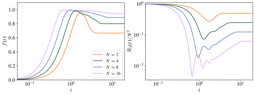
Figure 3: Left: Channel amplitude $f(t)$ (31) for Hilbert-space dimensions $N=2^{k}$ for $k=1,2,3,4$, which captures the strength of the $\operatorname*{tr}(A)\mathds{1}/N$ term in the average channel (30). Right: The two-point SFF $\mathcal{R}_{2}(t)$ (32) normalized by its $t=0$ value of $N^{2}$, for the same values of $N=2^{k}$.

Here we present the average channel $\operatorname{avg}(A,t)=\varphi^{(1)}_{\mathcal{E}}(A,t)$ (22) for a generic ensemble $\mathcal{E}$ that is invariant under rotations in $\mathsf{R}=\mathsf{U}(N)$, such as the GUE [38, 43, 42, 41, 39, 40]. A more detailed derivation appears in App. B.2. In particular, we have that

$$\operatorname{avg}(A,t) =\txintop\nolimits\mathrm{d}\boldsymbol{\lambdaup}\,\rho(\boldsymbol{\lambdaup})\,\sum\limits_{m,n=1}^{N}\,\mathrm{e}^{\mathrm{i}t(\lambdaup_{m}-\lambdaup_{n})}\;\times$$

$$~{}~{}~{}\txintop\nolimits_{\mathsf{R}}\mathrm{d}V\,p(V)\,\,V\lvert m\rangle\langle m\rvert V^{\dagger}\,A\,V\,\lvert n\rangle\langle n\rvert V^{\dagger}\,,~{}$$ (27)

where we omit the “$G$” subscript from $V_{G}$ (B.75) for convenience of presentation. Integrating $V$ and $V^{\dagger}$ over $\mathsf{R}=\mathsf{U}(N)$ with Haar measure leads to [53, 60],

$$\operatorname{avg}(A,t) =\txintop\nolimits\mathrm{d}\boldsymbol{\lambdaup}\,\rho(\boldsymbol{\lambdaup})\sum_{m,n=1}^{N}\,\mathrm{e}^{\mathrm{i}t(\lambdaup_{m}-\lambdaup_{n})}\,\Phi_{mn}(A)\,,~{}$$ (28)

where the operator content is captured by

$$\Phi_{mn}(A) =\frac{N-\delta_{mn}}{N(N^{2}-1)}A+\frac{(N\,\delta_{mn}-1)\,\operatorname*{tr}(A)}{N(N^{2}-1)}\mathds{1}\,,~{}~{}$$ (29)

as we derive explicitly in App. B.2. Integrating over the eigenvalues $\boldsymbol{\lambdaup}$, the average channel (28) becomes

$$\operatorname{avg}(A,t)=[1-f(t)]\,A+\frac{1}{N}\,f(t)\,\operatorname*{tr}(A)\,\mathds{1}\,,~{}~{}$$ (30)

which takes the form of a depolarizing channel [3]. The time-dependent depolarizing parameter is given by

$$f(t)\coloneq\frac{N^{2}-\mathcal{R}_{2}(t)}{N^{2}-1}\,,~{}~{}$$ (31)

which agrees with the results for qubits (9) when $N=2$, and where $\mathcal{R}_{2}(t)$ is the two-point SFF [44, 45, 47, 34, 35, 36, 46] for $\mathcal{E}$, i.e.,

$$\mathcal{R}_{2}(t)\coloneq\mathbb{E}_{\mathcal{E}}\,\sum\limits_{m,n=1}^{N}\,\mathrm{e}^{\mathrm{i}(\lambdaup_{m}-\lambdaup_{n})t}\,,$$ (32)

where $\lambdaup_{m,n}$ are the eigenvalues of the Hamiltonian $G$ (B.74), so that $\mathcal{R}_{2}(t)$ (32) is the Fourier transform of the pair density function of energy eigenvalues of $G$. We calculate this quantity explicitly for the GUE in Sec. 4.1 for any finite $N$. We also note that, because $f(t)$ (31) is an even function, both the Heisenberg evolution of operators $A$ and the Schrödinger evolution of density matrices $\rho$ are described by $\operatorname{avg}(A,t)$ (30), and one need only replace $A\to\rho$ in the latter case.

In Fig. 3, we plot both $f(t)$ (31) and the SFF $\mathcal{R}_{2}(t)$ (32) for the GUE for several values of $N=2^{k}$ (i.e., corresponding to a system of $k$ qubits). Of particular interest is the fact that both $f(t)$ (31) and $\mathcal{R}_{2}(t)$ (32) are nonmonotonic and even functions of $t$. We observe that $f(t)$ vanishes only at $t=0$, never saturates the Haar-random limit $f(t)=1$ (see also Fig. 1), and asymptotes to $f(t)=N/(N+1)$ for $t\gtrsim N$. This can be attributed to properties of the SFF (32), which has value $N^{2}$ at $t=0$, plummets exponentially during an initial “dip” regime, followed by oscillations until the start of a hallmark linear “ramp” regime with $\mathcal{R}_{2}(t)\sim\lvert t\rvert$, before reaching the “plateau” regime with $\mathcal{R}_{2}(t)=N$ for all times $t\geq N$ [44, 45, 47, 34, 35, 36, 46]. We note that the ramp is a signature of chaotic level repulsion, the start of the ramp is known as the “Thouless time,” and the start of the plateau as the “Heisenberg time” [44, 45, 47, 34, 35, 36, 46].

3.3 Variance of the noisy channel

The average channel (30) is the quantity most relevant to experiments on noisy quantum devices. However, it is valuable to diagnose the extent to which that average $\operatorname{avg}(A,t)$ (30) reflects a typical instance $A_{G}(t)$ (18) of noisy unitary evolution. To do so, it is valuable to compare the variance of the channel (23) with the mean (22). As in Sec. 2, we make this comparison at the level of matrix elements $A_{mn}(t)$, and, for convenience, we draw the observable $A$ from the GUE with variance $\sigma_{A}^{2}$.

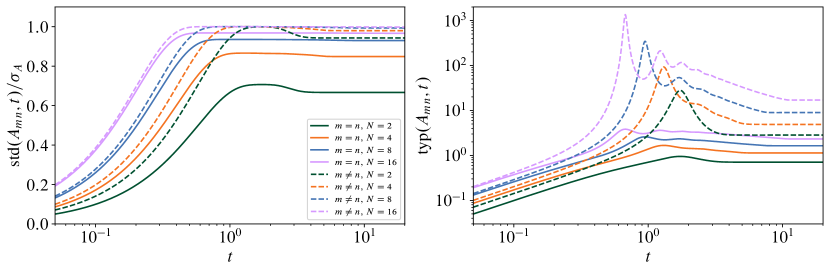
Figure 4: Left: Standard deviation of matrix elements $A_{mn}(t)$ of $A_{G}(t)$ (18), for an initial operator $A$ sampled from the GUE with width $\sigma_{A}$. The standard deviation is the square root of the variance (37), and is plotted in units of $\sigma_{A}$ for various $N=2^{k}$; solid lines denote diagonal elements ($m=n)$ and dashed lines denote off-diagonal elements ($m\neq n$). Right: Plot of the typicality (16) of diagonal (solid) and off-diagonal (dashed) matrix elements $A_{mn}(t)$. The typicality is the standard deviation divided by the square root of (38).

To compute any such variance, we must first calculate the twofold GUE channel (3.1), a special case of the quantity

$$\varphi^{(2)}_{\mathcal{E}}(A,B;t)\coloneq\operatorname{\mathbb{E}}_{\mathcal{E}}\left[A_{G}(t)\otimes B_{G}(t)\right]\,,~{}~{}$$ (33)

which acts on two copies of $\mathcal{H}=\mathbb{C}^{N}$. We note that any operator on $\mathcal{H}^{\otimes 2}$ can be expressed as a linear combination of “basis” operators that factorize over the two copies of $\mathcal{H}$ [36].

The full expression for the twofold channel (33)—even in the case $B=A$ relevant to variances—is too unwieldy for the present discussion, and instead appears in App. B.3, along with a detailed derivation. As with the derivation of the onefold channel (30) in App. B.2, we first average the unitaries $V$ (B.75) over the Haar measure [53, 60], which involves the fourfold Haar channel and its 576 terms. In the case where $B=A$, these terms can be simplified into twelve distinct operators on $\mathcal{H}^{\otimes 2}$ with time-dependent coefficients,

$$\varphi^{(2)}_{\mathcal{E}}\left(A,t\right) =\operatorname{\mathbb{E}}_{\mathcal{E}}\left[\left(\mathrm{e}^{\mathrm{i}Gt}\hskip 0.56905ptA\hskip 0.56905pt\mathrm{e}^{-\mathrm{i}Gt}\right)^{\otimes 2}\right]=\sum\limits_{i=1}^{12}c_{i}(t)\,\mathcal{O}_{i}\,,~{}~{}$$ (34)

which holds for any random-matrix ensemble $\mathcal{E}$ that is invariant under rotations in $\mathsf{R}=\mathsf{U}(N)$, as described in Sec. 3.1.

The operators $\mathcal{O}_{i}$ are given by $\mathds{1}^{\otimes 2}$, $A^{\otimes 2}$, $\operatorname*{tr}(A)\mathds{1}\otimes A$, $\operatorname*{tr}(A)A\otimes\mathds{1}$, $\mathds{1}\otimes A^{2}$, $A^{2}\otimes\mathds{1}$, along with the foregoing six operators multiplied from the right by the SWAP operator $\mathcal{S}$ on $\mathcal{H}^{\otimes 2}$, which for any $\lvert a\rangle,\lvert b\rangle\in\mathcal{H}$ acts as $\mathcal{S}\lvert a\rangle\otimes\lvert b\rangle=\lvert b\rangle\otimes\lvert a\rangle$. This structure is ensured by the Haar averages over $V$ (B.75) alone.

The time-dependent coefficients $c_{i}(t)$, on the other hand, are determined by the spectral PDF $\rho(\boldsymbol{\lambdaup})$ (25). These coefficients depend on combinatoric factors determined by Haar averaging, the two-point SFF $\mathcal{R}_{2}(t)$ (32), as well as two higher-point SFFs [41, 45]. Most straightforward is the four-point SFF,

$$\mathcal{R}_{4}(t)=\operatorname{\mathbb{E}}_{\mathcal{E}}\sum_{k,\ell,m,n}\mathrm{e}^{\mathrm{i}(\lambdaup_{k}+\lambdaup_{\ell}-\lambdaup_{m}-\lambdaup_{n})t}\,,~{}~{}$$ (35)

which is the Fourier transform of the four-point eigenvalue density function. Also relevant to the twofold channel (34) is a three-point SFF, corresponding to

$$\mathcal{R}_{4,1}(t)=\operatorname{\mathbb{E}}_{\mathcal{E}}\sum_{\ell,m,n}\mathrm{e}^{\mathrm{i}(\lambdaup_{\ell}+\lambdaup_{m}-2\lambdaup_{n})t}\,,~{}~{}$$ (36)

where $\mathcal{R}_{4,1}(t)$ denotes the inclusion of one nontrivial Kronecker delta in the summand that defines the four-point SFF $\mathcal{R}_{4}(t)$ (35) [45]. We explicitly evaluate both the higher-point SFFs $\mathcal{R}_{4}(t)$ and $\mathcal{R}_{4,1}(t)$ for the GUE in Sec. 4.3. The full expression for the generic twofold channel (33) in terms of various SFFs and operators on $\mathcal{H}^{\otimes 2}$ (B.92) appears in App. B.3, though it is not particularly enlightening to behold.

To recover a more straightforward diagnostic of the variance of the average channel (30)—and thereby, its typicality—we now consider the variance of individual matrix elements of $A_{G}(t)$ (18), following the treatment of qubits (13) in Sec. 2.

However, we note that the variance of matrix elements depends explicitly on the initial observable $A$; to avoid bias and to simplify presentation, we sample $A$ itself from the GUE with variance $\sigma_{A}^{2}$, in which case we find that

$$\langle\operatorname{var}(A_{mn},t)\rangle^{\vphantom{*}}_{A}=\sigma_{A}^{2}\left(1-\frac{\delta_{m,n}}{N}\right)f(t)\left[2-f(t)\right]\,,~{}~{}$$ (37)

where each factor above is positive semidefinite.

We plot the standard deviation of matrix elements of $A_{G}(t)$ (18) in the left panel of Fig. 4, for several values of $N=2^{k}$. For convenience, we sample $A$ from the $N\times N$ GUE with variance $\sigma_{A}^{2}$. As in Fig. 2, we plot the standard deviation of both diagonal elements (solid) and off-diagonal elements (dashed) of $A_{G}(t)$ (18). We note that the standard deviation is identically zero only at $t=0$, generically nonomonotonic in $t$, and always less than $\sigma_{A}$. We also plot the “typicality” diagnostic (16) in the right panel of Fig. 4 for several values of $N=2^{k}$. The typicality is given by the standard deviation divided by the square root of

$$\langle\operatorname{avg}(A_{mn},t)^{2}\rangle^{\vphantom{*}}_{A} =\sigma_{A}^{2}\left[\left[1-f(t)\right]^{2}+\frac{\delta_{m,n}}{N}f(t)\right]\,,$$ (38)

which follows from the definition of the typicality (16). The result is depicted in the right panel of Fig. 4. Importantly, Fig. 4 reveals that the average (30) is representative of a typical instance of a noisy unitary (18) for the weak-noise regime $t\ll 1$. We also observe that diagonal elements of $A_{G}(t)$ (18) appear to be more typical than off-diagonal elements.

3.4 Higher cumulants

Although we do not evaluate them explicitly herein, one can also use the same RMT methods we use to calculate the average and variance of the noisy channel (18) to compute higher cumulants. The $k$th cumulant extends, e.g., $\operatorname{var}(A,t)$ (33) to $k>2$, and involves the generalized $k$-fold channel (3.1)

$$\varphi^{(k)}_{\mathcal{E}}(A_{1},\dots,A_{k};t)=\operatorname{\mathbb{E}}_{\mathcal{E}}\,\left[\,\bigotimes\limits_{i=1}^{k}\mathrm{e}^{\mathrm{i}Gt}\hskip 0.56905ptA_{i}\hskip 0.56905pt\mathrm{e}^{-\mathrm{i}Gt}\right]\,,~{}$$ (39)

along with various $p$-fold channels for $p<k$.

The evaluation of these $k$-fold GUE channels proceeds in analogy to the discussions in Secs. 3.2 and 3.3. The first step is to perform the Haar average over the diagonalizing unitaries $V$ (B.75). The $k$-fold GUE channel involves the $2k$-fold Haar average (B.89), as described in App. B.3. This average results in $(2k)!^{2}$ terms, corresponding to $(2k)!/k!$ distinct operators on on $\mathcal{H}^{\otimes k}$. As described in App. B.3, the Haar averaging contracts the indices of the various operators $A_{i}$ in (39) multiplied by various Weingarten functions [64, 60, 61, 53] and, separately, contractions of factors $\mathrm{e}^{\pm\mathrm{i}t\lambdaup_{n}}$ (B.74). Each term is multiplied by up to $2k$ factors of the quantity

$$Z(t)\coloneq\operatorname*{tr}(\mathrm{e}^{-\mathrm{i}Gt})=\sum_{m=1}^{N}\mathrm{e}^{-\mathrm{i}t\lambdaup_{m}}\,,~{}$$ (40)

which contribute to the $2k$-point SFF $\mathcal{R}_{2k}(t)$, along with various lower-point SFFs—e.g., $\mathcal{R}_{2}(t)$ (32) and $\mathcal{R}_{4,1}(t)$ (36) both appear in the twofold ($k=2$) channel (23). These lower-point SFFs result from the pairing of eigenvalues due to the Kronecker deltas imposed by the Haar average over the unitaries $V_{G}$ that diagonalize $G$. All of these SFFs are even functions of $t$, and depend on $\rho(\boldsymbol{\lambdaup})$ alone (and not the rotation group $\mathsf{R})$. The structure of operators and coefficients that appear in the $k$-fold GUE channel (3.1) inherit entirely from the fact that $\mathsf{R}=\mathsf{U}(N)$ and that $p(V_{G})$ is the Haar measure on $\mathsf{U}(N)$.

Owing to the unwieldy number of terms that appear in the $k$-fold GUE channel (3.1), it is best to evaluate such higher-fold channels using software capable of symbolic manipulation. To facilitate such calculations, we have supplied a Mathematica notebook containing functions for deriving all operators present in the $k$-fold GUE channel (39) and their time-dependent coefficients. The notebook also details the conversion of these time-dependent coefficients—which involve powers of $Z(t)$ (40)—into generalized SFFs $\mathcal{R}_{2p,\boldsymbol{q}}(t)$ involving $p$ copies of both $Z(t)$ (40) and its conjugate. The $k$-fold GUE channel (3.1) generally involves the SFFs $\mathcal{R}_{2p,\boldsymbol{q}}(t)$ for $p\leq k$, where $\boldsymbol{q}$ encodes which of the $2p$ eigenvalues involved are constrained to be the same (due to Haar averaging $V_{G}$). We evaluate these SFFs for the particular case of the GUE appear in Sec. 4; further details of $k$-fold channels appear in App. B.3.

4 Spectral form factors

One of the fingerprints of quantum chaos—the quantum dynamics that lead to ergodicity and equilibration—is level repulsion in the spectrum of the evolution operator $U(t)=\mathrm{e}^{-\mathrm{i}Gt}$ [41, 45, 50, 44, 46, 34, 35, 36, 47]. This repulsion is an artifact of the spectral rigidity of generic chaotic systems [50, 47, 44, 41, 45, 46, 51]. The simplest probe of spectral rigidity is afforded by the “$r$ ratio” [65]: the average ratio between successive level spacings of $G$. A more detailed probe of spectral statistics is afforded by, e.g., the two-point SFF $\mathcal{R}_{2}(t)$ (32), which is the Fourier transform of the two-point eigenvalue density (or correlation) function of $G$. In particular, the SFF’s linear ramp regime—corresponding to $\mathcal{R}_{2}(t)\sim t$ for $t>\tau_{\text{th}}$, the “Thouless time”—signals the onset of thermalization. Higher moments of eigenvalue distribution of $G$ are probed via higher-point SFFs $\mathcal{R}_{2k}(t)$, along with more general SFFs. In fact, SFFs for Gaussian Hamiltonians $G$ also appear in the context of black holes [46, 41], as well as the various moments of the noisy channel $A_{G}(t)$ (18) discussed in Sec. 3.

In addition to their role in evaluating higher moments of $A_{G}(t)$ (18), the various $p$-point SFFs for Gaussian Hamiltonians $G$ are also interesting in their own right. Here, we provide exact analytic expressions for these SFFs with respect to the GUE with arbitrary $N$. In particular, we evaluate the standard two-point SFF $\mathcal{R}_{2}(t)$ (32) in Sec. 4.1, the three- and four-point SFFs $\mathcal{R}_{4,1}(t)$ (36) and $\mathcal{R}_{4}(t)$ (35), respectively, in Sec. 4.3, and discuss the generalization to higher-point SFFs in Sec. 4.4.

4.1 Two-point SFF

We first consider the standard, two-point SFF $\mathcal{R}_{2}(t)$ (32) that appears in the average GUE channel $\operatorname{avg}(A,t)$ (30),

$$\mathcal{R}_{2}(t) \coloneq\operatorname{\mathbb{E}}_{\text{GUE}}\sum_{m,n=1}^{N}\mathrm{e}^{\mathrm{i}(\lambdaup_{m}-\lambdaup_{n})t}$$

$$\;=N+\operatorname{\mathbb{E}}_{\text{GUE}}\sum_{m\neq n}\mathrm{e}^{\mathrm{i}(\lambdaup_{m}-\lambdaup_{n})t}\,,~{}~{}$$ (41)

where we separate out the diagonal piece for convenience, and the average is taken with respect to $\rho(\boldsymbol{\lambdaup})$ (25). Writing the integral over the spectrum of $G\in\text{GUE}$ explicitly, we define

$$\kappa_{2}(t) \coloneq\frac{1}{N(N-1)}\operatorname{\mathbb{E}}_{\text{GUE}}\sum_{m\neq n}\mathrm{e}^{\mathrm{i}t(\lambdaup_{m}-\lambdaup_{n})}$$

$$\;=\txintop\nolimits\mathrm{d}\lambdaup_{1}\mathrm{d}\lambdaup_{2}\,\rho^{(2)}(\lambdaup_{1},\lambdaup_{2})\ \mathrm{e}^{\mathrm{i}(\lambdaup_{1}-\lambdaup_{2})t}\,,~{}$$ (42)

where $\rho^{(2)}(\lambdaup_{1},\lambdaup_{2})$ is the two-point eigenvalue density function—i.e., the marginal distribution of two eigenvalues, which recovers from integrating $\rho(\boldsymbol{\lambdaup})$ (25) over $N-2$ of its arguments. The integral (42) vanishes after the Heisenberg time $\tau_{\text{Heis}}=N$, consistent with the Riemann-Lebesgue lemma and the expected behavior of the SFF [45, 50, 44, 46, 34, 35, 36, 47].

The two-point eigenvalue density function can be written

$$\rho^{(2)}(\lambdaup_{1},\lambdaup_{2}) =\txintop\nolimits\mathrm{d}\lambdaup_{3}\cdots\mathrm{d}\lambdaup_{N}\,\rho(\boldsymbol{\lambdaup})=\frac{\det_{i,j=1,2}K_{N}(\lambdaup_{i},\lambdaup_{j})}{N(N-1)}\,,~{}$$ (43)

where we used Dyson’s theorem [38] in the second line, and have implicitly defined the GUE kernel,

$$K_{N}(\lambdaup_{i},\lambdaup_{j})\coloneq\sum\limits_{n=0}^{N-1}\phi_{n}(\lambdaup_{i})\phi_{n}(\lambdaup_{j})\,,~{}~{}$$ (44)

in terms of the harmonic-oscillator eigenfunctions

$$\phi_{n}(x)=\left\langle x\middle|n\right\rangle\coloneq(\sqrt{\pi}2^{n}n!)^{-1/2}\mathrm{e}^{-x^{2}/2}H_{n}(x)\,,~{}$$ (45)

where $H_{n}(x)$ is the $n$th (physicist’s) Hermite polynomial. The functions $\phi_{n}(x)$ are the (normalized) eigenfunctions of the harmonic-oscillator Hamiltonian $H=(p^{2}+x^{2})/2$, with corresponding eigenvalues $E_{n}=n+1/2$. Details of these conventions—as well as a brief review of orthonormal polynomial methods in RMT—appear in App. C.

For convenience, we next rewrite $\kappa_{2}(t)$ (42) as

$$\kappa_{2}(t)=\frac{\mathcal{R}_{2,d}(t)+\mathcal{R}_{2,c}(t)}{N(N-1)}\,,~{}~{}$$ (46)

where the subscripts $c$ and $d$ refer to the connected and disconnected contributions, respectively. Defining the “diagonal” harmonic-oscillator integrals

$$\mathcal{I}(t)\coloneq\txintop\nolimits\mathrm{d}\lambdaup\;\mathrm{e}^{-\mathrm{i}t\lambdaup}\,K_{N}(\lambdaup,\lambdaup)=\sum_{n=0}^{N-1}\left\langle*\middle|n\middle|\mathrm{e}^{-\mathrm{i}tx}\right\rangle{n}\,,~{}$$ (47)

along with the “off-diagonal” integrals

$$X_{mn}(t)\coloneq\txintop\nolimits\mathrm{d}\lambdaup\,\mathrm{e}^{-\mathrm{i}t\lambdaup}\phi_{m}(\lambdaup)\phi_{n}(\lambdaup)=\left\langle*\middle|m\middle|\mathrm{e}^{-\mathrm{i}tx}\right\rangle{n}\,,~{}$$ (48)

We can express the disconnected term

$$\mathcal{R}_{2,d}(t)=\mathcal{I}(t)\mathcal{I}(-t)=\left|\sum_{m=0}^{N-1}\left\langle*\middle|m\middle|\mathrm{e}^{-\mathrm{i}tx}\right\rangle{m}\right|^{2}\,,$$ (49)

and for the connected term,

$$\mathcal{R}_{2,c}(t)= -\sum\limits_{m,n=0}^{N-1}X_{mn}(t)X_{nm}(-t)$$

$$= -\sum_{m,n=0}^{N-1}\left\langle*\middle|m\middle|\mathrm{e}^{\mathrm{i}tx}\right\rangle{n}\left\langle*\middle|n\middle|\mathrm{e}^{-\mathrm{i}tx}\right\rangle{m}\,,$$ (50)

in terms of which we rewrite the SFF (32) as

$$\mathcal{R}_{2}(t) =N+\mathcal{R}_{2,d}(t)+\mathcal{R}_{2,c}(t)\,.$$ (51)

The final ingredient required to evaluate the SFF (51) is the form of the matrix elements $\left\langle*\middle|m\middle|\mathrm{e}^{\pm\mathrm{i}tx}\right\rangle{n}$, which can be expressed in terms of generalized Laguerre polynomials [66, 52] as

$$\left\langle*\middle|m\middle|\mathrm{e}^{\alpha x}\right\rangle{n}=\mathrm{e}^{\frac{\alpha^{2}}{4}}\begin{cases}\sqrt{\frac{n!}{m!}}\left(\frac{\alpha}{\sqrt{2}}\right)^{m-n}L_{n}^{m-n}\left(-\frac{\alpha^{2}}{2}\right)&m\geq n\\ \sqrt{\frac{m!}{n!}}\left(\frac{\alpha}{\sqrt{2}}\right)^{n-m}L_{m}^{n-m}\left(-\frac{\alpha^{2}}{2}\right)&m\leq n\end{cases}\,,$$ (52)

so that the SFF (32) can be written as

$$\hskip 2.84526pt\mathcal{R}_{2}(t)=N+\mathrm{e}^{-\frac{t^{2}}{2}}\Big{[}L_{N-1}^{1}\left(\frac{t^{2}}{2}\right)^{2}\\ -\sum_{m,n=0}^{N-1}(-1)^{m-n}L_{n}^{m-n}\left(\frac{t^{2}}{2}\right)L_{m}^{n-m}\left(\frac{t^{2}}{2}\right)\Big{]}\;,~{}$$ (53)

which can be efficiently evaluated for any finite dimension $N$. Further details appear in App. C, and we plot the SFF $\mathcal{R}_{2}(t)$ (53) for various values of $N$ in Fig. 3.

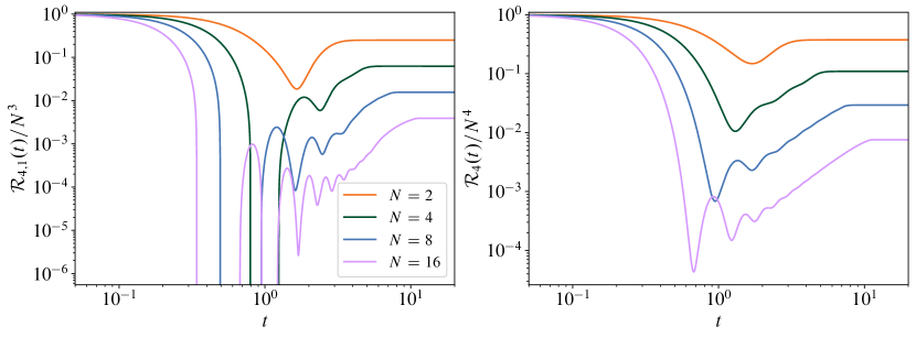
Figure 5: Left: The three-point SFF $\mathcal{R}_{4,1}(t)$ (36) normalized by its $t=0$ value of $N^{3}$, for $N=2^{k}$ with $k=1,2,3,4$. Right: The four-point SFF $\mathcal{R}_{4}(t)$ (35) normalized by its $t=0$ value of $N^{4}$, for the same values of $N=2^{k}$. Both functions bear similarities to $\mathcal{R}_{2}(t)$ (32) [see Fig. 3].

4.2 Three-point SFF

We now consider the three–point SFF (36), given by

$$\mathcal{R}_{4,1}(t)=\operatorname{\mathbb{E}}_{\text{GUE}}\sum_{i,j,k=1}^{N}\mathrm{e}^{\mathrm{i}(\lambdaup_{i}+\lambdaup_{j}-2\lambdaup_{k})t}\,,~{}~{}$$ (54)

which involves the three-point eigenvalue density function

$$\rho^{(3)}(\lambdaup_{1},\lambdaup_{2},\lambdaup_{3})=\frac{(N-3)!}{N!}\det_{i,j=1,2,3}K_{N}(\lambdaup_{i},\lambdaup_{j})\,,$$ (55)

in terms of which we write

$$\mathcal{R}_{4,1}(t)=\txintop\nolimits\mathrm{d}\boldsymbol{\lambdaup}\,\rho(\boldsymbol{\lambdaup})\,\Big{[}N+2\sum\limits_{i\neq j}\mathrm{e}^{\mathrm{i}(\lambdaup_{i}-\lambdaup_{j})t}$$

$$~{}~{}~{}~{}~{}~{}~{}~{}+\sum\limits_{j\neq k}\mathrm{e}^{2\mathrm{i}(\lambdaup_{i}-\lambdaup_{j})t}+\sum\limits_{i\neq j\neq k}\mathrm{e}^{\mathrm{i}(\lambdaup_{i}+\lambdaup_{j}-2\lambdaup_{k})t}\Big{]}\,.~{}$$ (56)

where the indices $i$, $j$, and $k$ are all distinct in the final term. This expression can be further simplified to

$$\mathcal{R}_{4,1}(t) =N+2N(N-1)\kappa_{2}(t)+N(N-1)\kappa_{2}(2t)$$

$$~{}~{}~{}+N(N-1)(N-2)\kappa_{4,1}(t)\,,~{}$$ (57)

where $\kappa_{2}(t)$ is the same function that appears in the two-point SFF $\mathcal{R}_{2}(t)$ (42), and we have implicitly defined the quantity

$$\kappa_{4,1}(t)\coloneq\txintop\nolimits\mathrm{d}\lambdaup_{1}\mathrm{d}\lambdaup_{2}\mathrm{d}\lambdaup_{3}\,\rho^{(3)}(\lambdaup_{1},\lambdaup_{2},\lambdaup_{3})\,\mathrm{e}^{\mathrm{i}\left(\lambdaup_{1}+\lambdaup_{2}-2\lambdaup_{3}\right)t}\,,~{}$$ (58)

which we now investigate further. Using the GUE Kernel (43) and the oscillator eigenfunctions $\phi_{n}(x)$ (45), we have

$$\kappa_{4,1}(t)=\frac{(N-3)!}{N!}\Big{[}\mathcal{I}(t)^{2}\mathcal{I}(2t)+2X_{mn}(t)X_{n\ell}(t)X_{\ell m}(-2t)$$

$$-(2\mathcal{I}(t)X_{mn}(t)X_{nm}(-2t)+\mathcal{I}(2t)X_{mn}(t)X_{nm}(t))\Big{]}\,,~{}~{}$$ (59)

with implicit sums on repeated indices. We do not write the full expression for $\mathcal{R}_{4,1}(t)$ (36) in terms of Laguerre polynomials (facilitated through (52)), as it is quite cumbersome and not nearly as useful to behold as the plot of $\mathcal{R}_{4,1}(t)$ (36) that appears in the left panel of Fig. 5 for several values of $N=2^{k}$. We remark that the three-point SFF (36) has similar properties to the two-point SFF (32) in Fig. 3; however, $\mathcal{R}_{4,1}(t)$ (36) may be negative in the dip regime for $N>2$.

4.3 Four-point SFF

Next we consider the four-point SFF (35), given by

$$\mathcal{R}_{4}(t)=\operatorname{\mathbb{E}}_{\mathcal{E}}\sum_{i,j,k,\ell=1}^{N}\mathrm{e}^{\mathrm{i}(\lambdaup_{i}+\lambdaup_{j}-\lambdaup_{k}-\lambdaup_{\ell})t}\,,~{}~{}$$ (60)

which involves the four-point eigenvalue density function

$$\rho^{(4)}(\lambdaup_{1},\lambdaup_{2},\lambdaup_{3},\lambdaup_{4})=\frac{(N-4)!}{N!}\det_{i,j=1,2,3,4}K_{N}(\lambdaup_{i},\lambdaup_{j})\,.$$ (61)

As before (57), we separate the various terms corresponding to distinct sums over eigenvalues, finding

$$\mathcal{R}_{4}(t) =N(2N-1)+4N(N-1)^{2}\kappa_{2}(t)+\frac{N!}{(N-2)!}\kappa_{2}(2t)$$

$$~{}~{}+2\frac{N!}{(N-3)!}\kappa_{4,1}(t)+\frac{N!}{(N-4)!}\kappa_{4}(t)\,,~{}$$ (62)

which involves $\kappa_{2}(t)$ (42), $\kappa_{4,1}(t)$ (4.2), and the new quantity

$$\kappa_{4}(t)\coloneq\txintop\nolimits\mathrm{d}\vec{\lambdaup}\,\rho^{(4)}(\vec{\lambdaup})\,\mathrm{e}^{\mathrm{i}\left(\lambdaup_{1}+\lambdaup_{2}-\lambdaup_{3}-\lambdaup_{4}\right)t}\,,~{}$$ (63)

where we used the shorthand $\vec{\lambdaup}=\{\lambdaup_{1},\lambdaup_{2},\lambdaup_{3},\lambdaup_{4}\}$ for notational convenience. As before, we evaluate $\kappa_{4}(t)$ (63) using a determinant of the Gaussian kernel $K_{N}(\lambdaup_{i},\lambdaup_{j})$ (44), but now with four distinct eigenvalues. We find that

$$\kappa_{4}(t)= \frac{(N-4)!}{N!}[\mathcal{I}^{4}-2\mathcal{I}^{2}X^{\vphantom{*}}_{mn}X^{\vphantom{*}}_{nm}-4\mathcal{I}^{2}X^{\vphantom{*}}_{mn}X_{nm}^{*}$$

$$~{}~{}~{}~{}+8\mathcal{I}X^{\vphantom{*}}_{mn}X^{\vphantom{*}}_{n\ell}X_{\ell m}^{*}+2X_{mn}^{2}X_{nm}^{*2}+X_{mn}^{2}X_{nm}^{2}$$

$$~{}~{}~{}~{}-4X^{\vphantom{*}}_{mn}X^{\vphantom{*}}_{n\ell}X_{\ell k}^{*}X_{km}^{*}-2X^{\vphantom{*}}_{mn}X_{n\ell}^{*}X^{\vphantom{*}}_{\ell k}X_{km}^{*}]\,,~{}~{}$$ (64)

in terms of the harmonic-oscillator integrals $\mathcal{I}(t)$ (47) and $X_{mn}(t)$ (48), whose time dependence we have suppressed for compactness. Numerical evaluation is again facilitated using (52), in terms of generalized Laguerre polynomials. Using the above expression for $\kappa_{4}(t)$ (64), as well as previously derived expressions for $\kappa_{4,1}(t)$ and $\kappa_{2}(t)$, we recover an exact analytic expression for the four-point SFF $\mathcal{R}_{4}(t)$ (62) for any finite $N$. In turn, this furnishes an exact analytic expression of the variance (23) of the GUE channel (18), which agrees with the single-qubit result (13) when $N=2$.

However, the full expression for $\mathcal{R}_{4}(t)$ (60) is again quite cumbersome and we do not write it explicitly; instead, a plot of $\mathcal{R}_{4}(t)$ appears in Fig. 5 for several values of $N=2^{k}$. Its phenomenology mirrors that of the two-point SFF (32) in Fig. 3.

4.4 Higher-point SFFs

The methods used to compute the SFFs $\mathcal{R}_{2}(t)$ (53), $\mathcal{R}_{4,1}(t)$ (36), and $\mathcal{R}_{4}(t)$ (60) also extend to arbitrary SFFs of the form $\mathcal{R}_{2p,\boldsymbol{q}}(t)$. The first step is to write $\mathcal{R}_{2p,\boldsymbol{q}}(t)$ as a sum over unique sets of nonrepeating eigenvalues, as for the two-point (41) and three-point (56) SFFs. This also ameliorates any potential issues that could arise when $2p-q>N$ (so that eigenvalues must be repeated), as with the evaluation of the single-qubit variance channel (11). See also App. B.3.

The result of this expansion is a sum over various functions $\kappa_{2p^{\prime},\boldsymbol{q^{\prime}}}(t)$, as with the two-point (42), three-point (57), and four-point (62) SFFs. Each function $\kappa_{2p^{\prime},\boldsymbol{q^{\prime}}}(t)$ involves an integral over a complex exponential of $k=2p^{\prime}-q^{\prime}$ nonrepeating eigenvalues and the $k$-point eigenvalue density function $\rho^{(k)}(\lambdaup_{1},\dots,\lambdaup_{k})$. By Dyson’s theorem [38], we have that

$$\rho^{(k)}(\lambdaup_{1},\ldots,\lambdaup_{k})=\frac{(N-k)!}{N!}\det_{i,j=1,\ldots,k}K_{N}(\lambdaup_{i},\lambdaup_{j})\,,~{}$$ (65)

where the kernel $K_{N}(\lambdaup_{i},\lambdaup_{j})$ (44) has a simple expression in terms of normalized harmonic-oscillator eigenfunctions (45).

Hence, $\mathcal{R}_{2p,\boldsymbol{q}}(t)$ can be written as a sum of functions $\kappa_{2p^{\prime},\boldsymbol{q^{\prime}}}(t)$ multiplied by $N$-dependent coefficients. The functions $\kappa_{2p^{\prime},\boldsymbol{q^{\prime}}}(t)$ are integrals over $\boldsymbol{\lambdaup}=\{\lambdaup_{1},\dots,\lambdaup_{2p^{\prime}-q^{\prime}}\}$ of various factors $\smash{\mathrm{e}^{\pm\mathrm{i}t\lambdaup_{n}}}$ times $\smash{\rho^{(k)}(\boldsymbol{\lambdaup})}$ (65) for $k=2p^{\prime}-q^{\prime}$. Owing to the structure of the kernel $K_{N}(\lambdaup_{i},\lambdaup_{j})$ (44), each eigenvalue $\lambdaup_{n}$ appears in an expression of the form

$$\txintop\nolimits\mathrm{d}\lambdaup\,\mathrm{e}^{\pm\mathrm{i}t\lambdaup}\phi_{m}(\lambdaup)\phi_{n}(\lambdaup)\mathrm{e}^{-\lambdaup^{2}}=\left\langle*\middle|m\middle|\mathrm{e}^{\pm\mathrm{i}tx}\right\rangle{n}\,,~{}$$ (66)

which is simply a matrix element of the complex exponential of the position operator $x$ in the harmonic-oscillator language, which contributes to integral expressions of the form $\mathcal{I}(t)$ (47) or $X_{mn}(t)$ (48). These functions—and the matrix elements (66) themselves—can be written in terms of a sum over finitely many generalized Laguerre polynomials (52) [66, 52], leading to an exact analytic expression for any $\mathcal{R}_{2p,\boldsymbol{q}}(t)$ eigenvalues.

5 Outlook

We have developed an exact analytic toolbox for describing noisy quantum evolution that can be smoothly tuned to the identity map. The noise is captured by unitary evolution under a Hamiltonian $G$ drawn from an RMT ensemble that is invariant under rotations $G\to VGV^{\dagger}$ for $V$ belonging to some group $\mathsf{R}$ (e.g., $\mathsf{R}=\mathsf{U}(N)$ for the GUE). This guarantees that integrals over $G$ simplify greatly to integrals over the spectrum of $G$ and over $\mathsf{R}$ with Haar measure. The latter integrals are often known, and the former lead to spectral form factors, which are relevant to quantum chaos [50, 44, 46, 45, 41, 47, 34, 35, 36, 51, 49, 52]. The channels may act on the physical system of interest, a subset thereof, and/or on ancilla degrees of freedom representing the environment; various symmetries and constraints may be imposed via projectors (see Refs. 34, 35, 36 for details).

We compute the average of noisy evolutions $\mathrm{e}^{\mathrm{i}Gt}\hskip 0.56905ptA\hskip 0.56905pt\mathrm{e}^{-\mathrm{i}Gt}$ (18) with respect to $G$ exactly. The result $\operatorname{avg}(A,t)$ takes the form of a time-dependent depolarization channel (30) [3]. Importantly, the time-dependent amplitudes (i) depend on the noise strength $\sigma$ and duration $t$ only through the product $\sigma t$, (ii) depend on $t$ only through the two-point SFF $\mathcal{R}_{2}(\sigma t)$ (32), (iii) are nonmonotonic functions of $\sigma t$, and (iv) never saturate the Haar-random limit $\operatorname{avg}(A,t)\propto\mathds{1}$ (see Fig. 3). We also compute the variance of matrix elements of $\mathrm{e}^{\mathrm{i}Gt}\hskip 0.56905ptA\hskip 0.56905pt\mathrm{e}^{-\mathrm{i}Gt}$ (18), which we use to diagnose typicality (16). We observe that the average channel $\operatorname{avg}(A,t)$ (30) reflects a typical instance of noisy evolution $\mathrm{e}^{\mathrm{i}Gt}\hskip 0.56905ptA\hskip 0.56905pt\mathrm{e}^{-\mathrm{i}Gt}$ (18)—in the sense that $\operatorname{typ}(A_{mn},t)\ll 1$—in the weak-noise limit $\sigma t\lesssim 1$. We also sketch the evaluation of higher cumulants to diagnose the noisy evolution in detail, and have included a Mathematica notebook for doing so [67].

The foregoing calculations apply to noisy evolution generated by any ensemble invariant under $\mathsf{R}=\mathsf{U}(N)$, and depend only on the corresponding SFF $\mathcal{R}_{2}(t)$ (32) for the spectral distribution. We compute the SFFs $\mathcal{R}_{2}(t)$ (32), $\mathcal{R}_{4,1}(t)$ (36), and $\mathcal{R}_{4}(t)$ (35) for the GUE exactly for any finite $N$ for the first time in terms of generalized Laguerre polynomials (see Fig. 5). Our results for $\mathcal{R}_{2}(t)$ (32) correct typos that appear in Ref. 49. We also sketch how to evaluate the higher-point SFFs relevant to higher cumulants of the noisy channel, which we also expect to be of interest to the study of quantum chaos and even black holes.

Although we primarily restricted to the GUE for simplicity, the methods we outline extend to other rotation-invariant random-matrix ensembles $\mathcal{E}$. Importantly, we expect that averaging over noisy evolutions results in more interesting effective channels for ensembles beyond the GUE, as is the case for the Gaussian orthogonal (GOE) and symplectic (GSE) ensembles [56], whose averages do not have the form of a depolarizing channel. Our methods are also compatible with the three standard Wishart-Laguerre ensembles [57, 43], and the various Altland-Zirnbauer ensembles [58]. In general, the choice of ensemble should be dictated by experimental considerations and symmetry properties. We also note that additional structure (e.g., symmetries and/or constraints) can be enforced on the noisy unitaries using appropriate projectors [34, 35, 36]. We expect the application of this method to other ensembles—and to the diagnosis of quantum phases of matter and the robustness to noise of various protocols for tomography—to be of great utility to various areas of quantum science.

There are several promising applications for our methodology and directions for future work. In the context of condensed matter, our methods allow one to establish the existence of (possibly nonequilibrium) quantum phases of matter by probing the robustness of the universal properties to noise. In the context of atomic, molecular, and optical physics, it is relevant to identifying whether the dominant sources of noise are coherent or incoherent, and to make quantitative predictions for time evolutions subject to coherent noise. Our framework is also extremely relevant to QEC in various contexts [4, 5, 6, 7, 8, 9, 10, 11, 12, 13]: Our exact results for qubits (without averaging) can be used to test the efficacy of error-correction protocols by modeling all noise as (possibly correlated) single-qubit unitary errors; our results for general $N$ may also be useful to probing the efficacy of error-correction protocols. Furthermore and most importantly, our framework may be used to improve randomized benchmarking [68, 69, 70, 71, 72, 73] either by (i) incorporating block structure to diagnose noise that respects a particular symmetry or obeys a particular constraint or (ii) drawing $G$ from an ensemble other than the GUE, resulting in a channel that is not in the depolarizing form, yielding more detailed information than Haar-random benchmarking (or any 2-design). Finally, our methods may be used to diagnose the sensitivity to noise between shots of various protocols that require multiple copies of a quantum state $\rho$, including cross-entropy diagnostics and all forms of state and process tomography [19, 20, 21].

Data availability.—The Mathematica notebook used to perform Haar averaging is available on Zenodo [67].

Appendix A Gaussian unitary ensemble

For the sake of clarity, we explicitly define the Gaussian unitary ensemble GUE$(N,\sigma)$ of complex $N\times N$ Hermitian matrices [38], and discuss various properties of this random-matrix ensemble. We provide two equivalent definitions:

1. The ensemble GUE$(N,\sigma)$ consists of all $N\times N$ matrices $G$ whose diagonal elements $G_{ii}\in\mathbb{R}$ are drawn from the (real) normal distribution $\mathcal{N}_{\mathbb{R}}(0,\sigma^{2})$ and whose upper-triangular elements $G_{ij}\in\mathbb{C}$ for $i<j$ are drawn from the (complex) normal distribution $\mathcal{N}_{\mathbb{C}}(0,\sigma^{2})$. The lower-triangular elements are defined as $G_{ij}\coloneq G^{*}_{ji}$ for $i>j$.

2. The ensemble GUE$(N,\sigma)$ consists of all $N\times N$ matrices $G$ of the form $G\coloneq(X+X^{\dagger})/2$, where all components of the matrix $X$ are independently drawn from the (complex) normal distribution $\mathcal{N}_{\mathbb{C}}(0,\sigma^{2}/2)$.

Note that the complex normal distribution satisfies $\mathcal{N}_{\mathbb{C}}(0,\sigma)\sim\mathcal{N}_{\mathbb{R}}(0,\sigma^{2}/2)+\mathrm{i}\,\mathcal{N}_{\mathbb{R}}(0,\sigma^{2}/2)$; i.e., the real and complex parts are independently drawn from a normal distribution with half the variance. As a result, all elements $G_{ij}$ of the Gaussian matrix $G\in\text{GUE}(N,\sigma)$ have variance $\sigma^{2}$.

Using straightforward algebraic manipulations, the product of the probability density functions (PDFs) for the individual matrix elements of a Gaussian unitary matrix $G\in\text{GUE}(N,\sigma)$ can be rewritten as the following PDF for $G$ itself,

$$P_{\text{GUE}}(G,\sigma)=\frac{1}{Z}\exp\left[-\frac{1}{2\sigma^{2}}\operatorname*{tr}(G^{2})\right]\,,~{}~{}$$ (A.67)

subject to the constraint that $G=G^{\dagger}$ is Hermitian, where the “partition function” $Z$ ensures normalization of $P$ (A.67). The corresponding one-point eigenvalue density function $\rho_{1}(\lambdaup)$ realizes Wigner’s semicircle law [38],

$$\rho_{1}(\lambdaup)=\frac{1}{2\pi\sigma^{2}N}\sqrt{4N\sigma^{2}-\lambdaup^{2}}+\cdots,$$ (A.68)

to leading order as $N\to\infty$; the “$\cdots$” term above reflects subleading corrections, which vanish faster than $N^{-1/2}$.

For convenience, we take $\sigma=1/\sqrt{2}$ throughout the main text, in which case the PDF for a complex, Hermitian matrix $G$ sampled from the GUE takes the form

$$P_{\text{GUE}}(G)=\frac{1}{\Omega}\exp\left[-\operatorname*{tr}(G^{2})\right]\,,$$ (A.69)

and the “strength” of the noisy unitary $U_{G}=\mathrm{e}^{-\mathrm{i}tG}$ is controlled simply by the time $t$. This choice is particularly convenient for the computation of the spectral form factor (related to the average channel) for arbitrary $N$ in Sec. 4, because the physicists’ Hermite polynomials form a basis with respect to the Gaussian measure (A.69). For this choice of $\sigma=2^{-1/2}$, the corresponding semicircle law (A.68) takes the familiar form

$$\rho_{1}(\lambdaup)=\frac{1}{\pi N}\sqrt{2N-\lambdaup^{2}}\,,~{}~{}$$ (A.70)

up to corrections that vanish as $1/N$ or faster.

Appendix B Ensemble averaging

Here we provide explicit details of the ensemble-averaging procedure summarized in Sec. 3. We define rotational invariance in App. B.1, showing that the eigenvectors of Gaussian unitaries are Haar random and other details relevant to Sec. 3.1. In App. B.2, we utilize known results for Haar integrals to obtain the exact form of the average noisy channel (30) that is the main result of this work and Sec. 3.2. In App. B.3, we use similar methods to derive the twofold channel (34), which we use to diagnose typicality of the average channel in Sec. 3.3.

B.1 Rotation Invariance

A powerful constraint on RMT ensembles derives from rotation invariance, which we now elucidate. An RMT ensemble $\mathcal{E}$ corresponds to a PDF $P_{\mathcal{E}}(G)$ over matrices $G$ belonging to a subspace $\mathcal{E}$ of the space $M_{N}(\mathbb{C})$ of complex $N\times N$ matrices. The subspace $\mathcal{E}$ is generally specified by defining how the components $G_{ij}$ of $G$ are sampled (see for example the construction of elements $G$ of the GUE in App. A).

An random-matrix ensemble $\mathcal{E}$ with PDF $P_{\mathcal{E}}(G)$ is invariant under a rotation group $\mathsf{R}$ if the following conditions hold:

1. For any $G_{0}\in\mathcal{E}$ and for all $Q\in\mathsf{R}$, we have that

   $$G^{\prime}=Q\hskip 0.56905ptG_{0}\hskip 0.56905ptQ^{\dagger}\in\mathcal{E}\,.~{}$$ (B.71)

2. For any $G_{0}\in\mathcal{E}$ and $Q\in\mathsf{R}$, we have that

   $$P_{\mathcal{E}}(G^{\prime})=P_{\mathcal{E}}(Q\hskip 0.56905ptG_{0}\hskip 0.56905ptQ^{\dagger})=P_{\mathcal{E}}(G)\,.~{}$$ (B.72)

3. For any $G_{0}\in\mathcal{E}$, the rotation matrix $V^{\smash{\vphantom{\dagger}}}_{\smash{G}}$ that diagonalizes $G_{0}$ is itself an element of $\mathsf{R}$, i.e.,

   $$V_{\smash{G}}^{\smash{\dagger}}\hskip 0.56905ptG_{0}\hskip 0.56905ptV_{\smash{G}}^{\smash{\vphantom{\dagger}}}=\operatorname{diag}(\boldsymbol{\lambdaup})~{}\implies~{}V^{\smash{\vphantom{\dagger}}}_{\smash{G}}\in\mathsf{R}\,.~{}~{}$$ (B.73)

The first condition ensures that conjugating elements of $\mathcal{E}$ by elements of $\mathsf{R}$ returns an element of $\mathcal{E}$. The second condition is the standard meaning of rotation invariance of $P_{\mathcal{E}}(G)$. The third condition is essential to simplifying ensemble averages; note that the physically relevant choices of $\mathcal{E}$ are ensembles of Hermitian matrices of exponentials thereof, which are always diagonalizable. It is sufficient for the above if (i) the diagonalized version of every element of $\mathcal{E}$ is also an element of $\mathcal{E}$ and (ii) the image of the adjoint action of $\mathsf{R}$ on $\mathcal{E}$ is precisely $\mathcal{E}$. We also comment that, in the presence of block structure [34, 35, 36], the conditions above hold within each block individually.

Before using rotation invariance to simplify averages over the RMT ensemble $\mathcal{E}$, we first rewrite the PDF $P_{\mathcal{E}}(G)$ in terms of the spectral decomposition of $G\in\mathcal{E}$,

$$P_{\mathcal{E}}(G)\,\mathrm{d}G=\rho(\boldsymbol{\lambdaup})\,p(V^{\vphantom{\dagger}}_{\smash{G}})\hskip 0.56905pt\mathrm{d}\boldsymbol{\lambdaup}\hskip 0.56905pt\mathrm{d}V^{\vphantom{\dagger}}_{\smash{G}}\,,~{}~{}$$

where $\boldsymbol{\lambdaup}=\{\lambdaup_{1},\lambdaup_{2},\dots,\lambdaup_{N}\}$ contains the $N$ eigenvalues of $G$, $\rho(\boldsymbol{\lambdaup})$ is the joint PDF of the $N$ eigenvalues of $G$, and $p(V^{\smash{\vphantom{\dagger}}}_{\smash{G}})$ is the PDF for the unitary matrix $V^{\smash{\vphantom{\dagger}}}_{\smash{G}}$ that diagonalizes $G$, and whose columns are normalized eigenvectors of $G$.

As a sanity check for the validity of (25), we may check that both sides of (25) contain the same number of degrees of freedom. We begin by writing $G$ in the form

$$G=\sum\limits_{n=1}^{N}\lambdaup_{n}\,\lvert\psi_{n}\rangle\langle\psi_{n}\rvert=\sum\limits_{n=1}^{N}\lambdaup_{n}\,V^{\vphantom{\dagger}}_{\smash{G}}\,\lvert n\rangle\langle n\rvert V^{\dagger}_{\smash{G}}\,.$$ (B.74)

Additionally, the $n$th column of $V^{\smash{\,}}_{\smash{G}}$ gives the components of the eigenvector $\lvert\psi_{n}\rangle$ in the $\{\lvert n\rangle\}$ basis, i.e.,

$$\left\langle*\middle|m\middle|V_{\smash{G}}\right\rangle{n}=\left\langle m\middle|\psi_{n}\right\rangle~{}\implies~{}V_{\smash{G}}=\sum\limits_{n=1}^{N}\,\lvert\psi_{n}\rangle\langle n\rvert\,,~{}$$ (B.75)

so that $G_{\text{diag}}=V^{\dagger}_{\smash{G}}\hskip 1.13809ptG\hskip 1.13809ptV^{\vphantom{\dagger}}_{\smash{G}}$ is diagonal in the $\{\lvert n\rangle\}$ basis. Importantly, $G_{\text{diag}}$ commutes with any diagonal unitary $U_{\text{diag}}=\operatorname{diag}(\mathrm{e}^{\mathrm{i}\theta_{1}},\dots,\mathrm{e}^{\mathrm{i}\theta_{N}})$—equivalently, each ket $\lvert\psi_{n}\rangle$ in the outer-product definition of $V^{\,}_{\smash{G}}$ (B.75) is only unique up to a complex phase $\mathrm{e}^{\mathrm{i}\theta_{n}}$. Consequently, the diagonalizing unitary $V^{\,}_{\smash{G}}$ (B.75) is only uniquely defined up to some $U_{\text{diag}}$. Hence, the diagonalizing unitary $V^{\,}_{\smash{G}}$ (B.75) is specified by $\smash{N^{2}-N}$ real, compact parameters, compared to $\smash{N^{2}}$ for an arbitrary element of $\mathsf{U}(N)$. Combined with the $N$ eigenvalues $\{\lambdaup_{n}\}$ leads to $\smash{N^{2}}$ real parameters, as needed to specify an element of the GUE [38, 43, 42].

The change of variables (25) is useful because all conjugation-invariant functions of a matrix $G$—e.g., the probability distribution $P_{\mathcal{E}}(G)$—can be expressed in terms of traces of powers of $G$, which can be expressed entirely in terms of the eigenvalues of $G$ (since the determinant is related to the traces via the Cayley-Hamilton Theorem). For Gaussian ensembles, e.g., only $\smash{\operatorname*{tr}(G^{2})}$ and $\operatorname*{tr}(G)$ are needed [74]. As derived in, e.g., Ref. 38, for the GUE with PDF $P_{\mathcal{E}}(G)$ (A.67), we have that

$$\rho(\boldsymbol{\lambdaup})=\frac{1}{\Omega}\mathrm{e}^{-\boldsymbol{\lambdaup}^{2}/2\sigma^{2}}\,\lvert\Delta(\boldsymbol{\lambdaup})\rvert^{2}\,,~{}~{}$$ (B.76)

where $\boldsymbol{\lambdaup}^{2}=\lambdaup_{1}^{2}+\cdots+\lambdaup_{N}^{2}$ and the object $\Delta(\boldsymbol{\lambdaup})$ is simply the Vandermonde determinant, given by

$$\Delta(\boldsymbol{\lambdaup})\coloneq\prod\limits_{i<j}(\lambdaup_{i}-\lambdaup_{j})\,,~{}~{}$$ (B.77)

which comes from the change of variables captured by (25). Other choices of ensembles $\mathcal{E}$ will result in different joint eigenvalue density functions $\rho(\boldsymbol{\lambdaup})$ above.

We now invoke rotation invariance of $\mathcal{E}$, and specifically, of $P_{\mathcal{E}}(G)$ (B.72). The requirement that the diagonalizing matrix $V_{G}$ is an element of $\mathsf{R}$ (B.73) immediately implies that

$$P_{\mathcal{E}}(G)=P_{\mathcal{E}}(V_{\smash{G}}^{\smash{\dagger}}\hskip 0.56905ptG\hskip 0.56905ptV^{\smash{\vphantom{\dagger}}}_{\smash{G}})=P_{\mathcal{E}}(D)\,,~{}~{}$$ (B.78)

where $D=V_{\smash{G}}^{\smash{\dagger}}\hskip 0.56905ptG\hskip 0.56905ptV^{\smash{\vphantom{\dagger}}}_{\smash{G}}=\operatorname{diag}(\boldsymbol{\lambdaup})$ is the diagonalized version of $G\in\mathcal{E}$, so schematically, $P_{\mathcal{E}}(D)\sim\rho(\boldsymbol{\lambdaup})$. Importantly, since $\mathsf{R}$ is a group, rotation invariance of $P_{\mathcal{E}}(G)$ (B.72) also implies that

$$P_{\mathcal{E}}(G)=P_{\mathcal{E}}(W^{\dagger}V_{\smash{G}}^{\smash{\dagger}}U^{\dagger}\hskip 0.56905ptG\hskip 0.56905ptUV^{\smash{\vphantom{\dagger}}}_{\smash{G}}W)=P_{\mathcal{E}}(D)\,,~{}~{}$$ (B.79)

for any $U,W\in\mathsf{R}$. Combining the foregoing relation with the spectral decomposition (25), we conclude that

$$p(U\hskip 0.56905ptV^{\smash{\vphantom{\dagger}}}_{\smash{G}}\hskip 0.56905ptW)=p(V^{\smash{\vphantom{\dagger}}}_{\smash{G}})~{}~{}\forall\,U,W\in\mathsf{R}\,,~{}~{}$$ (B.80)

which is known as left-right invariance of $p(V^{\smash{\vphantom{\dagger}}}_{\smash{G}})$ over $\mathsf{R}$. This is ensured by the requirement that $V^{\smash{\vphantom{\dagger}}}_{\smash{G}}\in\mathsf{R}$ (B.73). Importantly, the only measure $p(V^{\smash{\vphantom{\dagger}}}_{\smash{G}})$ satisfying left-right invariance (B.80) for a compact matrix group $\mathsf{R}$ is the Haar measure, which is uniform over $\mathsf{R}$ [59, 60, 61, 62, 63]. This is a useful result because averages over the Haar measure $p(V^{\smash{\vphantom{\dagger}}}_{\smash{G}})$ are generally the most straightforward of all RMT ensembles, and have been worked out for the compact matrix groups $\mathsf{R}$ of interest [53, 41, 59, 60, 61, 62, 63, 75, 76].

B.2 Onefold average

The most important quantity we compute is the onefold channel (22), associated with the average over noisy unitary evolutions (18) generated by GUE Hamiltonians; here, we provide a detailed derivation of the result (30). To start, it is useful to write the noisy unitary in the form

$$U_{G}(t) \coloneq\mathrm{e}^{-\mathrm{i}Gt}=\sum_{m=1}^{N}\mathrm{e}^{-\mathrm{i}\lambdaup_{m}t}\,V^{\smash{\vphantom{\dagger}}}_{\smash{G}}\lvert m\rangle\langle m\rvert V^{\smash{\dagger}}_{\smash{G}}$$

$$=\sum_{i,j,m=1}^{N}\mathrm{e}^{-\mathrm{i}\lambdaup_{m}t}V^{\smash{\vphantom{*}}}_{im}V^{\smash{*}}_{mj}\,\lvert i\rangle\langle j\rvert\,,~{}~{}$$ (B.81)

in the computational basis in which the components of $G$ are drawn, where $V$ diagonalizes $G$ (B.73), so that the $m$th column of $V$ is a normalized eigenvector of $G$ with eigenvalue $\lambdaup_{m}$—i.e., $V_{im}=\left\langle i\middle|\psi_{m}\right\rangle$, where $G\lvert\psi_{m}\rangle=\lambdaup_{m}\lvert\psi_{m}\rangle$.

We then consider the Heisenberg evolution of an observable $A$ under $U_{G}(t)$ (B.81), captured by the adjoint action

$$A(t)=U_{\smash{G}}^{\smash{\dagger}}\hskip 0.56905ptA\hskip 0.56905ptU_{\smash{G}}^{\smash{\vphantom{\dagger}}}=\mathrm{e}^{\mathrm{i}Gt}\hskip 0.56905ptA\hskip 0.56905pt\mathrm{e}^{-\mathrm{i}Gt}\,,~{}~{}$$

where the evolution of a density matrix $\rho$ under $U_{G}(t)$ (B.81) is captured by taking $A\to\rho$ and $t\to-t$ above. Expanding $A(t)$ (18) in the computational basis, we have

$$A(t) =\sum\limits_{i,j,m,n,\mu,\nu}\mathrm{e}^{\mathrm{i}(\lambdaup_{m}-\lambdaup_{n})t}V^{\smash{\vphantom{*}}}_{\mu m}V^{\smash{*}}_{mi}A^{\smash{\vphantom{*}}}_{\smash{i}j}V^{\smash{\vphantom{*}}}_{jn}V^{\smash{*}}_{n\nu}\lvert\mu\rangle\langle\nu\rvert\,,~{}$$ (B.82)

which we then simplify by averaging $V$ with respect to $p(V)$ (B.80). Owing to rotation invariance, as discussed in App. B.1, averaging $V$ over $\mathsf{U}(N)$ is straightforward, because $p(V)$ is simply the (uniform) Haar measure.

The average over $V$ in $A(t)$ (B.82) corresponds to the twofold Haar average over $\mathsf{U}(N)$ [53, 59, 60, 61, 62, 63], i.e.,

$$~{}\txintop\nolimits\mathrm{d}\mu(V)\,V^{\smash{\vphantom{*}}}_{\smash{a}_{1}b_{1}}V^{\smash{\vphantom{*}}}_{\smash{a}_{2}b_{2}}V^{\smash{*}}_{\smash{a}_{3}b_{3}}V^{\smash{*}}_{\smash{a}_{4}b_{4}}=\frac{1}{N^{2}-1}\times$$

$$\left[\delta^{a_{1}b_{1}a_{2}b_{2}}_{a_{3}b_{3}a_{4}b_{4}}+\delta^{a_{1}b_{1}a_{2}b_{2}}_{a_{4}b_{4}a_{3}b_{3}}-\frac{1}{N}\left(\delta^{a_{1}b_{1}a_{2}b_{2}}_{a_{3}b_{4}a_{4}b_{3}}+\delta^{a_{1}b_{1}a_{2}b_{2}}_{a_{4}b_{3}a_{3}b_{4}}\right)\right],$$ (B.83)

where, for convenience, we have used the shorthand

$$\delta^{\,ab\dots}_{\alpha\beta\dots}=\delta_{a,\alpha}\delta_{b,\beta}\cdots\,,~{}~{}$$ (B.84)

and applying the result (B.83) to $A(t)$ (B.82) leads to

$$\txintop\nolimits\mathrm{d}\mu(V)\,A(t)=\sum_{\begin{subarray}{c}i,j,m\\ n,\mu,\nu\end{subarray}}\mathrm{e}^{\mathrm{i}(\lambdaup_{m}-\lambdaup_{n})t}\frac{1}{N^{2}-1}A^{\smash{\vphantom{*}}}_{\smash{i}j}\lvert\mu\rangle\langle\nu\rvert\,\times$$

$$\left[\delta_{\mu,i}\delta_{j,\nu}+\delta_{\mu,\nu}\delta_{m,n}\delta_{i,j}-\frac{1}{N}\left(\delta_{\mu,i}\delta_{m,n}\delta_{j,\nu}+\delta_{\mu,\nu}\delta_{i,j}\right)\right]\,,$$

and summing over $i$ and $j$ leads to

$$\txintop\nolimits\mathrm{d}\mu(V)\,A(t)=\sum_{m,n,\mu,\nu}\frac{\mathrm{e}^{\mathrm{i}(\lambdaup_{m}-\lambdaup_{n})t}}{N^{2}-1}\lvert\mu\rangle\langle\nu\rvert\times$$

$$\left[\left(1-\frac{\delta_{m,n}}{N}\right)A_{\mu,\nu}+\operatorname*{tr}(A)\left(\delta_{m,n}-\frac{1}{N}\right)\delta_{\mu,\nu}\right]\,,~{}$$

and, finally, summing over $\mu$ and $\nu$ gives

$$=\sum\limits_{m,n=0}^{N-1}\frac{\mathrm{e}^{\mathrm{i}(\lambdaup_{m}-\lambdaup_{n})t}}{N^{2}-1}\left[\left(1-\frac{\delta_{m,n}}{N}\right)A+\operatorname*{tr}(A)\left(\delta_{m,n}-\frac{1}{N}\right)\mathds{1}\right]\,,~{}$$

and for further simplification, we recall the definition

$$Z(t)\coloneq\operatorname*{tr}(\mathrm{e}^{-\mathrm{i}Gt})=\sum_{m=1}^{N}\mathrm{e}^{-\mathrm{i}t\lambdaup_{m}}\,,$$

in terms of which we can write

$$\sum_{m,n=1}^{N}\mathrm{e}^{\mathrm{i}(\lambdaup_{m}-\lambdaup_{n})t}\left(1-\frac{\delta_{m,n}}{N}\right) =\lvert Z(t)\rvert^{2}-1$$ (B.85a)

$$\sum_{m,n=1}^{N}\mathrm{e}^{\mathrm{i}(\lambdaup_{m}-\lambdaup_{n})t}\left(\delta_{m,n}-\frac{1}{N}\right) =N-\lvert Z(t)\rvert^{2}\,,~{}~{}$$ (B.85b)

so that we can write the Haar average of $A(t)$ (B.82) as

$$\txintop\nolimits\mathrm{d}\mu(V)A(t)=\frac{\lvert Z(t)\rvert^{2}-1}{N^{2}-1}A+\frac{N^{2}-\lvert Z(t)\rvert^{2}}{N^{2}-1}\frac{\operatorname*{tr}(A)}{N}\mathds{1}\,,$$ (B.86)

and noting that the quantity

$$\mathcal{R}_{2}(t)=\txintop\nolimits_{\mathcal{E}}\mathrm{d}\boldsymbol{\lambdaup}\,\rho(\boldsymbol{\lambdaup})\lvert Z(t)\rvert^{2}\,,~{}~{}$$ (B.87)

is the two-point SFF (32) [41, 44, 45, 47, 34, 35, 36, 46], averaging (B.86) over the eigenvalues $\boldsymbol{\lambdaup}$ with respect to $\rho(\boldsymbol{\lambdaup})$ (25) leads to

$$\varphi^{(1)}_{\mathcal{E}}(A,t)=\frac{\mathcal{R}_{2}(t)-1}{N^{2}-1}A+\frac{N^{2}-\mathcal{R}_{2}(t)}{N^{2}-1}\frac{\operatorname*{tr}(A)}{N}\mathds{1}\,,$$ (B.88)

which recovers the result (30) of the main text upon identifying $f(t)$ (31) in terms of the SFF (B.87). Note that this particular form (B.88) holds for any random-matrix ensemble that is invariant under rotations in $\mathsf{R}=\mathsf{U}(N)$, as described in App. B.1, where $\mathcal{R}_{2}(t)$ (B.87) is determined by $\rho(\boldsymbol{\lambdaup})$ (25) alone.

B.3 Twofold and higher averages

Diagnosing the typicality of the average channel (30) involves calculating the variance of matrix elements of $A(t)$ (B.82). That, in turn, requires the evaluation of the twofold GUE channel, whose most general form is given by

$$\varphi^{(2)}_{\mathcal{E}}(A,B;t) \coloneq\operatorname{\mathbb{E}}_{\mathcal{E}}\left[\left(\mathrm{e}^{\mathrm{i}Gt}A\mathrm{e}^{-\mathrm{i}Gt}\right)\otimes\left(\mathrm{e}^{\mathrm{i}Gt}B\mathrm{e}^{-\mathrm{i}Gt}\right)\right]$$

$$\;=\txintop\nolimits\mathrm{d}G\,P_{\mathcal{E}}(G)\,A_{G}(t)\otimes B_{G}(t)\,,~{}$$ (33)

which acts on $\mathcal{H}^{\otimes 2}=\mathbb{C}^{N}\otimes\mathbb{C}^{N}$. Note that generic operators on $\mathcal{H}^{\otimes 2}$ may be decomposed onto a basis of operators [36] that factorize over the two copies of $\mathcal{H}$. The case relevant to calculating variances corresponds to $B=A$; we evaluate the general version with $B\neq A$ in the interest of thoroughness.

We perform the average over $G$ using the same strategy as in App. B.2 for the onefold channel (22). First, we write the time-evolved operators $A_{G}(t)$ and $B_{G}(t)$ (18) in terms of the eigenvalues $\boldsymbol{\lambdaup}$ and eigenvectors $V$ of $G$ (B.82). We then integrate over the diagonalizing unitaries, corresponding to the fourfold Haar average over $\mathsf{U}(N)$. The final step is the average over the eigenvalues of $G$, resulting in SFFs.

Although we are presently concerned with the twofold GUE channel, the procedure we outline applies to generic $k$-fold GUE channels. The first step is to compute the $2k$-fold Haar average over the $V$s. The result involves a sum over $(2k)!^{2}$ permutations, where combinatoric factors called Weingarten functions [64, 60, 61, 53] encode the “weight” of each permutation. Evaluating the $2k$-fold Haar average over $V\in\mathsf{U}(N)$ leads to

$$\txintop\nolimits_{\mathsf{U}(N)}\mathrm{d}\mu(V)\,V^{\smash{\vphantom{\dagger}}}_{\smash{a}_{1}b_{1}}\cdots V^{\smash{\vphantom{\dagger}}}_{\smash{a}_{2k}b_{2k}}\,V^{\smash{*}}_{\smash{\alpha}_{1}\beta_{1}}\cdots V^{\smash{*}}_{\smash{\alpha}_{2k}\beta_{2k}}=\\ \sum_{\pi,\tau\in S_{2k}}\operatorname{Wg}(N,\tau^{-1}\pi)\,\delta_{a_{1}\cdots a_{2k}}^{\pi(\alpha_{1})\cdots\pi(\alpha_{2k})}\delta_{b_{1}\cdots b_{2k}}^{\tau(\beta_{1})\cdots\tau(\beta_{2k})}\,,~{}$$ (B.89)

where $V^{*}$ is the complex conjugate of $V$ (not to be confused with the adjoint $V^{\dagger}$) and $\pi$ and $\tau$ denote independent permutations of $2k$ objects (the group $S_{2k}$), corresponding to all ways of independently pairing the two indices of $V$s with those of $V^{*}$s [53, 60, 41]. Going forward, we omit the explicit dependence on $N$ of the Weingarten function $\operatorname{Wg}$, and refer only to the cycle structure of the contractions of $V$s with $V^{*}$s (B.89). For example, the contraction that pairs each $a_{j}$ and $b_{j}$ with its corresponding $\alpha_{j}$ and $\beta_{j}$, respectively, results in $2k$ cycles of length one—the Weingarten function for this contraction is denoted $\operatorname{Wg}(1^{2k})$. The sum of all cycle lengths is always $2k$.

For $k>1$, the resulting expressions are quite cumbersome and not particularly enlightening (although we compute an exact expression for $k=2$ below, owing to its relation to the variance). Even enumerating the number of operators on $\mathcal{H}^{\otimes k}$ as a function of $k$ is challenging. For this reason, the Haar averages described above essentially must be worked out on a case-by-case basis using any computer algebra system. For the reader interested in such calculations, we have included a Mathematica notebook with functions for enumerating all contractions and assigning the appropriate Weingarten functions.

Because the unitaries $V$ (B.75) are contracted with the operators $A_{m}$ (for $1\leq m\leq k$) and the eigenvalues $\mathrm{e}^{\pm\mathrm{i}t\lambdaup_{n}}$, the Haar average (B.89) results in turn imposes a contraction on the indices of $A_{m}$ and $\mathrm{e}^{\pm\mathrm{i}t\lambdaup_{n}}$. It so happens that the Haar average does not mix between these two sets: the components of $A$ and the overall operator on $\mathcal{H}^{\otimes k}$ may be contracted, and the eigenvalues $\mathrm{e}^{\pm\mathrm{i}t\lambdaup_{n}}$ may also be independently contracted. The former results in various combinations of the $A_{m}$ operators and their traces—along with permutation operators on $\mathcal{H}^{\otimes k}$ that send the state $\lvert a_{1},\dots,a_{k}\rangle$ to some permutation $\lvert\pi(a_{1},\dots,a_{k})\rangle$. For $k=2$, there is only the SWAP operator $\mathcal{S}=\sum_{a,b}\lvert ab\rangle\langle ba\rvert$. The latter contractions result in expressions of the form

$$\sum\limits_{\begin{subarray}{c}m_{1},\dots,m_{k}\\ n_{1},\dots,n_{k}\end{subarray}}\mathrm{e}^{\mathrm{i}t\left(\lambdaup_{m_{1}}+\cdots+\lambdaup_{m_{k}}-\lambdaup_{n_{1}}-\cdots-\lambdaup_{n_{k}}\right)}\,\delta^{\dots}_{\dots}~{},~{}~{}$$ (B.90)

where $\delta^{\dots}_{\dots}$ denotes arbitrary contractions amongst the indices $m_{i}$, $n_{j}$. The result of the contractions is an SFF of the form

$$\mathcal{R}_{2p,\boldsymbol{q}}(t)=\txintop\nolimits\mathrm{d}\boldsymbol{\lambdaup}\,\rho(\boldsymbol{\lambdaup})Z(t)^{p}Z^{*}(t)^{p-q}\prod_{i=1}^{n}Z^{*}(q_{i}t)\,,~{}$$ (B.91)

where again, $1\leq p\leq k$, $\boldsymbol{q}=\{q_{1},\dots,q_{n}\}$, $q=\sum_{i}q_{i}<p$, and $Z^{*}(t)$ is the complex conjugate of $Z(t)$ (40). Essentially, Kronecker deltas between indices $m_{i}$ and $n_{j}$ (B.90) result in $p<k$, while Kronecker deltas between indices $m_{i}$ and $m_{j}$ (or between $n_{i}$ and $n_{j}$) result in $q>0$. When $q=0$, $\mathcal{R}_{2p,0}(t)=\mathcal{R}_{2p}(t)$ is the $2p$-point SFF, the Fourier transform of the $2p$-point eigenvalue density function [45]. When $q=\sum_{i}q_{i}>0$, the result is a $(2p-q)$-point SFF [45]—e.g., $\mathcal{R}_{4,1}(t)$ (36) is a three-point SFF. Note that all SFFs (B.91) are even functions of $t$, meaning that contractions between the $m$ indices or the $n$ indices both result in the same SFF $\mathcal{R}_{2p,\boldsymbol{q}}(t)$ (B.91). We discuss the evaluation of such higher-point SFFs in Sec. 4.4.

However, we comment that some care must be taken in the case $2k>N$ [53, 60, 61, 47, 34]. Naïvely, the generic $2k$-fold Haar average (B.89) is only defined when $2k<N$ (i.e., the number of copies of $V$ and its conjugate are no greater than $N$). However, Ref. 61 proved that the Haar averages computed for $2k<N$ [53, 60] also apply even when $N>2k$. Most importantly, although the Weingarten functions for the $2k$-fold channel (B.93) contain denominators with factors $(N^{2}-j^{2})$ for $0\leq j<2k$, there are never divergences in the final result [61]. The resolution comes from the SFFs that appear in the $k$-fold GUE channel, which generally results in the $2k$-point and lower SFFs (B.91). However, the $p$-point SFF is only defined for $p\leq N$; for $p>N$, it reduces to lower-point SFFs multiplied by polynomial functions of $N$. These additional factors of $N$ that come from identifying valid SFFs for $2k>N$ precisely cancel the singular denominators that appear in the Weingarten functions (B.93). This occurs, e.g., in the case of qubits, which have a well defined variance—corresponding to the fourfold Haar average—despite the presence of factors of $(N^{2}-4)$ in the denominators of the Weingarten functions that appear in the twofold GUE channel (B.93), even though $2k>N$.

We now return to the particular case of $k=2$ and the twofold channel (33). For convenience, we group terms according to their operator content on $\mathcal{H}^{\otimes 2}$, finding that

$$\varphi^{(2)}(A,B;t)=C_{A,B}(t)\,A\otimes B+C_{B,A}(t)\,B\otimes A$$

$$+C_{1,A}(t)\left[\operatorname*{tr}(B)\mathds{1}\otimes A+\operatorname*{tr}(A)B\otimes\mathds{1}+\mathcal{S}\left(\mathds{1}\otimes BA+AB\otimes\mathds{1}\right)\right]$$

$$+C_{A,1}(t)\left[\operatorname*{tr}(B)A\otimes 1+\operatorname*{tr}(A)\mathds{1}\otimes B+\mathcal{S}\left(\mathds{1}\otimes AB+BA\otimes\mathds{1}\right)\right]$$

$$+C_{\operatorname*{tr}(A)\operatorname*{tr}(B)}(t)\left[\operatorname*{tr}(A)\operatorname*{tr}(B)+\operatorname*{tr}(AB)\mathcal{S}\right]\mathds{1}^{\otimes 2}$$

$$+C_{\operatorname*{tr}(AB)}(t)\left[\operatorname*{tr}(AB)+\operatorname*{tr}(A)\operatorname*{tr}(B)\mathcal{S}\right]\mathds{1}^{\otimes 2}$$

$$+C_{1,AB}(t)\left[\mathds{1}\otimes\left(AB+BA\right)+\left(AB+BA\right)\otimes\mathds{1}\right.$$

$$~{}~{}~{}+\left.\operatorname*{tr}(B)\mathcal{S}\left(\mathds{1}\otimes A+A\otimes\mathds{1}\right)+\operatorname*{tr}(A)\mathcal{S}\left(\mathds{1}\otimes B+B\otimes\mathds{1}\right)\right]$$

$$+C_{\mathcal{S}}(t)\,\mathcal{S}\left(A\otimes B+B\otimes A\right)\,,~{}~{}$$ (B.92)

where the coefficients $C(t)$ also depend on $N$, and are given by

$$C_{A,B}(t) =N\operatorname{Wg}(3)-4\operatorname{Wg}(1^{4})\mathcal{R}_{2}(t)+\operatorname{Wg}(2^{2})\mathcal{R}_{2}(2t)+2\operatorname{Wg}(1^{2},2)\mathcal{R}_{4,1}(t)+\operatorname{Wg}(1^{4})\mathcal{R}_{4}(t)$$

$$C_{B,A}(t) =-N\operatorname{Wg}(3)-4\operatorname{Wg}(2^{2})\mathcal{R}_{2}(t)+\operatorname{Wg}(1^{4})\mathcal{R}_{2}(2t)+2\operatorname{Wg}(1^{2},2)\mathcal{R}_{4,1}(t)+\operatorname{Wg}(2^{2})\mathcal{R}_{4}(t)$$

$$C_{1,A}(t) =2\left[\operatorname{Wg}(1^{2},2)+N\operatorname{Wg}(1,3)\right]\mathcal{R}_{2}(t)+\operatorname{Wg}(1^{2},2)\mathcal{R}_{2}(2t)+2\operatorname{Wg}(1,3)\mathcal{R}_{4,1}(t)+\operatorname{Wg}(4)\mathcal{R}_{4}(t)$$

$$C_{A,1}(t) =N\operatorname{Wg}(1,2)+\left[N\operatorname{Wg}(1^{4})-\operatorname{Wg}(1^{2},2)\right]\mathcal{R}_{2}(t)+\operatorname{Wg}(4)\mathcal{R}_{2}(2t)+2\operatorname{Wg}(1,3)\mathcal{R}_{4,1}(t)+\operatorname{Wg}(1^{2},2)\mathcal{R}_{4}(t)$$

$$C_{\operatorname*{tr}(A)\operatorname*{tr}(B)}(t) =N\operatorname{Wg}(1^{3})-2\left[\operatorname{Wg}(1^{4})+\operatorname{Wg}(2^{2})\right]\mathcal{R}_{2}(t)+\operatorname{Wg}(2^{2})\mathcal{R}_{2}(2t)+2\operatorname{Wg}(4)\mathcal{R}_{4,1}(t)+\operatorname{Wg}(2^{2})\mathcal{R}_{4}(t)$$

$$C_{\operatorname*{tr}(AB)}(t) =N\operatorname{Wg}(1,2)-4\operatorname{Wg}(1^{2},2)\mathcal{R}_{2}(t)+\operatorname{Wg}(4)\mathcal{R}_{2}(2t)+2\operatorname{Wg}(2^{2})\mathcal{R}_{4,1}(t)+\operatorname{Wg}(4)\mathcal{R}_{4}(t)$$

$$C_{1,AB}(t) =-\operatorname{Wg}(1,2)-\left[\operatorname{Wg}(1^{4})+3\operatorname{Wg}(1,3)-\operatorname{Wg}(2^{2})\right]\mathcal{R}_{2}(t)+\operatorname{Wg}(1,3)\mathcal{R}_{2}(2t)$$

$$\quad~{}~{}~{}+\left[\operatorname{Wg}(1^{2},2)+\operatorname{Wg}(4)\right]\mathcal{R}_{4,1}(t)+\operatorname{Wg}(1,3)\mathcal{R}_{4}(t)$$

$$C_{\mathcal{S}}(t) =-4\operatorname{Wg}(1^{2},2)\mathcal{R}_{2}(t)+\operatorname{Wg}(1^{2},2)\mathcal{R}_{2}(2t)+\left[\operatorname{Wg}(1^{4})+\operatorname{Wg}(2^{2})\right]\mathcal{R}_{4,1}(t)+\operatorname{Wg}(1^{2},2)\mathcal{R}_{4}(t)\,.~{}~{}$$ (B.93)

Appendix C Spectral form factors for the GUE

Evaluating the $k$-fold GUE channel $\varphi^{(k)}(A,t)$ (3.1) requires an analytic expression for the $2k$-point SFF, as well as lower-point SFFs. These SFFs also have applications to quantum chaos and even black holes [50, 44, 46, 45, 41, 47, 34, 35, 36, 51, 49, 52]. The SFFs depend only on the eigenvalue density function $\rho(\boldsymbol{\lambdaup})$ (25), which for Gaussian ensembles [38, 43, 42, 41, 39, 40] is given by

$$\rho(\boldsymbol{\lambdaup})\equiv\frac{1}{\Omega}\prod_{i<j}\left|\lambdaup_{i}-\lambdaup_{j}\right|^{2}\exp\left(-\frac{\beta}{2}\sum_{i=1}^{N}\lambdaup_{i}^{2}\right)\,,~{}~{}$$

where we take $\beta=2$ for the GUE. The standard tactic for evaluating integrals over eigenvalue distributions is known as the “orthogonal-polynomial method” [38].

C.1 Orthogonal Polynomials

Evaluating the standard, two-point SFF $\mathcal{R}_{2}(t)$ (32) requires integration of $\cos[t(\lambdaup_{1}-\lambdaup_{2})]$ over the GUE eigenvalues $\lambdaup_{1}\neq\lambdaup_{2}$. Higher-point SFFs require similar integrals over nonrepeating eigenvalues $\{\lambdaup_{1},\dots,\lambdaup_{m}\}$; these integrals can be evaluated using the marginal eigenvalue PDF

$$\rho^{(m)}\left(\lambdaup_{1},\dots,\lambdaup_{m}\right)\coloneq\txintop\nolimits\mathrm{d}\lambdaup_{m+1}\dots\mathrm{d}\lambdaup_{N}\,\rho(\boldsymbol{\lambdaup})\,,~{}$$ (C.94)

where $\rho(\boldsymbol{\lambdaup})$ (25) is the full eigenvalue density function. We expect these integrals to be tractable for generic RMT ensembles whose eigenvalue distributions $\rho(\boldsymbol{\lambdaup})$ are known (e.g., due to rotation invariance), such as the GUE (26).

Integrals involving the PDF (26) and its marginals (C.94) are simplified substantially with the use of a complete, orthonormal basis of (polynomial) functions. In particular, the invariance of the Vandermonde determinant $\smash{\Delta(\boldsymbol{\lambdaup})=\prod_{i<j}\left(\lambdaup_{i}-\lambdaup_{j}\right)=\det[\mathcal{V}(\boldsymbol{\lambdaup})]}$ under elementary row operations on the Vandermonde matrix (which satisfies $\mathcal{V}_{ij}=\lambdaup_{i}^{j}$ for $0\leq i,j<N$, with $\lambdaup_{0}=1$) guarantees that $\smash{\lvert\Delta(\boldsymbol{\lambdaup})\rvert^{2}}$ can be conveniently expressed in the form of a finite sum of inner products (44), using any basis set of polynomials. The measure $\smash{\mathrm{e}^{-\lambdaup^{2}}}$ (26) associated with each eigenvalue $\lambdaup$ suggests that a pragmatic choice of basis corresponds to the (physicist’s) Hermite polynomials $\{H_{n}(\lambdaup)\}$, which form a complete orthogonal basis for the Hilbert space $L^{2}(\mathbb{R})$, i.e.,

$$\txintop\nolimits_{\mathbb{R}}\mathrm{d}x\,\mathrm{e}^{-x^{2}}\,H_{m}(x)H_{n}(x)=\pi^{1/2}2^{n}n!\,\delta_{m,n}\,.$$ (C.95)

For convenience, we use harmonic oscillator eigenstates, whose $n$th normalized basis function is given by

$$\phi_{n}(x)=\left\langle x\middle|n\right\rangle=\left(\sqrt{\pi}2^{n}n!\right)^{-1/2}\mathrm{e}^{-x^{2}/2}H_{n}(x)\,.$$ (45)

Crucially, writing the marginal PDF $\smash{\rho^{(m)}(\boldsymbol{\lambdaup})}$ (C.94) in the basis of Hermite polynomials $H_{n}(x)$ (C.95) is particularly convenient. For example, for $m=2$ we have

$$\rho^{(2)}(\lambdaup_{1},\lambdaup_{2}) =\frac{(N-2)!}{N!}\det\begin{pmatrix}K_{N}^{i,i}&K_{N}^{i,j}\\ K_{N}^{j,i}&K_{N}^{j,j}\end{pmatrix},$$ (C.96)

where the kernel function has a simple representation in terms of the basis functions $\phi_{n}$ (45),

$$K_{N}^{i,j}=K_{N}(\lambdaup_{i},\lambdaup_{j})\coloneq\sum\limits_{n=0}^{N-1}\phi_{n}(\lambdaup_{i})\phi_{n}(\lambdaup_{j})\,,~{}~{}$$ (44)

and expressing the $m$-point eigenvalue PDF $\rho^{(m)}(\boldsymbol{\lambdaup})$ (C.94) as a determinant (C.96) of the GUE kernel functions $K_{N}$ (44) leads to a relatively straightforward analytical expression for the SFF. For the two-point SFF (32), e.g., we have

$$\mathcal{R}_{2}(t)=N+N(N-1)\kappa_{2}(t)\,,~{}~{}$$ (C.97)

where we have introduced the function

$$\kappa_{2}(t)\coloneq\txintop\nolimits\mathrm{d}\lambdaup_{1}\mathrm{d}\lambdaup_{2}\,\rho^{(2)}(\lambdaup_{1},\lambdaup_{2})\ \mathrm{e}^{\mathrm{i}(\lambdaup_{1}-\lambdaup_{2})t}\,,~{}$$ (42)

as an integral over $\rho^{(2)}(\lambdaup_{1},\lambdaup_{2})$, which we express in terms of the kernel functions $K_{N}(\lambdaup_{i},\lambdaup_{j})$ (C.96). Using the harmonic-oscillator eigenbasis for $K_{N}(\lambdaup_{i},\lambdaup_{j})$ (44), we arrive at an expression for $\kappa_{2}(t)$ (42) in terms of integrals of the form

$$\txintop\nolimits\mathrm{d}\lambdaup\,\mathrm{e}^{\pm\mathrm{i}\lambdaup t}\,\phi_{m}(\lambdaup)\phi_{n}(\lambdaup)=\left\langle*\middle|m\middle|\mathrm{e}^{\pm\mathrm{i}xt}\right\rangle{n}\,,~{}$$ (C.98)

where $x$ is the position operator for the harmonic oscillator with Hamiltonian $H=(p^{2}+x^{2})/2$, where $\phi_{n}(x)$ (45) is an eigenstate of this Hamiltonian with eigenvalue $n+1/2$. These methods also extend to higher-point SFFs (see Sec. 4).

C.2 Harmonic oscillator matrix elements

Having reduced generic SFFs to harmonic-oscillator matrix elements of the form $\left\langle*\middle|m\middle|\mathrm{e}^{\pm\mathrm{i}tx}\right\rangle{n}$ (C.98), we now derive an explicit analytical form for these quantities in terms of generalized Laguerre polynomials. Similar treatments appear in Refs. 66 and 52; a proof is given below for convenience.

Evaluating such matrix elements is most straightforward in the language of the bosonic raising and lowering operators $a$ and $a^{\dagger}$, respectively, where the lowering operator $a$ acts as

$$a^{k}\lvert m\rangle=\sqrt{\frac{m!}{(m-k)!}}\lvert m-k\rangle\,,~{}~{}$$ (C.99)

for $k,m\in\mathbb{N}$ with $m\geq k$, where $[a,a^{\dagger}]=\mathds{1}$. In terms of this annihilation operator $a$ and its conjugate, the position and momentum operators can be written

$$x=\frac{a+a^{\dagger}}{\sqrt{2}}~{},~{}~{}p=\frac{a-a^{\dagger}}{\mathrm{i}\sqrt{2}}\,,~{}~{}$$ (C.100)

so that $[x,p]=\mathrm{i}\mathds{1}$, as expected. A relevant relation is

$$\mathrm{e}^{\alpha x}=\mathrm{e}^{\alpha(a+a^{\dagger})/\sqrt{2}}=\mathrm{e}^{\alpha^{2}/4}\mathrm{e}^{\alpha a^{\dagger}/\sqrt{2}}\mathrm{e}^{\alpha a/\sqrt{2}}$$ (C.101)

and combining this relation (which follows straightfowardly from a Baker-Campbell-Hausdorff expansion) with the action (C.99) gives for the relevant matrix element (52),

$$\left\langle*\middle|m\middle|\mathrm{e}^{\alpha x}\right\rangle{n} =\left\langle*\middle|m\middle|\mathrm{e}^{\alpha^{2}/4}\mathrm{e}^{\alpha a^{\dagger}/\sqrt{2}}\mathrm{e}^{\alpha a/\sqrt{2}}\right\rangle{n}$$

$$=\mathrm{e}^{\frac{\alpha^{2}}{4}}\sum\limits_{j=0}^{m}\sum\limits_{k=0}^{n}\frac{1}{j!k!}\left(\frac{\alpha^{2}}{2}\right)^{\frac{j+k}{2}}\left\langle*\middle|m\middle|(a^{\dagger})^{j}a^{k}\right\rangle{n}$$

$$=\mathrm{e}^{\frac{\alpha^{2}}{4}}\sum\limits_{j,k=0}^{m,n}\frac{\alpha^{j+k}}{j!k!}\sqrt{\frac{2^{-j-k}\,m!\,n!}{(m-j)!(n-k)!}}\left\langle m-j\middle|n-k\right\rangle\,,$$

and for $$m\geq n$$, we have that

$$=\mathrm{e}^{\frac{\alpha^{2}}{4}}\sum\limits_{k=0}^{n}\frac{\alpha^{2k+m-n}}{(k+m-n)!\,k!}2^{-k}\sqrt{\frac{2^{n-m}\,m!\,n!}{(n-k)!^{2}}}\,,~{}$$

$$=\mathrm{e}^{\frac{\alpha^{2}}{4}}\sum\limits_{k=0}^{n}\frac{\alpha^{2k+m-n}}{(k+m-n)!\,k!}2^{-k}\sqrt{\frac{2^{n-m}\,m!\,n!}{(n-k)!^{2}}}\,,~{}$$

$$=\mathrm{e}^{\frac{\alpha^{2}}{4}}\left(\frac{\alpha}{\sqrt{2}}\right)^{m-n}\sqrt{\frac{n!}{m!}}\sum\limits_{k=0}^{n}\frac{1}{k!}\left(\frac{\alpha^{2}}{2}\right)^{k}\begin{pmatrix}m\\ n-k\end{pmatrix}$$

$$=\mathrm{e}^{\frac{\alpha^{2}}{4}}\sqrt{\frac{n!}{m!}}\left(\frac{\alpha}{\sqrt{2}}\right)^{m-n}L^{m-n}_{n}\left(-\frac{\alpha^{2}}{2}\right)\,,~{}$$ (C.102)

where $L^{m-n}_{n}(x)$ is the generalized Laguerre polynomial; among other relations, these polynomials satisfy the Rodrigues formula

$$L_{n}^{(a)}(x) \coloneq\frac{x^{a}\,\mathrm{e}^{x}}{n!}\frac{\mathrm{d}^{n}}{\mathrm{d}x^{n}}\left(x^{n+a}\mathrm{e}^{-x}\right)$$

$$\;=\frac{x^{-a}}{n!}\left(\frac{\mathrm{d}}{\mathrm{d}x}-1\right)^{n}x^{n+a}\,,~{}$$ (C.103)

for $a\geq 0$; the case $\alpha=0$ realizes the “simple” Laguerre polynomials $L_{n}^{(0)}(x)=L_{n}(x)$, which form a complete set of orthogonal polynomials with respect to the measure $\mathrm{e}^{-x}$.

For the case $m\leq n$, we instead have

$$\left\langle*\middle|m\middle|\mathrm{e}^{\alpha x}\right\rangle{n} =\mathrm{e}^{\frac{\alpha^{2}}{4}}\sqrt{\frac{m!}{n!}}\left(\frac{\alpha}{\sqrt{2}}\right)^{n-m}L^{n-m}_{m}\left(-\frac{\alpha^{2}}{2}\right)\,,~{}$$ (C.104)

i.e., the roles of $m$ and $n$ are swapped compared to the $m\geq n$ case (C.102). One can also derive the $m\leq n$ result (C.104) from the $m\geq n$ result (C.102) using the relation

$$L^{(-a)}_{n}(x)=\frac{(n-a)!}{n!}(-x)^{a}L^{a}_{n+a}(x)\,,~{}~{}$$ (C.105)

for integers $a>0$.

References

- Preskill [2012] J. Preskill, Quantum computing and the entanglement frontier (2012), arXiv:1203.5813 [quant-ph] .
- Preskill [2018] J. Preskill, Quantum 2, 79 (2018).
- Nielsen and Chuang [2010] M. A. Nielsen and I. L. Chuang, Quantum Computation and Quantum Information: 10th Anniversary Edition (Cambridge University Press, 2010).
- Calderbank and Shor [1996] A. R. Calderbank and P. W. Shor, Phys. Rev. A 54, 1098 (1996).
- Steane [1996a] A. Steane, Proc. Roy. Soc. London. A: MPES 452, 2551 (1996a).
- Steane [1996b] A. M. Steane, Phys. Rev. Lett. 77, 793 (1996b).
- DiVincenzo and Shor [1996] D. P. DiVincenzo and P. W. Shor, Phys. Rev. Lett. 77, 3260 (1996).
- Kitaev [1997] A. Y. Kitaev, Rus. Math. Surveys 52, 1191 (1997).
- Gottesman [1998] D. Gottesman, Phys. Rev. A 57, 127 (1998).
- Knill et al. [2000] E. Knill, R. Laflamme, and L. Viola, Phys. Rev. Lett. 84, 2525 (2000).
- Dennis et al. [2002] E. Dennis, A. Kitaev, A. Landahl, and J. Preskill, J. Math. Phys. 43, 4452 (2002).
- Temme et al. [2017] K. Temme, S. Bravyi, and J. M. Gambetta, Phys. Rev. Lett. 119, 180509 (2017).
- Lieu et al. [2020] S. Lieu, R. Belyansky, J. T. Young, R. Lundgren, V. V. Albert, and A. V. Gorshkov, Phys. Rev. Lett. 125, 240405 (2020).
- Cruz et al. [2019] D. Cruz, R. Fournier, F. Gremion, A. Jeannerot, K. Komagata, T. Tosic, J. Thiesbrummel, C. L. Chan, N. Macris, M.-A. Dupertuis, and C. Javerzac-Galy, Adv. Quant. Tech. 2 (2019).
- Satzinger et al. [2021] K. J. Satzinger, Y. Liu, A. Smith, C. Knapp, M. Newman, C. Jones, and et al., Science 374, 1237 (2021).
- Friedman et al. [2023a] A. J. Friedman, C. Yin, Y. Hong, and A. Lucas, Locality and error correction in quantum dynamics with measurement (2023a), arXiv:2206.09929 [quant-ph] .
- Lu et al. [2022] T.-C. Lu, L. A. Lessa, I. H. Kim, and T. H. Hsieh, PRX Quantum 3, 040337 (2022).
- Haah et al. [2021] J. Haah, M. B. Hastings, R. Kothari, and G. H. Low, SIAM J. Sci. Comput. , FOCS18 (2021).
- Huang et al. [2020] H.-Y. Huang, R. Kueng, and J. Preskill, Nature Phys. 16, 1050–1057 (2020).
- Huang et al. [2022a] H.-Y. Huang, M. Broughton, J. Cotler, S. Chen, J. Li, M. Mohseni, H. Neven, R. Babbush, R. Kueng, J. Preskill, and J. R. McClean, Science 376, 1182–1186 (2022a).
- Huang et al. [2022b] H.-Y. Huang, R. Kueng, G. Torlai, V. V. Albert, and J. Preskill, Science 377, eabk3333 (2022b).
- Pezzè et al. [2018] L. Pezzè, A. Smerzi, M. K. Oberthaler, R. Schmied, and P. Treutlein, Rev. Mod. Phys. 90, 035005 (2018).
- Ma et al. [2011] J. Ma, X. Wang, C. Sun, and F. Nori, Phys. Reports 509, 89 (2011).
- Daniel and Miyake [2021] A. K. Daniel and A. Miyake, Phys. Rev. Lett. 126, 090505 (2021).
- Bulchandani et al. [2023a] V. B. Bulchandani, F. J. Burnell, and S. L. Sondhi, Phys. Rev. B 107, 045412 (2023a).
- Bulchandani et al. [2023b] V. B. Bulchandani, F. J. Burnell, and S. L. Sondhi, Phys. Rev. B 107, 035409 (2023b).
- Daniel et al. [2022] A. K. Daniel, Y. Zhu, C. H. Alderete, V. Buchemmavari, A. M. Green, N. H. Nguyen, T. G. Thurtell, A. Zhao, N. M. Linke, and A. Miyake, Phys. Rev. Res. 4, 033068 (2022).
- Hart et al. [2024] O. Hart, D. T. Stephen, D. J. Williamson, M. Foss-Feig, and R. Nandkishore, Playing nonlocal games across a topological phase transition on a quantum computer (2024), arXiv:2403.04829 [quant-ph] .
- Guo et al. [2024] J. Guo, O. Hart, C.-F. Chen, A. J. Friedman, and A. Lucas, Designing open quantum systems with known steady states: Davies generators and beyond (2024), arXiv:2404.14538 [quant-ph] .
- Lindblad [1973] G. Lindblad, Commun. Math. Phys. 33, 305 (1973).
- Lindblad [1976] G. Lindblad, Commun. Math. Phys. 48, 119 (1976).
- Breuer and Petruccione [2007] H.-P. Breuer and F. Petruccione, The Theory of Open Quantum Systems (Oxford University Press, 2007).
- Schlosshauer [2007] M. Schlosshauer, Decoherence and the Quantum-To-Classical Transition (Springer Berlin, 2007).
- Friedman et al. [2019] A. J. Friedman, A. Chan, A. De Luca, and J. T. Chalker, Phys. Rev. Lett. 123, 210603 (2019).
- Singh et al. [2021] H. Singh, B. A. Ware, R. Vasseur, and A. J. Friedman, Phys. Rev. Lett. 127, 230602 (2021).
- Friedman et al. [2023b] A. J. Friedman, O. Hart, and R. Nandkishore, PRX Quantum 4, 040309 (2023b).
- Guhr et al. [1998] T. Guhr, A. Müller-Groeling, and H. A. Weidenmüller, Physics Reports 299, 189 (1998).
- Mehta [2004] M. L. Mehta, Random matrices (Elsevier, 2004).
- Tao [2011] T. Tao, Topics in Random Matrix Theory, Graduate studies in mathematics, Vol. 132 (American Mathematical Soc., 2011).
- Brézin and Hikami [2016] E. Brézin and S. Hikami, Random Matrix Theory with an External Source, SpringerBriefs in Mathematical Physics, Vol. 19 (Springer, 2016).
- Roberts and Yoshida [2017] D. A. Roberts and B. Yoshida, JHEP 2017 (4).
- Eynard et al. [2018] B. Eynard, T. Kimura, and S. Ribault, Random matrices (2018), arXiv:1510.04430 [math-ph] .
- Livan et al. [2018] G. Livan, M. Novaes, and P. Vivo, Introduction to Random Matrices (Springer International Publishing, 2018).
- Brézin and Hikami [1997] E. Brézin and S. Hikami, Phys. Rev. E 55, 4067 (1997).
- Cotler et al. [2017] J. Cotler, N. Hunter-Jones, J. Liu, and B. Yoshida, JHEP 2017 (11), 48.
- Gharibyan et al. [2018] H. Gharibyan, M. Hanada, S. H. Shenker, and M. Tezuka, JHEP 2018 (7).
- Chan et al. [2018] A. Chan, A. De Luca, and J. T. Chalker, Phys. Rev. X 8, 041019 (2018).
- Micklitz et al. [2022] T. Micklitz, A. Morningstar, A. Altland, and D. A. Huse, Phys. Rev. Lett. 129, 140402 (2022).
- del Campo et al. [2017] A. del Campo, J. Molina-Vilaplana, and J. Sonner, Phys. Rev. D 95, 126008 (2017).
- Bohigas et al. [1984] O. Bohigas, M. J. Giannoni, and C. Schmit, Phys. Rev. Lett. 52, 1 (1984).
- Vikram and Galitski [2023] A. Vikram and V. Galitski, Physical Review Research 5 (2023).
- Okuyama [2019] K. Okuyama, JHEP 2019 (2).
- Brouwer and Beenakker [1996] P. W. Brouwer and C. W. J. Beenakker, J. Math. Phys. 37, 4904 (1996).
- Vinayak and Žnidarič [2012] Vinayak and M. Žnidarič, J. Phys. A Math. Theor. 45, 125204 (2012).
- Žnidarič et al. [2011] M. Žnidarič, C. Pineda, and I. García-Mata, Phys. Rev. Lett. 107, 080404 (2011).
- Okyay et al. [2024a] M. Okyay, O. Hart, R. Nandkishore, and A. J. Friedman, Gaussian orthogonal and symplectic ensembles for noisy quantum dynamics (2024a), to appear.
- Wishart [1928] J. Wishart, Biometrika 20A, 32 (1928).
- Altland and Zirnbauer [1997] A. Altland and M. R. Zirnbauer, Phys. Rev. B 55, 1142 (1997).
- Simon [1995] B. Simon, in Representations of finite and compact groups (1995).
- Collins [2003] B. Collins, Int. Math. Res. Not. 2003, 953 (2003).
- Collins and Śniady [2006] B. Collins and P. Śniady, Commun. Math. Phys. 264, 773 (2006).
- Collins and Matsumoto [2009] B. Collins and S. Matsumoto, J. Math. Phys. 50, 10.1063/1.3251304 (2009).
- Collins et al. [2022] B. Collins, S. Matsumoto, and J. Novak, Not. Am. Math. Soc. 69, 1 (2022).
- Samuel [1980] S. Samuel, J. Math. Phys. 21, 2695 (1980).
- Oganesyan and Huse [2007] V. Oganesyan and D. A. Huse, Phys. Rev. B 75, 155111 (2007).
- Schwinger et al. [2001] J. Schwinger, B.-G. Englert, et al., Quantum mechanics: symbolism of atomic measurements, Vol. 1 (Springer, 2001).
- Okyay et al. [2024b] M. Okyay, O. Hart, R. Nandkishore, and A. J. Friedman, Notebook for “Exact analytic toolbox for quantum dynamics with tunable noise strength” (2024b).
- Emerson et al. [2005] J. Emerson, R. Alicki, and K. Życzkowski, J. Optics B: Quantum Semiclass. 7 (2005).
- Lévi et al. [2007] B. Lévi, C. C. López, J. Emerson, and D. G. Cory, Phys. Rev. A 75 (2007).
- Knill et al. [2008] E. Knill, D. Leibfried, R. Reichle, J. Britton, R. B. Blakestad, J. D. Jost, C. Langer, R. Ozeri, S. Seidelin, and D. J. Wineland, Phys. Rev. A 77, 10.1103/physreva.77.012307 (2008).
- Dankert et al. [2009] C. Dankert, R. Cleve, J. Emerson, and E. Livine, Phys. Rev. A 80, 10.1103/physreva.80.012304 (2009).
- Magesan et al. [2011] E. Magesan, J. M. Gambetta, and J. Emerson, Phys. Rev. Lett. 106, 10.1103/physrevlett.106.180504 (2011).
- Wallman et al. [2015] J. Wallman, C. Granade, R. Harper, and S. T. Flammia, New J. Phys. 17, 113020 (2015).
- Porter and Rosenzweig [1960] C. E. Porter and N. Rosenzweig, Ann. Acad. Sci. Fennicae. Ser. A VI Vol: No. 44 (1960).
- Matsumoto [2012] S. Matsumoto, Rand. Mat. Theor. Appl. 01, 1250005 (2012).
- Matsumoto [2013] S. Matsumoto, Rand. Mat. Theor. Appl. 02, 1350001 (2013).