Towards Generalisable Time Series Understanding Across Domains

Abstract

In natural language processing and computer vision, self-supervised pre-training on large datasets unlocks foundational model capabilities across domains and tasks. However, this potential has not yet been realised in time series analysis, where existing methods disregard the heterogeneous nature of time series characteristics. Time series are prevalent in many domains, including medicine, engineering, natural sciences, and finance, but their characteristics vary significantly in terms of variate count, inter-variate relationships, temporal dynamics, and sampling frequency. This inherent heterogeneity across domains prevents effective pre-training on large time series corpora. To address this issue, we introduce OTiS, an open model for general time series analysis, that has been specifically designed to handle multi-domain heterogeneity. We propose a novel pre-training paradigm including a tokeniser with learnable domain-specific signatures, a dual masking strategy to capture temporal causality, and a normalised cross-correlation loss to model long-range dependencies. Our model is pre-trained on a large corpus of $640,187$ samples and $11$ billion time points spanning $8$ distinct domains, enabling it to analyse time series from any (unseen) domain. In comprehensive experiments across $15$ diverse applications - including classification, regression, and forecasting - OTiS showcases its ability to accurately capture domain-specific data characteristics and demonstrates its competitiveness against state-of-the-art baselines. Our code and pre-trained weights are publicly available at https://github.com/oetu/otis.

1 Introduction

In natural language processing (NLP) or computer vision (CV), generalisable language features, e.g. semantics and grammar (Radford et al., 2018; Touvron et al., 2023; Chowdhery et al., 2023), or visual features, e.g. edges and shapes (Geirhos et al., 2019; Dosovitskiy et al., 2021; Oquab et al., 2024), are learned from large-scale data. Self-supervised pre-training paradigms are designed to account for the specific properties of language (Radford et al., 2018; Touvron et al., 2023; Chowdhery et al., 2023) or imaging (Zhou et al., 2022; Cherti et al., 2023; Oquab et al., 2024), unlocking foundational model capabilities that apply to a wide range of domains and downstream tasks. This potential, however, remains largely unrealised in time series due to the lack of self-supervised pre-training paradigms that account for the heterogeneity of time series across domains.

Time series are widespread in everyday applications and play an important role in various domains, including medicine (Pirkis et al., 2021), engineering (Gasparin et al., 2022), natural sciences (Ravuri et al., 2021), and finance (Sezer et al., 2020). They differ substantially with respect to the number of variates, inter-variate relationships, temporal dynamics, and sampling frequency (Fawaz et al., 2018; Ismail Fawaz et al., 2019; Ye & Dai, 2021; Wickstrøm et al., 2022). For instance, standard $10$-$20$ system electroencephalography (EEG) recordings come with up to $256$ variates (Jurcak et al., 2007), while most audio recordings have only $1$ (mono) or $2$ (stereo) variates. Weather data shows high periodicity, whereas financial data is exposed to long-term trends. Both domains encompass low-frequency data recorded on an hourly ($278\,$mHz), daily ($12\,\mu$Hz), or even monthly ($386\,$nHz) basis, while audio data is sampled at high frequencies of $44.1\,$kHz or more. Overall, this heterogeneity across domains renders the extraction of generalisable time series features difficult (Fawaz et al., 2018; Gupta et al., 2020; Iwana & Uchida, 2021; Ye & Dai, 2021).

While most existing self-supervised pre-training methods for time series are limited to single domains (Wu et al., 2021; 2022a; Nie et al., 2023; Dong et al., 2024; Jiang et al., 2024), recent works propose simple techniques to incorporate time series from multiple domains (Yang et al., 2024; Das et al., 2024; Woo et al., 2024; Liu et al., 2024). These works for instance crop all time series into segments of unified size (Jiang et al., 2024), resample them to a uniform frequency (Yang et al., 2024), or analyse each variate of a multi-variate time series independently (Liu et al., 2024). While these naive techniques address differences in sampling frequency and variate count, they degrade the original time series and neglect the critical inter-variate relationships and temporal dynamics required for effective real-world analysis. Consequently, there is a clear need for pre-training strategies that adequately handle heterogeneity in time series to unlock foundational model capabilities.

In this work, we propose a novel multi-domain pre-training paradigm that addresses the full spectrum of time series heterogeneity across domains. Our approach facilitates the comprehensive extraction of generalisable features from diverse time series. Pre-trained on a large corpus of publicly available data, our open model for general time series analysis (OTiS) can be fine-tuned on limited data of any (unseen) domain to perform a variety of downstream tasks, as showcased in Figure 1.

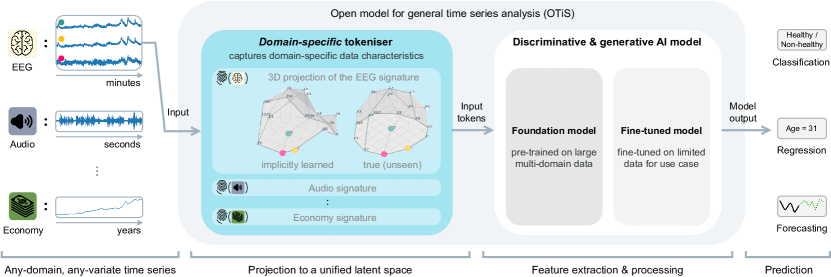
Figure 1: Overview of OTiS. Pre-trained on a large corpus of time series from diverse domains, OTiS enables general time series analysis. Its domain-specific tokeniser addresses time series heterogeneity across domains - including different numbers of variates, inter-variate relationships, temporal dynamics, and sampling frequencies - by learning unique domain signatures. After pre-training, the model can be fine-tuned on limited data from any domain, including previously unseen ones, to perform various tasks such as classification, regression, and forecasting.

Our key contributions can be summarised as follows:

1. We present OTiS, an open model for general time series analysis, with our entire pipeline and pre-trained weights publicly available at https://github.com/oetu/otis.

2. We propose a novel pre-training paradigm based on masked data modelling to address heterogeneity in multi-domain time series. Our approach includes a novel tokeniser with learnable signatures to capture domain-specific data characteristics, a dual masking strategy to learn temporal causality, and a normalised cross-correlation loss to model long-range dependencies.

3. We pre-train OTiS on a large corpus of publicly available time series from $8$ domains, spanning medicine, engineering, natural sciences, and finance. With $640,187$ samples and $11$ billion time points, this corpus represents diverse time series characteristics, enabling generalisable feature extraction.

4. We evaluate OTiS across $15$ downstream applications, including classification, regression, and forecasting. Our comprehensive analysis demonstrates that OTiS accurately captures domain-specific data characteristics and is competitive with both specialised and general state-of-the-art (SOTA) models, achieving new SOTA performance in $10$ tasks. Notably, none of the baselines is capable of performing all the tasks covered by OTiS.

2 Related Works

2.1 Self-Supervised Learning for Time Series

Time series vary significantly across domains, with differences in the number of variates, inter-variate relationships, temporal dynamics, and sampling frequencies. Due to this inherent heterogeneity, most existing works focus on pre-training models within a single domain (Oreshkin et al., 2019; Tang et al., 2020; Wu et al., 2021; Zhou et al., 2021; Wu et al., 2022a; Woo et al., 2022; Yue et al., 2022; Zhang et al., 2022; Li et al., 2023; Nie et al., 2023; Zeng et al., 2023; Dong et al., 2024). To develop more generalisable time series models, recent methods have explored multi-domain pre-training by addressing certain aspects of the heterogeneity, such as differences in variate count and sampling frequency. For instance, Liu et al. (2024) treat each variate in multi-variate time series independently to standardise generative tasks like forecasting, while Goswami et al. (2024) extend uni-variate analysis to discriminative tasks like classification. Similarly, Jiang et al. (2024) and Yang et al. (2024) standardise time series by cropping them into segments of predefined size and resampling them to a uniform frequency, respectively, to enable general classification capabilities in medical domains.

While partially addressing time series heterogeneity, these methods limit model capabilities for general time series analysis. Standardisation techniques like cropping or resampling may distort inter-variate relationships, temporal dynamics, and long-range dependencies. Additionally, many of these approaches are tailored to specific applications, such as generative tasks (Das et al., 2024; Liu et al., 2024; Woo et al., 2024), or focused on particular domains like medicine (Jiang et al., 2024; Yang et al., 2024). Moreover, recent foundational models (Das et al., 2024; Goswami et al., 2024; Liu et al., 2024) focus on uni-variate analysis, ignoring crucial inter-variate relationships essential for real-world applications, such as disease prediction (Schoffelen & Gross, 2009; Wu et al., 2022b). Our study aims to overcome these limitations by fully addressing heterogeneity of multi-domain time series, establishing a foundation for general time series analysis across domains and tasks.

2.2 Time Series Tokenisation

Transformers (Vaswani et al., 2017) have emerged as the preferred architecture for foundational models in NLP and CV due to their scalability (Kaplan et al., 2020; Gordon et al., 2021; Alabdulmohsin et al., 2022), enabling the training of models in the magnitude of $100$ billion parameters (Chowdhery et al., 2023; Touvron et al., 2023; Oquab et al., 2024; Ravi et al., 2024). To utilise a Transformer for time series analysis, a tokeniser is required to map the time series into a compact latent space. Current methods (Jin et al., 2023; Nie et al., 2023; Zhou et al., 2023; Das et al., 2024; Goswami et al., 2024; Jiang et al., 2024; Liu et al., 2024; Woo et al., 2024; Yang et al., 2024) follow established techniques from NLP and CV, dividing time series into patches of pre-defined size. These patches are then flattened into a $1$D sequence, with positional embeddings used to retain positional information. While uni-variate models (Nie et al., 2023; Das et al., 2024; Goswami et al., 2024; Liu et al., 2024) consider only temporal positions, multi-variate approaches (Woo et al., 2024; Yang et al., 2024; Jiang et al., 2024) account for both temporal and variate positions. However, none of these methods address the unique characteristics of variates, mistakenly assuming that the relationships between variates are identical across domains. Our work seeks to adapt the tokenisation process to preserve the domain-specific relationships between variates.

3 Methods

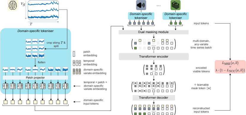
Figure 2: Architecture of OTiS. During pre-training, batches of time series from diverse domains are processed using a domain-specific tokeniser. This tokeniser splits a time series into fixed-size patches, which are then embedded using a patch projector shared across all variates and domains. A temporal embedding and a domain-specific variate embedding are added to each patch embedding. A dual masking strategy is employed to mask the resulting input tokens. The reconstruction of the multi-domain input tokens is guided using an auxiliary normalised cross-correlation (NCC) loss.

In this work, we present a novel multi-domain pre-training paradigm that enables generalisable feature extraction from large, heterogeneous time series corpora. We introduce a domain-specific tokeniser with learnable signatures to address heterogeneity in multi-domain time series, as described in Section 3.1. We tailor masked data modelling (MDM) for multi-domain time series to pre-train our open model for general time series analysis (OTiS) on a large, heterogeneous corpus, as detailed in Section 3.2. In particular, we propose normalised cross-correlation as a loss term to capture global temporal dynamics in time series, as explained in Section 3.3. Moreover, we introduce a dual masking strategy to capture bidirectional relationships and temporal causality, essential for general time series analysis, as described in Section 3.4. After pre-training, we fine-tune OTiS on limited data to perform a variety of downstream tasks in any - including previously unseen - domain, as outlined in Section 3.5. A graphical visualisation of our method is provided in Figure 2.

3.1 Domain-Specific Tokeniser

Overview.

Assume a time series sample $\displaystyle{\bm{X}}\in\mathbb{R}^{V_{S}\times T}$ from domain $S$, where $V_{S}$ denotes the number of variates specific to $S$ and $T$ denotes the number of time points. We randomly crop or zero-pad $\displaystyle{\bm{X}}$ to a fixed context length of $\overline{T}$ time points. We then split it into $T^{\prime}$ temporal patches of size $P$ along the time dimension, resulting in $V_{S}\cdot T^{\prime}$ patches $\displaystyle{\bm{x}}_{v,t}\in\mathbb{R}^{1\times P}$, where $v\in\{1,\dots,V_{S}\}$ and $t\in\{1,\dots,T^{\prime}\}$.

Next, we embed these patches using a shared patch projector across all variates and domains, resulting in patch embeddings $e^{\mathcal{P}}(\displaystyle{\bm{x}}_{v,t})=\displaystyle{\bm{e}}^{\mathcal{P}}_{v,t}\in\mathbb{R}^{1\times D}$, where $D$ denotes the model dimension. The patch projector consists of a $1$D convolutional layer followed by layer normalisation and GELU activation.

The permutation-equivariant nature of Transformers (Vaswani et al., 2017) requires the use of positional embeddings to accurately capture the inherent relationships in the input data. Initially introduced for $1$D textual token sequences (Vaswani et al., 2017), positional embeddings simply introduce an ordering into the input sequence. Modern implementations further extend their capabilities to encode more complex geometric information, such as $2$D spatial (Dosovitskiy et al., 2021) or graph (Kreuzer et al., 2021) structures. For the analysis of any-variate time series, we distinguish between the temporal and variate structure. The temporal structure is equivalent to a sequential $1$D structure, such that we use standard $1$D sinusoidal embeddings $e^{\mathcal{T}}(\displaystyle{\bm{x}}_{v,t})=\displaystyle{\bm{e}}^{\mathcal{T}}_{t}\in\mathbb{R}^{1\times D}$.

The variate structure exhibits great heterogeneity across domains. In domains with uni-variate and two-variate data, such as mono and stereo audio, the structure is either trivial or only requires a basic distinction between variates. In other domains, however, the variate structure may represent more complex relationships, such as $3$D manifolds for electroencephalography (EEG) or electrocardiography (ECG) data, or be of non-spatial nature, such as for financial data. Hence, we introduce learnable domain-specific variate embeddings to adequately address the heterogeneity across domains. These embeddings, denoted as $e^{\mathcal{V}}_{\mathcal{S}}(\displaystyle{\bm{x}}_{v,t})=\displaystyle{\bm{e}}^{\mathcal{V}}_{\mathcal{S},v}\in\mathbb{R}^{1\times D}$ for each variate $v$ in domain $S$, are designed to model the unique properties of a domain. They capture the inter-variate relationships and temporal dynamics specific to domain $S$, forming what can be considered as the signature of the very domain.

Finally, the patch, temporal, and domain-specific variate embeddings are summed to form the input token $\displaystyle{\bm{e}}_{v,t}=\displaystyle{\bm{e}}^{\mathcal{P}}_{v,t}+\displaystyle{\bm{e}}^{\mathcal{T}}_{t}+\displaystyle{\bm{e}}^{\mathcal{V}}_{\mathcal{S},v}\in\mathbb{R}^{1\times D}$. These input tokens collectively constitute the final input sequence $\displaystyle{\bm{E}}\in\mathbb{R}^{(V_{S}\cdot T^{\prime})\times D}$. To support batches of any-variate time series from multiple domains, we pad the variate dimension to the maximum number of variates in a batch $\overline{V}=\max_{S}V_{S}$. For samples where $V_{S}<\overline{V}$ or $T<\overline{T}$, attention masking is used to ensure that padded variate or temporal tokens are ignored. The domain-specific tokeniser is trained end-to-end with the Transformer layers.

Definition of (Sub-)Domains.

The domain-specific tokeniser is designed to integrate different datasets within a domain. Consider two EEG datasets, TDBrain (Van Dijk et al., 2022) and SEED (Zheng & Lu, 2015), which share $19$ identical variates but have different sampling frequencies of $500\,$Hz and $200\,$Hz, respectively. In this case, a single EEG-specific tokeniser ($V_{\text{EEG}}=19$) is sufficient to accommodate both sampling frequencies, i.e. $\displaystyle{\bm{E}}^{\mathcal{V}}_{\text{EEG-TDBrain}}=\displaystyle{\bm{E}}^{\mathcal{V}}_{\text{EEG-SEED}}=[\displaystyle{\bm{e}}^{\mathcal{V}}_{\text{EEG},1},\dots,\displaystyle{\bm{e}}^{\mathcal{V}}_{\text{EEG},19}]^{\top}\in\mathbb{R}^{19\times D}$, as demonstrated in our experiments in Section 4. Note that while these positional embeddings are agnostic to variate ordering, we simplify processing by aligning the variate order across datasets within the same domain. Consider another EEG dataset, LEMON (Babayan et al., 2019), which includes $62$ electrodes. Of these, $15$ overlap with the electrodes in TDBrain (Van Dijk et al., 2022) and SEED (Zheng & Lu, 2015), while the remaining $47$ are unique to LEMON (Babayan et al., 2019). In this scenario, the EEG-specific tokeniser can be extended by the $47$ new variates ($V_{\text{EEG}}=66$), such that $\displaystyle{\bm{E}}^{\mathcal{V}}_{\text{EEG-LEMON}}=[\displaystyle{\bm{e}}^{\mathcal{V}}_{\text{EEG},1},\dots,\displaystyle{\bm{e}}^{\mathcal{V}}_{\text{EEG},15},\displaystyle{\bm{e}}^{\mathcal{V}}_{\text{EEG},20},\dots,\displaystyle{\bm{e}}^{\mathcal{V}}_{\text{EEG},66}]^{\top}\in\mathbb{R}^{62\times D}$. In this way, different datasets can be combined to approximate the underlying data distribution of a domain $S$, e.g. EEG, enabling the creation of large and diverse time series corpora.

Multi-Variate or Uni-Variate Analysis?

Consider the Electricity dataset (UCI, 2024), which contains electricity consumption data for $321$ households recorded from $2012$ to $2014$. These $321$ observations are sampled from an underlying population and are assumed to be independent and identically distributed (i.i.d.). In this scenario, we perform a uni-variate analysis ($V_{\text{Electricity}}=1$) of the data, initialising a single Electricity-specific variate embedding that models the hourly consumption of a household. In contrast, the Weather dataset (Wetterstation, 2024) contains $21$ climatological indicators, such as air temperature, precipitation, and wind speed, which are not i.i.d. because they directly interact and correlate with one another. Therefore, a multi-variate analysis ($V_{\text{Weather}}=21$) is conducted to account for the dependencies and interactions between the observations.

3.2 Pre-Training on Multi-Domain Time Series

We pre-train our model using masked data modelling (MDM) (He et al., 2022) to learn generalisable time series features across domains. We mask a subset of input tokens and only encode the visible (i.e. non-masked) tokens using an encoder $f(\cdot)$. Afterwards, we complement the encoded tokens with learnable mask tokens and feed them to a decoder $g(\cdot)$, reconstructing the original input tokens.

More precisely, we draw a binary mask $\displaystyle{\bm{m}}\in\{0,1\}^{V_{S}\cdot T^{\prime}}$, following the dual masking strategy proposed in Section 3.4, and apply it to the input sequence $\displaystyle{\bm{E}}\in\mathbb{R}^{(V_{S}\cdot T^{\prime})\times D}$. Thus, we obtain a visible view $\displaystyle{\bm{E}}[\displaystyle{\bm{m}}]\in\mathbb{R}^{N_{1}\times D}$, where $N_{1}=\sum_{v=1}^{V_{S}}\sum_{t=1}^{T^{\prime}}m_{v,t}$ and $N_{0}=(V_{S}\cdot T^{\prime})-N_{1}$ denote the number of visible and masked tokens, respectively. The visible view $\displaystyle{\bm{E}}[\displaystyle{\bm{m}}]$ is then fed to the encoder $f(\cdot)$ to compute the token features $\displaystyle{\bm{H}}\in\mathbb{R}^{N_{1}\times D}$:

$${\bm{H}}=f(\displaystyle{\bm{E}}[\displaystyle{\bm{m}}]).$$ (1)

To reconstruct the original input, these token features are fed to the decoder $g(\cdot)$ together with a special, learnable mask token $\displaystyle{\bm{e}}^{\mathcal{M}}\in\mathbb{R}^{1\times D}$, that is inserted at the masked positions where $m_{v,t}=0$:

$${\bm{h}}^{\prime}_{v,t}=\begin{cases}\displaystyle{\bm{h}}_{v,t}&\text{if }m_{v,t}=1\\ \displaystyle{\bm{e}}^{\mathcal{M}}&\text{if }m_{v,t}=0\end{cases},$$ (2)

such that $\displaystyle{\bm{H}}^{\prime}\in\mathbb{R}^{(V_{S}\cdot T^{\prime})\times D}$. The decoder $g(\cdot)$ then predicts the reconstructed input $\displaystyle\widehat{{\bm{X}}}\in\mathbb{R}^{V_{S}\times(T^{\prime}\cdot P)}$:

$$\widehat{{\bm{X}}}=g(\displaystyle{\bm{H}}^{\prime}),$$ (3)

where $(T^{\prime}\cdot P)=\overline{T}$, i.e. the context length specified in time points. Eventually, the domain-specific tokeniser described in Section 3.1, the encoder $f(\cdot)$, and the decoder $g(\cdot)$ are optimised end-to-end using the mean squared error (MSE) loss on all reconstructed input tokens:

$$\mathcal{L}_{\text{MSE}}=\frac{1}{V_{S}\cdot T^{\prime}}\sum_{v=1}^{V_{S}}\sum_{t=1}^{T^{\prime}}\|\displaystyle{\bm{x}}_{v,t}-\displaystyle\widehat{{\bm{x}}}_{v,t}\|_{2}^{2}.$$ (4)

3.3 Normalised Cross-Correlation Loss

MDM focuses on reconstructing masked parts of the data, emphasising local patterns through the MSE loss (4). However, time series often exhibit long-range dependencies, where past values influence future outcomes over extended periods. To accurately capture these global patterns, we introduce normalised cross-correlation (NCC) as a loss term in MDM for time series:

$$\mathcal{L}_{\text{NCC}}=\frac{1}{V_{S}\cdot\overline{T}}\sum^{V_{S}}_{v=1}\sum^{\overline{T}}_{t=1}\hskip 2.84526pt\frac{1}{\sigma_{\displaystyle{\bm{x}}_{v}}\sigma_{\displaystyle\widehat{{\bm{x}}}_{v}}}(x_{v,t}-\mu_{\displaystyle{\bm{x}}_{v}})(\widehat{x}_{v,t}-\mu_{\displaystyle\widehat{{\bm{x}}}_{v}})\in\left[-1,1\right],$$ (5)

where $\mu$ and $\sigma$ denote the mean and standard deviation, respectively. Hence, to capture both local and global temporal dynamics, the total loss used to optimise OTiS is defined as

$$\mathcal{L}=\mathcal{L}_{\text{MSE}}+\lambda\cdot\left(1-\mathcal{L}_{\text{NCC}}\right),$$ (6)

where $\lambda$ is empirically set to $0.1$ during pre-training.

3.4 Dual Masking Strategy

We design the masking strategy to enhance foundational model capabilites in time series analysis. Specifically, we randomly select between two masking schemes during pre-training, namely random masking and post-fix masking. In $75\,$% of cases, we apply random masking, where each $m_{v,t}$ is independently sampled from a Bernoulli distribution with probability $p=1-\rho$, with $\rho$ denoting the masking ratio (i.e. $m_{v,t}\sim\text{Bernoulli}(1-\rho)$). This encourages the model to learn complex inter-variate relationships across the entire time series. In the remaining $25\,\%$ of cases, we employ post-fix masking, which masks the second half of the temporal dimension, leaving only the first half visible (i.e. $m_{v,t}=\mathbbm{1}_{[t\leq T^{\prime}/2]}$). The prediction of future values solely based on past observations simulates real-world forecasting conditions, helping the model to capture temporal causality. Overall, this dual masking strategy enables OTiS to learn both bidirectional relationships and temporal causality, which are essential for general time series analysis.

3.5 Fine-Tuning & Inference on (Unseen) Target Domains

Inclusion of Unseen Domains.

For a new domain $S$, a randomly initialised variate embedding $\displaystyle{\bm{E}}^{\mathcal{V}}_{\mathcal{S}}\in\mathbb{R}^{V_{S}\times D}$ is introduced. The domain-specific tokeniser is then fine-tuned alongside the encoder $f(\cdot)$, and, if required, the decoder $g(\cdot)$, for the specific downstream task, as described in the following.

Classification & Regression.

We use the encoder $f(\cdot)$ and the unmasked input sequence $\displaystyle{\bm{E}}$ to compute all token features $\displaystyle{\bm{H}}=f(\displaystyle{\bm{E}})\in\mathbb{R}^{(V_{S}\cdot T^{\prime})\times D}$. We average-pool these features into a global token $\displaystyle{\bm{h}}^{*}\in\mathbb{R}^{1\times D}$, which we feed through a linear layer to obtain the final model prediction. We optimise a cross-entropy and MSE loss for the classification and regression tasks, respectively.

Forecasting.

We apply post-fix masking to generate a binary mask $\displaystyle{\bm{m}}\in\{0,1\}^{V_{S}\cdot T^{\prime}}$ for the forecasting task. The encoder $f(\cdot)$ is used to compute the visible token features $\displaystyle{\bm{H}}\in\mathbb{R}^{N_{1}\times D}$. We then concatenate the sequence with learnable mask tokens to form $\displaystyle{\bm{H}}^{\prime}\in\mathbb{R}^{(V_{S}\cdot T^{\prime})\times D}$, which is passed through the decoder $g(\cdot)$ to produce the final output. We optimise the MSE loss together with the NCC loss term over all reconstructed input tokens.

4 Experiments & Results

4.1 Model Variants and Implementation Details

We introduce OTiS in three different configurations, Base, Large, and Huge, with their specific architectures described in Appendix C.1, to explore scaling laws with respect to the model size. We set the patch size and stride to $P=24$, respectively, to split the time series into $T^{\prime}=\frac{\overline{T}}{P}$ non-overlapping patches along the time dimension. For pre-training, the context length specified in time points is set to $\overline{T}=1008$, resulting in $T^{\prime}=42$ sinusoidal temporal embeddings. If longer context lengths are required during fine-tuning, these embeddings are linearly interpolated (i.e. $T^{\prime}_{\text{ft}}\geq 42$) to offer greater flexibility for downstream applications. We tune the hyperparameters for pre-training and fine-tuning as described in Appendix C. An overview of the computational costs is provided in Appendix D.

4.2 Large and Diverse Pre-Training Corpus

We aim to develop a general time series model that fully handles the heterogeneity in real-world data. Specifically, our model is designed to handle time series with different variate counts $V_{S}$, inter-variate relationships, temporal dynamics, and sampling frequency, ensuring flexibility for downstream tasks. To this end, we pre-train our model on a large and diverse corpus of publicly available data spanning $8$ domains, with a total of $640,187$ samples and $11$ billion time points, as summarised in Table 1. A detailed description of the datasets included in our pre-training corpus can be found in Appendix A. The time series corpus is split into $612,394$ training and $27,793$ validation samples for pre-training.

Table 1: Overview of our large and diverse pre-training corpus. The corpus is built with unlabelled data from eight domains, encompassing medicine, engineering, natural sciences, and finance.

Domain	Name	Samples	Variates	Time points	Frequency	Disk size
$S$			$V_{S}$
ECG	MIMIC-IV-ECG 2023	$400,000$	$12$	$5,000$	$500\,$Hz	$90\,$GB
Temperature	DWD 2024	$203,340$	$1$	$720$	(hourly) $278\,$mHz	$614\,$MB
Audio (stereo)	AudioSet-$20$K 2017	$16,123$	$2$	$441,000$	$44.1\,$kHz	$53\,$GB
Audio (mono)	AudioSet-$20$K 2017	$3,491$	$1$	$441,000$	$44.1\,$kHz	$6\,$GB
Electromechanics	FD-A 2016	$13,640$	$1$	$5,120$	$64\,$kHz	$161\,$MB
EEG	TDBrain 2022	$2,692$	$19$	$60,000$	$500\,$Hz	$12\,$GB
EEG	SEED 2015	$675$	$19$	$37,000$	$200\,$Hz	$2\,$GB
Banking	NN$5$ 2012	$111$	$1$	$971$	(daily) $12\,\mu$Hz	$370\,$KB
Economics	FRED-MD 2016	$107$	$1$	$728$	(monthly) $386\,$nHz	$330\,$KB
Economics	Exchange 2018	$8$	$1$	$7,588$	(daily) $12\,\mu$Hz	$240\,$KB
		640,187		11,052,756,981		164 GB

4.3 Benchmarking Across Domains and Tasks

To assess the utility of OTiS in real-world settings, we conduct experiments on three key use cases in time series analysis: classification, regression, and forecasting. For classification, we perform binary epilepsy detection using EEG (Epilepsy 2001), multi-class fault detection in rolling bearings from vibration signals (FD-B 2016), multi-class hand-gesture classification with accelerometer signals (Gesture 2009), and multi-class muscular disease classification using electromyographie (EMG 2000). In regression, we predict five imaging-derived cardiac phenotypes from $12$-lead ECG (LVEDV, LVESV, LVSV, LVEF, LVM 2020). For forecasting, we predict electricity transformer temperature (ETT 2021), weather (Weather 2024), and electricity consumption (Electricity 2024). Further dataset details are provided in Appendix B. We adhere to the established data splitting and evaluation procedures for the classification (Zhang et al., 2022), regression (Turgut et al., 2023), and forecasting (Zhou et al., 2021) tasks. All experiments are reported as mean and standard deviation across five seeds set during fine-tuning.

Table 2: Classification and regression performance on a total of $9$ benchmark tasks. OTiS is competitive with specialised baselines, setting new state-of-the-art on $6$ tasks and even outperforming the multimodal CM-AE and MMCL. This demonstrates the capability of OTiS to extract high-level semantics. Best score in bold, second best underlined. ^∙ indicates tasks in previously unseen domains.

(a) Classification [Accuracy (ACC¹$\uparrow$) in %]

Model	Epilepsy	FD-B	Gesture∙	EMG∙
SimCLR 2020	90.71	49.17	48.04	61.46
CoST 2022	88.40	47.06	68.33	53.65
TS2Vec 2022	93.95	47.90	69.17	78.54
TF-C 2022	94.95	69.38	76.42	81.71
Ti-MAE 2023	89.71	60.88	71.88	69.99
SimMTM 2024	95.49	69.40	80.00	97.56
OTiS-Base	94.25	99.24	63.61	97.56
OTiS-Large	94.03	98.62	62.50	98.37
OTiS-Huge	91.48	98.32	63.61	98.37

(b) Regression [R-squared ($R^{2}$ $\uparrow$)]

Model	LVEDV	LVESV	LVSV	LVEF	LVM
ViT 2023	0.409	0.396	0.299	0.175	0.469
MAE 2023	0.486	0.482	0.359	0.237	0.573
CM-AE* 2023	0.451	0.380	0.316	0.103	0.536
MMCL* 2023	0.504	0.503	0.370	0.250	0.608
OTiS-Base	0.509	0.512	0.391	0.292	0.592
OTiS-Large	0.504	0.503	0.371	0.267	0.592
OTiS-Huge	0.505	0.510	0.376	0.281	0.593
* Models that incorporate paired imaging data during pre-training.

OTiS demonstrates strong classification capabilities, setting two new benchmarks, as shown in Table 2(a). Additionally, OTiS excels in predicting imaging-derived cardiac phenotypes, even surpassing multimodal baselines that incorporate imaging data during pre-training, as summarised in Table 2(b). Our model outperforms the baselines in $4$ out of $5$ regression tasks. As shown in Table 3, OTiS also exhibits strong forecasting capabilities, outperforming current models in $4$ out of $6$ benchmarks. Notably, all of the forecasting tasks are performed in previously unseen domains. A visualisation of the forecast predictions can be found in Appendix F. Overall, OTiS outperforms both specialised and general state-of-the-art baselines in $10$ out of $15$ diverse applications across $8$ domains, demonstrating its strong utility and generalisability across (unseen) domains and tasks.

Table 3: Forecasting performance on $6$ benchmark tasks. OTiS is competitive with specialised and general baselines, setting new state-of-the-art on $4$ tasks and showcasing its ability to capture local time series features. A forecasting horizon of $96$ time points is predicted from the past $336$ (*$512$, ${}^{+}904$) time points. Mean squared error (MSE $\downarrow$) is reported. Best score in bold, second best underlined. ^∙ indicates tasks in previously unseen domains.

Model	ETTh1∙	ETTh2∙	ETTm1∙	ETTm2∙	Weather∙	Electricity∙
N-BEATS 2019	0.399	0.327	0.318	0.197	0.152	0.131
Autoformer 2021	0.435	0.332	0.510	0.205	0.249	0.196
TimesNet 2022a	0.384	0.340	0.338	0.187	0.172	0.168
DLinear 2023	0.375	0.289	0.299	0.167	0.176	0.140
PatchTST 2023	0.370	0.274	0.293	0.166	0.149	0.129
Time-LLM 2023	0.408	0.286	0.384	0.181	†	†
GPT4TS 2023	0.376	0.285	0.292	0.173	0.162	0.139
MOMENT* 2024	0.387	0.288	0.293	0.170	0.154	0.136
MOIRAI+ 2024	0.375	0.277	0.335	0.189	0.167	0.152
OTiS-Base	0.424	0.212	0.337	0.161	0.139	0.128
OTiS-Large	0.446	0.205	0.362	0.173	0.142	0.127
OTiS-Huge	0.461	0.215	0.384	0.181	0.149	0.132
† Experiments could not be conducted on a single NVIDIA RTX A$6000$-$48$GB GPU.

4.4 Domain Signature Analysis

A key component of OTiS is its use of domain-specific variate embeddings. While these embeddings are randomly initialised, we expect them to capture unique domain characteristics during training, eventually serving as the signature of their respective domain. To validate this hypothesis, we analyse the domain-specific variate embeddings after pre-training using principal component analysis (PCA).

First, we find that OTiS unifies time series from diverse domains into a meaningful latent space, where embeddings of domains with shared high-level semantics cluster together, as depicted in Appendix E.1. For example, embeddings of mono and stereo audio group closely, as do those of banking and economics. Moreover, EEG-specific embeddings are clearly separated and ECG-specific embeddings form a tight cluster.

Second, OTiS preserves low-level semantics specific to each domain, such as the relationships between variates. To explore this, we focus on the learned variate embeddings of EEG, the most complex domain in our corpus. EEG variates correspond to actual electrodes, each associated with a $3$D position in space or a $2$D position on the scalp, which is ideal for studying inter-variate relationships. Our analysis covers both (i) variate embeddings for $10$-$20$ system EEG recordings with $19$ electrodes learned during multi-domain pre-training, and (ii) variate embeddings for previously unseen EEG recordings with $32$ electrodes learned during fine-tuning of the pre-trained OTiS. We find that the first three principal components explain (i) $74.7\,\%$ and (ii) $87.9\,\%$ of the variance, indicating that the $3$D PCA projections of the variate embeddings correspond closely to the actual electrode positions. A visualisation of the learned $3$D electrode layout is provided in Appendix E. Additionally, we linearly align these positions with the true EEG electrode layout on the $2$D scalp manifold, as depicted in Figure 3. The alignment yields $R^{2}$ values of (i) $0.81$ and (ii) $0.95$, confirming a strong correspondence between the learned variate embeddings and the actual electrode layout.

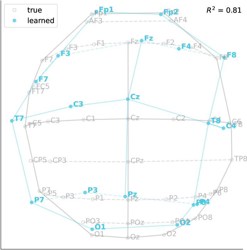
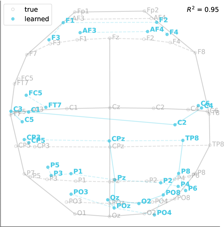
Figure 3: $2$D PCA projections of the learned EEG-specific variate embeddings, overlaid on the actual EEG electrode layout. (Left) Embeddings for $10$-$20$ system EEG recordings with $19$ electrodes learned during pre-training. (Right) Embeddings for previously unseen EEG recordings with $32$ electrodes learned during fine-tuning. The embeddings accurately reflect the spatial electrode layout, as confirmed by high correlations (R²) between the PCA projections $\bullet$ and the true layout $\circ$.

4.5 Scaling Study

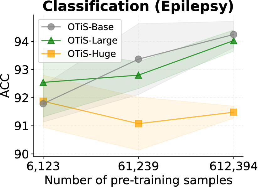
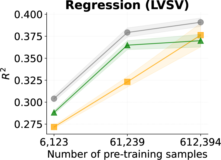
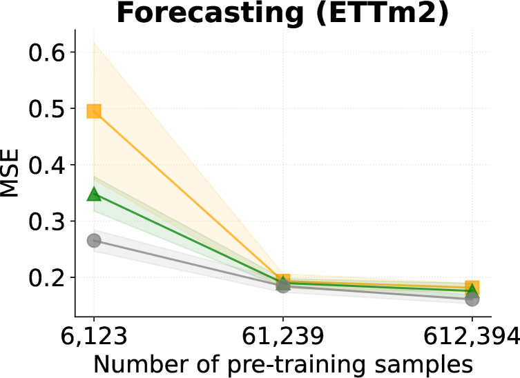
Figure 4: Performance of OTiS with different numbers of pre-training samples. Shaded regions indicate the standard deviation across $5$ seeds. Increasing dataset size generally improves downstream performance. Scaling model size requires even larger pre-training corpora to be effective.

We analyse the scaling behaviour of OTiS with respect to model and dataset size. To this end, we subsample the pre-training data to $10\,\%$ and $1\,\%$ of its original size, ensuring that each subset is fully contained within the corresponding superset. We evaluate the downstream performance of all OTiS variants across classification, regression, and forecasting tasks, as depicted in Figure 4.

The experiments demonstrate that downstream performance generally scales with dataset size, achieving the best results with the full pre-training dataset. This trend, however, does not directly apply to model size, which is in line with the scaling behaviour observed in current time series foundational models (Woo et al., 2024; Goswami et al., 2024). Given that performance generally improves across all models with increasing data size, we hypothesise that scaling the model size could prove beneficial with even larger pre-training corpora.

4.6 Ablation Study

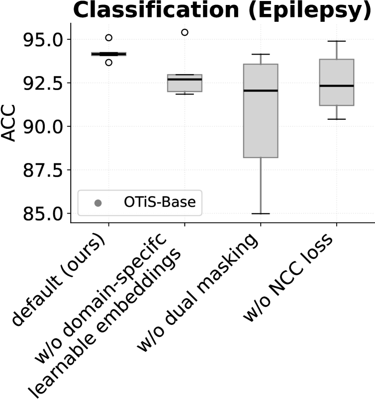
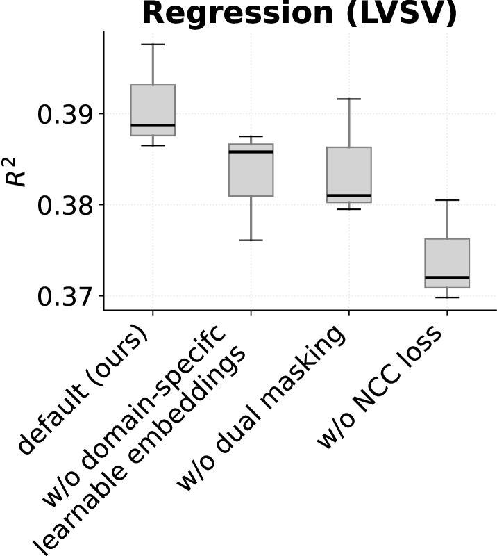
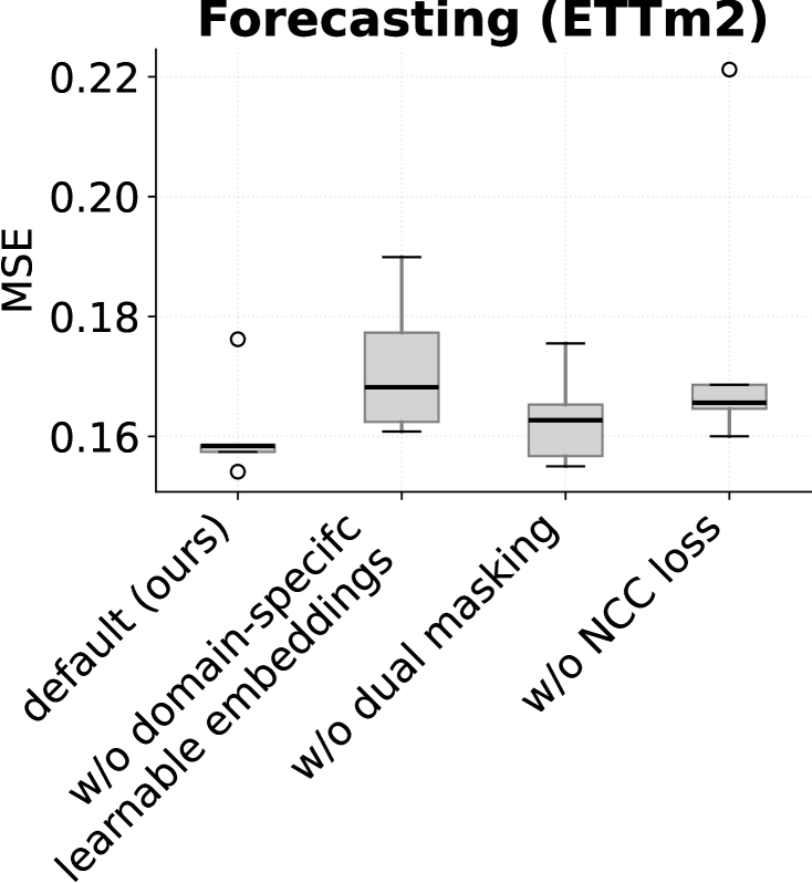
Figure 5: Ablation study on key components of OTiS. Downstream performance is analysed across $5$ seeds. A leave-one-out approach is used to evaluate the influence of each component. The default setting, which includes all components, demonstrates superior model capabilities across tasks.

We perform an ablation study to analyse the impact of OTiS’ key components: the domain-specific tokeniser, dual masking strategy, and normalised cross-correlation (NCC) loss. As shown in Figure 5, the best and most robust performance is achieved when all components are used during pre-training.

Replacing the domain-specific variate embeddings with domain-agnostic embeddings (i.e. learnable embeddings shared across all domains) consistently led to inferior performance across all tasks, demonstrating the importance of capturing domain-specific data characteristics during tokenisation. Switching from dual masking to random masking resulted in performance degradation, although the impact was less notable for generative tasks than for discriminative tasks. We hypothesise that the NCC loss already captures temporal causality, which is particularly crucial for generative tasks like forecasting. Overall, removing the NCC loss caused performance declines across all downstream tasks, emphasising the role of long-range dependencies for general time series understanding.

5 Discussion & Conclusion

In this study, we explore the problem of effective pre-training on heterogeneous time series corpora. Time series vary substantially across domains, e.g. with respect to inter-variate relationships and temporal dynamics, rendering generalisable feature extraction from multi-domain time series difficult. To address this issue, we present OTiS, an open model for general time series analysis, specifically designed to handle multi-domain heterogeneity. Our novel multi-domain pre-training paradigm, including a domain-specific tokeniser with learnable signatures, a dual masking strategy, and a normalised cross-correlation (NCC) loss, enables OTiS to extract generalisable time series features.

In extensive experiments, we demonstrate that OTiS generalises well across $15$ diverse downstream applications spanning $8$ distinct domains, achieving competitive performance with both specialised and general state-of-the-art (SOTA) models. In a qualitative analysis, we further show that OTiS unifies time series from diverse domains in a meaningful latent space, while preserving low-level semantics of a domain including the inter-variate relationships. Thereby, our work establishes a strong foundation for future advancements in interpretable and general time series analysis.

Limitations.

While OTiS outperforms SOTA models across $10$ tasks, our experiments in low-data regimes suggest that larger pre-training corpora could further enhance its performance. Unlike in NLP and CV, where large datasets are curated from web-crawled data, foundational models in time series, including OTiS, still rely on manually curated datasets. Future work could explore fully automatic pipelines, e.g. using embedding similarity, to filter and rebalance multi-domain time series from the web. OTiS could further benefit from processing domain signatures during inference, potentially unlocking zero-shot capabilities, similarly to those seen in foundational models in NLP and CV.

Appendix A Large Multi-Domain Pre-Training Corpus

In this section, we present an overview of our large and diverse pre-training corpus. The corpus consists of publicly available data spanning eight domains, with a total of $640,187$ samples and $11$ billion time points. In the following, we provide a detailed breakdown of the domains and the datasets they encompass. Note that we apply channel-wise standard normalisation to the datasets unless otherwise specified.

ECG.

The MIMIC-IV-ECG dataset (Gow et al., 2023) contains diagnostic $10$-second, $12$-lead ECG recordings sampled at a frequency of $500$ Hz. While the entire dataset comprises $800,035$ samples, we include only the first half of the recordings available in the database, preventing the ECG data from predominating in the pre-training corpus. To remove the baseline drift from the ECG data, we use the asymmetric least square smoothing technique (Zhang et al., 2010). Note that we apply standard normalisation separately to the Einthoven, Goldberger, and Wilson leads.

Temperature.

The Deutscher Wetterdienst (DWD) dataset (Wetterdienst, 2024) contains hourly air temperature measurements from $629$ weather stations across Germany. Since the recording length varies significantly, ranging from $763$ to $1,148,290$ hours per station, we split the data into chunks of $720$ hours (approximately one month).

Audio.

The AudioSet dataset (Gemmeke et al., 2017) contains $10$-second YouTube clips for audio classification, featuring $527$ types of audio events that are weakly annotated for each clip. The full training set includes a class-wise balanced subset (AudioSet-$20$K, $22,176$ clips) and an unbalanced (AudioSet-$2$M $2,042,985$ clips) set. For our pre-training corpus, we use the balanced AudioSet-$20$K, which contains $3,491$ mono and $16,123$ stereo recordings, all sampled at $44,100\,$Hz.

Electromechanics.

The FD-A dataset (Lessmeier et al., 2016) collects vibration signals from rolling bearings in a mechanical system for fault detection purposes. Each sample consists of $5,120$ timestamps, indicating one of three mechanical device states. Note that the FD-B dataset is similar to FD-A but includes rolling bearings tested under different working conditions, such as varying rotational speeds.

EEG.

The TDBrain dataset (Van Dijk et al., 2022) includes raw resting-state EEG data from $1,274$ psychiatric patients aged $5$ to $89$, collected between $2001$ and $2021$. The dataset covers a range of conditions, including Major Depressive Disorder ($426$ patients), Attention Deficit Hyperactivity Disorder ($271$ patients), Subjective Memory Complaints ($119$ patients), and Obsessive-Compulsive Disorder ($75$ patients). The data was recorded at $500\,$Hz using $26$ channel EEG-recordings, based on the $10$-$10$ electrode international system.

The SEED dataset (Zheng & Lu, 2015) contains EEG data recorded under three emotional states: positive, neutral, and negative. It comprises EEG data from $15$ subjects, with each subject participating in experiments twice, several days apart. The data is sampled at $200\,$Hz and recorded using $62$ channel EEG-recordings, based on the $10$-$20$ electrode international system.

For simplicity, we only consider the $19$ channels common to both datasets, i.e. the channels that correspond to the $10$-$20$ electrode international system.

Banking.

The NN$5$ competition dataset (Taieb et al., 2012) consists of daily cash withdrawals observed at $111$ randomly selected automated teller machines across various locations in England.

Economics.

The FRED-MD dataset (McCracken & Ng, 2016) contains $107$ monthly time series showing a set of macro-economic indicators from the Federal Reserve Bank of St Louis. The data was extracted from the FRED-MD database.

The Exchange dataset (Lai et al., 2018) records the daily exchange rates of eight different nations, including Australia, Great Britain, Canada, Switzerland, China, Japan, New Zealand, and Singapore, ranging from $1990$ to $2016$.

Appendix B Benchmark Dataset Details

We provide an overview of the datasets used to benchmark our model on $15$ distinct downstream applications in Table 4. Our benchmarking experiments include classifcation, regression, and forecasting tasks.

Table 4: Experimental setup with all conducted downstream applications, evaluation metrics, and datasets used for benchmarking.

Task	Metric	Dataset
		Domain	Name	Samples	Variates	Time points	Frequency
		$S$			$V_{S}$
Classification	ACC	EEG	Epilepsy 2001	$11,500$	$1$	$178$	$174\,$Hz
		Electromechanics	FD-B 2016	$13,640$	$1$	$5,120$	$64\,$kHz
		Acceleration	Gesture 2009	$560$	$3$	$206$	$100\,$Hz
		EMG	EMG 2000	$204$	$1$	$1,500$	$4\,$kHz
Regression	$R^{2}$	ECG	UK BioBank 2015	$18,926$	$12$	$5,000$	$500\,$Hz
Forecasting	MSE	Energy	ETTh1 2021	$1$	$7$	$17,420$	(hourly) $278\,$mHz
			ETTh2 2021	$1$	$7$	$17,420$	(hourly) $278\,$mHz
			ETTm1 2021	$1$	$7$	$69,680$	(minutely) $1.1\,$mHz
			ETTm2 2021	$1$	$7$	$69,680$	(minutely) $1.1\,$mHz
		Weather	Weather 2024	$1$	$21$	$52,696$	(minutely) $2.8\,$mHz
		Electricity	Electricity 2024	$321$	$1$	$26,304$	(hourly) $278\,$mHz

Appendix C Experiment Details

C.1 Model Variants

To explore the scaling laws with respect to the model size, we provide OTiS in three variants, as summerised in Table 5.

Table 5: Details of model variants.

Model	Layers	Hidden size D	MLP size	Heads	$d_{kv}$	Parameters
OTiS-Base	$12$	$192$	$768$	$3$	$64$	$8\,$M
OTiS-Large	$18$	$384$	$1536$	$6$	$64$	$44\,$M
OTiS-Huge	$24$	$576$	$2304$	$8$	$72$	$131\,$M

C.2 Pre-Training & Fine-Tuning Parameters

We provide the hyperparameters used to pre-train all variants of OTiS in Table 6. The hyperparameters used to fine-tune our models for the classification, regression, and forecasting tasks are provided in Table 7, 8, and 9, respectively.

Table 6: Hyperparameters used for pre-training. Pre-training is performed on $4$ NVIDIA A$100$-$80$GB GPUs. A cosine learning rate scheduler is applied with a $10\,\%$ warmup. All OTiS configurations use a shallow decoder with $2\,$M parameters, consisting of $4$ layers with a hidden size of $160$, an MLP with size $640$, and $5$ heads.

Model	Epochs	Batch size	Base LR	LR decay	NCC $\lambda$	Mask ratio $\rho$	Weight decay
OTiS-Base	$200$	$5120$	$3$e-$5$	cosine	$0.1$	$0.75$	$0.10$
OTiS-Large	$200$	$3328$	$1$e-$5$	cosine	$0.1$	$0.75$	$0.15$
OTiS-Huge	$200$	$2880$	$3$e-$6$	cosine	$0.1$	$0.75$	$0.05$

Table 7: Hyperparameters used for fine-tuning the classification tasks on a single NVIDIA RTX A$6000$-$48$GB GPU. A cosine learning rate scheduler is applied with a $10\,\%$ warmup.

Dataset	Model	Epochs	Batch size	Base LR	Drop path	Layer decay	Weight decay	Label smoothing
Epilepsy	OTiS-Base	$75$	$32$	$1$e-$3$	$0.2$	$0.75$	$0.2$	$0.1$
	OTiS-Large	$75$	$32$	$3$e-$3$	$0.2$	$0.50$	$0.1$	$0.1$
	OTiS-Huge	$75$	$32$	$3$e-$3$	$0.0$	$0.75$	$0.2$	$0.2$
FD-B	OTiS-Base	$75$	$32$	$3$e-$4$	$0.0$	$0.75$	$0.1$	$0.1$
	OTiS-Large	$75$	$32$	$1$e-$3$	$0.1$	$0.75$	$0.1$	$0.2$
	OTiS-Huge	$75$	$32$	$3$e-$4$	$0.1$	$0.75$	$0.2$	$0.1$
Gesture	OTiS-Base	$75$	$32$	$1$e-$2$	$0.1$	$0.25$	$0.2$	$0.1$
	OTiS-Large	$75$	$32$	$3$e-$3$	$0.2$	$0.75$	$0.1$	$0.0$
	OTiS-Huge	$75$	$32$	$1$e-$2$	$0.0$	$0.75$	$0.1$	$0.1$
EMG	OTiS-Base	$75$	$32$	$1$e-$3$	$0.2$	$0.75$	$0.1$	$0.2$
	OTiS-Large	$75$	$32$	$3$e-$3$	$0.1$	$0.75$	$0.2$	$0.1$
	OTiS-Huge	$75$	$32$	$3$e-$3$	$0.1$	$0.75$	$0.2$	$0.2$

Table 8: Hyperparameters used for fine-tuning the regression tasks on a single NVIDIA RTX A$6000$-$48$GB GPU. A cosine learning rate scheduler is applied with a $10\,\%$ warmup.

Dataset	Model	Epochs	Batch size	Base LR	Drop path	Layer decay	Weight decay
UK BioBank	OTiS-Base	$50$	$192$	$3$e-$4$	$0.2$	$0.75$	$0.1$
	OTiS-Large	$50$	$160$	$1$e-$4$	$0.2$	$0.75$	$0.1$
	OTiS-Huge	$50$	$200$	$1$e-$4$	$0.2$	$0.75$	$0.1$

Table 9: Hyperparameters used for fine-tuning the forecasting tasks. A cosine learning rate scheduler is applied with a $10\,\%$ warmup.

Dataset	Model	Epochs	Batch size	Base LR	NCC $\lambda$	Weight decay
ETTh1	OTiS-Base	$1000$	$1$	$1$e-$0$	$0.1$	$0.15$
	OTiS-Large	$1000$	$1$	$1$e-$1$	$0.2$	$0.15$
	OTiS-Huge	$1000$	$1$	$3$e-$1$	$0.1$	$0.15$
ETTh2	OTiS-Base	$1000$	$1$	$1$e-$0$	$0.2$	$0.25$
	OTiS-Large	$1000$	$1$	$1$e-$1$	$0.1$	$0.25$
	OTiS-Huge	$1000$	$1$	$3$e-$1$	$0.0$	$0.25$
ETTm1	OTiS-Base	$1000$	$1$	$3$e-$1$	$0.2$	$0.25$
	OTiS-Large	$1000$	$1$	$3$e-$1$	$0.2$	$0.25$
	OTiS-Huge	$1000$	$1$	$1$e-$1$	$0.1$	$0.15$
ETTm2	OTiS-Base	$1000$	$1$	$3$e-$1$	$0.1$	$0.25$
	OTiS-Large	$1000$	$1$	$3$e-$1$	$0.2$	$0.25$
	OTiS-Huge	$1000$	$1$	$1$e-$1$	$0.2$	$0.25$
Weather	OTiS-Base	$1000$	$1$	$3$e-$1$	$0.2$	$0.15$
	OTiS-Large	$1000$	$1$	$3$e-$1$	$0.2$	$0.15$
	OTiS-Huge	$1000$	$1$	$1$e-$1$	$0.2$	$0.05$
Electricity	OTiS-Base	$250$	$32$	$3$e-$2$	$0.0$	$0.25$
	OTiS-Large	$250$	$32$	$3$e-$2$	$0.0$	$0.15$
	OTiS-Huge	$250$	$32$	$3$e-$2$	$0.2$	$0.15$

Appendix D Computation Costs

We provide an overview of the computational resources used to train OTiS in Table 10.

Table 10: Computational resources used to pre-train OTiS. Note that fine-tuning and inference of all OTiS variants on downstream applications were performed using a single NVIDIA RTX A$6000$-$48$GB and $32$ CPUs.

Model	Parameters	Power consumption	CPU count	GPU
				Count	Hours	Type
OTiS-Base	$8$ M	$700\,$W*	$128$	$4$	$115$†	NVIDIA A$100$-$80$GB
OTiS-Large	$44$ M	$800\,$W*	$128$	$4$	$154$†	NVIDIA A$100$-$80$GB
OTiS-Huge	$131$ M	$960\,$W*	$128$	$4$	$219$†	NVIDIA A$100$-$80$GB
* Total power consumption across all GPUs.
† Total hours across all GPUs.

Appendix E Domain Signature Analysis

To analyse the domain signatures, we reduce the dimensionality of the domain-specific variate embeddings by employing a principal component analysis (PCA). Our analysis shows that OTiS unifies time series from diverse domains into a meaningful latent space, while accurately capturing the inter-variate relationships within a domain.

E.1 Inter-Domain Analysis

A visualisation of all domain-specific variate embeddings learned during pre-training is provided in Figure 6. We find that OTiS learns a meaningful latent space, where embeddings of domains with shared high-level semantics cluster closely together.

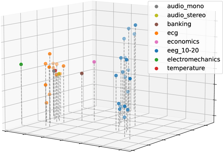
(a) $3$D projection.

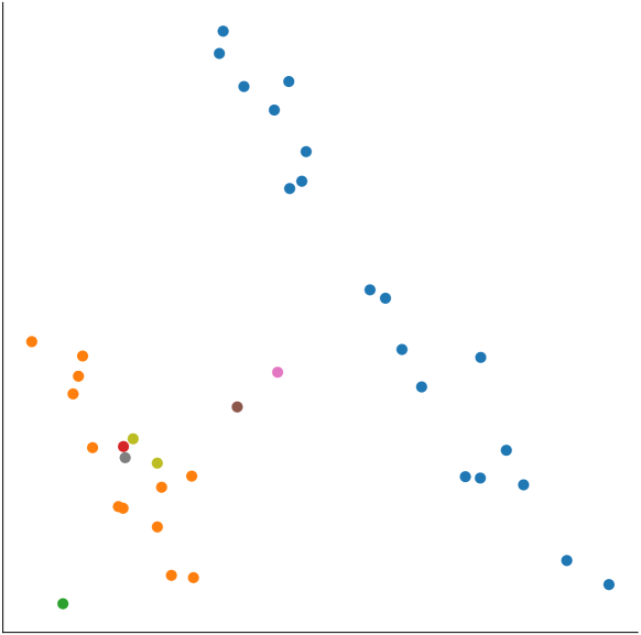
(b) $2$D projection.

Figure 6: PCA projections of the domain-specific variate embeddings learned during pre-training. OTiS unifies time series from diverse domains in a meaningful latent space, while correctly encoding the inter-variate relationships within a domain. Mono ($\bullet$) and stereo ($\bullet$) audio-specific embeddings cluster closely together, as do those for banking ($\bullet$) and economics ($\bullet$). Clear separation is observed for EEG-specific embeddings ($\bullet$), while also ECG-specific embeddings ($\bullet$) form a tight cluster.

E.2 Intra-Domain Analysis

A visualisation of the domain-specific variate embeddings for EEG and ECG are given in Figure 7 and Figure 8, respectively. We find that OTiS preserves low-level semantics specific to each domain, accurately capturing the relationships between variates.

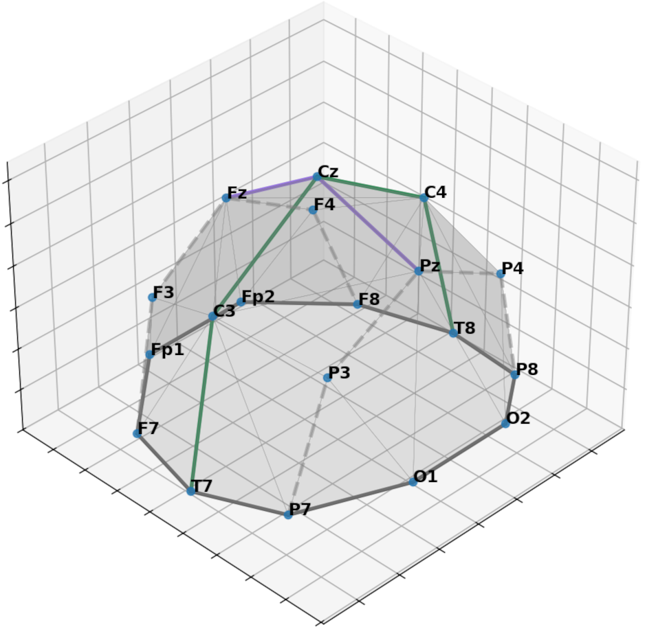
(a) True electrode layout.

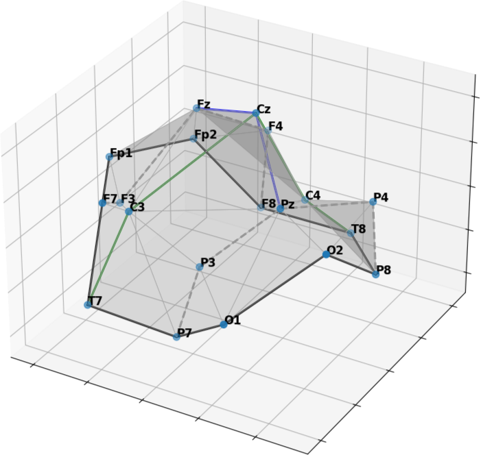
(b) Implicitly learned electrode layout.

Figure 7: $3$D PCA projections of the variate embeddings for $10$-$20$ system EEG recordings with $19$ electrodes learned during pre-training. The labels of each node correspond to the electrode names.

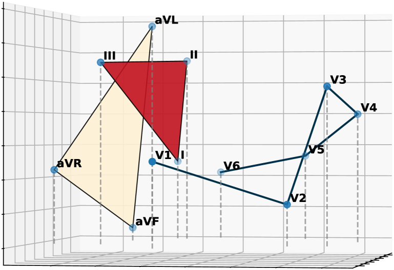
(a) Side view.

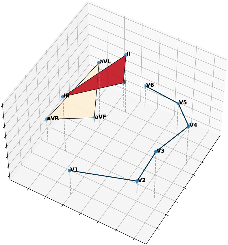
(b) Bird’s-eye view.

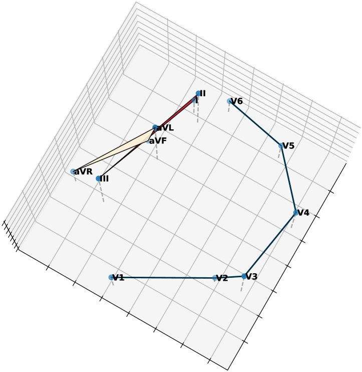
(c) Top view.

Figure 8: $3$D PCA projections of the variate embeddings for standard $12$-lead ECG learned during pre-training. The embeddings accurately reflect the true physiological structure of the ECG leads. The V$1$-V$6$ leads, arranged on the rib cage from the sternum to the mid-axillary line, represent a $3$D view of the human heart. In contrast, the I-II-III leads and aVR-aVL-aVF leads, derived from electrodes placed on one foot and both arms, form a planar $2$D triangle.

Appendix F Forecast Visualisation

We visualise the performance of our model on $6$ forecasting benchmarks in Figure 9.

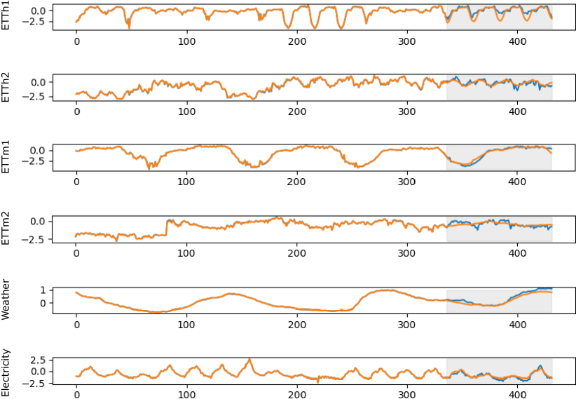
Figure 9: Visualisation of OTiS-Base forecast predictions on $6$ benchmark datasets. A forecasting horizon of $96$ time points is predicted from the past $336$ time points. Ground truth in blue, prediction in orange. Areas highlighted in grey are not visible to the model.

References

- Alabdulmohsin et al. (2022) Ibrahim Alabdulmohsin, Behnam Neyshabur, and Xiaohua Zhai. Revisiting neural scaling laws in language and vision. In Advances in Neural Information Processing Systems, 2022.
- Andrzejak et al. (2001) Ralph G Andrzejak, Klaus Lehnertz, Florian Mormann, Christoph Rieke, Peter David, and Christian E Elger. Indications of nonlinear deterministic and finite-dimensional structures in time series of brain electrical activity: Dependence on recording region and brain state. Physical Review E, 2001.
- Babayan et al. (2019) Anahit Babayan, Miray Erbey, Deniz Kumral, Janis D Reinelt, Andrea MF Reiter, Josefin Röbbig, H Lina Schaare, Marie Uhlig, Alfred Anwander, Pierre-Louis Bazin, et al. A mind-brain-body dataset of mri, eeg, cognition, emotion, and peripheral physiology in young and old adults. Scientific data, 2019.
- Bai et al. (2020) Wenjia Bai, Hideaki Suzuki, Jian Huang, Catherine Francis, Shuo Wang, Giacomo Tarroni, Florian Guitton, Nay Aung, Kenneth Fung, Steffen E Petersen, et al. A population-based phenome-wide association study of cardiac and aortic structure and function. Nature Medicine, 2020.
- Cherti et al. (2023) Mehdi Cherti, Romain Beaumont, Ross Wightman, Mitchell Wortsman, Gabriel Ilharco, Cade Gordon, Christoph Schuhmann, Ludwig Schmidt, and Jenia Jitsev. Reproducible scaling laws for contrastive language-image learning. In IEEE/CVF Conference on Computer Vision and Pattern Recognition, 2023.
- Chowdhery et al. (2023) Aakanksha Chowdhery, Sharan Narang, Jacob Devlin, Maarten Bosma, Gaurav Mishra, Adam Roberts, Paul Barham, Hyung Won Chung, Charles Sutton, Sebastian Gehrmann, et al. Palm: Scaling language modeling with pathways. Journal of Machine Learning Research, 2023.
- Das et al. (2024) Abhimanyu Das, Weihao Kong, Rajat Sen, and Yichen Zhou. A decoder-only foundation model for time-series forecasting. In International Conference on Machine Learning, 2024.
- Dong et al. (2024) Jiaxiang Dong, Haixu Wu, Haoran Zhang, Li Zhang, Jianmin Wang, and Mingsheng Long. Simmtm: A simple pre-training framework for masked time-series modeling. In Advances in Neural Information Processing Systems, 2024.
- Dosovitskiy et al. (2021) Alexey Dosovitskiy, Lucas Beyer, Alexander Kolesnikov, Dirk Weissenborn, Xiaohua Zhai, Thomas Unterthiner, Mostafa Dehghani, Matthias Minderer, Georg Heigold, Sylvain Gelly, Jakob Uszkoreit, and Neil Houlsby. An image is worth 16x16 words: Transformers for image recognition at scale. In International Conference on Learning Representations, 2021.
- Fawaz et al. (2018) Hassan Ismail Fawaz, Germain Forestier, Jonathan Weber, Lhassane Idoumghar, and Pierre-Alain Muller. Transfer learning for time series classification. In IEEE International Conference on Big Data. IEEE, 2018.
- Gasparin et al. (2022) Alberto Gasparin, Slobodan Lukovic, and Cesare Alippi. Deep learning for time series forecasting: The electric load case. CAAI Transactions on Intelligence Technology, 2022.
- Geirhos et al. (2019) Robert Geirhos, Patricia Rubisch, Claudio Michaelis, Matthias Bethge, Felix A Wichmann, and Wieland Brendel. Imagenet-trained cnns are biased towards texture; increasing shape bias improves accuracy and robustness. International Conference on Learning Representations, 2019.
- Gemmeke et al. (2017) Jort F Gemmeke, Daniel PW Ellis, Dylan Freedman, Aren Jansen, Wade Lawrence, R Channing Moore, Manoj Plakal, and Marvin Ritter. Audio set: An ontology and human-labeled dataset for audio events. In IEEE International Conference on Acoustics, Speech and Signal Processing (ICASSP), 2017.
- Gordon et al. (2021) Mitchell A Gordon, Kevin Duh, and Jared Kaplan. Data and parameter scaling laws for neural machine translation. In Conference on Empirical Methods in Natural Language Processing, 2021.
- Goswami et al. (2024) Mononito Goswami, Konrad Szafer, Arjun Choudhry, Yifu Cai, Shuo Li, and Artur Dubrawski. Moment: A family of open time-series foundation models. International Conference on Machine Learning, 2024.
- Gow et al. (2023) Brian Gow, Tom Pollard, Larry A Nathanson, Alistair Johnson, Benjamin Moody, Chrystinne Fernandes, Nathaniel Greenbaum, Seth Berkowitz, Dana Moukheiber, Parastou Eslami, et al. Mimic-iv-ecg-diagnostic electrocardiogram matched subset. PyhsioNet, 2023.
- Gupta et al. (2020) Priyanka Gupta, Pankaj Malhotra, Jyoti Narwariya, Lovekesh Vig, and Gautam Shroff. Transfer learning for clinical time series analysis using deep neural networks. Journal of Healthcare Informatics Research, 4(2):112–137, 2020.
- He et al. (2022) Kaiming He, Xinlei Chen, Saining Xie, Yanghao Li, Piotr Dollár, and Ross Girshick. Masked autoencoders are scalable vision learners. In IEEE/CVF Conference on Computer Vision and Pattern Recognition, 2022.
- Ismail Fawaz et al. (2019) Hassan Ismail Fawaz, Germain Forestier, Jonathan Weber, Lhassane Idoumghar, and Pierre-Alain Muller. Deep learning for time series classification: a review. Data Mining and Knowledge Discovery, 2019.
- Iwana & Uchida (2021) Brian Kenji Iwana and Seiichi Uchida. An empirical survey of data augmentation for time series classification with neural networks. Plos one, 16(7):e0254841, 2021.
- Jiang et al. (2024) Weibang Jiang, Liming Zhao, and Bao liang Lu. Large brain model for learning generic representations with tremendous EEG data in BCI. In International Conference on Learning Representations, 2024.
- Jin et al. (2023) Ming Jin, Shiyu Wang, Lintao Ma, Zhixuan Chu, James Y Zhang, Xiaoming Shi, Pin-Yu Chen, Yuxuan Liang, Yuan-Fang Li, Shirui Pan, et al. Time-llm: Time series forecasting by reprogramming large language models. International Conference on Learning Representations, 2023.
- Jurcak et al. (2007) Valer Jurcak, Daisuke Tsuzuki, and Ippeita Dan. 10/20, 10/10, and 10/5 systems revisited: their validity as relative head-surface-based positioning systems. Neuroimage, 34(4):1600–1611, 2007.
- Kaplan et al. (2020) Jared Kaplan, Sam McCandlish, Tom Henighan, Tom B Brown, Benjamin Chess, Rewon Child, Scott Gray, Alec Radford, Jeffrey Wu, and Dario Amodei. Scaling laws for neural language models. arXiv preprint arXiv:2001.08361, 2020.
- Kreuzer et al. (2021) Devin Kreuzer, Dominique Beaini, Will Hamilton, Vincent Létourneau, and Prudencio Tossou. Rethinking graph transformers with spectral attention. Advances in Neural Information Processing Systems, 2021.
- Lai et al. (2018) Guokun Lai, Wei-Cheng Chang, Yiming Yang, and Hanxiao Liu. Modeling long-and short-term temporal patterns with deep neural networks. In International ACM SIGIR conference on research & development in information retrieval, 2018.
- Lessmeier et al. (2016) Christian Lessmeier, James Kuria Kimotho, Detmar Zimmer, and Walter Sextro. Condition monitoring of bearing damage in electromechanical drive systems by using motor current signals of electric motors: A benchmark data set for data-driven classification. In PHM Society European Conference, 2016.
- Li et al. (2023) Zhe Li, Zhongwen Rao, Lujia Pan, Pengyun Wang, and Zenglin Xu. Ti-mae: Self-supervised masked time series autoencoders. arXiv preprint arXiv:2301.08871, 2023.
- Liu et al. (2009) Jiayang Liu, Lin Zhong, Jehan Wickramasuriya, and Venu Vasudevan. uwave: Accelerometer-based personalized gesture recognition and its applications. Pervasive and Mobile Computing, 2009.
- Liu et al. (2024) Yong Liu, Haoran Zhang, Chenyu Li, Xiangdong Huang, Jianmin Wang, and Mingsheng Long. Timer: Generative pre-trained transformers are large time series models. International Conference on Machine Learning, 2024.
- McCracken & Ng (2016) Michael W McCracken and Serena Ng. Fred-md: A monthly database for macroeconomic research. Journal of Business & Economic Statistics, 2016.
- Nie et al. (2023) Yuqi Nie, Nam H Nguyen, Phanwadee Sinthong, and Jayant Kalagnanam. A time series is worth 64 words: Long-term forecasting with transformers. In International Conference on Learning Representations, 2023.
- Oquab et al. (2024) Maxime Oquab, Timothée Darcet, Théo Moutakanni, Huy V. Vo, Marc Szafraniec, Vasil Khalidov, Pierre Fernandez, Daniel HAZIZA, Francisco Massa, Alaaeldin El-Nouby, Mido Assran, Nicolas Ballas, Wojciech Galuba, Russell Howes, Po-Yao Huang, Shang-Wen Li, Ishan Misra, Michael Rabbat, Vasu Sharma, Gabriel Synnaeve, Hu Xu, Herve Jegou, Julien Mairal, Patrick Labatut, Armand Joulin, and Piotr Bojanowski. DINOv2: Learning robust visual features without supervision. Transactions on Machine Learning Research, 2024.
- Oreshkin et al. (2019) Boris N Oreshkin, Dmitri Carpov, Nicolas Chapados, and Yoshua Bengio. N-beats: Neural basis expansion analysis for interpretable time series forecasting. International Conference on Learning Representations, 2019.
- PhysioBank (2000) PhysioToolkit PhysioBank. Physionet: components of a new research resource for complex physiologic signals. Circulation, 2000.
- Pirkis et al. (2021) Jane Pirkis, Ann John, Sangsoo Shin, Marcos DelPozo-Banos, Vikas Arya, Pablo Analuisa-Aguilar, Louis Appleby, Ella Arensman, Jason Bantjes, Anna Baran, et al. Suicide trends in the early months of the covid-19 pandemic: an interrupted time-series analysis of preliminary data from 21 countries. The Lancet Psychiatry, 2021.
- Radford et al. (2018) Alec Radford, Karthik Narasimhan, Tim Salimans, Ilya Sutskever, et al. Improving language understanding by generative pre-training. OpenAI, 2018.
- Radhakrishnan et al. (2023) Adityanarayanan Radhakrishnan, Sam F Friedman, Shaan Khurshid, Kenney Ng, Puneet Batra, Steven A Lubitz, Anthony A Philippakis, and Caroline Uhler. Cross-modal autoencoder framework learns holistic representations of cardiovascular state. Nature Communications, 2023.
- Ravi et al. (2024) Nikhila Ravi, Valentin Gabeur, Yuan-Ting Hu, Ronghang Hu, Chaitanya Ryali, Tengyu Ma, Haitham Khedr, Roman Rädle, Chloe Rolland, Laura Gustafson, et al. Sam 2: Segment anything in images and videos. arXiv preprint arXiv:2408.00714, 2024.
- Ravuri et al. (2021) Suman Ravuri, Karel Lenc, Matthew Willson, Dmitry Kangin, Remi Lam, Piotr Mirowski, Megan Fitzsimons, Maria Athanassiadou, Sheleem Kashem, Sam Madge, et al. Skilful precipitation nowcasting using deep generative models of radar. Nature, 2021.
- Schoffelen & Gross (2009) Jan-Mathijs Schoffelen and Joachim Gross. Source connectivity analysis with meg and eeg. Human brain mapping, 30(6):1857–1865, 2009.
- Sezer et al. (2020) Omer Berat Sezer, Mehmet Ugur Gudelek, and Ahmet Murat Ozbayoglu. Financial time series forecasting with deep learning: A systematic literature review: 2005–2019. Applied Soft Computing, 2020.
- Sudlow et al. (2015) Cathie Sudlow, John Gallacher, Naomi Allen, Valerie Beral, Paul Burton, John Danesh, Paul Downey, Paul Elliott, Jane Green, Martin Landray, Bette Liu, Paul Matthews, Giok Ong, Jill Pell, Alan Silman, Alan Young, Tim Sprosen, Tim Peakman, and Rory Collins. UK biobank: an open access resource for identifying the causes of a wide range of complex diseases of middle and old age. PLoS Medicine, 2015.
- Taieb et al. (2012) Souhaib Ben Taieb, Gianluca Bontempi, Amir F Atiya, and Antti Sorjamaa. A review and comparison of strategies for multi-step ahead time series forecasting based on the nn5 forecasting competition. Expert Systems with Applications, 2012.
- Tang et al. (2020) Chi Ian Tang, Ignacio Perez-Pozuelo, Dimitris Spathis, and Cecilia Mascolo. Exploring contrastive learning in human activity recognition for healthcare. arXiv preprint arXiv:2011.11542, 2020.
- Touvron et al. (2023) Hugo Touvron, Thibaut Lavril, Gautier Izacard, Xavier Martinet, Marie-Anne Lachaux, Timothée Lacroix, Baptiste Rozière, Naman Goyal, Eric Hambro, Faisal Azhar, et al. Llama: Open and efficient foundation language models. arXiv preprint arXiv:2302.13971, 2023.
- Turgut et al. (2023) Özgün Turgut, Philip Müller, Paul Hager, Suprosanna Shit, Sophie Starck, Martin J Menten, Eimo Martens, and Daniel Rueckert. Unlocking the diagnostic potential of electrocardiograms through knowledge transfer from cardiac magnetic resonance imaging. arXiv preprint arXiv:2308.05764, 2023.
- UCI (2024) UCI. Uci electricity load time series dataset. UCI, 2024. https://archive.ics.uci.edu/dataset/321/electricityloaddiagrams20112014.
- Van Dijk et al. (2022) Hanneke Van Dijk, Guido Van Wingen, Damiaan Denys, Sebastian Olbrich, Rosalinde Van Ruth, and Martijn Arns. The two decades brainclinics research archive for insights in neurophysiology (tdbrain) database. Scientific data, 2022.
- Vaswani et al. (2017) Ashish Vaswani, Noam Shazeer, Niki Parmar, Jakob Uszkoreit, Llion Jones, Aidan N Gomez, Łukasz Kaiser, and Illia Polosukhin. Attention is all you need. Advances in Neural Information Processing Systems, 30, 2017.
- Wetterdienst (2024) Deutscher Wetterdienst. Temperature dataset. DWD, 2024. https://www.dwd.de/DE/leistungen/klimadatendeutschland/klarchivtagmonat.html.
- Wetterstation (2024) Wetterstation. Weather dataset. Wetter, 2024. https://www.bgc-jena.mpg.de/wetter/.
- Wickstrøm et al. (2022) Kristoffer Wickstrøm, Michael Kampffmeyer, Karl Øyvind Mikalsen, and Robert Jenssen. Mixing up contrastive learning: Self-supervised representation learning for time series. Pattern Recognition Letters, 2022.
- Woo et al. (2022) Gerald Woo, Chenghao Liu, Doyen Sahoo, Akshat Kumar, and Steven Hoi. CoST: Contrastive learning of disentangled seasonal-trend representations for time series forecasting. In International Conference on Learning Representations, 2022.
- Woo et al. (2024) Gerald Woo, Chenghao Liu, Akshat Kumar, Caiming Xiong, Silvio Savarese, and Doyen Sahoo. Unified training of universal time series forecasting transformers. International Conference on Machine Learning, 2024.
- Wu et al. (2021) Haixu Wu, Jiehui Xu, Jianmin Wang, and Mingsheng Long. Autoformer: Decomposition transformers with auto-correlation for long-term series forecasting. In Advances in Neural Information Processing Systems, 2021.
- Wu et al. (2022a) Haixu Wu, Tengge Hu, Yong Liu, Hang Zhou, Jianmin Wang, and Mingsheng Long. Timesnet: Temporal 2d-variation modeling for general time series analysis. In International Conference on Learning Representations, 2022a.
- Wu et al. (2022b) Xun Wu, Wei-Long Zheng, Ziyi Li, and Bao-Liang Lu. Investigating eeg-based functional connectivity patterns for multimodal emotion recognition. Journal of neural engineering, 19(1):016012, 2022b.
- Yang et al. (2024) Chaoqi Yang, M Westover, and Jimeng Sun. Biot: Biosignal transformer for cross-data learning in the wild. Advances in Neural Information Processing Systems, 2024.
- Ye & Dai (2021) Rui Ye and Qun Dai. Implementing transfer learning across different datasets for time series forecasting. Pattern Recognition, 2021.
- Yue et al. (2022) Zhihan Yue, Yujing Wang, Juanyong Duan, Tianmeng Yang, Congrui Huang, Yunhai Tong, and Bixiong Xu. Ts2vec: Towards universal representation of time series. In AAAI Conference on Artificial Intelligence, 2022.
- Zeng et al. (2023) Ailing Zeng, Muxi Chen, Lei Zhang, and Qiang Xu. Are transformers effective for time series forecasting? In AAAI Conference on Artificial Intelligence, 2023.
- Zhang et al. (2022) Xiang Zhang, Ziyuan Zhao, Theodoros Tsiligkaridis, and Marinka Zitnik. Self-supervised contrastive pre-training for time series via time-frequency consistency. Advances in Neural Information Processing Systems, 2022.
- Zhang et al. (2010) Zhi-Min Zhang, Shan Chen, and Yi-Zeng Liang. Baseline correction using adaptive iteratively reweighted penalized least squares. Analyst, 2010.
- Zheng & Lu (2015) Wei-Long Zheng and Bao-Liang Lu. Investigating critical frequency bands and channels for EEG-based emotion recognition with deep neural networks. IEEE Transactions on Autonomous Mental Development, 2015.
- Zhou et al. (2021) Haoyi Zhou, Shanghang Zhang, Jieqi Peng, Shuai Zhang, Jianxin Li, Hui Xiong, and Wancai Zhang. Informer: Beyond efficient transformer for long sequence time-series forecasting. In AAAI Conference on Artificial Intelligence, 2021.
- Zhou et al. (2022) Jinghao Zhou, Chen Wei, Huiyu Wang, Wei Shen, Cihang Xie, Alan Yuille, and Tao Kong. Image BERT pre-training with online tokenizer. In International Conference on Learning Representations, 2022.
- Zhou et al. (2023) Tian Zhou, Peisong Niu, Liang Sun, Rong Jin, et al. One fits all: Power general time series analysis by pretrained lm. Advances in neural information processing systems, 2023.