Feature-centric nonlinear autoregressive models
Abstract
We propose a novel feature-centric approach to surrogate modeling of dynamical systems driven by time-varying exogenous excitations. This approach, named Functional Nonlinear AutoRegressive with eXogenous inputs (-NARX), aims to approximate the system response based on temporal features of both the exogenous inputs and the system response, rather than on their values at specific time lags. This is a major step away from the discrete-time-centric approach of classical NARX models, which attempts to determine the relationship between selected time steps of the input/output time series. By modeling the system in a time-feature space instead of the original time axis, -NARX can provide more stable long-term predictions and drastically reduce the reliance of the model performance on the time discretization of the problem.
-NARX, like NARX, acts as a framework and is not tied to a single implementation. In this work, we introduce an -NARX implementation based on principal component analysis and polynomial basis functions. To further improve prediction accuracy and computational efficiency, we also introduce a strategy to identify and fit a sparse model structure, thanks to a modified hybrid least angle regression approach that minimizes the expected forecast error, rather than the one-step-ahead prediction error.
Since -NARX is particularly well-suited to modeling engineering structures typically governed by physical processes, we investigate the behavior and capabilities of our -NARX implementation on two case studies: an eight-story building under wind loading and a three-story steel frame under seismic loading. While the first case study highlights the simple and intuitive parametrization of the presented -NARX implementation, the second case study demonstrates its high accuracy and prediction stability in more complex nonlinear problems.
Our results demonstrate that -NARX has several favorable properties over classical NARX, making it well suited to emulate engineering systems with high accuracy over extended time periods.
1 Introduction
Many real-world problems are inherently time-dependent, with systems continuously evolving under the influence of external factors and excitations. Accurate modeling of these dynamical systems is essential in numerous engineering disciplines, be it for system control Levin and Narendra (1996); Hu et al. (2024), maintenance planning Langeron et al. (2021); Samsuri et al. (2023), fault detection and diagnosis Mattson and Pandit (2006); Gao et al. (2016), design assessment and optimization Yu et al. (2023); Deshmukh and Allison (2017) or uncertainty quantification Mai et al. (2016); Bhattacharyya et al. (2020) and reliability analysis Garg et al. (2022); Zhou and Li (2023); Zhang et al. (2024).
Although these applications are different in nature, they are similar in that they often require to learn the dependence between the time-varying external factors or actions and the corresponding system response. This dependence is typically modeled by so-called autoregressive models with exogenous inputs (ARX). By using the exogenous inputs in conjunction with their own past predictions, these models are powerful predictors for dynamical systems, especially when used in their nonlinear variant, known as NARX Billings (2013). NARX models have been successfully applied to many engineering structures and components, such as mooring lines Yetkin et al. (2017); Zhang et al. (2024), gas or wind turbines Chiras et al. (2001); Schlechtingen and Ferreira Santos (2011), multi-story buildings Spiridonakos and Chatzi (2015); Li et al. (2021), marine structures Kim (2015); Ramin et al. (2023) or geotechnical structures Wunsch et al. (2018); Dassanayake et al. (2023).
This success is partially due to their versatility, which allows one to combine them with powerful techniques from the fields of surrogate modeling and machine learning, such as Gaussian process modeling Murray-Smith et al. (1999); Kocijan (2012); Koziel et al. (2014); Worden et al. (2018), support vector regression Acuña et al. (2012); Ranković et al. (2014); Zhang et al. (2017), neural networks Siegelmann et al. (1997); Li et al. (2021); Song et al. (2022) or a wide array of basis functions Aguirre and Billings (1993); Coca and Billings (2001); Chen et al. (2008). They have also been successfully deployed in applications with categorical outcomes by combining them with logistic regression Ayala et al. (2017); Lacerda Junior et al. (2021).
Fitting a predictive model to existing data is generally a difficult task, and since NARX models rely on the time discretization of the problem at hand, they pose one additional key challenge: the selection of lags to be considered. In other words, how to select which time instants of the exogenous and autoregressive inputs are to be considered in the model? This selection has to be made from a possibly large set of candidate lags, for example, if the time-discretization of the problem is small or the model’s memory long. While no universal solution to this problem is currently available from the relevant literature, several ways to directly select important lags, or at least decimate the candidate lags, have been proposed. Examples include trial-and-error-based approaches Chen and Ni (2011); Schär et al. (2024); Awtoniuk et al. (2019) or correlation-based approaches Wei and Billings (2008); Cheng et al. (2011). An approach named “clustering” has been proposed by Aguirre and Billings (1995); Aguirre and Jácome (1998) for the specific case of polynomial NARX models. For the special class of linear-in-the-parameters problems Billings (2013), dedicated sparse solvers have also been employed to better handle a large number of regressors Spinelli et al. (2006); Billings (2013); Falsone et al. (2014); Yuzhu Guo and Wei (2015); Mai et al. (2016); F. Bianchi and Piroddi (2017); Li et al. (2021).
NARX models are most often trained by minimizing the one-step-ahead prediction (OSA) error, as this is very fast and sometimes even a closed-form solution exists. However, minimization of OSA errors can lead to poor results when the trained model is used in a forecast setup Piroddi (2008). In extreme cases, the model predictions can even diverge over time Piroddi (2008); Farina and Piroddi (2009); Yu et al. (2023). Therefore, dedicated solvers have been developed to minimize the forecast error. For instance, Piroddi and Spinelli (2003); Piroddi (2008); Piroddi et al. (2010) present pruning-based methods, while Farina and Piroddi (2009, 2010) introduced gradient-based algorithms. The main disadvantage of these approaches is the heavily increased computational costs compared to the minimization of the OSA error.
Several works Aguirre (1994); Billings and Aguirre (1995); Spinelli et al. (2006) argue that the negative consequences of an OSA error minimization are more likely to happen if the sampling frequency of the problem is high. The reason lies in the high temporal correlation between adjacent time steps, which in turn can lead to the over-reliance on the first autoregressive lag, resulting in drastic losses in terms of the final model performance Piroddi and Spinelli (2003).
Interestingly, all these limitations are related to the discretization of the time axis, in conjunction with the exclusive focus of classical ARX modeling on individual discrete time step values, a characteristic we refer to as a discrete-time view on ARX modeling. Although many methods have been developed to mitigate these problems, they remain fully committed to this discrete-time view. This raises the question of whether alternative views can offer advantages over the discrete-time one.
In this work, we revisit the fundamentals of autoregressive problems with exogenous inputs. We propose and discuss an alternative continuous functional view, demonstrating how it can address the problem of lag selection, while at the same time mitigating the problem of over-reliance, thus improving forecast stability and accuracy. This continuous functional approach leverages the temporal correlation and smoothness exhibited by many time-dependent processes, especially in physical systems or structural responses. Due to its underlying principles, we refer to this approach as functional nonlinear autoregressive with exogenous inputs (-NARX) modeling. The way -NARX modeling uses temporal features of the input and output signals allows the problem to still be posed as a linear regression problem, and therefore -NARX remains compatible with most algorithms developed for classical NARX modeling. The use of temporal features can also result in sparser representations of both the input and output signals, and promotes independence between regressors, which can in turn be exploited through compressed sensing algorithms Eldar and Kutyniok (2012), and thus create small models with high expressiveness.
This paper is structured as follows: we begin with the description of the -NARX approach in the Sections 2 and 3. This includes a brief recap on the basics of NARX modeling, followed by its extension to -NARX, as well as a concrete implementation of an -NARX model using a combination of principal-component analysis and a polynomial regression model. In Section 4, we present two case studies to investigate the behavior and properties of the presented -NARX implementation and demonstrate its performance on a complex dynamical system. A discussion on the -NARX approach and the presented results, as well as concluding remarks, are given in Section 5.
2 Methodology
2.1 Autoregressive modeling with exogenous inputs
Consider a deterministic dynamical system evolving along the time axis . The system is excited by a (possibly high-dimensional) time-varying exogenous input . Given a vector of initial conditions , the system response at any time instant is denoted as:
| (1) |
Here, the notation indicates that the system response at time depends on the excitation up to and including time . To simplify the notation, we will subsequently omit unless it is strictly necessary.
Suppose we want to construct a dynamic surrogate model that approximates the response of the system such that:
| (2) |
In this work, we focus in particular on dynamic surrogates based on nonlinear autoregressive models with exogenous inputs (NARX). At the core of a NARX model lies the idea that the system’s dynamics can be captured at a set of discrete time steps and that the system response at a time step in the near future can be predicted as a function of past and current exogenous inputs, as well as past outputs:
| (3) |
where is a residual term with zero mean and standard deviation . Let us assume the mapping function is parametric, and that it can be characterized by a finite set of parameters . Then the process of training (or fitting) a NARX model consists in estimating the values of from a set of system input/output discretized trajectories . We refer to each such pair as a realization or observation of the system, while the full set of realizations is called the experimental design (ED):
| (4) |
The number of realizations in the experimental design is usually relatively small (), since the acquisition of even a single observation may require an expensive experiment or simulation.
We can make the notation more explicit by rewriting Eq. (3) as:
| (5) |
where the vector reads:
| (6) |
We refer to the delayed values as the autoregressive lags and to as the exogenous input lags, where is a non-negative integer value to preserve the causality of the original system. The integers are typically referred to as the model orders.
By stacking the vectors for all time steps, we obtain the so-called design matrix , where and where due to the use of lagged values. Similarly, we stack the values to obtain the corresponding output vector :
| (7) |
with .
Note that despite considering time-dependent data, the sample pairs no longer need to follow a temporal ordering. Consequently, the matrices and vectors , with , from different realizations within the experimental design can be concatenated to form a larger matrix and vector :
| (8) |
We now recall from Eq. (3), that the objective is to develop a predictive model , characterized by its parameters , using only a limited set of observations . The estimation of these model parameters can then be performed by minimizing a suitable loss function that represents the discrepancy between the experimental design observations and the model predictions:
| (9) |
Common choices for include polynomials, for which represents the coefficient vector Aguirre and Billings (1993), neural networks, with denoting the corresponding weights and biases Siegelmann et al. (1997), among others. A class of models frequently adopted in the literature is that of linear-in-the-parameters models Billings (2013). This class is particularly attractive, because it allows the optimization problem in Eq. (9) to be solved using least-squares minimization:
| (10) |
where denotes a possibly nonlinear mapping between lags and regressors, e. g. multivariate polynomials. By defining the coefficient vector can therefore be computed analytically using ordinary least squares (OLS):
| (11) |
Although OLS is a viable option to solve for , more advanced regularized regression techniques are often used to promote a sparse set of coefficients, resulting in a more stable model with improved generalization capabilities. A prominent example is given by LASSO (least absolute shrinkage and selection operator) regression Tibshirani (1996) which promotes sparsity introducing an penalty term with regularization parameter for the estimation of the coefficient vector:
| (12) |
Among the available solvers of the LASSO problem, least angle regression (LARS, Efron et al. (2004)) has been proven particularly effective in the context of polynomial regression (Blatman and Sudret, 2011), and is the technique of choice in this work (see Section 3.3).
A detailed explanation and discussion on polynomial NARX models, as a concrete implementation of a linear-in-the-parameters model, and their synergy with sparse regression techniques will be provided in Sections 3.2 and 3.3.
Considering again the linear-in-the-parameters model with its mapping and coefficient set , we can calculate the so-called one-step-ahead (OSA) prediction on a new input vector as:
| (13) |
Note, however, that in order to construct , we require the true model output up to time (see Eq. (6)). While many applications of autoregressive modeling are focused on one-step-ahead predictions, in surrogate modeling this is typically not the case. With a surrogate model, we aim to approximate the true model response throughout the duration of the external dynamic loading, i. e. the whole trajectory. We refer to this as model forecast, or simply as model prediction. The model forecast is based on iteratively evaluating one-step-ahead predictions, and using the corresponding approximate response as the autoregressive input for the next step, resulting in:
| (14) |
which contains the previous predictions . In order to perform this prediction, the model needs to be initialized with values that match the initial conditions of the system under investigation. This is done by setting the initial values of the system response to appropriate values. The surrogate prediction can be initialized to zero Worden and Barthorpe (2012) or other sensible values Schär et al. (2024), depending on the specific application.
2.2 Limitations of classical ARX modeling
If a nonlinear ARX (NARX) model is fitted as described in Eq. (9) or (10), the associated regression problem becomes intractable if the number of exogenous inputs or the model orders are large. This is due to the highly non-linear scaling of the number of regressors with the problem dimension, a phenomenon known as the curse of dimensionality Verleysen and François (2005). To handle systems requiring large model orders, while still keeping the dimensionality of manageable, Schär et al. (2024) introduced the use of a non-evenly spaced set of lags, determined through trial and error on the available training data. Although it was shown to be a viable option in terms of the accuracy of the final model, trial and error can be time consuming and does not provide a good guarantee of near-optimal performance. Alternatively, Awtoniuk et al. (2019) proposed to select a subset of the lags following certain pre-determined patterns, for example only odd or even lags. However, this approach is limited because regularly spaced lags can cause loss of important information or aliasing effects if significant decimation is performed.
An approach limited to linear-in-the-parameters models, as described in Eq. (10), involves the use of sparse regression solvers. In particular, several forward selection algorithms have gained popularity Billings (2013); Yuzhu Guo and Wei (2015); Mai et al. (2016). Unfortunately, these sparse solvers also have practical limitations regarding the number of regressors. With a very large number of regressors, efficiency decreases, and computational costs or hardware resources can become a bottleneck.
A more specific method, called term clustering, was developed for polynomial NARX models to discard entire clusters of lagged values belonging to irrelevant nonlinearities Aguirre and Billings (1995); Aguirre and Jácome (1998); Pulecchi and Piroddi (2007). Selecting the correct clusters can also be particularly challenging, especially in the presence of noise. The specificity to a certain class of NARX models may also have hindered the widespread adoption of this method.
Another difficulty arises when fitting ARX models in a regression setting when the time increment is small, e. g. due to requirements of the numerical solver of choice. Very small can lead to numerical instability during the regression task, due to high correlation between lags. In Piroddi and Spinelli (2003) it is shown how a very high sampling rate can also lead to an overestimation of the importance of the most recent autoregressive lag. This over-reliance can have a detrimental effect on the model forecast. Unfortunately, data decimation to alleviate these issues is not always viable, since the data may be correctly sampled for signal reconstruction purposes and may only appear oversampled with respect to the prediction problem Piroddi and Spinelli (2003); Lataniotis et al. (2020).
We observe that a common cause of all these limitations lies in the explicitly discrete-time-centric nature of classical autoregressive modeling, which assumes a specific time axis discretization, rather than the intrinsically continuous nature of the response of dynamical systems to exogenous excitations. In the following sections, we therefore propose and discuss a novel continuous-functional view of the ARX methodology, which tackles autoregressive problems from a continuous perspective and discretizes the problem only in a final stage for numerical purposes.
2.3 Moving from a discrete time to a continuous functional view of autoregressive modeling
Real-world processes are inherently continuous in time, and the discretization of the time axis is merely a tool required by digital data storage or numerical simulators. This fact is acknowledged, for example, by continuous-time system identification, which treats the dynamics of the system as a differential equation Billings (2013). Interestingly, NARX models also find their application in this area. They are used as intermediate discrete parametric models, which are then used to derive continuous-time models. Yet again, the focus lies on the fact that the problem can be discretized in time and the NARX models do not fully exploit the continuous nature of the underlying process.
To devise a less discrete view of ARX modeling, let us first consider a continuous-time signal , as depicted in Figure 1. We set our focus on the signal during a time window , indexed by a time , with endpoint and finite length , i. e., we define the continuous interval , such that:
| (15) |
We assume that the signal exhibits some form of temporal regularity, and that its dynamic information can be represented by a set of continuous temporal features , e. g. cosine functions, wavelets, polynomials, etc., of the form:
| (16) |
where the represent the projection of the original function in the time window onto the -th continuous temporal feature . An interesting property of the right-hand side of Eq. (16) is that it explicitly decomposes the time dependence of the underlying function in two different components: the scalar coefficients encoding the “global” time , but not the “local” time within the window, while the continuous features encode the dependence on instead. In other words, we decompose a moving window of duration , starting from the global time , on a set of temporal features .
For illustrative purposes, the bottom plot in Figure 1 illustrates such a finite set of continuous features weighted by their coefficients , such that the response of the function on the highlighted time window is decomposed as:
| (17) |
Representing a time-dependent signal through its properties within a fixed-width moving window is a well-established technique in signal processing, widely known as the sliding window Bastiaans (1985); Badeau et al. (2004). Nevertheless, to the authors’ best knowledge, this is the first time this approach is combined within an autoregressive setting. Popular choices to represent time-dependent signals in the form of Eq. (16) include Fourier transforms Bracewell (1989), and Karhunen-Loève expansions Loève (1955). An advantage of structured representations like these is that real-world processes are often represented adequately even using a heavily truncated set of features. This property is taken advantage of, for example, for dimensionality reduction Bengio et al. (2006) or lossy signal compression Strang and Nguyen (1996). Autoregressive inputs and responses often exhibit strong temporal regularity and predictable behavior, originating from the inert physical processes that govern them, and are therefore suitable for this type of representation. For physical systems, domain-specific knowledge may be even leveraged to produce particularly efficient representations.
In the context of autoregressive simulation, additional features may also be considered to simplify the construction of the input/output map in Eq. (3). These include classical statistics in the sliding window, such as moving averages, variances, dominating frequencies, principal components, singular value decomposition eigenmodes, among others. The usefulness of using prior knowledge about the physics of the system in the ARX modeling process has recently been demonstrated in Schär et al. (2024).
In the following section, we will discuss how we can use features of the exogenous inputs and output to reformulate the classical discrete-time view on ARX into a continuous functional view that can mitigate or even eliminate some of its limitations.
2.4 Functional nonlinear autoregressive with exogenous inputs modeling (-NARX)
We introduce here our adaptation of NARX modelling designed to work with features, rather than lags. We start by defining the time-dependent information vector , that gathers all exogenous inputs together with the model response within a time window as follows:
| (18) |
where is a small positive arbitrary time increment.
Intuitively, the window width can be considered as the memory of the model. Ideally, it is close to the effective memory of the system with respect to the corresponding variable. We define the effective memory as the look-back time such that the effect of the independent variable on the dependent variable in Eq. (3) becomes negligibly small. In principle, when considering complex systems with different processes and inputs, a different memory could be considered for each component of in Eq. (18), resulting in a set of memories . To simplify our notation and avoid adding complexity, we assume, without loss of generality, a uniform memory for all input and output components from this point onward. For each of the components in Eq. (18), we now introduce a corresponding function , which extracts a set of features :
| (19) |
No restrictions are made on the nature of the transforms , nor on the dimensionality of each feature-set . Different elements of the information vector can have different transforms, or different truncation schemes. For example, some exogenous input may exhibit a strong cyclic behavior, and the corresponding may represent a subset of its Fourier coefficients, while some other input, say , may instead have a smoother behavior, better described by a polynomial representation with coefficients .
We gather all the feature sets into a single feature vector , with :
| (20) |
Note that is the total number of relevant features extracted from the components. We can now adapt the classical NARX approach in Section 2.1, by capitalizing on the feature vector . The goal is to approximate a near future response value as a function of :
| (21) |
An interesting aspect of this formulation is that it does not make any assumption about the discretization of the time axis. This is because the features in Eq. (16)) are not directly dependent on the local time axis (see Figure 1), only the transform to extract them is. In other words, the specific discretization choices of the sliding time window only affect how the features are extracted (and therefore possibly the accuracy of their extraction), but not their interpretation or physical meaning. To give a concrete example, assume that the chosen features of a chosen continuous window can be exactly represented by a second order polynomial. The set of features is then given by the three polynomial coefficients such that:
| (22) |
If is then arbitrarily discretized on the time axis, the values of will remain unchanged. Nevertheless, their extraction accuracy from a discretized dataset may depend on the discretization itself. In the given example, at least three time samples would be needed to exactly determine the coefficient of a second degree polynomial interpolant. This natural robustness to oversampling is especially interesting in the context of surrogate modeling of numerical dynamical systems, where the sampling frequency of the solver is often many times higher than the actual frequency content of the modeled signal responses. It is also an important property for the mitigation of the over-reliance problem of classical NARX at high sampling rates (see Section 2.2).
Note that in Eq. (18) is essentially a continuous equivalent of in Eq. (6), and that we can write the time window in a discretized form as follows:
| (23) |
where . The key difference to the classical ARX modeling introduced in Section 2.1 lies in the use of the features generated through the functions , rather than in the original set of input/outputs , hence exploiting the smoothness and regularity of the process being modeled.
A direct advantage of this formulation is that all the existing NARX-fitting strategies introduced in Section 2.1 can be adapted with minimal modifications if the problem at hand has a discretized time axis. However, Eqs. (21) and (18) also apply for continuous-time systems, and they do not leverage or depend on any specific discretization choice. Because in this setting, the ARX model relies on the functional features of the inputs and outputs within a sliding window, rather than individual time steps, we refer to our approach as functional nonlinear autoregressive with exogenous inputs (-NARX) modeling.
Because the overwhelming majority of numerical modeling of dynamic systems relies on numerical computations, which are inherently discrete, in the remainder of this work we will focus on discrete-time systems and how these applications can benefit from -NARX models. We start by observing that many of the feature extraction methods for continuous-time signals introduced in Section 2.3 admit a discrete counterpart. Classical examples include the discrete version of the Fourier transform Sundararajan (2001), or principal component analysis Pearson (1901) as the discrete alternative to the Karhunen-Loève expansion. Other popular methods include auto-encoders Rumelhart and McClelland (1986), wavelet transforms Olkkonen (2011) and Isomaps Tenenbaum et al. (2000). These methods can efficiently represent the memory of each variable, improving the scalability of -NARX models with respect to the effective system memories.
2.5 -NARX model fitting and prediction
We recall from Section 2.1 that to fit a classical NARX model, for each observation from the experimental design, we need to construct the design matrix and the corresponding output vector as defined in Eq. (7). A similar procedure can be followed with the -NARX model. Given an observation , we keep our definition of the vector but we also define the feature matrix as an equivalent to the matrix :
| (24) |
In analogy to Eq. (8), the regression task can then be performed on the input matrix and the output vector comprising the data of the full experimental design:
| (25) |
Ending up with this classical regression setting as is useful, for example, when the duration of individual realizations is long, or the experimental design is large. In these cases becomes very large and efficient regression fitting using e. g. ordinary least squares as shown in Eq. (11) can limited by the available computing resources, memory in particular. In such a scenario, a viable solution is to perform the regression on a subset of the sample pairs instead of using the full matrix and vector . This subsampling approach has been recently discussed and exploited in Schär et al. (2024) and will also be used in the applications Section 4.
During the prediction phase, the -NARX approach is similar to classical NARX modeling, in that it uses its own past predictions to predict new output time steps:
| (26) |
where is the feature equivalent to the vector in Eq. (14), built using the previously predicted outputs:
| (27) |
Note the additional feature extraction step , which has to be performed at each prediction time step and for each input . If a very high forecast rate is required, the transform should therefore be computationally efficient to not compromise the forecast performance of the final surrogate. It is worth noting, however, that this additional cost can be compensated for during subsequent processing of the vector . Consider the classical NARX prediction as shown in Eq. (13) and (14). The mapping is typically computationally more expensive if is large, which is e. g. the case if the system memory and thus the model orders are large. The feature extraction step can produce a that is considerably smaller than in the classical NARX setting, thus speeding up the evaluation of .
3 Sparse -NARX modeling using principal component analysis and polynomial regression
After introducing the general -NARX modeling approach in Sections 2.3-2.5, we now establish a concrete implementation for applications following in Section 4. This implementation utilizes principal component analysis (PCA) for the calculation of the temporal features and it additionally uses polynomial basis functions to introduce nonlinearity in the ARX prediction.
3.1 Principal component analysis
Let us consider a discretized version of the information matrix with rows as introduced in Eq. (18) using discrete time windows as defined in Eq. (23). Our goal is to apply a transform to each element of to obtain a discrete feature matrix . A well known tool to extract relevant features from auto-correlated discrete signals is given by principal component analysis (PCA) Jolliffe (2002), which can be written as:
| (28) |
The transformation matrix is obtained by first standardizing to have zero mean and unit variance:
| (29) |
where and are the sample means and standard deviations of , respectively. Subsequently, the covariance matrix is computed as:
| (30) |
and an eigenvalue decomposition is performed to obtain its eigenvalues and eigenvectors :
| (31) |
The matrix then gathers the eigenvectors corresponding to the largest eigenvalues, in decreasing order of magnitude:
| (32) |
In practical applications, is usually truncated to a much smaller subset, corresponding to the largest principal components. Consequently, the transform can be parametrized in terms of the number of principal components where . A more intuitive approach to the parameterization is to adopt the explained variance , which corresponds to the fraction of the total variance of the signal that is reconstructed by the chosen truncated set, which can be computed as:
| (33) |
By projecting each information vector onto its corresponding PCA basis, we introduce a natural ranking in the features, as explains most of the variance of the -th variable, followed by , etc. This is different from classical ARX modeling, where such an order does not exist. For example, the shortest lags are not necessarily the most important ones, one of the reasons why the selection of lags is a well-known challenge in autoregressive modeling, as discussed in Section 2.2. However, it should be noted that while explains most of the signal variance, this does not guarantee that it is also the most important mode for predicting the system response, which can also be governed by higher modes instead. Nevertheless, the parametrization of the -NARX model in terms of explained variance instead of discrete time lags can be considered an easier parametrization since a change in has more predictable consequences on the model performance compared to including or excluding individual lags.
3.2 Polynomial -NARX model
Recall from Section 2.1 that NARX models are often formulated as linear-in-the-parameters models, leading to a linear regression problem as defined in Eq. (10), where a popular choice for the nonlinear mapping is polynomials. Polynomials have a long tradition in the use of NARX models and have proven to perform well in a variety of problems Billings (2013). In addition, they are easy to parameterize and computationally efficient. In this section, we will explain how polynomials can be applied to build a polynomial -NARX model.
Given any discrete feature vector from the feature matrix , we can construct the monomial as follows:
| (34) |
where is the -th component of and is an integer multi-index. This allows us to approximate the output as a weighted sum of monomials, where the weights are a set of real-valued coefficients:
| (35) |
The multi-index set is truncated to control the model complexity. In this study, we will use a truncation strategy that relies on three parameters: total polynomial degree , maximum allowed interaction , and hyperbolic truncation index as introduced in the context of polynomial chaos expansions by Blatman and Sudret (2010). Consequently, the multi-index is constrained as follows:
| (36) |
where and for .
Identifying the model coefficients can then be solved as an ordinary regression problem using e. g. ordinary least squares as shown in Eq. (11) with regression matrix and output vector :
| (37) |
Here, we use as shorthand notation for .
3.3 Hybrid least-angle regression
To solve the regression problem introduced in the previous section, we adopt least angle regression (LARS), a well-known sparse regression approach from the compressive sensing literature. Least angle regression, first introduced in Efron et al. (2004), is a stepwise linear regression technique often used when the number of regressors is much larger than the number of samples in the regression problem. Due to the use of lagged inputs and outputs, classical NARX models can fall into this category even when the dimensionality of the exogenous inputs is relatively low. LARS has been successfully employed in the recent literature for the construction of sparse NARX models Mai et al. (2016); Bhattacharyya et al. (2020); Li et al. (2021). Although -NARX modeling can reduce the dimensionality compared to classical NARX modeling, using a sparse solver can still be beneficial, especially when considering problems with high exogenous-input dimensionality, high polynomial degrees or high interaction orders (see Section 3.2).
The LARS algorithm, as presented in Efron et al. (2004), comprises the following steps:
-
1.
Initialization: Let be the coefficient vector at iteration and initialize it as a vector of all zeros: .
-
2.
Calculate residuals: Compute the residual vector where is the regression matrix as in Eq. (37) standardized to have zero mean and unit variance, and is the corresponding output vector.
-
3.
Find most correlated regressor: Identify the regressor most correlated with the residuals and add it to the active set of regressors. We gather the indices of the active regressors in .
-
4.
Update coefficients: Equally increase all the coefficients of the active regressors until one inactive regressor achieves the same correlation with the residuals as the current ones.
-
5.
Iterate: Repeat steps 2 to 4 until all regressors are selected or a stopping criterion is met. In our work, we stop the algorithm when a given number of non-zero coefficients is reached. This number is a parameter of the -NARX algorithm.
The LARS algorithm generates a sequence of coefficient vectors, often called the LARS path, with each vector corresponding to one iteration. These vectors contain an increasing number of non-zero coefficients, as LARS adds one regressor per iteration, without removing any. It is well known that the LARS-generated coefficients on the normalized and scaled data do not provide optimal prediction accuracy, and in their original work Efron et al. (2004) introduced the idea of hybrid LARS-OLS. Instead of directly using the coefficients estimated by LARS at any given point of its path, the ordinary least-squares solution can be computed on the original non-standardized data and regressors as follows:
| (38) |
Here, are the coefficients corresponding to the regressors selected by LARS until iteration , and their values are computed using ordinary least squares.
It is important to note that the solutions minimize the one-step-ahead (OSA) prediction error. However, a small OSA prediction error does not necessarily indicate good forecast performance. In the literature, various methods have been developed to reduce the forecast error. These typically involve pruning, the process of selecting a single regressor to be eliminated at each iteration Piroddi and Spinelli (2003); Piroddi (2008); Piroddi et al. (2010), which can be computationally extremely expensive. Alternatively, gradient-based methods have been proposed, but they also incur high computational costs Farina and Piroddi (2009, 2010).
To obtain a -NARX model with good forecast performance, while keeping the model fitting costs manageable, we leverage the LARS path to enhance the forecast performance. For a coefficient vector , we compute the mean forecast error over the experimental design using the normalized mean squared error:
| (39) |
where is the output of the -th realization in the experimental design, its variance, is the corresponding model forecast, and is the number of forecasted time steps. The variable is a small positive regularization term added to the denominator to avoid division by zero if a signal is constant. It can also prevent giving excessively high weight to signals with very low variance compared to the rest of the signals in the experimental design. The mean forecast error value of interest is then computed as:
| (40) |
and we select the coefficient vector that minimizes this mean forecast error over all LARS iterations as our final model coefficients:
| (41) |
This approach not only leads to better prediction performance, but it also reduces the risk of overfitting, as the coefficient vector is selected using a different metric than the one minimized in Eq. (38).
Evaluating the forecast error for all coefficient vectors produced by LARS can be computationally demanding, as the number of vectors can reach for complex systems requiring many active regressors. In these cases, not evaluating all coefficient vectors can be the preferred approach. For example, sets with very few non-zero coefficients are unlikely to be sufficient to describe very complex systems. The fitting costs can be further reduced by only evaluating every -th LARS iteration instead of evaluating after every iteration.
It is worth noting the similarity of this approach to the work of Blatman and Sudret (2011), which used LARS with a cross-validation scheme to select the best set of regressors for time-independent problems. The approach presented above can therefore be seen as an adaptation of their work to time-dependent problems.
4 Applications
In this section we present the application of -NARX modeling to two case studies, namely:
-
•
a tall building under wind loading in Section 4.1, to demonstrate the robustness of the algorithm to changes in parameters such as the size of the training set, the sampling rate of the problem, and the memory window length;
-
•
a three-story steel frame under seismic loading in Section 4.2, to demonstrate the suitability of -NARX to emulate the extreme behavior of complex dynamic system for, e. g. reliability and fragility analysis.
4.1 Eight-story building under wind loading
In our first case study, we consider the eight-story building displayed in Figure 2, which we adopted from Kim et al. (2023). The building is modeled as a linear elastic lumped mass system with the system parameters listed in Table 1. The structure is subject to dynamic wind forces. The wind field generating these forces is modeled as a temporal random field, as described in Kim et al. (2023). At a given time instant, the wind field consists of eight wind speed values corresponding to each of the eight building nodes shown in the right panel of Figure 2. The parameters of the wind field model are mostly identical to those listed in Kim et al. (2023). The only exception is the basic wind speed , which we model as a random variable following a normal distribution with a mean of m/s and a coefficient of variation of %, in contrast to the deterministic value of m/s used in Kim et al. (2023). This choice is motivated by a need to increase the wind field complexity and variability to be closer to a realistic scenario.
| Parameter | Unit | Value |
|---|---|---|
| Height | m | 32.3 |
| Width | m | 36.6 |
| Weight | kg | |
| Stiffness | N/m | |
| Damping ratio | - | 0.02 |
In this case study we assess the ability of -NARX to predict the horizontal top floor displacement of the building. The exogenous model input is the wind field, comprising the eight wind speed time series . We investigate the performance of -NARX for different configurations, and assess its robustness to the time discretization of the problem. We also compare the performance of -NARX to a classical NARX model. To perform this analyses, we use a set of system realizations, each with a duration of minutes and a sampling rate of Hz. The simulations were conducted using the MATLAB codes provided by the authors of Kim et al. (2023). A randomly selected set of of these simulations will serve as the experimental design, and the remaining simulations will be used as a hold-out validation dataset.
4.1.1 Autoregressive model configurations
A total of 17 -NARX models, using the configurations listed in Table 2, were constructed. The models are parameterized in terms of the explained variances and the model memories . Note that the explained variances and memories were chosen homogeneously between the exogenous inputs and the autoregressive input. For simplicity, we will therefore refer to them as and , omitting the subscript. We also vary the experimental design size and the time discretization of the problem. It is worth noting that the smaller experimental designs are a subset of the largest one and sampling rates other than Hz were not simulated but simply obtained by up-sampling or decimation of the Hz signals.
For Models 1-4, we keep , and fixed and only vary the experimental design size from simulations. Models 5-10 have fixed , and , but we vary the explained variance from . For Models 11-13, , and are fixed, while the model memory is varied from s. Finally, for Models 14-17, we fix , and and vary the time discretization from s down to s.
For each of the -NARX models we followed an adaptive approach to select the polynomial basis functions. We tested polynomial degrees () from to , interaction orders () from to , and q-norms of , , and . The polynomial coefficients were calculated using hybrid LARS as described in Section 3.3. We ran the LARS algorithm for a maximum of iterations and we evaluated the forecast performance on the experimental design for every -th LARS iteration to speed up the model fitting process. To reduce computational costs, we used only a subset of at most rows from the design matrix to construct the surrogates, as described in Section 2.5. This maximum was exhausted for all experimental design sizes except , which comprises only a total of about rows. For all 17 models, the adaptive approach selected a setting of , and . Consequently, the algorithm identified a linear model to best describe the building response. Please note that the algorithm is not limited to linear models, (see, e.g. the application discussed in Section 4.2), but it automatic identified a linear model in this application as the best performing configuration.
In addition to the -NARX models, we also built a classical NARX model for comparison. For this reference NARX model we used a model order of for both the exogenous inputs and the autoregressive component (see Eq. (6)), and we used the largest experimental design with simulations for the model fitting. To train the classical NARX model we followed the same basis adaptive approach with the hybrid LARS algorithm as used for the -NARX models. Also for the reference model, a linear model was found to fit the data best, as expected.
| [-] | [-] | [s] | [s] | |
|---|---|---|---|---|
| Model 1 | 1 | 0.950 | 1.0 | 0.025 |
| Model 2 | 10 | 0.950 | 1.0 | 0.025 |
| Model 3 | 40 | 0.950 | 1.0 | 0.025 |
| Model 4 | 100 | 0.950 | 1.0 | 0.025 |
| Model 5 | 100 | 0.850 | 1.0 | 0.025 |
| Model 6 | 100 | 0.900 | 1.0 | 0.025 |
| Model 7 | 100 | 0.930 | 1.0 | 0.025 |
| Model 8 | 100 | 0.970 | 1.0 | 0.025 |
| Model 9 | 100 | 0.990 | 1.0 | 0.025 |
| Model 10 | 100 | 0.995 | 1.0 | 0.025 |
| Model 11 | 100 | 0.950 | 0.5 | 0.025 |
| Model 12 | 100 | 0.950 | 2.0 | 0.025 |
| Model 13 | 100 | 0.950 | 4.0 | 0.025 |
| Model 14 | 100 | 0.950 | 1.0 | 0.100 |
| Model 15 | 100 | 0.950 | 1.0 | 0.050 |
| Model 16 | 100 | 0.950 | 1.0 | 0.0125 |
| Model 17 | 100 | 0.950 | 1.0 | 0.00625 |
4.1.2 Results
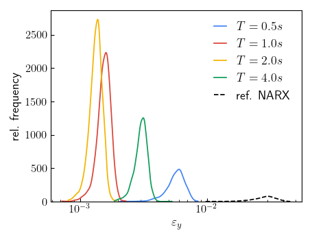
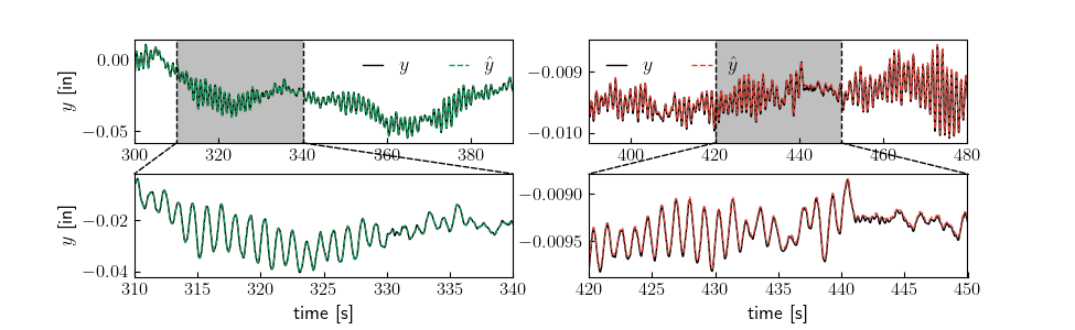
The performance of the -NARX models and the reference NARX model on the eight-story building under wind load are visualized in Figure 3. To quantify the goodness of the models we calculate the normalized mean-squared error as in Eq. (39) with , and subsequently denoted as , for every trace in the validation dataset. In Figure 3a, we show the kernel density estimate the distribution of all the over the validation dataset for four different experimental design sizes . Consequently, the colored curves in this subplot correspond to the Models 1-4 from Table 2. We also show in black the error distribution of the reference NARX model for comparison. Sections of the output traces corresponding to the best and worst prediction of Model 4 (out of validation curves) are shown Figure 4 for illustration purposes. In Figure 3a it can be seen that in general -NARX tends to result in more than one order of magnitude error reduction w. r. t. the reference NARX model. It is also clear that -NARX models show a clear decreasing error trend with increasing experimental designs. Interestingly, even a single trace in the experimental design can yield relatively good approximation error, at the cost of a much larger trace-to-trace accuracy variability.
Figure 3b shows the -NARX performance for different values of the explained variance (see Eq. (33)). These models correspond to Models 4-9 in Table 2. It can be seen that a smaller or equal to results in a clear loss in model performance. Very good performance is achieved for and the model performs best for , showing that performance can be compromised if is chosen too large. This can be explained by the increased dimensionality in the regression step for large , which can still lead to overfitting, as we will discuss in more detail later. For small the model cannot capture enough information to approximate the system response.
The results for different memories are given in Figure 3c. The models in this figure correspond to Model 4 and Models 11 to 13 in Table 2. Similarly to the previous case, too small and too high values result in reduced performance, with best performance achieved for s which is about twice the first mode period of the building which is s. Analogous to the previous case, this phenomenon may result from the limited information available for very short memories and the large dimensionality and potential overfitting associated for very long memories.
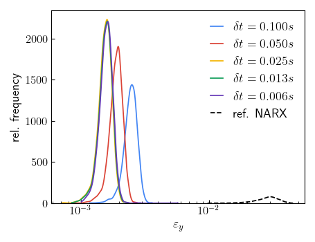
Finally, Figure 3d showcases the behavior of -NARX different sampling rates of the simulations, compared to the original sampling interval s. These correspond to Models 4 and 14 to 17 in Table 2. It is apparent that upsampling of the data does not affect the model performance. However, if the data is downsampled excessively, the performance starts decreasing. This is expected as high-frequency information in the data necessary to describe the system response can be lost.
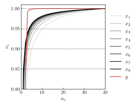
For a more thorough interpretation of the results from Figure 3, we plot the convergence of the explained variance for an increasing number of principal components and for each of the components (see Eq. (18)) in Figure 5a. Note that this plot corresponds to a memory of s with a sampling rate of 40 Hz as e. g. used for Model 4 in Table 2. We observe a fast initial increase in as gets larger. Consequently, most of the variance in the data can be explained by just a few components. The dimensionality during regression can thus be reduced significantly without much loss of information. As expected, the explained variances for converge at different rates, with the model response converging the fastest. Since was chosen homogeneously, variables that show slow convergence contribute more to the total dimensionality because they require more components to reach the target explained variance. It can therefore be beneficial to cover less variance of variables with slow convergence if they are found to be less important to the model response. An optimization of this trade-off could be performed through the DRSM approach introduced in Lataniotis et al. (2020), which performs a joint fit of the dimensionality reduction algorithm and surrogate model to improve the final surrogate accuracy.
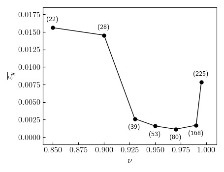
In Figure 5b we show the evolution of the average (average over the test simulations denoted as ) for increasing . For each data point, we annotate the corresponding number of regression coefficients, because it is expected to increase significantly with the explained variance . It can be observed that as increases, the model error first decreases with a large drop from to . This can be explained by the fact that the first principal components explain a lot of variance and these components may also be the most important ones to explain the response dynamics without increasing the dimensionality of the problem much (see Figure 5b). As sufficient information is available to explain the response dynamics, the error plateaus until it increases again at about . When approaches one, only comparatively little information is added by the extra input features, while the dimensionality increases rapidly and causes the model fitting to become underdetermined.
Note that the best value for for this problem lies within a relatively small window between and . However, choosing a value from this range appears natural due to the interpretability of this value. Alternatively, a plot such as shown in Figure 5b can help in choosing an appropriate value.
4.2 Three-story steel frame under seismic loading
In this application, we showcase the performance of -NARX on a realistic case study of a nonlinear three-story steel frame under seismic loading, which we adopted from Zhu et al. (2023). The frame structure is illustrated in Figure 6. Geometry parameters, basic material properties and the live load are listed in Table 3. For a detailed explanation of the model we refer to Zhu et al. (2023).
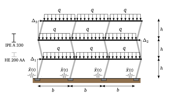
The quantities of interest are the three interstory drifts and (see Figure 6). The exogenous inputs are the ground acceleration , ground velocity and the ground displacement caused by seismic events. The ground acceleration data is taken from the Pacific Earthquake Engineering Research Center (PEER) database Power et al. (2008) which gathers recordings of earthquake data near the earth’s surface or on structure. In this case study we select earthquakes that leave the structure without significant permanent damage, as plastic deformation and damage accumulation would essentially require an infinite memory window. In turn, this behavior would make the problem unsuitable for a straightforward application of autoregressive modeling, which assumes finite system memory. Recent advancements on dynamic surrogate models, such as the recently introduced mNARX Schär et al. (2024), could in principle address this type of behavior, but it remains outside the scope of this work.
In total, we selected a rich set of acceleration recordings of real earthquakes sampled at Hz, covering near and far field, as well as low and high magnitude earthquakes. The ground motion velocity and displacement were obtained by direct numerical integration of the acceleration data. The simulations were performed using the open-source software OpenSees Pacific Earthquake Engineering Research Center (ease), and the resulting dataset was then randomly split into an experimental design comprising realizations and an out-of-sample test set of realizations for validation and performance assessment.
| Parameter | Unit | Value |
|---|---|---|
| Height | m | 3 |
| Width | m | 5 |
| Young’s modulus | MPa | |
| Yield stress | MPa | 235 |
| Live load | kN/m | 20 |
4.2.1 Model configurations
The configurations of the three final surrogates are shown in Table 4. These configurations were obtained by following a basis adaptive scheme as described in Section 4.1.1 using the hybrid LARS algorithm from Section 3.3. We tested polynomial degrees () from to , interaction orders () from to , and q-norms of , , and . We evaluated the forecast performance during LARS (Eq. (39)) at every -th iteration and stopped at a maximum of LARS iterations. Further, we only used a subset of samples of the full design matrix to reduce the computational cost during the model fitting process. The explained variances and memories were chosen identically for all three surrogates. They were also chosen homogeneously between the exogenous inputs and the autoregressive input, so we will subsequently omit the subscript. It is worth noting that the number of principal components required to achieve is considerably higher for the exogenous acceleration input than for the velocity and displacement . This is expected, since acceleration data carries higher frequencies than the corresponding velocities and displacements. The best configuration for all the surrogates has a polynomial degree of three but only for interaction terms were included. Remarkably, the final surrogate for is significantly sparser (only 19 non-zero coefficients) compared to the other two surrogates.
| Quantity of interest | |||
|---|---|---|---|
| Memory () | s | s | s |
| Explained variances () | |||
| # principal components (,,,) | /// | /// | /// |
| Maximum polynomial degree () | |||
| Maximum interaction order () | |||
| Q-norm () | |||
| # non-zero coefficients / # coefficients | / | / | / |
4.2.2 Results
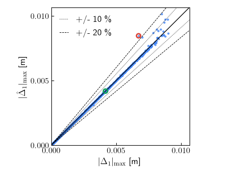
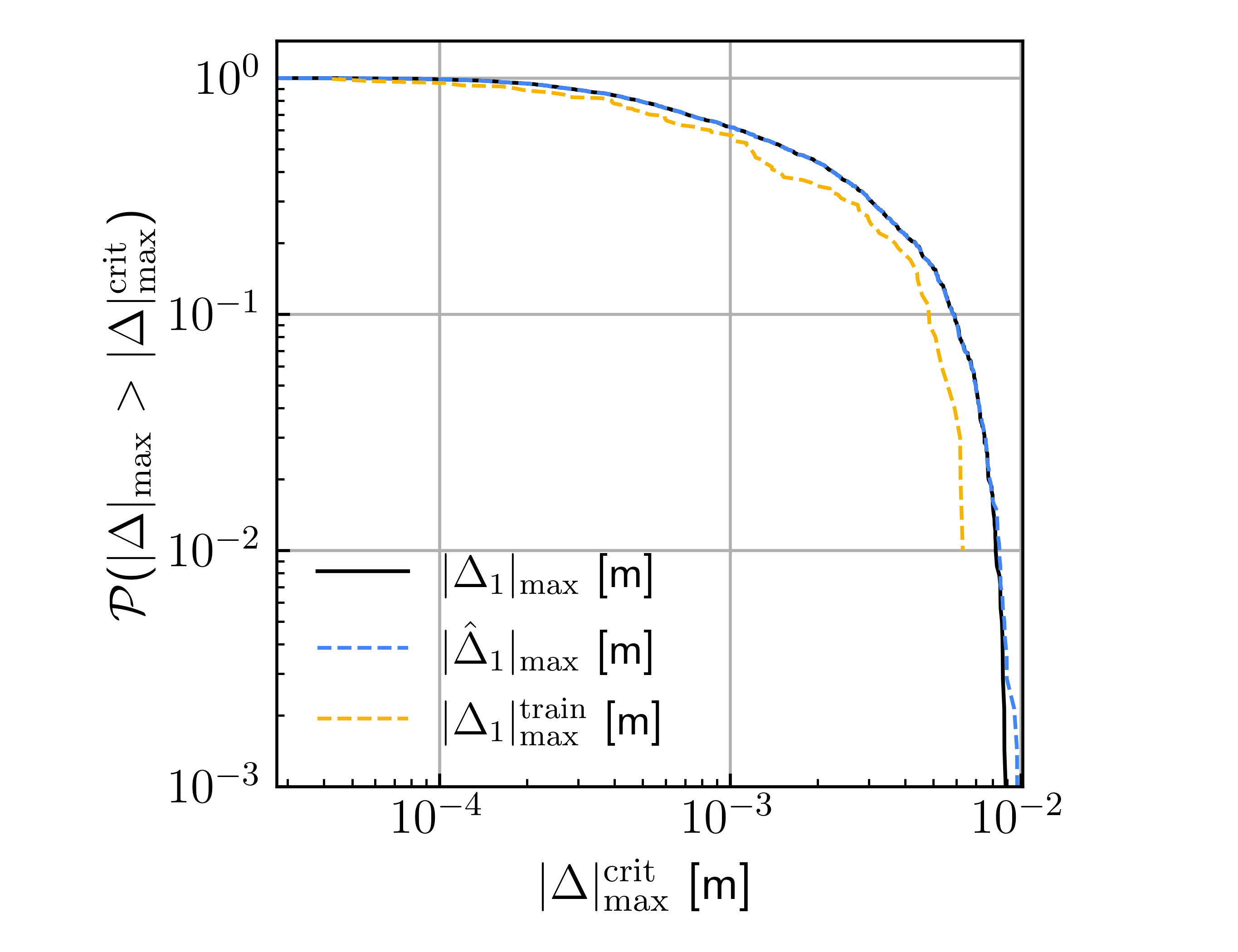
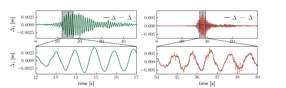
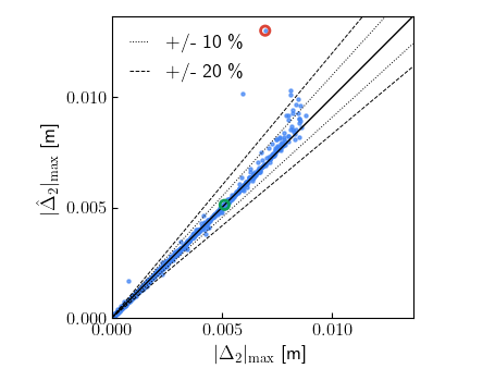
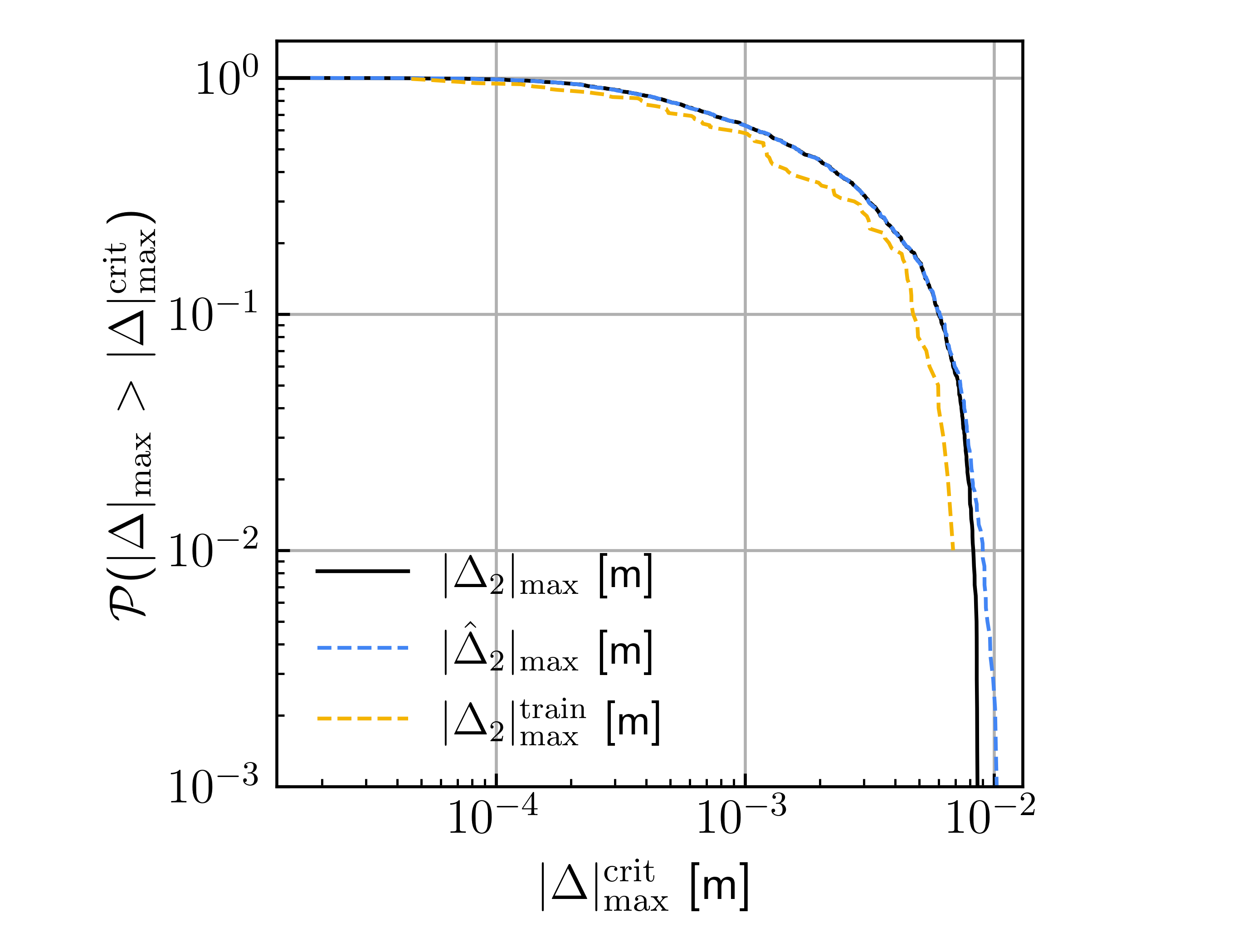
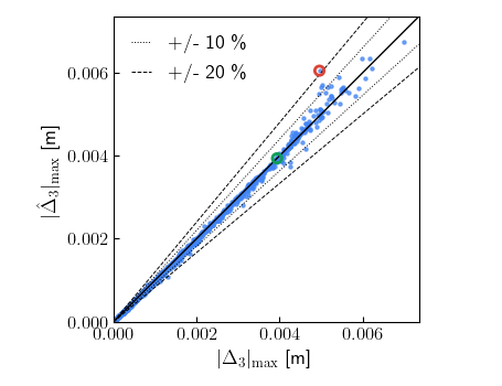
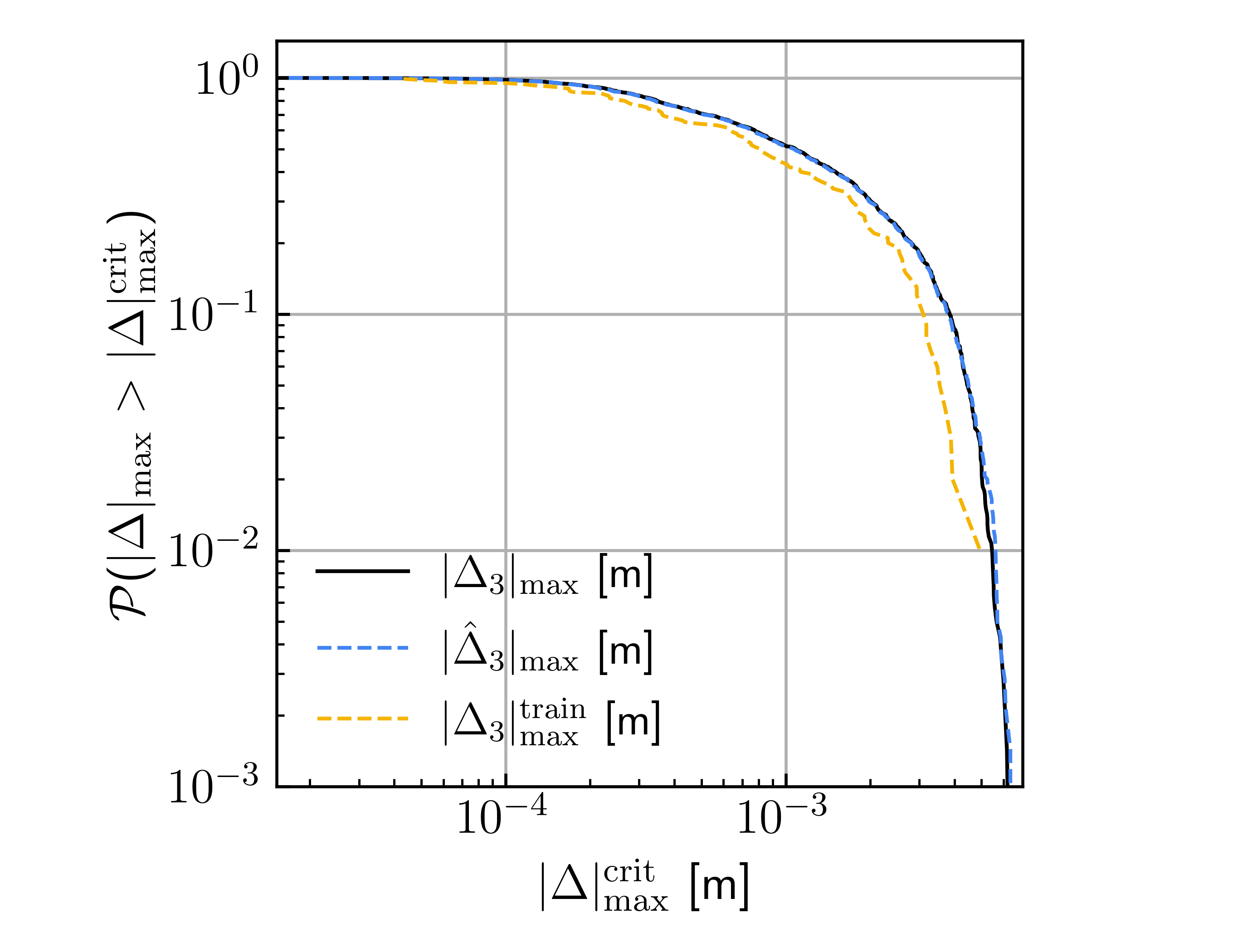
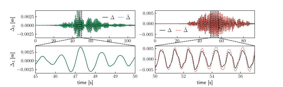
The results of the -NARX surrogates on the three-story steel frame case study are shown in Figures 7-9. Figure 7a compares the predictions of the -NARX model on the out-of-sample set of simulations for the 1 floor interstory drift, in terms of absolute peak drift, a quantity traditionally extremely difficult to approximate due to its highly non-linear and phase-sensitive nature. It can be seen that the absolute peak interstory drifts of the predicted traces align well with the reference ones. For most simulations, the discrepancy is within the 10 % error bounds, with only a handful of outliers with up to 30 % error in the far right tail. Figure 7b shows the corresponding survival plot with respect to a critical maximum drift , calculated from the true and predicted drifts. The predicted curve matches the reference up to an exceedance probability of about , with a mild deviation for lower probabilities. For reference, the same curve computed from the training traces is provided, and as expected it clearly deviates from the reference already for relatively high exceedance probabilities because of the limited dataset. For visualization purposes, we also show two traces of two example simulations in Figure 7c, in which the left and right traces have a low and high prediction error in , respectively. The predicted trace with the low error aligns almost perfectly with the reference over the full simulation duration, while the other is generally stable over the full signal duration, but shows spurious higher frequency oscillations in the range of the extreme drift values.
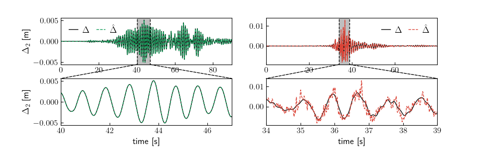
Figures 8a-c show the same results for the 2 floor interstory drift. The results are mostly comparable to the ones for the 1 floor, albeit with an overall lower accuracy, especially in the high tail of the distribution. The discrepancy in is significantly higher, which is reflected in the higher dispersion of the points in Figures 8a and the earlier divergence between the true and predicted survival curves in Figures 8b. The worse performance on the 2 floor interstory drift may be due to more complex dynamics, which are also reflected in the higher polynomial degree and interaction terms listed in Table 4.
Finally, we show the results for the 3 floor interstory drift in Figures 9a-c, which show an overall better agreement to the reference with respect to the previous two cases. The fact that the surrogate predicting the 3 floor has only non-zero model coefficients (see Table 4) indicates that the dynamics of this floor are indeed somewhat less complex to predict than the others.
5 Discussion and Conclusion
In this paper, we present a novel approach to nonlinear autoregressive with exogenous inputs (NARX) modeling, called -NARX for functional NARX. By following a continuous functional view point, rather than the well-established discrete-time approach, -NARX overcomes several limitations of traditional NARX models, making it particularly well-suited for surrogate modeling of dynamical physical systems, such as engineering structures, also in the presence of multiple exogenous inputs. -NARX addresses the sensitivity of classical NARX models to time discretization, their tendency to over-rely on recent autoregressive inputs, and their inefficiency in handling systems with long memory. These challenges are mitigated by modeling the system dynamics in a transformed space that captures key physical features from both the exogenous inputs and the autoregressive input (focus on functional features) rather than relying on original discrete time steps (focus on time discretization).
To validate the methodology, we chose a combination of feature extraction using principal component analysis and sparse polynomial NARX modeling based on hybrid LARS, and applied it to two different case studies intended to showcase both the robustness of the method w. r. t. the limitations of classical NARX, and its performance in the presence of a complex computational model.
In the first case study, we examined the behavior of -NARX applied to an eight-story building subjected to wind loading. The goal of this case study was to investigate the behavior of -NARX with respect to its configuration parameters. We demonstrated that the model is straightforward to parameterize using interpretable configuration parameters, and at the same time that it is largely unaffected by changes in the sampling rate of the simulations, enabling it to handle highly oversampled signals effectively.
In a challenging second case study, involving a nonlinear finite element model of a three-story steel frame under seismic loading, we demonstrated -NARX’s capability to accurately model more complex dynamical systems. The -NARX models accurately predicted the interstory drifts of the building over extended periods, despite being trained on a small experimental design of only 100 simulations. This forecast stability is largely due to the modeling of the system in the transformed feature space, which reduces the over-reliance on individual recent past output time steps that are highly correlated with the current output value.
The -NARX methodology, when deployed using PCA, polynomial basis functions with a basis adaptive scheme, and a sparse solver, proved to be a powerful surrogate for modeling complex dynamical systems typical of engineering simulation. Moreover, this implementation maintains low computational costs during model forecasting, making it practical for surrogate modeling. For the more complex second case study, the cost of the entire model fitting, including basis adaptivity, was in the order of hours on a standard notebook. This time strongly depends on the size of the experimental design, as most of the time is spent in the modified LARS algorithm to evaluate the forecast performance on the experimental design (see Section 3.3). The time taken to predict the validation traces was about minutes, which is approximately two orders of magnitude faster than the hours required to run the corresponding OpenSees simulations.
Future research can explore the integration of other feature extraction algorithms and their synergy with different basis functions. Additionally, leveraging prior system knowledge to construct features relevant to the system response is a promising avenue. As shown by Schär et al. (2024), incorporating expert knowledge into the modeling process can significantly improve the emulation of complex dynamical systems.
Declaration of Competing Interest
The authors declare that they have no known competing financial interests or personal relationships that could have appeared to influence the work reported in this paper.
Acknowledgments
This project is part of the HIghly advanced Probabilistic design and Enhanced Reliability methods for high-value, cost-efficient offshore WIND (HIPERWIND) project and has received funding from the European Union’s Horizon 2020 Research and Innovation Programme under Grant Agreement No. 101006689.
The authors express their sincere appreciation to Jungho Kim, Sang-ri Yi and Junho Song for their valuable contribution to the first case study by providing the corresponding numerical codes.
References
- Acuña et al. (2012) Acuña, G., C. Ramirez, and M. Curilem (2012). Comparing NARX and NARMAX models using ANN and SVM for cash demand forecasting for ATM. In The 2012 International Joint Conference on Neural Networks (IJCNN), pp. 1–6.
- Aguirre and Billings (1993) Aguirre, L. and S. Billings (1993). Relationship between the structure and performance of identified nonlinear polynomial models. Research report.
- Aguirre (1994) Aguirre, L. A. (1994). Some remarks on structure selection for nonlinear models. International Journal of Bifurcation and Chaos 4(6), 1707–1714.
- Aguirre and Billings (1995) Aguirre, L. A. and S. A. Billings (1995). Improved structure selection for nonlinear models based on term clustering. International Journal of Control 62(3), 569–587.
- Aguirre and Jácome (1998) Aguirre, L. A. and C. Jácome (1998). Cluster analysis of NARMAX models for signal-dependent systems. IEE Proceedings - Control Theory and Applications 145, 409–414(5).
- Awtoniuk et al. (2019) Awtoniuk, M., M. Daniun, K. Sałat, and R. Sałat (2019). Impact of feature selection on system identification by means of NARX-SVM. MATEC Web of Conferences 252, 03012.
- Ayala et al. (2017) Ayala, J., H. Wei, and S. Billings (2017). A novel logistic-NARX model as a classifier for dynamic binary classification. Neural Computing and Applications.
- Badeau et al. (2004) Badeau, R., G. Richard, and B. David (2004). Sliding window adaptive SVD algorithms. IEEE Transactions on Signal Processing 52(1), 1–10.
- Bastiaans (1985) Bastiaans, M. (1985). On the sliding-window representation in digital signal processing. IEEE Transactions on Acoustics, Speech, and Signal Processing 33(4), 868–873.
- Bengio et al. (2006) Bengio, Y., O. Delalleau, N. Le Roux, J.-F. Paiement, P. Vincent, and M. Ouimet (2006). Spectral Dimensionality Reduction, pp. 519–550. Springer Berlin Heidelberg.
- Bhattacharyya et al. (2020) Bhattacharyya, B., E. Jacquelin, and D. Brizard (2020). A Kriging–NARX model for uncertainty quantification of nonlinear stochastic dynamical systems in time domain. Journal of Engineering Mechanics 146(7), 04020070.
- Billings (2013) Billings, S. A. (2013). Nonlinear system identification: NARMAX methods in the time, frequency, and spatio-temporal domains. Chichester, West Sussex, United Kingdom: John Wiley & Sons, Inc.
- Billings and Aguirre (1995) Billings, S. A. and L. A. Aguirre (1995). Effects of the sampling time on the dynamics and identification of nonlinear models. International Journal of Bifurcation and Chaos 5(6), 1541–1556.
- Blatman and Sudret (2010) Blatman, G. and B. Sudret (2010). An adaptive algorithm to build up sparse polynomial chaos expansions for stochastic finite element analysis. Probabilistic Engineering Mechanics 25(2), 183–197.
- Blatman and Sudret (2011) Blatman, G. and B. Sudret (2011). Adaptive sparse polynomial chaos expansion based on least angle regression. J. Comput. Phys. 230(6), 2345–2367.
- Bracewell (1989) Bracewell, R. N. (1989). The Fourier transform. Scientific American 260(6), 86–95.
- Chen et al. (2008) Chen, S., X. X. Wang, and C. J. Harris (2008). NARX-based nonlinear system identification using orthogonal least squares basis hunting. IEEE Transactions on Control Systems Technology 16(1), 78–84.
- Chen and Ni (2011) Chen, Z. H. and Y. Q. Ni (2011). On-board identification and control performance verification of an MR damper incorporated with structure. Journal of Intelligent Material Systems and Structures 22(14), 1551–1565.
- Cheng et al. (2011) Cheng, Y., L. Wang, M. Yu, and J. Hu (2011). An efficient identification scheme for a nonlinear polynomial NARX model. Artificial Life and Robotics 16(1), 70–73.
- Chiras et al. (2001) Chiras, N., C. Evans, and D. Rees (2001). Nonlinear gas turbine modeling using NARMAX structures. IEEE Transactions on Instrumentation and Measurement 50(4), 893–898.
- Coca and Billings (2001) Coca, D. and S. A. Billings (2001). Non-linear system identification using wavelet multiresolution models. International Journal of Control 74(18), 1718–1736.
- Dassanayake et al. (2023) Dassanayake, S., A. Mousa, G. J. Fowmes, S. Susilawati, and K. Zamara (2023). Forecasting the moisture dynamics of a landfill capping system comprising different geosynthetics: A NARX neural network approach. Geotextiles and Geomembranes 51(1), 282–292.
- Deshmukh and Allison (2017) Deshmukh, A. P. and J. T. Allison (2017). Design of dynamic systems using surrogate models of derivative functions. Journal of Mechanical Design 139(10), 101402.
- Efron et al. (2004) Efron, B., T. Hastie, I. Johnstone, and R. Tibshirani (2004). Least angle regression. The Annals of Statistics 32(2), 407 – 499.
- Eldar and Kutyniok (2012) Eldar, Y. and G. Kutyniok (2012). Compressed Sensing: Theory and Applications. Compressed Sensing: Theory and Applications. Cambridge University Press.
- F. Bianchi and Piroddi (2017) F. Bianchi, A. Falsone, M. P. and L. Piroddi (2017). A randomised approach for NARX model identification based on a multivariate Bernoulli distribution. International Journal of Systems Science 48(6), 1203–1216.
- Falsone et al. (2014) Falsone, A., L. Piroddi, and M. Prandini (2014). A novel randomized approach to nonlinear system identification. In 53rd IEEE Conference on Decision and Control, pp. 6516–6521.
- Farina and Piroddi (2009) Farina, M. and L. Piroddi (2009). Simulation error minimization–based identification of polynomial input–output recursive models. IFAC Proceedings Volumes 42(10), 1393–1398.
- Farina and Piroddi (2010) Farina, M. and L. Piroddi (2010). An iterative algorithm for simulation error based identification of polynomial input–output models using multi-step prediction. International Journal of Control 83(7), 1442–1456.
- Gao et al. (2016) Gao, Y., S. Liu, F. Li, and Z. Liu (2016). Fault detection and diagnosis method for cooling dehumidifier based on LS-SVM NARX model. International Journal of Refrigeration 61, 69–81.
- Garg et al. (2022) Garg, S., H. Gupta, and S. Chakraborty (2022). Assessment of DeepONet for reliability analysis of stochastic nonlinear dynamical systems. arXiv:2201.13145.
- Hu et al. (2024) Hu, Z., J. Fang, R. Zheng, M. Li, B. Gao, and L. Zhang (2024). Efficient model predictive control of boiler coal combustion based on NARX neutral network. Journal of Process Control 134, 103158.
- Jolliffe (2002) Jolliffe, I. T. (2002). Principal Component Analysis. Springer-Verlag.
- Kim et al. (2023) Kim, J., S. Yi, and J. Song (2023). Estimation of first-passage probability under stochastic wind excitations by active-learning-based heteroscedastic Gaussian process. Structural Safety 100, 102268.
- Kim (2015) Kim, Y. (2015). Prediction of the dynamic response of a slender marine structure under an irregular ocean wave using the NARX-based quadratic Volterra series. Applied Ocean Research 49, 42–56.
- Kocijan (2012) Kocijan, J. (2012). Plenary lecture 1: Dynamic GP models: An overview and recent developments. In Proceedings of the 6th International Conference on Applied Mathematics, Simulation, Modelling, ASM’12, Stevens Point, Wisconsin, USA, pp. 12. World Scientific and Engineering Academy and Society (WSEAS).
- Koziel et al. (2014) Koziel, S., L. Leifsson, and X.-S. Yang (Eds.) (2014). Solving Computationally Expensive Engineering Problems: Methods and Applications, Volume 97. Springer International Publishing.
- Lacerda Junior et al. (2021) Lacerda Junior, W. R., S. A. M. Martins, and E. G. Nepomuceno (2021). Meta-model structure selection: Building polynomial narx model for regression and classification. arXiv:2109.09917.
- Langeron et al. (2021) Langeron, Y., K. T. Huynh, and A. Grall (2021). A root location-based framework for degradation modeling of dynamic systems with predictive maintenance perspective. Proceedings of the Institution of Mechanical Engineers, Part O: Journal of Risk and Reliability 235(2), 253–267.
- Lataniotis et al. (2020) Lataniotis, C., S. Marelli, and B. Sudret (2020). Extending classical surrogate modeling to high dimensions through supervised dimensionality reduction: A data-driven approach. International Journal for Uncertainty Quantification 10(1), 55–82.
- Levin and Narendra (1996) Levin, A. and K. Narendra (1996). Control of nonlinear dynamical systems using neural networks. II. Observability, identification, and control. IEEE Transactions on Neural Networks 7(1), 30–42.
- Li et al. (2021) Li, B., W.-C. Chuang, and S. M. J. Spence (2021). Response estimation of multi-degree-of-freedom nonlinear stochastic structural systems through metamodeling. Journal of Engineering Mechanics 147(11), 04021082.
- Li et al. (2021) Li, D., J. Zhou, and Y. Liu (2021). Recurrent-neural-network-based unscented Kalman filter for estimating and compensating the random drift of MEMS gyroscopes in real time. Mechanical Systems and Signal Processing 147, 107057.
- Loève (1955) Loève, M. (1955). Probability Theory. University series in higher mathematics. Springer-Verlag.
- Mai et al. (2016) Mai, C.-V., M. D. Spiridonakos, E. Chatzi, and B. Sudret (2016). Surrogate modeling for stochastic dynamical systems by combining nonlinear autoregressive with exogeneous input models and polynomial chaos expansions. Int. J. Uncertainty Quantification 6(4), 313–339.
- Mattson and Pandit (2006) Mattson, S. G. and S. M. Pandit (2006). Statistical moments of autoregressive model residuals for damage localisation. Mechanical Systems and Signal Processing 20(3), 627–645.
- Murray-Smith et al. (1999) Murray-Smith, R., T. A. Johansen, and R. Shorten (1999). On transient dynamics, off-equilibrium behaviour and identification in blended multiple model structures. In 1999 European Control Conference, pp. 3569–3574. IEEE.
- Olkkonen (2011) Olkkonen, J. T. (2011). Discrete Wavelet Transforms - Theory and Applications. IntechOpen.
- Pacific Earthquake Engineering Research Center (ease) Pacific Earthquake Engineering Research Center (Year of Software Release). OpenSees: Open System for Earthquake Engineering Simulation. Berkeley, CA: University of California, Berkeley.
- Pearson (1901) Pearson, K. (1901). LIII. On lines and planes of closest fit to systems of points in space. The London, Edinburgh, and Dublin Philosophical Magazine and Journal of Science 2(11), 559–572.
- Piroddi (2008) Piroddi, L. (2008). Simulation error minimisation methods for NARX model identification. International Journal of Modelling, Identification and Control 3, 392–403.
- Piroddi et al. (2010) Piroddi, L., V. Seghezza, and M. Bonin (2010). NARX model selection based on simulation error minimisation and LASSO. IET Control Theory & Applications 4(7), 1157–1168.
- Piroddi and Spinelli (2003) Piroddi, L. and W. Spinelli (2003). An identification algorithm for polynomial NARX models based on simulation error minimization. International Journal of Control 76(17), 1767–1781.
- Power et al. (2008) Power, M., B. Chiou, N. Abrahamson, Y. Bozorgnia, T. Shantz, and C. Roblee (2008). An overview of the NGA project. Earthquake Spectra 24(1), 3–21.
- Pulecchi and Piroddi (2007) Pulecchi, T. and L. Piroddi (2007). A cluster selection approach to polynomial NARX identification. In 2007 American Control Conference, pp. 852–857.
- Ramin et al. (2023) Ramin, V. P., H. G. Amin, and N. Alireza (2023). An investigation of the performance of the ANN method for predicting the base shear and overturning moment time-series datasets of an offshore jacket structure. International Journal of Sustainable Construction Engineering and Technology 14(4), 79–93.
- Ranković et al. (2014) Ranković, V., N. Grujović, D. Divac, and N. Milivojević (2014). Development of support vector regression identification model for prediction of dam structural behaviour. Structural Safety 48, 33–39.
- Rumelhart and McClelland (1986) Rumelhart, D. E. and J. L. McClelland (1986). Parallel distributed processing: explorations in the microstructure of cognition. Computational models of cognition and perception. MIT Press.
- Samsuri et al. (2023) Samsuri, N. A., S. A. Raman, and T. M. Y. S. Tuan Ya (2023). Evaluation of NARX network performance on the maintenance application of rotating machines. In F. Ahmad, H. H. Al-Kayiem, and W. P. King Soon (Eds.), ICPER 2020, Singapore, pp. 593–609. Springer Nature Singapore.
- Schlechtingen and Ferreira Santos (2011) Schlechtingen, M. and I. Ferreira Santos (2011). Comparative analysis of neural network and regression based condition monitoring approaches for wind turbine fault detection. Mechanical Systems and Signal Processing 25(5), 1849–1875.
- Schär et al. (2024) Schär, S., S. Marelli, and B. Sudret (2024). Emulating the dynamics of complex systems using autoregressive models on manifolds (mNARX). Mechanical Systems and Signal Processing 208, 110956.
- Siegelmann et al. (1997) Siegelmann, H., B. Horne, and C. Giles (1997). Computational capabilities of recurrent NARX neural networks. IEEE Transactions on Systems, Man, and Cybernetics, Part B (Cybernetics) 27(2), 208–215.
- Song et al. (2022) Song, H., X. Shan, L. Zhang, G. Wang, and J. Fan (2022). Research on identification and active vibration control of cantilever structure based on NARX neural network. Mechanical Systems and Signal Processing 171, 108872.
- Spinelli et al. (2006) Spinelli, W., L. Piroddi, and M. Lovera (2006). A two-stage algorithm for structure identification of polynomial NARX models. In 2006 American Control Conference, pp. 2387–2392.
- Spiridonakos and Chatzi (2015) Spiridonakos, M. D. and E. N. Chatzi (2015). Metamodeling of nonlinear structural systems with parametric uncertainty subject to stochastic dynamic excitation. Earthquakes and Structures 8(4), 915–934.
- Strang and Nguyen (1996) Strang, G. and T. Nguyen (1996). Wavelets and Filter Banks. Philadelphia, PA: Wellesley-Cambridge Press.
- Sundararajan (2001) Sundararajan, D. (2001). The Discrete Fourier Transform: Theory, Algorithms and Applications. World Scientific.
- Tenenbaum et al. (2000) Tenenbaum, J. B., V. de Silva, and J. C. Langford (2000). A global geometric framework for nonlinear dimensionality reduction. Science 290(5500), 2319–2323.
- Tibshirani (1996) Tibshirani, R. (1996). Regression shrinkage and selection via the lasso. Journal of the Royal Statistical Society. Series B (Methodological) 58(1), 267–288.
- Verleysen and François (2005) Verleysen, M. and D. François (2005). The curse of dimensionality in data mining and time series prediction. In Proceedings of the 8th International Conference on Artificial Neural Networks: Computational Intelligence and Bioinspired Systems, IWANN’05, Berlin, Heidelberg, pp. 758–770. Springer-Verlag.
- Wei and Billings (2008) Wei, H. L. and S. A. Billings (2008). Model structure selection using an integrated forward orthogonal search algorithm assisted by squared correlation and mutual information. International Journal of Modelling, Identification and Control 3(4), 341.
- Worden and Barthorpe (2012) Worden, K. and R. J. Barthorpe (2012). Identification of hysteretic systems using narx models, part I: Evolutionary identification. In Topics in Model Validation and Uncertainty Quantification, Volume 4, pp. 49–56. Springer New York.
- Worden et al. (2018) Worden, K., W. Becker, T. Rogers, and E. Cross (2018). On the confidence bounds of Gaussian process NARX models and their higher-order frequency response functions. Mechanical Systems and Signal Processing 104, 188–223.
- Wunsch et al. (2018) Wunsch, A., T. Liesch, and S. Broda (2018). Forecasting groundwater levels using nonlinear autoregressive networks with exogenous input (NARX). Journal of Hydrology 567, 743–758.
- Yetkin et al. (2017) Yetkin, M., M.-S. Kim, and Y. Kim (2017). Mooring line top-tension prediction using NARX. International Ocean and Polar Engineering Conference, pp. ISOPE–I–17–375.
- Yu et al. (2023) Yu, C., Y.-P. Zhu, H. Luo, Z. Luo, and L. Li (2023). Design assessments of complex systems based on design oriented modelling and uncertainty analysis. Mechanical Systems and Signal Processing 188, 109988.
- Yuzhu Guo and Wei (2015) Yuzhu Guo, L.Z. Guo, S. B. and H.-L. Wei (2015). An iterative orthogonal forward regression algorithm. International Journal of Systems Science 46(5), 776–789.
- Zhang et al. (2017) Zhang, J., Z. Yin, and R. Wang (2017). Nonlinear dynamic classification of momentary mental workload using physiological features and NARX-model-based least-squares support vector machines. IEEE Transactions on Human-Machine Systems 47(4), 536–549.
- Zhang et al. (2024) Zhang, L., S. Draycott, and P. Stansby (2024). System identification and generalisation of elastic mooring line forces on a multi-float wave energy converter platform in steep irregular waves. Mechanical Systems and Signal Processing 214, 111259.
- Zhang et al. (2024) Zhang, Y., Y. Dong, and M. Beer (2024). rLSTM-AE for dimension reduction and its application to active learning-based dynamic reliability analysis. Mechanical Systems and Signal Processing 215, 111426.
- Zhou and Li (2023) Zhou, J. and J. Li (2023). An efficient time-variant reliability analysis strategy embedding the NARX neural network of response characteristics prediction into probability density evolution method. Mechanical Systems and Signal Processing 200, 110516.
- Zhu et al. (2023) Zhu, X., M. Broccardo, and B. Sudret (2023). Seismic fragility analysis using stochastic polynomial chaos expansions. Probabilistic Engineering Mechanics 72(103413).