A five-dimensional Lorenz-type model near the temperature of maximum density
Abstract
The current study formulates a convective model of the Lorenz type near the temperature of maximum density. The existence of this temperature actualizes water dynamics in temperate lakes. There is a conceptual interest what this feature induces in Lorenz-type models. The consideration starts with the zero coefficient of thermal expansion. Other steps are like famous Tritton’s approach to derive the Lorenz model. This allows us to reduce difficulties with a selection of Galerkin functions. The analysis focuses on changes induced by zeroing the coefficient of thermal expansion. It results in a five-dimensional Lorenz-type model, whose equations are all nonlinear. The new model reiterates many features of the standard Lorenz model. The nontrivial critical points appear, when the zero critical point becomes unstable. The nontrivial critical points correspond to two possible directions of fluid flow. Phase trajectories of the new model were studied numerically. The results are similar to the known five-dimensional extensions of the Lorenz model.
I Introduction
Hydrodynamic instabilities and the transition to turbulence are closely related problems with a long and wealthy history. The discovery of strange attractors has provided a new approach to understanding of the mechanisms by which turbulence may occur [1, 2]. Many of the results obtained in this way were stimulated by studies on the Lorenz model [3]. Edward Lorenz laid the foundation for what many consider the third revolution of 20th century — chaos theory [4]. The Lorenz model [5, 6] is recognized as a classic realization of a simple physical system with strange attractors. Following the ideas of Saltzman [7], it includes a quite successful combination of properly chosen Galerkin modes. The Lorenz equations used a very severe truncation of the equations of Bénard convection. It is well known that a larger number of Galerkin modes makes the model more adequate [8, 9, 10, 11]. In this way, the whole family of closely related models occurred. The dynamical system approach has found its right place in the theory of turbulence [12] and geophysical hydrodynamics [13, 14]. It turns out that low-order models are relevant to explore the scaling laws and mechanisms of the energy cascade.
Pursuing various aims of a physical or even mathematical origin, both simplified versions and generalizations of the standard Lorenz model have been considered in the literature. From the point of view of studying the structure of the Lorenz system itself, its truncated versions were examined. In particular, the limiting equations [3], the geometric model [15], and the nondissipative Lorenz model [16]. Among the extensions of the Lorenz system, models with a larger number of space modes in the temperature function are best known [9, 10]. Models with a larger selection of Galerkin modes in both the stream and temperature functions are also known [8, 11, 17]. Such models with an arbitrary number of functions are rather the subject of numerical procedures. However, in all of the listed cases, the thermal expansion coefficient was assumed to be nonzero. In contrast, this study aimed to consider a Lorenz-type model with zero coefficient of thermal expansion. There are several reasons to accomplish this consideration. Changes in the mathematical properties of the corresponding dynamical models are interesting themselves. On the other hand, there is a physical reason to deal with this question.
Substances common in everyday life typically undergo thermal expansion in response to heating. In other words, a given mass of a substance expands to a larger volume when its temperature increases. Nevertheless, the coefficient of thermal expansion of some substances can principally change the sign under certain conditions. Water, especially important for Life, is also notable as having the maximum density at temperatures near C [18]. Of course, the exact value of the temperature of maximum density of natural water depends on actual pressure and salinity. In fact, the annual evolution of stratification in temperate lakes according to Forel’s classification [19] is a shining manifestations of the existence of this temperature. When salinity effects are negligible, the temperatures of the upper layer of a lake cross the point of maximum density twice in a year (see, e.g., subsection 1.3.1 of Ref. [20]). The Great Lakes [21] are an especially famous example. Lake Baikal known for its outstanding features [22] undergoes a regular annual alternation of summer and inverse winter stratification [23]. There is a domain in the upper layer where any linear relation between the density and temperature of water becomes inadequate [22].
This study aims to examine changes in Lorenz-type systems near the point of maximum density. The addressed question is interesting from its own perspective and for applications in which the temperature of maximum density plays an important role. Then, a buoyancy term proportional to the square of excess temperature should be considered. To investigate the question of interest, the coefficient of thermal expansion was assumed to be zero in the setup. The proposed model differs from all previous models by a nonlinear term in the first equation, which succeeds the Navier–Stokes vector equation. In effect, the obtained five-dimensional system contains only nonlinear equations. To dive into the essence of the problem, we treat it similarly to Tritton’s physics-based approach to derive the Lorenz model [24]. This way allows us to mitigate difficulties with selecting the required Galerkin functions. In a more complete description, these functions satisfy the imposed boundary conditions. This makes their selection more difficult than in our adaptation of Tritton’s approach.
This paper is organized as follows. Section II describes the physical basis of the model of interest. The accepted form of the buoyancy term directly leads to a momentum equation with nonlinearity in temperature deviations. In terms of properly chosen dimensionless units, five differential equations with quadratic nonlinearity appear in Sec. III. The basic points of the analysis of the proposed model are presented in Sec. IV. In particular, we derive nontrivial critical points and discuss conditions for their existence. As will be shown, the situation that occurs in the standard Lorenz model is fully reproduced here. The numerical investigation results of the proposed model are described in Sec. V. They allow us to support analytical findings and analogies with the standard Lorenz model. In effect, projections on different planes in phase space illustrate the existence of attracting orbits. This situation is similar to that held for the known five-dimensional extension of the standard model. Section VI concludes the paper with a summary of the reported results. The stability of nontrivial critical points is considered in Appendix A.
II Physical basis of the model
Thermally induced convection is one of important directions of researches in physics of fluids as well as in some engineering disciplines. It is typically considered within the Boussinesq approximation, different aspects of which are examined thoroughly in Refs. [25, 26, 27]. Rayleigh–Bénard convection is studied in detail due to its analytical [28, 29] and experimental accessibility [30, 17]. To study turbulence in thermal convection, theoretical analysis [31, 32] is typically combined with experimental data [33, 34, 35, 36, 37] and numerical simulation [38, 39, 40, 41, 42]. Most of the results were obtained for the case with the strictly positive coefficient of thermal expansion. This coefficient reads as
| (1) |
where is the density, is the temperature, and is the pressure.
In contrast to typical situation with , the so-called thermal contraction is also allowed in thermodynamics. In this regard, the thermal expansion coefficient differs from the coefficient of isothermal compressibility. The latter should be positive due to classical thermodynamic (see, e.g., §21 of Ref. [43]). On the other hand, thermodynamic demonstrations that compressibility must be positive all appear to deal with additional assumptions [44]. These circumstances show that convection with vanishing deserves to be considered a fortiori. Convective motions in water near the point of maximum density have already found some coverage [45, 46]. The aim of the current study is to focus on other aspects. What happens in models of the Lorenz type with zero ? Thus, we will further use a thermodynamic equation of state in the form
| (2) |
By and , we mean here the temperature of maximum density and the corresponding strictly positive factor. Variations of height are assumed to be so small that their influence on the temperature of maximum density is negligible.
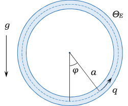
The physical system of interest is shown in Fig. 1. The fluid moves in a vertically placed loop of radius and fixed cross section. In contrast to Tritton’s approach to derive the Lorenz system in section 17.3 of Ref. [24], the thermodynamic equation of state reads as (2). Tritton’s reformulation is similar to the setup described in Ref. [47]. The position round the loop is described by the angle . It is now necessary to choose a profile of the external temperature. It often occurs in physics that formulations with arbitrary functions on the boundaries are difficult to tractable immediately. Then expansions of some kind are typically used, for instance, the Taylor series expansion. At least as the first step, the number of involved terms is restricted to take into account nontrivial effects. It is helpful to recall that the Lorenz system per se was built with minimal number of Galerkin functions required to include a part of nonlinearities of the initial equations. In this sense, the simplest model of the whole family of ones is selected as the starting point. It is well known that low-order models are physically sound in various respects [51, 52]. A limited number of involved equations can be enough to understand the scaling laws and mechanisms of the energy cascade at small scales [12].
According to the above reasons, the external temperature is taken to vary with height according to
| (3) |
where and are the prescribed constants. In other words, the quantity is expanded up to the term quadratic in the height deviation from the mean level of the loop. We avoid to rewrite (3) explicitly in terms of the height deviation since only the values and will be used in the following. It will be shown that the quadratic term is required to make the consideration self-consistent. Dealing with quadratic functions is naturally suggested, when dependencies of the form (2) arise. The chosen form restricted to a quadratic term is the first that leads to nontrivial dynamics. In principle, more terms in the right side of (3) could be kept in future investigations.
It is assumed that the variations in velocity and temperature over a cross section may be handled by working in terms of an average speed and average temperature . The speed is taken positive, when flow is anticlockwise. The continuity equation corresponds to the Boussinesq approximation, viz.
| (4) |
Hence, depends on time only [24]. The Navier–Stocks equation reduces to the form that reflects the momentum balance. Within the Tritton approach, it reads as
| (5) |
Following Ref. [24], the term with is placed in the right-hand side of (5). Thereby, the action of viscosity is supposed to induce a resistance to the motion proportional to its speed. Like the Boussinesq approximation, density changes are taken into account only in the third term in the right-hand side of (5). It is valid since actual vertical acceleration is very small in comparison with the gravitational one. Substituting (2) into (5) and integrating with respect to results in
| (6) |
The last term in the right-hand side of (6) replaces the integral
| (7) |
which is used in Tritton’s formulation. The term with the coefficient of thermal expansion commonly appears within the Boussinesq approximation. The current study aims to examine changes due to zero . These changes are now reflected in the right-hand side of (6).
The fluid temperature inside the loop is represented in the form
| (8) |
Tritton’s approach [24] uses only the first two terms in the right-hand side of (8). It will be shown soon that two additional trigonometric functions are needed to take into account an influence of buoyancy near the temperature of maximum density. The second term in the left-hand side of (11) generates sines from cosines, and vice versa. In contrast to (3), therefore, the two sine functions stand in (8). Note also that our notation slightly differs from that was used in section 17.3 of Ref. [24]. The expansion (8) can be interpreted as a very simple example of Galerkin methods widely used in computational fluid dynamics [48]. Substituting for the usual ansatz , the integral in the right-hand side of (6) vanishes. Indeed, one easily obtain
| (9) |
It is for this reason that we put two additional terms into the right-hand side of (8). Elementary calculations give two nonzero contributions, so that we reduce (6) to the form
| (10) |
This equation reflects a balance of the momentum.
Following Tritton’s formulation [24], the temperature evolves as
| (11) |
Here, the right-hand side supposes that heat is transferred through the walls at a rate proportional to the local difference between the external temperature and the average internal temperature. Substituting (3) and (8) into (11) gives
| (12) |
Treating these expressions as Fourier series, one gets
| (13) | ||||
| (14) | ||||
| (15) | ||||
| (16) |
It is convenient to introduce new variables and , so that
| (17) | ||||
| (18) | ||||
| (19) | ||||
| (20) |
Using and allows one to rewrite the momentum equation (10) as
| (21) |
The equations (17)–(21) present the basis of the novel Lorenz-type model of thermal convection near the temperature of maximum density.
III Dimensionless equations and control parameters
It is commonly accepted to reformulate equations of the above type in dimensionless units. Together with this reformulation, proper control parameters of the new model will be extracted here. Some inspection allows one to accomplish a natural way to put dimensionless units. We refrain from presenting some details here and provide only final expressions. Let us introduce dimensionless time and dimensionless functions, so that
| (22) | ||||
| (23) | ||||
| (24) | ||||
| (25) | ||||
| (26) |
The first expression is the same that appears in Tritton’s formulation. Other expressions differ since the unit of temperature should be put in other way due to zero . Namely, the factor standing right before each temperature function in (23)–(26) replaces the factor
| (27) |
The control parameters are respectively defined as
| (28) | ||||
| (29) | ||||
| (30) |
Within Tritton’s approach [24], the parameter (28) plays the role of the Prandtl number. By definition, both the parameters and cannot be negative, but may vanish. Finally, the five dimensionless equations of the new model are obtained as follows:
| (31) | ||||
| (32) | ||||
| (33) | ||||
| (34) | ||||
| (35) |
The equation (31) represents (21), whereas the equations (32)–(35) represent (17)–(20), respectively. In contrast to generalized Lorenz models used in Refs. [8, 9, 10], the first equation of the new system is genuinely nonlinear. This fact follows from the equation of state (2) chosen to focus on vicinity of the maximum density. Thus, the key distinction of the proposed model consists of nonlinearity with respect to temperature functions in the equation that reflects a momentum balance. The additional equations (34) and (35) are very similar to (32) and (33), respectively. The only distinctions are the factor and the term in the right-hand side of (34) with the control parameter . It will be seen that the equations (32) and (33) respectively correspond to the second and third equations appeared in Tritton’s formulation. In this sense, we developed its version suitable near the temperature of maximum density. The analysis of the critical points will be accomplished in the next section. In essence, the picture that occurs in the standard Lorenz model is also reproduced with the new model.
It is instructive to recall briefly the three equations appeared in Tritton’s approach. Then the dimensionless time and are defined just as above. The definitions (23) and (24) should be rewritten with the factor (27) standing right before the corresponding temperature function. In dimensionless variables, the equations read as
| (36) | ||||
| (37) | ||||
| (38) |
where the control parameter
| (39) |
Here, the denominator is of acceleration dimension. Formally, the equations (32) and (33) of the new system resemble (37) and (38), respectively. Indeed, the temperature equation (11) is the same as in Tritton’s approach. This equation replaces the heat flow equation commonly used in the Boussinesq approximation. To obtain the standard Lorenz model [5] as it commonly appears, the right-hand side of (38) is rewritten with instead of . Also, the parameter should be treated as the Prandtl number.
Convective models with a truncation different from the Lorenz truncation have already been quoted above. There are a lot of closely related models developed for various purposes. The five-mode model of thermohaline convection proposed by Veronis [49] uses a similar truncation of modes. The Lorenz model can be obtained within the concept of Volterra gyrostats [50, 51, 52]. The standard Lorenz model was also reformulated in the sense of modulated control parameters [53, 54, 55]. In addition, the authors of Ref. [55] compared their findings with the experimental data reported in Ref. 56. An eight-mode model for convection in binary mixtures was examined in Refs. [57, 58]. It must be stressed that the system (31)–(35) differs from all the mentioned models by nonlinearity in the first equation for dimensionless acceleration. At the same time, the new model of convection can also be recast in these respects. Questions of such a kind are beyond the present consideration. In this paper, we aim to concentrate on the system (31)–(35) and its principal properties.
IV Critical points
The common approach to models of the considered type is to obtain critical points and investigate their stability. Critical points are defined as fixed ones, e.g., as solutions to the system of algebraic equations derived from (31)–(35) without dependence on time. Thus, we have
| (40) | ||||
| (41) | ||||
| (42) | ||||
| (43) | ||||
| (44) |
Substituting immediately gives . Let us mention briefly the physical interpretation of the zero critical point. This solution corresponds to the fluid remaining at rest in the loop. The fluid temperature inside the loop is constant and equal to the external temperature at the given height. Due to (24) and (26), the formulas and respectively give and . Combining the latter with really implies that (8) reduces to (3). Of course, this solution for the state at rest can directly be obtained from (11).
It is clear that nontrivial critical points are allowed only for . It follows from (41) and (42) that
| (45) |
In a similar manner, the equations (43) and (44) give
| (46) |
Due to (45) and (46), it holds that
| (47) |
Since , the first equation of our system leads to
| (48) |
Thus, we obtain the quadratic equation
| (49) |
which should be solved for . To exclude imaginary and zero values for , we require . By a little algebra, one has
| (50) |
Nontrivial critical points exist under the condition
| (51) |
It is interesting that both the control parameters should be nonzero. Moreover, the obtained constraint is a reminiscent of complementarity relation between the position and momentum spreads due to Heisenberg’s uncertainty principle. Let one of the two control parameters decreases. To ensure the existence of nontrivial critical points, other parameter should increase properly. In terms of initial quantities, the condition (51) reads as
| (52) |
Critical points of the standard model (36)–(38) are obtained as follows. Equating the right-hand sides to zero, one gets the system of three algebraic equations. The zero critical point exists for all values of . For , there are the two additional solutions with . The fact that and have the same sign implies that in each case hot fluid is rising and cold fluid falling [24]. In terms of initial quantities, the condition reads as
| (53) |
The condition (52) obtained for the new model is similar to the condition (53).
Of course, analytic expressions for the critical points of our five-dimensional system are more complicated. As a result of calculations due to (45) and (46), we have the two points , where
| (54) |
These solutions correspond to the fluid circulating in the loop at a constant speed and with a constant temperature distribution. The different signs in the first mode representing average velocity correspond to two possible directions of circulation, anticlockwise and clockwise. Like nontrivial steady-state solutions of the standard model, the sign of the second and forth modes is the same as the sign of the first. And as before, the third and fifth modes multiplied by cosine functions in (8) are always positive.
Let us examine stability of the solution without motion. Suppose that all the variables are small and proportional to . Substituting this into the system (31)–(35) and neglecting nonlinear terms, we obtain
| (55) |
The latter is the characteristic equation with the sign minus. Calculating the determinant of matrix leads to the characteristic equation
| (56) |
where
| (57) |
The eigenvalue has multiplicity three. Only can have strictly positive real part, and this happens under the condition (51). Thus, the zero critical point becomes unstable simultaneously with the appearance of nontrivial critical points. Both these points represent steady solutions with constant flow in the loop. Thus, the situation that occurs in the standard Lorenz model is also reproduced here. As the product of control parameters increases properly, the state without motion loses stability so that a convection is being.
Stability of nontrivial critical points is more complicated to analyze explicitly. To avoid diving into calculations here, main details are presented in Appendix A. It will be more instructive to discuss the physical meaning of an irregular behavior, when the steady solutions become unstable. This instability has a different character from the instability of the zero point that represents fluid in the rest. In the absence of any stable steady solutions, some kind of unsteady motion must occur anyway. It will be exemplified in the next section that oscillations of increasing amplitude take place. Growing pulsations of the flow are superimposed on the mean circulation. At once, observed trajectories still lie in a finite domain of the phase space. This property indeed holds thought it does not follow from numerical results alone. This regime shows seemingly random “transitions” between neighborhoods of the two nontrivial critical points. From a physical viewpoint, this means a sudden change in the direction of fluid circulation in the loop. We see again that a typical situation occurring in the Lorenz system is resembled. The results of this section show that the proposed model is physically meaningful and consistent.
V Numerical results
This section presents the numerical analysis results of the proposed system (31)–(35). Of course, emphasis should be given here to chaotic dynamics in the case of unstable critical points. The calculations were also performed for cases when both steady solutions were stable. They completely supported the predictions based on linear stability analysis. If only the zero critical point is unstable, the perturbations grow monotonically until a point in the phase space is attracted by one of the nontrivial critical points. In the following, we visualize the trajectories between the neighborhoods of two nontrivial critical points. Since five modes are involved, the points in the phase space include five coordinates. Hence, the picture cannot be shown fully, even in three dimensions. The role of the visualization of phase space for understanding bifurcations such as those occurring in the Lorenz system was emphasized in Ref. [59]. Following the original paper of Lorenz [5], we shall characterize dynamics by showing projections on different planes.
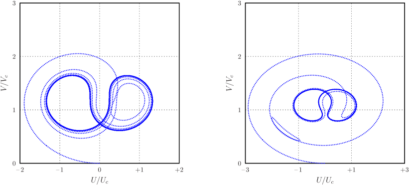
The equations are integrated forward in time with the use of the classic fourth-order Runge–Kutta formula (see, e.g., section 17.1 of Ref. [60]). We refrain from presenting the well-known content of this scheme. To obtain the results, one uses iterations of the fourth-order Runge–Kutta scheme with the value for dimensionless time increment. Thus, the total interval contains dimensionless time units. To check the stability of the numerical integration, calculations were tested with various numbers of steps and increments. Examples of projections on different planes are presented in Figs. 2–5 for the following two choices of the control parameters. The four projections are shown for on the left and for on the right, with in both cases. Thus, the product is equal to in the first case and in the second case. For and with , the characteristic equation (58) has the two roots with strictly positive real part, viz. up to digits. In the second case, it also has the two roots . Thus, the increment is larger in the second case.
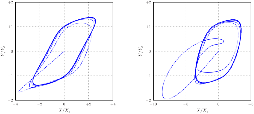
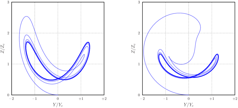
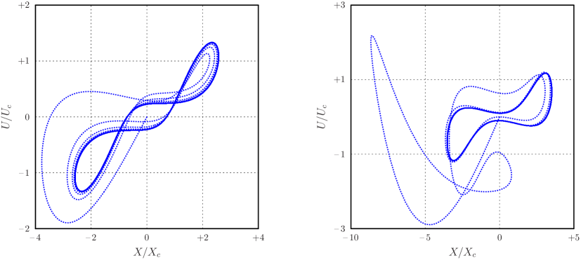
The abscissa and ordinate of Figs. 2–5 represent the taken variables rescaled with their values corresponding to the positive critical point. It can be expected that observed dynamics will become quite complicated. Under the chosen circumstances, projections on the plane are shown in Fig. 2. The instantaneous state of the system is visualized by point moving along a corresponding curve. It can be seen that the picture at the initial stage is more complicated in the second case, with a larger value of product and a larger increment. After a certain time, the clearly observed orbit attracts the current-state point of the system. The projections on the plane are shown in Fig. 3. Projections on the and planes are plotted in Fig. 4 and Fig. 5, respectively. Again, the initial stage is more complicated in the second case with a larger increment. At an initial time later, the current-state point of the system is attracted by the observed orbits. In this regard, the proposed model is similar to the standard Lorenz model and its generalizations. Of course, further properties of this model should also be addressed.
The word “butterfly” is widely used in connection with the Lorenz system [61]. It is interesting that some projections in Figs. 3–5 can also be treated to resemble a butterfly. In this sense, the new five-dimensional model (31)–(35) shares some typical features with famous examples of nonlinear dynamics. It appears that combining theoretical analysis with extensive numerical efforts is required. The above results were intended to motivate future studies of the system (31)–(35). In contrast to other modifications of the Lorenz model, the novel model has nonlinear terms in its first equation that follows from the Navier–Stokes equation. This illustrates not only what may happen in the vicinity of the point of maximum density. The proposed model can be used as a template to build similar models in cases of more practical interest, such as thermal convection in water layers near the maximum density. The above numerical results demonstrate that we have rights to expect properties similarly to those of the standard Lorenz model and its extensions. It provides a new direction for the development of models of the Lorenz type. It would also be interesting to visualize three-dimensional projections of the proposed five-dimensional model.
VI Conclusions
We have presented a novel model of thermally induced convection in the fluid inside the circle loop, similar to Tritton’s analysis. In contrast to the previous considerations, the fluid is assumed to be near the point of maximum density. This topic is interesting from its own perspective and for applications in which the temperature of maximum density is important. In Ref. [46], the experimental data on the free convection of water near its maximum density were compared with the theoretical predictions. The observed features were well reproduced by the theory presented in Ref. [45]. The above studies consider anomalous convection in a hollow cylinder with conducting lateral walls. In contrast, this work deals with the convection of fluid in the loop. A buoyancy term with the square of the excess temperature yields a five-dimensional analog of the famous Lorenz model. Unlike some known modifications of the standard Lorenz model, the proposed model has nonlinearity in the first equation. The initial interest of this author to the theme was based on temperature observations conducted in the southern basin of Lake Baikal [62, 63].
The obtained results are summarized as follows. The picture that occurs in the standard Lorenz model is, in essence, resembled. The nontrivial critical points of the system appear when the zero critical point becomes unstable. The critical value depends on the characteristics of the external temperature profile combined with the coefficient before the square of the excess temperature in the buoyancy term. The different signs at nontrivial critical points correspond to two possible directions of fluid circulation. The following facts were shown numerically. Projections on different planes in phase space are similar to those in the standard Lorenz model and its generalizations. Our findings support further studies of convective models with a nonlinear buoyancy term. They deserve more attention than they have already received. The presented model may have potential applications in the problem of free convection in fluid near its maximum density, when a linear relationship between density and temperature is not adequate. This was emphasized in the nonlinear form (2) of the thermodynamic equation of state.
Appendix A On stability of nontrivial points
For the two nontrivial critical points, one has the characteristic equation with the minus sign,
| (58) |
where . In general, the resulting quintic equation is difficult to solve analytically. For a concrete choice of the control parameters, one can calculate numerically eigenvalues of the matrix
| (59) |
Linear stability of each of the two nontrivial critical points is provided, when no eigenvalues have a strictly positive real part. In fact, the Routh–Hurwitz stability criterion can also be used here.
Let us show analytically that the two nontrivial critical points have the same eigenvalues. This physically obvious claim will serve as an additional check of the calculations. Let us consider a block matrix
| (60) |
If is invertible then (see, e.g., exercise 5.30, item (b), in the book [64])
| (61) |
We aim to use (61) with the following blocks:
The determinant is the same for both the points due to . If vanishes then it does this for both the nontrivial critical points simultaneously.
Suppose further that . Then the inverse matrix exists,
| (62) |
Elementary matrix calculations lead to the equation
| (63) |
where
| (64) |
It is clear that the resulting equation (63) is the same for both the cases .
References
- [1] P. Bergé, Y. Pomeau, and C. Vidal, Order Within Chaos: Towards a Deterministic Approach to Turbulence (Wiley, New York, 1986).
- [2] J.K. Bhattacharjee, Convection and Chaos in Fluids (World Scientific Publishing, Singapore, 1987).
- [3] C. Sparrow, The Lorenz Equations: Bifurcations, Chaos, and Strange Attractors (Springer-Verlag, New York, 1982).
- [4] T. Palmer, “Edward Norton Lorenz. 23 May 1917 — 16 April 2008,” Biogr. Mem. Fellows R. Soc. 55, 139–155 (2009)
- [5] E.N. Lorenz, “Deterministic nonperiodic flow,” J. Atmos. Sci. 20, 130–141 (1963)
- [6] E.N. Lorenz, The Essence of Chaos (University of Washington Press, Seattle, 1995).
- [7] B. Saltzman, “Finite amplitude free convection as an initial value problem — I,” J. Atmos. Sci. 19, 329–341 (1962)
- [8] J.H. Curry, “A generalized Lorenz system,” Commun. Math. Phys. 60, 193–204 (1978).
- [9] B.-W. Shen, “Nonlinear feedback in a five-dimensional Lorenz model,” J. Atmos. Sci. 71, 1701–1723 (2014).
- [10] B.-W. Shen, “Aggregated negative feedback in a generalized Lorenz model,” Int. J. Bifurc. Chaos Appl. Sci. Eng. 29, 1950037 (2019).
- [11] S. Moon, B.-S. Han, J. Park, J.M. Seo, and J.-J. Baik, “Periodicity and chaos of high-order Lorenz systems,” Int. J. Bifurc. Chaos Appl. Sci. Eng. 27, 1750176 (2017).
- [12] T. Bohr, M.H. Jensen, G. Paladin, and A. Vulpiani, Dynamical Systems Approach to Turbulence (Cambridge University Press, Cambridge, 1998).
- [13] A. Timmermann, F.-F. Jin, and J. Abshagen, “A nonlinear theory for El Niño bursting,” J. Atmos. Sci. 60, 152–165 (2003).
- [14] A. Roberts, J. Guckenheimer, E. Widiasih, A. Timmermann, and C.K.R.T. Jones, “Mixed-mode oscillations of El Niño-Southern oscillation,” J. Atmos. Sci. 73, 1755–1766 (2016).
- [15] J. Guckenheimer and R.F. Williams, “Structural stability of Lorenz attractors,” Publ. Math. IHÉS 50, 59–72 (1979).
- [16] B.-W. Shen, “On periodic solutions in the non-dissipative Lorenz model: The role of the nonlinear feedback loop,” Tellus A 70, 1471912 (2018).
- [17] F. Chillá and J. Schumacher, “New perspectives in turbulent Rayleigh–Bénard convection,” Eur. Phys. J. E 35, 58 (2012).
- [18] R.M. Lynden-Bell, S.C. Morris, J.D. Barrow, J.L. Finney, and C.L. Harper (Eds.), Water and Life: The Unique Properties of H2O (CRC Press, Boca Raton, 2010).
- [19] W.F. Vincent and C. Bertola, “Lake physics to ecosystem services: Forel and the origins of limnology,” Limnol. Oceanogr. e-Lectures 4(3), 1–47 (2014)
- [20] K. Hutter, Y. Wang, and I.P. Chubarenko, Physics of Lakes, Volume 1: Foundation of the Mathematical and Physical Background (Springer-Verlag, Berlin, 2011).
- [21] W. Grady, The Great Lakes: The Natural History of a Changing Region (Greystone Books, Vancouver, 2007).
- [22] K. Minoura (Ed.), Lake Baikal: A Mirror in Time and Space for Understanding Global Change Processes (Elsevier, Amsterdam, 2000).
- [23] R.F. Weiss, E.C. Carmack, and V.M. Koropalov, “Deep-water renewal and biological production in Lake Baikal,” Nature 349, 665–669 (1991).
- [24] D.J. Tritton, Physical Fluid Dynamics (Clarendon Press, Oxford, 1988).
- [25] E.A. Spiegel and G. Veronis, “On the Boussinesq approximation for a compressible fluid,” Astrophys. J. 131, 442–447 (1960).
- [26] J.M. Mihaljan, “A rigorous exposition of the Boussinesq approximations applicable to a thin layer of fluid,” Astrophys. J. 136, 1126–1133 (1962).
- [27] J.A. Dutton and G.H. Fichtl, “Approximate equations of motion for gases and liquids,” J. Atmos. Sci. 26, 241–254 (1969).
- [28] S. Chandrasekhar, Hydrodynamic and Hydromagnetic Stability (Clarendon Press, Oxford, 1971).
- [29] G.Z. Gershuni and E.M. Zhukhovitskii, Convective Stability of Incompressible Fluids (Keter Publishing House, Jerusalem, 1976).
- [30] F.H. Busse, “Transition to turbulence in Rayleigh–Bénard convection,” in H.L. Swinney and J.E Gollub (Eds.), Hydrodynamic Instabilities and the Transition to Turbulence, pp. 97–137 (Springer-Verlag, Berlin, 1985).
- [31] R.H. Kraichnan, “Turbulent thermal convection at arbitrary Prandtl number,” Phys. Fluids 5, 1374–1389 (1962).
- [32] J.B. McLaughlin and P.C. Martin, “Transition to turbulence in a statically stressed fluid system,” Phys. Rev. A 12, 186–203 (1975).
- [33] G. Ahlers and X. Xu, “Prandtl-number dependence of heat transport in turbulent Rayleigh–Bénard convection,” Phys. Rev. Lett. 86, 3320–3323 (2001).
- [34] K. Xia, S. Liam, and S. Zhou, “Heat-flux measurement in high-Prantdl-number turbulent Rayleigh–Bénard convection,” Phys. Rev. Lett. 88, 064501 (2002).
- [35] K.R. Sreenivasan, A. Bershadskii, and J.J. Niemela, “Mean wind and its reversal in thermal convection,” Phys. Rev. E 65, 056306 (2002).
- [36] R.C. Hwa, C.B. Yang, S. Bershadskii, J.J. Niemela, and K.R. Sreenivasan, “Critical fluctuation of wind reversals in convective turbulence,” Phys. Rev. E 72, 066308 (2005).
- [37] Q. Zhou and K.Q. Xia, “Comparative experimental study of local mixing of active and passive scalar in turbulent thermal convection,” Phys. Rev. E 77, 056312 (2008).
- [38] E. Crespo del Arco and P. Bontoux, “Numerical solution and analysis of asymmetric convention in a vertical cylinder: An effect of Prandtl number,” Phys. Fluids A 1, 1348–1359 (1989).
- [39] L. Sirovich, S. Balachandar, and M.R. Maxey, “Simulations of turbulent thermal convection,” Phys. Fluids A 1, 1911–1914 (1989).
- [40] G. Silano, K.R. Sreenivasan, and R. Verzicco, “Numerical simulations of Rayleigh–Bénard convection for Prandtl numbers between and and Rayleigh numbers between and ,” J. Fluid Mech. 662, 409–446 (2010).
- [41] N. Foroozani, J.J. Niemela, V. Armenio, and K.R. Sreenivasan, “Reorientations of the large-scale flow in turbulent convection in a cube,” Phys. Rev. E 95, 033107 (2017).
- [42] N. Foroozani, J.J. Niemela, V. Armenio, and K.R. Sreenivasan, “Turbulent convection and large scale circulation in a cube with rough horizontal surfaces,” Phys. Rev. E 99, 033116 (2019).
- [43] L.D. Landau and E.M. Lifshitz, Statistical Physics, Part 1 (Pergamon Press, Oxford, 1980).
- [44] R. Lakes, K.W. Wojciechowski, “Negative compressibility, negative Poisson’s ratio, and stability,” Phys. Stat. Sol. (b) 245, 545–551 (2008).
- [45] M. De Paz and G. Sonnino, “General theory of a convective nucleus of water in a nonsteady state and under nonlinear conditions at temperature ranges that include the density maximum,” Phys. Rev. A 39, 3031–3037 (1989).
- [46] G. Sonnino and M. De Paz, “Density profile in convection of water near C,” Phys. Rev. E 48, 1572–1575 (1993).
- [47] P. Welander, “On the oscillatory instability of a differentially heated fluid loop,” J. Fluid Mech. 29, 17–30 (1967).
- [48] C.A.J. Fletcher, Computational Galerkin Methods (Springer-Verlag, New York, 1984).
- [49] G. Veronis, “On finite amplitude instability in thermohaline convection,” J. Mar. Res. 23, 1–17 (1965).
- [50] A. Gluhovsky, “Nonlinear systems that are superpositions of gyrostats,” Sov. Phys. Dokl. 27, 823–825 (1982).
- [51] A. Gluhovsky and C. Tong, “The structure of energy conserving low-order models,” Phys. Fluids 11, 334–343 (1999).
- [52] A. Gluhovsky, C. Tong, and E. Agee, “Selection of modes in convective low-order models,” J. Atmos. Sci. 59, 1383–1393 (2002).
- [53] J.K. Bhattacharjee, K. Banerjee, D. Chowdhuri, and R. Saravanan, “Limit cycles in a forced Lorenz system,” Phys. Lett. A 104, 33–35 (1984).
- [54] G. Ahlers, P.C. Hohenberg, and M. Lücke, “Thermal convection under external modulation of the driving force. I. The Lorenz model,” Phys. Rev. A 32, 3493–3518 (1985).
- [55] O. Osenda, C.B. Briozzo, and M.O. Cáceres, “Stochastic Lorenz model for periodically driven Rayleigh–Bénard convection,” Phys. Rev. E 55, R3824–R3827 (1997).
- [56] C.W. Meyer, G. Ahlers, and D.S. Cannell, “Initial stages of pattern formation in Rayleigh–Bénard convection,” Phys. Rev. Lett. 59, 1577–1580 (1987).
- [57] M.C. Cross, “An eight-mode Lorenz model of travelling waves in binary fluid convection,” Phys. Lett. A 119, 21–24 (1986).
- [58] G. Ahlers and M. Lücke, “Some properties of an eight-mode Lorenz model for convection in binary fluids,” Phys. Rev. A 35, 470–473 (1987).
- [59] H.B. Stewart, “Visualization of the Lorenz system,” Physica D 104, 479–480 (1986).
- [60] W.H. Press, S.A. Teukolsky, W.T. Vetterling, and B.P. Flannery, Numerical Recipes: The Art of Scientific Computing (Cambridge University Press, Cambridge, 2007).
- [61] R.C. Hilborn, “Sea gulls, butterflies, and grasshoppers: A brief history of the butterfly effect in nonlinear dynamics,” Am. J. Phys. 72, 425–427 (2004)
- [62] V. Aynutdinov, A. Avrorin, V. Balkanov, et al., “Baikal neutrino telescope — An underwater laboratory for astroparticle physics and environmental studies,” Nucl. Instrum. Methods Phys. Res. A 598, 282–288 (2009).
- [63] N.M. Budnev, S.V. Lovtsov, I.A. Portyanskaya, A.E. Rastegin, and V.Yu. Rubtsov, “Analysis of hydrostatic instability based on mechanical analogy,” Russ. Phys. J. 53, 648–652 (2010).
- [64] K.M. Abadir and J.R. Magnus, Matrix Algebra (Cambridge University Press, Cambridge, 2005).