One Initialization to Rule them All: Fine-tuning via Explained Variance Adaptation

Abstract

Foundation models (FMs) are pre-trained on large-scale datasets and then fine-tuned on a downstream task for a specific application. The most successful and most commonly used fine-tuning method is to update the pre-trained weights via a low-rank adaptation (LoRA). LoRA introduces new weight matrices that are usually initialized at random with a uniform rank distribution across model weights. Recent works focus on weight-driven initialization or learning of adaptive ranks during training. Both approaches have only been investigated in isolation, resulting in slow convergence or a uniform rank distribution, in turn leading to sub-optimal performance. We propose to enhance LoRA by initializing the new weights in a data-driven manner by computing singular value decomposition on minibatches of activation vectors. Then, we initialize the LoRA matrices with the obtained right-singular vectors and re-distribute ranks among all weight matrices to explain the maximal amount of variance and continue the standard LoRA fine-tuning procedure. This results in our new method Explained Variance Adaptation (EVA). We apply EVA to a variety of fine-tuning tasks ranging from language generation and understanding to image classification and reinforcement learning. EVA exhibits faster convergence than competitors and attains the highest average score across a multitude of tasks per domain.

1 Introduction

Foundation models (Bommasani et al., 2021, FMs) are usually trained on large-scale data and then fine-tuned towards a particular downstream task. This training paradigm has led to significant advancements in the realm of language modeling (OpenAI, 2023; Touvron et al., 2023a; Reid et al., 2024), computer vision (Dehghani et al., 2023; Oquab et al., 2023), and reinforcement learning (Brohan et al., 2023; Zitkovich et al., 2023). With an increasing number of model parameters, the process of fine-tuning becomes prohibitively expensive. This results in the need for efficient alternatives to fine-tuning all parameters of the pre-trained model.

Parameter-efficient fine-tuning (PEFT) approaches are commonly used as an effective alternative to full fine-tuning (FFT). PEFT methods modify the pre-trained model by introducing a small number of new trainable parameters, while the pre-trained weights remain frozen. This leads to a substantial reduction in computational cost, both in terms of time and space. A particularly successful approach, LoRA (Hu et al., 2022), introduces new weights in the form of a low-rank decomposition for each weight matrix in the pre-trained model. After training, the new weights can be readily merged into the pre-trained weights without any additional inference latency. Recent research has explored two main avenues for enhancing LoRA: weight-driven initialization and adaptive rank allocation during training (see Table 1). While weight-driven initialization methods have shown promise, they typically rely on a uniform rank distribution across pre-trained weights. Further, they are constrained to the information stored in the pre-trained weights. Finally, existing adaptive rank allocation techniques initialize low-rank matrices randomly.

We propose a new method based on LoRA that combines adaptive rank allocation with data-driven initialization by leveraging information from the downstream task at hand. Certain activation patterns of FMs have shown to be crucial for model performance (Sun et al., 2024). Therefore, we leverage minibatches of activations computed on downstream data to initialize LoRA weights. To this end, we propagate minibatches of the fine-tuning data through the model and compute the singular value decomposition (SVD) on activation vectors to obtain the right-singular vectors. We then sort the right-singular vectors in descending order according to the variance they explain. Finally, we leverage the top-k components according to a given rank budget for initializing LoRA. This results in an effective initialization, that (i) is data-driven by leveraging information from the downstream task, and (ii) allocates ranks to pre-trained weights to maximize the explained variance throughout the model. We call the resulting method EVA, which is short for Explained Variance Adaptation. Importantly, this procedure can be performed within the first few minibatches of LoRA fine-tuning without significant computational overhead.

We demonstrate the benefits of EVA on an array of downstream tasks, namely language generation and understanding, image classification, and reinforcement learning (RL). EVA consistently improves average performance across a multitude of tasks on each domain compared to LoRA and other recently proposed initialization or rank redistribution methods. For language generation, we fine-tune 7B-9B parameter language models on math and reasoning tasks, where EVA attains the highest average performance. Further, on a set of language understanding tasks, EVA improves the average performance compared to competitors. On image classification we fine-tune a pre-trained vision transformer (Dosovitskiy et al., 2021) on a set of 19 diverse tasks. We find that EVA attains the highest average score and improves over LoRA and established extensions thereof, with most gains on in-domain data. For our RL experiments we conduct fine-tuning on continuous control tasks and find that EVA significantly exceeds performance of LoRA and even exceeds performance of full fine-tuning (FFT) when combined with DoRA (Liu et al., 2024a). Finally, we conduct ablation studies to demonstrate that the combination of direction and scale of EVA leads to the best performance.

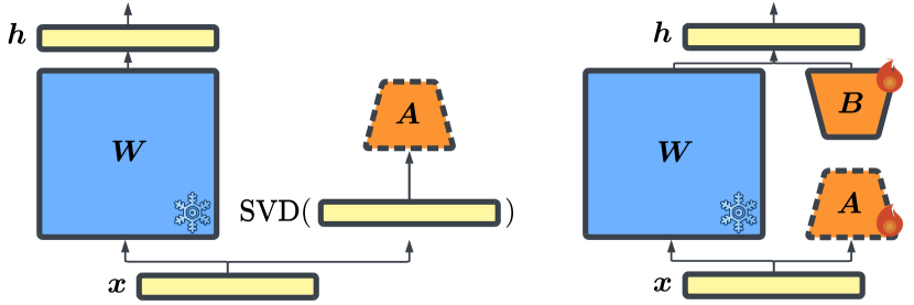
Figure 1: Left: EVA performs singular value decomposition on activation vectors for the first few minibatches to obtain a suitable initialization for the LoRA matrix $\bm{A}$. Right: After initializing $\bm{A}$, we allocate ranks to maximize the explained variance throughout the model and continue the standard LoRA fine-tuning procedure, where $\bm{W}$ is kept frozen and only $\bm{A}$ and $\bm{B}$ are trained.

Table 1: Comparison of EVA to existing initialization schemes for LoRA. Existing works either focus on weight-driven initialization or adaptive rank allocation. EVA combines data-driven initialization with adaptive rank allocation to enhance convergence and downstream performance.

Method	Initialization	Adaptive ranks
LoRA (Hu et al., 2022)	Random	✗
AdaLoRA (Zhang et al., 2023a)	Random	✓
PiSSA (Meng et al., 2024)	Weight-driven	✗
OLoRA (Büyükakyüz, 2024)	Weight-driven	✗
EVA (Ours)	Data-driven	✓

2 Related Work

LoRA (Hu et al., 2022) has sparked widespread interest in leveraging low-rank decompositions for fine-tuning due to its simplicity. Building on the success of LoRA, a number of other variants have been proposed (Kopiczko et al., 2024; Zi et al., 2023; Babakniya et al., 2023; Dettmers et al., 2023; Li et al., 2023; Nikdan et al., 2024; Liu et al., 2024a; Zhang et al., 2023a; Hayou et al., 2024b; Chavan et al., 2023). The most similar variants to EVA are AdaLoRA (Zhang et al., 2023a) and PiSSA (Meng et al., 2024). AdaLoRA adaptively alters the number of ranks for LoRA matrices during fine-tuning. Other more recent approaches learn gates to switch ranks on or off during fine-tuning (Liu et al., 2024b; Meo et al., 2024). In contrast, the data-driven initialization allows EVA to redistribute ranks for each LoRA matrix prior to fine-tuning by leveraging a small number of minibatches of data. PiSSA initializes LoRA matrix $\bm{A}$ via the top singular vectors of the pre-trained weight matrices. Contrary, EVA initializes $\bm{A}$ via the right-singular vectors of minibatches of activation vectors and is therefore data-driven. Since EVA mostly constitutes an effective initialization, it can be readily plugged into other LoRA variants such as DoRA (Liu et al., 2024a).

Initialization of LoRA matrices Common initialization schemes for neural networks (He et al., 2015; Glorot & Bengio, 2010) were designed to stabilize training of deep neural networks based on activation functions and depth. In the context of PEFT, Hu et al. (2022) and Liu et al. (2022) explored data-driven initialization by either pre-training on a different task first, or by unsupervised pre-training on the task at hand. Contrary, EVA does not require any gradient update steps, therefore it is much more efficient. Similarly, Nikdan et al. (2024) utilize a warm-up stage in LoRA fine-tuning, where gradients with respect to LoRA weights are used to initialize a sparse matrix for sparse adaptation (Sung et al., 2021) in combination with LoRA. Alternatively, Babakniya et al. (2023) initialize LoRA matrices using SVD on weight matrices obtained after a few steps of full fine-tuning for federated learning with heterogeneous data. Meng et al. (2024) use the main directions of the pre-trained weights to initialize the LoRA matrices. In contrast, EVA takes a data-driven approach to initialize the LoRA matrices, instead of relying on components of the pre-trained weights. Similar initialization schemes were proposed by Mishkin & Matas (2016); Krähenbühl et al. (2016) for training deep networks from scratch.

Increasing efficiency of LoRA Several works have investigated how to further break down the complexity of LoRA for fine-tuning FMs. Kopiczko et al. (2024) decrease the memory complexity of LoRA by initializing both $\bm{A}$ and $\bm{B}$ at random and keeping them frozen while merely training newly-introduced scaling vectors. This way, only random seeds for initializing $\bm{A}$ and $\bm{B}$ need to be stored. Another fruitful avenue is quantization (Dettmers et al., 2022), which has been successfully combined with LoRA fine-tuning (Dettmers et al., 2023). Other LoRA variants (Nikdan et al., 2024; Valipour et al., 2023; Meng et al., 2024) also provide quantized versions. It has also been shown that proper initialization for quantization results in improved fine-tuning performance (Li et al., 2023).

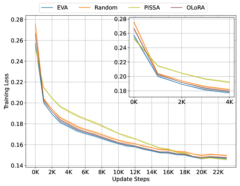
Figure 2: Left: Training loss for fine-tuning Llama-3.1-8B on the MetaMathQA dataset. We compare EVA to recently proposed initialization methods OLoRA, PiSSA, and random initialization (LoRA). We show mean and standard deviation across three random seeds. Right: Mean and standard deviation of gradient norm for EVA, PiSSA, OLoRA and Random initialization of LoRA matrices. EVA exhibits significantly larger gradient norm leading to faster convergence.

3 Method

EVA aims at initializing LoRA weights in a data-driven manner by leveraging data from the downstream task. Since EVAbuilds on low-rank decomposition of weight matrices as in LoRA (Hu et al., 2022), we first briefly explain LoRA in Section 3.1. In Section 3.2, we describe how we obtain an effective initialization for the low-rank decomposition of LoRA matrices via SVD on activation vectors. This enables an adaptive assignment of ranks across all layers to maximize the explained variance throughout the pre-trained model We explain this in more detail in Section 3.3.

3.1 Low-Rank Adaptation (LoRA)

LoRA adds new trainable weights which are computed via an outer product of low-rank matrices (Hu et al., 2022). This is motivated by the low intrinsic dimensionality of language models (Aghajanyan et al., 2021) and relies on the assumption that the gradients during fine-tuning are also of low rank (Gur-Ari et al., 2018; Zhang et al., 2023b; Gauch et al., 2022). In the following, we explain LoRA in more detail. Let $\bm{x}\in\mathbb{R}^{d\times 1}$ be the input to a pre-trained weight matrix $\bm{W}\in\mathbb{R}^{k\times d}$. Then, LoRA introduces new weight matrices $\bm{A}$ and $\bm{B}$ as a low-rank decomposition

$$\bm{h}=\bm{W}\bm{x}+\bm{B}\bm{A}\bm{x}\,,$$ (1)

where $\bm{B}\in\mathbb{R}^{k\times r}$ and $\bm{A}\in\mathbb{R}^{r\times d}$. The rank $r$ is a hyperparameter with $r\ll k$. During fine-tuning, $\bm{W}$ remains frozen and only $\bm{A}$ and $\bm{B}$ are updated. Usually $\bm{B}$ is initialized with zeros, such that fine-tuning starts from the pre-trained model. $\bm{A}$ is usually initialized at random. Additionally, Hu et al. (2022) introduce a hyperparamter $\alpha$ which is used to scale $\bm{B}\bm{A}\bm{x}$ by $\frac{\alpha}{r}$.

3.2 Data-driven Initialization of Low-Rank Adaptation

Our aim is to find an effective initialization for the low-rank matrix $\bm{A}$ in a data-driven manner to maximize performance on the downstream task. To this end, we perform SVD on batches of activation vectors $\bm{X}\in\mathbb{R}^{b\times d}$ to obtain the right-singular values, which constitute the directions that capture most of the variance. This procedure is done during the initial training stage where we propagate minibatches of data through the model and incrementally update the right-singular vectors. More formally, we collect batches of activations $\bm{X}^{i}$ for $N$ pre-trained weight matrices $\bm{W}^{i}\in\{\bm{W}^{0},\bm{W}^{1},...,\bm{W}^{N}\}$ that we choose to update fine-tune. Subsequently, we compute the SVD on each $\bm{X}^{i}$ to obtain the right-singular vectors $\bm{v}^{i}_{j,:}$ and respective singular values $\sigma^{i}_{j}$ as

$$\bm{X}^{i}=\sum_{j=1}^{r}\bm{u}^{i}_{:,j}\sigma^{i}_{j}\bm{v}^{i}_{j,:}.$$ (2)

Importantly, we compute the SVD incrementally on each minibatch of fine-tuning data and update $\bm{v}^{i}_{:r,:}$ after each forward pass through the model. After each step we check whether $\bm{v}^{i}_{:r,:}$ has converged. To this end, we measure the column-wise cosine similarity between subsequent computations of $\bm{v}_{:r,:}$ and determine convergence based on a threshold $\tau$. If the right-singular values have converged, i.e. $\operatorname{cossim}(\bm{v}_{j,:}^{i,t-1},\bm{v}_{j,:}^{i,t})\geq\tau\quad\forall\quad 1\leqslant j\leqslant r$, we initialize $\bm{A}^{i}=\bm{v}^{i}_{:r,:}$ and exclude the corresponding weight matrix from subsequent SVD computations. We continue this procedure until all $\bm{v}_{:r,:}^{i}$ have converged.

The computation of SVD introduces computational overhead in the initial training stage. Since we do not require gradient computation or storing of optimizer states, there is no overhead in terms of memory. SVD has a time complexity of $\mathcal{O}(\operatorname{min}(b^{2}d,bd^{2}))$ which can be reduced to $\mathcal{O}(k^{2}b)$ for $k<<d$ by randomly choosing $k$ columns from $\bm{X}$ as introduced in Halko et al. (2011). Let $T$ be the number of minibatches until all components are converged for $N$ weight matrices, then the time complexity is $\mathcal{O}(NTk^{2}b)$. In other words, the complexity scales linearly with the number of weight matrices and the number of minibatches. To speed up the computation of SVD, we provide an implementation that runs entirely on GPU.

3.3 Adaptive Rank Allocation

The singular values obtained by SVD provide an estimate of the variance that is explained by their components. Leveraging this information, we can redistribute ranks across weight matrices of the pre-trained model such that the maximum amount of variance is explained. This can be done by allocating more ranks to layers that propagate more information, i.e., explain more variance. More formally, the variance explained by each component in $\bm{v}^{i}_{j,:}$ is given by their explained variance ratio

$$\xi^{i}_{j}=\frac{\sigma^{i^{2}}_{j}}{(M-1)||\bm{\sigma}^{i}||_{1}},$$ (3)

where $||\cdot||_{1}$ denotes the $\ell_{1}$ norm, $\bm{\sigma}^{i}$ is a vector containing all $r$ singular values, and $M$ is the total number of samples used for the incremental SVD computation. Next, we sort the components $\bm{v}^{i}_{j,:}$ for each weight matrix in descending order according to their explained variance ratio $\xi^{i}_{j}$. Finally, we assign ranks to pre-traiend weights until we reach a certain rank budget.

Algorithm 1 Fine-tuning via EVA

0:  FM $\psi(\cdot)$, $\rho$, rank $r$, dataset $\mathcal{D}$

1:  while $\texttt{not}\,\,\texttt{all\_converged}(\psi)$ do

2:     $\bm{X}\leftarrow\psi(\texttt{next}(\mathcal{D}))$ $\triangleright$ get activations

3:     $\bm{V}_{\text{new}},\bm{\xi}\leftarrow\operatorname{SVD}(\bm{X},\rho r)$

4:     if $\texttt{isclose}(\bm{V}_{\text{old}},\bm{v}_{\text{new}})$ then

5:        $\texttt{wrap\_and\_initialize}(\bm{W}_{j},\bm{V}_{\text{new}})$

6:     end if

7:     $\bm{V}_{old}\leftarrow\bm{V}_{new}$

8:  end while

9:  $\texttt{redistribute\_ranks}(\psi,\bm{\xi},\bm{V}_{\text{new}})$

10:  $\texttt{lora\_finetune}(\psi,\bm{X})$

Additionally, we introduce a hyperparameter $\rho\in[1,\infty)$ which controls the uniformity of the rank distribution. $\rho$ determines the number of ranks that we compute during SVD and increasing $\rho$ allows for an increasingly heterogeneous rank distribution. That is, for each $\bm{W}^{i}$ we compute $r\rho$ components initially meaning we obtain ${N}{r}\rho$ components in total. For the redistribution we only use the top ${N}{r}$ components according to their explained variance ratio $\xi^{i}_{j}$. Thus, setting $\rho=1$, results in a uniform rank distribution as in LoRA, but initialized according to EVA. Therefore, $\rho$ provides us with the means to change the rank distribution in a controlled manner prior to fine-tuning at the initialization stage, as opposed to learning it throughout the training process as done in prior works (Zhang et al., 2023a; Valipour et al., 2023; Meo et al., 2024). In practice we found that the redistribution converges for values of $\rho>2$ (see Appendix G). Finally, we initialize $\bm{B}$ with zeros and perform the standard LoRA fine-tuning, as recommended in Hayou et al. (2024a). In Algorithm 1 we provide pseudocode for EVA.

4 Experiments

First, we elaborate on implementation details of EVA in Section 4.1. Then, we show results for fine-tuning large language models (LLMs) on math and reasoning tasks in Section 4.2 and language understanding tasks in Section 4.3. Further we show results for image classification in Section 4.4 and decision making tasks in Section 4.5. Finally, in Section 4.6 we demonstrate that the computational overhead induced by EVA over LoRA is negligible and that incremental SVD converges and is invariant to batch order and batch size.

Table 2: Comparison of LoRA and DoRA to different initialization and rank re-distribution methods on NLG tasks. We report average performance across three seeds and respective standard deviation in Table 11. EVA+DoRA and EVA consistently attain the highest average performance across all tasks.

Model	Method	BoolQ	PIQA	SIQA	HellaSwag	Winogrande	ARC-e	ARC-c	OBQA	Avg.
Llama-2-7B	LoRA	67.2	83.9	82.0	94.7	84.0	87.8	74.1	84.0	82.2
	AdaLoRA	74.8	82.2	80.5	93.3	79.4	86.1	71.1	80.6	81.0
	PiSSA	62.6	84.8	81.2	94.5	84.8	87.8	74.8	85.4	82.0
	OLoRA	68.7	84.8	82.2	95.0	85.0	88.1	74.9	85.2	82.9
	EVA	71.2	85.2	82.1	95.2	84.5	88.9	75.6	85.0	83.4
	DoRA	68.3	85.1	82.2	94.9	84.3	88.7	74.8	86.3	83.1
	EVA+DoRA	73.5	85.3	82.4	95.2	84.8	88.9	76.0	87.3	84.2
Llama-3.1-8B	LoRA	85.7	90.3	83.0	96.9	88.4	94.2	84.8	90.1	89.2
	AdaLoRA	83.9	89.5	81.7	96.2	86.3	93.7	82.7	86.8	87.6
	PiSSA	72.9	87.3	81.6	95.3	87.8	91.7	81.2	87.6	85.7
	OLoRA	86.0	90.4	83.9	97.0	88.6	94.5	84.7	90.3	89.4
	EVA	85.5	90.8	83.3	97.1	88.6	94.7	85.7	89.5	89.4
	DoRA	86.2	90.8	83.4	96.9	88.6	94.3	84.9	89.4	89.3
	EVA+DoRA	85.8	90.8	83.9	97.1	89.2	94.4	85.9	90.5	89.7
Gemma-2-9B	LoRA	88.3	92.9	85.2	97.8	92.3	97.2	89.9	94.4	92.2
	AdaLoRA	87.3	91.8	84.6	97.3	91.3	97.0	90.0	92.6	91.5
	PiSSA	81.4	90.0	82.5	95.5	89.0	93.6	83.5	90.8	88.3
	OLoRA	87.7	92.5	85.2	97.5	92.5	96.6	88.7	93.7	91.8
	EVA	88.6	93.0	85.3	97.9	92.8	97.5	90.5	94.5	92.5
	DoRA	88.3	92.6	84.9	97.7	92.2	97.1	89.9	94.5	92.1
	EVA+DoRA	88.6	93.1	85.1	97.9	92.5	97.3	89.6	94.8	92.4

4.1 Implementation Details

We follow the standard LoRA training procedure from Hu et al. (2022). Similar to Kalajdzievski (2023), we found LoRA training to be very sensitive to the scaling parameter $\alpha$. Therefore, we set $\alpha=1$ since we found this to be the most stable setting and additionally tune the learning rate. We apply EVA to pre-trained weights only, i.e., we do not initialize newly introduced classifier heads. Following Zhang et al. (2023a), we apply LoRA to all pre-trained weight matrices except for the embedding layer. For EVA we always search over $\rho\in\{1,2\}$ to cover both uniform and non-uniform rank allocation and report the best score. All models we used are publicly available on the huggingface hub (Wolf et al., 2020). For the implementation of baselines we leverage the widely used PEFT library (Mangrulkar et al., 2022). Across experiments we highlight the highest scores in boldface and underline the second-highest.

Table 3: Comparison of EVA to other initialization and adaptive rank methods on GSM8K and MATH datasets. We report mean and standard deviation across three random seeds.

Model	Method	GSM8K	MATH
Llama-2-7B	LoRA	$\text{59.7}_{\pm.8}$	$\text{10.9}_{\pm.2}$
	AdaLoRA	$\text{56.9}_{\pm.4}$	$\text{9.6}_{\pm.2}$
	PiSSA	$\text{61.1}_{\pm.3}$	$\text{12.6}_{\pm.4}$
	OLoRA	$\text{60.7}_{\pm.5}$	$\text{11.8}_{\pm.3}$
	EVA	$\text{61.9}_{\pm.5}$	$\text{13.1}_{\pm.3}$
	DoRA	$\text{59.8}_{\pm.5}$	$\text{11.5}_{\pm.2}$
	EVA+DoRA	$\text{{62.5}}_{\pm.8}$	$\text{{13.4}}_{\pm.01}$
Llama-3.1-8B	LoRA	$\text{78.3}_{\pm.6}$	$\text{30.1}_{\pm.5}$
	AdaLoRA	$\text{76.9}_{\pm.2}$	$\text{28.9}_{\pm.7}$
	PiSSA	$\text{78.8}_{\pm.2}$	$\text{29.5}_{\pm.5}$
	OLoRA	$\text{78.0}_{\pm.1}$	$\text{31.0}_{\pm.7}$
	EVA	$\text{78.8}_{\pm.3}$	$\text{{31.2}}_{\pm.3}$
	DoRA	$\text{77.9}_{\pm.1}$	$\text{30.2}_{\pm.5}$
	EVA+DoRA	$\text{{79.1}}_{\pm.5}$	$\text{30.8}_{\pm.4}$
Gemma-2-9B	LoRA	$\text{83.4}_{\pm.9}$	$\text{40.7}_{\pm.2}$
	AdaLoRA	$\underline{\text{83.5}}_{\pm.5}$	$\text{41.1}_{\pm.4}$
	PiSSA	$\text{79.8}_{\pm.5}$	$\text{34.9}_{\pm.2}$
	OLoRA	$\text{82.2}_{\pm.2}$	$\text{39.4}_{\pm.6}$
	EVA	$\text{{83.6}}_{\pm.8}$	$\text{{41.5}}_{\pm.3}$
	DoRA	$\text{82.5}_{\pm.6}$	$\text{39.7}_{\pm.4}$
	EVA+DoRA	$\text{82.9}_{\pm.3}$	$\text{40.0}_{\pm.6}$

4.2 Language Generation

We fine-tune three different LLMs, namely Llama-2-7B (Touvron et al., 2023b), Llama-3.1-8B (Dubey et al., 2024), and Gemma-2-9B (Rivière et al., 2024) on common sense and math reasoning benchmarks. For common sense reasoning we follow Liu et al. (2024a) and amalgamate a training set consisting of BoolQ (Christopher et al., 2019), PIQA (Bisk et al., 2020), SIQA (Sap et al., 2019), HellaSwag (Zellers et al., 2019), Winogrande (Sakaguchi et al., 2020), ARC-e and ARC-c (Clark et al., 2018) and OpenBookQA (Mihaylov et al., 2018). We apply all methods listed in Table 1 to all three models and additionally add a comparison to DoRA (Liu et al., 2024a) and EVA+DoRA, which combines EVA with DoRA. We train all methods with rank $r=16$ and a learning rate of $5\text{e}-4$ for three random seeds. Further details on the fine-tuning settings can be found in Appendix B. We present our results in Table 2. For Llama-2-7B and Llama-3.1-8B EVA+DoRA ($\rho=1$) is the best performing method on average while also exhibiting the best individual scores on most tasks. For Gemma-2-9B, EVA with adaptive ranks ($\rho=2$) yields the highest performance. EVA as well as EVA+DoRA are consistently among the best performing methods on all individual tasks. This highlights the effectiveness of EVA’s data-driven initialization and rank allocation.

For the math fine-tuning experiments, we fine-tune all models on the MetaMathQA dataset (Yu et al., 2024) for one epoch with the same hyperparameters that we used for the common sense reasoning benchmarks and report the results in Table 3. We observe that EVA attains the highest performance on the GSM8K dataset for Gemma-2-9B using $\rho=2$. For Llama-2-7B and Llama-3.1-8B the best performing method is EVA+DoRA using $\rho=1$ closely followed by EVA. On MATH, EVA+DoRA performs best for Llama-2-7B with $\rho=1$, while EVA attains the highest score for Llama-3.1-8B with $\rho=1$ and Gemma-2-9B with $\rho=2$. These results indicates that the performance of adaptive rank allocation depends on the selected model. We further analyze the resulting rank distributions for different values of $\rho$ for Llama-2-7B and their effect on downstream performance in Appendix G. Finally, we provide additional results for Llama-2-7B on code fine-tuning tasks in Appendix B.

4.3 Language Understanding

We train $\text{RoBERTa}_{\text{Large}}$ (Liu et al., 2019) and $\text{DeBERTav3}_{\text{Base}}$ (He et al., 2023) on the GLUE benchmark (Wang et al., 2019). The GLUE benchmark comprises eight downstream tasks, such as natural language inference, or sentiment analysis. Additionally to learning rate, we also search over different ranks within a maximal rank budget ($r=16$). For further details about datasets, implementation, or hyperparameters, we refer the reader to Appendix C. We also add FFT as a baseline, but neglect EVA+DoRA due to time constraints and report Matthew’s correlation for CoLA, Pearson correlation for STS-B, and accuracy for the remaining tasks in Table 4.

Table 4: Comparison of all methods for $\text{RoBERTa}_{\text{Large}}$ (top) and $\text{DeBERTav3}_{\text{Base}}$ (bottom) on GLUE tasks. We report mean and standard deviation of Matthew’s correlation for CoLA, Pearson correlation for STS-B, matched accuracy for MNLI, and accuracy for remaining tasks. For CoLA, RTE, MRPC, and STS-B we average over five seeds and for the remaining tasks over three seeds.

Method	MNLI	QNLI	QQP	SST2	CoLA	MRPC	RTE	STS-B	Avg
FFT	$90.2$	$94.7$	$\bm{92.2}$	$\bm{96.4}$	$68.0$	$90.9$	$86.6$	$92.4$	$88.93$
LoRA	$90.7_{\pm.1}$	$\underline{94.8}_{\pm.1}$	$92.0_{\pm.0}$	$96.2_{\pm.3}$	$69.1_{\pm.5}$	$\underline{91.1}_{\pm.6}$	$88.1_{\pm 1.1}$	$92.3_{\pm.1}$	$89.29$
AdaLoRA	$90.5_{\pm.1}$	$\underline{94.8}_{\pm.2}$	$90.6_{\pm.1}$	$96.1_{\pm.2}$	$68.2_{\pm.7}$	$90.7_{\pm.6}$	$84.4_{\pm.9}$	$91.8_{\pm.1}$	$88.39$
PiSSA	$90.1_{\pm.1}$	$94.7_{\pm.0}$	$91.0_{\pm.0}$	$96.1_{\pm.2}$	$68.7_{\pm 1.3}$	$90.4_{\pm.6}$	$87.6_{\pm.5}$	$\underline{92.5}_{\pm.3}$	$88.89$
OLoRA	$\bm{90.9_{\pm.1}}$	$\bm{95.0_{\pm.1}}$	$92.0_{\pm.2}$	$\underline{96.3}_{\pm.3}$	$69.0_{\pm 1.5}$	$91.0_{\pm 1.0}$	$87.9_{\pm 1.2}$	$92.4_{\pm.1}$	$89.32$
EVA	$\underline{90.8}_{\pm.1}$	$\bm{95.0_{\pm.2}}$	$\underline{92.1}_{\pm.1}$	$96.2_{\pm.1}$	$\bm{69.5_{\pm 1.4}}$	$\bm{91.4_{\pm.8}}$	$\bm{88.8_{\pm 1.2}}$	$\bm{92.6_{\pm.1}}$	$\bm{89.55}$
DoRA	$89.5_{\pm.1}$	$94.6_{\pm.1}$	$89.9_{\pm.1}$	$96.1_{\pm.1}$	$\underline{69.3}_{\pm.8}$	$91.0_{\pm.6}$	$\underline{88.4}_{\pm 1.2}$	$92.4_{\pm.1}$	$88.90$
FFT	$90.1$	$94.0$	$\underline{92.4}$	$95.6$	$69.2$	$89.5$	$83.8$	$91.6$	$88.28$
LoRA	$90.5_{\pm.1}$	$94.3_{\pm.1}$	$\underline{92.4}_{\pm.1}$	$\underline{95.2}_{\pm.3}$	$72.0_{\pm 1.3}$	$91.4_{\pm.7}$	$88.9_{\pm.5}$	$91.7_{\pm.1}$	$89.64$
AdaLoRA	$\bm{90.8}$	$\bm{94.6}$	$92.2$	$96.1$	$71.5$	$90.7$	$88.1$	$\underline{91.8}$	$89.46$
PiSSA	$90.1_{\pm.3}$	$94.1_{\pm.1}$	$91.8_{\pm.1}$	$95.8_{\pm.1}$	$\bm{72.7}_{\pm 1.7}$	$90.9_{\pm.6}$	$86.5_{\pm 1.2}$	$91.6_{\pm.2}$	$89.19$
OLoRA	$90.5_{\pm.1}$	$\underline{94.4}_{\pm.1}$	$\bm{92.6}_{\pm.1}$	$\bm{96.2}_{\pm.2}$	$72.0_{\pm 1.0}$	$91.6_{\pm.7}$	$\underline{89.1}_{\pm.9}$	$\bm{92.0}_{\pm.2}$	$\underline{89.80}$
EVA	$\underline{90.6}_{\pm.1}$	$\underline{94.4}_{\pm.1}$	$\underline{92.4}_{\pm.04}$	$\bm{96.2}_{\pm.2}$	$\underline{72.5}_{\pm 1.3}$	$\underline{91.8}_{\pm.6}$	$\bm{89.4}_{\pm.7}$	$\bm{92.0_{\pm.2}}$	$\bm{89.91}$
DoRA	$89.0_{\pm.2}$	$94.1_{\pm.1}$	$88.0_{\pm.1}$	$94.6_{\pm.4}$	$70.3_{\pm.5}$	$\bm{91.9}_{\pm.6}$	$87.8_{\pm.7}$	$\underline{91.8}_{\pm.1}$	$88.44$

For $\text{RoBERTa}_{\text{Large}}$, EVA attains the highest scores on QNLI, CoLA, MRPC, RTE, and STS-B, leading to the highest average score. Interestingly, DoRA usually only slightly improves over LoRA on low resource tasks (RTE, MRPC), while performing worse in high resource tasks (MNLI, QNLI, QQP, SST2). We also compare LoRA to EVA in Table 14 in Appendix C for different rank budgets, where EVA consistently improves over LoRA. For $\text{DeBERTav3}_{\text{Base}}$, EVA reaches the highest scores on SST2, RTE, and STS-B, again leading to the highest average score across all tasks. We visualize resulting rank distribution patterns of EVA for different GLUE tasks in Appendix C. More ranks are assigned to higher layers of the query, key, and value projections in the self-attention, while the remaining weights often receive a lower number of ranks. This is a consistent pattern for both, $\text{DeBERTav3}_{\text{Base}}$ and $\text{RoBERTa}_{\text{Large}}$.

Table 5: Fine-tuning DINOv2-g/14 on the VTAB-1K benchmark. Best average performance is highlighted in boldface. We report average accuracy across five seeds.

	Natural							Specialized				Structured
	Cifar100	Caltech101	DTD	Flower102	Pets	SVHN	Sun397	Camelyon	EuroSAT	Resisc45	Retinopathy	Clevr-Count	Clevr-Dist	DMLab	KITTI-Dist	dSpr-Loc	dSpr-Ori	sNORB-Azim	sNORB-Ele	Average
FFT	73.1	89.7	78.4	99.7	92.2	89.5	55.5	74.8	95.0	88.2	70.5	93.6	64.2	63.6	68.8	92.0	64.3	50.2	56.8	76.8
LoRA	85.9	92.2	82.2	99.7	94.5	64.1	63.6	88.8	97.0	92.6	76.6	97.7	65.3	62.1	83.6	90.6	63.0	37.1	52.3	78.4
AdaLoRA	85.4	92.5	81.4	99.7	95.2	90.5	62.2	87.1	96.4	91.2	76.6	94.4	64.4	60.3	83.7	85.4	61.0	32.9	46.0	78.2
PiSSA	85.5	93.6	82.3	99.7	94.6	92.8	62.3	87.1	96.6	91.9	76.3	95.0	66.3	63.2	84.9	90.5	60.1	36.3	48.6	79.4
OLoRA	85.5	93.0	82.1	99.7	95.1	78.3	62.1	86.7	96.3	91.9	76.8	94.3	66.0	62.4	71.3	89.0	60.9	34.3	49.5	77.6
EVA	85.6	93.9	82.2	99.7	95.9	93.2	63.6	86.8	96.6	92.3	76.1	96.1	65.1	61.1	83.3	91.4	61.6	35.0	55.0	79.7
DoRA	85.9	92.7	82.1	99.7	95.2	34.4	61.4	88.6	96.8	92.4	76.8	97.6	65.4	62.7	84.4	43.2	63.1	37.8	52.6	74.4
EVA+DoRA	86.2	92.1	81.9	99.7	94.9	93.8	62.4	88.3	96.6	92.6	76.7	97.2	65.5	54.1	83.7	93.3	62.3	37.5	54.5	79.6

4.4 Image Classification

We investigate the efficacy of EVA on the VTAB-1K (Zhai et al., 2019) benchmark, which has been widely used to evaluate PEFT methods. VTAB-1K comprises 19 image classification tasks that are divided into natural images, specialized images (medical images and remote sensing), and structured images (e.g. orientation prediction, depth estimation or object counting). We fine-tune a DINOv2-g/14 model (Oquab et al., 2023) that consists of around 1.1B parameters. For implementation details or hyperparameters we refer the reader to Appendix D. Our results are shown in Table 5 and we additionally report error bars in Table 17. EVA and EVA+DoRA attain the best and second-best average accuracy across all tasks, respectively. Interestingly, EVA mainly improves over competitors on the natural tasks, i.e. in-domain datasets. LoRA performs best on the specialized tasks and full fine-tuning (FFT) performs best on the structured task. However, both LoRA and FFT perform worse on the remaining tasks, leading to a worse average score compared to EVA and EVA+DoRA.

4.5 Decision Making

We follow the single task fine-tuning experiments in Schmied et al. (2023) and fine-tune a Decision Transformer (Chen et al., 2021a, DT) on the Meta-World benchmark suite (Yu et al., 2020). Meta-World consists of a diverse set of 50 tasks for robotic manipulation, such as object manipulation, grasping, or pushing buttons. We split Meta-World according to Wolczyk et al. (2021) into 40 pre-training tasks (MT40) and 10 fine-tuning tasks (CW10). We pre-train a 12 M parameter DT on MT40 and fine-tune it on the CW10 holdout tasks.

Table 6: Results for single task fine-tuning experiments on the Meta-World benchmark. We report mean success rates and standard error across three seeds for every task.

	faucet-close	hammer	handle-press	peg-unplug	push-back	push	push-wall	shelf-place	stick-pull	window-close	Average
FFT	$1.0_{\pm.0}$	$\underline{0.97}_{\pm.03}$	$1.0_{\pm.0}$	$\underline{0.77}_{\pm.05}$	$\underline{0.87}_{\pm.05}$	$\bm{1.0}_{\pm.0}$	$\bm{1.0}_{\pm.0}$	$1.0_{\pm.0}$	$\underline{0.63}_{\pm.03}$	$1.0_{\pm.0}$	$0.92$
LoRA	$1.0_{\pm.0}$	$\bm{1.0}_{\pm.0}$	$1.0_{\pm.0}$	$0.6_{\pm.05}$	$0.63_{\pm.1}$	$\bm{1.0}_{\pm.0}$	$\bm{1.0}_{\pm.0}$	$1.0_{\pm.0}$	$0.4_{\pm.09}$	$1.0_{\pm.0}$	$0.86$
AdaLoRA	$1.0_{\pm.0}$	$\underline{0.97}_{\pm.03}$	$1.0_{\pm.0}$	$0.4_{\pm.09}$	$0.57_{\pm.1}$	$\underline{0.97}_{\pm.03}$	$\underline{0.97}_{\pm.03}$	$1.0_{\pm.0}$	$0.13_{\pm.07}$	$1.0_{\pm.0}$	$0.80$
PiSSA	$1.0_{\pm.0}$	$\bm{1.0}_{\pm.0}$	$1.0_{\pm.0}$	$0.43_{\pm 0.11}$	$0.57_{\pm 0.03}$	$\bm{1.0}_{\pm.0}$	$\bm{1.0}_{\pm.0}$	$1.0_{\pm.0}$	$0.53_{\pm 0.1}$	$1.0_{\pm.0}$	$0.85$
OLoRA	$1.0_{\pm.0}$	$\underline{0.97}_{\pm 0.03}$	$1.0_{\pm.0}$	$0.57_{\pm 0.1}$	$0.63_{\pm 0.03}$	$\bm{1.0}_{\pm.0}$	$\bm{1.0}_{\pm.0}$	$1.0_{\pm.0}$	$0.6_{\pm 0.12}$	$1.0_{\pm.0}$	$0.88$
EVA	$1.0_{\pm.0}$	$\underline{0.97}_{\pm.03}$	$1.0_{\pm.0}$	$0.63_{\pm.03}$	$0.77_{\pm.05}$	$\bm{1.0}_{\pm.0}$	$\bm{1.0}_{\pm.0}$	$1.0_{\pm.0}$	$\underline{0.63}_{\pm.07}$	$1.0_{\pm.0}$	$0.90$
DoRA	$1.0_{\pm.0}$	$\bm{1.0}_{\pm.0}$	$1.0_{\pm.0}$	$0.6_{\pm 1.2}$	$\bm{1.0}_{\pm.0}$	$\bm{1.0}_{\pm.0}$	$\bm{1.0}_{\pm.0}$	$1.0_{\pm.0}$	$\bm{0.67_{\pm 1.5}}$	$1.0_{\pm.0}$	$\underline{0.93}$
EVA+DoRA	$1.0_{\pm.0}$	$\bm{1.0}_{\pm.0}$	$1.0_{\pm.0}$	$\bm{0.8_{\pm.08}}$	$\bm{1.0}_{\pm.0}$	$\bm{1.0}_{\pm.0}$	$\bm{1.0}_{\pm.0}$	$1.0_{\pm.0}$	$\underline{0.63}_{\pm.03}$	$1.0_{\pm.0}$	$\bm{0.94}$

We report success rates and standard errors for each task of CW10 in Table 6. We observe that EVA significantly reduces that gap between LoRA and FFT. Furthermore, DoRA performs particularly well in this experiment and exceeds FFT performance. Finally, our EVA+DoRA even improves upon DoRA and attains the best average performance across all tasks. We report results for different rank budgets in Table 19, as well as implementation details and hyperparameters in Appendix E.

4.6 SVD Convergence Analysis

The data-driven initialization of EVA relies on incremental SVD on minibatches of activations in the initial training stage. In Figure 3, left, we show that this process converges for Llama-2-7B on MetaMathQA for different minibatch sizes. Using a minibatch size of 4 the computation for EVA’s initialization lasts for approximately 80 seconds, which corresponds to around 90 minibatches. For a batch size of 32 the computation of the SVD components takes around 500 seconds. In Figure 3, right, we additionally show, that the main components obtained via SVD mostly remain consistent across different batch orders for a batch size of 4, again for Llama-2-7B on MetaMathQA. To this end, we plot cosine similarity between components obtained via incremental SVD after rank redistribution. These results indicate that these models exhibit certain activation patterns that remain consistent across different batch orders which lead to a robust initialization for EVA. We also show that the components for different batch sizes converge to mostly the same final initialization in Appendix F.

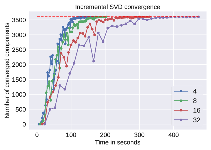
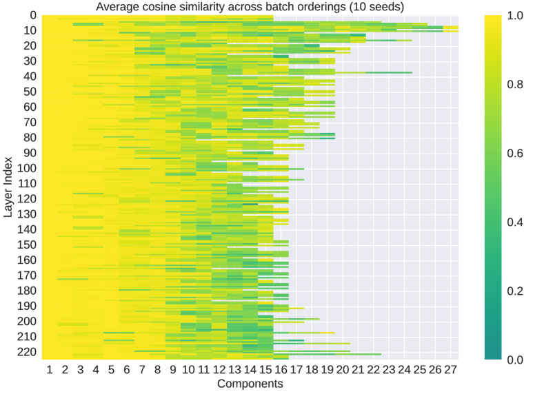
Figure 3: Left: Time in seconds until convergence of incremental SVD components for different batch sizes for Llama-2-7B on the MetaMathQA dataset. The dashed line indicates the total number of components. Right: Average cosine similarity between SVD components across 10 random seeds for permuting the batch order. The first 10 components remain mostly consistent across all permutations. While the remaining components vary, they strongly correlate with each other.

4.7 Ablation Studies

Finally, we conduct ablation studies on EVA to investigate important factors that contribute to its performance. Specifically, we investigate the impact of scale and directions. To this end, we use the VTAB-1K dataset because it comprises a diverse set of tasks and allows for a systematic investigation on in-domain data (natural), and out-of-distribution data (specialized and structured). We report results for our ablation studies in Table 7 and explain the different settings in the following paragraphs.

Effect of scale. To investigate the effect of scale on the initialization, we add a setting which uses whitening (EVA-whiten). Whitening scales the initialization by the reciprocal of their eigenvalues, which alters scale, but preserves directions. We found that whitening can significantly improve performance on structured (out-of-distribution) tasks even leading to a slightly higher average score than EVA. This indicates that scale is especially important for structured data. However, EVA-whiten experiences a slight performance drop on natural and specialized tasks.

Effect of directions. To address the importance of the directions of the components, we randomly permute its rows (EVA-perm). This preserves scale while corrupting directions and $\ell_{2}$ norm of $\bm{A}$. Additionally, we add a setting where we randomly rotate $\bm{A}$ (EVA-rot), which preserves $\ell_{2}$ norm, but alters directions. We find that altering directions leads to a performance drop on the structured tasks, while changing $\ell_{2}$ norm leads to a drop on the natural tasks. Both, EVA-perm and EVA-rot lead to worse average performance across all tasks compared to EVA.

Effect of rank redistribution. We conduct an experiment in which we randomly initialize $\bm{A}$ after performing rank redistribution (LoRA-redist). This setting gives insights on the effect of the redistribution and whether its benefits are bound to EVA. The redistribution has a positive effect on LoRA on the natural tasks, but a negative effect on both structured and specialized tasks. This illustrates that rank redistribution is most beneficial in combination with EVA’s initialization of $\bm{A}$.

Table 7: Group-wise averages for DINOv2-G/14 ablation studies on the VTAB-1K benchmark.

Method	Nat.	Spec.	Struct.	All
LoRA	83.2	88.8	69.0	78.4
LoRA-redist	87.3	88.0	68.2	79.4
EVA-whiten	87.5	87.5	69.1	79.8
EVA-rot	87.7	88.0	68.2	79.6
EVA-perm	87.4	87.8	68.3	79.5
EVA	87.7	87.9	68.6	79.7

5 Discussion and Limitations

Alternative data-driven initialization schemes. We also investigated alternative data driven initialization schemes. Such alternatives include, but are not limited to, Kernel-PCA (Schölkopf et al., 1997) or Linear Discriminant Analysis (Fisher, 1936, LDA). While Kernel-PCA can account for non-linearities in the data, it scales with the number of datapoints. In our setting we perform SVD on minibatches of sequences, therefore, the number of datapoints grows fast, making Kernel-PCA impractical. LDA projects the data onto a subspace that maximizes linear separability between classes. Such an initialization scheme is particularly interesting for classification tasks like GLUE or VTAB-1K. However, we observed on the GLUE tasks that the LDA projection matrix never converges.

Additional latency of SVD. EVA leads to performance improvements over LoRA, but introduces additional latency in the beginning of training for computing the data-driven initialization. We demonstrated that this process converges quickly. In Appendix F we also show that this process is mostly invariant to the batch size, meaning that smaller batch sizes may be used for the SVD computation. This results in an additional cost in the range of 100 seconds for a Llama-2-7B model, which is negligible. Further, the SVD computation does not require backpropagation and storing of optimizer states. Hence, there is no overhead with respect to memory.

What method performs well on which tasks? Throughout all of our experiments, we observed that EVA is the most stable method and consistently improves average scores across tasks for all domains compared to competitors. Interestingly, DoRA only outperformed LoRA on experiments with larger models and on RL tasks. Furthermore, FFT performed particularly well on out-of-distribution tasks in our image classification experiments, but often performs worse on in-domain or low resource tasks. Contrary, EVA consistently advances average performance on a wide range of tasks, establishing its potential as state-of-the-art fine-tuning method.

Reproducibility. We provide the source code to reproduce all our experiments (see Appendix A for more details). Further, we integrate EVA into the widely used PEFT library (Mangrulkar et al., 2022).

6 Conclusion and Broader Impact

We propose a novel method named Explained Variance Adaptation (EVA), extending the widely used LoRA with data-driven initialization and rank re-distribution. We initialize LoRA matrices in a data-driven manner by performing SVD on minibatches of activation vectors. Further, we re-distribute ranks across weight matrices according to the amount of variance they explain. In this regard, we also introduce a hyperparameter that allows for a controlled investigation of different rank distributions. Thereby, in EVA we bind the benefits of adaptive rank allocation and data-driven initialization, resulting in one initialization to rule them all. We demonstrate performance gains of EVA over LoRA and initialization schemes thereof on a variety of domains, ranging from language to vision and RL. EVA variants consistently reach the highest average performance on a wide range of tasks across all domains.

We believe that EVA sheds a novel view on LoRA fine-tuning, where initialization of the newly introduced weights is guided by the downstream data and can have a significant impact on future research on fine-tuning of foundation models. In the future, we aim at investigating the effect of incorporating gradient information in EVA and quantization, as well as alternative data-driven initialization schemes.

Supplementary Material

Appendix A Reproducibility Statement

We provide the source code to reproduce our experiments for language generation and understanding, as well as our RL experiments at https://github.com/ml-jku/EVA. For image classification we used custom implementations that are available at https://github.com/BenediktAlkin/vtab1k-pytorch. We also integrated EVA into the widely used PEFT library (see https://github.com/sirluk/peft). A minimal example for fine-tuning any model available on the huggingface hub can be found at https://github.com/sirluk/peft/blob/main/examples/eva_finetuning/eva_finetuning.py.

Appendix B Natural language generation

We follow the experiments conducted in Hu et al. (2023) and fine-tune Llama-2-7B, Llama-3.1-8B and Gemma-2-9B on 8 common sense reasoning tasks with qa style prompts. We keep the original prompt templates unchanged aside from two minor modifications: For BoolQ we prepend the the passage field before the question and for WinoGrande we add a line "Answer format: …" analogous to the other prompts. As done by Hu et al. (2023) as well as Liu et al. (2024a) we perform joint finetuning on all 8 tasks. We furthermore evaluate the pre-trained models mentioned above on the mathematical reasoning tasks GSM8K (Cobbe et al., 2021) and Math (Yu et al., 2024) after finetuning on MetaMathQA (Yu et al., 2024) as done in Meng et al. (2024). We keep the original prompt template for finetuning and evaluation. For all datasets we run finetuning for one epoch.

Table 8: Prompt templates with examples (red) used for finetuning on common sense and math reasoning tasks.

Dataset	Fine-tuning Data Template
BoolQ	Passage: Drinking in public – Drinking in public is most commonly accepted.
	After reading this passage, please answer the following question with true or
	false, question: can you drink on the street in china
	Answer format: true/false
	the correct answer is true
PIQA	Please choose the correct solution to the question: When boiling butter, when
	it’s ready, you can
	Solution1: Pour it onto a plate
	Solution2: Pour it into a jar
	Answer format: solution 1/solution2
	the correct answer is solution2
SIQA	Please choose the correct answer to the question: Carson relocated somewhere
	new. How would you describe Carson?
	Answer1: mobile
	Answer2: anxious
	Answer3: lonely
	Answer format: answer1/answer2/answer3
	the correct answer is answer1
HellaSwag	Please choose the correct ending to complete the given sentence: Playing
	drums: People are standing behind large drums. A man
	Ending1: is playing a bag pipe.
	Ending2: starts to play around the drums.
	Ending3: begins playing a drum set.
	Ending4: begins playing the drums.
	Answer format: ending1/ending2/ending3/ending4
	the correct answer is ending4
WinoGrande	Please choose the correct answer to fill in the blank to complete the given
	sentence: Ian volunteered to eat Dennis’s menudo after already having a bowl
	because _ despised eating intestine.
	Option1: Ian
	Option2: Dennis
	Answer format: option1/option2
	the correct answer is option2
ARC-e & ARC-c	Please choose the correct answer to the question: Which factor will most likely cause a person to develop a fever? Answer1: a leg muscle relaxing after exercise Answer2: a bacterial population in the bloodstream Answer3: several viral particles on the skin Answer4: carbohydrates being digested in the stomach Answer format: answer1/answer2/answer3/answer4 the correct answer is answer2
OBQA	Please choose the correct answer to the question: The sun is responsible for
	Answer1: puppies learning new tricks
	Answer2: children growing up and getting old
	Answer3: flowers wilting in a vase
	Answer4: plants sprouting, blooming and wilting
	Answer format: answer1/answer2/answer3/answer4
	the correct answer is answer4
MetaMathQA	Below is an instruction that describes a task. Write a response that
	appropriately completes the request.
	### Instruction:
	What is the value of the cosine of 90 degrees?
	### Response:
	s $\\boxed{0}$.The answer is: 0

B.1 Implementation details

For finetuning our code base leverages peft implementations of adapter methods LoRA, AdaLoRA, PiSSA, OLoRA and DoRA. The initialization step for EVA is a custom implementation but for finetuning we can reformulate EVA as a LoRA adapter leveraging the rank_pattern argument of peft.LoraConfig. For evaluation we leverage scripts provided by the MetaMath github repository (Yu et al., 2024) for math reasoning tasks. For common sense reasoning we make use of the lm evaluation harness project (Gao et al., 2024) and define custom tasks using the finetuning prompts. For the SVD computation for joint finetuning on the common sense reasoning tasks we experiment with random and stratified sampling of examples from the 8 tasks and do not notice a difference in performance. All training and evaluation runs for Llama-2-7B were done on 4 A100 GPUs. Runs for Llama-3.1-8B and Gemma-2-9B utilized two different nodes, one with 4 A100 GPUs and one with 4 H200 GPUs.

B.2 Hyperparameter search

Table 9: hyperparameters for finetuning on common sense reasoning and math reasoning

Training
Optimizer	AdamW
Weight Decay	0.0
Lora Dropout	0.0
Batch Size	32
#Epoch	1
LR Schedule	Linear
Warmup ratio	0.03
Label Smooth	0.0
Learning Rate	5e-4
LoRA Dim	16
LoRA $\alpha$	1
Batch Size SVD (EVA)	16
$\tau$ cossim 0.99
Inference
Beam Size	1.0
Length Penalty	1.0
repetition penalty	1.0

The reported results on language generation tasks in Table 2 and Table 3 are the best setting based on a grid search over different learning rates. We apply adapters to all linear layers including the language modelling head. Furthermore we set $\alpha=1$ for all our experiments. We use AdamW with weight decay and a linear learning rate schedule with warm-up. We train for 1 epoch and use the final checkpoint for evaluation. All hyperparameters are summarized in Table 9

B.3 Additional results

In addition to the results presented in Table 2 and Table 3 we also fine-tune Llama-2-7B on the Code-Feedback dataset Zheng et al. (2024) consisting of multi-turn conversations between user and AI Assistant. Due to limited computational resources and the long sequence lengths of the examples in this dataset we do not fine-tune Llama-3.1-8B and Gemma-2-9B or any DoRA variants. We evaluate the fine-tuned checkpoints on four coding benchmarks: MBPP Austin et al. (2021), HumanEval Chen et al. (2021b), MBPP+ and HumanEval+ Liu et al. (2023). The results are presented in Table 10. EVA shows the best performance on MBPP and MBPP+ while also exhibiting good performance on HumanEval and HumanEval+. On the latter two datasets, PiSSA is the best performing method. For finetuning we use a maximum sequence length of $2028$ with right-side truncation. For decoding we set the temperature to $0.2$ and top_p to $0.7$

Table 10: Comparison of EVA to other initialization and rank re-distribution schemes on code fine-tuning datasets. We report mean and standard deviation across three random seeds.

Method	MBPP	HumanEval	MBPP+	HumanEval+
LoRA	$\text{22.2}_{\pm 1.1}$	$\underline{\text{18.9}}_{\pm 0.6}$	$\text{30.7}_{\pm 1.1}$	$\underline{\text{18.9}}_{\pm 0.6}$
AdaLoRA	$\text{21.5}_{\pm 0.2}$	$\text{17.1}_{\pm 0.0}$	$\text{29.4}_{\pm 0.7}$	$\text{17.1}_{\pm 0.0}$
PiSSA	$\underline{\text{22.8}}_{\pm 1.2}$	$\text{{19.9}}_{\pm 0.9}$	$\text{30.8}_{\pm 0.7}$	$\text{{19.9}}_{\pm 0.9}$
OLoRA	$\text{22.3}_{\pm 0.6}$	$\underline{\text{18.9}}_{\pm 0.0}$	$\underline{\text{32.4}}_{\pm 0.4}$	$\underline{\text{18.9}}_{\pm 0.0}$
EVA	$\text{{22.9}}_{\pm 0.7}$	$\underline{\text{18.9}}_{\pm 1.2}$	$\text{{32.6}}_{\pm 0.6}$	$\underline{\text{18.9}}_{\pm 1.2}$

In Table 11 we report the standard deviation across three seeds from the results in Table 2. For Llama-3.1-8B and Gemma-2-9B EVA has the smallest average standard deviation across tasks. For Llama-2-7B the standard the variance of EVA is only slightly above average in comparison to other methods, mainly due to the high standard deviation on the BoolQ dataset.

Table 11: Standard deviation across three seeds on common sense reasoning tasks.

Model	Method	BoolQ	PIQA	SIQA	HellaSwag	Winogrande	ARC-e	ARC-c	OBQA
Llama-2-7B	LoRA	1.498	0.252	0.233	0.102	0.658	0.072	0.489	0.822
	AdaLoRA	1.315	0.251	0.182	0.098	0.392	0.362	0.106	0.899
	PiSSA	0.358	0.294	0.138	0.096	0.298	0.386	0.494	1.117
	OLoRA	4.938	0.190	0.524	0.062	0.652	0.339	0.672	0.660
	EVA	3.858	0.336	0.210	0.059	0.453	0.221	0.358	0.189
	DoRA	2.599	0.290	0.483	0.113	0.244	0.215	0.489	0.525
	EVA+DoRA	5.281	0.273	0.293	0.034	0.853	0.110	0.494	0.249
Llama-3.1-8B	LoRA	0.472	0.194	0.419	0.070	0.197	0.052	0.563	0.189
	AdaLoRA	0.510	0.044	0.261	0.040	0.392	0.201	0.804	0.748
	PiSSA	6.516	0.373	0.603	0.195	0.707	0.325	0.245	0.589
	OLoRA	0.298	0.245	0.397	0.057	0.451	0.173	0.329	0.189
	EVA	0.109	0.320	0.125	0.022	0.591	0.110	0.241	0.189
	DoRA	0.225	0.112	0.315	0.014	0.260	0.119	0.698	0.000
	EVA+DoRA	0.225	0.168	0.121	0.117	0.392	0.105	0.175	0.249
Gemma-2-9B	LoRA	0.095	0.277	0.386	0.062	0.324	0.072	0.070	0.589
	AdaLoRA	0.088	0.353	0.217	0.033	0.098	0.209	0.106	0.432
	PiSSA	2.761	0.286	0.214	0.109	0.621	0.447	0.121	0.163
	OLoRA	0.066	0.451	0.501	0.099	0.501	0.267	0.448	0.573
	EVA	0.275	0.136	0.111	0.094	0.260	0.119	0.040	0.249
	DoRA	0.189	0.420	0.301	0.074	0.419	0.091	0.000	0.499
	EVA+DoRA	0.132	0.296	0.490	0.070	0.037	0.150	0.715	0.340

Appendix C Natural language understanding

C.1 Dataset Statistics

The dataset statistics for each task in the GLUE benchmark (Wang et al., 2019) are shown in Table 12. Generally, GLUE contains four low-resource datasets (RTE, MRPC, STS-B, and CoLA) and four high resource datasets (SST-2, QNLI, QQP, MNLI). While CoLA and SST-2 rely on single sentence classification, STS-B evaluates for similarity and the remaining tasks are based on pairwise text classification.

Table 12: GLUE benchmark suite statistics and evaluation metric for each corpus sorted by the number of examples in the training set.

Corpus	#Train	#Dev	#Test	Metric
RTE	2.5 k	276	3 k	Accuracy
MRPC	3.7 k	408	1.7 k	Accuracy
STS-B	7 k	1.5 k	1.4 k	Pearson correlation
CoLA	8.5 k	1 k	1 k	Matthew’s correlation
SST-2	67 k	872	1.8 k	Accuracy
QNLI	108 k	5.7 k	5.7 k	Accuracy
QQP	364 k	40 k	391 k	Accuracy
MNLI	393 k	20 k	20 k	Accuracy

C.2 Implementation Details

We base our implementation on the codebase of LoRA. For these experiments, we initially pre-compute our initialization prior to the fine-tuning stage and store it as a checkpoint. However, we also provide the possibility to directly compute the initialization during the fine-tuning stage, as done for our experiments on VTAB-1k and Meta-World. By default, we always offload the computation of the initial checkpoint to CPU to save VRAM. We ran all our experiments on nodes with four A100 GPUs and used PyTorch’s data-distributed parallel functionality (Paszke et al., 2019). Runtimes ranges from as little as 10 minutes per run for smaller datasets (RTE, STS-B) to around 15 hours for the largest datasets (QQP, MNLI).

C.3 Hyperparameter search

For LoRA and EVA, we search over the number of ranks $r\in\{2,4,6,8\}$ and different learning rates $\eta\in\{1e-3,4e-4,1e-4\}$ for $\text{RoBERTa}_{\text{Large}}$ and $\eta\in\{4e-3,1e-3,4e-4\}$ for $\text{DeBERTav3}_{\text{Base}}$. We report the best hyperparameter settings for both, $\text{RoBERTa}_{\text{Large}}$ and $\text{DeBERTav3}_{\text{Base}}$ for LoRA and EVA in Table 13. For AdaLoRA, we search over the same ranks and always start initial ranks with $r+4$ that are then redistributed during training. Additionally, we search over the same learning rates as for the other LoRA variants. Further, we introduce hyperparameters that result in additional speed-up of our initialization, namely a threshold $\tau$ that considers components as converged, and a threshold $\delta$ that stops computation of the initialization when a certain percentage of components have converged. By default, we set $\tau=0.99$ and $\delta=1$, i.e. we only stop when all components are converged, and they are almost exactly the same. These parameters provide additional leeway to speed up the initialization stage of EVA.

Table 13: The best hyperparameters $\text{RoBERTa}_{\text{Large}}$and $\text{DeBERTav3}_{\text{Base}}$that were found via gridsearch for each task of the GLUE benchmark.

Method	Dataset	MNLI	SST-2	MRPC	CoLA	QNLI	QQP	RTE	STS-B
	Optimizer	AdamW
	Warmup Ratio	0.06
	LR Schedule	Linear
$\text{RoBERTa}_{\text{Large}}$ LoRA	Batch Size	8	16	8	8	8	8	16	8
	# Epochs	10	10	20	20	10	20	20	10
	LoRA rank	2	8	8	4	8	4	2	2
	Learning rate	4e-4	1e-3	4e-4	1e-3	1e-3	1e-3	1e-3	4e-4
	LoRA $\alpha$	1
	Max Seq. Len.	512
	DDP GPUs	4
$\text{RoBERTa}_{\text{Large}}$ EVA	Batch Size	8	16	8	8	8	8	16	8
	# Epochs	10	10	20	20	10	20	20	10
	LoRA rank	2	2	4	2	16	8	4	4
	Learning rate	4e-4	1e-3	4e-4	1e-3	4e-4	1e-3	1e-3	1e-3
	LoRA $\alpha$	1
	Max Seq. Len.	512
	DDP GPUs	4
$\text{DeBERTav3}_{\text{Base}}$ LoRA	Batch Size	32	32	16	32	64	32	32	16
	# Epochs	30	60	30	80	25	25	80	40
	LoRA rank	8	4	4	8	16	4	4	8
	Learning rate	4e-4	1e-3	4e-3	4e-3	4e-3	4e-3	4e-3	4e-3
	LoRA $\alpha$	1
	Max Seq. Len.	512
	DDP GPUs	4
$\text{DeBERTav3}_{\text{Base}}$ EVA	Batch Size	32	32	16	32	64	32	32	16
	# Epochs	30	60	30	80	25	25	80	40
	LoRA rank	8	2	4	8	16	4	2	2
	Learning rate	4e-4	4e-4	4e-3	4e-3	4e-3	4e-3	4e-3	4e-3
	LoRA $\alpha$	1
	Max Seq. Len.	512
	DDP GPUs	4

We have explored the sensitivity of LoRA to different initialization schemes and found that, similar to other prominent initialization schemes (He et al., 2015; Glorot & Bengio, 2010), scale plays an important role along with directions. Originally, (Hu et al., 2022) propose to set $\alpha=2r$, however, we found that this parameter is quite sensitive as also shown in (Kalajdzievski, 2023). Similarly, different ranks lead to very different results on different downstream tasks. Therefore, we suggest to always search over more ranks and choose the best performing one if the required compute budget is available. We also experimented with different learning rates for the $\bm{A}$ and $\bm{B}$ matrices as proposed in (Hayou et al., 2024b), however, this did not result in consistent improvements. Instead, we found that learning rates for LoRA-style training can be surprisingly high ($4e-3$ for $\text{DeBERTav3}_{\text{Base}}$), while for larger models the learning rate needs to be approximately a magnitude smaller. A simple recipe that worked consistently well, was setting $\alpha=1$, which results in a similar scaling factor as in Kalajdzievski (2023), and searching over a set of small learning rates for larger models and higher learning rates for smaller ones. For EVA, the only tunable hyperparameter is the rank budget, which we recommend to tune along with the fine-tuning learning rate.

C.4 Additional results

We report additional results for EVA compared to LoRA for different rank budgets in Table 14. We find that EVA consistently outperforms LoRA for different rank budgets. This demonstrates the effectiveness of EVA among different compute budgets. Further, we show additional rank redistributions for the CoLA, MRPC, RTE, and STSB tasks for different for $r=2$ (Figure 4), $r=4$ (Figure 5), $r=8$ (Figure 6), and $r=16$ (Figure 7) for both, $\text{RoBERTa}_{\text{Large}}$ and $\text{DeBERTav3}_{\text{Base}}$. The distributions for the different models show different patterns. For $\text{DeBERTav3}_{\text{Base}}$ the higher attention layers usually receive more ranks than lower ones. For CoLA, there is also a high number of ranks in the very first layer. For $\text{RoBERTa}_{\text{Large}}$ it seems to be the opposite, as the very first layers consistently receive more ranks compared to later layers. There is also a notable difference across tasks for both models, which demonstrates the flexibility of EVA to allocate ranks dependent on the downstream task. Interestingly, for a higher initial rank ($r=16$), the redistribution for $\text{DeBERTav3}_{\text{Base}}$ puts more emphasis on fine-tuning the self-attention specific weight matrices. This is not true for $\text{RoBERTa}_{\text{Large}}$, as $\bm{W}_{f1}$ also receives plenty of ranks across all tasks. Overall, the rank redistribution incurs different fine-tuning paradigms depending on the task and the initial rank.

Table 14: Comparison of LoRA to EVA using $\text{RoBERTa}_{\text{Large}}$ on all tasks from GLUE for equal rank budgets. Mean and standard deviation of Matthew’s correlation for CoLA, pearson correlation for STS-B, and accuracy for remaining datasets on the development set across 5 seeds are shown.

Method	CoLA	MRPC	RTE	STS-B	MNLI	QNLI	QQP	SST-2	Avg
$\text{LoRA}_{r=2}$	$68.0_{\pm 1.4}$	$90.9_{\pm.8}$	$88.1_{\pm 1.1}$	$92.3_{\pm.1}$	$91.9_{\pm.1}$	$94.8_{\pm.3}$	$90.6_{\pm.1}$	$96.1_{\pm.1}$	$89.09$
$\text{EVA}_{r=2}$	$69.1_{\pm 1.4}$	$90.8_{\pm.5}$	$88.2_{\pm.7}$	$92.5_{\pm.1}$	$90.8_{\pm.1}$	$94.9_{\pm.1}$	$91.9_{\pm.1}$	$96.2_{\pm.1}$	$89.30$
$\text{LoRA}_{r=4}$	$69.1_{\pm.5}$	$90.7_{\pm.7}$	$86.9_{\pm.2}$	$92.3_{\pm.1}$	$90.6_{\pm.1}$	$94.7_{\pm.2}$	$92.0_{\pm.0}$	$96.0_{\pm.1}$	$89.04$
$\text{EVA}_{r=4}$	$69.5_{\pm 1.4}$	$91.4_{\pm.8}$	$88.8_{\pm 1.3}$	$92.6_{\pm.1}$	$90.7_{\pm.0}$	$94.9_{\pm.1}$	$91.8_{\pm.0}$	$96.1_{\pm.1}$	$89.48$
$\text{LoRA}_{r=8}$	$68.8_{\pm 1.0}$	$91.1_{\pm.6}$	$87.1_{0.7}$	$92.2_{\pm.2}$	$90.6_{\pm.2}$	$94.8_{\pm.1}$	$91.8_{\pm.0}$	$96.2_{\pm.3}$	$89.08$
$\text{EVA}_{r=8}$	$69.0_{\pm 1.4}$	$91.1_{\pm.4}$	$88.4_{\pm.6}$	$92.6_{\pm.3}$	$90.6_{\pm.1}$	$94.9_{\pm.1}$	$92.1_{\pm.1}$	$96.1_{\pm.2}$	$89.35$
$\text{LoRA}_{r=16}$	$68.4_{\pm 1.0}$	$90.5_{\pm.5}$	$88.0_{\pm.5}$	$92.3_{\pm.1}$	$90.6_{\pm.1}$	$94.8_{\pm.1}$	$91.9_{\pm.1}$	$96.1_{\pm.1}$	$89.08$
$\text{EVA}_{r=16}$	$69.1_{\pm.8}$	$91.2_{\pm.8}$	$88.0_{\pm.5}$	$92.6_{\pm.2}$	$90.7_{\pm.0}$	$95.0_{\pm.2}$	$91.8_{\pm.0}$	$96.2_{\pm.1}$	$89.33$

Additionally, we show results for different rank redistributions that we obtain by using alternative measures for explained variance. Specifically, we compare EVA to using, (i), the raw eigenvalues (EVA-Raw), and (ii), normalizing by the maximum eigenvalue (EVA-Max). We report results for $\text{RoBERTa}_{\text{Large}}$ on four of the GLUE tasks, namely CoLA, RTE, MRPC, and STS-B in Table 15. Our results show that while EVA-Raw and EVA-Max slighthly improve upon LoRA, they perform worse on average than EVA.

Table 15: Comparison of LoRA to EVA, EVA-Raw, and EVA-Max for $\text{RoBERTa}_{\text{Large}}$on the GLUE tasks CoLA, MRPC, RTE, and STS-B. We report mean and standard deviation of Matthew’s correlation for CoLA, pearson correlation for STS-B, matched accuracy for MNLI, and accuracy for remaining tasks across 5 seeds.

Method	CoLA	MRPC	RTE	STS-B	Avg
LoRA	$69.1_{\pm.5}$	$91.1_{\pm 0.6}$	$88.1_{\pm 1.1}$	$92.3_{\pm 0.1}$	$85.2$
EVA	$\bm{69.5_{\pm 1.4}}$	$\bm{91.4_{\pm 0.8}}$	$\bm{88.8_{\pm 1.2}}$	$\bm{92.6_{\pm 0.1}}$	$\bm{85.6}$
EVA-Raw	$69.4_{\pm 1.1}$	$91.0_{\pm 0.9}$	$88.2_{\pm 0.3}$	$92.5_{\pm 0.2}$	$85.3$
EVA-Max	$69.1_{\pm 0.5}$	$91.2_{\pm 0.5}$	$88.4_{\pm 1.2}$	$92.5_{\pm 0.2}$	$85.3$

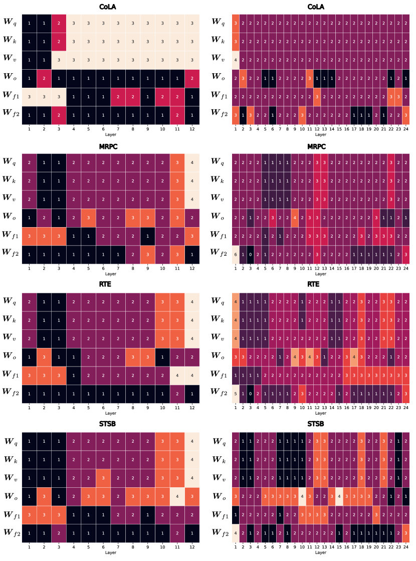
Figure 4: Rank distribution after initialization with EVA on four tasks of the GLUE benchmark (CoLA, MRPC, RTE, STSB) for $\text{DeBERTav3}_{\text{Base}}$ (left) and $\text{RoBERTa}_{\text{Large}}$ (right) with initial rank $r=2$.

Figure 5: Rank distribution after initialization with EVA on four tasks of the GLUE benchmark (CoLA, MRPC, RTE, STSB) for $\text{DeBERTav3}_{\text{Base}}$ (left) and $\text{RoBERTa}_{\text{Large}}$ (right) with initial rank $r=4$.

Figure 6: Rank distribution after initialization with EVA on four tasks of the GLUE benchmark (CoLA, MRPC, RTE, STSB) for $\text{DeBERTav3}_{\text{Base}}$ (left) and $\text{RoBERTa}_{\text{Large}}$ (right) with initial rank $r=8$.

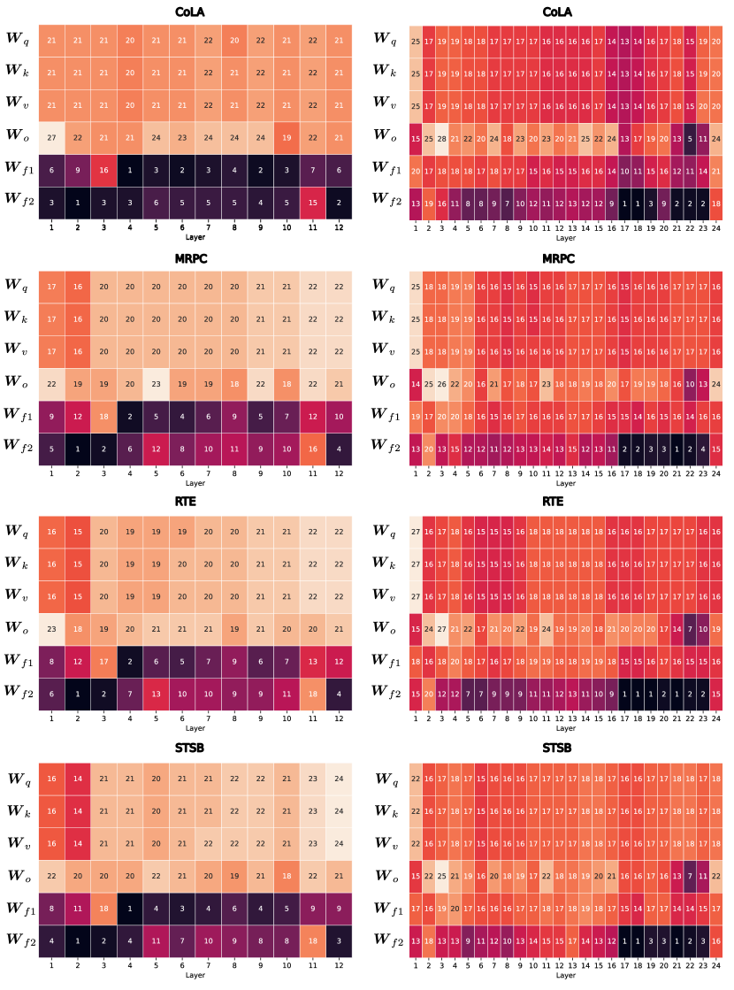
Figure 7: Rank distribution after initialization with EVA on four tasks of the GLUE benchmark (CoLA, MRPC, RTE, STSB) for $\text{DeBERTav3}_{\text{Base}}$ (left) and $\text{RoBERTa}_{\text{Large}}$ (right) with initial rank $r=16$.

Appendix D Image Classification

D.1 Dataset statistics

The VTAB-1K benchmark consists of 19 datasets, each containing a subset of 1000 examples of their respective samples. We summarize the dataset statistics for each dataset in Table 16. While the original train sizes of the datasets vary drastically, the 1K subset provides equal datasets across tasks. The number of classes also varies from as little as two to almost 400.

Table 16: Category, train size and classes of the VTAB-1K dataset.

Category	Dataset	Train size	Classes
Natural	Caltech101 (Fei-Fei et al., 2006)	3060	102
Natural	CIFAR-100 (Krizhevsky, 2009)	50000	100
Natural	DTD (Cimpoi et al., 2014)	3760	47
Natural	Flowers102 (Nilsback & Zisserman, 2008)	2040	102
Natural	Pets (Parkhi et al., 2012)	3680	37
Natural	Sun397 (Xiao et al., 2010)	87003	397
Natural	SVHN (Netzer et al., 2011)	73257	10
Specialized	EuroSAT (Helber et al., 2019)	21600	10
Specialized	Resisc45 (Cheng et al., 2017)	25200	45
Specialized	Patch Camelyon (Veeling et al., 2018)	294912	2
Specialized	Retinopathy (Kaggle & EyePacs, 2015)	46032	5
Structured	Clevr/count (Johnson et al., 2017)	70000	8
Structured	Clevr/distance (Johnson et al., 2017)	70000	6
Structured	dSprites/location (Matthey et al., 2017)	663552	16
Structured	dSprites/orientation (Matthey et al., 2017)	663552	16
Structured	SmallNORB/azimuth (LeCun et al., 2004)	36450	18
Structured	SmallNORB/elevation (LeCun et al., 2004)	36450	9
Structured	DMLab (Beattie et al., 2016)	88178	6
Structured	KITTI/distance (Geiger et al., 2013)	5711	4

D.2 Implementation details

We implemented a custom pipeline to fine-tune DINOv2-L/14 on VTAB-1K that supports LoRA, DoRA and EVA. To train AdaLora, PiSSA and OLoRA, we integrate their implementation from the peft library (Mangrulkar et al., 2022) into our pipeline. This pipeline is designed to be highly parallelizable and to be executed on individual GPUs. A single evaluation run of a L/14 model (all 19 datasets with hyperparameter tuning and evaluation) takes roughly 160 A100 GPU-hours but can be easily parallelized. A g/14 run takes roughly 140 H100 GPU-hours. A single evaluation run consists of 1140 hyperparameter tuning runs (19 datasets * 5 learning rates * 4 ranks * 3 seeds) and 95 evaluation runs (19 datasets * 5 seeds). Details to hyperparameter tuning are described below.

We use the original DINOv2 models (Oquab et al., 2023) and train a classification head on top of the [CLS] token, where we initialize the classification head weights with a normal distribution with $\sigma=\text{2e-5}$ and bias with zeros. We train the classification head, LoRA matrices and biases. Images are resized to $224\times 224$ resolution with bi-cubic interpolation and normalized with the per-channel mean and variance of ImageNet. We train all models in bfloat16 precision using the AdamW optimizer with a weight decay of $0.05$ for 30 epochs. We use a cosine learning rate schedule with a linear warm-up for the first 3 epochs. Batch size is set to 64 where we use gradient accumulation if the batchsize does not fit into GPU memory. Full fine-tuning uses a layer-wise lr decay (Clark et al., 2020) of 0.75.

D.3 Hyperparameter search

We first fine-tune on the 800 train samples of VTAB-1K datasets to find the best learning rate for the task. We sweep over $\texttt{learning\_rate}\in\{\text{2.5e-3},\text{1e-3},\text{7.5e-4},\text{5e-4},\text{2.5e-4}\}$ and $\texttt{rank}\in\{2,4,8,16\}$ and average the accuracy on the 200 validation samples over 3 different seeds to choose the best learning rate and rank for each dataset. For evaluation, we train on the union of train and validation set using 5 different seeds and report the average accuracy on the test set.

D.4 Additional results

To complement our main results in Table 5, we report the respective standard deviations in Table 17.

Table 17: Standard deviations for the VTAB-1K results (Table 5) over 5 seeds.

	Natural							Specialized				Structured
	Cifar100	Caltech101	DTD	Flower102	Pets	SVHN	Sun397	Camelyon	EuroSAT	Resisc45	Retinopathy	Clevr-Count	Clevr-Dist	DMLab	KITTI-Dist	dSpr-Loc	dSpr-Ori	sNORB-Azim	sNORB-Ele	Average
FFT	1.5	1.1	1.6	0.0	0.4	1.2	0.9	14.9	0.4	0.6	2.7	1.7	0.9	1.2	23.6	0.5	0.4	1.6	1.9	3.0
LoRA	0.2	0.4	0.2	0.0	0.3	36.4	0.1	0.5	0.3	0.1	0.4	0.2	0.3	0.5	1.2	0.4	0.4	0.7	0.4	2.3
AdaLoRA	0.0	0.2	0.4	0.0	0.1	0.4	0.1	0.3	0.3	0.2	0.3	0.3	0.2	0.3	0.8	0.8	0.3	0.3	0.4	0.3
PiSSA	0.2	0.4	0.3	0.0	0.2	0.5	0.2	0.7	0.2	0.1	0.4	0.3	0.4	0.2	0.7	0.3	0.5	0.4	0.5	0.3
OLoRA	0.3	0.3	0.4	0.0	0.3	29.4	0.1	0.3	0.1	0.2	0.2	0.5	0.1	0.3	24.6	0.3	0.4	0.3	0.8	3.1
EVA	0.2	0.5	0.2	0.0	0.1	0.3	0.1	0.3	0.2	0.3	0.4	0.5	0.3	0.6	0.6	0.5	0.5	0.2	0.5	0.3
DoRA	0.1	0.2	0.5	0.0	0.2	29.7	0.4	0.7	0.1	0.2	0.4	0.4	0.3	0.3	0.6	36.2	0.5	0.3	0.3	3.8
EVA+DoRA	0.2	1.3	0.6	0.0	0.3	0.5	0.3	0.4	0.2	0.3	0.3	0.4	0.4	12.8	1.3	2.5	0.3	0.6	0.6	1.2

Appendix E Decision Making

E.1 Dataset statistics

Meta-World (Yu et al., 2020) is an established benchmark in RL for multi-task continuous control. The benchmark consists of 50 challenging robotics tasks simulated using a Sawyer robotic arm in the MuJoCo physics engine (Todorov et al., 2012). All 50 tasks in Meta-World share the same underlying robotic arm. Therefore, all tasks share a common state (39-dimensional continuous vector) and action-space (6-dimensional). The reward functions in Meta-World are dense and based on the distance of the robotic arm to the goal location or objects. All episodes last for 200 environment interactions.

For our experiments on Meta-World, we leverage the datasets released by Schmied et al. (2023). We follow Wołczyk et al. (2021) and Schmied et al. (2023), and split the 50 tasks into 40 pre-training tasks (MT40) and 10 fine-tuning tasks (CW10). The CW10 tasks are:

hammer-v2, push-wall-v2, faucet-close-v2, push-back-v2, stick-pull-v2, stick-pull-v2, handle-press-side-v2, push-v2, shelf-place-v2, window-close-v2, and peg-unplug-side-v2.

The datasets contain 2M transitions for every of the 50 tasks, amounting to 80M transitions (320M tokens) across all training tasks. The average success rate and rewards across all MT40 tasks are 84% and 1414.62, respectively. We list the statistics per task in Table 18.

Table 18: Dataset statistics for all MT40 tasks from Schmied et al. (2023).

Task	$|\mathcal{S}|$	$|\mathcal{A}|$	Success Rate	Reward
assembly-v2	39	4	0.0	1206.9
basketball-v2	39	4	0.9	1375.95
bin-picking-v2	39	4	0.0	474.81
box-close-v2	39	4	0.0	759.15
button-press-topdown-v2	39	4	1.0	1299.24
button-press-topdown-wall-v2	39	4	1.0	1296.16
button-press-v2	39	4	1.0	1430.44
button-press-wall-v2	39	4	1.0	1508.16
coffee-button-v2	39	4	1.0	1499.17
coffee-pull-v2	39	4	1.0	1313.88
coffee-push-v2	39	4	0.6	508.14
dial-turn-v2	39	4	0.8	1674.29
disassemble-v2	39	4	1.0	1396.55
door-close-v2	39	4	1.0	1535.4
door-lock-v2	39	4	1.0	1712.65
door-open-v2	39	4	1.0	1544.32
door-unlock-v2	39	4	1.0	1733.64
drawer-close-v2	39	4	1.0	1845.92
drawer-open-v2	39	4	1.0	1710.65
faucet-open-v2	39	4	0.9	1727.98
hand-insert-v2	39	4	1.0	1607.17
handle-press-v2	39	4	1.0	1854.79
handle-pull-side-v2	39	4	1.0	1613.72
handle-pull-v2	39	4	1.0	1581.75
lever-pull-v2	39	4	1.0	1449.05
peg-insert-side-v2	39	4	1.0	1545.19
pick-out-of-hole-v2	39	4	1.0	1435.64
pick-place-v2	39	4	0.0	6.59
pick-place-wall-v2	39	4	0.1	702.59
plate-slide-back-side-v2	39	4	1.0	1766.24
plate-slide-back-v2	39	4	1.0	1773.56
plate-slide-side-v2	39	4	1.0	1663.35
plate-slide-v2	39	4	1.0	1667.35
reach-v2	39	4	1.0	1858.99
reach-wall-v2	39	4	1.0	1831.14
soccer-v2	39	4	0.4	445.84
stick-push-v2	39	4	1.0	1470.71
sweep-into-v2	39	4	1.0	1761.69
sweep-v2	39	4	1.0	1458.35
window-open-v2	39	4	1.0	1537.59
Average	-	-	0.84 ± 0.34	1414.62 ± 439.39

E.2 Implementation details

We implemented our pipeline that supports training for Meta-World on top of the code-base provided by Schmied et al. (2023). Our custom implementation supports training LoRA, DoRA and EVA. Furthermore, we leverage the peft library (Mangrulkar et al., 2022) to train the remaining methods.

For our experiments on Meta-World, we use a GPT2-like network architecture (Radford et al., 2019) with 4 Transformer layers, 8 heads, and hidden dimension of 512 resulting in 16M parameters. We use a context of 50 time steps, which amounts to a sequence length of 200, as each timestep contains states, actions, rewards and RTGs. We embed states, actions, rewards and return-to-gos (RTGs) using separate linear embedding layers per modality, as proposed by Chen et al. (2021a). We train with a batch size of 128 using a constant learning rate of $1e^{-4}$, 4000 linear warm-up steps followed by a cosine decay to $1e^{-6}$, using the AdamW optimizer (Loshchilov & Hutter, 2017). We employ gradient clipping of 0.25, weight decay of 0.01, and a dropout rate of 0.2. Our DT implementation employs global position embedding. For every task, we set the target return to the maximum return achieved in the respective training datasets, as proposed by (Schmied et al., 2023). Furthermore, we employ mixed-precision (Micikevicius et al., 2017) and flash-attention (Dao, 2023) to speed-up training.

We first pre-train a DT on all MT40 tasks (80M transitions) for 1M updates via next-action prediction by minimizing the mean-squared error. The resulting pre-trained model attains an average success rate of 80% across all MT40 tasks. Then we fine-tune the DT on each of the CW10 down-stream tasks for 100K updates with the same set of hyperparameters as used for pre-training. We run all our experiments on a public research cluster with 4xA100-40GB GPU nodes. A single fine-tuning run with EVA for one task takes roughly 1 hour on one A100.

E.3 Hyperparameter search

In line with previous experiments, we tune the rank for LoRA, DoRA, AdaLora and EVA, $\texttt{rank}\in\{2,4,8,16\}$. Further, we sweep over the same learning rates as for the GLUE tasks.

E.4 Additional results

In Table 19, we show the full comparison for all methods on CW10. EVA+DoRA consistently outperforms all competitors for the different rank budgets.

Table 19: Rank-wise comparison for all methods on CW10. We fine-tune a 12M DT on 10 tasks individually and report the mean success rates/rewards ($\pm$ standard error) for every task.

faucet-close

hammer

handle-press-side

peg-unplug-side

push-back

push

push-wall

shelf-place

stick-pull

window-close

Average

Method

Rank

FFT

-

$0.97_{\pm 0.03}$

$0.93_{\pm 0.03}$

$1.0_{\pm 0.0}$

$0.6_{\pm 0.05}$

$0.7_{\pm 0.12}$

$1.0_{\pm 0.0}$

$0.93_{\pm 0.03}$

$1.0_{\pm 0.0}$

$0.57_{\pm 0.07}$

$1.0_{\pm 0.0}$

$0.87_{\pm 0.03}$

LoRA

2

$1.0_{\pm 0.0}$

$1.0_{\pm 0.0}$

$1.0_{\pm 0.0}$

$0.6_{\pm 0.05}$

$0.57_{\pm 0.07}$

$0.97_{\pm 0.03}$

$0.93_{\pm 0.03}$

$1.0_{\pm 0.0}$

$0.37_{\pm 0.1}$

$1.{\pm 0.0}$

$0.84_{\pm 0.04}$

4

$1.0_{\pm 0.0}$

$0.97_{\pm 0.03}$

$1.0_{\pm 0.0}$

$0.47_{\pm 0.12}$

$0.63_{\pm 0.1}$

$0.97_{\pm 0.03}$

$1.0_{\pm 0.0}$

$1.0_{\pm 0.0}$

$0.23_{\pm 0.12}$

$1.0_{\pm 0.0}$

$0.83_{\pm 0.05}$

8

$1.0_{\pm 0.0}$

$0.97_{\pm 0.03}$

$1.0_{\pm 0.0}$

$0.43_{\pm 0.05}$

$0.4_{\pm 0.09}$

$0.97_{\pm 0.03}$

$0.93_{\pm 0.03}$

$1.0_{\pm 0.0}$

$0.23_{\pm 0.12}$

$1.0_{\pm 0.0}$

$0.79_{\pm 0.06}$

16

$1.0_{\pm 0.0}$

$0.97_{\pm 0.03}$

$1.0_{\pm 0.0}$

$0.43_{\pm 0.03}$

$0.47_{\pm 0.03}$

$1.0_{\pm 0.0}$

$0.97_{\pm 0.03}$

$1.0_{\pm 0.0}$

$0.4_{\pm 0.09}$

$1.0_{\pm 0.0}$

$0.82_{\pm 0.05}$

DoRA

2

$1.0_{\pm 0.0}$

$1.0_{\pm 0.0}$

$1.0_{\pm 0.0}$

$0.57_{\pm 0.05}$

$1.0_{\pm 0.0}$

$1.0_{\pm 0.0}$

$1.0_{\pm 0.0}$

$1.0_{\pm 0.0}$

$0.33_{\pm 0.11}$

$1.0_{\pm 0.0}$

$0.89_{\pm 0.04}$

4

$1.0_{\pm 0.0}$

$1.0_{\pm 0.0}$

$1.0_{\pm 0.0}$

$0.6_{\pm 0.12}$

$1.0_{\pm 0.0}$

$1.0_{\pm 0.0}$

$1.0_{\pm 0.0}$

$1.0_{\pm 0.0}$

$0.43_{\pm 0.12}$

$1.0_{\pm 0.0}$

$0.9_{\pm 0.04}$

8

$1.0_{\pm 0.0}$

$1.0_{\pm 0.0}$

$1.0_{\pm 0.0}$

$0.47_{\pm 0.12}$

$0.93_{\pm 0.05}$

$1.0_{\pm 0.0}$

$1.0_{\pm 0.0}$

$1.0_{\pm 0.0}$

$0.57_{\pm 0.15}$

$1.0_{\pm 0.0}$

$0.9_{\pm 0.04}$

16

$1.0_{\pm 0.0}$

$1.0_{\pm 0.0}$

$1.0_{\pm 0.0}$

$0.57_{\pm 0.12}$

$1.0_{\pm 0.0}$

$1.0_{\pm 0.0}$

$1.0_{\pm 0.0}$

$1.0_{\pm 0.0}$

$0.67_{\pm 0.15}$

$1.0_{\pm 0.0}$

$0.92_{\pm 0.03}$

AdaLoRA

2

$1.0_{\pm 0.0}$

$0.97_{\pm 0.03}$

$1.0_{\pm 0.0}$

$0.37_{\pm 0.05}$

$0.37_{\pm 0.05}$

$0.93_{\pm 0.05}$

$0.97_{\pm 0.03}$

$1.0_{\pm 0.0}$

$0.13_{\pm 0.07}$

$1.0_{\pm 0.0}$

$0.77_{\pm 0.06}$

4

$1.0_{\pm 0.0}$

$0.97_{\pm 0.03}$

$1.0_{\pm 0.0}$

$0.37_{\pm 0.07}$

$0.57_{\pm 0.1}$

$0.97_{\pm 0.03}$

$0.9_{\pm 0.08}$

$1.0_{\pm 0.0}$

$0.13_{\pm 0.07}$

$1.0_{\pm 0.0}$

$0.79_{\pm 0.06}$

8

$1.0_{\pm 0.0}$

$0.97_{\pm 0.03}$

$1.0_{\pm 0.0}$

$0.3_{\pm 0.05}$

$0.57_{\pm 0.14}$

$0.93_{\pm 0.03}$

$0.87_{\pm 0.07}$

$1.0_{\pm 0.0}$

$0.0_{\pm 0.0}$

$1.0_{\pm 0.0}$

$0.76_{\pm 0.06}$

16

$1.0_{\pm 0.0}$

$0.97_{\pm 0.03}$

$1.0_{\pm 0.0}$

$0.4_{\pm 0.09}$

$0.57_{\pm 0.12}$

$0.97_{\pm 0.03}$

$0.93_{\pm 0.05}$

$1.0_{\pm 0.0}$

$0.0_{\pm 0.0}$

$1.0_{\pm 0.0}$

$0.78_{\pm 0.06}$

oLoRA

2

$1.0_{\pm 0.0}$

$0.9_{\pm 0.05}$

$1.0_{\pm 0.0}$

$0.47_{\pm 0.03}$

$0.33_{\pm 0.03}$

$0.97_{\pm 0.03}$

$0.97_{0.03}$

$1.0_{\pm 0.0}$

$0.27_{\pm 0.11}$

$1.0_{\pm 0.0}$

$0.79_{\pm 0.05}$

4

$1.0_{\pm 0.0}$

$0.9_{\pm 0.05}$

$1.0_{\pm 0.0}$

$0.43_{\pm 0.03}$

$0.63_{\pm 0.12}$

$1.0_{\pm 0.0}$

$1.0_{0.0}$

$1.0_{\pm 0.0}$

$0.6_{\pm 0.12}$

$1.0_{\pm 0.0}$

$0.86_{\pm 0.04}$

8

$1.0_{\pm 0.0}$

$0.97_{\pm 0.03}$

$1.0_{\pm 0.0}$

$0.57_{\pm 0.1}$

$0.5_{\pm 0.08}$

$1.0_{\pm 0.0}$

$1.0_{0.0}$

$1.0_{\pm 0.0}$

$0.53_{\pm 0.14}$

$1.0_{\pm 0.0}$

$0.86_{\pm 0.04}$

16

$1.0_{\pm 0.0}$

$0.97_{\pm 0.03}$

$1.0_{\pm 0.0}$

$0.4_{\pm 0.05}$

$0.63_{\pm 0.03}$

$1.0_{\pm 0.0}$

$1.0_{0.0}$

$1.0_{\pm 0.0}$

$0.43_{\pm 0.05}$

$1.0_{\pm 0.0}$

$0.84_{\pm 0.04}$

PiSSa

2

$1.0_{\pm 0.0}$

$0.97_{\pm 0.03}$

$1.0_{\pm 0.0}$

$0.43_{\pm 0.11}$

$0.53_{\pm 0.07}$

$0.97_{\pm 0.03}$

$0.9_{0.08}$

$1.0_{\pm 0.0}$

$0.33_{\pm 0.17}$

$1.0_{\pm 0.0}$

$0.81_{\pm 0.05}$

4

$1.0_{\pm 0.0}$

$1.0_{\pm 0.0}$

$1.0_{\pm 0.0}$

$0.37_{\pm 0.07}$

$0.7_{\pm 0.05}$

$0.97_{\pm 0.03}$

$1.0_{0.0}$

$1.0_{\pm 0.0}$

$0.07_{\pm 0.05}$

$1.0_{\pm 0.0}$

$0.81_{\pm 0.06}$

8

$1.0_{\pm 0.0}$

$0.97_{\pm 0.03}$

$1.0_{\pm 0.0}$

$0.3_{\pm 0.0}$

$0.57_{\pm 0.03}$

$0.97_{\pm 0.03}$

$1.0_{0.0}$

$1.0_{\pm 0.0}$

$0.53_{\pm 0.1}$

$1.0_{\pm 0.0}$

$0.83_{\pm 0.05}$

16

$1.0_{\pm 0.0}$

$0.93_{\pm 0.03}$

$1.0_{\pm 0.0}$

$0.33_{\pm 0.12}$

$0.47_{\pm 0.03}$

$1.0_{\pm 0.0}$

$0.97_{0.03}$

$1.0_{\pm 0.0}$

$0.47_{\pm 0.11}$

$1.0_{\pm 0.0}$

$0.82_{\pm 0.05}$

EVA

2

$1.0_{\pm 0.0}$

$0.97_{\pm 0.03}$

$1.0_{\pm 0.0}$

$0.43_{\pm 0.07}$

$0.77_{\pm 0.05}$

$0.97_{\pm 0.03}$

$1.0_{\pm 0.0}$

$1.0_{\pm 0.0}$

$0.63_{\pm 0.07}$

$1.0_{\pm 0.0}$

$0.88_{\pm 0.04}$

4

$1.0_{\pm 0.0}$

$0.97_{\pm 0.03}$

$1.0_{\pm 0.0}$

$0.43_{\pm 0.05}$

$0.47_{\pm 0.12}$

$1.0_{\pm 0.0}$

$0.97_{\pm 0.03}$

$1.0_{\pm 0.0}$

$0.23_{\pm 0.05}$

$1.0_{\pm 0.0}$

$0.81_{\pm 0.05}$

8

$1.0_{\pm 0.0}$

$0.97_{\pm 0.03}$

$1.0_{\pm 0.0}$

$0.63_{\pm 0.03}$

$0.7_{\pm 0.08}$

$1.0_{\pm 0.0}$

$1.0_{\pm 0.0}$

$1.0_{\pm 0.0}$

$0.23_{\pm 0.03}$

$1.0_{\pm 0.0}$

$0.85_{\pm 0.05}$

16

$1.0_{\pm 0.0}$

$0.97_{\pm 0.03}$

$1.0_{\pm 0.0}$

$0.53_{\pm 0.03}$

$0.77_{\pm 0.07}$

$1.0_{\pm 0.0}$

$1.0_{\pm 0.0}$

$1.0_{\pm 0.0}$

$0.0_{\pm 0.0}$

$1.0_{\pm 0.0}$

$0.83_{\pm 0.06}$

EVA + DoRA

2

$1.0_{\pm 0.0}$

$1.0_{\pm 0.0}$

$1.0_{\pm 0.0}$

$0.8_{\pm 0.08}$

$0.97_{\pm 0.03}$

$1.0_{\pm 0.0}$

$1.0_{\pm 0.0}$

$1.0_{\pm 0.0}$

$0.43_{\pm 0.12}$

$1.0_{\pm 0.0}$

$0.92_{\pm 0.03}$

4

$1.0_{\pm 0.0}$

$1.0_{\pm 0.0}$

$1.0_{\pm 0.0}$

$0.8_{\pm 0.05}$

$0.93_{\pm 0.03}$

$1.0_{\pm 0.0}$

$1.0_{\pm 0.0}$

$1.0_{\pm 0.0}$

$0.63_{\pm 0.03}$

$1.0_{\pm 0.0}$

$0.94_{\pm 0.02}$

8

$1.0_{\pm 0.0}$

$1.0_{\pm 0.0}$

$1.0_{\pm 0.0}$

$0.63_{\pm 0.19}$

$0.87_{\pm 0.07}$

$1.0_{\pm 0.0}$

$1.0_{\pm 0.0}$

$1.0_{\pm 0.0}$

$0.57_{\pm 0.03}$

$1.0_{\pm 0.0}$

$0.91_{\pm 0.04}$

16

$1.0_{\pm 0.0}$

$1.0_{\pm 0.0}$

$1.0_{\pm 0.0}$

$0.67_{\pm 0.2}$

$1.0_{\pm 0.0}$

$1.0_{\pm 0.0}$

$1.0_{\pm 0.0}$

$1.0_{\pm 0.0}$

$0.5_{\pm 0.16}$

$1.0_{\pm 0.0}$

$0.92_{\pm 0.04}$

Appendix F SVD convergence analysis

F.1 Batch Size invariance

We conduct an analysis on the convergence of the components obtained via SVD. Specifically, we investigate the difference in components according to cosine similarity across different batch sizes. Previously we have seen that the components obtained across different batch orderings are heavily correlated. In Figure 8 we visualize the cosine similarities between the SVD components for different batch sizes, namely 4, 8, 16, and 32 for Llama-2-7B on the MetaMathQA dataset. We observe that the components correlate strongly and remain mostly invariant to the batch size. This indicates that smaller batch sizes may be used for obtaining the initialization which results in less computational overhead. In the case of Llama-2-7B on MetaMathQA, this means that we can use a batch size of 4 since it induces a computational overhead of around 100 seconds. Afterwards we can continue the fine-tuning process with a larger batch size.

F.2 Excluding ignored tokens for SVD

For some datasets we notice that masking out tokens for the SVD computation which are ignored for the loss calculation during finetuning can be advantageous. This can however result in a significant reduction of the effective batch size for SVD if the number of completion tokens is small. An example where this is the case in our experiments are the common sense reasoning tasks which have long prompts but completion tokens are only one word per sample. This setting can lead to cases were SVD does not converge for lower batch sizes. We therefore do not mask out the prompt tokens for the common sense reasoning tasks, but apply masking for the math and coding tasks. For the multi-turn coding tasks (Table 10), we found masking to significantly improve the performance. In this setup we mask out all tokens except for the assistant tokens.

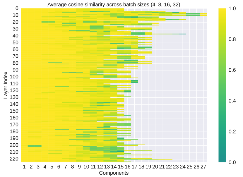
Figure 8: Average cosine similarity between components obtained via SVD on minibatches of activation vectors across different batch sizes. The components strongly correlate indicating that the SVD computation is mostly invariant to the batch size and returns mostly the same components.

Appendix G Rank re-distribution analysis

To illuminate the rank re-distribution process, we visualize the resulting ranks for each weight matrix after SVD for Llama-2-7B on the MetaMathQA dataset for different values of $\rho$. Setting $\rho=1$ results in a uniform rank distribution as in standard LoRA. However, setting $\rho>1$ alters the number of ranks per weight matrix. In Figure 9 we visualize the number of ranks assigned to each weight matrix for different values of $\rho>1$ and in Figure 10 we visualize the corresponding deltas. Both visualizations clearly illustrate that the most change occurs for values of $\rho<1.5$. Setting $\rho$ to higher values results in less and less change. Interestingly, some ranks still change when going from $\rho=2.5$ to $\rho=3$. Finally, we conduct hyperparameter search in which we search over different values of $\rho\in\{1,1.1,1.2,1.3,1.4,1.5,1.6,1.7,1.8,1.9,2,2.5,3\}$. We report the results in Figure 11. We find that for Llama-2-7B on MetaMathQA a uniform distribution performs favorably. The second-best performance is shared by $\rho=1.5$ and $\rho=2$. Therefore, we always search for $\rho=1$ and $\rho=2$ for all our remaining experiments when we apply EVA and select the best performing one.

Figure 9: The resulting rank allocation per weight matrix in each layer for Llama-2-7B on the MetaMathQA dataset with different values of $\rho$. The first row represents a uniform distribution where each weight matrix receives the same rank $r=16$. The most change occurs for $\rho<1.5$. The re-distribution converges for larger values of $\rho$.

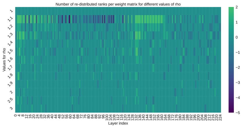
Figure 10: Deltas between rank distributions per weight matrix in each layer for Llama-2-7B on the MetaMathQA dataset with different values of $\rho$. The first row represents a uniform distribution where each weight matrix receives the same rank $r=16$. The most change occurs in the range $\rho\in[1,1.5]$. Larger values of $\rho$ do not induce additional significant changes to the rank distribution.

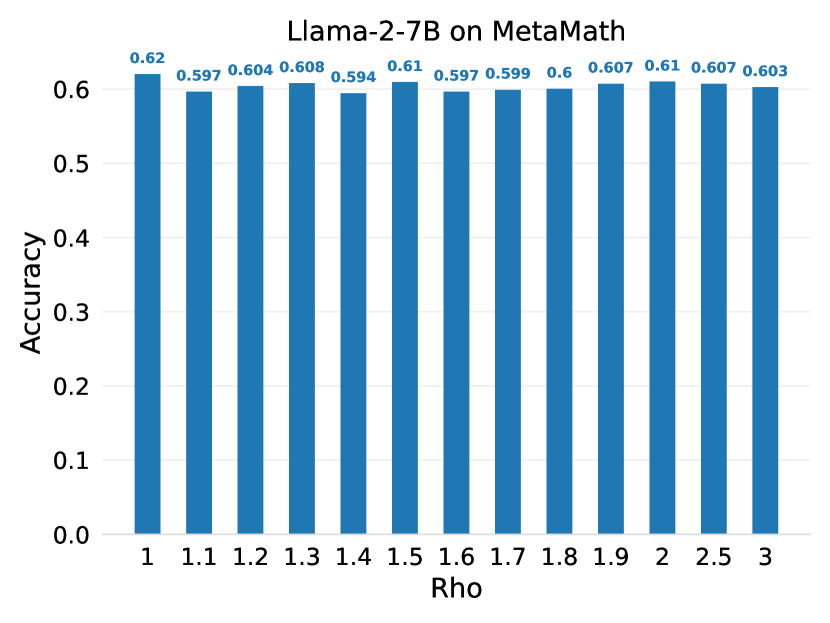
Figure 11: Accuracy for different values of $\rho$ when fine-tuning Llama-2-7B on the MetaMathQA dataset.

References

- Aghajanyan et al. (2021) Aghajanyan, A., Gupta, S., and Zettlemoyer, L. Intrinsic dimensionality explains the effectiveness of language model fine-tuning. In Zong, C., Xia, F., Li, W., and Navigli, R. (eds.), Proceedings of the 59th Annual Meeting of the Association for Computational Linguistics and the 11th International Joint Conference on Natural Language Processing, ACL/IJCNLP 2021, (Volume 1: Long Papers), Virtual Event, August 1-6, 2021, pp. 7319–7328. Association for Computational Linguistics, 2021. doi: 10.18653/v1/2021.acl-long.568.
- Austin et al. (2021) Austin, J., Odena, A., Nye, M., Bosma, M., Michalewski, H., Dohan, D., Jiang, E., Cai, C., Terry, M., Le, Q., et al. Program synthesis with large language models. arXiv preprint arXiv:2108.07732, 2021.
- Babakniya et al. (2023) Babakniya, S., Elkordy, A. R., Ezzeldin, Y. H., Liu, Q., Song, K., El-Khamy, M., and Avestimehr, S. Slora: Federated parameter efficient fine-tuning of language models. CoRR, abs/2308.06522, 2023. doi: 10.48550/ARXIV.2308.06522.
- Beattie et al. (2016) Beattie, C., Leibo, J. Z., Teplyashin, D., Ward, T., Wainwright, M., Küttler, H., Lefrancq, A., Green, S., Valdés, V., Sadik, A., Schrittwieser, J., Anderson, K., York, S., Cant, M., Cain, A., Bolton, A., Gaffney, S., King, H., Hassabis, D., Legg, S., and Petersen, S. Deepmind lab. CoRR, abs/1612.03801, 2016.
- Bisk et al. (2020) Bisk, Y., Zellers, R., Bras, R. L., Gao, J., and Choi, Y. Piqa: Reasoning about physical commonsense in natural language. In Thirty-Fourth AAAI Conference on Artificial Intelligence, 2020.
- Bommasani et al. (2021) Bommasani, R., Hudson, D. A., Adeli, E., Altman, R. B., Arora, S., von Arx, S., Bernstein, M. S., Bohg, J., Bosselut, A., Brunskill, E., Brynjolfsson, E., Buch, S., Card, D., Castellon, R., Chatterji, N. S., Chen, A. S., Creel, K., Davis, J. Q., Demszky, D., Donahue, C., Doumbouya, M., Durmus, E., Ermon, S., Etchemendy, J., Ethayarajh, K., Fei-Fei, L., Finn, C., Gale, T., Gillespie, L., Goel, K., Goodman, N. D., Grossman, S., Guha, N., Hashimoto, T., Henderson, P., Hewitt, J., Ho, D. E., Hong, J., Hsu, K., Huang, J., Icard, T., Jain, S., Jurafsky, D., Kalluri, P., Karamcheti, S., Keeling, G., Khani, F., Khattab, O., Koh, P. W., Krass, M. S., Krishna, R., Kuditipudi, R., and et al. On the opportunities and risks of foundation models. CoRR, abs/2108.07258, 2021.
- Brohan et al. (2023) Brohan, A., Brown, N., Carbajal, J., Chebotar, Y., Dabis, J., Finn, C., Gopalakrishnan, K., Hausman, K., Herzog, A., Hsu, J., Ibarz, J., Ichter, B., Irpan, A., Jackson, T., Jesmonth, S., Joshi, N. J., Julian, R., Kalashnikov, D., Kuang, Y., Leal, I., Lee, K., Levine, S., Lu, Y., Malla, U., Manjunath, D., Mordatch, I., Nachum, O., Parada, C., Peralta, J., Perez, E., Pertsch, K., Quiambao, J., Rao, K., Ryoo, M. S., Salazar, G., Sanketi, P. R., Sayed, K., Singh, J., Sontakke, S., Stone, A., Tan, C., Tran, H. T., Vanhoucke, V., Vega, S., Vuong, Q., Xia, F., Xiao, T., Xu, P., Xu, S., Yu, T., and Zitkovich, B. RT-1: robotics transformer for real-world control at scale. In Bekris, K. E., Hauser, K., Herbert, S. L., and Yu, J. (eds.), Robotics: Science and Systems XIX, Daegu, Republic of Korea, July 10-14, 2023, 2023. doi: 10.15607/RSS.2023.XIX.025.
- Büyükakyüz (2024) Büyükakyüz, K. Olora: Orthonormal low-rank adaptation of large language models. CoRR, abs/2406.01775, 2024. doi: 10.48550/ARXIV.2406.01775.
- Chavan et al. (2023) Chavan, A., Liu, Z., Gupta, D. K., Xing, E. P., and Shen, Z. One-for-all: Generalized lora for parameter-efficient fine-tuning. CoRR, abs/2306.07967, 2023. doi: 10.48550/ARXIV.2306.07967.
- Chen et al. (2021a) Chen, L., Lu, K., Rajeswaran, A., Lee, K., Grover, A., Laskin, M., Abbeel, P., Srinivas, A., and Mordatch, I. Decision transformer: Reinforcement learning via sequence modeling. Advances in neural information processing systems, 34:15084–15097, 2021a.
- Chen et al. (2021b) Chen, M., Tworek, J., Jun, H., Yuan, Q., de Oliveira Pinto, H. P., Kaplan, J., Edwards, H., Burda, Y., Joseph, N., Brockman, G., Ray, A., Puri, R., Krueger, G., Petrov, M., Khlaaf, H., Sastry, G., Mishkin, P., Chan, B., Gray, S., Ryder, N., Pavlov, M., Power, A., Kaiser, L., Bavarian, M., Winter, C., Tillet, P., Such, F. P., Cummings, D., Plappert, M., Chantzis, F., Barnes, E., Herbert-Voss, A., Guss, W. H., Nichol, A., Paino, A., Tezak, N., Tang, J., Babuschkin, I., Balaji, S., Jain, S., Saunders, W., Hesse, C., Carr, A. N., Leike, J., Achiam, J., Misra, V., Morikawa, E., Radford, A., Knight, M., Brundage, M., Murati, M., Mayer, K., Welinder, P., McGrew, B., Amodei, D., McCandlish, S., Sutskever, I., and Zaremba, W. Evaluating large language models trained on code, 2021b.
- Cheng et al. (2017) Cheng, G., Han, J., and Lu, X. Remote sensing image scene classification: Benchmark and state of the art. Proc. IEEE, 105(10):1865–1883, 2017. doi: 10.1109/JPROC.2017.2675998.
- Christopher et al. (2019) Christopher, C., Kenton, L., Ming-Wei, C., Tom, K., Michael, C., and Kristina, T. Boolq: Exploring the surprising difficulty of natural yes/no questions. In NAACL, 2019.
- Cimpoi et al. (2014) Cimpoi, M., Maji, S., Kokkinos, I., Mohamed, S., and Vedaldi, A. Describing textures in the wild. In 2014 IEEE Conference on Computer Vision and Pattern Recognition, CVPR 2014, Columbus, OH, USA, June 23-28, 2014, pp. 3606–3613. IEEE Computer Society, 2014. doi: 10.1109/CVPR.2014.461.
- Clark et al. (2020) Clark, K., Luong, M., Le, Q. V., and Manning, C. D. ELECTRA: pre-training text encoders as discriminators rather than generators. In 8th International Conference on Learning Representations, ICLR 2020, Addis Ababa, Ethiopia, April 26-30, 2020. OpenReview.net, 2020.
- Clark et al. (2018) Clark, P., Cowhey, I., Etzioni, O., Khot, T., Sabharwal, A., Schoenick, C., and Tafjord, O. Think you have solved question answering? try arc, the ai2 reasoning challenge. arXiv:1803.05457v1, 2018.
- Cobbe et al. (2021) Cobbe, K., Kosaraju, V., Bavarian, M., Chen, M., Jun, H., Kaiser, L., Plappert, M., Tworek, J., Hilton, J., Nakano, R., Hesse, C., and Schulman, J. Training verifiers to solve math word problems, 2021.
- Dao (2023) Dao, T. Flashattention-2: Faster attention with better parallelism and work partitioning. arXiv preprint arXiv:2307.08691, 2023.
- Dehghani et al. (2023) Dehghani, M., Djolonga, J., Mustafa, B., Padlewski, P., Heek, J., Gilmer, J., Steiner, A. P., Caron, M., Geirhos, R., Alabdulmohsin, I., Jenatton, R., Beyer, L., Tschannen, M., Arnab, A., Wang, X., Ruiz, C. R., Minderer, M., Puigcerver, J., Evci, U., Kumar, M., van Steenkiste, S., Elsayed, G. F., Mahendran, A., Yu, F., Oliver, A., Huot, F., Bastings, J., Collier, M., Gritsenko, A. A., Birodkar, V., Vasconcelos, C. N., Tay, Y., Mensink, T., Kolesnikov, A., Pavetic, F., Tran, D., Kipf, T., Lucic, M., Zhai, X., Keysers, D., Harmsen, J. J., and Houlsby, N. Scaling vision transformers to 22 billion parameters. In Krause, A., Brunskill, E., Cho, K., Engelhardt, B., Sabato, S., and Scarlett, J. (eds.), International Conference on Machine Learning, ICML 2023, 23-29 July 2023, Honolulu, Hawaii, USA, volume 202 of Proceedings of Machine Learning Research, pp. 7480–7512. PMLR, 2023.
- Dettmers et al. (2022) Dettmers, T., Lewis, M., Belkada, Y., and Zettlemoyer, L. Gpt3.int8(): 8-bit matrix multiplication for transformers at scale. In Koyejo, S., Mohamed, S., Agarwal, A., Belgrave, D., Cho, K., and Oh, A. (eds.), Advances in Neural Information Processing Systems, volume 35, pp. 30318–30332. Curran Associates, Inc., 2022.
- Dettmers et al. (2023) Dettmers, T., Pagnoni, A., Holtzman, A., and Zettlemoyer, L. Qlora: Efficient finetuning of quantized llms. In Oh, A., Naumann, T., Globerson, A., Saenko, K., Hardt, M., and Levine, S. (eds.), Advances in Neural Information Processing Systems 36: Annual Conference on Neural Information Processing Systems 2023, NeurIPS 2023, New Orleans, LA, USA, December 10 - 16, 2023, 2023.
- Dosovitskiy et al. (2021) Dosovitskiy, A., Beyer, L., Kolesnikov, A., Weissenborn, D., Zhai, X., Unterthiner, T., Dehghani, M., Minderer, M., Heigold, G., Gelly, S., Uszkoreit, J., and Houlsby, N. An image is worth 16x16 words: Transformers for image recognition at scale. In 9th International Conference on Learning Representations, ICLR 2021, Virtual Event, Austria, May 3-7, 2021. OpenReview.net, 2021.
- Dubey et al. (2024) Dubey, A., Jauhri, A., Pandey, A., Kadian, A., Al-Dahle, A., Letman, A., Mathur, A., Schelten, A., Yang, A., Fan, A., Goyal, A., Hartshorn, A., Yang, A., Mitra, A., Sravankumar, A., Korenev, A., Hinsvark, A., Rao, A., Zhang, A., Rodriguez, A., Gregerson, A., Spataru, A., Rozière, B., Biron, B., Tang, B., Chern, B., Caucheteux, C., Nayak, C., Bi, C., Marra, C., McConnell, C., Keller, C., Touret, C., Wu, C., Wong, C., Ferrer, C. C., Nikolaidis, C., Allonsius, D., Song, D., Pintz, D., Livshits, D., Esiobu, D., Choudhary, D., Mahajan, D., Garcia-Olano, D., Perino, D., Hupkes, D., Lakomkin, E., AlBadawy, E., Lobanova, E., Dinan, E., Smith, E. M., Radenovic, F., Zhang, F., Synnaeve, G., Lee, G., Anderson, G. L., Nail, G., Mialon, G., Pang, G., Cucurell, G., Nguyen, H., Korevaar, H., Xu, H., Touvron, H., Zarov, I., Ibarra, I. A., Kloumann, I. M., Misra, I., Evtimov, I., Copet, J., Lee, J., Geffert, J., Vranes, J., Park, J., Mahadeokar, J., Shah, J., van der Linde, J., Billock, J., Hong, J., Lee, J., Fu, J., Chi, J., Huang, J., Liu, J., Wang, J., Yu, J., Bitton, J., Spisak, J., Park, J., Rocca, J., Johnstun, J., Saxe, J., Jia, J., Alwala, K. V., Upasani, K., Plawiak, K., Li, K., Heafield, K., Stone, K., and et al. The llama 3 herd of models. CoRR, abs/2407.21783, 2024. doi: 10.48550/ARXIV.2407.21783.
- Fei-Fei et al. (2006) Fei-Fei, L., Fergus, R., and Perona, P. One-shot learning of object categories. IEEE Trans. Pattern Anal. Mach. Intell., 28(4):594–611, 2006. doi: 10.1109/TPAMI.2006.79.
- Fisher (1936) Fisher, R. A. The use of multiple measurements in taxonomic problems. Annals Eugenics, 7:179–188, 1936.
- Gao et al. (2024) Gao, L., Tow, J., Abbasi, B., Biderman, S., Black, S., DiPofi, A., Foster, C., Golding, L., Hsu, J., Le Noac’h, A., Li, H., McDonell, K., Muennighoff, N., Ociepa, C., Phang, J., Reynolds, L., Schoelkopf, H., Skowron, A., Sutawika, L., Tang, E., Thite, A., Wang, B., Wang, K., and Zou, A. A framework for few-shot language model evaluation, 07 2024.
- Gauch et al. (2022) Gauch, M., Beck, M., Adler, T., Kotsur, D., Fiel, S., Eghbal-zadeh, H., Brandstetter, J., Kofler, J., Holzleitner, M., Zellinger, W., Klotz, D., Hochreiter, S., and Lehner, S. Few-shot learning by dimensionality reduction in gradient space. In Chandar, S., Pascanu, R., and Precup, D. (eds.), Conference on Lifelong Learning Agents, CoLLAs 2022, 22-24 August 2022, McGill University, Montréal, Québec, Canada, volume 199 of Proceedings of Machine Learning Research, pp. 1043–1064. PMLR, 2022.
- Geiger et al. (2013) Geiger, A., Lenz, P., Stiller, C., and Urtasun, R. Vision meets robotics: The KITTI dataset. Int. J. Robotics Res., 32(11):1231–1237, 2013. doi: 10.1177/0278364913491297.
- Glorot & Bengio (2010) Glorot, X. and Bengio, Y. Understanding the difficulty of training deep feedforward neural networks. In Teh, Y. W. and Titterington, D. M. (eds.), Proceedings of the Thirteenth International Conference on Artificial Intelligence and Statistics, AISTATS 2010, Chia Laguna Resort, Sardinia, Italy, May 13-15, 2010, volume 9 of JMLR Proceedings, pp. 249–256. JMLR.org, 2010.
- Gur-Ari et al. (2018) Gur-Ari, G., Roberts, D. A., and Dyer, E. Gradient descent happens in a tiny subspace. CoRR, abs/1812.04754, 2018.
- Halko et al. (2011) Halko, N., Martinsson, P., and Tropp, J. A. Finding structure with randomness: Probabilistic algorithms for constructing approximate matrix decompositions. SIAM Rev., 53(2):217–288, 2011. doi: 10.1137/090771806.
- Hayou et al. (2024a) Hayou, S., Ghosh, N., and Yu, B. The impact of initialization on lora finetuning dynamics, 2024a.
- Hayou et al. (2024b) Hayou, S., Ghosh, N., and Yu, B. Lora+: Efficient low rank adaptation of large models, 2024b.
- He et al. (2015) He, K., Zhang, X., Ren, S., and Sun, J. Delving deep into rectifiers: Surpassing human-level performance on imagenet classification. In 2015 IEEE International Conference on Computer Vision, ICCV 2015, Santiago, Chile, December 7-13, 2015, pp. 1026–1034. IEEE Computer Society, 2015. doi: 10.1109/ICCV.2015.123.
- He et al. (2023) He, P., Gao, J., and Chen, W. Debertav3: Improving deberta using electra-style pre-training with gradient-disentangled embedding sharing. In The Eleventh International Conference on Learning Representations, ICLR 2023, Kigali, Rwanda, May 1-5, 2023. OpenReview.net, 2023.
- Helber et al. (2019) Helber, P., Bischke, B., Dengel, A., and Borth, D. Eurosat: A novel dataset and deep learning benchmark for land use and land cover classification. IEEE J. Sel. Top. Appl. Earth Obs. Remote. Sens., 12(7):2217–2226, 2019. doi: 10.1109/JSTARS.2019.2918242.
- Hu et al. (2022) Hu, E. J., Shen, Y., Wallis, P., Allen-Zhu, Z., Li, Y., Wang, S., Wang, L., and Chen, W. Lora: Low-rank adaptation of large language models. In The Tenth International Conference on Learning Representations, ICLR 2022, Virtual Event, April 25-29, 2022. OpenReview.net, 2022.
- Hu et al. (2023) Hu, Z., Wang, L., Lan, Y., Xu, W., Lim, E.-P., Bing, L., Xu, X., Poria, S., and Lee, R. LLM-adapters: An adapter family for parameter-efficient fine-tuning of large language models. In Proceedings of the 2023 Conference on Empirical Methods in Natural Language Processing, pp. 5254–5276, Singapore, December 2023. Association for Computational Linguistics. doi: 10.18653/v1/2023.emnlp-main.319.
- Johnson et al. (2017) Johnson, J., Hariharan, B., van der Maaten, L., Fei-Fei, L., Zitnick, C. L., and Girshick, R. B. CLEVR: A diagnostic dataset for compositional language and elementary visual reasoning. In 2017 IEEE Conference on Computer Vision and Pattern Recognition, CVPR 2017, Honolulu, HI, USA, July 21-26, 2017, pp. 1988–1997. IEEE Computer Society, 2017. doi: 10.1109/CVPR.2017.215.
- Kaggle & EyePacs (2015) Kaggle and EyePacs. Kaggle diabetic retinopathy detection, July 2015.
- Kalajdzievski (2023) Kalajdzievski, D. A rank stabilization scaling factor for fine-tuning with lora. CoRR, abs/2312.03732, 2023. doi: 10.48550/ARXIV.2312.03732.
- Kopiczko et al. (2024) Kopiczko, D. J., Blankevoort, T., and Asano, Y. M. ELoRA: Efficient low-rank adaptation with random matrices. In The Twelfth International Conference on Learning Representations, 2024.
- Krähenbühl et al. (2016) Krähenbühl, P., Doersch, C., Donahue, J., and Darrell, T. Data-dependent initializations of convolutional neural networks. In Bengio, Y. and LeCun, Y. (eds.), 4th International Conference on Learning Representations, ICLR 2016, San Juan, Puerto Rico, May 2-4, 2016, Conference Track Proceedings, 2016.
- Krizhevsky (2009) Krizhevsky, A. Learning multiple layers of features from tiny images. CoRR, pp. 32–33, 2009.
- LeCun et al. (2004) LeCun, Y., Huang, F. J., and Bottou, L. Learning methods for generic object recognition with invariance to pose and lighting. In 2004 IEEE Computer Society Conference on Computer Vision and Pattern Recognition (CVPR 2004), with CD-ROM, 27 June - 2 July 2004, Washington, DC, USA, pp. 97–104. IEEE Computer Society, 2004. doi: 10.1109/CVPR.2004.144.
- Li et al. (2023) Li, Y., Yu, Y., Liang, C., He, P., Karampatziakis, N., Chen, W., and Zhao, T. Loftq: Lora-fine-tuning-aware quantization for large language models. CoRR, abs/2310.08659, 2023. doi: 10.48550/ARXIV.2310.08659.
- Liu et al. (2022) Liu, H., Tam, D., Muqeeth, M., Mohta, J., Huang, T., Bansal, M., and Raffel, C. Few-shot parameter-efficient fine-tuning is better and cheaper than in-context learning. In Koyejo, S., Mohamed, S., Agarwal, A., Belgrave, D., Cho, K., and Oh, A. (eds.), Advances in Neural Information Processing Systems 35: Annual Conference on Neural Information Processing Systems 2022, NeurIPS 2022, New Orleans, LA, USA, November 28 - December 9, 2022, 2022.
- Liu et al. (2023) Liu, J., Xia, C. S., Wang, Y., and Zhang, L. Is your code generated by chatGPT really correct? rigorous evaluation of large language models for code generation. In Thirty-seventh Conference on Neural Information Processing Systems, 2023.
- Liu et al. (2024a) Liu, S., Wang, C., Yin, H., Molchanov, P., Wang, Y. F., Cheng, K., and Chen, M. Dora: Weight-decomposed low-rank adaptation. CoRR, abs/2402.09353, 2024a. doi: 10.48550/ARXIV.2402.09353.
- Liu et al. (2019) Liu, Y., Ott, M., Goyal, N., Du, J., Joshi, M., Chen, D., Levy, O., Lewis, M., Zettlemoyer, L., and Stoyanov, V. Roberta: A robustly optimized BERT pretraining approach. CoRR, abs/1907.11692, 2019.
- Liu et al. (2024b) Liu, Z., Lyn, J., Zhu, W., Tian, X., and Graham, Y. Alora: Allocating low-rank adaptation for fine-tuning large language models. In Duh, K., Gómez-Adorno, H., and Bethard, S. (eds.), Proceedings of the 2024 Conference of the North American Chapter of the Association for Computational Linguistics: Human Language Technologies (Volume 1: Long Papers), NAACL 2024, Mexico City, Mexico, June 16-21, 2024, pp. 622–641. Association for Computational Linguistics, 2024b. doi: 10.18653/V1/2024.NAACL-LONG.35.
- Loshchilov & Hutter (2017) Loshchilov, I. and Hutter, F. Fixing weight decay regularization in adam. CoRR, abs/1711.05101, 2017.
- Mangrulkar et al. (2022) Mangrulkar, S., Gugger, S., Debut, L., Belkada, Y., Paul, S., and Bossan, B. Peft: State-of-the-art parameter-efficient fine-tuning methods, 2022.
- Matthey et al. (2017) Matthey, L., Higgins, I., Hassabis, D., and Lerchner, A. dsprites: Disentanglement testing sprites dataset. https://github.com/deepmind/dsprites-dataset/, 2017.
- Meng et al. (2024) Meng, F., Wang, Z., and Zhang, M. Pissa: Principal singular values and singular vectors adaptation of large language models, 2024.
- Meo et al. (2024) Meo, C., Sycheva, K., Goyal, A., and Dauwels, J. Bayesian-lora: Lora based parameter efficient fine-tuning using optimal quantization levels and rank values trough differentiable bayesian gates. CoRR, abs/2406.13046, 2024. doi: 10.48550/ARXIV.2406.13046.
- Micikevicius et al. (2017) Micikevicius, P., Narang, S., Alben, J., Diamos, G., Elsen, E., Garcia, D., Ginsburg, B., Houston, M., Kuchaiev, O., Venkatesh, G., et al. Mixed precision training. arXiv preprint arXiv:1710.03740, 2017.
- Mihaylov et al. (2018) Mihaylov, T., Clark, P., Khot, T., and Sabharwal, A. Can a suit of armor conduct electricity? a new dataset for open book question answering. In EMNLP, 2018.
- Mishkin & Matas (2016) Mishkin, D. and Matas, J. All you need is a good init. In Bengio, Y. and LeCun, Y. (eds.), 4th International Conference on Learning Representations, ICLR 2016, San Juan, Puerto Rico, May 2-4, 2016, Conference Track Proceedings, 2016.
- Netzer et al. (2011) Netzer, Y., Wang, T., Coates, A., Bissacco, A., Wu, B., and Ng, A. Y. Reading digits in natural images with unsupervised feature learning. In NIPS Workshop on Deep Learning and Unsupervised Feature Learning 2011, 2011.
- Nikdan et al. (2024) Nikdan, M., Tabesh, S., and Alistarh, D. Rosa: Accurate parameter-efficient fine-tuning via robust adaptation. CoRR, abs/2401.04679, 2024. doi: 10.48550/ARXIV.2401.04679.
- Nilsback & Zisserman (2008) Nilsback, M. and Zisserman, A. Automated flower classification over a large number of classes. In Sixth Indian Conference on Computer Vision, Graphics & Image Processing, ICVGIP 2008, Bhubaneswar, India, 16-19 December 2008, pp. 722–729. IEEE Computer Society, 2008. doi: 10.1109/ICVGIP.2008.47.
- OpenAI (2023) OpenAI. GPT-4 technical report. CoRR, abs/2303.08774, 2023. doi: 10.48550/ARXIV.2303.08774.
- Oquab et al. (2023) Oquab, M., Darcet, T., Moutakanni, T., Vo, H., Szafraniec, M., Khalidov, V., Fernandez, P., Haziza, D., Massa, F., El-Nouby, A., Assran, M., Ballas, N., Galuba, W., Howes, R., Huang, P., Li, S., Misra, I., Rabbat, M. G., Sharma, V., Synnaeve, G., Xu, H., Jégou, H., Mairal, J., Labatut, P., Joulin, A., and Bojanowski, P. Dinov2: Learning robust visual features without supervision. CoRR, abs/2304.07193, 2023. doi: 10.48550/ARXIV.2304.07193.
- Parkhi et al. (2012) Parkhi, O. M., Vedaldi, A., Zisserman, A., and Jawahar, C. V. Cats and dogs. In 2012 IEEE Conference on Computer Vision and Pattern Recognition, Providence, RI, USA, June 16-21, 2012, pp. 3498–3505. IEEE Computer Society, 2012. doi: 10.1109/CVPR.2012.6248092.
- Paszke et al. (2019) Paszke, A., Gross, S., Massa, F., Lerer, A., Bradbury, J., Chanan, G., Killeen, T., Lin, Z., Gimelshein, N., Antiga, L., Desmaison, A., Köpf, A., Yang, E. Z., DeVito, Z., Raison, M., Tejani, A., Chilamkurthy, S., Steiner, B., Fang, L., Bai, J., and Chintala, S. Pytorch: An imperative style, high-performance deep learning library. In Wallach, H. M., Larochelle, H., Beygelzimer, A., d’Alché-Buc, F., Fox, E. B., and Garnett, R. (eds.), Advances in Neural Information Processing Systems 32: Annual Conference on Neural Information Processing Systems 2019, NeurIPS 2019, December 8-14, 2019, Vancouver, BC, Canada, pp. 8024–8035, 2019.
- Radford et al. (2019) Radford, A., Wu, J., Child, R., Luan, D., Amodei, D., Sutskever, I., et al. Language models are unsupervised multitask learners. CoRR, 2019.
- Reid et al. (2024) Reid, M., Savinov, N., Teplyashin, D., Lepikhin, D., Lillicrap, T. P., Alayrac, J., Soricut, R., Lazaridou, A., Firat, O., Schrittwieser, J., Antonoglou, I., Anil, R., Borgeaud, S., Dai, A. M., Millican, K., Dyer, E., Glaese, M., Sottiaux, T., Lee, B., Viola, F., Reynolds, M., Xu, Y., Molloy, J., Chen, J., Isard, M., Barham, P., Hennigan, T., McIlroy, R., Johnson, M., Schalkwyk, J., Collins, E., Rutherford, E., Moreira, E., Ayoub, K., Goel, M., Meyer, C., Thornton, G., Yang, Z., Michalewski, H., Abbas, Z., Schucher, N., Anand, A., Ives, R., Keeling, J., Lenc, K., Haykal, S., Shakeri, S., Shyam, P., Chowdhery, A., Ring, R., Spencer, S., Sezener, E., and et al. Gemini 1.5: Unlocking multimodal understanding across millions of tokens of context. CoRR, abs/2403.05530, 2024. doi: 10.48550/ARXIV.2403.05530.
- Rivière et al. (2024) Rivière, M., Pathak, S., Sessa, P. G., Hardin, C., Bhupatiraju, S., Hussenot, L., Mesnard, T., Shahriari, B., Ramé, A., Ferret, J., Liu, P., Tafti, P., Friesen, A., Casbon, M., Ramos, S., Kumar, R., Lan, C. L., Jerome, S., Tsitsulin, A., Vieillard, N., Stanczyk, P., Girgin, S., Momchev, N., Hoffman, M., Thakoor, S., Grill, J., Neyshabur, B., Bachem, O., Walton, A., Severyn, A., Parrish, A., Ahmad, A., Hutchison, A., Abdagic, A., Carl, A., Shen, A., Brock, A., Coenen, A., Laforge, A., Paterson, A., Bastian, B., Piot, B., Wu, B., Royal, B., Chen, C., Kumar, C., Perry, C., Welty, C., Choquette-Choo, C. A., Sinopalnikov, D., Weinberger, D., Vijaykumar, D., Rogozinska, D., Herbison, D., Bandy, E., Wang, E., Noland, E., Moreira, E., Senter, E., Eltyshev, E., Visin, F., Rasskin, G., Wei, G., Cameron, G., Martins, G., Hashemi, H., Klimczak-Plucinska, H., Batra, H., Dhand, H., Nardini, I., Mein, J., Zhou, J., Svensson, J., Stanway, J., Chan, J., Zhou, J. P., Carrasqueira, J., Iljazi, J., Becker, J., Fernandez, J., van Amersfoort, J., Gordon, J., Lipschultz, J., Newlan, J., Ji, J., Mohamed, K., Badola, K., Black, K., Millican, K., McDonell, K., Nguyen, K., Sodhia, K., Greene, K., Sjösund, L. L., Usui, L., Sifre, L., Heuermann, L., Lago, L., and McNealus, L. Gemma 2: Improving open language models at a practical size. CoRR, abs/2408.00118, 2024. doi: 10.48550/ARXIV.2408.00118.
- Sakaguchi et al. (2020) Sakaguchi, K., Bras, R. L., Bhagavatula, C., and Choi, Y. Winogrande: An adversarial winograd schema challenge at scale. In The Thirty-Fourth AAAI Conference on Artificial Intelligence, AAAI 2020, The Thirty-Second Innovative Applications of Artificial Intelligence Conference, IAAI 2020, The Tenth AAAI Symposium on Educational Advances in Artificial Intelligence, EAAI 2020, New York, NY, USA, February 7-12, 2020, pp. 8732–8740. AAAI Press, 2020. doi: 10.1609/AAAI.V34I05.6399.
- Sap et al. (2019) Sap, M., Rashkin, H., Chen, D., Bras, R. L., and Choi, Y. Socialiqa: Commonsense reasoning about social interactions. CoRR, abs/1904.09728, 2019.
- Schmied et al. (2023) Schmied, T., Hofmarcher, M., Paischer, F., Pascanu, R., and Hochreiter, S. Learning to modulate pre-trained models in RL. In Oh, A., Naumann, T., Globerson, A., Saenko, K., Hardt, M., and Levine, S. (eds.), Advances in Neural Information Processing Systems 36: Annual Conference on Neural Information Processing Systems 2023, NeurIPS 2023, New Orleans, LA, USA, December 10 - 16, 2023, 2023.
- Schölkopf et al. (1997) Schölkopf, B., Smola, A., and Müller, K.-R. Kernel principal component analysis. In Gerstner, W., Germond, A., Hasler, M., and Nicoud, J.-D. (eds.), Artificial Neural Networks — ICANN’97, pp. 583–588, Berlin, Heidelberg, 1997. Springer Berlin Heidelberg. ISBN 978-3-540-69620-9.
- Sun et al. (2024) Sun, M., Chen, X., Kolter, J. Z., and Liu, Z. Massive activations in large language models. In First Conference on Language Modeling, 2024.
- Sung et al. (2021) Sung, Y., Nair, V., and Raffel, C. Training neural networks with fixed sparse masks. In Ranzato, M., Beygelzimer, A., Dauphin, Y. N., Liang, P., and Vaughan, J. W. (eds.), Advances in Neural Information Processing Systems 34: Annual Conference on Neural Information Processing Systems 2021, NeurIPS 2021, December 6-14, 2021, virtual, pp. 24193–24205, 2021.
- Todorov et al. (2012) Todorov, E., Erez, T., and Tassa, Y. Mujoco: A physics engine for model-based control. In 2012 IEEE/RSJ international conference on intelligent robots and systems, pp. 5026–5033. IEEE, 2012.
- Touvron et al. (2023a) Touvron, H., Lavril, T., Izacard, G., Martinet, X., Lachaux, M., Lacroix, T., Rozière, B., Goyal, N., Hambro, E., Azhar, F., Rodriguez, A., Joulin, A., Grave, E., and Lample, G. Llama: Open and efficient foundation language models. CoRR, abs/2302.13971, 2023a. doi: 10.48550/ARXIV.2302.13971.
- Touvron et al. (2023b) Touvron, H., Martin, L., Stone, K., Albert, P., Almahairi, A., Babaei, Y., Bashlykov, N., Batra, S., Bhargava, P., Bhosale, S., Bikel, D., Blecher, L., Canton-Ferrer, C., Chen, M., Cucurull, G., Esiobu, D., Fernandes, J., Fu, J., Fu, W., Fuller, B., Gao, C., Goswami, V., Goyal, N., Hartshorn, A., Hosseini, S., Hou, R., Inan, H., Kardas, M., Kerkez, V., Khabsa, M., Kloumann, I., Korenev, A., Koura, P. S., Lachaux, M., Lavril, T., Lee, J., Liskovich, D., Lu, Y., Mao, Y., Martinet, X., Mihaylov, T., Mishra, P., Molybog, I., Nie, Y., Poulton, A., Reizenstein, J., Rungta, R., Saladi, K., Schelten, A., Silva, R., Smith, E. M., Subramanian, R., Tan, X. E., Tang, B., Taylor, R., Williams, A., Kuan, J. X., Xu, P., Yan, Z., Zarov, I., Zhang, Y., Fan, A., Kambadur, M., Narang, S., Rodriguez, A., Stojnic, R., Edunov, S., and Scialom, T. Llama 2: Open foundation and fine-tuned chat models. CoRR, abs/2307.09288, 2023b. doi: 10.48550/ARXIV.2307.09288.
- Valipour et al. (2023) Valipour, M., Rezagholizadeh, M., Kobyzev, I., and Ghodsi, A. Dylora: Parameter-efficient tuning of pre-trained models using dynamic search-free low-rank adaptation. In Vlachos, A. and Augenstein, I. (eds.), Proceedings of the 17th Conference of the European Chapter of the Association for Computational Linguistics, EACL 2023, Dubrovnik, Croatia, May 2-6, 2023, pp. 3266–3279. Association for Computational Linguistics, 2023. doi: 10.18653/V1/2023.EACL-MAIN.239.
- Veeling et al. (2018) Veeling, B. S., Linmans, J., Winkens, J., Cohen, T., and Welling, M. Rotation equivariant cnns for digital pathology. In Frangi, A. F., Schnabel, J. A., Davatzikos, C., Alberola-López, C., and Fichtinger, G. (eds.), Medical Image Computing and Computer Assisted Intervention - MICCAI 2018 - 21st International Conference, Granada, Spain, September 16-20, 2018, Proceedings, Part II, volume 11071 of Lecture Notes in Computer Science, pp. 210–218. Springer, 2018. doi: 10.1007/978-3-030-00934-2\_24.
- Wang et al. (2019) Wang, A., Singh, A., Michael, J., Hill, F., Levy, O., and Bowman, S. R. GLUE: A multi-task benchmark and analysis platform for natural language understanding. In 7th International Conference on Learning Representations, ICLR 2019, New Orleans, LA, USA, May 6-9, 2019. OpenReview.net, 2019.
- Wołczyk et al. (2021) Wołczyk, M., Zając, M., Pascanu, R., Kuciński, Ł., and Miłoś, P. Continual world: A robotic benchmark for continual reinforcement learning. Advances in Neural Information Processing Systems, 34:28496–28510, 2021.
- Wolczyk et al. (2021) Wolczyk, M., Zajkac, M., Pascanu, R., Kuciński, L., and Miloś, P. Continual world: A robotic benchmark for continual reinforcement learning. Advances in Neural Information Processing Systems, 34:28496–28510, 2021.
- Wolf et al. (2020) Wolf, T., Debut, L., Sanh, V., Chaumond, J., Delangue, C., Moi, A., Cistac, P., Rault, T., Louf, R., Funtowicz, M., Davison, J., Shleifer, S., von Platen, P., Ma, C., Jernite, Y., Plu, J., Xu, C., Le Scao, T., Gugger, S., Drame, M., Lhoest, Q., and Rush, A. Transformers: State-of-the-art natural language processing. In Proceedings of the 2020 Conference on Empirical Methods in Natural Language Processing: System Demonstrations, pp. 38–45, Online, October 2020. Association for Computational Linguistics. doi: 10.18653/v1/2020.emnlp-demos.6.
- Xiao et al. (2010) Xiao, J., Hays, J., Ehinger, K. A., Oliva, A., and Torralba, A. SUN database: Large-scale scene recognition from abbey to zoo. In The Twenty-Third IEEE Conference on Computer Vision and Pattern Recognition, CVPR 2010, San Francisco, CA, USA, 13-18 June 2010, pp. 3485–3492. IEEE Computer Society, 2010. doi: 10.1109/CVPR.2010.5539970.
- Yu et al. (2024) Yu, L., Jiang, W., Shi, H., Yu, J., Liu, Z., Zhang, Y., Kwok, J. T., Li, Z., Weller, A., and Liu, W. Metamath: Bootstrap your own mathematical questions for large language models. In The Twelfth International Conference on Learning Representations, ICLR 2024, Vienna, Austria, May 7-11, 2024. OpenReview.net, 2024.
- Yu et al. (2020) Yu, T., Quillen, D., He, Z., Julian, R., Hausman, K., Finn, C., and Levine, S. Meta-world: A benchmark and evaluation for multi-task and meta reinforcement learning. In Conference on robot learning, pp. 1094–1100. PMLR, 2020.
- Zellers et al. (2019) Zellers, R., Holtzman, A., Bisk, Y., Farhadi, A., and Choi, Y. Hellaswag: Can a machine really finish your sentence? In Proceedings of the 57th Annual Meeting of the Association for Computational Linguistics, 2019.
- Zhai et al. (2019) Zhai, X., Puigcerver, J., Kolesnikov, A., Ruyssen, P., Riquelme, C., Lucic, M., Djolonga, J., Pinto, A. S., Neumann, M., Dosovitskiy, A., Beyer, L., Bachem, O., Tschannen, M., Michalski, M., Bousquet, O., Gelly, S., and Houlsby, N. The visual task adaptation benchmark. CoRR, abs/1910.04867, 2019.
- Zhang et al. (2023a) Zhang, Q., Chen, M., Bukharin, A., He, P., Cheng, Y., Chen, W., and Zhao, T. Adaptive budget allocation for parameter-efficient fine-tuning. In The Eleventh International Conference on Learning Representations, ICLR 2023, Kigali, Rwanda, May 1-5, 2023. OpenReview.net, 2023a.
- Zhang et al. (2023b) Zhang, Z., Liu, B., and Shao, J. Fine-tuning happens in tiny subspaces: Exploring intrinsic task-specific subspaces of pre-trained language models. In Rogers, A., Boyd-Graber, J., and Okazaki, N. (eds.), Proceedings of the 61st Annual Meeting of the Association for Computational Linguistics (Volume 1: Long Papers), pp. 1701–1713, Toronto, Canada, July 2023b. Association for Computational Linguistics. doi: 10.18653/v1/2023.acl-long.95.
- Zheng et al. (2024) Zheng, T., Zhang, G., Shen, T., Liu, X., Lin, B. Y., Fu, J., Chen, W., and Yue, X. Opencodeinterpreter: Integrating code generation with execution and refinement. https://arxiv.org/abs/2402.14658, 2024.
- Zi et al. (2023) Zi, B., Qi, X., Wang, L., Wang, J., Wong, K., and Zhang, L. Delta-lora: Fine-tuning high-rank parameters with the delta of low-rank matrices. CoRR, abs/2309.02411, 2023. doi: 10.48550/ARXIV.2309.02411.
- Zitkovich et al. (2023) Zitkovich, B., Yu, T., Xu, S., Xu, P., Xiao, T., Xia, F., Wu, J., Wohlhart, P., Welker, S., Wahid, A., Vuong, Q., Vanhoucke, V., Tran, H. T., Soricut, R., Singh, A., Singh, J., Sermanet, P., Sanketi, P. R., Salazar, G., Ryoo, M. S., Reymann, K., Rao, K., Pertsch, K., Mordatch, I., Michalewski, H., Lu, Y., Levine, S., Lee, L., Lee, T. E., Leal, I., Kuang, Y., Kalashnikov, D., Julian, R., Joshi, N. J., Irpan, A., Ichter, B., Hsu, J., Herzog, A., Hausman, K., Gopalakrishnan, K., Fu, C., Florence, P., Finn, C., Dubey, K. A., Driess, D., Ding, T., Choromanski, K. M., Chen, X., Chebotar, Y., Carbajal, J., Brown, N., Brohan, A., Arenas, M. G., and Han, K. RT-2: vision-language-action models transfer web knowledge to robotic control. In Tan, J., Toussaint, M., and Darvish, K. (eds.), Conference on Robot Learning, CoRL 2023, 6-9 November 2023, Atlanta, GA, USA, volume 229 of Proceedings of Machine Learning Research, pp. 2165–2183. PMLR, 2023.