Sylber: Syllabic Embedding Representation
of Speech from Raw Audio

Abstract

Syllables are compositional units of spoken language that play a crucial role in human speech perception and production. However, current neural speech representations lack structure, resulting in dense token sequences that are costly to process. To bridge this gap, we propose a new model, Sylber, that produces speech representations with clean and robust syllabic structure. Specifically, we propose a self-supervised model that regresses features on syllabic segments distilled from a teacher model which is an exponential moving average of the model in training. This results in a highly structured representation of speech features, offering three key benefits: 1) a fast, linear-time syllable segmentation algorithm, 2) efficient syllabic tokenization with an average of 4.27 tokens per second, and 3) syllabic units better suited for lexical and syntactic understanding. We also train token-to-speech generative models with our syllabic units and show that fully intelligible speech can be reconstructed from these tokens. Lastly, we observe that categorical perception, a linguistic phenomenon of speech perception, emerges naturally in our model, making the embedding space more categorical and sparse than previous self-supervised learning approaches. Together, we present a novel self-supervised approach for representing speech as syllables, with significant potential for efficient speech tokenization and spoken language modeling.

1 Introduction

Self-supervised learning (SSL) approaches have been successful in learning speech representations that encode rich speech contents useful for diverse speech downstream tasks (Baevski et al., 2020; Hsu et al., 2021; Hu et al., 2024; Mohamed et al., 2022; Yang et al., 2021). In particular, speech tokens obtained by quantizing SSL features are receiving attention for understanding and generating spoken language (Lakhotia et al., 2021; Kharitonov et al., 2021; Hassid et al., 2024; Lee et al., 2022; Zhang et al., 2023). Substantial evidence suggests that SSL features are highly phonetic (Hsu et al., 2021; Cho et al., 2023; 2024a; Choi et al., 2024), which suggests that these quantized tokens are sub-phonemic units that densely tile the phonetic space (Sicherman & Adi, 2023). While capturing fine-grained speech contents, most existing speech tokenization approaches yield high frequency tokens (25-75 Hz), resulting in a long sequence of tokens to be processed. As prevailing attention based neural networks (Vaswani, 2017) have a quadratic cost with respect to sequence length, it becomes infeasible to process longer sequences with phoneme-level granularity.

A major bottleneck of the inefficiency in modeling spoken language is a lack of structure in current neural speech representations. Unlike text, there is no clear delimiter nor orthographic symbol in speech audio, which are crucial in efficient and scalable processing as evidenced in the text domain. However, human speech perception is structured as being segmented (Greenberg, 1998; Oganian & Chang, 2019; Gong et al., 2023) and categorical (Liberman et al., 1957; Pisoni, 1973; Pisoni & Lazarus, 1974). We argue that the machine representation of speech should resemble these cognitive structures to allow similar efficiency as text processing. A natural segmented structure of speech is a syllable, which organizes speech sounds in time (MacNeilage, 1998; Greenberg, 1998), and ideally, the embedding of a syllable should represent contents in a categorical way to avoid redundancy prevailing in current SSL-based tokens.

To this end, we propose self-segmentation distillation, a novel SSL framework that induces clean and robust syllabic structures in speech representations. Specifically, we build on top of a previous self-supervised syllable learning model, SDHuBERT (Cho et al., 2024b), and iteratively refine the syllabic segments that naturally arise from the model. Unlike the original model, which induces syllable structure as a byproduct of sentence-level SSL, we directly impose syllabic structures by regressing features against unsupervised syllable segments extracted from a teacher model which is a moving average of the training model. We call the resulting model Sylber (Syllabic embedding representation).

The features from Sylber exhibit salient syllabic structure — showing a flat, consistent output within each segment and distinctive from other syllables (Figure 2, right). This enables a fast, linear time algorithm for segmenting these features. Moreover, this allows more accurate boundary detection and clustering that is more coherent with ground truth syllables than previous approaches. Syllabic tokens quantized from Sylber features show significantly lower frequency at an average of 4.27 token/second, and can be used to synthesize fully intelligible speech. Furthermore, unit LMs based on syllabic tokens outperform the baselines with a similar resource setting, in learning lexicons and syntax.

To test whether Sylber is categorical, we probe the embeddings of a continuum of speech samples that interpolate rhyming word pairs, inspired by linguistics (Liberman et al., 1957). We introduce the Discriminability Index (DI) to quantify the degree of categorical perception of a speech representation model. Surprisingly, we observe a transient boundary drawn in the middle of the continuum, showing the best DI across SSL models. This suggests that the learned features are discretized in embedding space, contributing to the high efficiency of our syllabic tokens. To the best of our knowledge, this is the first demonstration of the validity and effectiveness of speech tokenization at the syllable level, with a tight connection to linguistic theories.

We summarize our contributions as follows:

• We propose self-segmentation distillation, a novel SSL framework that imposes salient and robust syllabic structure in speech representation.

• The resulting model, Sylber, outperforms previous approaches in syllable detection and discovery with a segmentation algorithm with $O(n)$ time complexity.

• We use this model to build a syllable-level speech tokenization scheme that has significantly lower sampling rate as 4.27 Tok/s on average, 6-7 times improvement over previous HuBERT tokens.

• We demonstrate that fully intelligible speech can be reconstructed from syllabic tokens, and that these units are better suited for spoken language understanding.

• We demonstrate that categorical perception arises in Sylber, projecting audio to a more categorical embedding space than previous SSL models.

2 Related Work

Self-supervised learning in speech Self-supervised learning (SSL) has been leveraged in speech to learn representations from large, unlabeled speech corpuses (Hsu et al., 2021; Baevski et al., 2020; Chen et al., 2022; Chung et al., 2021; Mohamed et al., 2022). Notably, HuBERT (Hsu et al., 2021) and WavLM (Chen et al., 2022) are pretrained using masked prediction on audio signals in order to extract representations on the audio for each frame. These SSL techniques typically extract representations at a fixed frame rate at around 50 Hz, which is fairly finegrained and suggests that these representations are highly correlated with sub-phonemic structures (Hsu et al., 2021; Cho et al., 2023; Abdullah et al., 2023; Sicherman & Adi, 2023; Baevski et al., 2021).

Speech tokenization Clustering and/or quantizing these SSL representations can provide speech tokens that are used for acoustic unit discovery (Hallap et al., 2022), speech recognition (Baevski et al., 2021; Chang et al., 2024), speech synthesis (Polyak et al., 2021; Hassid et al., 2024), language modeling (Lakhotia et al., 2021; Borsos et al., 2022; Hassid et al., 2024; Zhang et al., 2023), and translation (Lee et al., 2022; Li et al., 2023). However, these tokens severely suffer from high sampling rates, which makes the downstream models hard to scale, and struggle to learn long-range dependencies and higher-level linguistic structures due to the lack of explicit word boundaries and longer sequences. These caveats can be greatly improved by tokenizing speech at syllable-level granularity.

Syllabic structure in speech SSL Previous studies have demonstrated that syllabic structure can be induced by SSL (Peng et al., 2023; Cho et al., 2024b; Komatsu & Shinozaki, 2024). Peng et al. (2023) shows that syllabic structure in SSL features can be induced by jointly training with images and spoken captions. SDHuBERT (Cho et al., 2024b) demonstrates that such syllabic induction can be free of other modalities, with a sentence-level SSL. Komatsu & Shinozaki (2024) combined frame-wise distillation with speaker augmentation in order to derive syllabic segments. All these methods then utilize an agglomeration algorithm on top of the learned features to infer syllable boundaries, and extract syllable embeddings by averaging frames within detected segments. However, all of these prior studies induce syllabic structures through indirect ways, resulting in noisy syllable boundaries. Moreover, it is unclear whether the discovered syllables are valid speech representations or tokens. Our approach greatly improves the quality of the segments. Moreover, we demonstrate the efficacy and validity of syllabic tokens through experiments.

3 Methods

3.1 Self-Segmentation Distillation

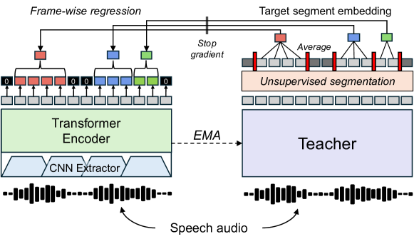
Figure 1: Overview of self-segmentation distillation. Sylber is trained with frame-wise regression on pseudo segment targets, obtained by an unsupervised segmentation algorithm on the teacher outputs.

Sylber is trained by a novel SSL framework, self-segmentation distillation, that imposes more explicit inductive bias of segment structure in feature representations by directly solving the speech segmentation problem. The diagram of our training process is depicted in Figure 1. Specifically, we use SDHuBERT (Cho et al., 2024b) as a starting point, and leverage its unsupervised syllable segments as pseudo targets of segmentation. The target segment labels are continuous embeddings averaged across frames within each segment that are found by an unsupervised segmentation algorithm. We use self-supervised knowledge distillation, where the teacher is an exponential moving average (EMA) of the student model (Grill et al., 2020; Caron et al., 2021; He et al., 2020). The target segment and segment embedding are extracted from the teacher, making the learning process self-supervised and free of labels. The loss objective is a frame-wise regression loss that minimizes the Mean Squared Error (MSE) between the output features at each frame and the target from the corresponding segment. Non-speech frames are regressed to zero. See Appendix A.1.1 for a formal definition.

Other than EMA, this learning objective is free of techniques that prevent collapse (e.g., contrastive learning, target recentering, masked prediction, etc). However, we find that initializing Sylber weights with SDHuBERT can avoid collapse even though a naive regression is highly vulnerable to collapse. Additionally, we include a denoising objective similar to Chen et al. (2022) to improve robustness of the model, where 20% of the batch inputs for the student are mixed with environmental noise (Reddy et al., 2021) or other speech audio. This additional denoising is not a primary source of learning as a syllabic structure is readily visible without it (Appendix A.1.7).

3.2 Linear time Greedy segmentation algorithm

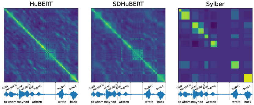
Figure 2: Frame-wise similarity matrix of raw features measured by dot product. For HuBERT and SDHuBERT, features from the ninth Transformer layer are extracted. As we can see, Sylber shows extremely salient syllabic structure that is aligned with the ground truth syllable boundaries.

The result of our self-segmentation distillation induces a framewise speech representation that exhibits a segmented structure as seen in the frame-wise similarity matrix (Figure 2, right). As we can see, our method produces a clean and robust segment structure that we can take advantage of to design a linear-time, greedy audio segmentation algorithm (also shown in Algorithm 1).

The algorithm involves three linear passes through the audio embeddings. The first step thresholds all of the embeddings by their L2 norm. This step allows us to differentiate between speech and non-speech segments. The second step is a monotonic agglomeration process where we sweep through each embedding and aggregate them into segments. Adjacent frames are merged together into a segment as long as their cosine similarity goes above a predefined merge threshold. This can be done in single pass without constructing the entire similarity matrix by greedily creating a new segment once a frame with a similarity below the threshold is seen.

The greedy segmentation algorithm can sometimes make some errors by shifting some frames, so a third pass is used to refine the boundaries of adjacent segments. For each boundary, a local search range is defined from the midpoint of the previous segment to the midpoint of the sub-sequence segment. From here, we can compute the cosine similarity between each frame and the averages of the two segments. For each candidate boundary in the search range, we compute an aggregate cosine similarity score between each frame and the assigned segment and maximize this sum to find the optimal boundary between adjacent segments.

Each one of these steps can be implemented with $O(n)$ complexity, so the entire segmentation algorithm has linear complexity with respect to the audio sequence length. As we can see in Table 1, this is significantly more efficient that previous segmentation approaches (Peng et al. (2023); Cho et al. (2024b); Komatsu & Shinozaki (2024)) which all have $O(n^{2})$ complexity.

4 Evaluating Categorical Perception in Speech Representation

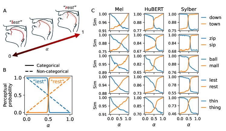
Figure 3: A. Overview of articulatory interpolation of rhyming words when interpolating $\alpha\in[0,1]$. B. Hypothetical curves of categorical (solid lines) and non-categorical (dashed lines) embeddings. C. Similarity curves examples from Melspectrogram (Mel), HuBERT layer 9, and Sylber. Sylber consistently shows highly categorical perception, drawing a sharp boundary in continuum between words.

Previous SSL-based tokens suffer from high redundancy in token vocabulary (Sicherman & Adi, 2023). This indicates that the SSL features densely tile the phonetic space without a clear boundary, resulting fine-grained, sub-phonemic units when clustered. Thus, to be better tokenized, the features should have distinct boundaries in their embedding space. This is well-aligned with categorical perception, a linguistic theory, which argues that human speech perception draws a categorical boundary in a continuum of speech sounds (Liberman et al., 1957; Pisoni & Lazarus, 1974; Harnad, 2003).

Inspired from this linguistic theory, we simulate interpolation between two rhyming words to probe the embeddings of speech SSL models to check whether they are categorical. Specifically, monosyllabic words are recruited where a single consonant is different at the front or back of the syllable (onset or coda). We make the contrast to be switching one of phonological properties: nasality, voicedness, or place (e.g., “b”all vs “m”all, “d”own vs ”t”own, or “l”est vs “r”est, respectively). We do not include vowel contrasts since categorical perception of vowels is not as consistent as consonants (Pisoni, 1973; Pisoni & Lazarus, 1974). We consider 13 types of such difference and simulate 4 pairs for each type, resulting 52 word pairs in total. The details of the difference types and the full list of word pairs can be found in Appendix A.4. To simulate a continuum between words, we utilize Articulatory Encodec (Cho et al., 2024c) which allows direct editing in the physical articulatory space (Figure 3-A). We first generate audio using the an off-the-shelf TTS API. We extract articulatory features from the speech, which are then temporally aligned by dynamic time warping to either end if necessary. We sample 51 equidistant samples in the linear interpolation between two words, where each end is manually adjusted to make the perceptual boundary drawn approximately in the middle ($\alpha=0.5$), which can be heard here. The pitch and loudness are also controlled to be at the same level. More details about Articulatory Encodec can be found in Section A.1.3.

Given a speech representation model, we extract features for each interpolating point between words in each pair. We calculate the similarity between interpolating features with features from either end, forming a likelihood curve along the interpolation. Hypothetically, if the representation is categorical, the likelihood curves should show a sharp transition at the boundary (Figure 3-B). If the embeddings are not categorical and tracing the interpolation, the curves would show “X” pattern as the dashed line in Figure 3-B. To quantify discriminability, we measure an empirical risk of wrong discrimination. Given words at the left and right ends in interpolation, $x_{L},x_{R}\in W$, the probability of being the left word given interpolating factor $\alpha$ is defined as $p(x_{L}|x_{\alpha})=\frac{\text{sim}(x_{L},x_{\alpha})-\text{offset}_{L}}{\text{sim}(x_{L},x_{\alpha})-\text{offset}_{L}+\text{sim}(x_{R},x_{\alpha})-\text{offset}_{R}}$. The probability of being the right word is symmetrically defined. We need to subtract an offset due to the high base similarity, as the words are rhyming pairs, such that $\text{offset}_{A}=\text{min}_{\alpha\in[0,1]}\text{sim}(x_{A},x_{\alpha})$. Then the empirical risk can be defined as $L_{\text{Disc}}(q|x_{L},x_{R}):=\mathbb{E}_{\alpha\in[0,1]}\mathbbm{1}_{\alpha<q}p(x_{R}|x_{\alpha})+\mathbbm{1}_{\alpha\geq q}p(x_{L}|x_{\alpha})$, for the decision boundary at $q\in[0,1]$. The optimal boundary can be drawn by minimizing the risk, $\alpha^{*}=\text{argmin}_{q\in[0,1]}L_{\text{Disc}}(q|x_{L},x_{R})$. Discriminability index (DI) is then defined as the risk at the optimal boundary, averaged over word pairs:

$$\text{DI}:=\frac{1}{|W|}\sum_{x_{L},x_{R}\in W}\>L_{\text{Disc}}(\alpha^{*}|x_{L},x_{R})$$ (1)

If the embeddings are categorical, DI will be close to 0. If they are non-categorical with X-shaped curves, DI will be 0.25. The maximum value of DI is 0.5, which would be random chance discrimination. This will be discussed later in §6.4 in detail.

5 Experimental Setup and evaluation protocol

5.1 Experimental Setup

Architecture Sylber has the same architecture as HuBERT with a CNN feature extractor followed by Transformer encoder. Based on the observation that the ninth layer of SDHuBERT best encodes syllables (Cho et al. (2024b)), we use a 9 layer transformer and initialize weights with SDHuBERT up-to that layer. See Appendix A.1.4 for training details.

Tokenization To tokenize speech, we apply the aforementioned segmentation algorithm (Section 3.2) to get unsupervised speech segments. The features within segments are averaged to form continuous speech tokens at a syllable granularity (4-5 syllables per second). We apply a simple k-means clustering on the features with several different vocab sizes (5K, 10K, and 20K). These cluster sizes are larger than what is used by other SSL-based clustering techniques (usually around 50-500 clusters), which is necessary since our features are more closer to syllables than phonemes; similar to how vocabulary sizes for BPE based tokenizers are significantly larger than the number of characters. However, these syllabic tokens have a significantly lower temporal resolution compared to previous SSL-based tokens, which leads to improvements to efficiency (see Section 6.2).

Token-to-speech If our syllabic tokens are valid speech tokens, we should be able to reconstruct intelligible speech from them. We train a Conditional Flow-matching (CFM) (Lipman et al., 2022; Le et al., 2024) model to generate low-level speech features that can be converted to speech audio. We utilize Articulatory Encodec (Cho et al., 2024c), an encoding-decoding framework that encodes speech into articulatory features and speaker identity, and decodes them back to speech waveform. The articulatory features are composed of spatiotemporal displacements of vocal tract articulators and source features that represent loudness and pitch. Cho et al. (2024c) empirically prove that these articulatory features are speaker agnostic provided that pitch is normalized, while allowing full-reconstruction to speech. We normalize pitch by dividing by speaker’s mean pitch and logscaling, following (Kharitonov et al., 2021). Since SSL-based speech tokens generally lack speaker information (Polyak et al., 2021; Wang et al., 2023), we aim to reconstruct these speaker-agnostic articulatory features from the syllabic tokens. The token embeddings are restored by the k-means codebooks, and expanded to the durations of the original segments. The non-speech frames are filled with zeros. For the case without quantization, the segment-averaged features are used. At inference time, we input the generated articulatory features with speaker embeddings extracted from original speech to the decoder of Articulatory Encodec to generate audio. See Appendix A.1.3 for the implementation and training details.

Unit LM Following Lakhotia et al. (2021), we train an autoregressive unit language model (uLM) using the syllabic tokens. The model has the same architecture as GSLM (Lakhotia et al., 2021), which is a decoder-only Transformer with 12 layers.

Datasets LibriSpeech (Panayotov et al., 2015) is used for pretraining Sylber, k-means clustering, and for training the uLMs. LibriTTS-R (Koizumi et al., 2023) is used for training the CFM models. For training Articulatory Encodec, we use an extended dataset that includes LibriTTS-R, LibriTTS (Zen et al., 2019), and EXPRESSO (Armougom et al., 2006).

5.2 Evaluation

Syllable detection and discovery We evaluate syllable boundaries with precision, recall, F1, and R-value with a 50 ms tolerance, following (Räsänen et al., 2009; Peng et al., 2023; Cho et al., 2024b; Komatsu & Shinozaki, 2024). Syllable discovery is evaluated by a separate clustering, where we use the same process as the previous works that use 4096 clusters. Then, we measure syllable purity, cluster purity, and mutual information between discovered syllables and ground truths (Cho et al., 2024b; Komatsu & Shinozaki, 2024). The same LibriSpeech dev/test sets are used as prior works.

Speech resynthesis We use the extracted speaker embedding and mean pitch from the original speaker to synthesize speech from articulatory features predicted from tokens. We use the original segment durations for each token without predicting them since the duration information can be easily tokenized. (For example, duration can be tagged for each token. See Appendix A.2.) We remove randomness in CFM to yield consistent generation for evaluation purposes. We measure reconstruction performance using the average Pearson Correlation of each component in articulatory features. To evaluate intelligibility, we use an off-the-shelf speech recognition model, Whisper (Radford et al., 2023), and measure word error rate (WER) and character error rate (CER). Lastly, we apply an automated speech quality measurement, UTMOS (Saeki et al., 2022), to evaluate the quality of generated speech. These are evaluated on the test-clean split of LibriTTS-R.

Coding efficiency We evaluate the coding efficiency of these tokens with Token/second (Tok/s), bitrate, and coding-rate. The bitrate is calculated by $(\text{log}_{2}(\text{vocab size}))\times\text{Tok/s}$. We define coding-rate as how much word information is preserved per bit: $\frac{(1-\text{WER}/100)\times\text{total \# of words}}{\text{total \# of bits}}$. Likewise, the test-clean split of LibriTTS-R is used.

Spoken Language Understanding (SLU) To evaluate the language understanding, we use the zero-shot metrics of lexical learning, sWUGGY, and syntax learning, sBLIMP, following Lakhotia et al. (2021); Algayres et al. (2023). These metrics are originally from the Zerospeech Challenge (Nguyen et al., 2020), for discriminating real words/phrases and fake ones. The tasks are solved zero-shot by choosing words/phrases with higher probability inferred by an LM and accuracy is reported.

Categorical perception For the models with frame-wise features, we use dynamic time warping to find an alignment that maximizes similarity. While some sample pairs are already aligned, we find that additional warping yields better scores. For models with syllabic features, we average across all speech (or norm thresholded) parts of the features as all samples are monosyllabic, yielding a single embedding per sample. We use cosine similarity to measure similarity between embeddings from samples, and evaluate DI as defined in §4.

5.2.1 Baselines

For syllable detection and discovery, we compare our models against HuBERT, VGHuBERT, SDHuBERT, and Komatsu & Shinozaki (2024). For token-to-speech, we train the baseline CFM models using HuBERT units with 50, 100, and 200 cluster sizes as used in Lakhotia et al. (2021), and SDHuBERT tokens with 5K, 10K, and 20K cluster sizes. For coding efficiency, we apply Byte Pair Encoding (BPE) using SentencePiece to merge frequent units to form larger vocabulary that matches ours: 5K, 10K, and 20K, similar to Shen et al. (2024). For evaluating language understanding, we use GSLM (Lakhotia et al., 2021) and tGSLM (Algayres et al., 2023) as baselines. We exclude other uLMs that use more extensive resources than ours (e.g., including a larger dataset or using a pretrained text-based LM.) However, we include tGSLM since it has a similar token granularity (5 Tok/s) as ours although it is trained on a 6$\times$ larger dataset. For phonetic discriminability, we compare Sylber with traditional acoustic features (Melspectrogram and MFCC), representative frame-wise SSL models (HuBERT, Wav2Vec2, and WavLM), and SDHuBERT. For frame-wise SSL models, the best layers with the lowest DIs are chosen.

6 Results

6.1 Syllable Detection and Discovery

Table 1: Syllable detection and discovery results. Pr: precision, Re: recall, R: R-value, SP: syllabic purity, CP: cluster purity, and MI: mutual information. Complexity indicates time complexity of post-hoc segmentation algorithm. $n$: the number of frames and $k$: the number of syllables. As we can see, only Sylber uses a linear time algorithm while the other models use a quadratic time algorithm.

Model	Complexity	Syllable Detection				Syllable Discovery
		Pr$\uparrow$	Re$\uparrow$	F1$\uparrow$	R$\uparrow$	SP$\uparrow$	CP$\uparrow$	MI$\uparrow$
HuBERT	$O(kn^{2})$	51.4	31.4	39.0	50.1	33.1	28.4	3.54
VGHuBERT	$O(kn^{2})$	65.3	64.3	64.8	70.0	53.4	43.6	4.66
SDHuBERT	$O(n^{2}/k)$	64.3	71.0	67.5	70.7	54.1	46.2	4.76
Komatsu & Shinozaki (2024)	$O(kn^{2})$	73.3	67.6	70.3	74.6	59.4	44.5	5.08
Sylber	$O(n)$	76.6	68.3	72.2	75.9	64.0	43.9	5.28

Table 1 shows a comparison of syllable detection and discovery performance. Sylber outperforms all previous approaches in every metric other than recall and cluster purity. As these two terms can be inflated by having more segments, it indicates that SDHuBERT is oversegmenting. In terms of discovery, we find the ground truth syllables are more purely mapped to ours than the baselines, greatly improving the previous SOTA by huge margin (59.4 $\rightarrow$ 64.0). The results indicate that our model can detect and discover syllables better than the previous approaches. Moreover, the output features from our model are significantly cleaner than HuBERT or SDHuBERT as shown in Figure 2, showing highly consistent similarities within syllable spans. This allows for a much faster $O(n)$ algorithm applicable, compared to the previous $O(kn^{2})$ and $O(n^{2}/k)$ algorithms where $n$ is the number of frames and $k$ is the estimate number of syllables controlled by a hyperparameter.

6.2 Resynthesis Performance and Coding Efficiency

Table 2: Resynthesis results. HB: HuBERT, SDHB: SDHuBERT, and KM: KMean cluster size. Reconstruction metrics are average Pearson Correlation and WER and CER are reported in percentage (%). 95% confidence interval is reported for reconstruction and quality. Best scores are highlighted with bold font and best scores with quantization are underlined.

Model		Reconstruction			Intelligibility		Quality	Frequency
Upstream	KM	Art$\uparrow$	Loudness$\uparrow$	Pitch$\uparrow$	WER$\downarrow$	CER$\downarrow$	UTMOS$\uparrow$	Tok/s$\downarrow$
HB	50	$0.926\pm 0.065$	$0.880\pm 0.089$	$0.586\pm 0.581$	13.32	7.24	$4.190\pm 0.553$	23.59
	100	$0.941\pm 0.046$	$0.878\pm 0.098$	$0.594\pm 0.560$	7.78	3.89	$4.177\pm 0.548$	26.68
	200	$\raisebox{-0.4pt}{\text@underline{\raisebox{0.4pt}{\smash{\text@underline{0.944}}}}}\pm\raisebox{-0.4pt}{\text@underline{\raisebox{0.4pt}{\smash{\text@underline{0.044}}}}}$	$\raisebox{-0.4pt}{\text@underline{\raisebox{0.4pt}{\smash{\text@underline{0.886}}}}}\pm\raisebox{-0.4pt}{\text@underline{\raisebox{0.4pt}{\smash{\text@underline{0.090}}}}}$	$0.608\pm 0.573$	6.34	3.10	$4.197\pm 0.543$	28.97
SDHB	5K	$0.925\pm 0.066$	$0.872\pm 0.089$	$0.757\pm 0.384$	9.88	5.40	$4.140\pm 0.660$	5.24
	10K	$0.927\pm 0.064$	$0.879\pm 0.083$	$0.759\pm 0.412$	9.25	4.99	$4.173\pm 0.600$
	20K	$0.930\pm 0.061$	$0.883\pm 0.081$	$\raisebox{-0.4pt}{\text@underline{\raisebox{0.4pt}{\smash{\text@underline{0.784}}}}}\pm\raisebox{-0.4pt}{\text@underline{\raisebox{0.4pt}{\smash{\text@underline{0.373}}}}}$	8.63	4.62	$4.180\pm 0.609$
	$\infty$	$\textbf{0.959}\pm\textbf{0.035}$	$0.948\pm 0.042$	$0.906\pm 0.217$	4.94	2.56	$4.190\pm 0.552$
Sylber	5K	$0.919\pm 0.072$	$0.877\pm 0.091$	$0.739\pm 0.431$	8.70	4.48	$4.189\pm 0.607$	4.27
	10K	$0.922\pm 0.064$	$0.876\pm 0.088$	$0.753\pm 0.424$	8.07	4.28	$4.155\pm 0.624$
	20K	$0.924\pm 0.066$	$0.882\pm 0.084$	$0.774\pm 0.374$	7.95	4.06	$\textbf{4.210}\pm\textbf{0.547}$
	$\infty$	$0.957\pm 0.037$	$\textbf{0.950}\pm\textbf{0.045}$	$\textbf{0.918}\pm\textbf{0.216}$	4.88	2.42	$4.199\pm 0.539$

The results of token-to-speech resynthesis are shown in Table 2 and can be heard here. We find a general trend in both SDHuBERT and our syllabic tokens that articulatory reconstruction and intelligibility increase with finer clustering granularity. For intelligibility, our model outperforms SDHuBERT at every vocab size while requiring less tokens per second. Interestingly, the articulatory reconstruction is generally higher in SDHuBERT, but also less intelligible. This indicates that our model marginalizes out some amount of articulatory variance which is orthogonal to orthographic contents. This marginalization is also happening in intonation when the embeddings are quantized, as shown in the huge reduction in pitch correlation compared to non-quantized model, resulting in a flattened speech generation. This pattern is shared in both SDHuBERT and our model.

Compared to HuBERT units which have token granularity at sub-phonemic level, the articulation is better reconstructed by HuBERT units with 200 clusters than the units from SDHuBERT or our model. This is natural given their temporal granularity as 28.97 tokens per second, which is likely to capture the local dynamics of articulation better than syllabic level. The intelligibility is also better in the case of 100 and 200 cluster sizes, WERs of 7.78 and 6.34, compared to the best case of syllabic units, WER of 7.95. Though the difference is marginal, HuBERT units require at least 6 times more tokens per second. Also, we find the HuBERT is worse in representing pitch, as suggested by Polyak et al. (2021); Kharitonov et al. (2021). While no significant difference is perceived in quality, our model with 20K vocab size quantization shows the best average UTMOS of 4.21.

Table 3: Coding efficiency comparison.

Model	Token/second$\downarrow$			Bitrate$\downarrow$			Coding-rate$\uparrow$
	Vocab size			Vocab size			Vocab size
	5K	10K	20K	5K	10K	20K	5K	10K	20K
HB50-BPE	7.45	6.82	6.30	91.57	90.68	90.00	0.0283	0.0285	0.0287
HB100-BPE	14.78	14.40	14.10	181.56	191.37	201.46	0.0152	0.0144	0.0137
HB200-BPE	16.67	15.99	15.53	204.79	212.41	221.84	0.0136	0.0132	0.0126
SDHB	5.24			64.39	69.63	74.87	0.0253	0.0243	0.0234
Sylber	4.27			52.43	56.70	60.97	0.0315	0.0302	0.0289

To better characterize coding efficiency, we compare bandwidth and coding-rate in Table 3 against baselines with comparable settings. Our model outperforms each baseline in every metric, showing about a 20% gain over the SDHuBERT tokens. In addition, Table 3 demonstrates the innate inefficiency in previous approaches using HuBERT units. There is a minimal gain in sequence compression while increasing the vocabulary size, where BPE is not able to reduce Tok/s by even half of the original when applied to 100 and 200 clusters. The only comparable baseline is BPE on 50 HuBERT clusters, which can reduce Tok/s from 23.59 to between 6.30 and 7.45. However, there is a huge information loss as shown in the high WER of 13.32, which results in a lower coding-rate (0.0283, 0.0285, 0.0287) compared to ours (0.0315, 0.0302, 0.0289) for vocab size of (5K, 10K, 20K) respectively. Without quantization, the best performance is achieved by our model, with a WER of 4.88, Tok/s of 4.27, and higher correlations in loudness and pitch (Table 2). This indicates the significant potential of syllabic tokens as an efficient speech coding that can be harnessed by a better quantization method like vector quantization (VQ) or residual VQ (RVQ), which we leave for future work.

6.3 Spoken Language Understanding (SLU)

Table 4: SLU Results

Model	sWUGGY$\uparrow$	sBLIMP$\uparrow$
GSLM	68.70	57.06
tGSLM	68.53	55.31
SDHB-5K	65.80	54.87
SDHB-10K	67.42	54.48
SDHB-20K	67.85	54.87
Sylber-5K	67.32	57.34
Sylber-10K	68.41	58.04
Sylber-20K	70.27	57.67

Table 4 compares the sWUGGY and sBLIMP scores of unit LMs with different vocab size of syllabic units (marked as “model-vocab size”), and the baseline models. Sylber with 20K vocab size outperforms GSLM and tGSLM in sWUGGY, and outperforms baselines at sBLIMP, while none of the SDHuBERT-based LMs outperform GSLM or tGSLM. This indicates that our syllabic tokens have better utility in terms of language modeling compared to the syllabic tokens from SDHuBERT. We also observe a general trend shared in SDHuBERT and ours that a larger vocab size yields a higher sWUGGY score, indicating a finer clustering better covers the lexical space. However, no such pattern was found in sBLIMP score. Notably, Sylber outperforms tGSLM which has a similar token granularity as 5 Hz but with a fixed pooling window, even though their model is trained on a larger dataset. This suggests that a variable pooling window which is dynamically driven by segmentation algorithm is better than using a fixed pooling window.

6.4 Demonstration of Emergent Categorical Perception

Table 5: Phonetic discriminability results. DI: Discriminability Index. Scores for different contrast postitions (onset, coda and all) are separately reported.

Model		DI$\downarrow$
		Onset	Coda	All
Acoustic	Mel	0.198	0.193	0.196
	MFCC	0.191	0.182	0.188
Frame-wise	Wav2Vec2	0.172	0.178	0.174
	HuBERT	0.136	0.152	0.141
	Wav2Vec2 Large	0.138	0.156	0.143
	HuBERT Large	0.166	0.180	0.170
	WavLM Large	0.136	0.148	0.140
Syllable-wise	SDHuBERT	0.133	0.126	0.131
	Sylber	0.116	0.103	0.112

Figure 3-C illustrates that a clear boundary is drawn when interpolating between two rhyming words, whereas such a boundary is less prominent in HuBERT. This indicates that Sylber needs only 2 categories to represent the interpolating continuum, while HuBERT requires multiple categories or units, which induces high level of inefficiency and redundancy in clustering (Sicherman & Adi, 2023). The curves extracted from the melspectrogram resemble an X-shape, indicating a non-categorical embedding space. This is the closest value to the hypothetical non-categorical score of 0.25 among the models (Table 5). As shown in Table 5, our model’s embeddings demonstrate the best discriminability, with the lowest DIs across both onset and coda contrasts, resulting in an overall DI of 0.112. SDHuBERT also shows lower DIs than frame-wise models, though it still falls short of our model’s performance. The results are highly surprising since we only impose the model to learn temporal structure, and our loss objective does not involve categorical learning at all. However, the embedding space of Sylber is naturally structured to be categorical, indicating the self-segmentation distillation might be a natural learning algorithm that resembles human language learning. Amongst the frame-wise models, WavLM-Large exhibits the best discriminability, which aligns with the fact that WavLM generally has superior representational power compared to other SSL models. Taken together, these qualitative and quantitative results suggest that the embedding space of Sylber is readily quantized, contributing to the performance improvements observed in previous sections.

7 Conclusion

We propose a novel self-supervised learning framework of speech that learns to transform speech waveform to syllabic embedding. As results, we achieve a state-of-the-art unsupervised syllable detection and discovery performance with a significant reduction in time complexity of segmentation algorithm, down to $O(n)$. The resynthesis experiments validate that our model can provide syllabic tokens that encodes intelligible speech content in highly efficient way. Up to our knowledge this is the first demonstration of speech synthesis from syllable-level tokens. Furthermore, a linguistic-theory inspired analysis reveals that Sylber also segments the embedding space, showing emergent categorical perception of speech. To sum, we introduce a new method for representing speech features as syllables, offering promising potential for more efficient speech tokenization and spoken language modeling.

Limitations Our model is not yet suitable for universal speech representation, which the most speech SSL approaches aim for (Yang et al., 2021). We find that Sylber degrades in some SUPERB downstream tasks, which we believe, is due to the parsimonious structure we are imposing (Appendix A.3). Furthermore, our model has not been scaled to a larger speech corpus, which may provide more gains than our current setting, as shown by previous studies (Borsos et al., 2022; Hassid et al., 2024). We leave these for future directions to explore.

Ethics Statement

We believe that Sylber is a substantial step forward for speech models and spoken language understanding. Our technique enables efficient and effective speech tokenization which can potentially be used for malicious purposes. It is important for users, researchers, and developers to use this model and this framework ethically and responsibly.

Reproducibility Statement

In the spirit of open research, we will be releasing all of the code associated with Sylber. We will release the pretrained model weights as well as the code necessary to retrain the model. In addition, we will be releasing all of the interpolation samples so that other researchers can also use our Discriminability Index as an evaluation metric for future research.

Appendix A Appendix

A.1 Implementation Details

A.1.1 Self-segmentation distillation

Given a speech audio, $x$, we extract features, $M_{S}(x)=z^{S}$ and $M_{T}(x)=z^{T}$, where $M_{S}$ and $M_{T}$ are the student and teacher models, respectively. The unsupervised segmentation algorithm, Useg, outputs segment boundaries from $z$ as $\text{Useg}(z)=\{s\}^{N}$, where $N$ is the number of discovered segments, and $s\in\mathbb{N}^{2}$ denotes start and end frames of the segment, indexed as $s_{j,0}$ and $s_{j,1}$ for the $j$-th segment. We define an assignment function, $A(i)=j$, that gives the index of the segment, $j$, given a frame number, $i$, such that $s_{j,0}\leq i<s_{j,1}$. When there is no assignable segment, $A(i)=-1$, meaning $i$ is a non-speech frame. The segment-averaged feature, $v_{j}$, is defined by averaging across frames in the $j$-th segment, $v_{j}=\frac{1}{p-q}\sum_{k\in[p,q]}z_{k}$, where $(p,q)=(s_{j,0},s_{j,1})$. Then, $v^{T}_{A(i)}$ indicates the teacher’s segment-averaged feature of the segment that $i$-th frame belongs to, being the target of the regression, which is zero for non-speech frame, $v^{T}_{-1}=0$. Finally, the loss function of the proposed self-segmentation distillation is defined as $\mathcal{L}_{\text{SegDistill}}:=\sum_{i}||v^{T}_{A(i)}-z^{S}_{i}||_{2}^{2}$.

Algorithm 1 Greedy Segmentation Algorithm

1:procedure Greedy-Segmentation(states, $N_{thr}$, $M_{thr}$)

2:     Compute L2 norms and mark speech frames: $\text{speech}_{i}=(\|s_{i}\|_{2}\geq N_{thr})$

3:     Initialize empty list of segments $S$

4:     for $i=1$ to $n$ do

5:         if $\text{speech}_{i}$ and (no current segment or $\text{sim}(s_{i},s_{i-1})<M_{thr}$) then

6:              Start new segment $S_{k+1}$ with $s_{i}$

7:         else if $\text{speech}_{i}$ then

8:              Add $s_{i}$ to current segment $S_{k}$

9:         else if current segment $S_{k}$ exists then

10:              Finalize current segment $S_{k}$

11:         end if

12:     end for

13:     for each boundary $j$ between segments $S_{k}$ and $S_{k+1}$ do

14:         if $\text{speech}_{j}$ then

15:              Define local search range from $a=\text{midpoint}(S_{k})$ to $b=\text{midpoint}(S_{k+1})$

16:              Find optimal boundary $j^{*}$ = $\operatorname*{arg\,max}_{j}\sum_{i=a}^{j}\text{sim}(s_{i},\text{avg}(S_{k}))+\sum_{i=j+1}^{b}\text{sim}(s_{i},\text{avg}(S_{k+1}))$

17:              Update boundary to $j^{*}$

18:         end if

19:     end for

20:     return $S$

21:end procedure

A.1.2 Noise Augmentation

For denoising objective, we mix the input with a randomly sampled environmental sound or other speech audio. For mixing with environmental sound, we randomly select a clip from Reddy et al. (2021) and sample a 5 seconds clip from it. We first z-score the waveform and multiply by a factor sampled from $[0.05,0.7]$, and mix with original speech audio. Note that the original speech is also z-scored. For mixing with other speech, we randomly select another clip in the batch and shift from left or right with a percentage sampled from $[0.4,0.7]$, to make sure the original speech holds the dominant information context in the mixture. The magnitude is also modulated by multiplying by a factor sampled from $[0.0,0.2]$. We apply this augmentation to 20% of the samples in the batch, and only to the inputs fed to the student model. Within the 20%, we have the source of noise be 75% environmental noise and 25% other speech.

A.1.3 Token-to-speech

Articulatory Encodec Articulatory Encodec (Cho et al., 2024c) is composed of articulatory encoding and decoding. The encoding pipeline outputs 14 articulatory features at 50 Hz are used, which are composed of the XY coordinates of 6 articulators (lower incisor; upper and lower lips; tongue tip, blade and dorsum;), and loudness and pitch. These are interpretable and grounded representations of speech that are fully informative of speech contents (Cho et al., 2024c). The decoder, or articulatory vocoder, is a Hifi-GAN (Kong et al., 2020) conditioned on a speaker embedding inferred from a separate speaker encoder. Cho et al. (2024c) shows that Articulatory Encodec successfully decomposes speech contents and speaker identity, by normalizing pitch to remove speaker specific pitch level. We replicate the implementation from Cho et al. (2024c), except that we change the layer of WavLM from which speaker information is extracted from the CNN outputs to the sixth Transformer layer, based on the observation that this layer contributes the most to the downstream speaker identification task (Chen et al., 2022).

Conditional flow-matching (CFM) The input model in the CFM is composed of two feed forward networks (FFNs) and a linear layer, where each FFN has two linear layers with 512 hidden units and residual connection, with a ReLU activation and dropout rate of 0.05. Also, Layernorm is applied to the output of each FFN. The final linear layer projects the 512 dimensional feature to 256. The Transformer in the CFM has 8 layers and each layer has 8 heads with 64 dimensions, and 512 for the encoding dimension. We use Rotary positional embeddings (Su et al., 2024). The final output is projected to the 14 dimensional flow in articulatory feature space.

A.1.4 Training Details

We train Sylber in two stages. The first stage is training with segment boundaries inferred from SDHuBERT which are extracted once at the beginning and fixed while in this stage. The second stage utilizes online segmentation using the teacher model’s outputs, by the algorithm in §3.2. Note that this training is only possible since our model exhibits features clean enough for our greedy segmentation to work. In the second stage, the L2 norm threshold is updated online by aggregating the statistics of speech and non-speech segments, and the merge threshold is randomly sampled from $[0.8,0.9]$. After the training, the norm threshold is fixed at 3.09 and the merge threshold is fixed at 0.8. See Appendix A.1.5 for details about the thresholding. Sylber is trained for 1.15M steps in the first stage and further trained for 500k steps in the second stage. We use a batch size of 64 and each data point is randomly cropped to be 5 seconds, following Cho et al. (2024b). The learning rate is set as 1e-4 with initial 500 warmup updates for the first stage and 5e-5 for the second stage. The EMA decay rates are set as 0.9995 and 0.9999 for the first and second stages, respectively. The second stage training improves performance in syllable detection and discovery (Appendix A.1.6).

For the CFM, the learning rate is fixed as 1e-4, with a batch size of 64 and 200k updates. For Articulatory Encodec and unit LM, we largely follow Cho et al. (2024c) and Lakhotia et al. (2021), respectively.

A.1.5 Thresholds Setting

Thresholds in SDHuBERT segmentation For segmentation on SDHuBERT features, we apply the minimum cut algorithm introduced by Peng et al. (2023) and modified by Cho et al. (2024b). Following Cho et al. (2024b), the initial mask is obtained by thresholding norms of features from the eleventh layer of Transformer, where we normalize norms to be in $[0,1]$ and use 0.1 as threshold. The minimum cut refines each masked chunk to make it syllabic. Specifically, the algorithm conducts within segment agglomerative clustering with a preset number of clusters. This preset number is estimated by a pre-defined speaking rate. As this preset number of syllables may be larger than the number of segments, a post-hoc merging process merges adjacent segments with cosine similarity higher than a threshold, which we call the merge threshold. For tokenization experiments, we use a more sensitive segmentation configuration than the original setting to prevent loss of speech contents due to overly broad segments. Specifically, we halve the estimated syllable duration from 200ms to 100ms to cover speech with fast speaking rate, and increase the merge threshold from 0.3 to 0.4. However, the SDHuBERT is still sensitive to non-speech noise events. Therefore, we filter out segments with average absolute amplitude of waveform lower than 0.05

Thresholds in Sylber greedy segmentation algorithm Unlike the thresholds in SDHuBERT, which are heuristically driven, we try to set the thresholds in our algorithm more principled way, especially in the second stage of training where the target segments are dynamically generated. We first set the norm threshold to be optimal boundary between signal (speech) and noise (non-speech), where the likelihoods of being signal and noise are equal. We assume both signal and noise distributions to be Gaussian and solve the equality condition. After the first training stage, we use the pseudo ground truth segments used for training to get the distribution of segment norms and non-segment norms in the dev split of LibriSpeech. To make the distribution reflects noise, we apply the noise augmentation as described in the denoising objective (Sec. A.1.2) to each sample. In the second training stage, we update the mean and variance of noise distribution using the non-segment portions of student outputs using an exponential moving average with a decay rate of 0.9999, while keeping the signal distribution the same as initially set. This results in the threshold of 3.09 after training. While these segments may not require such frequent updates in threshold, we implement this to try to keep it principled and empirically driven.

On the other hand, we still remain largely heuristically driven in terms of setting our merge threshold. We use a particularly high threshold of 0.8 compared to 0.3 in the previous works. Such a high threshold for merging is effective in Sylber since the features are much cleaner than SDHuBERT. Instead setting this threshold to a fixed number, we sample a value from $[0.8,0.9]$ during the second stage training, which is somewhat arbitrarily set after visually inspecting multiple samples. We found that 0.7 also generally works fine but we select 0.8 as the threshold for the inference since that is the lowest number in the range we impose during training. In fact, the phoneme recognition experiment empirically proves that 0.8 is optimal when thresholds of 0.1 increments are tested (Table 8).

A.1.6 Effect of The Second Stage Training with Online Segmentation

To check the effectiveness of the second stage training with the online segmentation, we compare syllable detection and discovery metrics between the stage 1 and stage 2 models. As shown in Table 6, we observe some gain after the second stage training, especially in precision of the segmentation.

Table 6: Syllable detection and discovery performance comparison between two stages.

Model	Syllable Detection				Syllable Discovery
	Pr$\uparrow$	Re$\uparrow$	F1$\uparrow$	R$\uparrow$	SP$\uparrow$	CP$\uparrow$	MI$\uparrow$
Sylber-Stage-1	73.7	69.2	71.4	75.6	63.2	43.9	5.24
Sylber-Stage-2	76.6	68.3	72.2	75.9	64.0	43.9	5.28

A.1.7 Effect of Denoising Objective

As demonstrated in left two panels in Figure 4, the syllabic structures are already highly visible without the denoising objective, indicating that the major learning source is self-segmentation distillation than the denoising objective. However, adding the denoising objective significantly improves robustness; otherwise, the model becomes highly sensitive to noisy audio as shown in the right two panels in Figure 4.

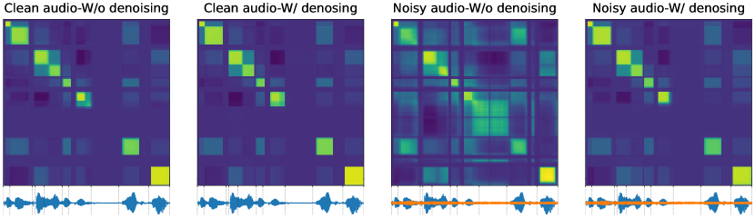
Figure 4: Frame-wise similarity matrix from with and without denosing objectives, using clean signal (left two panels) and noisy signal (right two panel). The orange waveform depicts the source noise we add to the clean speech signal.

A.2 Coding Efficiency with Duration-informed Tokenization

When we measure coding efficiency in §2, we ignore the duration information. Here, we recalculate the metrics by adding duration as separate token tagged to each speech token. Note that duration is counted as the number of frames, so it already lies on discrete space. We find that 99% of HuBERT tokens have duration less than 8, 7, and 6 with the vocab size of 50, 100, and 200, respectively. This means that the duration of each token can be coded by 3 bits. However, when BPE is applied, these 3 bits will be multiplied by the maximum number of units in subwords to count per-token duration bits, which is 10 to 16 depending on the vocab size and cluster granularity.

The syllabic tokens do not densely cover the frames. Therefore, the duration of subsequent silence can be tagged along with the duration of the tokens. 98% of syllabic tokens have duration less than or equal to 16 (4 bits). We can also keep the subsequent silence duration up-to 7 frames (3 bits) efficiently, and silence longer than 7 frames can be regarded as a separate “silence token”, adding one more token to the k-means codebook.

Taking all these into consideration, we measure the coding efficiency metrics with the duration-informed tokens as Table 7. Compared to Table 3, the gap between HuBERT-BPE and ours gets even larger, where we achieve around or more than $4\times$ gains compared to HuBERT baselines. Moreover, even after appending duration tokens, we achieve significantly lower bitrates which are below or around 100.

Table 7: Coding efficiency of duration-informed tokens.

Model	Token/second$\downarrow$			Bitrate$\downarrow$			Coding-rate$\uparrow$
	Vocab size			Vocab size			Vocab size
	5K	10K	20K	5K	10K	20K	5K	10K	20K
HB50-BPE	7.45	6.82	6.30	449.26	418.24	392.36	0.0058	0.0062	0.0066
HB100-BPE	14.78	14.40	14.10	624.82	666.64	709.06	0.0044	0.0041	0.0039
HB200-BPE	16.67	15.99	15.53	654.77	979.72	967.13	0.0043	0.0029	0.0029
SDHB	5.84			112.73	118.58	124.42	0.0239	0.0228	0.0219
Sylber	4.76			91.80	96.56	101.32	0.0297	0.0284	0.0271

A.3 General Representational Power of Sylber

Though the universal utility of our model is not of our focus, we evaluate and benchmark downstream tasks using SUPERB (Yang et al., 2021). First of all, to find the optimal merge threshold, we train a phoneme recognition (PR) model with syllabic embeddings, where the merge threshold is sampled from $[0.3,0.9]$. The regular CTC based approach is not applicable to syllabic granularity, since it requires that the input length must be no shorter than the target length. Instead, we adopt RNN-T (Graves, 2012) which has no restriction on sequence length. To keep the model size similar to the PR model in SUPERB, we use a very simple, non-RNN transcriber, which is a Layernorm followed by two linear layers where the GELU activation function is applied to the first linear layer’s output. The output size of the first layer is set as 768 and set as the vocab size of phonemes, 73, for the second layer. The predictor network has a 3 layer LSTM with a hidden size of 1024, 0.1 dropout rate and Layernorm applied. The model is trained with the RNN-T implementation in PyTorch, and we use beam size of 5 for decoding. The learning rate is set as 0.001 and AdamW is used. The model is trained until no improvement is found in validation loss. We use LibriSpeech clean subsets (train-clean, dev-clean, and test-clean), which is the dataset used in SUPERB PR task setting. As results in Table 8, the merge threshold of 0.8 is selected and used throughout the SUPERB evaluation. This number coincides with the threshold we use in the main results as well. We use the code provided by S3PRL for the experiment.

Table 8: Phoneme recognition on LibriSpeech (LS) dev-celan with different merge threshods.

Dataset	PER $\downarrow$
	Mthr=0.5	Mthr=0.6	Mthr=0.7	Mthr=0.8	Mthr=0.9
LS dev-clean	6.15	5.88	5.73	5.68	5.68

We evaluate 3 versions of Sylber. We freeze the model following the SUPERB protocol.

Sylber-All Layer uses all layer features without segmenting with 50 Hz full-sampling rate, being a regular entry to SUPERB.
Sylber-Segment uses segment embedding after segmentation, with syllable granularity.
Sylber-Segment-Expand expands segment embedding to original length.

Table 9 compares these with a HuBERT base model, which has a comparable model size and trained on the same data. Since Sylber-Segment has a shorter sequence length than the target, thus making the CTC-based recognition task inapplicable, we replace the scores using the aforementioned RNN-T model, and we find a reasonable performance in PR as PER of 5.98, while ASR is lagging by large margin. As our model features are syllabic, this structure may need to be resolved to be converted to characters, adding additional layer of complexity than mapping phonemic features to characters which is hard to resolve in a limited resource setting.

Another notable point is that our models achieve higher keyword spotting accuracy (KS) and intent classification (IC) compared to the HuBERT base model in all 3 versions. This is aligned with the improved performance in language learning reported in §6.3. Also, there is a huge drop in speaker identity accuracy (SID) when our syllabic embedding is used, indicating that the speaker information is somewhat marginalized out.

Also, the failure in slot filling (SF) and automatic speech verification (ASV) by Sylber-Segment is attributed to the fact that S3PRL is tuned to lengthy input of speech representation with a regular sampling rate. Further investigation is required, for a proper application of syllabic embedding to those tasks.

Table 9: Performance comparison of various models across different metrics

Model	PR	KS	IC	SID	ER	ASR	ASR (w/ LM)	QbE	SF		ASV	SD
	PER$\downarrow$	Acc$\uparrow$	Acc$\uparrow$	Acc$\uparrow$	Acc$\uparrow$	WER$\downarrow$	WER$\downarrow$	MTWV $\uparrow$	F1$\uparrow$	CER$\downarrow$	EER$\downarrow$	DER$\downarrow$
Hubert-base	5.41	96.3	98.34	81.42	64.92	6.42	4.79	0.0736	88.53	25.2	5.11	5.88
Sylber-All Layer	11.78	96.75	98.44	76.16	64.34	11.76	8.32	0.0623	85.79	29.21	6.72	5.08
Sylber-Segment	∗5.98	97.08	98.92	50.59	64.50	∗14.07	–	0.0139	–	–	–	13.21
Sylber-Segment-Expand	88.79	97.11	99.08	51.25	65.25	12.04	8.88	0.0591	85.66	29.49	8.75	15.55

A.4 Rhyming Word Pairs

For the consonant at the onset, we constrain the difference to be phonologically adjacent: voiced or voiceless sounds (e.g., “d”own vs ”t”own), non-nasal or nasal sounds (e.g., “b”all vs “m”all), or spatially adjacent pairs (e.g., “l”est vs “r”est). For the consonant at the coda, we confine the words to have “/I/” at the nucleus vowel to minimize different coarticulation pattern induced by different ending consonants. We only consider nasality difference at the coda and we regard voiced and unvoiced consonants the same since voiced-ness is relatively subtle at the coda position. Additionally, we include “n-ng” contrast. Table 10 shows the full list of word pairs.

Table 10: Rhyming word pairs used in the discriminability task.

Onset
Voicedness
b-p	v-f	d-t	z-s	g-k
bay, pay	vill, fill	down, town	zeal, seal	goal, coal
bar, par	vine, fine	dall, tall	zip, sip	gap, cap
ban, pan	vault, fault	deen, teen	zig, sig	gain, cane
bad, pad	vox, fox	dime, time	zoo, sue	gauge, cage
Nasality		Place
b-m	d-n	l-r	t-s
ball, mall	dose, nose	lock, rock	tank, sank
bean, mean	dull, null	lane, rain	tale, sale
boon, moon	dine, nine	long, wrong	tip, sip
bost, most	deal, kneal	lest, rest	tell, sell
Coda
g/k-ng	n-ng	d/t-n	b/p-m
pig, ping	thin, thing	kid, kin	trip, trim
sick, sing	bin, bing	seed, seen	deep, deem
dig, ding	sin, sing	chit, chin	sip, seem
click, cling	kin, king	grid, grin	rip, rim

References

- Abdullah et al. (2023) Badr M Abdullah, Mohammed Maqsood Shaik, Bernd Möbius, and Dietrich Klakow. An information-theoretic analysis of self-supervised discrete representations of speech. arXiv preprint arXiv:2306.02405, 2023.
- Algayres et al. (2023) Robin Algayres, Yossi Adi, Tu Anh Nguyen, Jade Copet, Gabriel Synnaeve, Benoit Sagot, and Emmanuel Dupoux. Generative spoken language model based on continuous word-sized audio tokens. arXiv preprint arXiv:2310.05224, 2023.
- Armougom et al. (2006) Fabrice Armougom, Sebastien Moretti, Olivier Poirot, Stephane Audic, Pierre Dumas, Basile Schaeli, Vladimir Keduas, and Cedric Notredame. Expresso: automatic incorporation of structural information in multiple sequence alignments using 3d-coffee. Nucleic acids research, 34(suppl_2):W604–W608, 2006.
- Baevski et al. (2020) Alexei Baevski, Yuhao Zhou, Abdelrahman Mohamed, and Michael Auli. wav2vec 2.0: A framework for self-supervised learning of speech representations. Advances in neural information processing systems, 33:12449–12460, 2020.
- Baevski et al. (2021) Alexei Baevski, Wei-Ning Hsu, Alexis Conneau, and Michael Auli. Unsupervised speech recognition. Advances in Neural Information Processing Systems, 34:27826–27839, 2021.
- Borsos et al. (2022) Zalán Borsos, Raphaël Marinier, Damien Vincent, Eugene Kharitonov, Olivier Pietquin, Matt Sharifi, Olivier Teboul, David Grangier, Marco Tagliasacchi, and Neil Zeghidour. Audiolm: a language modeling approach to audio generation.(2022). arXiv preprint arXiv:2209.03143, 2022.
- Caron et al. (2021) Mathilde Caron, Hugo Touvron, Ishan Misra, Hervé Jégou, Julien Mairal, Piotr Bojanowski, and Armand Joulin. Emerging properties in self-supervised vision transformers. In Proceedings of the IEEE/CVF international conference on computer vision, pp. 9650–9660, 2021.
- Chang et al. (2024) Xuankai Chang, Brian Yan, Kwanghee Choi, Jee-Weon Jung, Yichen Lu, Soumi Maiti, Roshan Sharma, Jiatong Shi, Jinchuan Tian, Shinji Watanabe, et al. Exploring speech recognition, translation, and understanding with discrete speech units: A comparative study. In ICASSP 2024-2024 IEEE International Conference on Acoustics, Speech and Signal Processing (ICASSP), pp. 11481–11485. IEEE, 2024.
- Chen et al. (2022) Sanyuan Chen, Chengyi Wang, Zhengyang Chen, Yu Wu, Shujie Liu, Zhuo Chen, Jinyu Li, Naoyuki Kanda, Takuya Yoshioka, Xiong Xiao, et al. Wavlm: Large-scale self-supervised pre-training for full stack speech processing. IEEE Journal of Selected Topics in Signal Processing, 16(6):1505–1518, 2022.
- Cho et al. (2023) Cheol Jun Cho, Peter Wu, Abdelrahman Mohamed, and Gopala K Anumanchipalli. Evidence of vocal tract articulation in self-supervised learning of speech. In ICASSP 2023-2023 IEEE International Conference on Acoustics, Speech and Signal Processing (ICASSP), pp. 1–5. IEEE, 2023.
- Cho et al. (2024a) Cheol Jun Cho, Abdelrahman Mohamed, Alan W Black, and Gopala K Anumanchipalli. Self-supervised models of speech infer universal articulatory kinematics. In ICASSP 2024-2024 IEEE International Conference on Acoustics, Speech and Signal Processing (ICASSP), pp. 12061–12065. IEEE, 2024a.
- Cho et al. (2024b) Cheol Jun Cho, Abdelrahman Mohamed, Shang-Wen Li, Alan W Black, and Gopala K Anumanchipalli. Sd-hubert: Sentence-level self-distillation induces syllabic organization in hubert. In ICASSP 2024-2024 IEEE International Conference on Acoustics, Speech and Signal Processing (ICASSP), pp. 12076–12080. IEEE, 2024b.
- Cho et al. (2024c) Cheol Jun Cho, Peter Wu, Tejas S Prabhune, Dhruv Agarwal, and Gopala K Anumanchipalli. Articulatory encodec: Vocal tract kinematics as a codec for speech. arXiv preprint arXiv:2406.12998, 2024c.
- Choi et al. (2024) Kwanghee Choi, Ankita Pasad, Tomohiko Nakamura, Satoru Fukayama, Karen Livescu, and Shinji Watanabe. Self-supervised speech representations are more phonetic than semantic. arXiv preprint arXiv:2406.08619, 2024.
- Chung et al. (2021) Yu-An Chung, Yu Zhang, Wei Han, Chung-Cheng Chiu, James Qin, Ruoming Pang, and Yonghui Wu. W2v-bert: Combining contrastive learning and masked language modeling for self-supervised speech pre-training. In 2021 IEEE Automatic Speech Recognition and Understanding Workshop (ASRU), pp. 244–250. IEEE, 2021.
- Gong et al. (2023) Xue L Gong, Alexander G Huth, Fatma Deniz, Keith Johnson, Jack L Gallant, and Frédéric E Theunissen. Phonemic segmentation of narrative speech in human cerebral cortex. Nature communications, 14(1):4309, 2023.
- Graves (2012) Alex Graves. Sequence transduction with recurrent neural networks. arXiv preprint arXiv:1211.3711, 2012.
- Greenberg (1998) Steven Greenberg. A syllable-centric framework for the evolution of spoken language. Behavioral and brain sciences, 21(4):518–518, 1998.
- Grill et al. (2020) Jean-Bastien Grill, Florian Strub, Florent Altché, Corentin Tallec, Pierre Richemond, Elena Buchatskaya, Carl Doersch, Bernardo Avila Pires, Zhaohan Guo, Mohammad Gheshlaghi Azar, et al. Bootstrap your own latent-a new approach to self-supervised learning. Advances in neural information processing systems, 33:21271–21284, 2020.
- Hallap et al. (2022) Mark Hallap, Emmanuel Dupoux, and Ewan Dunbar. Evaluating context-invariance in unsupervised speech representations. arXiv preprint arXiv:2210.15775, 2022.
- Harnad (2003) Stevan Harnad. Categorical perception. 2003.
- Hassid et al. (2024) Michael Hassid, Tal Remez, Tu Anh Nguyen, Itai Gat, Alexis Conneau, Felix Kreuk, Jade Copet, Alexandre Defossez, Gabriel Synnaeve, Emmanuel Dupoux, et al. Textually pretrained speech language models. Advances in Neural Information Processing Systems, 36, 2024.
- He et al. (2020) Kaiming He, Haoqi Fan, Yuxin Wu, Saining Xie, and Ross Girshick. Momentum contrast for unsupervised visual representation learning. In Proceedings of the IEEE/CVF conference on computer vision and pattern recognition, pp. 9729–9738, 2020.
- Hsu et al. (2021) Wei-Ning Hsu, Benjamin Bolte, Yao-Hung Hubert Tsai, Kushal Lakhotia, Ruslan Salakhutdinov, and Abdelrahman Mohamed. Hubert: Self-supervised speech representation learning by masked prediction of hidden units. IEEE/ACM transactions on audio, speech, and language processing, 29:3451–3460, 2021.
- Hu et al. (2024) Shujie Hu, Long Zhou, Shujie Liu, Sanyuan Chen, Hongkun Hao, Jing Pan, Xunying Liu, Jinyu Li, Sunit Sivasankaran, Linquan Liu, et al. Wavllm: Towards robust and adaptive speech large language model. arXiv preprint arXiv:2404.00656, 2024.
- Kharitonov et al. (2021) Eugene Kharitonov, Ann Lee, Adam Polyak, Yossi Adi, Jade Copet, Kushal Lakhotia, Tu-Anh Nguyen, Morgane Rivière, Abdelrahman Mohamed, Emmanuel Dupoux, et al. Text-free prosody-aware generative spoken language modeling. arXiv preprint arXiv:2109.03264, 2021.
- Koizumi et al. (2023) Yuma Koizumi, Heiga Zen, Shigeki Karita, Yifan Ding, Kohei Yatabe, Nobuyuki Morioka, Michiel Bacchiani, Yu Zhang, Wei Han, and Ankur Bapna. Libritts-r: A restored multi-speaker text-to-speech corpus. arXiv preprint arXiv:2305.18802, 2023.