Classification of Buried Objects from Ground Penetrating Radar Images by using Second Order Deep Learning Models

Abstract

In this paper, a new classification model based on covariance matrices is built in order to classify buried objects. The inputs of the proposed models are the hyperbola thumbnails obtained with a classical Ground Penetrating Radar (GPR) system. These thumbnails are entered in the first layers of a classical CNN which results in a covariance matrix by using the outputs of the convolutional filters. Next, the covariance matrix is given to a network composed of specific layers to classify Symmetric Positive Definite (SPD) matrices. We show in a large database that our approach outperform shallow networks designed for GPR data and conventional CNNs typically used in computer vision applications, particularly when the number of training data decreases and in the presence of mislabeled data. We also illustrate the interest of our models when training data and test sets are obtained from different weather modes or considerations.

I Introduction

The Ground Penetrated Radar (GPR) is a RADAR system that provides an image of the underground [1, 2, 3]. In particular, it can be used to image buried objects such as mines, pipes (metal, plastic, cast iron, etc.) and even cavities. The main drawback of GPR images is that they are very noisy, in particular due to the clutter that is the sum of all contributions from micro-scatterers in the ground but also because of the strong answer of the different layers of the ground. It is therefore often difficult to detect/locate buried objects, and even more so to classify them. One solution is to use complex systems such as stepped frequency RADAR [4], Multiple Input Multiple Output (MIMO) [5], or polarimetric sensors. But the high cost of these devices is not always attractive for industrial or civil engineering applications. In this paper, we consider classical GPR systems emitting a single wave, called Ricker, and whose image is created by a displacement on one axis of the transmitting/receiving system. In the normal configuration, the RADAR is positioned very close to the ground. In our case, we will study the possibility of placing the RADAR at a certain height above the ground. This study will enable us to assess the robustness of our approach in the case of using GPR placed on a drone.

As noticed previously, the bad quality of the GPR image requires the use of various signal processing, image processing or machine learning techniques to achieve just the right detection and localization performance. In machine learning, it is possible to use deep learning techniques for denoising or inversion [6, 7, 8, 9], auto-encoders for detection [10] or pattern recognition approaches for localization of buried objects [11]. In signal processing, it is possible to use statistical methods normally used in detection [12, 13, 14, 15], particle filtering [16], Markov fields [17] or algebraic algorithms [18, 19]. In image processing, most of methods are based on inversion [20, 21], compressive sensing [22] or dictionary learning [23]. A robust inversion method has been proposed in [24], which achieves good performance whatever the type of soil or buried object. All these works are essential for good object detection and localization, but will not suffice if we wish to classify them and thus determine their physical properties. In this paper, we are interested in this last step. Before introducing the proposed approach, we give the different assumptions: firstly all the buried objects are detected and correctly localized and secondly we have a certain amount of training data at our disposal, enabling us to develop supervised approaches.

For the classification of buried objects from GPR images, a number of studies already exist, based either on classical signal processing techniques [25, 26], machine learning [27, 28] or deep networks [29, 30, 31, 32]. In all these algorithms, detection is based on the shape of the hyperbola (in both axes), which is partly related to the shape of the buried object and its electromagnetic properties. Unfortunately, the shape of the hyperbola also depends on elements completely independent of the object. In particular, the technical characteristics of the GPR (frequency, elevation) as well as the type of soil and the number of layers between the object and the ground have an enormous influence on this shape. The aim of this paper is to propose a high-performance approach that will remain effective in as many experimental configurations as possible. To address this problem, it seems obvious to turn to deep network techniques. However, it is not obvious that the desired robustness can be achieved, particularly if only a small amount of training data is available. Indeed, in this case, it is prudent to create shallow deep learning models that work well with little training data. Unfortunately, this type of model is not known to be very robust, as it cannot take into account the full richness of the data. In the case of a deep network that might have this feature, the concern is that the small amount of training data is likely to lead to mixed performance.

One solution is then to change of features before the classification step. Instead of the image of the hyperbola, a suitable transformation can achieve the performance and robustness objectives sought in this study. For example, it is possible to construct a covariance matrix from this image by using the method proposed in [33]. It is known that second order can improve classification performance, as for example in computer vision [34, 35]. Moreover, we have shown in [36] that this kind of feature brings robustness when a shift is present between the training and the test data. By using a similar approach of [33], we have shown in a previous work [37] that this operation achieves better performance with classical machine learning algorithms than using the raw image. This covariance matrix is constructed from the outputs of the first layers of a deep network. It measures the correlations between these different layers for a given image. To achieve a certain richness in this covariance matrix, it is often useful to use a certain number of layers (around 8-10). In this case, however, the covariance matrix is very large, making classification impossible caused by singularities issues. To solve this issue, a preliminary work [38] has proposed specific layers for Symmetric Positive Definite (SPD) matrices, properties of covariance matrices, to solve this problem of classifying from large covariance matrices. Similar models have also been proposed for EEG data analysis [39], classification of RADAR data [40] or classification in polarimetric SAR images [41].

In this paper, we propose a new classification model based on a transformation of the raw image into a covariance matrix and specific subsequent layers adapted to this SPD matrix. We also propose a different approach to that proposed in [33] for constructing our covariance matrix, which saves memory space while preserving correlation information. To train and test our new model, we have from Geolithe, a sufficient database containing 4 types of buried objects with different GPR configurations (frequency and elevation) as well as several terrains (dry and wet sand and gravel). We compare our approach with shallow networks and conventional deep networks used in computer vision. We will show good performance and, above all, robustness of our pipeline to different experiments.

The outline of the paper is the following. First, section II introduces the GPR principle as well as some physical considerations allowing to better understand how the shape of the hyperbolas and the buried object are linked. Section III presents the new model to classify buried objects from GPR images. Next, section IV gives some details on the used database for the training and the steps. Finally, our approach is tested and compared to other algorithms in the section V.

II Ground Penetrating Radar (GPR)

II-A GPR Principle

Ground Penetrating Radar (GPR) is a radar system consisting of an antenna that is typically placed on the surface of the ground. For a wide range of systems, the electromagnetic wave transmitted by the GPR is a simple wavelet, known in the community as a Ricker. An example of this type of signal is shown in figure 1. The frequency of the wave, from 10MHz to 2GHz, depends on the application. In fact, this frequency is linked to the depth that can be reached. For example, for mine detection, a high frequency will be chosen, as there is no need to reach great depths, whereas the opposite will be chosen if you want to know the composition of the ground over several tens of meters.

Figure 1: Waveform emitted by classical GPR, called Ricker.

The GPR is moved along an axis, as shown on the left of the figure 2. All acquisitions, i.e. the amplitude of the signal over time at a given point, are combined to form an image known as the A-scan. From this A-scan, it is then possible to construct an image of the ground called a B-scan or radargram. All processing, from detection to classification, is classically based on this image. If a buried object is present, it is then seen several times by the GPR, leading to a hyperbola in the B-scan image. Soils are often composed of several layers of different types. In this case, the B-scan shows some lines to represent these layers. On the right-hand side of the figure, the B-scan shows the image of a buried object and two layers. In this simple simulation, we do not take noise into account. In reality, the signal-to-noise ratio of GPR images is very low. In particular, there is a lot of clutter due to the Ricker reflecting off small scatterers, such as rocks.

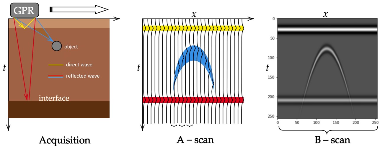
Figure 2: GPR Principle with acquisition (left), creation of the A-scan (middle) and the B-scan (right).

In the next section, we will look at how object type and other parameters influence the shape of the hyperbola.

II-B Influence of the physical parameters on the hyperbola shape

Several factors influence the shape of the hyperbola in the radargram. Firstly, GPR parameters, such as the frequency of the transmitted wave or the elevation of the system relative to the ground, strongly affect the resulting hyperbola. In this article, we will consider several frequencies as well as different GPR elevations. This last point is useful in the case of an airborne GPR, which cannot then be used too close to the ground.

Another factor influencing the shape is obviously the soil and its composition. Each type of soil has its own dielectric permittivity and electrical conductivity, both of which influence the speed of the emitted wave. For example, higher dielectric permittivity generally slows down the propagation of electromagnetic waves or deflects radar waves more than soils with lower permittivity. What’s more, where there are interfaces between different layers, certain variations in these two parameters will be present. These variations will then lead to a deformation of the Ricker wavelet [1].

Finally, the shape of the hyperbola obviously depends on the buried object reflecting the transmitted wave back to the RADAR. Firstly, the size and shape of the object will influence its shape, particularly in the axis of motion of the RADAR. Finally, the electromagnetic properties of the buried object have an impact on the hyperbola, but more in the time axis. Conductive materials, such as metals, absorb more energy and attenuate signals faster than non-conductive materials. To help distinguish between metallic and non-metallic objects, we can look at the polarization of the hyperbola. Polarity reversal occurs when radar waves reflect off objects whose permittivity is higher than that of the surrounding medium (soil has a lower permittivity than metallic objects). To define polarity, we define that the black areas of the hyperbola correspond to a negative polarity ’-’ and the lighter or white areas to a positive polarity ’+’. So, depending on the polarity of the incident wave, a metal object can appear as a positive (+ - +) or negative (- + -) reflection.

We will show some examples of buried object images in the next section.

II-C Examples

On the radargrams in Figure 3, we have used the 200 MHz GSSI antenna which have a positive polarity (+ - +) on wet sand. So a change in polarity will be detected as negative or reversed (- + -). It is therefore more appropriate to speak in terms of normal polarity when the reflection polarity is the same as the incident wave, or reversed polarity when these polarities are different.

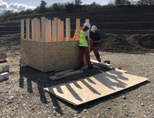
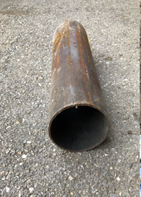
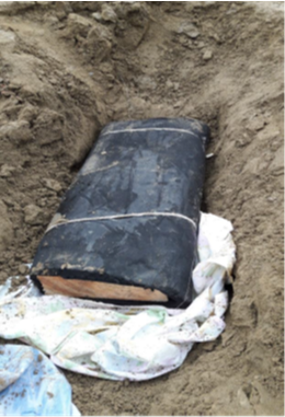
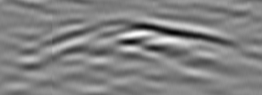
(a)

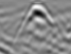
(b)

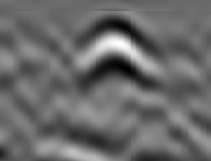
(c)

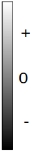
(d)

Figure 3: Examples of preprocessed GPR images with the 200 MHz antenna in wet sand (after direct wave suppression and histogram correction thanks to GPRpy) for different buried objects: Wooden shelter, dummy shell (Metal) and wooden board coated with rubber (Non-Metal). Noticed that the 3 radargrams have different scales.

On the radargram (a), visible in Figure 3, the signature of the shelter consists of:

• A wide hyperbola corresponding to the roof of the shelter (flat surface). The width of the flattened, high-intensity part corresponds to the width of the shelter (2 m). This reflection specifically corresponds to the soil-air interface (rather than soil-wood) due to the significant contrast in dielectric permittivity between air and soil and the thinness of the wood. The polarity is normal ((+ - +) here) same like GSI antenna : there is no change in polarity at the soil-air contact (decrease in dielectric permittivity).

• Two adjacent hyperbolas beneath the first reflection. They correspond to reflections on the corners of the shelter. Their polarity is inverse.

• A wide hyperbola below the previous hyperbolas, corresponding to the base of the shelter.

On the radargram (b).

• Shells are easily recognizable by their high intensity, well-defined hyperbolic shape, and opposite polarity to the GSSI antennas (- + -). The polarity is reversed for metallic object

On the radargram (c)

• wooden board coated with rubber appear in the form of slightly flattened hyperboles is identified by a low intensity hyperbola. Polarity seems reversed (- + -) here.

II-D Goal of the classification model

The 3 previous examples show that the shape of the hyperbola is linked to the buried object. In this article, we therefore propose to build a classification model that takes as input a thumbnail of each hyperbola. We assume that localization and classification have been carried out in the previous steps. Some pre-processing steps are given in [37].

One of the main concerns regarding the classification strategy based on GPR images is robustness. Indeed, we noted in the previous sections that the shape of the hyperbola also depends on parameters other than those of the buried object, such as the GPR and the soil. In this case, the classification must be invariant to these deformations of the hyperbola independently of the object.

The proposed strategy in the next section consists in imposing a transformation on the thumbnail image in order to classify it after this treatment. In particular, we study the interest of the second-order model for achieving good classification performance with good robustness, and all this with relatively little training data.

III Second Order Model

In our task of classifying our radargrams, we rely on neural networks that have shown their effectiveness in image classification tasks.

Let us first describe some of the models that we used as a baseline and illustrate their respective limitations. From this we will then describe our proposed approach that combine several aspects of those models.

Figure 4: Architecture of model CNN1 [42]

III-A Shallow CNN network

As we are considering GPR images thumbnails of pre-localized hyperbolas, the first classes of models that are natural to consider are 2D Convolutional Neural Networks (CNNs) that have been successfully applied in computer vision tasks [43]. Rather than consider large models, and given that we consider very few classes compared to the general image classification problem, shallow CNNs have been considered in [42], where several of such small scale architectures are presented. From this study, we selectioned the best reported model in terms of overall accuracy that is denoted CNN1 whose architecture is reported in Figure 4.

It is constructed as a succession of 3 embedding layers with help of standard 2D convolutions, batch normalization, ReLU non-linearity and max-pooling layers. Then a fully connected layer is followed by a softmax for classes probabilities. While this model allows for classification of the hyperbolas, the obtained accuracies we obtained in practice were not as satisfactory on our dataset, than in the one used in [42], who was trained on synthetic dataset and with a different number of classes. Since our database consists of a great number of real images more difficult to interpret than synthetic ones, it can be intuited that the size of this model is not sufficient for our task.

III-B Computer-vision models

In order to circumvent the lower generalization capabilities of shallow networks, we can consider models that are successful in computer vision tasks. In this work we focused on the ResNet architecture [44]. When using models from the literature, there are two possible approaches:

• Using the pre-trained weights from another task, to benefit from the rich embedding representations and associated classification layers learned on a much bigger dataset. In this case, the weights can be fine-tuned by using the pre-trained values as initialization.

• Given a sufficient enough database size for the task, it is possible to train from scratch. This is useful in situations where the task is very different than traditional computer visions tasks like the GPR classification problem.

In the following, we denote the first model as RFT while the second is RRT.

Such a model is appropriate in handling various classification tasks. However, a problem lies in the very high number of parameters used for the task at hand, making the inference costly compared to the previous shallow model. To address this issue, one can consider taking advantage of recent approaches based upon second-order statistics, which have shown promising results in computer-vision as well as in other applications [39, 40, 41].

III-C SPD models

Covariance representations have been shown to be a relevant description when dealing with noisy signals coming from radar systems [45]. Notably, statistical hypothesis testing over second-order modelling have been successful in target detection in GPR [15]. For classification tasks, building upon [46], a preliminary study over a binary classification problem has been done in [47] using a covariance pooling approach. The idea is to take advantage of the standard convolutional embedding layers that are learned from a computer-vision dataset while employing second-order statistics as a mean to both reduce the dimension of the embedded feature space while also providing additional spatial invariance and better noise handling.

In [48], it is also proposed to further fine-tune the embedding layers by backpropagating the loss gradient over the covariance estimating layers using matrix backpropagation calculus as derived in [49], while introducing more computation than using pre-trained convolutions, is promising for GPR signals that are different than traditional computer vision images.

Figure 5: Illustration of the two architectures used in this paper. In RCNet (Residual Covariance Network), we take only the last output of the ResNet blocks while in SRCNet (Stacked Residual Covariance Network), we stack the first 32 outputs (to save memory space) of the outputs features by interpolating them to a common size of $38\times 20$. With RCNet, we have $h_{L}=54$ and $w_{L}=30$ for the first 3 layers and $h_{L}=28$ and $w_{L}=15$ for the others.

III-D Proposed models

Based on those previous works we propose two architectures names SRCNet and RCNet that take advantage of the covariance pooling approach while adding some layers from the recent model [38] that are specifically designed to handle covariance matrices. The idea behind those layers is to reduce the dimension of the covariance matrices by non-linear dimension reduction while preserving only the information that is relevant for the classification task. The various pipelines used in this paper are illustrated in Figure 5. Let’s describe the different steps of the proposed model:

Resnet34 with $l$ layers: First, we use a non-pretrained ResNet-34 model because the features learned by this model do not seem sufficient to classify our images, especially since we will only use the first $l$ layers that typically contain generally simple features and are effective for covariance matrix calculations. In this paper, we use $l=8$, the layers each yield 64 filters outputs. We start with a grayscale image $\mathbf{I}\in\mathbb{R}^{h\times w}$ whose initial image size $h=112$ and $w=60$ is taken from [50], to provide a basis for comparison in the remainder of this article. We have considered two scenarios (SRCNet and RCNet), in which we retain a portion of the output from each layer or only the last one.

SRCNet: Starting from our grayscale image, the steps are as follows:

• The first $l$ layers of the ResNet34 model each contain $\bar{d}=64$ filters.

• Only $\bar{d}=32$ layers will be retained, in fact we would like to use the information of the first outputs for each layer and capture the main characteristics by calculating the covariance matrix and to save memory space.

• Therefore, the total number of filter outputs is given by $d=l\cdot\bar{d}$.

• Let $\mathbf{I}_{i}\in\mathbb{R}^{h_{i}\times w_{i}}$ with $i\in[1,d]$ represent the set of filter outputs.

• Define $M_{h}$ as the mean of $h_{i}$ and $M_{w}$ as the mean of $w_{i}$.

• We need to resize the filter outputs $\mathbf{I}_{i}$ before stacking. For this purpose, we resize $\mathbf{I}_{i}$ to $\mathbf{\tilde{I}}_{i}\in\mathbb{R}^{M_{h}\times M_{w}}$.

• We then stack the resized filter outputs $\mathbf{\tilde{I}}_{i}$ into a tensor $\mathcal{T}$. Thus, $\mathcal{T}=\{\mathbf{\tilde{I}}_{i}\}_{i\in[1,d]}\in\mathbb{R}^{d\times M_{h}\times M_{w}}$.

• Finally, we reshape $\mathcal{T}$ into $\mathbf{T}$ where $\mathbf{T}\in\mathbb{R}^{d\times M}$ with $M=M_{h}\times M_{w}$.

RCNet: On the other hand, the covariance calculation will be done without stacking the output filters but by taking the layers sequentially with all output filters not just 32. Thus, it will be from the features of the last layer that we will calculate the covariance matrix, d is the total number of output filters from this last layers $l$, in this case $d=64$ for ResNet-34, and $\mathcal{T}=\{\mathbf{\tilde{I}}_{i}\}_{i\in[1,d]}\in\mathbb{R}^{d\times h_{l}\times w_{l}}$ , here we reshape $\mathcal{T}$ into $\mathbf{T}$ where $\mathbf{T}\in\mathbb{R}^{d\times M}$ with $M=h_{l}\times w_{l}$. This adaptation aims to explore the potential benefits of residual connections and optimize the performance of ResNet-34 for our specific GPR data analysis.

Covariance Pooling (CovPool) Layer: Then a covariance pooling layer is added, in fact traditional computer vision models often focus on first-order features, but the significance of second-order relationships in complex scenarios has been widely underestimated. Covariance pooling addresses this gap by incorporating operations on covariance matrices, to capture richer and more complex information about spatial relationships among features and to reduce the dimensionality of the learned features and while preserving correlation information. From $\mathbf{T}$ of SRCNet or RCNet we calculate:

$$\mathbf{C}=\mathbf{T}\bar{\mathbf{I}}\mathbf{T}^{\mathrm{T}},$$

where $\bar{\mathbf{I}}=\frac{1}{N}\left(\mathbf{I}-\mathbf{1}_{N}\mathbf{1}_{N}^{\mathrm{T}}\right)$ and $\mathbf{C}\in\ \mathbb{R}^{d\times d}$ is a SPD Matrix (denoted SPD for Symmetric Positive Definite).

SPD Net Layer [38]: The obtained covariance matrix $\mathbf{C}$ can then be of very high dimension, and it seems interesting to reduce the data space for better performance. Therefore, we suggest adding convolutional layers adapted to covariance matrices using the framework proposed in [38], denoted as SPD Net. SPD Net is a model that, for $k\geq 1$, takes as input a matrix $\bm{X}_{k-1}\in\text{Sym}_{d_{k-1}}^{+}$. In our case, we start with $\mathbf{X}_{0}=\mathbf{C}\in\ \mathbb{R}^{d\times d}$, a symmetric positive definite matrix of size $d_{k-1}$. The dimensionality of the space is reduced through several BiMap convolution layers and a ReEig regularization layer based on an Eigenvalue Decomposition (EVD). These two steps can be repeated multiple times. Finally, there is a LogEig layer to perform measurements between covariance matrices in a common space (tangent plane to the Riemannian manifold of SPD matrices taken at the identity). The unknowns in the problem are the convolution matrices $\bm{W}_{k}\in\mathbb{R}_{*}^{d_{k}\times d_{k-1}}$, which are low-rank and belong to a Stiefel manifold.

Here are some details about the different layers at each step of the forward propagation:

• BiMap Layer (to generate more compact and discriminative SPD matrices):

  $$\mathbf{X}_{k}=f_{b}^{(k)}(\mathbf{X}_{k-1};\mathbf{W}_{k})=\mathbf{W}_{k}\mathbf{X}_{k-1}\mathbf{W}_{k}^{T},$$

  where $\bm{X}_{k-1}$ is the input SPD matrix of the $k$-th layer, $\bm{W}_{k}\in\mathbb{R}_{*}^{d_{k}\times d_{k-1}},(d_{k}<d_{k-1})$ is the orthonormal transformation matrix (connection weights), $\bm{X}_{k}\in\mathbb{R}^{d_{k}\times d_{k}}$ is the resulting matrix and $f_{b}^{(k)}$ is the function for the $k$-th layer.

• ReEig Layer (to improve discriminative performance, inspired by ReLU):

  $$\mathbf{X}_{k}=f_{r}^{(k)}(\mathbf{X}_{k-1})=\mathbf{U}_{k-1}\max(\epsilon\mathbf{I},\bm{\Sigma}_{k-1})\mathbf{U}_{k-1}^{T},$$

  where eigenvalue decomposition (EIG) of $\bm{X}_{k-1}=\mathbf{U}_{k-1}\bm{\Sigma}_{k-1}\mathbf{U}_{k-1}^{T},\epsilon$ is a rectification threshold, $\mathbf{I}$ is an identity matrix and $\max\left(\epsilon\mathbf{I},\bm{\Sigma}_{k-1}\right)$ is a diagonal matrix of the corrected eigenvalues in order to stay on the SPD manifold.

These both steps, BiMap and ReEig layers, could be repeated several times in order to find the best representation for the classification.

Figure 6: Matrix backpropagation principle. Solid lines correspond to forward pass and dashed lines to backward pass. $\bm{\theta}$ are the learned parameters: $\bm{\theta}_{l}=\mathbf{W}_{l}$ for BiMap layers while $\bm{\theta}=\emptyset$ otherwhise. $\mathbf{X}$ is the tensor after ResNet layers and $\hat{y}$ is the classification output.

In the final stage of the model, we aim to classify a lower-dimensional discriminant SPD (Symmetric Positive Definite) matrix. To enable the application of traditional fully connected (FC) layers, we first transform the SPD matrix into a feature in Euclidean space. This transformation is performed using the LogEig operator, which calculates the matrix logarithm of the input:

$$\mathbf{X}_{k}=f_{l}^{(k)}(\mathbf{X}_{k-1})=\mathbf{U}_{k-1}\log(\bm{\Sigma}_{k-1})\mathbf{U}_{k-1}^{T},$$

where $\log(\bm{\Sigma}_{k-1})$ is the diagonal matrix of logarithms of the eigenvalues of the SPD matrix, from the EVD of $\mathbf{X}_{k-1}$ as with ReEig layer. Finally, we vectorize the resulting matrix before the FC layers and we introduce a dropout mechanism to mitigate the risk of overfitting.

Back-propagation Steps: Since the main steps are matrix operations, the backward is not classical like in most of deep learning models. In particular, the gradients of the operations based on SVD have been firstly derived in [51]. A more stable formula is given in [40] and will be used. An illustration of the backpropagation steps can be found in Figure 6. Calculations concerning $\mathbf{W}_{k}$ differ, as they are based on Riemannian gradient descent on the Stiefel manifold, where $\mathbf{W}_{k}$ represents an orthonormal matrix. Detailed explanations of this approach can be found in [38]. Let us summarize hereafter the steps of the backpropagation for the proposed model.

Given loss function $\mathcal{L}:\mathbb{R}^{K},\mathbb{R}^{K}\rightarrow\mathbb{R}$, where $K$ is the number of classes. By denoting $f_{l}$ the $l$-th layer in the network, we can define the loss starting at this layer as

$$\mathcal{L}^{l}=\underbrace{\mathcal{L}\circ f_{\ell}\circ\dots f_{l-1}}_{\mathcal{L}^{l-1}}\circ f_{l},$$

where $\ell$ is the number of total layers in the network.

Given those definitions, the backpropagation steps are as follows:

• CovPool Layer: Let us consider this layer as some $f_{l}$ in the network, meaning $\mathbf{C}=f_{l}(\mathbf{T})=\mathbf{T}\bar{\mathbf{I}}\mathbf{T}^{T}$ and suppose that we have already calculated $\frac{\partial\mathcal{L}^{l+1}}{\partial\mathbf{C}}$. Since there is no parameter to learn, the matrix chain-rule [51] on $\mathcal{L}^{l}(\mathbf{T})=\mathcal{L}^{l+1}\circ f_{l}(\mathbf{T})$ yields:

  $$\langle\frac{\partial\mathcal{L}^{l+1}}{\partial\mathbf{C}},\mathrm{d}\mathbf{C}\rangle=\langle\frac{\partial\mathcal{L}^{l}}{\partial\mathbf{T}},\mathrm{d}\mathbf{T}\rangle,$$

  where $\langle\cdot,\cdot\rangle$ is the Frobenius inner product. We have that $\mathrm{d}\mathbf{C}=(\mathrm{d}\mathbf{T})\bar{\mathbf{I}}\mathbf{T}^{\mathrm{T}}+\mathbf{T}\bar{\mathbf{I}}(\mathrm{d}\mathbf{T})^{\mathrm{T}}$ and using symmetries on $\bar{\mathbf{I}}$ yields:

  $$\frac{\partial\mathcal{L}^{l}}{\partial\mathbf{T}}=2\bar{\mathbf{I}}\mathbf{T}^{\mathrm{T}}\frac{\partial\mathcal{L}^{l+1}}{\partial\mathbf{C}}.$$

• BiMap Layer: for this layer, we have two gradients to propagate : $\frac{\partial\mathcal{L}^{l}}{\partial\mathbf{X}_{l-1}}$, the gradient towards the input of the layer and $\frac{\partial\mathcal{L^{l}}}{\partial\mathbf{W}}$, the gradient to update the weights $\mathbf{W}$ of the bilinear mapping to be learned. We can make use of the same matrix backpropagation principle with $f_{l}:\mathcal{S}^{d_{l-1}}\times\mathcal{O}_{d_{l}\times d_{l-1}}\rightarrow\mathcal{S}^{d_{l}}$, where $\mathcal{O}_{m\times n}$ is the set of orthonormal matrices of size $m\times n$, and $f_{l}(\mathbf{X}_{l})=\mathbf{W}\mathbf{X}_{l-1}\mathbf{W}^{T}$, the gradients are given by :

  $$\begin{array}[]{lll}\frac{\partial\mathcal{L}^{l}}{\partial\mathbf{X}_{l-1}}&=&\mathbf{W}^{\mathrm{T}}\frac{\partial\mathcal{L}^{l+1}}{\partial\mathbf{X}_{l}}\mathbf{W}\\ \frac{\partial\mathcal{L}^{l}}{\partial\mathbf{W}}&=&2\frac{\partial\mathcal{L}^{l+1}}{\partial\mathbf{X}_{l}}\mathbf{W}\mathbf{X}_{l-1}\end{array}.$$

  One additional thing to take into account is that $\mathbf{W}$ has a special structure. Thus, while doing the gradient step, it is necessary to use a Riemannian retraction operator [52] to keep the weights on the Stiefel manifold.

• ReEig and LogEig Layer: Since both operations operate on eigenvalue decomposition, we can decompose $f_{l}$ as $f_{l}=f_{l}^{{}^{\prime}}\circ\mathrm{eig}$ where $\mathrm{eig}$ means doing the EVD of the input matrix an$f_{l}^{{}^{\prime}}$ is the operation on the eigenvalues and reconstructing the matrix. The gradient towards input is given by [40]:

  $$\frac{\partial\mathcal{L}^{l}}{\partial\mathbf{X}_{l-1}}= 2\mathbf{U}_{l-1}\left(\mathbf{P}^{\mathrm{T}}\odot\left(\mathbf{U}_{l-1}^{\mathrm{T}}\frac{\partial\mathcal{L}^{l+1}\circ f_{l}^{{}^{\prime}}}{\partial\mathbf{U}_{l-1}}\right)_{sym}\right)\mathbf{U}_{l-1}^{\mathrm{T}}$$

  $$+\mathbf{U}_{l-1}\left(\frac{\partial\mathcal{L}^{l+1}\circ f_{l}^{{}^{\prime}}}{\partial\bm{\Sigma}_{l-1}}\right)_{diag}\mathbf{U}_{l-1}^{\mathrm{T}},$$

  where $\mathbf{P}$ is a square matrix given by

  $$\mathbf{P}(i,j)=\begin{cases}\frac{1}{\sigma_{i}-\sigma_{j}}&\text{if }i\neq j,\\ 0&\text{otherwise}\end{cases},$$

  and $\sigma_{i}$ are the eigenvalues of $\mathbf{X}_{l-1}$.

  For the ReEig layer, the sub-gradients are given by:

  $$\frac{\partial\mathcal{L}^{l+1}\circ f_{l}^{{}^{\prime}}}{\partial\mathbf{U}_{l-1}} =2\left(\frac{\partial\mathcal{L}^{l+1}}{\partial\mathbf{X}_{l}}\right)_{sym}\mathbf{U}_{l-1}\mathrm{max}(\epsilon\mathbf{I},\bm{\Sigma}_{l-1}),$$

  $$\frac{\partial\mathcal{L}^{l+1}\circ f_{l}^{{}^{\prime}}}{\partial\bm{\Sigma}_{l-1}} =\mathbf{Q}\mathbf{U}_{l-1}^{\mathrm{T}}\left(\frac{\partial\mathcal{L}^{l+1}}{\partial\mathbf{X}_{l}}\right)_{sym}\mathbf{U}_{l-1},$$

  where $\mathbf{Q}$ is a diagonal matrix with elements:

  $$\mathbf{Q}(i,i)=\begin{cases}1&\text{if }\bm{\Sigma}_{l-1}(i,i)>\epsilon,\\ 0&\text{otherwise}.\end{cases}$$

  For the LogEig layer, the sub-gradients are given by:

  $$\frac{\partial\mathcal{L}^{l+1}\circ f_{l}^{{}^{\prime}}}{\partial\mathbf{U}_{l-1}} =2\left(\frac{\partial\mathcal{L}^{l+1}}{\partial\mathbf{X}_{l}}\right)_{sym}\mathbf{U}_{l-1}\log(\bm{\Sigma}_{l-1}),$$

  $$\frac{\partial\mathcal{L}^{l+1}\circ f_{l}^{{}^{\prime}}}{\partial\bm{\Sigma}_{l-1}} =\bm{\Sigma}_{l-1}^{-1}\mathbf{U}_{l-1}^{\mathrm{T}}\left(\frac{\partial\mathcal{L}^{l+1}}{\partial\mathbf{X}_{l}}\right)_{sym}\mathbf{U}_{l-1}.$$

Thanks to all these steps, there is a backpropagation for all the layers from the final fully-connected layers to the ResNet34 convolution layers. This means that contrarily to previous works [34, 38] we make advantage of both the bilinear mapping with learnable weights to obtain a discriminative SPD matrix for classification but also the best convolutions and thus embedding space for the task at hand rather than keeping pre-trained weights on another task.

Implementation: we provide a pyTorch implementation of those steps available at https://github.com/ammarmian/anotherspdnet.

Let us now present the experimental results obtained with the proposed models in the next sections.

IV Dataset description

The database provided by the Geolithe company include 699 medium-sized radargrams of $(R_{x},R_{y})=(4000,800)$ pixels, along with all the necessary acquisition information such as radar frequency (200MHz or 350MHz for Geolithe), radar elevation (0cm, 25cm, 50cm, 75cm, 100cm, 150cm), and soil type (wet sand, dry sand, gravel, dry gravel). Each radargram is associated with a mask of the same size. Main preprocessing steps [37] consists to determine the rectangle around each hyperbola in the radargram by using the mask image in order to build a thumbnail image for each target. An example of this preprocessing for one radargram is shown in 7. All thumbnails are resized to $(w,h)=(60,112)$ before to be treated by the different classification methods. We have also created a class denoted ”empty” (in yellow in the figure 7) which is randomly placed on the radargram.

Figure 7: Example for one radargram (bottom) and the corresponding image of the masks. The positions of the rectangles detected on the masks were projected onto the radargrams. The yellow rectangles correspond to a thumbnail of the empty class.

The final database then consists of 1584 thumbnails, classified into four categories: Metallic, Non-Metallic, Wooden Shelters, and Empty. Tables I and II provides more details on the distribution of the four categories according to elevation, soil and frequency. As used classicaly in supervized approaches, we divide our dataset into three distinct parts: a training set consisting of 1108 images, a validation set with 238 images, and finally, a test set also comprising 238 images. The latter will be used to evaluate the accuracy of the different tested models.

	Wooden Shelter				Metallic				Non Metallic				Empty				Total
Soil/Elevation (cm)	25	50	75	100	25	50	75	100	25	50	75	100	25	50	75	100
grave	20	16	12	4	13	17	6	11	16	14	8	4	20	12	18	12	203
dry grave	24	18	17	19	18	14	16	6	14	15	14	10	15	19	19	20	258
sand	37	44	48	54	48	40	55	50	40	44	44	48	45	50	45	43	735
wet sand	18	21	22	22	20	28	22	32	29	26	33	37	19	18	17	24	388
Total	99	99	99	99	99	99	99	99	99	99	99	99	99	99	99	99	1584

TABLE I: Distribution of our database for each soil and depending on the elevation of GPR.

	Wooden Shelter				Metallic				Non Metallic				Empty				Total
Frequency/Elevation (cm)	25	50	75	100	25	50	75	100	25	50	75	100	25	50	75	100
200 MHZ	53	46	54	49	24	13	19	18	26	28	26	20	40	46	45	40	547
350 MHZ	46	53	45	50	75	86	80	81	73	71	73	79	59	53	54	59	1037
Total	99	99	99	99	99	99	99	99	99	99	99	99	99	99	99	99	1584

TABLE II: Distribution of our database for each frequency and depending on the elevation of GPR.

V Numerical experiments

V-A List of models

As described in section III, we consider in this paper three models with small variation which are recalled in the following:

• CNN1: the shallow architecture developed in [50] for GPR image classification

• Resnet34: a deep network proposed in [44] initially applied to computer vision applications. In this section we will consider two models from this architecture:

  • RRT: the model is then trained from scratch, which we initialize the weights randomly.

  • RFT: the model is fine-tuned which consists in trained by using the pre-trained weights. In this specific model, they are pre-trained from the ImageNet database.

• Our proposed models in two configurations:

  • SRCNet: all the $l$ first layers (only 32 output filters are selected for each layers to save memory space) are considered to build our tensor. In this case the first size of the SPD matrix is $d_{0}=256$.

  • RCNet: only the last layer with these 64 output filters are used to build the tensor. In this case the first size of the SPD matrix is $d_{0}=64$.

  For these both models, the number of layers of Resnet34 to build the tensor $\mathcal{T}$ is $l=8$. Moreover, SPD Net is designed with 4 consecutive BiMap and ReEig layers where the sizes of each SPD matrices are specified in Table III. The choice of 4 layers is common when using SPD Net [38] and in particular it is shown in different experiments [53] that it is useless to take more than 4 consecutive BiMap and ReEig layers.

All models are used with the same parameters each time. The chosen optimizer is SGD with a momentum of 0.9, a batch size of 8, and a learning rate of 0.007.

	$d_{0}$	$d_{2}$	$d_{4}$	$d_{6}$	$d_{8}$
SRCNet	256	235	217	179	128
RCNet	64	58	54	44	32

TABLE III: Output dimensions of SPDNet layers (BiMap and ReEig).

In the following subsections, we compare all these models with our database described in IV, first by measuring the influence of the number of training data on the classification results, then the robustness in the presence of mislabeled data in the training set, and finally the robustness to data shifts between the training set and the test set. In all experiments, 100 different random generator seeds are used to construct the partition between training and testing data sets. This allows to obtain more representative results irrespective of the initilialization. To showcase results, we decide to show the 5-th, 50-th and 95-th quantiles of the performance metric.

V-B Influence of the number of training data

First, we study the influence of the number of training data. Indeed, it is really difficult to collect a large labelled data base for GPR applications since it is very time consuming and that geophysics experts are absolutely needed. Therefore, it is important to design classification models which can provide good performance with a limited training dataset. The results of test accuracy w.r.t training ratio are shown in Figure 8. We can observe that our proposed approaches, SRCNet and RCNet both outperform the classical approaches at any given training ratio and have lower variability over seeds. The Resnet34 approaches perform better than [30] especially when the number of training data increases. The retraining approach, RRT, gives better results compared to the fine-tuning approach, RFT, in particular when the training ratio becomes smaller.

Figure 8: Results of test accuracy w.r.t to training dataset percentage over 100 different seeds. For each method, the line corresponds to the mean of accuracy over all the seeds, and the filled area corresponds to 5-th and 95-th quantiles.

V-C Robustness to mislabeled Data

The second simulation studies the effect to have mislabeled data in the training data set. Actually it can be difficult to correctly labeled the hyperbola in particular because of the low Signal to Noise Ratio (SNR) in radargram. For this simulation, we introduce a variable level of mislabeled data, 0 to 20% of error, in the training set. The results of test accuracy w.r.t mislabelling percentage are presented in Figure 9. We have comparable dynamic than the previous experiment with better performance and robustness of RCNet and SRCNet (with a better result when considering only the last layer for the tensor construction). The case of [30] is interesting as it shows that shallow models performance decreases quickly as soon as there are a few mislabelled data. as before, we observe that our approaches have the least variability over the seeds. In conclusion, this result is in line with the analysis made in [54], which also shows that covariance matrix utilization brings great robustness to mislabeled data in metric learning methods.

Figure 9: Results of test accuracy w.r.t training dataset mislabelling percentage. For each method, the line corresponds to the mean of accuracy over all the seeds, and the filled area corresponds to 5-th and 95-th quantiles. The legends are the same as in Fig. 8.

V-D Robustness to data shift

In many applications, it is common for data to undergo various transformations between the training set and the test set, which can be scaling, translation, covariate shifts, … [55]. In addition, for some specific applications like GPR, where labeling is quite difficult, it may be impossible to train our model taking into account all RADAR features, all soils and even all meteorological considerations. This is why we consider it important to propose classification algorithms that are robust to these possible changes between training and test data. To study the behavior of the models proposed in this paper, we consider 4 scenarios:

• Scenario A: the training and validation sets include images obtained using a RADAR located at an altitude of 75 cm or 100 cm, while the test set is made up of images acquired at an altitude of 50 cm.

• Scenario B: the frequency is chosen at 200 MHz for the training and validation sets, while the test set uses only data obtained with a frequency of 350 MHz.

• Scenario C: the training and validation sets are made up of data acquired in dry gravel, whereas the test set uses gravel.

• Scenario D: same scenario as C, with wet sand for the training and validation sets, and dry sand for the test set.

The distribution and number of elements in the sets for each scenario are detailed in table IV.

	Train	Val	Test
A: ELV 75,100 vs 50	634	79	79
B: FRQ 350 vs 200	394	49	49
C: GRD Dry Gravel vs Gravel	394	49	49
D: GRD Wet Sand vs Dry Sand	672	84	84

TABLE IV: Distribution of the training, validation and test sets for the 4 scenario.

V-D1 Scenario A

In Figure 10 we represent five boxplots given the accuracy performances of the different models. We easily concluded that our models, in particular RCNet performance is almost unchanged compared to the classical case, are particular robust to this transformation. In this case, main transformations are scaling but the shape of the hyperbola slightly changes. As expected, the shallow model is the less robust. We also noticed that the variability over the seeds is very small with the models built from covariance matrix. This result is also in line with those obtained in [36] where covariance matrix are used to classify crops in Satellite Image Times Series.

Figure 10: Results of test accuracy results for scenario A.

V-D2 Scenario B

The box diagrams are now shown in figure 11. As in the previous scenario, the models we propose outperform the surface and computer vision models. But in this case, the best algorithm is SRCNet and we notice a sharp degradation in the performance of all approaches. The number of transformations between the two sets is then too high. This is because the frequency is linked to the penetration of the wave into the ground, as well as to the possible resolution which results in very different radargrams.

Figure 11: Results of test accuracy results for scenario B.

V-D3 Scenario C and D

The boxplots for the scenario C are shown in 12 while those for the scenario D are given in 13. In both cases, the second order deep learning models give better results and lower variabilities. We can conclude that if we want to obtain robust performances, it is clear that our approaches are better suited than shallow models or classical deep learning models as Resnet34.

Figure 12: Results of test accuracy results for scenario C.

Figure 13: Results of test accuracy results for scenario D.

VI Conclusion

In this paper, we have proposed a new deep learning model based on second-order moments to classify buried objects from the hyperbola thumbnails obtained with a classical GPR system. The proposed model is the concatenation of several models: the first is composed of the first layers of a classical CNN and is used to obtain a covariance matrix from the outputs of convolutional filters, while the second is composed of specific layers to classify SPD matrices. These models are tested on a database composed of several radargrams and compared with shallow models and conventional CNNs typically used in computer vision applications. Our approach gives better results, particularly when the number of training data decreases and in the presence of mislabeled data. We also illustrated the value of second-order deep learning models when training data and test sets are obtained from different weather modes or considerations.

References

- [1] David J Daniels, Ground Penetrating Radar, IEE, 2004.
- [2] Harry M. Jol, Ed., Ground Penetrating Radar: Theory and Applications, Elsevier, 2009.
- [3] Andrea Benedetto, Fabio Tosti, Luca Bianchini Ciampoli, and Fabrizio D’Amico, “An overview of ground-penetrating radar signal processing techniques for road inspections,” Signal Processing, vol. 132, pp. 201–209, 2017.
- [4] A.C. Gurbuz, J.H. McClellan, and W.R. Scott, “A compressive sensing data acquisition and imaging method for stepped frequency GPRs,” Signal Processing, IEEE Transactions on, vol. 57, no. 7, pp. 2640–2650, July 2009.
- [5] Zhaofa Zeng, Jing Li, Ling Huang, Xuan Feng, and Fengshan Liu, “Improving target detection accuracy based on multipolarization MIMO GPR,” Geoscience and Remote Sensing, IEEE Transactions on, vol. 53, no. 1, pp. 15–24, Jan 2015.
- [6] Bin Liu, Yuxiao Ren, Hanchi Liu, Hui Xu, Zhengfang Wang, Anthony G. Cohn, and Peng Jiang, “GPRInvNet: Deep learning-based ground-penetrating radar data inversion for tunnel linings,” IEEE Transactions on Geoscience and Remote Sensing, vol. 59, no. 10, pp. 8305–8325, 2021.
- [7] Xingkun He, Can Wang, Rongyao Zheng, Zhibin Sun, and Xiwen Li, “Gpr image denoising with NSST-UNET and an improved BM3D,” Digital Signal Processing, vol. 123, pp. 103402, 2022.
- [8] Qiqi Dai, Yee Hui Lee, Hai-Han Sun, Genevieve Ow, Mohamed Lokman Mohd Yusof, and Abdulkadir C. Yucel, “Dmrf-unet: A two-stage deep learning scheme for gpr data inversion under heterogeneous soil conditions,” IEEE Transactions on Antennas and Propagation, pp. 1–1, 2022.
- [9] Zhi-Kang Ni, Jun Pan, Cheng Shi, Shengbo Ye, Di Zhao, and Guangyou Fang, “DL-Based Clutter Removal in Migrated GPR Data for Detection of Buried Target,” vol. 19, pp. 1–5, 2022, Conference Name: IEEE Geoscience and Remote Sensing Letters.
- [10] Paolo Bestagini, Federico Lombardi, Maurizio Lualdi, Francesco Picetti, and Stefano Tubaro, “Landmine detection using autoencoders on multipolarization gpr volumetric data,” IEEE Transactions on Geoscience and Remote Sensing, vol. 59, no. 1, pp. 182–195, 2021.
- [11] Christian Maas and Jörg Schmalzl, “Using pattern recognition to automatically localize reflection hyperbolas in data from ground penetrating radar,” Computers and Geosciences, vol. 58, pp. 116–125, 2013.
- [12] H. Brunzell, “Detection of shallowly buried objects using impulse radar,” IEEE Transactions on Geoscience and Remote Sensing, vol. 37, no. 2, pp. 875–886, 1999.
- [13] A.M. Zoubir, I.J. Chant, C.L. Brown, B. Barkat, and C. Abeynayake, “Signal processing techniques for landmine detection using impulse ground penetrating radar,” Sensors Journal, IEEE, vol. 2, no. 1, pp. 41–51, Feb 2002.
- [14] K.C. Ho and P.D. Gader, “A linear prediction land mine detection algorithm for hand held ground penetrating radar,” IEEE Transactions on Geoscience and Remote Sensing, vol. 40, no. 6, pp. 1374–1384, 2002.
- [15] Q. Hoarau, G. Ginolhac, A. M. Atto, and J. M. Nicolas, “Robust adaptive detection of buried pipes using GPR,” Signal Processing, vol. 132, pp. 293–305, Mar. 2017.
- [16] W. Ng, T. Chan, H.C. So, and K.C. Ho, “Particle filtering based approach for landmine detection using Ground Penetrating Radar,” Geoscience and Remote Sensing, IEEE Transactions on, vol. 46, no. 11, pp. 3739–3755, Nov 2008.
- [17] A. Manandhar, P.A. Torrione, L.M. Collins, and K.D. Morton, “Multiple-instance hidden markov model for gpr-based landmine detection,” Geoscience and Remote Sensing, IEEE Transactions on, vol. 53, no. 4, pp. 1737–1745, April 2015.
- [18] V. Kovalenko, A.G. Yarovoy, and L.P. Ligthart, “A novel clutter suppression algorithm for landmine detection with GPR,” Geoscience and Remote Sensing, IEEE Transactions on, vol. 45, no. 11, pp. 3740–3751, Oct 2007.
- [19] Jing Li, Cai Liu, Zhaofa Zeng, and Lingna Chen, “Gpr signal denoising and target extraction with the ceemd method,” IEEE Geoscience and Remote Sensing Letters, vol. 12, no. 8, pp. 1615–1619, 2015.
- [20] Jianping Wang, Pascal Aubry, and Alexander Yarovoy, “Efficient implementation of gpr data inversion in case of spatially varying antenna polarizations,” IEEE Transactions on Geoscience and Remote Sensing, vol. 56, no. 4, pp. 2387–2396, 2018.
- [21] Guillaume Terrasse, Jean-Marie Nicolas, Emmanuel Trouvé, and Émeline Drouet, “Sparse decomposition of the GPR useful signal from hyperbola dictionary,” in 2016 24th European Signal Processing Conference (EUSIPCO), 2016, pp. 2400–2404.
- [22] Michele Ambrosanio and Vito Pascazio, “A compressive-sensing-based approach for the detection and characterization of buried objects,” IEEE Journal of Selected Topics in Applied Earth Observations and Remote Sensing, vol. 8, no. 7, pp. 3386–3395, 2015.
- [23] Fabio Giovanneschi, Kumar Vijay Mishra, Maria Antonia Gonzalez-Huici, Yonina C. Eldar, and Joachim H. G. Ender, “Dictionary learning for adaptive gpr landmine classification,” IEEE Transactions on Geoscience and Remote Sensing, vol. 57, no. 12, pp. 10036–10055, 2019.
- [24] Matthieu Gallet, Ammar Mian, Guillaume Ginolhac, Esa Ollila, and Nickolas Stelzenmuller, “New robust sparse convolutional coding inversion algorithm for ground penetrating radar images,” IEEE Transactions on Geoscience and Remote Sensing, 2023.
- [25] Wenbin Shao, Abdesselam Bouzerdoum, and Son Lam Phung, “Sparse representation of gpr traces with application to signal classification,” IEEE Transactions on Geoscience and Remote Sensing, vol. 51, no. 7, pp. 3922–3930, 2013.
- [26] Fok Hing Chi Tivive, Abdesselam Bouzerdoum, and Canicious Abeynayake, “Gpr signal classification with low-rank and convolutional sparse coding representation,” in 2017 IEEE Radar Conference (RadarConf), 2017, pp. 1352–1356.
- [27] W. Shao, A. Bouzerdoum, S. L. Phung, L. Su, B. Indraratna, and C. Rujikiatkamjorn, “Automatic classification of GPR signals,” in Proceedings of the XIII Internarional Conference on Ground Penetrating Radar, June 2010, pp. 1–6.
- [28] Haoqiu Zhou, Xuan Feng, Yan Zhang, Enhedelihai Nilot, Minghe Zhang, Zejun Dong, and Jiahui Qi, “Combination of Support Vector Machine and H-Alpha Decomposition for Subsurface Target Classification of GPR,” in 2018 17th International Conference on Ground Penetrating Radar (GPR), June 2018, pp. 1–4, ISSN: 2474-3844.
- [29] Lance E. Besaw and Philip J. Stimac, “Deep convolutional neural networks for classifying GPR B-scans,” in Detection and Sensing of Mines, Explosive Objects, and Obscured Targets XX. May 2015, vol. 9454, pp. 385–394, SPIE.
- [30] Maha Almaimani, Dalei Wu, Yu Liang, Li Yang, Dryver Huston, and Tian Xia, Classifying GPR Images Using Convolutional Neural Networks, Jan. 2018.
- [31] Xisto L. Travassos, Sérgio L. Avila, and Nathan Ida, “Artificial Neural Networks and Machine Learning techniques applied to Ground Penetrating Radar: A review,” Applied Computing and Informatics, vol. 17, no. 2, pp. 296–308, Jan. 2020, Publisher: Emerald Publishing Limited.
- [32] Mostafa Elsaadouny, Jan Barowski, and Ilona Rolfes, “ConvNet Transfer Learning for GPR Images Classification,” in 2020 German Microwave Conference (GeMiC), Mar. 2020, pp. 21–24, ISSN: 2167-8022.
- [33] Sara Akodad, Lionel Bombrun, Junshi Xia, Yannick Berthoumieu, and Christian Germain, “Ensemble learning approaches based on covariance pooling of CNN features for high resolution remote sensing scene classification,” Remote Sensing, vol. 12, no. 20, pp. 3292, 2020.
- [34] Peihua Li, Jiangtao Xie, Qilong Wang, and Wangmeng Zuo, “Is second-order information helpful for large-scale visual recognition?,” in Proceedings of the IEEE ICCV, 2017, pp. 2070–2078.
- [35] Peihua Li, Jiangtao Xie, Qilong Wang, and Zilin Gao, “Towards faster training of global covariance pooling networks by iterative matrix square root normalization,” in Proceedings of the IEEE CVPR, 2018, pp. 947–955.
- [36] Antoine Collas, Arnaud Breloy, Chengfang Ren, Guillaume Ginolhac, and Jean-Philippe Ovarlez, “Riemannian optimization for non-centered mixture of scaled gaussian distributions,” IEEE Transactions on Signal Processing, vol. 71, pp. 2475–2490, 2023.
- [37] Matthieu Gallet, Ammar Mian, Guillaume Ginolhac, and Nickolas Stelzenmuller, “Classification of GPR signals via covariance pooling on CNN features within a riemannian framework,” in IGARSS 2022. IEEE, 2022, pp. 365–368.
- [38] Zhiwu Huang and Luc Van Gool, “A riemannian network for SPD matrix learning,” in Proceedings of the AAAI conference on artificial intelligence, 2017, vol. 31.
- [39] Reinmar Kobler, Jun-ichiro Hirayama, Qibin Zhao, and Motoaki Kawanabe, “Spd domain-specific batch normalization to crack interpretable unsupervised domain adaptation in eeg,” in Neurips 2022, 2022.
- [40] Daniel Brooks, Olivier Schwander, Frédéric Barbaresco, Jean-Yves Schneider, and Matthieu Cord, “Riemannian batch normalization for SPD neural networks,” Advances in Neural Information Processing Systems, vol. 32, 2019.
- [41] Junfei Shi, Wei Wang, Haiyan Jin, Mengmeng Nie, and Shanshan Ji, “Riemannian complex matrix convolution network for polsar image classification,” 2023.
- [42] Maha Almaimani, Dalei Wu, Yu Liang, Li Yang, Dryver Huston, and Tian Xia, Classifying GPR Images Using Convolutional Neural Networks, Jan. 2018.
- [43] Alex Krizhevsky, Ilya Sutskever, and Geoffrey E Hinton, “Imagenet classification with deep convolutional neural networks,” Advances in neural information processing systems, vol. 25, 2012.
- [44] Kaiming He, Xiangyu Zhang, Shaoqing Ren, and Jian Sun, “Deep residual learning for image recognition,” in Proceedings of the IEEE conference on computer vision and pattern recognition, 2016, pp. 770–778.
- [45] E. Ollila, D. E. Tyler, V. Koivunen, and H. V. Poor, “Complex elliptically symmetric distributions: Survey, new results and applications,” IEEE Transactions on Signal Processing, vol. 60, no. 11, pp. 5597–5625, 2012.
- [46] Sara Akodad, Lionel Bombrun, Maria Puscasu, Junshi Xia, Christian Germain, and Yannick Berthoumieu, “Deep Ensemble Learning Model Based on Covariance Pooling of Multi-Layer CNN Features,” in 2022 IEEE International Conference on Image Processing (ICIP), Bordeaux, France, Oct. 2022, pp. 1081–1085, IEEE.
- [47] Matthieu Gallet, Ammar Mian, Guillaume Ginolhac, and Nickolas Stelzenmuller, “Classification of GPR signals via covariance pooling on CNN features within a riemannian framework,” in IGARSS 2022 - 2022 IEEE International Geoscience and Remote Sensing Symposium, 2022, pp. 365–368.
- [48] Peihua Li, Jiangtao Xie, Qilong Wang, and Wangmeng Zuo, “Is second-order information helpful for large-scale visual recognition?,” in Proceedings of the IEEE international conference on computer vision, 2017, pp. 2070–2078.
- [49] Catalin Ionescu, Orestis Vantzos, and Cristian Sminchisescu, “Matrix backpropagation for deep networks with structured layers,” in 2015 IEEE International Conference on Computer Vision (ICCV), 2015, pp. 2965–2973.
- [50] Maha Almaimani, “Classifying GPR images using convolutional neural networks,” 2018.
- [51] Catalin Ionescu, Orestis Vantzos, and Cristian Sminchisescu, “Training deep networks with structured layers by matrix backpropagation,” 2015.
- [52] Nicolas Boumal, An introduction to optimization on smooth manifolds, Cambridge University Press, 2023.
- [53] Rui Wang, Xiao-Jun Wu, Ziheng Chen, Tianyang Xu, and Josef Kittler, “DreamNet: A deep Riemannian manifold network for SPD matrix learning,” in Proceedings of the 16th Asian Conference on Computer Vision (ACCV2022), 2022.
- [54] Antoine Collas, Arnaud Breloy, Guillaume Ginolhac, Chengfang Ren, and Jean-Philippe Ovarlez, “Robust geometric metric learning,” in Proceedings of EUSIPCO 2022, Aug. 2022.
- [55] Mingsheng Long, Yue Cao, Jianmin Wang, and Michael Jordan, “Learning transferable features with deep adaptation networks,” in Proceedings of the 32nd International Conference on Machine Learning, Lille, France, 07–09 Jul 2015, vol. 37 of Proceedings of Machine Learning Research, pp. 97–105, PMLR.