Multiple Pareto-optimal solutions of the dissipation-adaptation trade-off

Abstract

Adaptation refers to the ability to recover and maintain “normal” function upon perturbations of internal of external conditions and is essential for sustaining life. Biological adaptation mechanisms are dissipative, i.e. they require a supply of energy such as the coupling to the hydrolysis of ATP. Via evolution the underlying biochemical machinery of living organisms evolved into highly optimized states. However, in the case of adaptation processes two quantities are optimized simultaneously, the adaptation speed or accuracy and the thermodynamic cost. In such cases one typically faces a trade-off, where improving one quantity implies worsening the other. The solution is no longer unique but rather a Pareto set—the set of all physically attainable protocols along which no quantity can be improved without worsening another. Here we investigate Pareto fronts in adaptation-dissipation trade-offs for a cellular thermostat and a minimal ATP-driven receptor-ligand reaction network. We find convex sections of Pareto fronts to be interrupted by concave regions, implying the coexistence of distinct optimization mechanisms. We discuss the implications of such “compromise-optimal” solutions and argue that they may endow biological systems with a superior flexibility to evolve, resist, and adapt to different environments.

I Introduction

Living organisms and in particular their sub-units operate in contact with complex noisy environments, constantly exchanging energy and matter. Thereby far-from-equilibrium conditions are not only non-detrimental but are in fact essential for proper biological function [1, 2, 3]. The biochemical processes involved are able to remain remarkably precise, stable, and responsive even at high noise levels. A paradigmatic example of such processes is “kinetic proofreading” in gene transcription [4, 5], where the cell exploits ATP hydrolysis to improve the precision of gene transcription at the cost of increasing energy dissipation. Another perquisite for sustaining intact biological activity (and ultimately life) is adaptation—the ability to to self-regulate upon a perturbation of internal or external conditions in order to recover and maintain normal function [6]. Examples include the adaptation of sensory systems to different light conditions [7], chemical gradients [8] or temperature shocks [9, 10, 11]. A biological system may be able to activate drastically different mechanisms to adapt to changes in the environment. For example, under heat- [12, 13, 11] or cold-shocks [10] a system expresses different genes depending on temperature variations.
By evolutionary arguments it is conceivable that adaptation mechanisms in Nature are optimized to maximize accuracy. Such optimization could explain this sensitive switching of adaptation mechanism under small variations of conditions. A deeper discussion requires a precise definition of the parameters and observables to be optimized.
Optimal protocols in stochastic systems have already been addressed in the recent literature [14, 15, 16]. Typical problems correspond to finding the protocol extremizing a certain thermodynamic quantity, such as the mean work [14] or the time [17] required to drive a system between two different states.
A more general problem involves the simultaneous optimization of two or more quantities. In most cases, one cannot optimize these quantities simultaneously. Instead one faces a trade-off, where improving one quantity implies worsening the others, for example, the average work required to drive a system between two states versus the work fluctuations [18]. The solution of such optimization problems is no longer a unique protocol, but the set containing all physically attainable protocols along which no quantity can be improved without worsening another [19]. Such sets are known as Pareto fronts and are in fact ubiquitous in Nature, beyond those encountered in stochastic thermodynamics [20, 21]. Each protocol in the Pareto front is called Pareto optimal.
The trade-off between precision and dissipation has already been discussed in the context of thermodynamic uncertainty relations [22, 23, 24, 25, 26, 27, 28, 29] and Pareto fronts for non-autonomous systems [30]. However, there seem to have been only a few attempts to relate dissipation to adaptation in complex systems [31]. In particular, the dissipation-adaptation trade-off has not yet been systematically addressed in terms of Pareto optimality.
Here we investigate Pareto fronts in the simultaneous optimization of dissipation and adaptation in minimal autonomous biomolecular systems—a cellular thermostat and a receptor-ligand reaction network—and describe their ability to adapt to different kinds of environmental changes. We determine optimal configurations which maximize adaptation accuracy under minimum entropy production and discuss their physical implications. In particular, we consider the adaptation of the cellular thermostat—a HSP/CPS protein expression network [9, 10, 11, 12, 13]—to abrupt and smooth, time-periodic (i.e. circadian [32, 33]) temperature changes, as well as the adaptation-dissipation trade-off in kinetic proofreading [4, 5]. Both systems are shown to display multiple Pareto-optimal solutions and we discuss their biophysical implications.

I.1 Structure of the manuscript

In Secs. II.1 and II.2 we recapitulate a model of the action of HSP proteins upon abrupt temperature changes [9, 10, 11, 12, 13], present results for a single shock, and discuss the trade-off between adaptation accuracy and dissipation. In Sec. II.3 we consider time-periodic shocks and harmonic temperature changes, representing, for example, the daily temperature variation driving the circadian response [32, 33]. We show that such multiple and continuous temperature changes drastically alter the adaptation-dissipation trade-off, in particular the structure of optimal solution sets. Finally, in Sec. II.4 we consider the recovery from random abrupt temperature shocks, and explain why the shock intensity determines whether or not the system can efficiently adapt to such perturbations. In Sec. III we address kinetic proofreading in a receptor-ligand reaction network (involved e.g. in protein synthesis) and study its adaptation to changes of ligand concentration. We determine optimal solutions of the adaptation-dissipation trade-off and discuss the mechanisms underlying the different optimal solutions. We conclude with a hypothesis on why optimal solutions distributed along extended fronts may be biologically beneficial.

II Cellular thermostat

Living systems responded to environmental perturbations in several ways [34]. Often this response involves changes in gene expressions. For example, under temperature shocks [11, 10, 9] some organisms respond by producing so-called heat-shock proteins (HSP) or cold-shock proteins (CSP) depending on the respective sign of the temperature change. A heat shock may cause some proteins to become denaturated [11], whereas a cold shock can inhibit protein synthesis [9]. During heat shocks HSP proteins act as molecular chaperones that stabilize proteins [35, 36]. Conversely, during a cold shock, an attenuation of protein synthesis becomes counteracted by CSP [9].

We consider a minimal model for the concentration (more precisely activity) of some functionally relevant protein at time $t$, denoted by $x_{t}$, after a temperature shock. The shock triggers the induction of HSP, whose concentration is denoted by $y_{t}$, and acts to restore the concentration $x_{t}$ to its “normal” state. This feedback action is sketched in Fig. 1a; if the activity $x_{t}$ deviates from its “normal” value, the control $y_{t}$ is activated and in turn acts to dampen the fluctuation of $x_{t}$, forcing it back to its “normal” value. The molecules $x$ and $y$ are coupled to a common Gaussian (white-noise) thermal bath at a given temperature but with different couplings, leading to noise intensities $\sigma_{x}$ and $\sigma_{y}$, respectively. The concentrations $x_{t},y_{t}$ evolve according to the (Itô) Langevin equations,

$$\left(\begin{matrix}{\rm d}x_{t}\\ {\rm d}y_{t}\end{matrix}\right)\!=\!\left(\begin{matrix}-k&-a\\ \gamma&-\gamma\\ \end{matrix}\right)\left(\begin{matrix}x_{t}\\ y_{t}\end{matrix}\right){\rm d}t+\left(\begin{matrix}\sigma_{x}&0\\ 0&\gamma\sigma_{y}\\ \end{matrix}\right)\left(\begin{matrix}{\rm d}W^{x}_{t}\\ {\rm d}W^{y}_{t}\end{matrix}\right),$$ (1)

where $k$ represents the restitution constant of $x_{t}$, $a$ the back-action of $y_{t}$ on $x_{t}$, and ${\rm d}W^{x,y}_{t}$ are increments of the Wiener process obeying $\langle{\rm d}W^{x,y}_{t}{\rm d}W^{x,y}_{t^{\prime}}\rangle=\delta_{x,y}\delta(t-t^{\prime}){\rm d}t{\rm d}t^{\prime}$. The parameter $\gamma^{-1}$ sets the time-scale on which $y_{t}$ responds to changes in $x_{t}$. A similar model has been employed in [31] to describe the relation between adaptation and energy consumption in E. coli chemotaxis [37] and a discrete version of the model was investigated in [38]. In both cases, the feedback tends to rectify the average value $\langle x_{t}\rangle$ towards the equilibrium under the action of an external signal. However, the same adaptation mechanism can be used to control, not only the average but also the dispersion (i.e. the variance) [39]. Since we are interested in describing a thermostat, we will adapt the dispersion. We can set, without any loss of generality, the average to zero and define the variance as $\langle x_{t}^{2}\rangle$.

We consider zero-mean Gaussian initial conditions, and because the evolution equation (1) is an Ornstein-Uhlenbeck process, the probability density remains Gaussian for all times and is fully characterized in terms of the (symmetric) covariance matrix with elements $\langle x^{2}_{t}\rangle,\langle x_{t}y_{t}\rangle,\langle y^{2}_{t}\rangle$ which for notational convenience we write in a vector $\textbf{v}_{t}=(\langle x_{t}^{2}\rangle,\langle x_{t}y_{t}\rangle,\langle y_{t}^{2}\rangle)$. From Eq. (1) follows the Lyapunov equation

$$\dot{\textbf{v}}_{t}=M\textbf{v}_{t}+\textbf{d}$$ (2)

where we introduced the vector $\textbf{d}\equiv(\sigma_{x}^{2},0,\gamma^{2}\sigma_{y}^{2})^{T}$ and

$$M=\left(\begin{matrix}-2k&-2a&0\\ \gamma&-\gamma-k&-a\\ 0&2\gamma&-2\gamma\end{matrix}\right).$$ (3)

The solution of Eq. (2) reads

$$\textbf{v}_{t}=\left(1-{\rm e}^{{Mt}}\right)\textbf{v}_{\rm s}+e^{Mt}\textbf{v}_{0},$$ (4)

which has the steady-state solution $\textbf{v}_{\rm s}=-M^{-1}\textbf{d}$.

The efficiency of $y_{t}$ to control $x_{t}$ is encoded in the positive-definite drift matrix in Eq. (1), i.e.

$$A=\left(\begin{matrix}k&a\\ -\gamma&\gamma\\ \end{matrix}\right),$$ (5)

which has eigenvalues

$$\lambda_{\pm}=(k+\gamma)/2\pm\sqrt{(k-\gamma)^{2}/4-a\gamma}.$$ (6)

Large real eigenvalues imply rapid control of fluctuations of $x_{t}$. The relaxation timescale of the controlled system upon a strong fluctuation is $\tau=\min[\rm{Re}(\lambda_{+}),\rm{Re}(\lambda_{-})]^{-1}$.

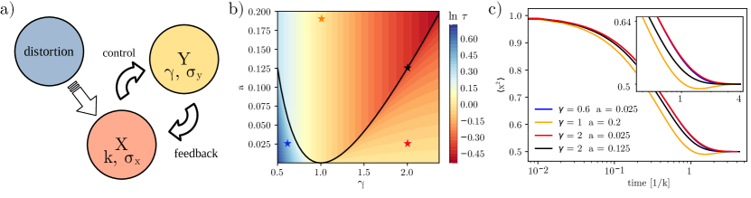
Figure 1: (a) Schematic of feedback adaptation mechanism between $x_{t}$ and $y_{t}$. (b) Relaxation timescale $\tau$ on a logarithmic scale as a function of $a$ and $\gamma$. The black line denotes $a(\gamma)=(k-\gamma)^{2}/4\gamma$. The stars highlights the points considered in panel (c). (c) Evolution of $\langle x_{t}^{2}\rangle$ for several values of $\gamma$ and $a$ (see starts in (b)). The initial state was chosen as $\langle x_{0}^{2}\rangle=\langle y^{2}_{0}\rangle=1$ and $\langle x_{0}y_{0}\rangle=-0.1$ and we set $k=1$, $\sigma_{x}=1$ and $\sigma_{y}=\sigma_{x}/\sqrt{ka}$. The inset shows a magnification of the large-time region.

The relaxation time $\tau$ is shown in Fig. 1b as a function of $a$ and $\gamma$. In the non-interacting scenario $a=0$ the subsystem $x_{t}$ relaxes on the timescale $1/k$ and $y_{t}$ on the timescale $\tau=2/(k+\gamma)=1$. For $\gamma<k$ the timescale increases (blue region in Fig. 1b) and here the feedback loop is not able to accelerate the relaxation. Only for high values of $a$ and $\gamma$ we observe a significant relaxation acceleration (red region in Fig. 1b). An important set of $a,\gamma$ is the line $(k-\gamma)^{2}-4a\gamma=0$ (Fig. 1b, black curve). Above this line, the eigenvalues in Eq. (6) become complex, which may create oscillatory transients with frequency $\omega=[a\gamma-(k-\gamma)^{2}]^{1/2}/2$ during the relaxation of the whole system. The time evolution of the dispersion of the controlled species $x_{t}$, $\langle x_{t}^{2}\rangle$, is shown in Fig. 1c for several values of $\gamma$ and $a$ highlighted in Fig. 1b as stars. For $\gamma=2$, $a=0.025$ as well as $\gamma=0.6$, $a=0.025$ the relaxation rates are similar, since $x_{t}$ is essentially freely relaxing. Conversely, for $\gamma=1$, $a=0.2$ the relaxation occurs in the region where eigenvalues are complex, with relaxation time $\tau=1$ and frequency $\omega=\sqrt{0.2}\approx 0.44$, the oscillations are hence strongly damped (see inset in Fig. 1c). The pair $\gamma=2$, $a=0.125$ is taken on the black curve and displays a faster relaxation and without any oscillations.

II.1 Adaptation of the cellular thermostat

It is a common theme in biology that systems are able to remain in (or close to) homeostasis despite persistent perturbations [6, 31], a process referred to as adaptation. In the case of the cellular thermostat adaptation refers to determining the region of parameters $\gamma,a$ and $\sigma_{y}$, for which $x_{t}$ evolves exactly into the desired homeostatic state $\langle x^{2}\rangle_{\rm eq}=\sigma_{x}^{2}/2k$. Once this region has been determined, any perturbation can be suppressed by increasing $\alpha$ and $\gamma$ along the restricted values. The region of adapted parameters can be determined from Eq. (2), by solving the set of algebraic equations $\textbf{v}_{\rm s}=(\sigma_{x}^{2}/2k,0,\langle y^{2}\rangle_{\rm eq})^{T}=-M^{-1}\textbf{d}$ for $\gamma,a$ and $\sigma_{y}$. Note that we are imposing no constraints on the final distribution of $y_{t\to\infty}$, so the system is not completely determined. We address this problem in Appendix A, where we prove that the constraint

$$\sigma_{y}^{2}=\frac{\sigma_{x}^{2}}{ka}$$ (7)

implies the required adaptation $\langle x^{2}\rangle_{\rm eq}=\sigma_{x}^{2}/2k$. In this case, both $\gamma$ and $a$ remain undetermined, and $\langle y^{2}\rangle_{\rm eq}=\gamma\sigma_{y}^{2}/2=\gamma\sigma_{x}^{2}/2ka$. As an illustrative example we consider the condition Eq. (7) in the relaxation processes in Fig. 1c and confirm that different evolution parameters indeed yield the same final state.

We quantify the velocity of adaptation process in terms of the adaptation error

$$\epsilon(a,\gamma,t)=|\langle x_{t}^{2}\rangle-\langle x^{2}\rangle_{\rm s}|,$$ (8)

which quantifies how far $x_{t}$ from $\langle x^{2}\rangle_{\rm eq}$ at a given time $t$. Using Eq. (4) we can rewrite $\epsilon$ as

$$\epsilon(a,\gamma,t)=|\textbf{e}^{T}_{0}{\rm e}^{{Mt}}(\textbf{v}_{0}-\textbf{v}_{\rm eq})|,$$ (9)

with $\textbf{e}_{0}=(1,0,0)^{T}$. It follows that $\epsilon(a,\gamma,t)\rightarrow 0$ when $t\rightarrow 0$ independent of $\alpha$ and $\gamma$. Along the same lines $\varepsilon(a,\gamma,0)$ is only given by our choice of $\langle x_{0}^{2}\rangle$. In any intermediate state, the adaptation error depends on $\alpha$ and $\gamma$, as well as on $\langle y_{0}^{2}\rangle$.

The adaptation error $\epsilon$ is shown in Fig. 2a as a function of $\gamma$ for several values $a$ at fixed time $t=k=1$. According to Fig. 1c $x_{t}$ at this time is not yet completely relaxed. The points represent different values of $a$ and $\gamma$, the blue points satisfy $a<(k-\gamma)^{2}/4k$ and therefore arise in the region with no oscillations (see Fig. 1). The orange points satisfy $a>(k-\gamma)^{2}/4k$ and lie in the non-monotonic relaxation regime. $\epsilon$ remains high for any $a$ and low values of $\gamma$, since there the control $y_{t}$ reacts too slowly to changes of $x_{t}$. Increasing $\gamma$ we improve the control of $x_{t}$, reducing $\epsilon$. The black line coincides with the black line in Fig. 1b and corresponds to $a=(k-\gamma)^{2}/4\gamma$, while the red line contains the points with minimal adaptation error $\epsilon$ for every $\gamma$. The black and red curves coincide for high values of $\gamma$ and differ for low values.

In order to explain this observation, we must take into account the adaptation condition Eq. (7). According to Eq. (7) the final distribution of $y_{t}$ depends on $a$. Therefore, if $\langle y^{2}\rangle_{\rm eq}(\gamma,a)$ moves far from $\langle y_{0}^{2}\rangle$, the complete system requires additional time to adapt. This fact is especially relevant for low values of $a$. We can represent this result by defining

$$a=\frac{\gamma\sigma_{x}^{2}}{2k\langle y^{2}\rangle_{\rm 0}},$$ (10)

which contains all the points satisfying $\langle y^{2}\rangle_{\rm eq}(\gamma,a)=\langle y_{0}^{2}\rangle$. Along this line the system $y_{t}$ requires no extra time to adapt rendering relaxation efficient (see green line in Fig. 2 and note that it coincides with the red line for low values of $\gamma$).

II.2 Adaptation-dissipation trade-off

An important consequence of the adaptation condition (7) is that it leads to a non-equilibrium situation where detailed balance is broken. It implies a entropy production, even in the steady state. Since $\sigma_{y}$ (as parameterized) depends on $a$, decreasing the adaptation error implies an increasing entropy production. The total entropy production can be separated into (non-negative) adiabatic and non-adiabatic contributions [40], the former being defied as

$$\dot{S}_{\rm a}(t)=\int p_{t}(\textbf{x})\left(\frac{\textbf{J}_{\rm s}(\textbf{x})}{p_{\rm s}(\textbf{x})}\right)^{T}\!D^{-1}\!\left(\frac{\textbf{J}_{\rm s}(\textbf{x})}{p_{\rm s}(\textbf{x})}\right)d\textbf{x}\geq 0,$$ (11)

where $\textbf{x}=(x,y)$, $p_{t}(\textbf{x})$ is the joint probability distribution of $x_{t}$ and $y_{t}$, $p_{\rm s}(\textbf{x})\equiv p_{t\to\infty}(\textbf{x})$ is the steady-state probability density. If we define the positive-definite diagonal diffusion matrix $D\equiv{\rm diag}\,(\sigma_{x}^{2}/2,\gamma^{2}\sigma_{y}^{2}/2)$ then the steady-state (i.e. invariant) current of the system in Eq. (1) is given by $\textbf{J}_{\rm s}(x,y)=-A\textbf{x}p_{\rm s}(\textbf{x})-D\nabla p_{\rm s}(\textbf{x})$. Note that the adiabatic entropy production corresponds to the total entropy production in a non-equilibrium steady state.

The non-adiabatic entropy production represents the additional dissipation due to the relaxation during transient [40, 41, 42, 43]. Even if both contributions are non-zero during the relaxation, we will focus on the adiabatic contribution alone. The reason for this choice is that $S_{\rm a}$ encodes thermodynamic forces breaking time-reversal symmetry, that continuously “steer” relaxation to the non-equilibrium rather than the equilibrium steady state. In addition, assuming Gaussian initial distributions Eq. (7), we can rewrite Eq. (11) in a simple way in terms of $\langle x_{t}^{2}\rangle$ and $\langle y_{t}^{2}\rangle$ (see Appendix A.2) as

$$\dot{S}_{\rm a}(t)=\frac{2a}{\sigma_{x}^{2}}(a\langle y_{t}^{2}\rangle+k\langle x_{t}^{2}\rangle)=\textbf{s}^{T}\textbf{v}_{t}.$$ (12)

where $\textbf{s}=[2a/\sigma_{x}^{2}(k,0,a)]^{T}$, and $\textbf{v}_{t}$ is given by Eq. (4). In turn, the adiabatic entropy produced until time $t$ reads

$$\Delta S^{t}_{\rm a} =\int_{0}^{t}\dot{S}_{\rm a}(\tau)d\tau$$

$$=\textbf{s}^{T}\,\left[\textbf{v}_{\rm s}t+M^{-1}\left({\rm e}^{{Mt}}-1\right)(\textbf{v}_{0}-\textbf{v}_{\rm s})\right].$$ (13)

The first term represents the entropy produced in the steady state in the interval $[0,t]$, given by $\textbf{s}^{T}\,\textbf{v}_{\rm s}t=a(1+\gamma/k)t$ which grows linearly with the control parameters $\alpha$ and $\gamma$. The second term represents the additional adiabatic entropy produced during the transient which can be positive or negative but is always larger than $-\textbf{v}_{\rm s}t$. The splitting in Eq. (13) suggests that the thermodynamic cost of the transient is essentially the cost of maintaining the non-equilibrium steady state (as if it were already reached) augmented by the contribution of the transient that depends on the initial condition.

In Fig. 2b we represent $\epsilon$ as a function of $\Delta S_{\rm a}^{t}$ at time $t=1$, for the values of $a$ and $\gamma$ from Fig. 2a.

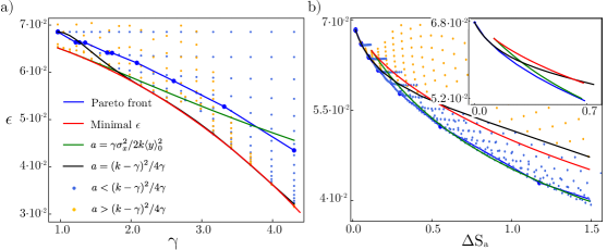
Figure 2: (a) Adaptation error as a function of $\gamma$ for several values of $a\in[10^{-3},2]$ at time $t=1$. Each point represent a different value of $\gamma$ and $a$. Point in orange lie in the oscillatory region, $a>(k-\gamma)^{2}/4k$, the red line represents the result obtained by numerical gradient descent and the blue line is the Pareto front. The black line is given by $a(\gamma)=(k-\gamma)^{2}/4\gamma$ and the green one by $a=\gamma\sigma_{x}^{2}/2k\langle y_{0}^{2}\rangle$. (b) Error rate as a function of the adiabatic entropy change $\Delta S_{\rm a}^{t}$ for the same values of $a$ and $\gamma\in[1,6]$. The color code is the same as in panel (a). Inset: Magnification of the top left region. The initial state was chosen to be $\langle x_{0}^{2}\rangle=\langle y_{0}^{2}\rangle=10$ and $\langle x_{0}y_{0}\rangle=-0.1$. In both panels $k=1$, $\sigma_{x}=1$ and $\sigma_{y}=\sigma_{x}/\sqrt{ka}$.

We observe that all points lie in a region with a convex boundary. This means that we can adjust the parameters $a$ and $\gamma$ to reduce $\epsilon$ until we reach the convex boundary. At this point, decreasing $\epsilon$ always implies an increasing entropy production and vice versa. This boundary is known as the Pareto front, and all the points along the front are called Pareto optimal.

A simple method to determine the Pareto front [21] is via the function

$$J(a,\gamma;\alpha)=\alpha\epsilon(a,\gamma,t)+(1-\alpha)\Delta S_{\rm a}(a,\gamma,t)$$ (14)

where $\alpha\in(0,1)$. The Pareto front $\mathcal{P}$ then corresponds to the set of points $(\gamma,a)(\alpha)$ that minimize $J$ for each $\alpha$

$$\mathcal{P}\equiv\inf_{\gamma,a|\alpha}J(a,\gamma;\alpha)\quad\forall\alpha\in(0,1).$$ (15)

The only requirement for this method to work is that the Pareto front is convex. The presence of a concave region in the Pareto front in the $(\epsilon,\Delta S_{\rm a})$ space in turn implies a sharp jump of the front in the $(\gamma,a)$ space. This fact has been investigated in detail in [21, 18] and will be relevant in the following sections.

In Fig. 2b we determine the Pareto front for the cellular thermostat numerically (blue line). It is completely convex and does not coincide with the red line, since the maximal reduction of $\epsilon$ implies a larger entropy production, pushing the red line away from the front to the right (see Fig. 2b). However, we observe that the structure of the Pareto front is related to the solution sets $a(\gamma)=(k-\gamma)^{2}/4\gamma$ (black line) and $a=\gamma\sigma_{x}^{2}/2k\langle y^{2}\rangle_{\rm 0}$ (green line, Eq. (10)); see inset of Fig. 2b. For low $\Delta S_{\rm a}$, or weak control of $x$, the Pareto front is close to the black line where irreversible driving is more efficient. Increasing $\Delta S_{\rm a}$ the front moves away from the black line and approaches the green line. This reveals that the Pareto optimal solution is given by two different mechanisms: in the left part of Fig. 2b, the Pareto-optimal solution is determined by the more efficient driving, whereas in the right part it is dominated by the lowest dissipation. When both curves coincide, the Pareto front transitions smoothly between the two limiting cases.

We conclude that the shape of the Pareto front is dominated by the solution sets $a(\gamma)=(k-\gamma)^{2}/4\gamma$ and $a=\gamma\sigma_{x}^{2}/2k\langle y^{2}\rangle_{\rm 0}$. These lines characterize the adaptation ability of the feedback cycle and the distance from the initial state, respectively. In Appendix B we provide more data to support the conclusion. There, we consider different initial values and discuss the role of the initial state $\langle y_{0}^{2}\rangle$.

II.3 Adaptation to harmonic perturbations

Molecular process are often subject to periodic perturbations from the environment, for example, by daily light or temperature variations [32, 33]. The biological response to such periodic external modulations is known as circadian rhythms. There exists diverse physiological mechanisms, known as biological clocks, that establish a time-periodic response to external perturbations. Heat-shock proteins are somewhat different, they do not exhibit self-sustained oscillations but are activated by slow time-periodic environmental changes. The daily periodic activation of HSP90 has been found to regulate the behavior of actual biological clocks, which are sensitive to temperature [44]. We focus on the response of the model thermostat to such a time-periodic temperature variation in the long-time limit. We will show that for times larger than the relaxation time, the system reaches a periodic state where the molecule $y$ is continuously activated by the distortion.

We consider that $x$ is subjected to a harmonic temperature variation with frequency $\Omega$, which may represent, e.g. daily temperature oscillations,

$$\sigma_{x}^{2}(t)=\sigma_{x0}^{2}+\delta\cos(\Omega t)$$ (16)

where the amplitude obeys $\delta<\sigma_{x0}^{2}$. Since we are only varying the temperature, the distribution remains a zero-mean Gaussian with a covariance evolving according to

$$\dot{\textbf{v}}_{t}=M\textbf{v}_{t}+\bm{\chi}(t),$$ (17)

where now $\bm{\chi}(t)=\bm{\chi}_{0}+\bm{\chi}_{\rm p}(t)$ is the a sum of a constant part $\bm{\chi}_{0}=(\sigma_{x0}^{2},0,\sigma_{x0}^{2}/ka)$ and a harmonic part $\bm{\chi}_{\rm p}(t)=(\delta\cos(\Omega t),0,\delta\cos(\Omega t)/ka)$. Eq. (17) has the solution

$$\textbf{v}_{t}={\rm e}^{{Mt}}\textbf{v}_{0}+{\rm e}^{{Mt}}\int_{0}^{t}{\rm e}^{{-Mt^{\prime}}}\bm{\chi}(t^{\prime})dt^{\prime}.$$ (18)

We can in turn choose $\sigma_{y}^{2}(t)$ in several ways, depending on how we want to interpret the adaptation in the time-dependent context. The arguably most intuitive (and consistent) choice seems to be to simply impose $\sigma_{y}^{2}(t)=\sigma_{x}^{2}(t)/ka$ at any time, i.e. $y$ up to the amplitude $y$ experiences the same temperature as $x$. Then, the instantaneous quasi-steady state of Eq. (17), given by $0=\dot{\textbf{v}}_{t}=M\textbf{v}^{\rm qs}_{t}+\bm{\chi}(t)$ at any $t$, satisfies $\langle x_{t}^{2}\rangle_{\rm qs}=\sigma_{x}^{2}(t)/2k$ and $\langle y_{t}^{2}\rangle_{\rm qs}=\gamma\sigma_{x}^{2}(t)/2ka$.

We can use the property $\ddot{\bm{\chi}}_{\rm p}(t)=-\Omega^{2}\bm{\chi}_{\rm p}(t)$ to integrate Eq. (18) by parts, yielding

$$\textbf{v}_{t} ={\rm e}^{{Mt}}\textbf{v}_{0}-\left(1-{\rm e}^{{Mt}}\right)M^{-1}\bm{\chi}_{0}$$ (19)

$$+\left(1+\Omega^{2}M^{-2}\right)^{-1}\left[-M^{-1}\bm{\chi}_{\rm p}(t)-M^{-2}\dot{\bm{\chi}}_{\rm p}(t)\right]$$

$$+\left(1+\Omega^{2}M^{-2}\right)^{-1}{\rm e}^{{Mt}}\left[M^{-1}\bm{\chi}_{\rm p}(0)+M^{-2}\dot{\bm{\chi}}_{\rm p}(0)\right].$$

Finally, in the long time regime ${\rm e}^{{Mt}}\overset{t\to\infty}{=}0$ where correlations with the initial state of the system vanish, we obtain

$$\begin{split}\textbf{v}_{t}&\overset{t\to\infty}{=}-M^{-1}\bm{\chi}_{0}\\ &-\left(1+\Omega^{2}M^{-2}\right)^{-1}\left[M^{-1}\bm{\chi}_{\rm p}(t)+M^{-2}\dot{\bm{\chi}}_{\rm p}(t)\right],\end{split}$$ (20)

where the covariance vector $\textbf{v}_{t}$ exhibits an $\Omega$-dependent oscillatory behavior.

For high perturbation frequencies, $\Omega\gg 1$, the second term is $\mathcal{O}(\Omega^{-2})\ll 1$ and the system effectively reaches a stationary state given by $\textbf{v}_{\rm s}\simeq M^{-1}\bm{\chi}_{0}$ with $\langle x^{2}\rangle_{\rm s}=\sigma_{x0}^{2}/2k$ and $\langle y^{2}\rangle_{\rm s}=\gamma\sigma_{x0}^{2}/2ka$. This situation is shown schematically in Fig. 3a (top left).

In the opposite limit, which we refer to as the adiabatic limit, the system is able to perfectly adapt to the environmental perturbations at any time (see Fig. 3a, top right). Precisely, we impose $M^{-2}\to 0$ as well as $\Omega^{2}M^{-2}\to 0$, that is, that the relaxation is fast and in particular much faster than the oscillation period $\Omega^{-1}$. In this adiabatic regime we find $\textbf{v}^{\rm ad}_{t}=-M^{-1}[\bm{\chi}_{0}+\bm{\chi}_{\rm p}(t)]$.

Meanwhile, in the intermediate regime (see Fig. 3a, top center) the adaptation is imperfect and $\langle x_{t}^{2}\rangle$ exhibits a time-periodic evolution with varying amplitude, delayed with respect to the environmental perturbation.

We define the adaptation error analogously to Eq. (8) and rewrite it using Eq. (20) as

$$\begin{split}\epsilon(t)=&|\langle x_{t}^{2}\rangle-\sigma_{x}^{2}(t)/2k|\\ =&\left|\textbf{e}_{0}^{T}\left(1+\Omega^{2}M^{-2}\right)^{-1}M^{-2}\dot{\bm{\chi}_{\rm p}}(t)\right.\\ +&\,\textbf{e}_{0}^{T}\left.\left[\left(1+\Omega^{2}M^{-2}\right)^{-1}-1\right]M^{-1}\bm{\chi}_{\rm p}(t)\right|.\end{split}$$ (21)

As before, the error $\epsilon(t)$ indicates how far the controlled system $x_{t}$ is at time $t$ form the perfectly adapted instantaneous situation. In the adiabatic limit, the adaptation is perfect for any $t$, so $\epsilon(t)=0$. In the limit of high $\Omega$ Eq. (21) instead reduces to

$$\epsilon(t)\overset{\Omega\gg\gamma}{\simeq}|\textbf{e}_{0}^{T}M^{-1}\bm{\chi}_{\rm p}(t)|=\delta/2k|\cos(\Omega t)|.$$ (22)

In the large-time limit the instantaneous adiabatic entropy production in Eq. (12) is also a time-periodic function. The adiabatic entropy produced per period is

$$\dot{\bar{S}}_{\rm a}\equiv\frac{1}{\tau}\int_{0}^{\tau}\dot{S}_{\rm a}(t)dt,$$ (23)

where $\tau=2\pi/\Omega$ is the period of the distortion. Using Eq. (12) in the adiabatic regime we find

$$\dot{\bar{S}}_{\rm a}^{\rm ad}=a\left(1+\frac{\gamma}{k}\right).$$ (24)

Evaluating instead the integral in Eq. (23) in the high-$\Omega$ limit we find

$$\dot{\bar{S}}_{\rm a}\overset{\Omega\gg\gamma}{\simeq}\frac{\dot{\bar{S}}_{\rm a}^{\rm ad}}{\tau}\int_{0}^{\tau}\frac{\sigma_{x0}^{2}}{\sigma_{x}^{2}(t)}dt=\frac{\dot{\bar{S}}_{\rm a}^{\rm ad}}{\sqrt{1-\delta^{2}/\sigma_{x0}^{4}}}\geq\dot{\bar{S}}_{\rm a}^{\rm ad}.$$ (25)

The adiabatic entropy production $\dot{\bar{S}}_{\rm a}$ and adaptation error $\epsilon(\tau=2\pi/\Omega)$ for several values of $\gamma$ and $\Omega$ are shown in Fig. 3a. We observe for $\Omega=20$ and $\gamma\simeq 1$ that both, $\dot{\bar{S}}_{\rm a}$ and $\epsilon(\tau)$ remain close to the high-frequency limit in Eq. (25) with $\epsilon(\tau)=\delta/2k$ (dashed line in Fig. 3a). The high-frequency limit is, however, not reached for smaller values $\Omega=5,2$, since these are comparable to the minimum $\gamma=1$. Increasing $\gamma$ we gradually move into the adiabatic regime in Eq. (24) with $\epsilon(t)=0$ for any $\Omega$. Interestingly, the dependence of $\epsilon(\tau)$ on $\gamma$ is non-monotonic; it exhibits a maximum between the high-$\Omega$ and the adiabatic limits.

In Fig. 3b,c we show $\epsilon(\tau)$ for several values of $a$ and $\gamma$ whereby $\Omega=2$. These results are similar to those in Fig. 2, in particular Fig. 3c reveals a clear border between reachable and impossible values of $\epsilon$ and $\dot{\bar{S}}_{\rm a}$, i.e. the Pareto front. Unlike the example in Fig. 2, the Pareto front here exhibits a concave region at low $\dot{\bar{S}}_{\rm a}$.

The convex part of the front can be reconstructed using the method in Eqs. (14-15), i.e. finding the values of $a$ and $\gamma$ that minimize $J(a,\gamma;\alpha)=\alpha\epsilon(a,\gamma,\tau)+(1-\alpha)\dot{\bar{S}}_{\rm a}(a,\gamma,\tau)$ for $\alpha\in(0,1)$. The results of this method are shown in Fig. 3b,c as points connected by the continuous blue lines. As shown in Fig. 3b, there are in fact three disjoint convex sections: a point (top left), the horizontal line, and the vertical curved line. While the former two are well separated in the $(\epsilon,\gamma)$ space in Fig.3b, they cannot be distinguished in Fig. 3c.

The disjoint sections of the Pareto front reveal distinct underlying optimization mechanisms [21]. The isolated point at $\gamma=1,\epsilon(\tau)=0.125$ represents the limit in which $y$ has no effect on $x$, dissipating no energy. Along the horizontal segment in Fig. 3b the Pareto-optimal solution increases $\gamma$ without improving $\epsilon$ significantly, since the system is stuck in the high-$\Omega$ regime. The vertical segment in Fig. 3b represents the optimization close to the adiabatic regime, where both $\gamma$ and $a$ can be increased to approach the adiabatic regime. The jump between both segments is a result of the non-monotonic dependence of $\epsilon$ on $\gamma$.

Figure 3: (a) Entropy production per cycle $\dot{\bar{S}}_{\rm a}$ relative to the adiabatic limit $\dot{\bar{S}}_{\rm a}^{\rm ad}$ and adaptation error $\epsilon(\tau)$ as a function of $\gamma$ and for several values of $\Omega$. Black dashed lines represent the high-$\Omega$ limit with $\dot{\bar{S}}_{\rm a}^{\rm ad}/\dot{\bar{S}}_{\rm a}=1/\sqrt{1-\delta^{2}/\sigma_{x0}^{4}}\approx 1.15$ and $\epsilon(\tau)=\delta/2k=0.25$. We set $a=(k-\gamma)^{2}/4\gamma$. Top: Schematic of different classes of responses to harmonic distortions; the black line represents the instantaneous value of $\sigma_{x}^{2}(t)$ and the red line the response $\langle x_{t}^{2}\rangle$. (b) Adaptation error $\epsilon$ as a function of $\gamma$ for several values of $a\in[10^{-3},2]$ and $\gamma\in[1,6]$, with $\Omega=2$. The continuous line depicts the Pareto front, dashed lines represent discontinuities of the Pareto front due to concave regions and are merely a guide for the eye. (c) Adaptation error $\epsilon$ as a function of $\dot{\bar{S}}_{\rm a}$ for the same values of $a,\gamma,\Omega$ as in (b). Inset: Magnification of the small-$\dot{\bar{S}}_{\rm a}$ region. The results correspond to $k=\sigma_{x0}^{2}=1$, $\delta=0.5$.

II.4 Stochastic temperature shocks

In certain situations biological processes are continuously stimulated by successive, abrupt changes in environmental conditions at discrete instances of time [31]. Each stimulus triggers the adaptation mechanism during a relaxation period. We now consider the evolution of the concentration $x_{t}$ in such situations.

To represent the random stimulus, we consider again $x_{t}$ following Eq. (1) with time-independent $\sigma_{x}$. At random times $t_{i}$, both $x_{t}$ and $y_{t}$ are instantaneously reset to predefined values distributed according to the probability density $p(x,y)_{\rm res}$. The joint probability density of $x_{t}$ and $y_{t}$ is hence reset at all $t_{i}$ according to $p(x,y;t_{i})\rightarrow p(x,y)_{\rm res}$ and henceforth evolves from $p(x,y)_{\rm res}$. Times $t_{i}$ are ssumed to be Poisson distributed with rate $\Gamma$.

The joint probability density of $x_{t},y_{t}$, $p_{t}(\textbf{x})\equiv p_{t}(x,y)$, follows the extended Fokker-Planck equation [45]

$$\partial_{t}p_{t}(\textbf{x})=-\nabla\cdot\textbf{J}_{t}(\textbf{x})+\Gamma\left[p_{\rm res}(\textbf{x})-p_{t}(\textbf{x})\right],$$ (26)

with $\textbf{J}_{t}(\textbf{x})=-A\textbf{x}p_{t}(\textbf{x})-D\nabla p_{t}(\textbf{x})$ and $A$ given in Eq. (5) and $D\equiv{\rm diag}\,(\sigma_{x}^{2}/2,\gamma^{2}\sigma_{y}^{2}/2)$. The solution $p_{t}(\textbf{x})$ is not Gaussian, not even if we choose a Gaussian resetting density $p_{\rm res}(\textbf{x})$. However, the vector of covariance elements evolves according to

$$\dot{\textbf{v}}_{t}=M\textbf{v}_{t}+\textbf{d}+\Gamma[\textbf{v}_{\rm res}-\textbf{v}_{t}],$$ (27)

where $\textbf{d}\equiv(\sigma_{x}^{2},0,\gamma^{2}\sigma_{y}^{2})^{T}$, the matrix $M$ was defined in Eq. (3), and $\textbf{v}_{\rm res}\equiv(\langle x^{2}\rangle_{\rm res},0,\langle y^{2}\rangle_{\rm res})$ is the covariance of $p_{\rm res}(\textbf{x})$ written in vector form for notational convenience.

In contrast to the previous examples, where we focused on the adaptation during the transient (time-dependent regimes), we here observe how the system reaches a non-equilibrium steady state satisfying

$$\textbf{v}_{\rm NESS}=-(M-\Gamma\mathbb{I})^{-1}(\textbf{d}+\Gamma\textbf{v}_{\rm res}),$$ (28)

with $\mathbb{I}$ being the $3\times 3$ identity matrix. In Appendix A.3 we derive two asymptotic solutions of Eq. (28). For low rates $\Gamma\ll 1$ we have $\textbf{v}^{-}_{\rm NESS}\simeq\textbf{v}_{\rm s}+\Gamma M^{-1}(\textbf{v}_{\rm s}-\textbf{v}_{\rm res})$, i.e. the system remains close to the perfectly adapted state $\textbf{v}_{\rm s}$. Conversely, for large resetting rates $\Gamma\gg 1$, we find $\textbf{v}^{+}_{\rm NESS}\simeq\textbf{v}_{\rm res}+M(\textbf{v}_{\rm res}-\textbf{v}_{\rm s})/\Gamma$, that is, $\textbf{v}_{t}$ is pushed to the reset state $\textbf{v}_{\rm res}$.

We define the adaptation error as

$$\epsilon(a,\gamma) \equiv|\langle x^{2}\rangle_{\rm NESS}-\langle x^{2}\rangle_{\rm s}|$$ (29)

$$=|\textbf{e}_{0}^{T}\left[(M-\Gamma\mathbb{I})^{-1}(\textbf{d}+\Gamma\textbf{v}_{\rm res})+M^{-1}\textbf{d}\right]|,$$

which is time independent. In the two asymptotic regimes we obtain, respectively,

$$\epsilon(a,\gamma) \overset{\Gamma\gg k}{\simeq}\left|\textbf{e}_{0}^{T}\left(\mathbb{I}-M/\Gamma\right)(\textbf{v}_{\rm res}-\textbf{v}_{\rm s})\right|$$ (30)

$$\epsilon(a,\gamma) \overset{\Gamma\ll k}{\simeq}\Gamma\left|\textbf{e}_{0}^{T}M^{-1}(\textbf{v}_{\rm s}-\textbf{v}_{\rm res})\right|.$$ (31)

In the non-equilibrium steady state the total entropy production is time independent and is comprised of $\dot{S}_{\rm a}$ due to the temperature difference between the subsystems and a contribution of the resetting, proportional to $\Gamma$ [45]. However, for a fixed $\Gamma$, only the adiabatic entropy production $\dot{S}_{\rm a}$ plays a relevant role in the trade-off between adaptation and dissipation, such that we may, without loss of generality, consider this contribution only.

As already mentioned, $p_{t}(\textbf{x})$ in Eq. (26) is not Gaussian and Eq. (12) hence does not apply. We evaluate $\dot{S}_{\rm a}$ numerically for a Gaussian $p_{\rm res}(\textbf{x})$, exploiting that between any two consecutive resets at times $t_{i}$ and $t_{i+1}$, the process is indeed Gaussian. The initial condition for each trajectory is drawn from the NESS of the non-reset process. That is, between any such $t_{i}$ and $t_{i+1}$ the adiabatic entropy production follows Eq. (12) with $\textbf{v}_{t_{i}}=\textbf{v}_{\rm res}$. We denote such contributions for a given sample sequence of $\{t_{i}\}(\omega)$ by $\dot{S}_{\rm a}(t|i)$, leading to

$$\Delta S^{t}_{\rm a}(\omega)\equiv\sum_{i=0}^{N(\omega)}\int_{t_{i}}^{t_{i+1}}\dot{S}_{\rm a}(t|i)dt,$$ (32)

where $N(\omega)$ is the number of resets in the sample sequence $\omega$ and we set $t_{N(\omega)+1}\equiv t$. Note that these account for the average over Langevin evolutions (1) between the resets but not yet over different realizations of reset times. We now simulate $10^{3}$ statistically independent trajectories of reset times of length $t=120$ setting $\langle x^{2}\rangle_{\rm res}=\sigma_{x}^{2}/2k$, and $\langle y^{2}\rangle_{\rm res}=\gamma\sigma_{y}^{2}/2$. The adiabatic entropy production in $[0,t]$ then follows as an average over all samples $\Delta S^{t}_{\rm a}=\langle\Delta S^{t}_{\rm a}(\omega)\rangle_{\omega}$.

The results for $\epsilon$ and $\dot{S}^{t}_{\rm a}$ obtained this way are shown in Fig 4a for different values of $\Gamma$. According to the prediction (31), the adaptation error vanishes for low $\Gamma$ and increases monotonically up to $\epsilon=\langle x^{2}\rangle_{\rm res}-\sigma_{x}^{2}/2k=1/2$ for $\Gamma\simeq 100$. Similarly, $\dot{S}^{t}_{\rm a}$ a increases monotonically with $\Gamma$. Interestingly, for low $\Gamma$ we find $\dot{S}^{t}_{\rm a}=0.357$, whereas for high $\Gamma$ we recover $\dot{S}^{t}_{\rm a}=0.56$, corresponding to the Gaussian prediction in Eq. (12) with $\textbf{v}=\textbf{v}_{\rm s}$ and $\textbf{v}=\textbf{v}_{\rm res}$, for the respective limits, suggesting that the limiting distribution is essentially Gaussian.

In Fig. 4b-e we analyze $\epsilon$ and $\dot{S}^{t}_{\rm a}$ for several values of $\gamma$ and $a$ in the intermediate regimes $\Gamma=0.1,30$. In the first case (see Fig. 4b,c) the behavior is similar to that in Fig. 2. Indeed, for low $\Gamma$ the system has enough time to equilibrate upon a reset, and we can explain the Pareto front (blue line) and the lowest error curve (red line) using the curves $a=(k-\gamma)^{2}/4\gamma$ (black line) and $a=\gamma\sigma_{x}^{2}/2k\langle y^{2}\rangle_{\rm res}$ (green line), as in the beginning of the section.

The situation changes for $\Gamma=30$ (see Fig. 4d-e), since $x_{t}$ has no time to recover between resetting events and the feedback action of $y_{t}$ is not relevant. In Fig. 2d we observe that the minimum error is obtained when $y_{t}$ is reset into its own equilibrium state (i.e. the green and red lines in Fig. 2d coincide). The Pareto front is again determined by defining $J(a,\gamma;\alpha)\equiv\alpha\epsilon(a,\gamma)+(1-\alpha)\dot{S}^{t}_{\rm a}(a,\gamma)$ and finding the minima for $\alpha\in(0,1)$. In Fig. 2e we observe that the front is convex in the entire parameter space, and coincides $\gamma=1$ with the optimal entropy production (black curve in Fig. 2e). In Fig. 2d we find that the Pareto front becomes vertical at $\gamma=4$, indicating that the lower part of the front in Fig. 2e is bounded by the limiting maximum value $\gamma=4$. In this case, the Pareto front depends on our choice of the parameter space, so one could continue improving the solutions by increasing $\gamma$.

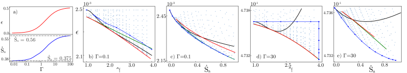
Figure 4: (a) Adaptation error and adiabatic entropy production on $[0,t]$ as a function of $\Gamma$ for $\gamma=2$ and $a=(k-\gamma)^{2}/4\gamma$. (b-e) Adaptation error as a function of $\gamma$ and $\dot{S}^{t}_{a}$ for $\Gamma=0.1$ (b-c) and $30$ (d-e). Each point represent a different value of $a\in[10^{-3},2]$ and $\gamma\in[1,4]$. Red lines denote the minimal adaptation error, the blue curves are the Pareto fronts, and black and green curves are defined by $a=(k-\gamma)^{2}/4\gamma$ and $a=\gamma\sigma_{x}^{2}/2k\langle y^{2}\rangle_{0}$, respectively. The remaining parameters are the same as in Fig. 2.

III Kinetic proofreading in receptor-ligand reactions

A correct protein synthesis requires a precise recognition of correct amino acids at their respective enzymatic sites in the ribosome. However, many amino acid are similar, giving rise to synthesis errors. More generally, substrates can react with different undesired ligand molecules at the same time, creating spurious complex products. Proofreading networks are one possible a solution to this central problem in molecular biology [4]. These networks represent the binding of an amino acid (or more generally ligand) to the enzyme (referred to as the receptor) to create the protein (generally the complex) coupled to an ATP-hydrolysis reaction. The hydrolysis reaction provides a free energy input to drive the ligand binding out-of-equilibrium, promoting binding of correct ligands [4, 5]. The mechanism is referred to as kinetic proofreading and is sketched in Fig. 5a [5].

We study the adaptation of a model proofreading network upon a change of concentration of the ligand converted to a fixed amount of the complex. We determine optimal solutions to the adaptation-dissipation trade-off, revealing distinct mechanisms underlying optimal solutions. We consider the reversible reaction between a receptor $R$ and the ligand $L$ to create a complex $R_{L}$. The activation of this complex is coupled to the hydrolysis of ATP (denoted $T$) to ADP (denoted $D$), $R_{L}+T\rightarrow R_{L}^{*}+D$. In this section, we will consider the transient initiated when ligand $L$ arrives to $R$. When this happens, the network relaxes into an adapted state defined by the concentration of $R_{L}$. The velocity of the relaxation into the adapted state is given by the reaction rates $k_{1,2,3}$ and the concentrations of $T,D$ and $L$. With a slight abuse (albeit simplification) of notation we use $T,D$ and $L$ to denote the concentrations of the respective molecules.

We assume the environment to be at constant temperature, and moreover consider chemostated (i.e. constant) concentrations of $L,D$ and $T$. The evolution of the probability (or concentration) of receptor and both complex states follows the master equation $\dot{\textbf{p}}_{t}=M_{\rm R}\textbf{p}_{t}$ with [5]

$$M_{\rm R}\equiv\left(\begin{matrix}-Lk^{+}_{1}-Lk^{-}_{3}&k^{-}_{1}&k^{+}_{3}\\ Lk^{+}_{1}&-Tk^{+}_{2}-k^{-}_{1}&Dk^{-}_{2}\\ Lk^{-}_{3}&Tk^{+}_{2}&-Dk^{-}_{2}-k^{+}_{3}\end{matrix}\right)$$ (33)

where $\textbf{p}_{t}=[p_{R}(t),p_{R_{L}}(t),p_{R_{L}^{*}}(t)]^{T}$ is the probability of the respective states at time $t$, normalized according to $p_{R}(t)+p_{R_{L}}(t)+p_{R_{L}^{*}}=1$. The species inter-convert with chemical rates $k^{+}_{i}$, $i=1,2,3$ as denoted by the black arrows in Fig. 5a. The reverse reactions occur with rates $k^{-}_{i}=k^{+}_{i}\exp(\beta\Delta\mu_{i})$, where $1/\beta$ is the environmental temperature. $\Delta\mu_{i}$ is the chemical potential difference of each reaction, satisfying $\Delta\mu_{1}+\Delta\mu_{2}+\Delta\mu_{3}=0$. The total chemical potential driving the reaction is

$$\beta\Delta\mu=\ln\left(T/D\right).$$ (34)

In contrast to the feedback system in the previous section, which was driven by a temperature difference, the thermodynamic driving force here is the concentration difference between $T$ and $D$. If $T=D$ the system evolves towards thermal equilibrium with $p_{R}^{\rm eq},p_{R_{L}}^{\rm eq},p_{R_{L}^{*}}^{\rm eq}$ satisfying the detailed balance conditions, $p_{R_{L}}^{\rm eq}/p_{R}^{\rm eq}=\exp(-\beta\Delta\mu_{1}),p_{R_{L}^{*}}^{\rm eq}/p_{R_{L}}^{\rm eq}=\exp(-\beta\Delta\mu_{2})$ and $p_{R}^{\rm eq}/p_{R_{L}^{*}}^{\rm eq}=\exp(-\beta\Delta\mu_{3})$, independently of $L$. If, however, $\Delta\mu\neq 0$, the hydrolysis reaction will create steady-state currents in the reaction cycle, with a sign dictated by the relative concentrations of $T$ and $D$. These currents produce entropy proportional to $\Delta\mu$ [5].

III.1 Adaptation

The stationary probabilty distribution of the network is set by the concentration of $R_{L}$, and must be independent of other parameters of the dynamics. We choose the adaptation condition

$$p_{R_{L}}^{\rm st}/p_{R}^{\rm st}=\phi=\rm{const.}$$ (35)

where $\phi$ is a fixed parameter. Imposing $\dot{\textbf{p}}_{t}=0$ and inserting Eq. (35) into the master equation we obtain the following relation between $L$, $T$ and $D$

$$\frac{L}{\phi}=\frac{k^{-}_{1}k^{+}_{3}+Dk^{-}_{1}k^{-}_{2}+Tk_{3}^{+}k^{+}_{2}}{k^{+}_{1}k^{+}_{3}+Dk^{+}_{1}k^{-}_{2}+Dk^{-}_{3}k^{-}_{2}},$$ (36)

i.e.  the constant concentrations of $T$ and $D$ determine the concentration of $L$ that is required to satisfy the condition in Eq. (35).

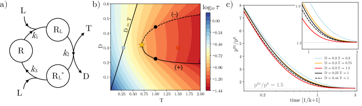
Figure 5: (a) Schematic of the chemical reaction network performing kinetic proofreading. (b) $\log_{10}\tau$ (color bar) as a function of $T$ and $D$. The black lines are given by $D_{+}(T)$, $D_{-}(T)$ and $D=T$. The blue and red circles and the star represent the points used considered in panel c. (c) Probability ratio $P_{R_{L}}(t)/P_{R}(t)$ for several values of $T$ and $D$. The inset shows a magnification of the long-time regime. We used $\phi=1.5$, $\beta=1$, $k^{+}_{1}=k^{+}_{2}=k^{+}_{3}=1$, $\Delta\mu_{1}=\Delta\mu_{3}=-0.5$ and $\Delta\mu_{1}=1$. $L$ is given by Eq. (36). $p_{R}(0)=0.1$, $p_{R_{L}}(0)=0.9$ and $p_{R_{L}}(0)=0$.

The solution of the master equation is $\textbf{p}_{t}={\rm e}^{{M_{R}t}}\textbf{p}_{0}$, where $M_{R}$ is defined in Eq. (5). The matrix $M_{\rm R}$ has one zero eigenvalue, whose right eigenvector is the steady-state probability already described by Eq (35). The remaining two eigenvalues, $\lambda_{+}$ and $\lambda_{-}$ describe the evolution during the transient. Their real parts $\rm{Re}[\lambda_{\pm}]<0$ are negative, whereas the imaginary parts $\rm{Im}[\lambda_{\pm}]$ may (but does not need to) be different from zero. If it is non-zero, it gives rise to oscillations during the transient.

The relaxation timescale of the transient is given by $\tau=1/\min(\rm{Re}[\lambda_{+}],\rm{Re}[\lambda_{-}])$ and is shown in Fig. 5b (on a logarithmic scale) for several values of $T$ and $D$. It depends explicitly on $\phi$ due to Eq. (35). The full and dashed black lines denoted by $(\pm)$ represent concentrations for which $\rm{Im}[\lambda_{\pm}]$ becomes different from zero, and enclose the region of oscillatory transients. From Fig. 5b we conclude that, increasing $T$ above $D$ accelerates adaptation by shortening the transient. This gives rise to a clockwise steady-state circulation in the reaction cycle in Fig. 5a. Counter-clockwise oscillations imply moving across the line $D=T$ and only marginally improve $\tau$. For low values of $T$ and $D$, the timescale $\tau$ decays along the $D=T$ line due to the increasing concentration of $L$.

The system’s adaptation speed to $\phi=1.5$ is shown in Fig. 5c for several values of $T$ and $D$ denoted in Fig. 5b with red/blue points and a star. The initial condition is $p_{R}(0)=0.1$, $p_{R_{L}}(0)=0.9$ and $p_{R_{L}}(0)=0$. Notably, we observe no discernible oscillations for parameters chosen within the nominally oscillatory region where $\rm{Im}[\lambda_{\pm}]\neq 0$.

III.2 Adaptation-dissipation trade-off

As before we characterize the adaptation accuracy in terms of the adaptation error here defined as

$$\epsilon(T,D;t)=|p_{R_{L}}(t)/p_{R}(t)-\phi|$$ (37)

at any time $t$. For times much larger than the relaxation time $t\gg\tau$ the system adapts to the desired steady state such that $\epsilon\to 0$. In the following, we consider the error at $t=1/k^{+}_{1,2,3}=1$, when the system is not yet completely relaxed as seen in Fig. 5c.

To describe dissipation, we consider the adiabatic entropy production rate, given by [46]

$$\dot{S}_{\rm a}(T,D;t)=\sum^{3}_{i,j=1}M_{R}^{ij}(\mathbf{p}_{t})_{j}\ln\left(\frac{M_{R}^{ij}(\mathbf{p}^{\rm st})_{j}}{M_{R}^{ji}(\mathbf{p}^{\rm st})_{i}}\right)\geq 0.$$ (38)

where $(\textbf{p}_{t})_{i}$ for $i=1,2,3$ are the components of $\textbf{p}_{t}$ and $\mathbf{p}^{\rm st}=\textbf{p}_{t\to\infty}$. The entropy production rate is positive during the transient as well as in the non-equilibrium steady state. It only vanishes at equilibrium, attained for $T=D$ for which detailed balance holds.

The adaptation error $\epsilon(t=1)$ is shown in Fig. 6 as a function of the concentration of $T$ and $\Delta S_{\rm a}$ for several values of $T,D\in[0,5]$. Protein-synthesis process are intermittent [47]; we thus consider the initial concentrations to be $p_{R}(0)=0.9$, $p_{R_{L}}(0)=0.1$ and $p_{R_{L}}^{*}(0)=0$, i.e. the absence of the complex prior to the arrival of the ligand. The black lines correspond to the curves $(\pm)$ in Fig. 5b and the red line to points with $T=D$. For low $T$, $\epsilon(1)$ decays fastest close to the detailed-balance case (red curve). In this regime, the adaptation is accelerated due to an increasing $L$ at $\Delta\mu=0$. Upon increasing $T$, the detailed-balance curve saturates and there is not further reduction of the adaptation error. In this regime of $T$, the adaptation error decreases fastest along the $(+)$ line, in agreement with the relaxation time in Fig. 5b. For this set of parameters $\Delta\mu>0$ grows, giving rise to strong clockwise currents in the network.

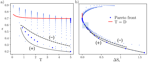
Figure 6: Adaptation error as a function of (a) $T$ and (b) $\Delta S_{\rm a}$ in the chemical reaction network from Fig. 5a. Blue dots represent different values of $T,D\in[0,5]$, the solid and dashed black lines the $(\pm)$ curves in Fig. 5b, the red line corresponds to $T=D$, and the blue curve is the Pareto front. The blue square indicates the region where the Pareto front becomes concave. The initial condition is $p_{R}(0)=0.9$, $p_{R_{L}}(0)=0.1$ and $p_{R_{L}}(0)=0$. Other parameters are the same as in Fig. 5.

The parameter set $T=D$ satisfies detailed balance and therefore the red line falls into the low-entropy-production region (see Fig. 6b). The curves $(\pm)$ are quite similar; along the $(+)$ line the adaptation error becomes reduced maximally, whereas along the $(-)$ line $\Delta\mu$ is smaller (see Fig. 5b).

In the convex domain the Pareto front is determined as before, by finding the values of $T$ and $D$ that minimize

$$\mathcal{P}\!=\!\inf_{T,D|\alpha}[\alpha\epsilon(T,D;t)+(1-\alpha)\Delta S(T,D;t)],\,\,\forall\alpha\in(0,1),$$ (39)

i.e.  each point in the Pareto front corresponds to a single value of $\alpha$. The Pareto front obtained via Eq. (39) is shown in Fig. 6b (blue line). It contains two convex sections. In the region indicated by a blue square, we observe a concave section, whose consequences are echoed in Fig. 6a, where we observe that the convex sections of the Pareto front are in fact completely disjoint. One section coincides with the detailed-balance regime $T=D$, the other with the $(+)$ line. This reveals the existence of two distinct optimization mechanisms that we have already hypothesized based on intuition. In the concave section, these mechanism are said to coexist[18, 21]. Along the detailed-balance line $T=D$, the system only poorly improves $\epsilon$, but with the advantage of zero adiabatic dissipation, since the adaptation condition Eq. (36) can always be met for growing $L$. Along the $(+)$ line, the system is very efficient in reducing $\epsilon$, albeit at the expense of producing increasing amounts of entropy. The relation between the Pareto front and the region with complex eigenvalues, is similar to that in Fig. 2.

IV Conclusion

We investigated the adaptation ability of two biologically relevant model systems, the cellular thermostat and a minimal ATP-driven receptor-ligand reaction network. In the context of the thermostat, we considered how the synthesis and back-action of heat/cold-shock proteins regulates the effective temperature experienced by proteins under different environmental conditions (a single temperature shock, time-periodic temperature cycles, and stochastic temperature shocks). In the context of receptor-ligand reactions we focused on how the relaxation speed and terminal state of the formed complex upon the change in ligand concentration are affected by the coupling to an ATP-hydrolysis reaction that is in turn controlled by the difference between ATP and ADP concentrations.

We analyzed the adaptation accuracy of both systems and determined the respective Pareto fronts, i.e. optimal solutions to the trade-off between adaptation accuracy and dissipation. These solutions do not optimize adaptation, but instead determine a compromise between the adaptation error and entropy production. Their structure depends on the particular external disruption, and may contain one or more convex sections along the front. Each convex section is associated with a particular optimization mechanism, while in the concave sections Pareto optimality corresponds to the coexistence of distinct mechanisms.

The evolution of living systems has led to highly optimized processes. In this work, we limited the discussion to the structure of optimal process parameters that give rise to compromises between adaptation and thermodynamic cost (i.e. dissipation), and explored some of their consequences. Rather than being rigidly determined, these “compromise-optimal” solutions are distributed along extended fronts in parameter space, endowing biological systems with a great flexibility to evolve, resist, and adapt to very different environments. It is conceivable that the marked changes in response mechanisms observed in experiments [48, 49, 11] may be explained by changes in the adaptation mechanisms along Pareto fronts, since such fronts were shown to exhibit abrupt changes in the response to even the smallest variations in the environment.

V Acknowledgments

Financial support from the Alexander von Humboldt foundation (postdoctoral fellowship to JTB) as well as the German Research Foundation (DFG) through the Heisenberg Program (grant GO 2762/4-1 to AG) and European Research Council (ERC) under the European Union’s Horizon Europe research and innovation program (grant agreement No 101086182 to AG) is gratefully acknowledged.

Appendix A cellular thermostat – dynamics and dissipation

A.1 Steady-state solutions

We write the Lyapunov equation, Eq. (2) in components

$$\begin{split}\frac{d\langle x_{t}^{2}\rangle}{dt}&=-2k\langle x_{t}^{2}\rangle-2a\langle x_{t}y_{t}\rangle+\sigma_{x}^{2},\\ \frac{d\langle x_{t}y_{t}\rangle}{dt}&=-(\gamma+k)\langle x_{t}y_{t}\rangle+\gamma\langle x_{t}^{2}\rangle-a\langle y_{t}^{2}\rangle,\\ \frac{d\langle y_{t}^{2}\rangle}{dt}&=-2\gamma\langle y_{t}^{2}\rangle+2\gamma\langle x_{t}y_{t}\rangle+\gamma^{2}\sigma_{y}^{2},\end{split}$$ (A1)

whose steady state is given by $\frac{d}{dt}\langle x_{t}^{2}\rangle=\frac{d}{dt}\langle x_{t}y_{t}\rangle=\frac{d}{dt}\langle y_{t}^{2}\rangle=0$ which yields Eq. (2), i.e.

$$\langle y^{2}\rangle_{\rm s}=\frac{2\langle xy^{2}\rangle_{\rm s}+\gamma\sigma_{y}^{2}}{2},$$ (A2)

as well as

$$\langle xy\rangle_{\rm s}=\frac{\gamma}{a+k+\gamma}\left(\langle x^{2}\rangle_{\rm s}-\frac{a\sigma^{2}_{y}}{2}\right),$$ (A3)

and finally also

$$2k\langle x^{2}\rangle_{\rm s}=\sigma_{x}^{2}-\frac{2a\gamma}{a+k+\gamma}\left(\langle x^{2}\rangle_{\rm s}-\frac{a\sigma^{2}_{y}}{2}\right).$$ (A4)

The steady-state values depend on $\gamma$, $a$, $\sigma_{x}$ and $\sigma_{y}$. The adapted state satisfies the condition $\langle x^{2}\rangle_{\rm s}=\sigma_{x}^{2}/2k$, implying the constraint $\sigma_{y}^{2}=\sigma_{x}^{2}/ka$. Under this constraint we in turn find $\langle xy\rangle_{\rm s}=0$ and $\langle y^{2}\rangle_{\rm s}=\gamma\sigma_{y}^{2}/2$.

A.2 Adiabatic entropy production

The adiabatic component of the total entropy production rate, Eq. (11), simplifies for Gaussian states as follows. An instantaneous Gaussian state is defined by the probability density

$$p_{t}(\textbf{x})=\mathcal{N}_{t}{\rm e}^{{-\textbf{x}^{T}\Sigma_{t}^{-1}\textbf{x}/2}},$$ (A5)

where $\Sigma$ is the time-dependent correlation matrix and $\mathcal{N}_{t}$ is a normalization factor. In the steady state, once we impose Eq. (7), we have

$$p_{\rm s}(\textbf{x})\equiv p_{t\to\infty}(\textbf{x})=\mathcal{N}_{\rm s}\exp\left(-\frac{kx^{2}}{\sigma_{x}^{2}}-\frac{y^{2}}{\gamma\sigma_{y}^{2}}\right),$$ (A6)

where from follows the steady-state current

$$\textbf{J}_{\rm s}(\textbf{x})=-\left(\begin{matrix}0&-a\\ \gamma&0\\ \end{matrix}\right)\textbf{x}\rho_{\rm s},$$ (A7)

and finally from Eq. (11) also the adiabatic entropy production in Eq. (11)

$$\dot{S}_{\rm a}(t)=\frac{2a}{\sigma_{x}^{2}}(a\langle y_{t}^{2}\rangle+k\langle x_{t}^{2}\rangle).$$ (A8)

A.3 Steady state under stochastic temperature shocks

Here we analyze the cellular thermostat under continuous-time stochastic temperature shocks, in the limit of large and small shock (i.e. resetting) rate $\Gamma$. Recall that the extended Fokker-Planck equation reads

$$\partial_{t}p_{t}(\textbf{x})=\nabla\cdot\left[A\textbf{x}p_{t}(\textbf{x})\!+\!D\nabla p_{t}(\textbf{x})\right]+\Gamma\left[p_{\rm res}(\textbf{x})\!-\!p_{t}(\textbf{x})\right].$$ (A9)

A.3.1 Small-$\Gamma$ limit

For small $\Gamma$ we can expand the solution perturbatively in orders of $\Gamma$

$$p_{t}(\textbf{x})=\Gamma^{0}p_{t}^{(0)}(\textbf{x})+\Gamma p_{t}^{(1)}(\textbf{x})+\Gamma^{2}p_{t}^{(2)}(\textbf{x})+...$$ (A10)

Inserting back to Fokker-Planck equation and collecting matching orders of $\Gamma$ we obtain the hierarchy of equations

$$\partial_{t}p_{t}^{(0)}\! =\!\nabla\cdot\!\left[A\textbf{x}p_{t}^{(0)}(\textbf{x})+D\nabla p_{t}^{(0)}\textbf{x})\right]$$ (A11)

$$\partial_{t}p_{t}^{(1)}\! =\!\nabla\cdot\!\left[A\textbf{x}p_{t}^{(1)}(\textbf{x})+D\nabla p_{t}^{(1)}(\textbf{x})\right]\!+\!\left[p_{\rm res}(\textbf{x})\!-\!p_{t}^{(0)}(\textbf{x})\right]$$

$$\partial_{t}p_{t}^{(2)}\! =\!\nabla\cdot\!\left[A\textbf{x}p_{t}^{(2)}(\textbf{x})+D\nabla p_{t}^{(2)}(\textbf{x})\right]\!-\!p_{t}^{(1)}(\textbf{x})$$

$$\partial_{t}p_{t}^{(3)}\! =\!\nabla\cdot\!\left[A\textbf{x}p_{t}^{(3)}(\textbf{x})+D\nabla p_{t}^{(3)}(\textbf{x})\right]\!-\!p_{t}^{(2)}(\textbf{x})$$

$$\vdots$$

$$\partial_{t}p_{t}^{(n)}\! =\!\nabla\cdot\!\left[A\textbf{x}p_{t}^{(n)}(\textbf{x})+D\nabla p_{t}^{(n)}(\textbf{x})\right]\!-\!p_{t}^{(n-1)}(\textbf{x}).$$

If the initial distribution is Gaussian we can evaluate the covariance elements to any order $n$ in $\Gamma$, $\textbf{v}_{t}^{(n)}=(\langle x_{t}^{2}\rangle^{(n)},\langle x_{t}y_{t}\rangle^{(n)},\langle y_{t}^{2}\rangle^{(n)})$ as

$$\dot{\textbf{v}}_{t}^{(0)} =M\textbf{v}_{t}^{(0)}+\textbf{d}$$ (A12)

$$\dot{\textbf{v}}_{t}^{(1)} =M\textbf{v}_{t}^{(1)}+\textbf{d}+\textbf{v}_{\rm res}-\textbf{v}_{t}^{(0)}$$

$$\dot{\textbf{v}}_{t}^{(2)} =M\textbf{v}_{t}^{(2)}+\textbf{d}-\textbf{v}_{t}^{(1)}$$

$$\vdots$$

$$\dot{\textbf{v}}_{t}^{(n)} =M\textbf{v}_{t}^{(n)}+\textbf{d}-\textbf{v}_{t}^{(n-1)},$$

where $\textbf{d}\equiv(\sigma_{x}^{2},0,\gamma^{2}\sigma_{y}^{2})^{T}$. In the steady state, we can solve the system of algebraic equations $\dot{\textbf{v}}_{t}^{(n)}=0$ for all $n$

$$\begin{split}\textbf{v}^{(0)}=&-M^{-1}\textbf{d}\\ \textbf{v}^{(n)}=&-M^{-n}\textbf{v}_{\rm res}-\sum_{i=0}^{n}M^{-i-1}\textbf{d}\\ =&-M^{-n}\textbf{v}_{\rm res}-M^{-1}(\mathbbm{I}-M^{-1})^{-1}(\mathbbm{I}-M^{-n-1})\textbf{d},\end{split}$$ (A13)

and evaluate the covariance vector $\textbf{v}_{\rm NESS}=\textbf{v}_{0}+\textbf{v}_{1}\Gamma+...$ yielding

$$\textbf{v}_{\rm NESS}= -M^{-1}\textbf{d}-\sum_{n=1}^{\infty}\Gamma^{n}\left(M^{-n}\textbf{v}_{\rm res}+\sum_{i=0}^{n}M^{-i-1}\textbf{d}\right)$$

$$= -M^{-1}\textbf{d}-\Gamma M^{-1}(\mathbbm{I}-\Gamma M^{-1})^{-1}\textbf{v}_{\rm res}$$ (A14)

$$-\frac{\Gamma}{1-\Gamma}M^{-1}(\mathbbm{I}-M^{-1})^{-1}\textbf{d}$$

$$+\Gamma M^{-3}(\mathbbm{I}-M^{-1})^{-1}(\mathbbm{I}-\Gamma M^{-1})^{-1}\textbf{d},$$

and the convergence of the sums is guaranteed by taking $\Gamma$ small enough to ensure $\lim_{n\to\infty}(\Gamma M^{-1})^{n}=0$. To the first order in $\Gamma$ we obtain

$$\textbf{v}_{\rm NESS}=\textbf{v}_{\rm s}+\Gamma M^{-1}(\textbf{v}_{\rm s}-\textbf{v}_{\rm res})+\mathcal{O}(\Gamma^{2}),$$ (A15)

which was considered in the main part.

A.3.2 Large-$\Gamma$ limit

For high $\Gamma$ we set $\varepsilon\equiv 1/\Gamma$ and expand as

$$p_{t}(\textbf{x})=\varepsilon^{0}\bar{p}_{t}^{(0)}(\textbf{x})+\varepsilon\bar{p}_{t}^{(1)}(\textbf{x})+\varepsilon^{2}\bar{p}_{t}^{(2)}(\textbf{x})+...$$ (A16)

and collect orders of $\varepsilon$

$$\partial_{t}\bar{p}_{t}^{(0)}\! =\!\nabla\cdot\!\left[A\textbf{x}\bar{p}_{t}^{(0)}(\textbf{x})+D\nabla\bar{p}_{t}^{(0)}\textbf{x})\right]-\bar{p}_{t}^{(1)}(\textbf{x})$$

$$\partial_{t}\bar{p}_{t}^{(1)}\! =\!\nabla\cdot\!\left[A\textbf{x}\bar{p}_{t}^{(1)}(\textbf{x})+D\nabla\bar{p}_{t}^{(1)}(\textbf{x})\right]\!+\!\left[p_{\rm res}(\textbf{x})\!-\!\bar{p}_{t}^{(2)}(\textbf{x})\right]$$

$$\partial_{t}\bar{p}_{t}^{(2)}\! =\!\nabla\cdot\!\left[A\textbf{x}\bar{p}_{t}^{(2)}(\textbf{x})+D\nabla\bar{p}_{t}^{(2)}(\textbf{x})\right]\!-\!\bar{p}_{t}^{(3)}(\textbf{x})$$

$$\partial_{t}\bar{p}_{t}^{(3)}\! =\!\nabla\cdot\!\left[A\textbf{x}\bar{p}_{t}^{(3)}(\textbf{x})+D\nabla\bar{p}_{t}^{(3)}(\textbf{x})\right]\!-\!\bar{p}_{t}^{(4)}(\textbf{x})$$

$$\vdots$$

$$\partial_{t}\bar{p}_{t}^{(n)}\! =\!\nabla\cdot\!\left[A\textbf{x}\bar{p}_{t}^{(n)}(\textbf{x})+D\nabla\bar{p}_{t}^{(n)}(\textbf{x})\right]\!-\!\bar{p}_{t}^{(n+1)}(\textbf{x}).$$

Again, for a Gaussian initial condition we find

$$\dot{\bar{\textbf{v}}}_{t}^{(0)} =-M\bar{\textbf{v}}_{t}^{(0)}+\textbf{d}-\bar{\textbf{v}}_{t}^{(1)}$$

$$\dot{\bar{\textbf{v}}}_{t}^{(1)} =-M\bar{\textbf{v}}_{t}^{(1)}+\textbf{d}+\textbf{v}_{\rm res}-\bar{\textbf{v}}_{t}^{(2)}$$

$$\dot{\bar{\textbf{v}}}_{t}^{(2)} =-M\bar{\textbf{v}}_{t}^{(2)}+\textbf{d}-\bar{\textbf{v}}_{t}^{(3)}$$ (A17)

$$\vdots$$

$$\dot{\bar{\textbf{v}}}_{t}^{(n)} =-M\bar{\textbf{v}}_{t}^{(n)}+\textbf{d}-\bar{\textbf{v}}_{t}^{(n+1)},$$

and the steady-state follows straightforwardly, once we identify $\textbf{v}_{0}=\textbf{v}_{\rm res}$ (i.e. the limit $\Gamma\to\infty$) yielding,

$$\bar{\textbf{v}}^{(0)}= \textbf{v}_{\rm res},$$ (A18)

$$\bar{\textbf{v}}^{(1)}= -M\textbf{v}_{\rm res}+\textbf{d}$$

$$\vdots$$

To first order in $\Gamma^{-1}$ we thus obtain

$$\textbf{v}_{\rm NESS}=\textbf{v}_{\rm res}+M(\textbf{v}_{\rm res}-\textbf{v}_{\rm s})/\Gamma+\mathcal{O}(\Gamma^{-2}),$$ (A19)

which is used in the main part.

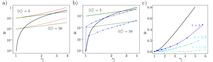
Figure A1: (a) Minimal adaptation error (red lines) and (b) Pareto front (blue) during relaxation of the cellular thermostat at time $t=1$ for two different values of $\langle y^{2}_{0}\rangle$ shown in the $\gamma,\alpha$ space. In both (a) and (b) he black line represents $a=(k-\gamma)^{2}/4\gamma$ curve and the green one corresponds to $a=\gamma\sigma_{x}^{2}/2k\langle y^{2}_{0}\rangle$ [see Eq. (10)]. (c) Pareto fronts in the $\gamma,\alpha$ space at different times during relaxation of the cellular thermostat; the black line denotes $a=(k-\gamma)^{2}/4\gamma$. The remaining parameters are taken as in Fig. (1)

Appendix B Additional information on the cellular thermostat

Here we provide additional data supporting the results from the main text. We consider the cellular thermostat during the relaxation process in Fig. 1c.

Results for the minimal adaptation error (corresponding to the red lines shown in Fig. 2) for two different values of $\langle y_{0}^{2}\rangle$ are shown in Fig. A1a. The green lines correspond to $a=\gamma\sigma_{x}^{2}/2k\langle y_{0}^{2}\rangle$ and contain information about the initial state of $y$. In Fig. A1b we show Pareto fronts corresponding to the blue lines in Fig. 2. We observe how the blue and red lines vary with $\langle y_{0}^{2}\rangle$. The black line in Fig. A1 corresponds to $a=(k-\gamma)^{2}/4\gamma$ and coincides with the black line in Fig. 1b and, notably, does not depend on $\langle y_{0}^{2}\rangle$.

In Fig. A1c we show Pareto fronts in the $\gamma,\alpha$ space at several times during relaxation. The black line corresponds again to $a=(k-\gamma)^{2}/4\gamma$. At early times, the Pareto front remains close to $a=0$ because the feedback mechanism has no time to reduce the adaptation error $\epsilon(t=0.1)$, and the unique optimal solution corresponds to reducing dissipation. At larger times, the feedback system becomes more efficient, and the Pareto front moves closer to the black line. Increasing $t$ implies a reduction of the adaptation error.

References

- Astumian and Hänggi [2002] R. D. Astumian and P. Hänggi, Brownian Motors, Phys. Today 55, 33 (2002).
- Astumian [2019] R. D. Astumian, Kinetic asymmetry allows macromolecular catalysts to drive an information ratchet, Nat. Commun. 10, 1 (2019).
- Amano et al. [2022] S. Amano, M. Esposito, E. Kreidt, D. A. Leigh, E. Penocchio, and B. M. W. Roberts, Insights from an information thermodynamics analysis of a synthetic molecular motor, Nat. Chem. 14, 530 (2022).
- Boeger [2022] H. Boeger, Kinetic Proofreading, Annu. Rev. Biochem. , 423 (2022).
- Qian [2007] H. Qian, Phosphorylation Energy Hypothesis: Open Chemical Systems and Their Biological Functions, Annu. Rev. Phys. Chem. , 113 (2007).
- Ma et al. [2009] W. Ma, A. Trusina, H. El-Samad, W. A. Lim, and C. Tang, Defining Network Topologies that Can Achieve Biochemical Adaptation, Cell 138, 760 (2009).
- Smirnakis et al. [1997] S. M. Smirnakis, M. J. Berry, D. K. Warland, W. Bialek, and M. Meister, Adaptation of retinal processing to image contrast and spatial scale, Nature 386, 69 (1997).
- Hazelbauer et al. [2008] G. L. Hazelbauer, J. J. Falke, and J. S. Parkinson, Bacterial chemoreceptors: high-performance signaling in networked arrays, Trends Biochem. Sci. 33, 9 (2008).
- Thieringer et al. [1998] H. A. Thieringer, P. G. Jones, and M. Inouye, Cold shock and adaptation, BioEssays 20, 49 (1998).
- Etchegaray et al. [1996] J.-P. Etchegaray, P. G. Jones, and M. Inouye, Differential thermoregulation of two highly homologous cold-shock genes, and , of, Genes Cells 1, 171 (1996).
- Buckley et al. [2001] B. A. Buckley, M.-E. Owen, and G. E. Hofmann, Adjusting the thermostat: the threshold induction temperature for the heat-shock response in intertidal mussels (genus Mytilus) changes as a function of thermal history, J. Exp. Biol. 204, 3571 (2001).
- Sriram et al. [2012] K. Sriram, M. Rodriguez-Fernandez, and F. J. D. Iii, A Detailed Modular Analysis of Heat-Shock Protein Dynamics under Acute and Chronic Stress and Its Implication in Anxiety Disorders, PLoS One 7, e42958 (2012).
- Sivéry et al. [2016] A. Sivéry, E. Courtade, and Q. Thommen, A minimal titration model of the mammalian dynamical heat shock response, Phys. Biol. 13, 066008 (2016).
- Schmiedl and Seifert [2007] T. Schmiedl and U. Seifert, Optimal Finite-Time Processes In Stochastic Thermodynamics, Phys. Rev. Lett. 98, 108301 (2007).
- Falasco et al. [2022] G. Falasco, M. Esposito, and J.-C. Delvenne, Beyond thermodynamic uncertainty relations: nonlinear response, error-dissipation trade-offs, and speed limits, J. Phys. A: Math. Theor. 55, 124002 (2022).
- Guéry-Odelin et al. [2023] D. Guéry-Odelin, C. Jarzynski, C. A. Plata, A. Prados, and E. Trizac, Driving rapidly while remaining in control: classical shortcuts from Hamiltonian to stochastic dynamics, Rep. Prog. Phys. 86, 035902 (2023).
- Plata et al. [2020] C. A. Plata, D. Guéry-Odelin, E. Trizac, and A. Prados, Finite-time adiabatic processes: Derivation and speed limit, Phys. Rev. E 101, 032129 (2020).
- Solon and Horowitz [2018] A. P. Solon and J. M. Horowitz, Phase Transition in Protocols Minimizing Work Fluctuations, Phys. Rev. Lett. 120, 180605 (2018).
- Censor [1977] Y. Censor, Pareto optimality in multiobjective problems, Appl. Math. Optim. 4, 41 (1977).
- Shoval et al. [2012] O. Shoval, H. Sheftel, G. Shinar, Y. Hart, O. Ramote, A. Mayo, E. Dekel, K. Kavanagh, and U. Alon, Evolutionary Trade-Offs, Pareto Optimality, and the Geometry of Phenotype Space, Science 336, 1157 (2012).
- Seoane and Solé [2016] L. F. Seoane and R. Solé, Multiobjective Optimization and Phase Transitions, in Proceedings of ECCS 2014 (Springer, Cham, Switzerland, 2016) pp. 259–270.
- Barato and Seifert [2015a] A. C. Barato and U. Seifert, Thermodynamic Uncertainty Relation for Biomolecular Processes, Phys. Rev. Lett. 114, 158101 (2015a).
- Barato and Seifert [2015b] A. C. Barato and U. Seifert, Universal Bound on the Fano Factor in Enzyme Kinetics, J. Phys. Chem. B 119, 6555 (2015b).
- Seifert [2019] U. Seifert, From Stochastic Thermodynamics to Thermodynamic Inference, Annu. Rev. Condens. Matter Phys. , 171 (2019).
- Gingrich et al. [2016] T. R. Gingrich, J. M. Horowitz, N. Perunov, and J. L. England, Dissipation bounds all steady-state current fluctuations, Phys. Rev. Lett. 116, 120601 (2016).
- Horowitz and Gingrich [2019] J. M. Horowitz and T. R. Gingrich, Thermodynamic uncertainty relations constrain non-equilibrium fluctuations, Nat. Phys. 16, 15–20 (2019).
- Seifert [2018] U. Seifert, Stochastic thermodynamics: From principles to the cost of precision, Physica A 504, 176 (2018), lecture Notes of the 14th International Summer School on Fundamental Problems in Statistical Physics.
- Hartich and Godec [2021] D. Hartich and A. Godec, Thermodynamic uncertainty relation bounds the extent of anomalous diffusion, Phys. Rev. Lett. 127, 080601 (2021).
- Dieball and Godec [2023] C. Dieball and A. Godec, Direct route to thermodynamic uncertainty relations and their saturation, Phys. Rev. Lett. 130, 087101 (2023).
- Proesmans [2023] K. Proesmans, Precision-dissipation trade-off for driven stochastic systems, Commun. Phys. 6, 10.1038/s42005-023-01343-5 (2023).
- Lan et al. [2012] G. Lan, P. Sartori, S. Neumann, V. Sourjik, and Y. Tu, The energy–speed–accuracy trade-off in sensory adaptation, Nat. Phys. 8, 422 (2012).
- Mehra et al. [2006] A. Mehra, C. I. Hong, M. Shi, J. J. Loros, J. C. Dunlap, and P. Ruoff, Circadian Rhythmicity by Autocatalysis, PLoS Comput. Biol. 2, e96 (2006).
- Dobroborsky [2006] B. Dobroborsky, Thermodynamics of biological systems, North-Western State Medical University Press: Saint-Petersburg, Russia (2006).
- Pigllucci [1996] M. Pigllucci, How organisms respond to environmental changes: from phenotypes to molecules (and vice versa), Trends in Ecology & Evolution 11, 168 (1996).
- Marchler and Wu [2001] G. Marchler and C. Wu, Modulation of Drosophila heat shock transcription factor activity by the molecular chaperone DROJ1, EMBO J. 10.1093/emboj/20.3.499 (2001).
- Feldman and Frydman [2000] D. E. Feldman and J. Frydman, Protein folding in vivo: the importance of molecular chaperones, Curr. Opin. Struct. Biol. 10, 26 (2000).
- Tu et al. [2008] Y. Tu, T. S. Shimizu, and H. C. Berg, Modeling the chemotactic response of Escherichia coli to time-varying stimuli, Proc. Natl. Acad. Sci. U.S.A. 105, 14855 (2008).
- Sartori et al. [2014] P. Sartori, L. Granger, C. F. Lee, and J. M. Horowitz, Thermodynamic Costs of Information Processing in Sensory Adaptation, PLoS Comput. Biol. 10, e1003974 (2014).
- Conti and Mora [2022] D. Conti and T. Mora, Nonequilibrium dynamics of adaptation in sensory systems, Phys. Rev. E 106, 054404 (2022).
- Van den Broeck and Esposito [2010] C. Van den Broeck and M. Esposito, Three faces of the second law. II. Fokker-Planck formulation, Phys. Rev. E 82, 011144 (2010).
- Dieball et al. [2023] C. Dieball, G. Wellecke, and A. Godec, Asymmetric thermal relaxation in driven systems: Rotations go opposite ways, Phys. Rev. Res. 5, L042030 (2023).
- Ibáñez et al. [2024] M. Ibáñez, C. Dieball, A. Lasanta, A. Godec, and R. A. Rica, Heating and cooling are fundamentally asymmetric and evolve along distinct pathways, Nat. Phys. 20, 135–141 (2024).
- Dieball and Godec [2024] C. Dieball and A. Godec, Thermodynamic bounds on generalized transport: From single-molecule to bulk observables, Phys. Rev. Lett. 133, 067101 (2024).
- Goda et al. [2014] T. Goda, B. Sharp, and H. Wijnen, Temperature-dependent resetting of the molecular circadian oscillator in Drosophila, Proc. R. Soc. B. 281, 10.1098/rspb.2014.1714 (2014).
- Mori et al. [2023] F. Mori, K. S. Olsen, and S. Krishnamurthy, Entropy production of resetting processes, Phys. Rev. Res. 5, 023103 (2023).
- Esposito and Van den Broeck [2010] M. Esposito and C. Van den Broeck, Three faces of the second law. I. Master equation formulation, Phys. Rev. E 82, 011143 (2010).
- Depken et al. [2013] M. Depken, J. M. R. Parrondo, and S. W. Grill, Intermittent Transcription Dynamics for the Rapid Production of Long Transcripts of High Fidelity, Cell Rep. 5, 521 (2013).
- Bettencourt et al. [2002] B. R. Bettencourt, I. Kim, A. A. Hoffmann, and M. E. Feder, Response To Natural And Laboratory Selection At The Drosophila Hsp70 Genes, Evolution 56, 1796 (2002).
- Hoffmann and Harshman [1999] A. A. Hoffmann and L. G. Harshman, Desiccation and starvation resistance in Drosophila: patterns of variation at the species, population and intrapopulation levels, Heredity 83, 637 (1999).