A Diffusion-based Xray2MRI Model: Generating Pseudo-MRI Volumes From one Single X-ray

Abstract

Knee osteoarthritis (KOA) is a prevalent musculoskeletal disorder, and X-rays are commonly used for its diagnosis due to their cost-effectiveness. Magnetic Resonance Imaging (MRI), on the other hand, offers detailed soft tissue visualization and has become a valuable supplementary diagnostic tool for KOA. Unfortunately, the high cost and limited accessibility of MRI hinders its widespread use, leaving many patients with KOA to rely solely on X-ray imaging. In this study, we introduce a novel diffusion-based Xray2MRI model capable of generating pseudo-MRI volumes from a single X-ray image. In addition to using X-rays as conditional input, our model integrates target depth, KOA probability distribution, and image intensity distribution modules to guide the synthesis process, ensuring that the generated corresponding slices accurately correspond to the anatomical structures. Experimental results demonstrate that by integrating information from X-rays with additional input data, our proposed approach is capable of generating pseudo-MRI sequences that approximate real MRI scans. In addition, by increasing the number of inference steps, the model achieves effective interpolation, which further improves the continuity and smoothness of the generated MRI sequences, representing a promising first attempt at cost-effective medical imaging solutions. This study is available on https://zwang78.github.io/.

Keywords Knee osteoarthritis  $\cdot$ X-ray  $\cdot$ Magnetic Resonance Imaging  $\cdot$ Diffusion-based

1 Introduction

Knee OsteoArthritis (KOA) is a progressive disease marked by the degeneration and damage of articular cartilage, changes at the joint margins, and reactive hyperplasia of the subchondral bone [1]. Various factors, such as age, obesity, stress, and trauma, can contribute to its development [2]. Those affected often endure severe pain and limited mobility, which can greatly diminish their quality of life and elevate the risk of chronic conditions like cardiovascular disease [3]. Despite extensive research, the precise cause of KOA remains unknown, and there is currently no cure [4].

Traditionally, X-ray imaging has been the most common method for diagnosing KOA due to its accessibility and ability to reveal changes in bone structure, such as Joint Space Narrowing (JSN) and osteophyte formation [5]. To assess KOA on X-rays, five distinct grades (i.e., from G-0 to G-4), determined by the presence and severity of symptoms, are commonly used [6]. However, X-ray imaging has limitations, particularly in visualizing soft tissue structures and early cartilage changes. Magnetic Resonance Imaging (MRI), on the other hand, provides a more comprehensive assessment of the knee joint by offering detailed images of both bone and soft tissues, including cartilage, menisci, and synovium [7]. MRI can detect early signs of KOA that are not visible on X-rays, such as bone marrow lesions, synovitis, and early cartilage degeneration [8]. However, the widespread adoption of MRI in the clinical management of KOA is hindered by several challenges, most notably the high cost associated with MRI scans [9]. The expense of MRI technology, including the costs of the equipment, maintenance, and specialized personnel, makes it less accessible compared to traditional X-ray imaging [10]. This economic barrier is particularly significant in resource-limited settings and for patients without adequate health insurance coverage. In addition to the high financial cost, MRI scans require more time and patient cooperation, as they necessitate the patient to remain still for extended periods [11], which can be difficult for those experiencing severe pain or limited mobility due to KOA.

To address these limitations, researchers have explored various techniques to enhance MRI reconstruction and reduce its dependency on traditional methods. Fessler et al. [12] provides an in-depth review of iterative algorithms used for improving MRI image reconstruction, particularly in scenarios where traditional inverse Fourier transforms are inadequate. The author highlights the limitations of conventional methods, especially when dealing with non-Cartesian sampling, under-sampled data, or the presence of nonlinear magnetic fields, and then focuses on model-based approaches, which utilize iterative methods that incorporate physical models of MRI acquisition, allowing for better image quality by addressing inhomogeneity and under-sampling issues. The authors demonstrate that model-based methods can significantly enhance image reconstruction, providing superior results compared to traditional techniques, though often at the cost of increased computation. In [13], Han et al. proposed leveraging the k-space to improve the efficiency and accuracy of MRI reconstruction. The authors introduced a framework inspired by the low-rank Hankel matrix completion approach, which directly interpolates missing k-space data and enhances the representation of MRI data by learning the underlying signal structure, resulting in high-quality images even from undersampled data. The proposed k-space deep learning approach significantly reduces the computational complexity and memory requirements. In [14], Lustig et al. leveraged compressed sensing to significantly accelerate MRI scan times without compromising image quality. The authors explore the inherent sparsity of MR images, both in the image domain and in transform domains. By randomly undersampling k-space and using nonlinear recovery schemes, the study shows that high-quality MR images can be reconstructed from incomplete data. This approach effectively reduces acquisition time and mitigates artefacts that arise from undersampling, which demonstrates that compressed sensing has the potential to substantially reduce scan times in clinical settings, making MRI more efficient and accessible.

With the rapid advancements in deep learning technologies, the field of MRI reconstruction has seen significant growth [15] [16]. Recently, combining multi-modal and diffusion-based models has become a new trend for image generation. In [17], Zhan et al. presented a novel medical generative model, MedM2G, designed to unify multiple medical modalities (e.g., CT, MRI, X-ray) and tasks (e.g., text-to-image, image-to-text, modality translation) into a single, efficient framework. The authors address the challenge of aligning and generating medical multi-modal data, particularly in the absence of large, well-paired datasets. They propose a central alignment strategy to efficiently align different modalities using text as the central modality and introduce medical visual invariant preservation to retain key clinical knowledge from each modality. The model leverages a multi-flow cross-guided diffusion process that facilitates adaptive interaction among modalities, enhancing the generation of accurate and high-quality medical images. In [18], Jiang et al. introduced a novel diffusion-based approach to multi-modal MRI synthesis. Traditional diffusion models for MRI synthesis typically operate in the original image domain, leading to high memory consumption and less effective handling of anatomical structures. CoLa-Diff addresses these challenges by operating in the latent space to reduce memory overhead while preserving anatomical details. The model introduces structural guidance using brain region masks and an auto-weight adaptation mechanism to balance multiple input modalities effectively during synthesis. The authors demonstrate that CoLa-Diff outperforms existing state-of-the-art models in multi-modal MRI synthesis tasks, showing superior results in terms of Peak Signal-to-Noise Ratio (PSNR) and Structural Similarity Index (SSIM). In [19], Kim et al. propose an advanced method for translating MRI images between different modalities. The authors introduce an Adaptive Latent Diffusion Model (ALDM) that leverages a novel multiple-switchable spatially adaptive normalization (MS-SPADE) block to transform source latent representations into target-like latent. This approach enables high-quality image synthesis across multiple modalities without requiring patch cropping, preserving the global information of the images. By conditioning the model with target modalities and applying the ALDM in a compressed latent space, the proposed method significantly reduces computational complexity while achieving superior results in both one-to-one and one-to-many image translation tasks.

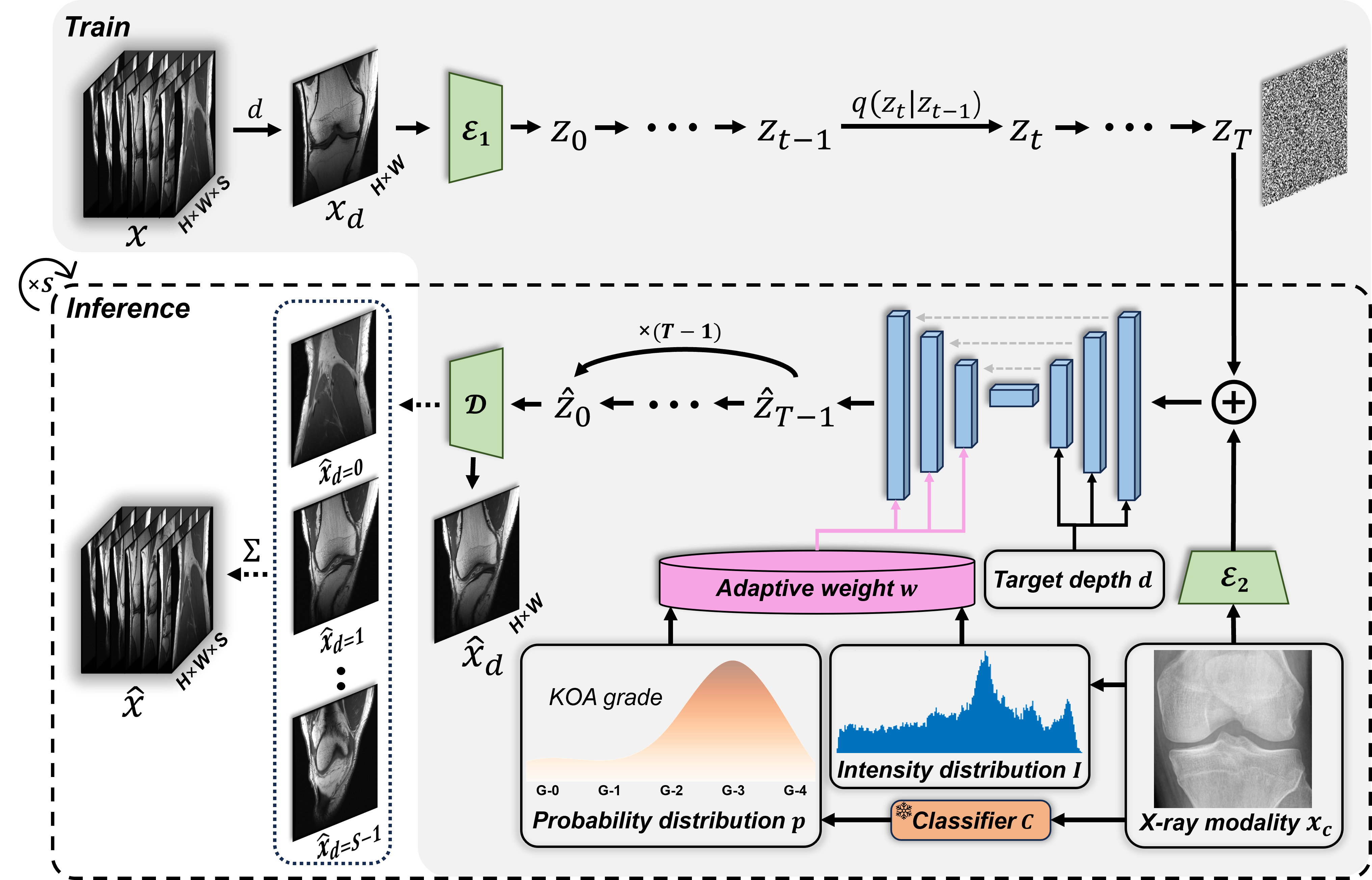
Inspired by the above work, we propose a novel approach named Xray2MRI, based on the Conditional Latent Diffusion Model (CLDM) [20]. Specifically, during the training phase, each real MRI slice is first noised and then progressively denoised using the corresponding X-ray as conditional input and the adaptive-weight guidance of the target depth, image intensity distribution, and KOA probability distribution to reconstruct the input MRI slice. In the inference phase, given a knee X-ray and a target depth, the model progressively denoises from Gaussian noise to generate the corresponding MRI slice at that depth. Then, the target depth is adjusted and the denoising process is repeated iteratively for each depth until all the required slices are synthesized. These individual slices are then stacked together to form a full 3D MRI volume. It is noteworthy that the reconstructed MRI is not intended to serve as a clinical replacement for a real MRI. Still, it marks a pioneering cross-modal attempt to generate corresponding pseudo-MRI volumes from X-rays, for seeking cost-effective medical imaging solutions.

The primary contributions of this paper include the following:

• A novel CLDM-based framework, named Xray2MRI, is proposed to generate pseudo-MRI volumes from a single X-ray image.

• In addition to the target depth, information about KOA probability distribution and image intensity distribution from the X-ray is combined via an adaptive-weight module to guide the denoising process.

• A new SSIM-based evaluation metric is specially developed. The multi-indicator assessment approach ensures both quantitative and qualitative validation of the synthesized MRI images for both image quality and clinical relevance.

• The model demonstrates effective interpolation between MRI slices by increasing the number of inference steps (i.e., exceeding the depth of the original MRI volume), resulting in smoother transitions and improved continuity between the generated slices.

2 Proposed approach

2.1 Classical conditional latent diffusion model

Before delving into the proposed approach, we provide a brief overview of the classic conditional latent diffusion model, which serves as the foundation for our methodology.

Figure 1: The structure of the classical conditional latent diffusion model.

Figure 2: The flowchart of the proposed approach, starts by extracting a slice at position $d$ from a real MRI sequence $x$, denoted as $x_{d}$. This slice is encoded by the encoder $\mathcal{E}_{1}$ to produce a latent representation $z_{0}$, which is progressively noised following the distribution $q(z_{t}|z_{t-1})$, ultimately generating the noised latent representation $z_{T}$. The corresponding X-ray image $x_{c}$ is then used as a conditional input, encoded by $\mathcal{E}_{2}$, and concatenated with $z_{T}$ to form the initial input for the downsampling network. During the denoising process, the target depth $d$ is embedded at various stages of the downsampling phase. Concurrently, the KOA probability distribution $p$, obtained from a pre-trained KOA classifier $\mathcal{C}$, and the image intensity distribution $i$ from the X-ray image are integrated into the upsampling phase through an adaptive weighting module, providing dynamic guidance. This denoising process is repeated for $T-1$ iterations to progressively refine the latent representation, resulting in the denoised latent $\hat{z}_{0}$, which is decoded by $\mathcal{D}$ to reconstruct the MRI slice $\hat{x}_{d}$ at depth $d$. During inference, the process begins with $z_{T}$ and is repeated $S$ times, corresponding to the number of channels $S$ in the original MRI sequence. Finally, the full pseudo-MRI sequence $\hat{x}$ is obtained by stacking all the generated MRI slices in sequential order (i.e., $\hat{x}$ = $\{\hat{x}_{d=1}$, $\hat{x}_{d=2}$,…,$\hat{x}_{d=S}\}$).

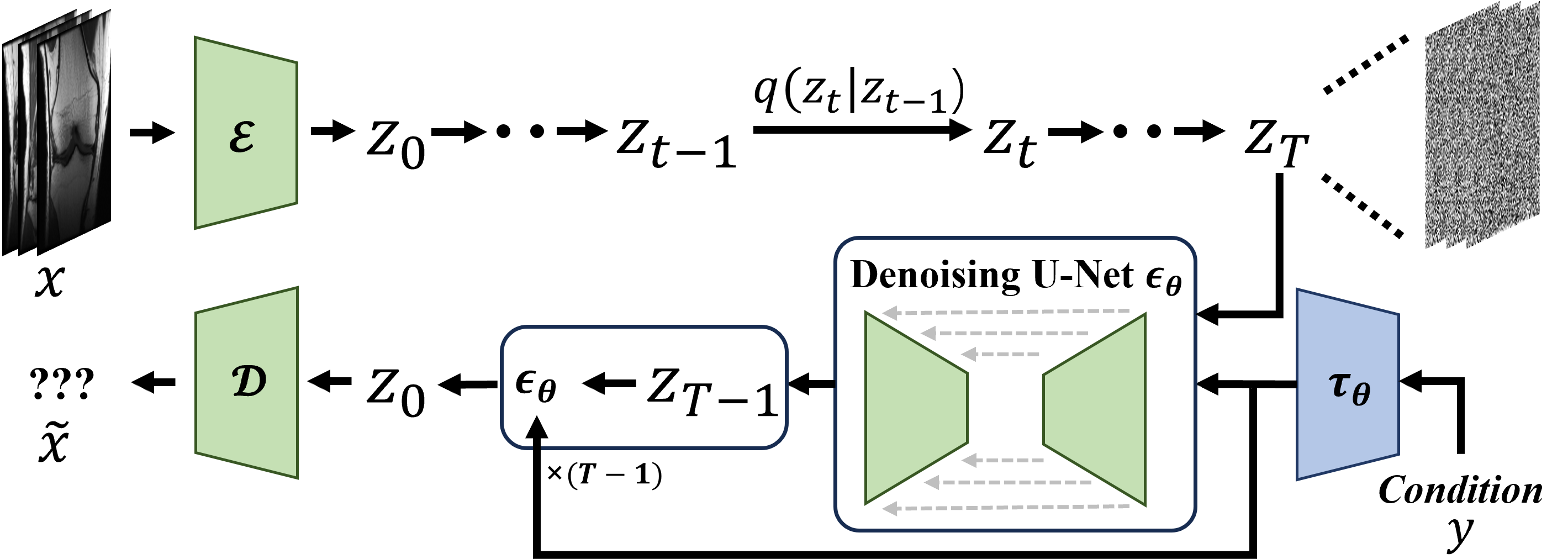
As shown in Fig. 1, a conditional latent diffusion model is a type of generative model used for producing data (such as images, audio, or text) based on certain conditions or inputs. This model combines the strengths of diffusion models and latent variable models, allowing it to generate complex data distributions while being guided by specific conditions. Different modules are to be introduced, respectively.

2.1.1 Encode process

The latent variable model is used to map the input image $x$ to a latent space using an encoder:

$$z_{0}=\mathcal{E}(x)$$ (1)

where $\mathcal{E}$ is an encoder which maps an image $x$ to a latent representation $z_{0}$.

2.1.2 Diffusion process

A diffusion process describes the evolution of a random variable over time. Through the forward diffusion process, for the original latent representation $z_{0}\sim q(z_{0})$, each step of the diffusion process, which comprises a total of $T$ steps, involves adding Gaussian noise $n$ to the data obtained from the previous step $z_{t-1}$ as follows:

$$q(z_{t}\mid z_{t-1})=\mathcal{N}(z_{t};\sqrt[]{1-\beta_{t}}z_{t-1},\beta_{t}\mathbf{I})$$ (2)

where $\beta_{t}$ represents the variance used for each step in the range of $[0,1]$, and $\mathbf{I}$ represents the identity matrix. The entire diffusion process constitutes a Markov chain [21]:

$$q(z_{1}\mid z_{0})=\prod_{t=1}^{T}q(z_{t}\mid z_{t-1})$$ (3)

Here, we directly sample $z_{t}$ for any step $t$ based on the original data $z_{0}$: $z_{t}\sim q(z_{t}\mid z_{0})$ defining $\alpha_{t}=1-\beta_{t}$ and $\bar{\alpha}t=\prod{i=1}^{t}\alpha_{i}$. Through the reparameterization technique, we have:

$$z_{t} =\sqrt{\alpha_{t}}z_{t-1}+\sqrt{1-\alpha_{t}}\epsilon_{t-1}$$ (4)

$$=\sqrt{\alpha_{t}}(\sqrt{\alpha_{t-1}}z_{t-2}+\sqrt{1-\alpha_{t-1}}\epsilon_{t-2})+\sqrt{1-\alpha_{t}}\epsilon_{t-1}$$

$$=\sqrt{\bar{\alpha}_{t}}z_{0}+\sqrt{1-\bar{\alpha}_{t}}\epsilon,\quad\quad\forall\epsilon_{t}\sim\mathcal{N}(0,\mathbf{I})$$

2.1.3 Denoising process

After the diffusion process, denoising is performed by sampling from the updated noise distribution. Estimating distribution $q(x_{t-1}\mid x_{t})$ requires the utilization of the entire training set. Typically, a neural network, such as a U-Net [22], is employed to estimate these distributions. Here, the reverse process is also defined as a Markov chain composed of a sequence of Gaussian distributions parameterized by neural network parameters:

$$p_{\theta}(z_{t-1}\mid z_{t},x_{c})=\mathcal{N}(z_{t-1};\mu_{\theta}(z_{t},t,x_{c}),\sigma_{\theta}^{2}(t))$$ (5)

where $p_{\theta}(z_{t-1}\mid z_{t},x_{c})$ represents parameterized Gaussian distributions, the mean $\mu_{\theta}(z_{t},t,x_{c})$ and variance $\sigma_{\theta}^{2}(t)$ at each time step with the condition $x_{c}$ are determined by trained learning networks.

2.1.4 Training process

The encoder-decoder and diffusion modules are trained separately. For the encoder-decoder, the reconstruction loss $\mathcal{L}_{rec}$ is as:

$$\mathcal{L}_{rec}=||(x,\mathcal{D}(\mathcal{E}(x))||_{2}^{2}$$ (6)

The parameters $\theta$ of the diffusion module aim to minimize the distance between the true noise $\epsilon$ and the predicted noise $\epsilon_{\theta}$. The diffusion loss $\mathcal{L}_{diff}$ quantifies this difference as the expected value of the squared norm between the actual noise and the noise estimated by the neural network:

$$\mathcal{L}_{diff}=\mathbb{E}_{z_{0}\sim\mathcal{E}(x),x_{c},t,\epsilon\sim\mathcal{N}(0,\mathbf{I})}||\epsilon-\epsilon_{\theta}(z_{t},t,x_{c})||_{2}^{2}$$ (7)

where $\mathbb{E}$ represents the expectation over all data points under the joint distribution of the conditioning information $x_{c}$, time steps $t$, and Gaussian noise $\epsilon$.

2.2 Proposed approach

As presented in Fig. 2, our approach consists of three main modules: an auto-encoder module, a CLDM module, and a guidance module. $x_{d}$ is a slice of the original knee MRI sequence $x$ at the depth position $d$ with the size of $H\times W\times S$. $\mathcal{E}_{1}$ and $\mathcal{D}$ are encoder and decoder of the AutoencoderKL [23]. Unlike traditional autoencoders that map input data to a deterministic latent space, the AutoencoderKL introduces a probabilistic approach by encoding the input into a Gaussian distribution over the latent space. During training, the Kullback-Leibler (KL) divergence is used as a regularization term to ensure that the learned latent space closely follows a standard normal distribution, promoting smoother and more continuous transitions between latent representations. Specifically, the encoder operates at a resolution of 256$\times$256$\times$3 and begins with a convolutional layer configured with 128 channels and then proceeds through a series of stages, each with 2 residual blocks. The channel dimensions are multiplied according to the sequence 1, 2, 4, and 4. The decoder mirrors the structure of the encoder. The architecture is designed with no dropout, focusing on retaining all features without stochastic regularization during training. Simultaneously, the noised latent code $z_{T}$ is calculated following Eq. 4:

$$z_{T}=\sqrt{\bar{\alpha_{t}}}\mathcal{E}_{1}({x_{d}})+\sqrt{1-\bar{\alpha}_{T}}\epsilon$$ (8)

Conditional image $x_{c}$ is a corresponding X-ray image, which is then encoded by the encoder $\mathcal{E}_{2}$ and concatenated with the $z_{T}$ as the input of the U-Net, serves as the beginning of the reverse process. The employed 2D U-Net architecture adopts a multi-scale hierarchical structure comprising a time embedding module, an encoder module, a middle module, and a decoder module. This UNet model takes 8-channel input and produces 4-channel output, built upon a base channel configuration of 320. The encoder module begins with a 2D convolutional layer featuring a kernel size of 3 and padding of 1, followed by a series of residual blocks with progressively increasing feature dimensions. Each residual block includes multiple convolutional layers, GroupNorm [24] for normalization, the Swish activation function [25] for non-linearity, and optional dropout for regularization. Two residual blocks are employed per downsampling stage, with attention mechanisms activated at resolutions of 4, 2, and 1. The channel count increases across network layers following a multiplier sequence of 1, 2, 4, and 4. The decoder mirrors this structure, utilizing the same residual blocks to progressively upsample feature maps, reducing the number of channels in reverse order while merging them with corresponding encoder feature maps through skip connections. Additionally, the model incorporates 8 attention heads and employs a spatial transformer with a depth of 1, conditioned on a context dimension of 768.

Next, the target depth $d$ was embedded into the downsampling stage to allow the model to condition the latent representation with spatial hierarchy early in the process. This ensures that depth-related features, such as different tissue layers and bone structures, are incorporated from the outset, preserving the anatomical coherence of the volume. In the upsampling stage, the KOA probability distribution $p$ and image intensity distribution $i$ were embedded to guide the synthesis of fine clinical features based on the spatial hierarchy established during downsampling, such as the presence of osteophytes and the size of the joint space. However, since the variation between slices in MRI is not uniform, different slices have varying levels of sensitivity to the guided information. Some slices may require more emphasis on specific anatomical features, while others may need more focus on KOA severity. To address this, we introduce an automatic weight adjustment mechanism that dynamically combines the information from the KOA probability distribution $p$ and the image intensity distribution $i$ to ensure that the final MRI outputs maintain a higher level of accuracy and clinical relevance by properly leveraging the complementary strengths of both distributions. The adaptive-weight module $w$ begins by independently adjusting the weights of $p$ and $i$ using the $L^{2}$-norm, scaled by the learnable parameters $\mu_{p}$ and $\mu_{i}$, respectively:

$$G_{p}=\mu_{p}\|p\|_{2}=\mu_{p}\left(\sum_{m=1}^{h}\sum_{n=1}^{w}(p_{m,n})^{2}+\kappa\right)^{\frac{1}{2}}$$ (9)

$$G_{i}=\mu_{i}\|i\|_{2}=\mu_{i}\left(\sum_{m=1}^{h}\sum_{n=1}^{w}(i_{m,n})^{2}+\kappa\right)^{\frac{1}{2}}$$ (10)

where $h$ and $w$ represent the height and width of the feature maps $p$ and $i$. $p_{m,n}$ and $i_{m,n}$ represent the values of the respective feature maps at the pixel located at row $m$ and column $n$. $\kappa$ is a small constant added to prevent division by zero, typically set to an empirical value of 1e-05.

Next, the calculated weights $G_{p}$ and $G_{i}$ are normalized as follows:

$$\hat{G}_{p}=\frac{G_{p}}{G_{p}+G_{i}+\epsilon},\quad\hat{G}_{i}=\frac{G_{i}}{G_{p}+G_{i}+\epsilon}$$ (11)

where $\epsilon$ is a small positive constant (e.g., 1e-08) added for numerical stability, preventing division by zero.

Then, $p$ and $i$ are adjusted by applying the normalized weights:

$$\tilde{p}=p\left[1+\sigma(\nu_{p}\hat{G}_{p}+o_{p})\right],\quad\tilde{i}=i\left[1+\sigma(\nu_{i}\hat{G}_{i}+o_{i})\right]$$ (12)

where $\sigma$ is a Sigmoid function. $v_{p}$, $v_{i}$, and $o_{p}$, $o_{i}$ are learnable scaling and offset parameters to $p$ and $i$, respectively.

To capture the interaction between $p$ and $i$, a joint condition weight $\lambda_{pi}$ is learned using an attention mechanism [26], which is represented as:

$$\lambda_{pi}=\text{Attention}(p,i)=\text{softmax}\left(\frac{(W_{p}p)^{\top}(W_{i}i)}{\sqrt{p_{k}}}\right)$$ (13)

where $W_{p}$ and $W_{i}$ are learnable weight matrix associated with $p$ and $i$, respectively. $\sqrt{p_{k}}$ is a scaling factor.

The final combined condition $\tilde{y}_{pi}$ with the learned joint condition weight $\lambda_{pi}$ is as follows:

$$\tilde{y}_{pi}=\lambda_{pi}\cdot(\tilde{p}+\tilde{i})$$ (14)

As presented before, the diffusion model is implemented through a U-Net $\mathcal{U}$, which is trained based on Eq. 7. In this study, the goal function is computed as follows:

$$\mathop{\min}_{\theta}\mathbb{E}_{z\sim\varepsilon_{1}(x_{d}),t,\epsilon\sim\mathcal{N}(0,\mathbf{I})}||\epsilon-\epsilon_{\theta}\{z_{t},t,[z_{T},\mathcal{C}(x_{c}),w(p,i)]\}||_{2}^{2}$$ (15)

During the denoising process, the latent variable $z_{t-1}$ is sampled using the Denoising Diffusion Implicit Model (DDIM) [27], which enables deterministic or stochastic generation depending on the chosen schedule. DDIM refines the sampling process by approximating the reverse diffusion trajectory more efficiently than traditional diffusion models. Specifically, it leverages a non-Markovian process that skips some diffusion steps, allowing for faster inference without compromising the quality of the generated images. The sampling of $z_{t-1}$ is computed as follows:

$$z_{t-1}=\sqrt{\bar{\alpha}_{t-1}}\left(\frac{z_{t}-\sqrt{1-\bar{\alpha}_{t}}\mathbf{\epsilon}_{\theta}}{\sqrt{\bar{\alpha}_{t}}}\right)+\sqrt{1-\bar{\alpha}_{t-1}}\mathbf{\epsilon}_{\theta}$$ (16)

Finally, for each reconstructed slice at the depth $d$, denoted as $\hat{x}_{d}$, it is generated through a decoder $\mathcal{D}$. During the inference phase, this process is repeated $S$ times, corresponding to the channel (depth) $S$ of the original MRI volume. The final generated pseudo-MRI sequence $\hat{x}$ is formed by stacking all generated slices, represented as $\hat{x}=\{\hat{x}_{0},\hat{x}_{1},\dots,\hat{x}_{s-1}\}$. For more clarity, Algorithm 1 and Algorithm 2 describe the training and inference process of the proposed approach, respectively.

Input: $x$, $t$, $S$, $x_{c}$, $\mathcal{E}_{2}$, $\mathcal{C}$ and all initial parameters

Output: $w$, $\hat{x}_{d}$, $\mathcal{E}_{1}$, $\mathcal{D}$, $\mathcal{U}$ and learned parameters

while not converged do

       for $d$ in $\{0,1,...,S-1\}$ do

             Get $x_{d}\leftarrow x[d]$

             Get $\hat{x}_{d}\leftarrow\mathcal{D}(\mathcal{E}_{1}({x_{d}}))$

             Compute $\mathcal{L}_{rec}(x_{d},\hat{x}_{d})$ $\triangleright$ Eq. 6

             Update Parameters of $\mathcal{E}_{1}$ and $\mathcal{D}$

       end for

      

end while

Freeze Parameters of $\mathcal{E}_{1}$ and $\mathcal{D}$

while not converged do

       for $d$ in $\{0,1,...,S-1\}$ do

             Get $x_{d}\leftarrow x[d]$

             Get $\epsilon,z_{T}\leftarrow noise(\mathcal{E}_{1}({x_{d}}),t)$ $\triangleright$ Eq. 4

             Get $p,i\leftarrow\mathcal{C}(x_{c}),intensity(x_{c})$

             Get $\epsilon_{\theta},\hat{z}_{d}\leftarrow\mathcal{U}(z_{T},\mathcal{E}_{2}(x_{c}),t,w(p,i))$

             Compute $\mathcal{L}_{diff}(\epsilon,\epsilon_{\theta})$ $\triangleright$ Eq. 15

             Get $\hat{x}_{d}\leftarrow\mathcal{D}(\hat{z}_{d})$

             Compute $\mathcal{L}_{rec}(x_{d},\hat{x}_{d})$ $\triangleright$ Eq. 6

             Update Parameters of $\mathcal{U}$

       end for

      

end while

Algorithm 1 Training process of the approach

Input: $t$, $w$, $S$, $x_{c}$, $\mathcal{E}_{2}$, $\mathcal{C}$, $\mathcal{D}$ and $\mathcal{U}$

Output: $\hat{x}_{d}$ and $\hat{x}$

Get $\epsilon\leftarrow\mathcal{N}(0,\mathbf{I})$

for $d$ in $\{0,1,...,S-1\}$ do

       Get $p,i\leftarrow\mathcal{C}(x_{c}),intensity(x_{c})$

       Get $\hat{z}_{d}\leftarrow\mathcal{U}(\epsilon,\mathcal{E}_{2}(x_{c}),t,w(p,i))$

       Get $\hat{x}_{d}\leftarrow\mathcal{D}(\hat{z}_{d})$

end for

Get $\hat{x}\leftarrow\{\hat{x}_{0},\hat{x}_{1},...,\hat{x}_{S-1}\}$

Algorithm 2 Inference process of the approach

3 Experimental settings

3.1 Employed database

The OsteoArthritis Initiative (OAI) [28] represents a significant and rich source of data for researchers investigating KOA and related conditions. By analyzing data from 4,796 participants aged between 45 and 79 years over 96 months, the initiative provides a comprehensive longitudinal dataset. Each participant underwent nine follow-up examinations, allowing for detailed tracking of the disease’s progression and the identification of potential risk factors associated with KOA development or progression.

3.2 Data preprocessing

3.2.1 X-ray

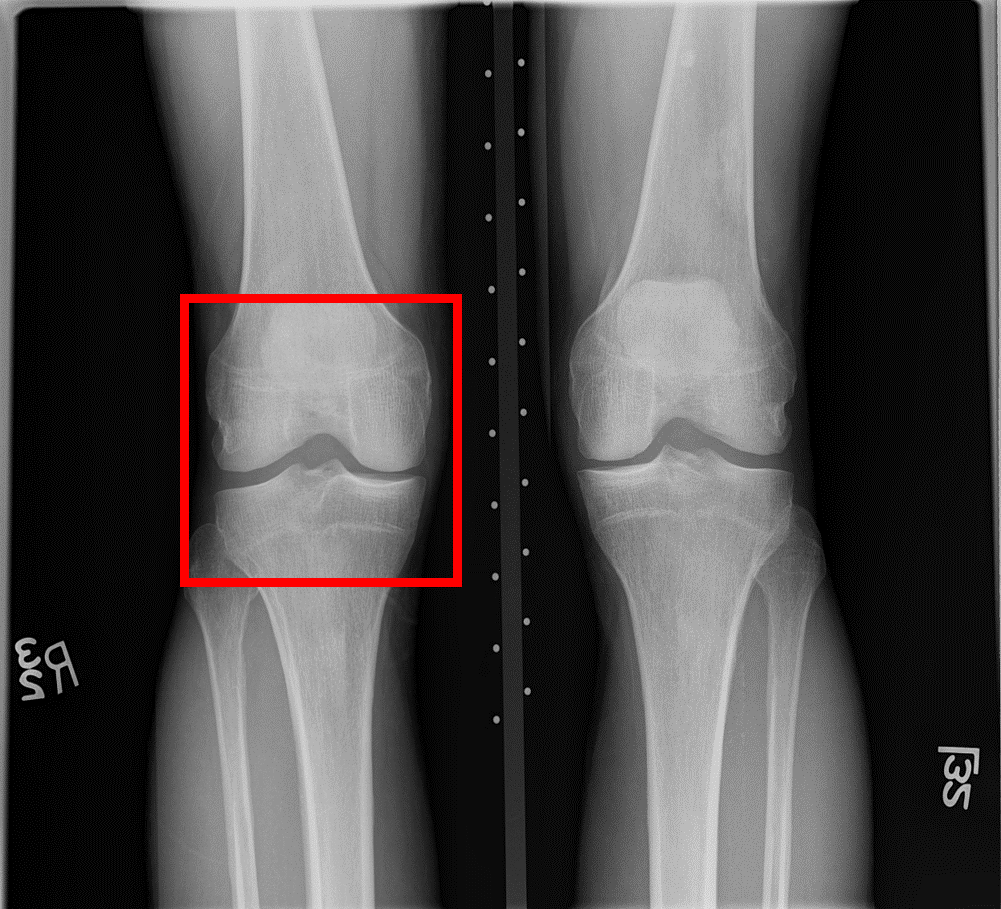
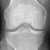
As shown in Fig. 3, the knee joint (Fig. 3) was identified from the plain radiograph (Fig. 3) through the YOLOv2 learning model [29], with images sized of 299 $\times$ 299 $\times$ 1, which were resized to the size of 256$\times$256$\times$1, and image intensity distribution was normalized to [-1, 1].

Figure 3: A standard knee plain radiograph and an identified knee joint highlighted in the red box 3. An identified knee joint 3.

3.2.2 MRI

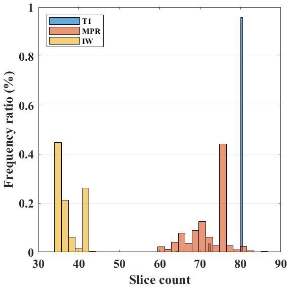
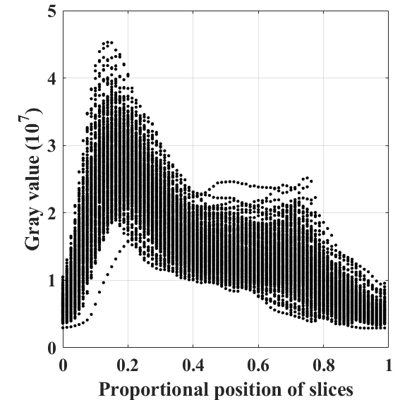
After normalization and standardization, each MRI slice has a size of 256$\times$256$\times$1. To meet the requirements of the pre-trained diffusion model with a channel size of 3, the grayscale images were duplicated three times and then concatenated along the channel dimension. Moreover, the distribution of slice counts was analyzed across three pulse sequences of Intermediate-Weighted (IW), T1-weighted (T1), and Magnetization Prepared Rapid Acquisition Gradient Echo (MPR). As shown in Fig. 4, the slice count for the T1 sequence remains almost consistently fixed at 80, the MPR sequence displays a broader distribution, ranging from 60 to 80 slices, while the IW sequence has the lowest slice counts, between 30 and 40, which suggests that T1 slices are more uniform and contain richer information for model learning. To ensure consistency in our study, we focused exclusively on T1-weighted MRI scans with 80 slices as the original dataset. Fig. 4 illustrates the image intensity distribution within each T1 MRI sequence. As can be seen, grey values rise sharply at first, peaking around the 0.15 proportional slice position. After this peak, the grey values drop steeply by the 0.4 proportional slice position and then gradually taper off, eventually returning to levels similar to those of the initial slices. Based on this and subjective assessment, we extracted slices between the 16$\%$ to 78$\%$ proportional positions (i.e., from the 13th slice to the 63rd one) from each MRI sequence to ensure consistency and avoid low information slices at the beginning and end of the sequence.

Figure 4: Distribution of the number of slices for each type of MRI sequence 4. Grey value distribution at each proportional position of slices within the T1-weighted MRI sequences 4.

After the processing, the slice count was fixed at 50 for the T1-weighted MRI scans as the final experimental dataset. The resulting 4,262 X-ray-MRI pairs were then randomly divided into training and validation sets with a ratio of 7:3.

3.3 Experimental details

The diffusion module utilized pre-trained weights from Zero-123 [30]. The pre-trained KOA classifier $\mathcal{C}$ and encoder $\mathcal{E}_{2}$ were sourced from the [31] and [32], respectively. During the training, a base learning rate of 1e-06 was applied, with a lambda linear scheduler incorporating a warm-up period every 100 steps. The batch size was set to 64, with $T$ configured to 1,000 steps, and an Exponential Moving Average (EMA) [33] of 0.99 was used for the diffusion sampling process. The scale factor of the latent space was set as 0.2. The AdamW optimizer [34] was utilized for training over 5,000 epochs. We implemented our approach using PyTorch v1.8.1 [35] on Nvidia A100 graphics cards with 80 GB of memory.

4 Results and discussion

4.1 Comparisons with State-of-the-Art Methods

In this section, the comparison is divided into two main parts: Qualitative visualization analysis and Quantitative metric-based analysis.

4.1.1 Qualitative visualization analysis

Table 1 provides a comprehensive visual comparison of corresponding pseudo-MRI slices generated by various methods, using X-ray images as input. To facilitate a clear and focused analysis, we selected three representative stages of KOA: G-0, indicating healthy knees; G-2, reflecting early-stage KOA; and G-4, corresponding to late-stage KOA. The compared methods include classic LDM [36], Cola-diff [18], X-diff [37], and our proposed approach. Each row displays the X-ray input on the far left, followed by the real MRI slice and the pseudo-MRI slices generated by the respective methods. To provide a more intuitive illustration of each method’s performance, difference maps generated using a Sobel operator filter are shown beneath each slice, highlighting pixel-wise deviations from the ground truth MRI by detecting edge differences. The visual results consistently show that our model produces pseudo-MRI slices that are closer to the ground truth, with significantly fewer and less pronounced deviations compared to other methods. Specifically, LDM suffers from the lack of constraints provided by the input X-ray. Without this conditional guidance, the model struggles to capture the detailed structural information of the knee joint, leading to great deviations from the ground truth MRI. On the other hand, compared with LDM, although Cola-Diff and X-Diff generate bone structures that are closer to the real MRI in terms of overall shape, they both lack a significant amount of fine details. This limitation prevents them from accurately capturing and reproducing the KOA symptoms. Moreover, it is noteworthy that it is particularly evident as the KOA grade of the input X-ray increases. The progressive narrowing of the knee joint space and the formation of osteophytes are learned and generated more accurately by our model, which demonstrates that our method not only ensures the generation of high-quality pseudo-MRI images but also maintains clinical relevance. However, the model’s predictions in areas outside the skeletal regions are less accurate due to the absence of critical information in X-ray images such as muscle and fat distribution, which will be discussed in Section 4.3.3.

Table 1: Visualization of a representative generated pseudo-MRI slice

X-ray input	MRI Ground Truth∗	LDM	Cola-diff	X-diff	Ours
G-0   Difference
G-2   Difference
G-4   Difference

• Here, to make it more intuitive and convenient, we only display a single slice from each MRI sequence that best represents the complete knee joint.

4.1.2 Quantitative metric-based analysis

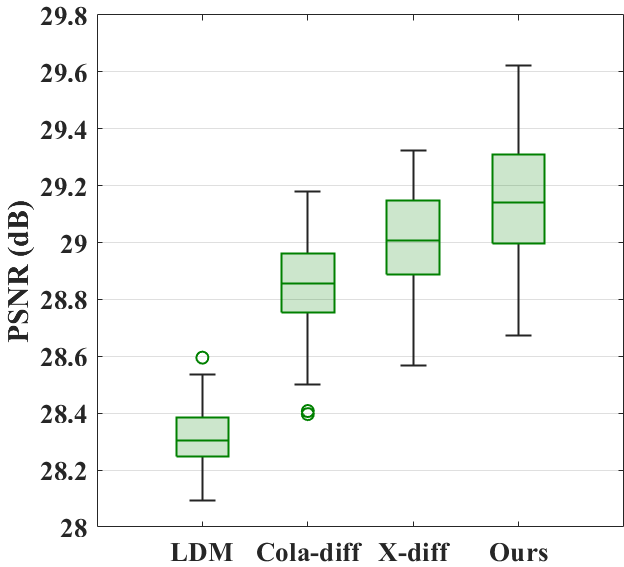
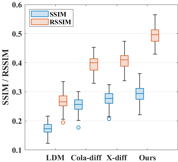
PSNR is a measure used to assess the quality of reconstructed or compressed images compared to their original versions. On the other hand, SSIM is a widely used metric for evaluating the visual similarity between two images considering human visual perception by measuring changes in luminance, contrast, and structural information. However, it does not account for the specific regions of interest (ROI) that are critical in medical imaging. In knee MRI volumes, the most relevant diagnostic information often lies within cartilage, joints, and other areas affected by disease. Therefore, in addition to SSIM, we also adopt a specially designed indicator, the so-called Region-specific Structural Similarity Index (RSSIM), to represent the clinical evaluation of bone morphology. To do so, we utilize the Canny operator with a sigma of 3 to filter and extract bone edges, followed by the application of SSIM. Specifically, we focus on the lower third of the femoral edge to the upper third of the tibial edge to capture ROIs most likely to contain areas of potential pathologies, such as JSN and osteophytes. We compared the performance of the proposed approach with the previously selected methods. Fig. 5 illustrates the statistical distribution of these metrics. As can be seen in Fig. 5, our proposed method has the highest median PSNR, indicating better average image quality, with a median slightly above 29.2 dB. Cola-diff and X-diff also demonstrate a high median around 28.9 dB, with LDM being the lowest, around 28.6 dB. This suggests that, based on the PSNR metric, the image quality performance differences among the four methods are relatively minor. On the other hand, Fig. 5 reveals that while our method achieves the highest median SSIM value, approximately 0.28, the differences between our method, Cola-diff, and X-diff are not substantial, mirroring the trend seen with PSNR. However, our method exhibits a significant advantage under the RSSIM metric. With a median RSSIM value close to 0.5, our approach outperforms the closest competitor, X-diff, which only reaches around 0.42, representing a roughly 20$\%$ improvement, which underscores that our method’s ability to maintain image quality while providing a stronger focus on clinically relevant regions in MRI sequences. Moreover, the above findings emphasize the limitations of traditional image quality metrics as they can not fully capture the distinct differences in Table 1. While these metrics may reflect global image quality in the computer vision domain, they may not be sufficiently sensitive to the specific clinical relevance required in medical imaging.

Figure 5: The box plots visualize the different performance of the evaluated approaches using PSNR 5 and SSIM/RSSIM 5.

4.2 Impact of the number of inference steps

For the inference steps $s$, in addition to adhering to the original depth setting (i.e., $s=S=50$), we also experimented with varying inference steps (i.e., 30, 100, 200, 300, 400, and 500), to explore the impact of increasing the number of inference steps on the quality and accuracy of the generated slices. Fig. 6 shows the adjacent slice correlation coefficients under different inference steps. As can be seen, the red horizontal lines at 0.73 and 0.82 represent the mean adjacent slice correlation coefficients of the pseudo-MRI matching the volume of the original MRI (i.e., $s=S=50$) and that of the original MRI itself, respectively, with the latter serving as the upper benchmark for comparison. At 30 inference steps, the adjacent slice correlation starts at approximately 0.66, reflecting the impact of downsampling, which introduces inconsistencies and reduces the alignment between neighbouring slices. As the number of inference steps increases to 50, where the depth aligns with that of the original MRI volume, the correlation coefficient jumps sharply to around 0.73, suggesting a significant improvement in slice coherence. At 100 steps, the correlation continues to increase modestly. Beyond 100 steps, the improvement becomes more gradual as the number of inference steps increases, with diminishing returns, eventually stabilizing around 0.76 by 500 inference steps.

Figure 6: The adjacent slice correlation coefficients under different inference steps.

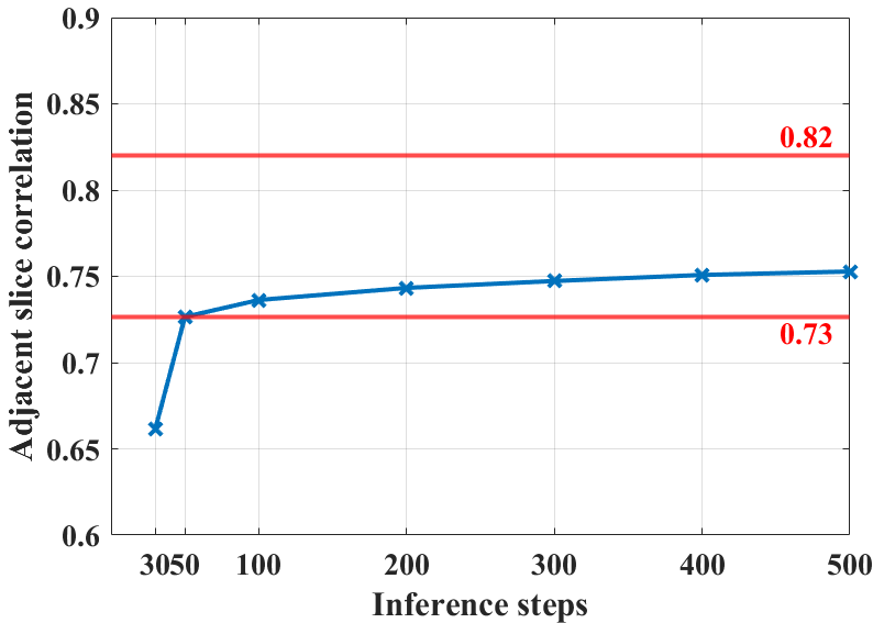
On the other hand, for the sake of clarity and conciseness, we limit our visualization to the interpolation at $s=500$. Table 2 illustrates the synthesized intermediate frames between the original adjacent images (i.e., starting and ending images). Two distinct representative stages were evaluated: The transition from predominantly muscle tissue to the initial appearance of bone, and the shift from cartilage to the developing coronal knee joint. In each of these stages, the synthesized intermediate frames display relatively smooth and continuous transitions between bone and soft tissue structures. Importantly, the model successfully maintains key anatomical details throughout the transition, including the integrity of the bones, cartilage, and joint spaces, which underscores the robustness and effectiveness of these interpolation frames.

Table 2: Visualization of the synthesized intermediate frames

Starting image (real)	$\stackrel{{\scriptstyle\text{Synthesized intermediate frames}}}{{\makebox[284.52756pt]{\rightarrowfill}}}$				Ending image (real)

The above results demonstrate that increasing the number of inference steps $s$ enhances interpolation, showcasing its potential for improving temporal resolution. By generating additional intermediate frames from a smaller set of real frames, interpolation effectively offers more continuous data without lengthening the actual scan duration. On the other hand, despite the improvements observed, the correlation coefficient from the interpolated pseudo-MRI fails to reach the 0.82 benchmark of the original MRI volume, even with the maximum 500 inference steps, which indicates that, while the interpolation process can enhance the consistency between adjacent slices, inherent limitations remain. These limitations arise from the inherent constraints of using X-rays as the sole source of information, which will be discussed in Section 4.3.3.

4.3 Discussion

In this paper, we introduce a novel diffusion-based Xray2MRI model that generates full pseudo-MRI volumes from a single X-ray image, representing one promising initial step toward cost-effective medical imaging solutions. The model leverages conditional inputs from X-rays, combined with target depth, KOA probability distribution, and image intensity distribution modules, to guide the synthesis process and ensure anatomically accurate MRI slice generation. Experimental results show that the generated pseudo-MRI sequences approximate real MRI scans, delivering high image quality while preserving critical clinical relevance. Additionally, by increasing the number of inference steps, the model exhibits effective interpolation, resulting in smoother transitions between slices. Several points are to be discussed.

4.3.1 How it works?

In this approach, we move away from focusing on the distinct imaging principles and techniques of X-ray and MRI. Instead, we only concentrate on the mapping relationship between these two imaging modalities. Much like an extremely experienced senior radiologist who, when viewing an X-ray image, could to some extent mentally infer what the corresponding MRI scans might reveal, which is our proposed AI model’s aim. To this end, for the model’s training, vast amounts of high-quality paired X-ray and MRI have significantly propelled this.

4.3.2 Why use a 2D diffusion model instead of a 3D one directly?

We opted to use a 2D diffusion model, generating individual MRI slices at different target depths during the inference phase, which are then stacked to form a pseudo-3D MRI sequence. By using this method, the model can effectively learn and capture the spatial relationships between the individual slices, allowing it to understand inter-slice dependencies. Additionally, employing a 2D model reduces computational complexity, making both the training and inference processes more efficient compared to handling full 3D data. This approach also enhances the interpretability of the entire process, as it enables a more granular analysis of how each slice contributes to the final 3D reconstruction.

4.3.3 Strengths and limitations

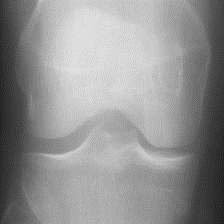
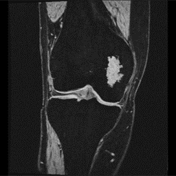
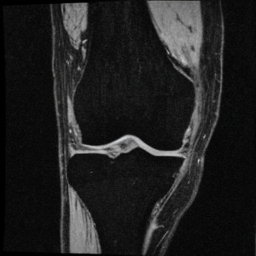
This study has several notable strengths. Firstly, it introduces an innovative method for generating pseudo-MRI images from one single X-ray image, attempting to bridge the gap between these two imaging modalities using advanced AI technology. This approach represents a novel attempt in cases where MRI may not be readily available. Our experiments demonstrate that incorporating supplementary information beyond the X-ray images themselves, such as disease probability distributions, enhances the quality of the generated pseudo-MRI, which underscores the potential of integrating more diverse information sources in the future to produce more accurate pseudo-MRI volumes. Second, the study employs a 2D diffusion model, which not only reduces the computational resources required but also allows for more detailed control over the generated images, leading to a more interpretable and transparent reconstruction process. Finally, the study’s focus on clinically relevant metrics, including both traditional image quality assessments and pathology-specific evaluations, ensures that the generated pseudo-MRI images are not only visually similar to ground truth MRIs but also clinically relevant. This study has several limitations that warrant consideration. First, our model are highly dependent on the availability of large, high-quality paired datasets. The scarcity of such datasets, particularly in certain clinical scenarios or for rare diseases, may limit the generalizability of our approach. Second, although our model is able to approximate MRI features from X-ray inputs, it remains strongly uncertain whether these pseudo-MRI images can be reliably used for clinical diagnosis without the support of additional imaging modalities as the model cannot learn information that is not present in the input X-ray image, which is precisely the value that MRI imaging provides. Such limitation is clearly illustrated in Fig. 7. Finally, the computational resources required for training, despite being reduced by using a 2D model, high-performance hardware is still necessary, which presents a challenge for broader implementation in clinical settings.

(a) X-ray

(b) Real MRI

(c) Generated MRI

Figure 7: The X-ray 7(a) does not provide information about cartilage abnormalities, the generated pseudo-MRI 7(c) thus similarly lacks this detail, whereas such information is presented in the real MRI 7(b).

4.3.4 Future work

More comprehensive information (e.g., BMI, age, gender, disease type and location, etc) could be effectively integrated with X-ray images to further enhance the generation performance. Moreover, to improve the model’s deployability, the use of knowledge distillation could be of interest.

5 Statements

This manuscript was prepared using data from the OAI. The views expressed in it are those of the authors and do not necessarily reflect the opinions of the OAI investigators, the National Institutes of Health (NIH), or the private funding partners.

6 Acknowledgements

The authors gratefully acknowledge the support of the Ralph Schlaeger Research Fellowship under award number 2024A018081 from Massachusetts General Hospital (MGH), Harvard Medical School (HMS).

References

- [1] Richard F Loeser, Steven R Goldring, Carla R Scanzello, and Mary B Goldring. Osteoarthritis: a disease of the joint as an organ. Arthritis and rheumatism, 64(6):1697, 2012.
- [2] Anna Litwic, Mark H. Edwards, Elaine M. Dennison, and Cyrus Cooper. Epidemiology and burden of osteoarthritis. British Medical Bulletin, 105(1):185–199, 01 2013.
- [3] Gurkirpal Singh, Jeffrey D Miller, Fleur H Lee, Dan Pettitt, and Mason W Russell. Prevalence of cardiovascular disease risk factors among us adults with self-reported osteoarthritis: data from the third national health and nutrition examination survey. Population, 7:17, 2002.
- [4] Juan C Mora, Rene Przkora, and Yenisel Cruz-Almeida. Knee osteoarthritis: pathophysiology and current treatment modalities. Journal of pain research, 11:2189, 2018.
- [5] Preeti A Sukerkar and Zoe Doyle. Imaging of osteoarthritis of the knee. Radiologic Clinics, 60(4):605–616, 2022.
- [6] J. H. Kellgren and J. S. Lawrence. Radiological Assessment of Osteo-Arthrosis. Annals of the Rheumatic Diseases, 16(4):494, 1957.
- [7] Felix Eckstein, Flavia Cicuttini, J-P Raynauld, John C Waterton, and Charles Peterfy. Magnetic resonance imaging (mri) of articular cartilage in knee osteoarthritis (oa): morphological assessment. Osteoarthritis and cartilage, 14:46–75, 2006.
- [8] Claudia Lucia Piccolo, Carlo Augusto Mallio, Federica Vaccarino, Rosario Francesco Grasso, and Bruno Beomonte Zobel. Imaging of knee osteoarthritis: a review of multimodal diagnostic approach. Quantitative Imaging in Medicine and Surgery, 13(11):7582, 2023.
- [9] Francisco Reyes-Santias, Carlos García-García, Beatriz Aibar-Guzmán, Ana García-Campos, Octavio Cordova-Arevalo, Margarita Mendoza-Pintos, Sergio Cinza-Sanjurjo, Manuel Portela-Romero, Pilar Mazón-Ramos, and Jose Ramon Gonzalez-Juanatey. Cost analysis of magnetic resonance imaging and computed tomography in cardiology: A case study of a university hospital complex in the euro region. In Healthcare, volume 11, page 2084. MDPI, 2023.
- [10] Robert A Bell. Economics of mri technology. Journal of Magnetic Resonance Imaging, 6(1):10–25, 1996.
- [11] Barbara McLean and Douglas Thompson. Mri and the critical care patient: clinical, operational, and financial challenges. Critical Care Research and Practice, 2023(1):2772181, 2023.
- [12] Jeffrey A Fessler. Model-based image reconstruction for mri. IEEE signal processing magazine, 27(4):81–89, 2010.
- [13] Yoseo Han, Leonard Sunwoo, and Jong Chul Ye. -space deep learning for accelerated mri. IEEE transactions on medical imaging, 39(2):377–386, 2019.
- [14] Michael Lustig, David Donoho, and John M Pauly. Sparse mri: The application of compressed sensing for rapid mr imaging. Magnetic Resonance in Medicine: An Official Journal of the International Society for Magnetic Resonance in Medicine, 58(6):1182–1195, 2007.
- [15] Guang Yang, Simiao Yu, Hao Dong, Greg Slabaugh, Pier Luigi Dragotti, Xujiong Ye, Fangde Liu, Simon Arridge, Jennifer Keegan, Yike Guo, et al. Dagan: deep de-aliasing generative adversarial networks for fast compressed sensing mri reconstruction. IEEE transactions on medical imaging, 37(6):1310–1321, 2017.
- [16] Khosro Bahrami, Feng Shi, Xiaopeng Zong, Hae Won Shin, Hongyu An, and Dinggang Shen. Reconstruction of 7t-like images from 3t mri. IEEE transactions on medical imaging, 35(9):2085–2097, 2016.
- [17] Chenlu Zhan, Yu Lin, Gaoang Wang, Hongwei Wang, and Jian Wu. Medm2g: Unifying medical multi-modal generation via cross-guided diffusion with visual invariant. In Proceedings of the IEEE/CVF Conference on Computer Vision and Pattern Recognition, pages 11502–11512, 2024.
- [18] Lan Jiang, Ye Mao, Xi Chen, Xiangfeng Wang, and Chao Li. Cola-diff: Conditional latent diffusion model for multi-modal mri synthesis. arXiv preprint arXiv:2303.14081, 2023.
- [19] Jonghun Kim and Hyunjin Park. Adaptive latent diffusion model for 3d medical image to image translation: Multi-modal magnetic resonance imaging study. In Proceedings of the IEEE/CVF Winter Conference on Applications of Computer Vision, pages 7604–7613, 2024.
- [20] Robin Rombach, Andreas Blattmann, Dominik Lorenz, Patrick Esser, and Björn Ommer. High-resolution image synthesis with latent diffusion models. In Proceedings of the IEEE/CVF conference on computer vision and pattern recognition, pages 10684–10695, 2022.
- [21] James R Norris. Markov chains. Number 2. Cambridge university press, 1998.
- [22] Olaf Ronneberger, Philipp Fischer, and Thomas Brox. U-net: Convolutional networks for biomedical image segmentation. In Medical image computing and computer-assisted intervention–MICCAI 2015: 18th international conference, Munich, Germany, October 5-9, 2015, proceedings, part III 18, pages 234–241. Springer, 2015.
- [23] Diederik P Kingma. Auto-encoding variational bayes. arXiv preprint arXiv:1312.6114, 2013.
- [24] Yuxin Wu and Kaiming He. Group normalization. In Proceedings of the European conference on computer vision (ECCV), pages 3–19, 2018.
- [25] Prajit Ramachandran, Barret Zoph, and Quoc V Le. Searching for activation functions. arXiv preprint arXiv:1710.05941, 2017.
- [26] A Vaswani. Attention is all you need. Advances in Neural Information Processing Systems, 2017.
- [27] Jiaming Song, Chenlin Meng, and Stefano Ermon. Denoising diffusion implicit models. arXiv preprint arXiv:2010.02502, 2020.
- [28] G. Lester. The Osteoarthritis Initiative: A NIH Public–Private Partnership. HSS Journal: The Musculoskeletal Journal of Hospital for Special Surgery, 8(1):62–63, 2011.
- [29] J. Redmon and A. Farhadi. Yolo9000: better, faster, stronger. In Proceedings of the IEEE conference on computer vision and pattern recognition, pages 7263–7271, 2017.
- [30] Ruoshi Liu, Rundi Wu, Basile Van Hoorick, Pavel Tokmakov, Sergey Zakharov, and Carl Vondrick. Zero-1-to-3: Zero-shot one image to 3d object. In Proceedings of the IEEE/CVF International Conference on Computer Vision (ICCV), pages 9298–9309, October 2023.
- [31] Zhe Wang, Aladine Chetouani, Mohamed Jarraya, Didier Hans, and Rachid Jennane. Transformer with selective shuffled position embedding and key-patch exchange strategy for early detection of knee osteoarthritis. Expert Systems with Applications, 255:124614, 2024.
- [32] Alec Radford, Jong Wook Kim, Chris Hallacy, Aditya Ramesh, Gabriel Goh, Sandhini Agarwal, Girish Sastry, Amanda Askell, Pamela Mishkin, Jack Clark, Gretchen Krueger, and Ilya Sutskever. Learning transferable visual models from natural language supervision. In Marina Meila and Tong Zhang, editors, Proceedings of the 38th International Conference on Machine Learning, volume 139 of Proceedings of Machine Learning Research, pages 8748–8763. PMLR, 18–24 Jul 2021.
- [33] J Stuart Hunter. The exponentially weighted moving average. Journal of quality technology, 18(4):203–210, 1986.
- [34] Ilya Loshchilov and Frank Hutter. Decoupled weight decay regularization, 2019.
- [35] Adam Paszke, Sam Gross, Francisco Massa, Adam Lerer, James Bradbury, Gregory Chanan, Trevor Killeen, Zeming Lin, Natalia Gimelshein, Luca Antiga, Alban Desmaison, Andreas Köpf, Edward Yang, Zach DeVito, Martin Raison, Alykhan Tejani, Sasank Chilamkurthy, Benoit Steiner, Lu Fang, Junjie Bai, and Soumith Chintala. Pytorch: An imperative style, high-performance deep learning library, 2019.
- [36] Robin Rombach, Andreas Blattmann, Dominik Lorenz, Patrick Esser, and Björn Ommer. High-resolution image synthesis with latent diffusion models. In Proceedings of the IEEE/CVF conference on computer vision and pattern recognition, pages 10684–10695, 2022.
- [37] Emmanuelle Bourigault, Abdullah Hamdi, and Amir Jamaludin. X-diffusion: Generating detailed 3d mri volumes from a single image using cross-sectional diffusion models. arXiv preprint arXiv:2404.19604, 2024.