-GLANCE: A Novel Technique to Detect Chromatically and Achromatically Lensed Gravitational Wave Signals
Abstract
Gravitational microlensing occurs when the Schwarzschild radius of the lensing object is smaller or nearly equal to the wavelength of the incoming waves and can produce a chromatic amplitude and phase modulation in the Gravitational Waves (GWs) signal. In contrast, strong gravitational lensing magnifies the incoming gravitational wave in an achromatic way, but can also lead to a constant phase shift. In reality, an observed GW signal can be lensed by both microlensing and strong lensing. To detect and characterize both microlensed and strong lensed GW events together, we have developed a novel method -GLANCE (Micro-Gravitational Lensing Authenticator using Non-modelled Cross-correlation Exploration). In this technique, we calculate the cross-correlation of the residual between different detectors with respect to the best fit and use a generalized template to search for both GW source and lensing parameters. We assign a false alarm rate to each candidate from a statistical viewpoint, depending on how many times the noise cross-correlation matches the strength of the residual cross-correlation of the candidate. We show that for an event with a matched-filtering signal-to-noise ratio (SNR) close to thirty, a residual due to microlensing with an amplitude about of strong lensing magnification will start to show deviation from noise distribution at more than C.I with the LIGO-Virgo-KAGRA sensitivity for the fourth observation run. If the strong lensing or microlensing amplitude is higher (or lower), a lower (or higher) matched-filtering SNR will be required to identify any deviation. This method provides the first technique to detect both strong lensing and micro-lensing without assuming any specific lensing model, and its application on the current and future GW data can identify events with both chromatic and achromatic lensed scenarios.
1 Introduction
Gravitational waves are propagating fluctuations in the spacetime metric caused by the time-varying quadrupole moment of the mass distribution of a system. With the help of Laser Interferometer Gravitational-wave Observatory (LIGO), we have confirmed the existence of gravitational waves on September 14, 2015 [1]. Until the third observational run (O3) in 2021, the LIGO-Virgo-KAGRA detector network (LVK) has more than 90 confirmed detections of GWs [2, 3, 4, 5, 6, 7, 8, 9]. These observations are caused by some of the most catastrophic processes in the universe, such as mergers of compact object binaries. These detections have opened up a plethora of explorable physics regimes, ranging from cosmology (e.g. [10]), compact binary population inferences (e.g. [11]) to probing fundamental physics (e.g. [12]).
Gravitational lensing is the phenomenon where the presence of a massive object dictates the light-like trajectories passing closeby [13, 14, 15, 16, 17]. The massive object bends the path of the incoming gravitational waves, deflecting them from their original trajectories. This causes the waves to interfere, producing amplitude and phase modulation on the outgoing GW waves. Quite analogous to the different regimes of optics with electromagnetic waves, gravitational lensing of GWs can be treated in two different scenarios: (i) Geometric optics: if the Schwarzschild radius () of a massive object (called lens hereafter) is much larger than the wavelength of the emitted gravitational waves (), i.e. , we can consider geometric optics approximation. We observe a system of multiple images with GWs, with frequency-independent magnification and phase-shifts. This is referred to as strong lensing scenario. (ii) Wave optics: if the Schwarzschild radius of the lens is of comparable size or smaller than the wavelength of the GW , interfering signals produce GWs with frequency-dependent amplitude modulation and phase modulation factors. This is referred to as microlensing scenario.
Gravitational lensing provides a unique way to infer the density profile, shape and dimension of the massive lensing objects. While electromagnetic waves lensing happens in the geometric optics regime (due to their short wavelengths compared to the large astrophysical objects in the universe), chances of observing microlensing effects on them are negligibly small. On the other hand, GWs having larger wavelengths (minimum km to maximum km [18]), microlensing of GWs is feasible. Therefore, inference of the shape, size and mass distribution of dark matter structures can be performed by studying the microlensing signatures on GWs. Using lensing of GWs in the observable frequency spectra across all current and future GW detectors, we can probe properties of massive bodies of to mass [19, 20]. Lensing of GWs offers unique probe constraints on the astrophysical population of high redshift compact objects [21, 22], cosmological parameters [23, 24, 25] to study the dark matter distribution [26, 27], testing General Theory of Relativity [28, 29, 30] and to detect intermediate and primordial black holes [31, 32].
With the current LIGO-Virgo-KAGRA(LVK) sensitivities [33, 5, 34], observation of a lensed GW is very rare, having the probability of occurrence of a few parts in a thousand (around 0.1 - 0.6%) [35, 22, 36]. The lensing search by the LVK collaboration on the O3 data led to no significant evidence of any lensing of GWs [37] using existing methods [38, 39, 40, 41, 42, 43]. A follow-up study on the O3 events also did not found any significant evidence of the observation of a lensing event so far [44]. With improved detector sensitivities in the upcoming O5 run and with around GW events, we expect to witness at least one lensed GW.
In the cold dark matter model, we expect large dark matter halos to have smaller subhaloes inside it [45]. So while the halo overall as a lensing object produces strong lensing effects on the GWs, the subhaloes (or any present substructures) can contribute to microlensing modifications [46, 47, 48, 49]. Such scenarios not only allow us to study the properties of the dark matter (DM) halo itself but also let us understand the substructures present within the DM halo. However, the microlensing modifications can be an order of magnitude smaller than the strong lensing [50], therefore making it very hard to be observed. However, with advancements in the GW detectors and with the inclusion of next-generation GW observatories, we expect to be able to distinguish such minuscule modifications on the waveform. Such lensing modifications can impose false bias on estimation of the GW source intrinsic parameters [51].
In this perspective, we have developed -GLANCE, Micro-Gravitational Lensing Authenticator using Non-modelled Cross-correlation Exploration, a technique to detect microlensed gravitational wave signals. The technique essentially relies on the residual cross-correlation among different detectors. Performing cross-correlation on the residuals, helps us understand the common unmodelled features present in the signals as observed in all detectors. To summarize, we perform two distinct parameter estimations on the data: one with the microlensing hypothesis and the other with no microlensing hypothesis. Therefore, in the strong presence of the microlensing in GW signal (reflected by the support of the microlensing parameters in the probability distributions ), we can detect them straightforward. However, if there is no strong support for the microlensing parameters, we shift our focus on the source parameters obtained using the no microlensing hypothesis and construct the best-fit signal. We cross-correlate between the residuals at different detectors and assign a false alarm rate (FAR) associated. If the FAR is less than the threshold FAR, set at per yr, we call the event as an microlensing candidate. On the other side, if there are multiple images of the same GW i.e. in the strong lensing scenario, we apply GLANCE [52] to detect lensed GW signals. We perform cross-correlation on the reconstructed polarizations and its deviation from the noise cross-correlation helps us determine the significance of the event pair being actually lensed.
Recently, there has emerged several search pipelines to detect microlensed GWs. Microlensing, if present in the data, would have some changed characteristics in the spectrogram of the GW. Therefore, deep learning based methods to detect microlensing signatures from the spectrogram has been performed [53]. Microlensing induces a bias to the source parameter estimation. Therefore, to detect microlensing, a joint parameter estimation based technique has also been implemented to obtain the source and microlens parameters together [39]. Also in the presence of a macrolens and microlens substructures inside, strong and microlensing characteristics can be both present on a GW signal. This would enhance the detection of microlensing due to multiple images of the microlensed GW signal; extracting parameters from those multiple signals would allow to better constrain the microlens parameters [54].
In this work, we have presented -GLANCE a novel technique to detect chromatically and achromatically lensed gravitational waves.This work is organised as follows: in section 2, we discuss gravitational lensing of GWs and its strong lensing and microlensing regime. Here, we also motivate about the particular lensing amplification model used in this work. We discuss the salient features of -GLANCE, its strengths and weaknesses in detecting lensed GWs in section 3. In section 4 we discuss the methodology used and the mathematical framework behind the cross-correlation based technique. We apply the technique on simulated GW data in section 5 and show its performance of detecting microlensed signals. In section 6, we present the effect of variation of the source and lens parameters and how that supports us for a confident microlensing detection. To remove the inference biases on the source parameters caused by microlensing, we jointly estimate the source and lens parameters in section 7. The false alarm rate associated with a microlensing detection is calculated in section 8. In section 9, we discuss the possible caveats and the future prospects of -GLANCE in the detection of a microlensed GW.
2 Salient aspects of -GLANCE
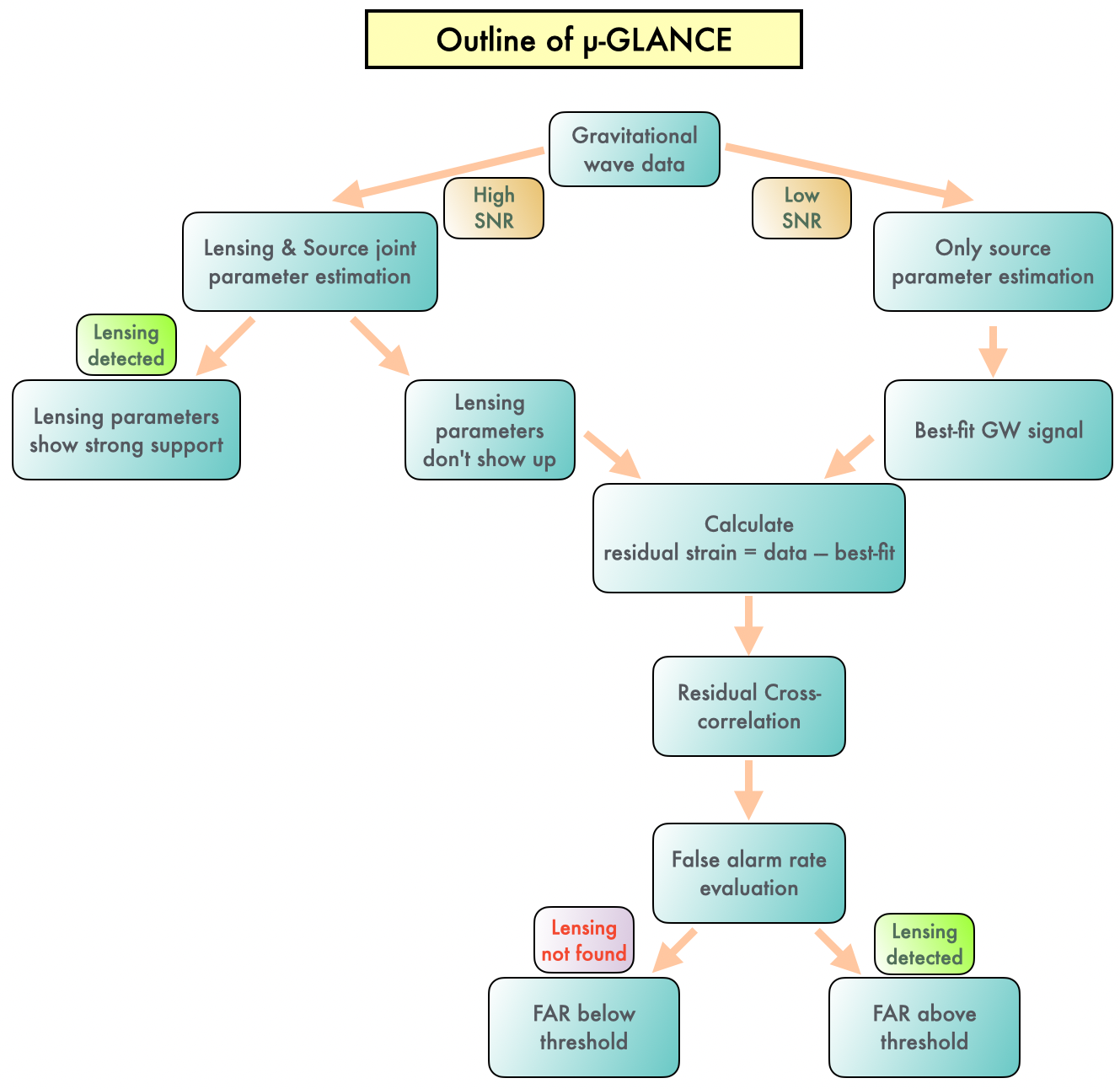
To look for both strong lensing and microlensing signatures present in GW data, we have developed -GLANCE. This method makes both detection and characterization of the lensing signal from the GW data. We show a flowchart describing various parts of -GLANCE in figure 1 and describe some the salient aspects of the method below:
-
•
-GLANCE follows a model independent microlensing search approach towards the data. Using Bayesian parameter estimation technique under a non-lensing hypothesis, the source parameters are constrained to obtain a best-fit strain. The best-fit strain is used to obtain the residual from the data. Cross-correlation is performed on the residuals to observe any non-zero deviation, which can be inferred as a microlensing signature present on the data.
-
•
Lensing modulations can apply bias on the source parameter estimation. Therefore, to remove lensing biases, -GLANCE performs a joint source properties and lens characteristics estimation. We construct a model to capture the microlensing amplification effects caused by an astrophysical object on the GW. Therefore, in contrary to strong lensing searches as in GLANCE [52], the microlensing search is not completely unmodelled. We emphasize that the microlensing parameters show up in the joint distribution when there are microlensing modulation present at significant strength. If the modulations are weakly present, the joint source and lens parameter distribution may not be able to constraint the microlensing parameters correctly and in such cases, we depend on the residual cross-correlation signal to detect any microlensing-like signatures.
Also, we need accurate waveform models to capture all features of the GW. For our current analysis use IMRPhenomXPHM [55] waveform model that incorporates eccentric, precessing black hole binary and calculates the waveform for higher modes starting from 111We have considered the [(2, 2), (2, 1), (3, 3), (3, 2), (4, 4)] and the corresponding negative -modes for the generation of the GW-signal. The inclusion of higher order modes, though marginal in GW data analysis, would have significant impact in the next detectors such as Cosmic Explorer [56] and Einstein Telescope [57]. . In future more accurate waveform model will be required to distinguish between effects arising from waveform mismatch and micro-lensing effects.
3 Basics of Gravitational Lensing: in Microlensing and Strong Lensing Regime
In the presence of matter, the propagation of GW depends on the gravitational potential of object(s) along its trajectory. The equation describing the spatial variation of the GW amplitude is given by [13],
| (3.1) |
where is the 3-dimensional Laplacian operator, is the angular frequency () of the gravitational wave, is the gravitational potential (assumed not to be varying in the scale of the passing time of the GW) of the lens and the GW strain in the frequency domain is given by, where consists of amplitude and phase of the GW and is the associated polarization.
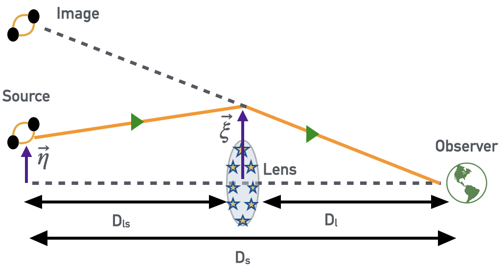
The thin lens approximation assumes that the deflection of the GW caused by the lens happens at the lens plane, a plane passing through the center of the lens at which the lensing object in projected. In figure 2, we have showed a ray diagram schematic for gravitational lensing. Let, be the angular diameter distance 222Angular diameter distance is a distances inferred from the angular size of the sources. See [58] between the observer and the lens, is the angular diameter distance between the observer and the source and is the angular diameter distance between the lens and the source. is the position of the source in the source plane. The source plane origin is located at the intersection the extended straight line joining the the observer to the center of the lens. is the impact parameter of the incoming ray in the lens plane. The origin of the lens plane is located at the center of the lens. We have defined two dimensionless vectors and as following:
| (3.2) |
where sets the characteristic distance scale of the system, called the Einstein radius.
The thin lens approximation is valid when the dimension of the lens is much smaller than the total travelled distance by the GW. The strength of amplification leads to the classification of gravitational lensing as strong lensing or micro-lensing. The amplification factor is defined as . The term at the numerator, is dependent on the relative time delay between the arrival of GWs through different spatial trajectories. This time delay includes the geometric time delay between GWs travelling from different deflected trajectories and the Shapiro time delay, caused by slowing of time at higher spacetime curvature regions. The total time delay is given by [13, 50],
| (3.3) |
where is the redshift of the lens, obtained from its angular diameter distance, be the speed of light in vacuum. The first term provides the geometric time-delay and the second term provides the Shapiro time-delay where provides the gravitational potential of the lens in the lens plane. The third term with is optional, to set the minimum value to zero. In presence of gravitational lensing, GW waves are time-delayed and deflected therefore the addition of GWs in different phases causes interference of lensed GW in the wave-optics limit.
For EM wave passing through an aperture, the amplification factor of the wave at the other side is obtained by using the Kirchhoff integral. A similar expression can be applied for GW lensing. Using the time-delay expression, we can find the amplification factor as,
| (3.4) |
Accounting for the expansion of the universe, the frequencies ’s are all redshifted by a factor of . For a spherically symmetric lens potential, projected on the lens plane, the expression of the amplification factor can be written as,
| (3.5) |
here is the spherical Bessel function of order zero, and is the dimensionless frequency defined as, where is the redshifted mass of the lens, be the frequency of the GW and G is the gravitational constant.
Different lensing regimes can also be described by the dimensionless parameter . When , we are in the wave optics (microlensing) regime, the amplification factor amplitude and its phase are very oscillatory in nature. However, in the limit , we are in the geometric optics (strong lensing) regime. Both and converge to a single value independent of the frequency of the gravitational waves. The amplification factor in the strong lensing regime (for any generic mass or size of lens) becomes,
| (3.6) |
where, the flux-magnification of the j-th image is , and and for minimum, saddle point, maximum of the function. They are known as type-I, type-II and type-III images respectively. Together with these. we can write the lensed wave amplitude in the time-domain is then represented as
| (3.7) |
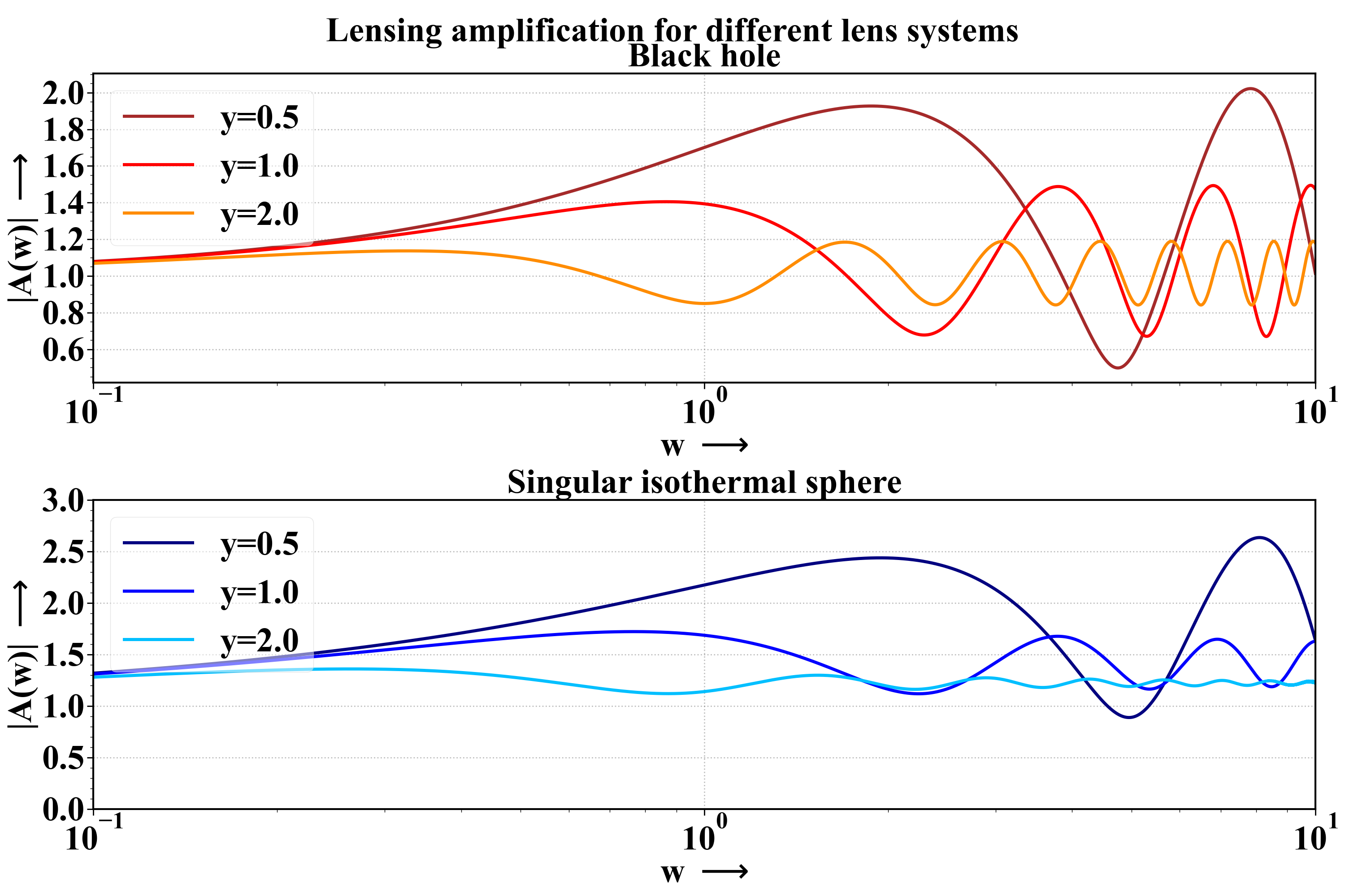
For the black hole lens and singular isothermal sphere profile lens, we have analytic solutions [59]. We plot the solutions as a function of w with y as a parameter in figure 3. However, such analystical solution may not exist for more general lens including assymetric shape and baryonic effects. As a result, for lensing search pipeline to discover signal, it is important for it to capture any general lensing scenario. In a specific lensing model agnostic approach, we have constructed frequency modulated template that captures most (if not all) of the features of microlensing of gravitational waves. The model is described as:
| (3.8) |
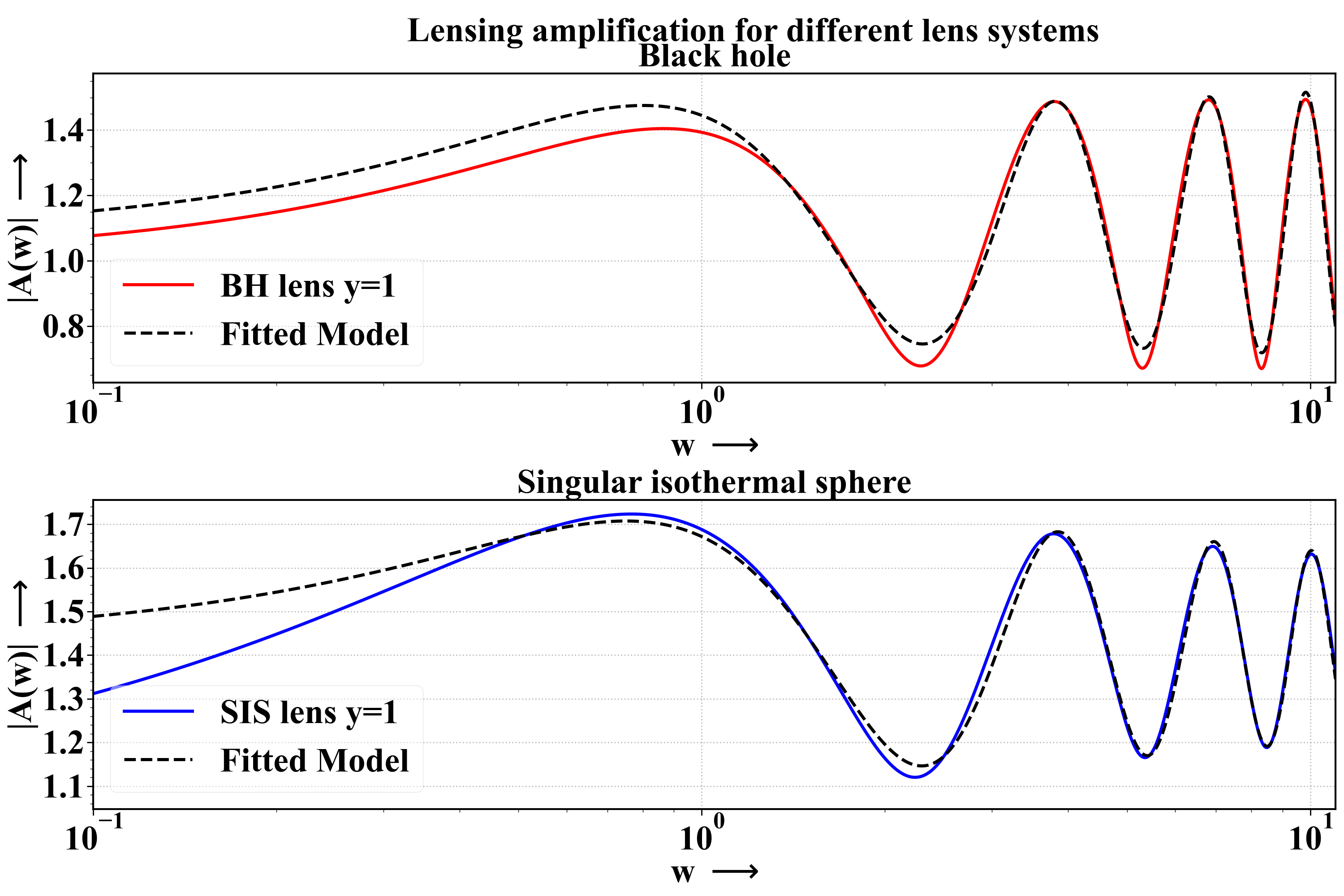
where is microlensing amplitude 333If strong lensing present together with microlensing, it would also contribute to this amplitude, , captures perturbation scale at which the microlensing in the amplification varies, denotes characteristic frequency of the oscillations in amplification, denotes the phase shift due to lensing, and ensures that the amplification slowly converges to as is much greater than . In the later sections, we use this amplification model to understand the different aspects of a microlensing detection and characterization. In figure 4, we have demonstrated the capability to contain all the features in a microlensing amplification for the case with with a BH lens and an SIS lens (With lens of mass at a redshift of ) . The fitting parameters for the black hole amplification profile are and the fitting parameters for the SIS amplification profile are 444Considering no strong lensing , these fitting parameters have been obtained.. We observe that, the amplification model with appropriate fitting parameters can nicely mimic the microlensing amplification555In the current setup, the microlensing model does not capture the phase modulation. But it can be trivially included by a few additional variables to capture the phase modulations, in expense of computational additional time. Thus to demonstrate this technique, we have taken a model with amplitude modulation..
4 Methodology
To obtain the residuals, first we perform a Bayesian parameter estimation technique to constraint the parameters of interest (masses, spins, inclination, distance, RA, Dec, coalescence time, polarization angle) with the unlensed hypothesis. We use the values of the medians of the distributions to obtain a best-fit strain at detector from the data. We subtract this from the data, called , to obtain the residual for the detector , denoted as . Therefore the residual is defined as,
| (4.1) |
here denotes the residual signal and denotes the noise present in the data. We define the cross-correlation between two residual data as from two detectors denoted by ,
| (4.2) |
where is the timescale over which the cross-correlation is performed and be the time-delay between the arrival of the signal (thus the residual) between the detectors. The second expression contains four terms are : , , , respectively, where ‘’ denotes the cross-correlation between them. The final expression is approximated when the cross-correlation timescale () is sufficiently large, comparable to the duration of the signal, the cross-terms do not contribute much.
Therefore, if the absence of any microlensing, the best-fit would be able to capture the GW waveform, making the cross-correlation signal negligible. However, if microlensing present in the GW signal, all its features are not captures by the best-fit signal, therefore it shows up in the cross-correlation. In this analysis, we have ignored waveform systematics and its impact on lensing. The cross-correlation technique can find any non-general relativistic unmodelled signatures present in the signal as well [60].
A similar but distinct detection approach has been taken with strong lensing regime when there are multiple images of a GW signal separated by time delays from seconds to years. We have showed in our previous work GLANCE [52] that, such strongly lensed GW signals can be detected by performing cross-correlation between the reconstructed one-polarization signals of the images using a detector pair at two different times. We defined lensing SNR to quantify how much the cross-correlation signal differs from the noise cross-correlation values. The method demostrates that for type-I and type-II pair (or type-II and type-III pair) of images, the cross-correlation shows up by among the different polarizations, otherwise it shows up in the same polarization. A joint parameter estimation was performed to explore the degeneracies between the source and lens parameters and thus helping in removing the lensing bias. Therefore to look for the strong lensing aspects from the data, we have polarization cross-correlation based technique GLANCE and to look at the microlensing aspects, we have now developed residual cross-correlation based technique -GLANCE.
5 Application of -GLANCE on simulated GW data
As a demonstration of the technique, we generated GW data using a system of binary black holes with masses and at Gpc luminosity distance with inclination angle and dimensionless aligned spins of the primary and the secondary as and respectively. We generate the waveform using the phenomenological model IMRPhenomXPHM [55] and used the analytic noise power spectral density (PSD) model AdVO4T1800545 and AdvVirgo 666See [61] and [62] respectively to generate the noise for the LIGO and Virgo detectors respectively. We choose the amplification factor 777A more generic approach consists of a phase in the cosine term of the amplification factor and estimating that parameter as well, but this form of the amplification bears all the necessary modifications required. In the appendix A, we have showed that the exclusion of the phase does not change any significant results performed in this analysis. as
| (5.1) |
The value of the strong lensing parameter is chosen to be with microlensing perturbation parameter , microlensing oscillation scale parameter Hz and the microlensing convergence parameter . We obtained the best-fit strain without the hypothesis of microlensing present in the data. The data, injected signal and the best-fit (obtained in the frequency domain and then reverted back in time domain) is shown in the figure 5. The contribution of the GW observatory KAGRA is not discussed in this work, since the KAGRA sensitivity is less in comparison to the currently ongoing fourth observation run sensitivity of LIGO and Virgo detectors and therefore inclusion of KAGRA will not make any significant differences in the results.
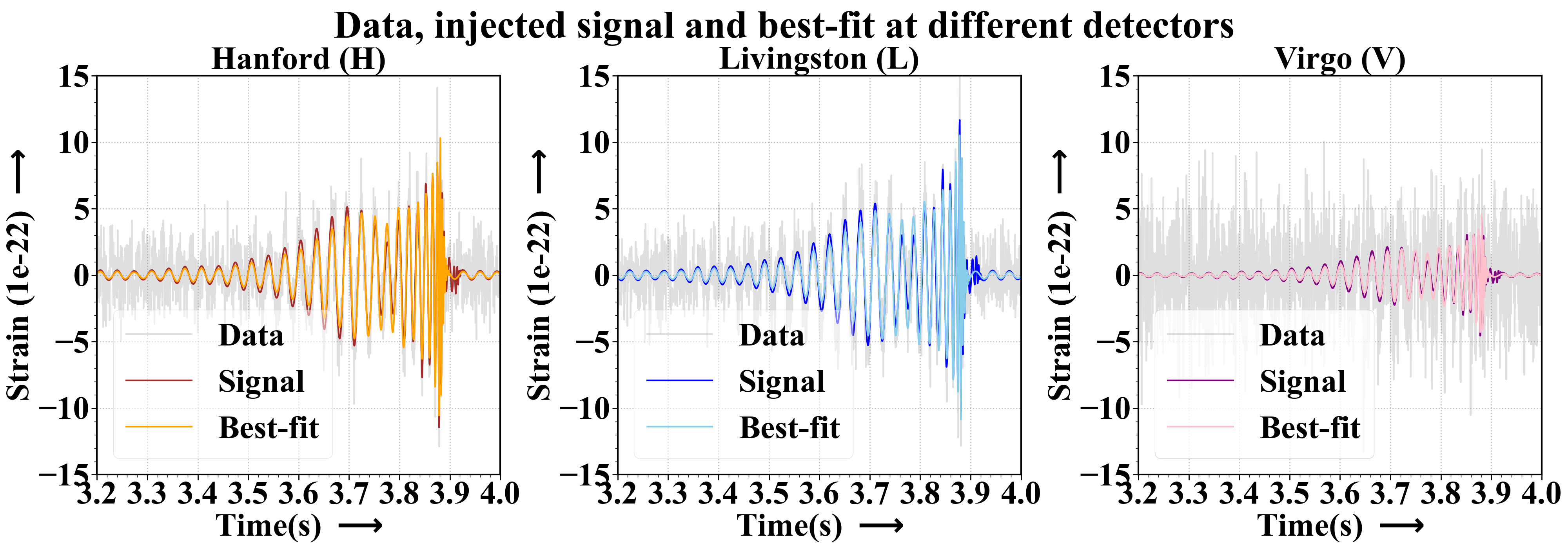
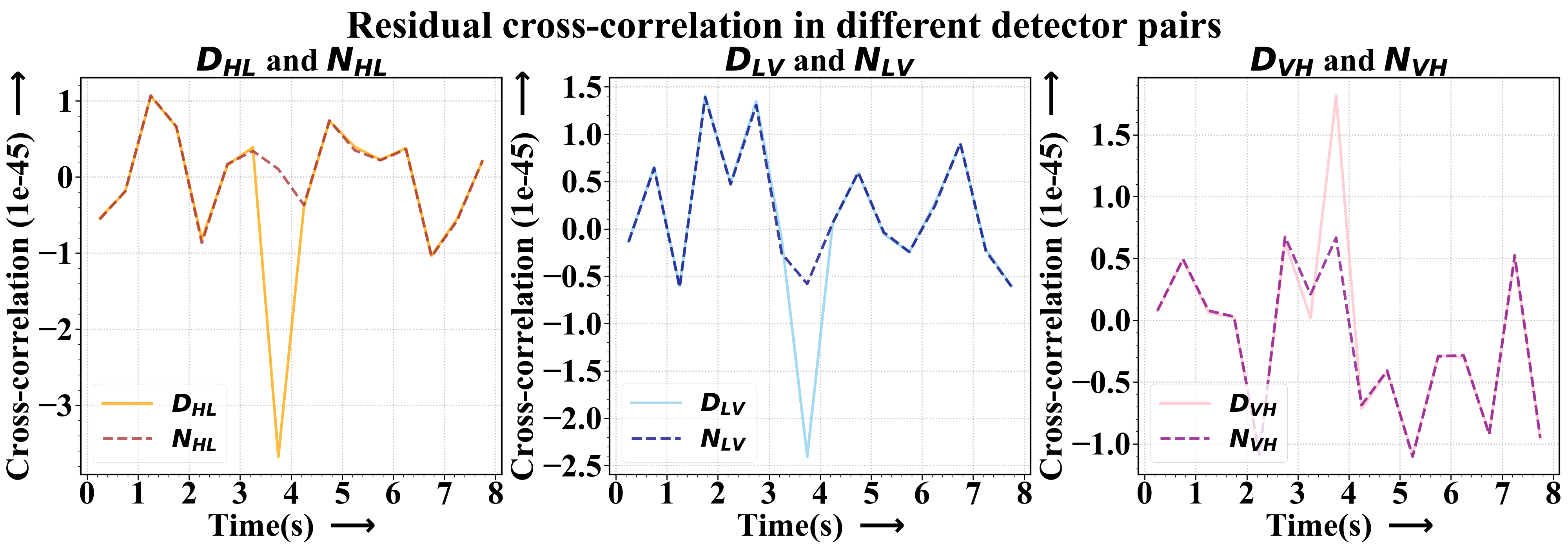
We calculate the residual at each detector by subtracting the best-fit signal from the data. We align the residuals in time by considering the RA and Dec distributions of the GW event in the skymap. We smoothen the data by passing it through a bandpass with lower cut-off and upper cut-off frequencies respectively at Hz and Hz 888The choice of the band is very specific to this example, with lower mass systems, we may need to set up the upper cut-off at higher frequencies. In figure 6, we have shown the residual cross-correlation in the presence of the GW microlensing signal and in the absence of the signal, for pairs formed within LIGO-H, LIGO-L and Virgo-V. The signal is injected close to the fourth second 999The merger happens at the 3.9th second of the signal. in a second long time-series data, that is why we observe a cross-correlation peak at that position. The cross-correlation timescale , since that is the typical duration of the signal. It is noteworthy to mention that, the match-filtering signal to noise ratio (SNR) for the residual drops around 70-80% when compared with the match-filtering SNR obtained from the data.
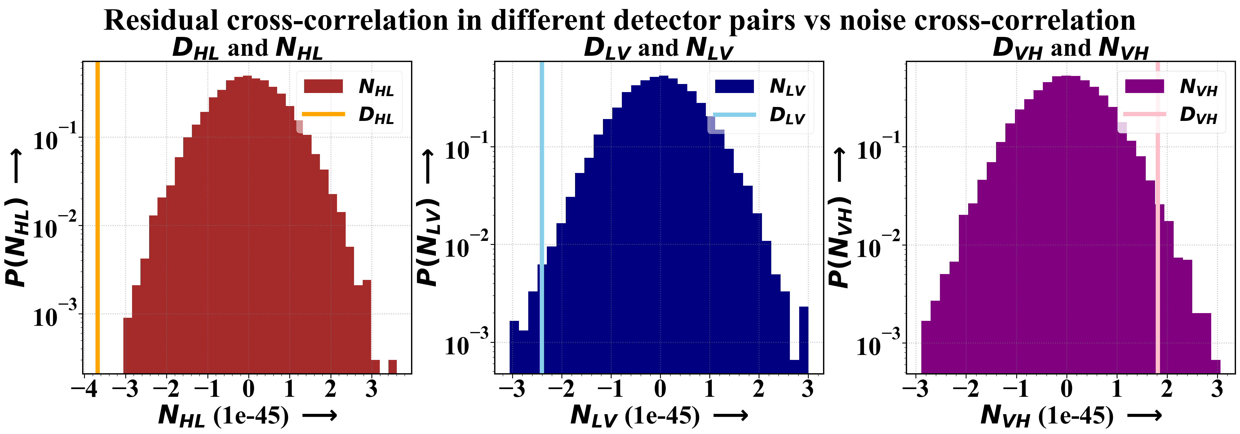
To understand how the residual cross-correlation peak stands out in comparison with the background noise distribution, we have plotted the residual cross-correlation at the timestamp where the signal is present as a line and showed the noise cross-correlation distribution in figure 7. The noise cross-correlation histogram distribution is obtained by generating 1000 noise realizations of second each for all three detectors. Then cross-correlation is performed by taking a pair of noise realization for two different detectors and this is repeated for all the realizations in all possible different detector combinations. These noise cross-correlation values are plotted as the histogram shown in figure 7.
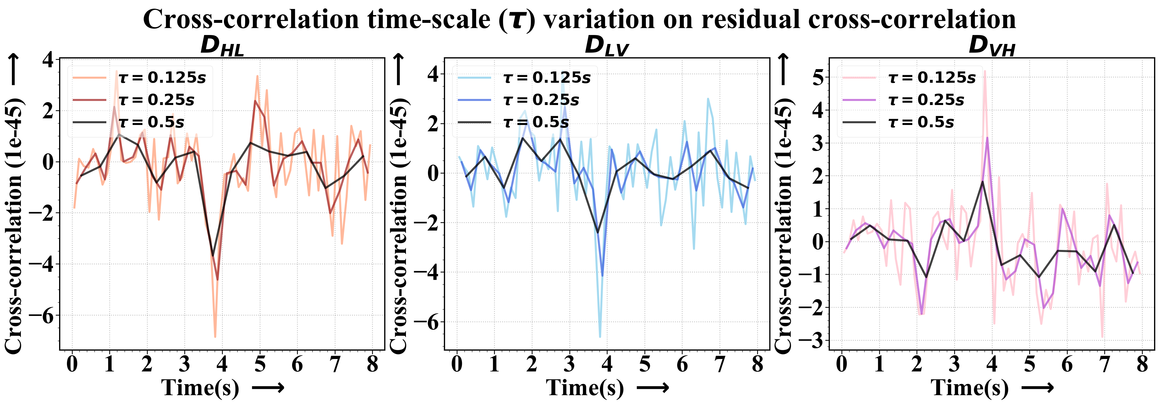
Furthermore, to understand the dependency of the residual cross-correlation signal on the cross-correlation timescale, we have plotted the residual cross-correlation with varying the cross-correlation timescale parameter () in figure 8. It can be clearly observable that as we have increased the timescale , the random noise fluctuation go down faster than the residual cross-correlation signal, making the residual cross-correlation appear more prominent.
6 Cross-correlation Signal Dependency on GW Source and Lens Parameters
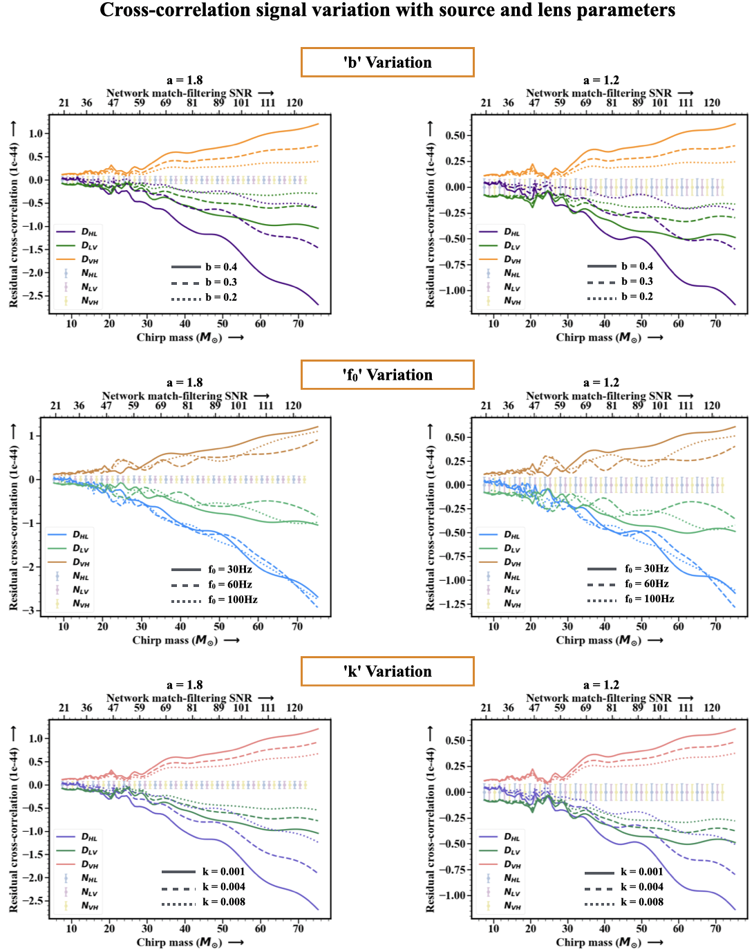
The residual cross-correlation depends on the performance of the unlensed hypothesis parameter estimation to obtain the best-fit GW strain. The better the strain data matches with the best-fit strain is, the smaller is the residual and the residual cross-correlation. However, it is shown in the section 7 that, GW source parameters are well constrained with a model considering no lensing hypothesis even when there is microlensing present. This happens because the source parameters are completely non-degenerate with the lensing template considered in the analysis. Therefore, the residual cross-correlation depends on the strength of the signal, formally given by the match-filtering SNR, that defines how well can we obtain the best-fit. Thus since the microlensing parameters are not captured by the lens parameters in the unlensed hypothesis PE, there exists strongly dependency of the residual cross-correlation on the values of the microlensing parameters. Therefore, to observe how well can we distinguish a lensing modulation, we have checked the variation of the residual cross-correlation with respect to lensing parameters. In figure 9, we have shown the detectability of the residual cross-correlation with respect to the background noise cross-correlation, when no signal is present in the data.
The shaded regions in figure 9, shows the 1- bounds on the noise cross-correlation distribution. The lines show the residual cross-correlation value when the signal consists of microlensing amplification. We varied the chirp mass to increase the strength of the signal. We fixed the value of to 1.2 and 1.8, and then varied the parameters of , and . The luminosity distance of the source is kept fixed at Gpc. The values of the microlensing parameters are chosen in consistency with the numbers obtained in 3 when we fitted the amplification models of BH and SIS with our template in figure 4.
In the first row of the plots, we have varied the value of the microlensing amplitude parameter , keeping and fixed at Hz and respectively. We observe that for , at chirp mass as low as the cross-correlation signal at H-L lies 3- above, however at L-V pair the cross-correlation signal comes above the noise distribution 3- at chirp mass , same for V-H is at around . As the value of b is decreased to a lower value, the minimum chirp mass at which the cross-correlation signal is well distinguishable 101010By ”well distinguishable” we mean that, the residual cross-correlation is at least 3- away from the noise cross-correlation distribution of the BBH shifts towards higher masses. Similarly for with , Hz, we observe that for H-L, L-V, and V-H the cross-correlation signal is distinguishable at , and respectively, which is moved towards higher values as the value of b is decreased.
In the second row of the plots, we have varied the value of the microlensing oscillation parameter , keeping and fixed at and respectively. Unlike the cross-correlation dependency on , we don’t observe a direct observational effect of variation, for any of the detector pairs. For both the cases with and , we observe that the three lines corresponding to Hz, Hz, Hz, the lines are intertwined, not significantly altering the minimum chirp mass at which the cross-correlation signal is distinguishable. We understand that, the value of is more critical to determining microlensing in GW data as compared to .
In the third row of the plots, we have varied the value of the microlensing oscillation converging parameter (as the GW frequencies move towards strong lensing regime), keeping and fixed at and Hz respectively. Quite similar the cross-correlation dependency on , we observe a strong dependency of variation. For the case with , we can distinguish the cross-correlation signal for H-L, L-V, and V-H at , and respectively for the value of . The minimum chirp mass is moved towards the lower end as the value of is decreased. Similarly, with , we can distinguish the cross-correlation signal for H-L, L-V, and V-H at , and respectively for the value of . We understand that the effect of the convergence parameter is similar to the effect of perturbation parameter , therefore making it a very crucial parameter for the detection of microlensing signal.
7 Joint exploration of GW Source Parameters and Lensing Parameters
Lensing can affect the inference of the source properties obtainable from the GW signal through existing parameter estimation techniques. Therefore, a correct approach for inferring source parameters, not just includes the source intrinsic and extrinsic parameters, rather it as well consists of the lens-induced characteristic parameters on the GW signal. We perform Bayesian parameter estimation technique in the frequency domain to jointly explore the parameter space occupied by the source and lens parameters. To showcase the capability of the technique, we choose a simple model for the lensing amplification factor
| (7.1) |
here, we have kept the value of for the simulation set for the purpose of demonstrating the method. The results including is shown in the appendix A. For future analysis of GW data, it can be trivially included in the Bayesian analysis framework. We choose the unlensed signal model given as
| (7.2) |
where denotes the polarization and denotes the detector and and are the antenna patterns associated with the plus and cross polarization. Here , are the masses of the primary and the secondary of the compact binary, is the luminosity distance, is the inclination angle (the angle between the orbital angular momentum and the line of sight). and denote the aligned spin components of the primary and the secondary. The lensed waveform in the frequency domain is the product of the amplification factor and the unlensed signal. Therefore, the lensed signal model is
| (7.3) |
here . Notably, we absorb the effect strong lensing magnification into the luminosity distance of the source to combine an effective distance parameter . Therefore, in the joint source and lens characterization we include source masses, spins, effective luminosity distance and inclination angle along with microlensing modulations.
We formulate the Bayesian parameter estimation using the package BILBY [63], a python-based module extensively used for GW data analysis purposes. We choose uniform priors for the parameters shown in table 1.
| Parameter | Distribution Type | Minimum | Maximum |
|---|---|---|---|
| Uniform | 0 | ||
| Uniform | 0 | 1 | |
| Uniform | 20 | ||
| Uniform | 100 | 7000 | |
| Uniform | 5 | 100 | |
| Uniform | 5 | 100 | |
| inc | Uniform | 0 | |
| Uniform | 0 | 1 | |
| Uniform | 0 | 1 |
The likelihood is a Gaussian and it uses the frequency-domain data and model from all three detectors (in future we can include KAGRA[9] and LIGO-India [64]). The log-likelihood is given by
| (7.4) |
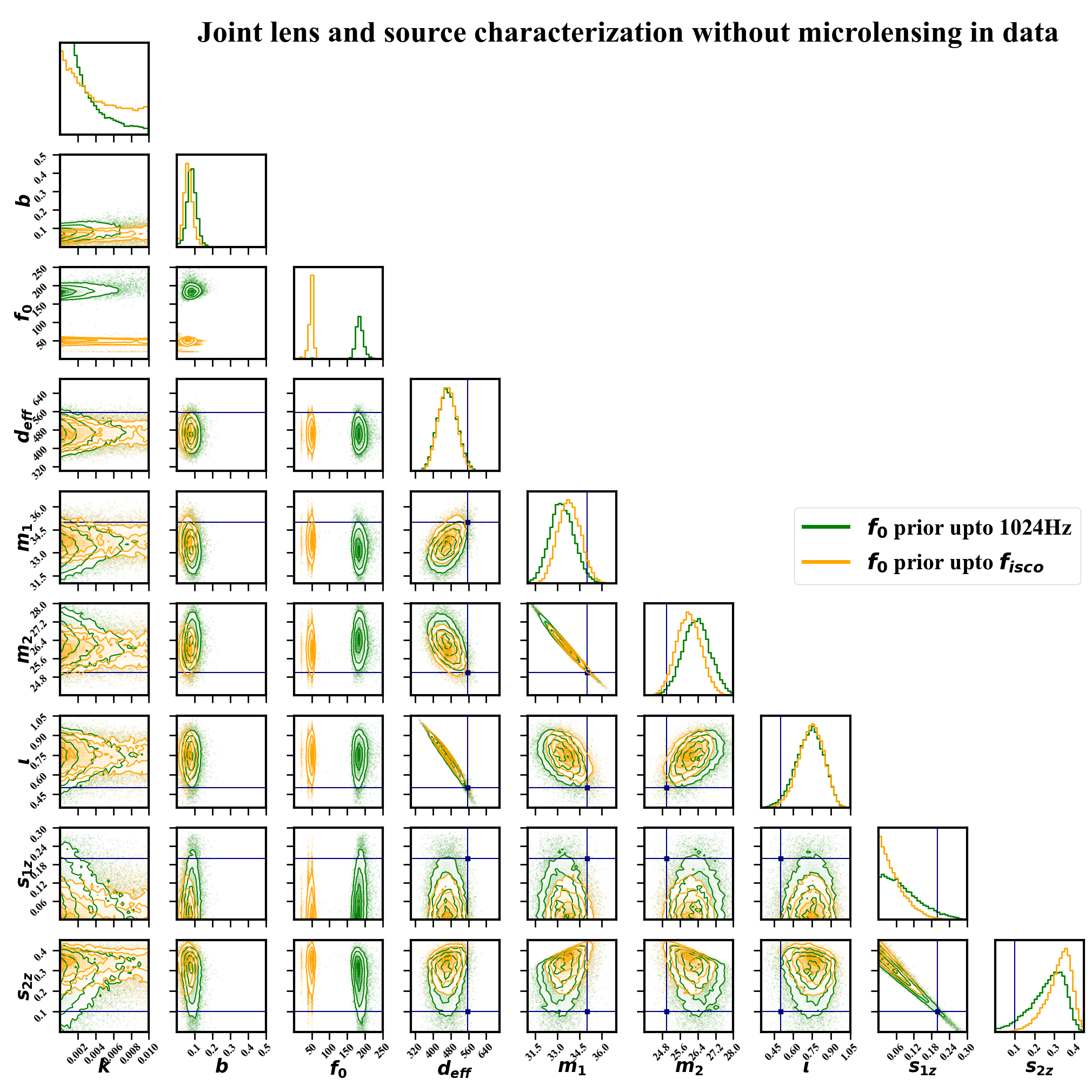
where is the data and is the noise power spectrum density in detector denoted by . We sample the posteriors using nested sampling algorithm DYNESTY [65]. The corner plot consisting of the parameters is shown in figure 10.
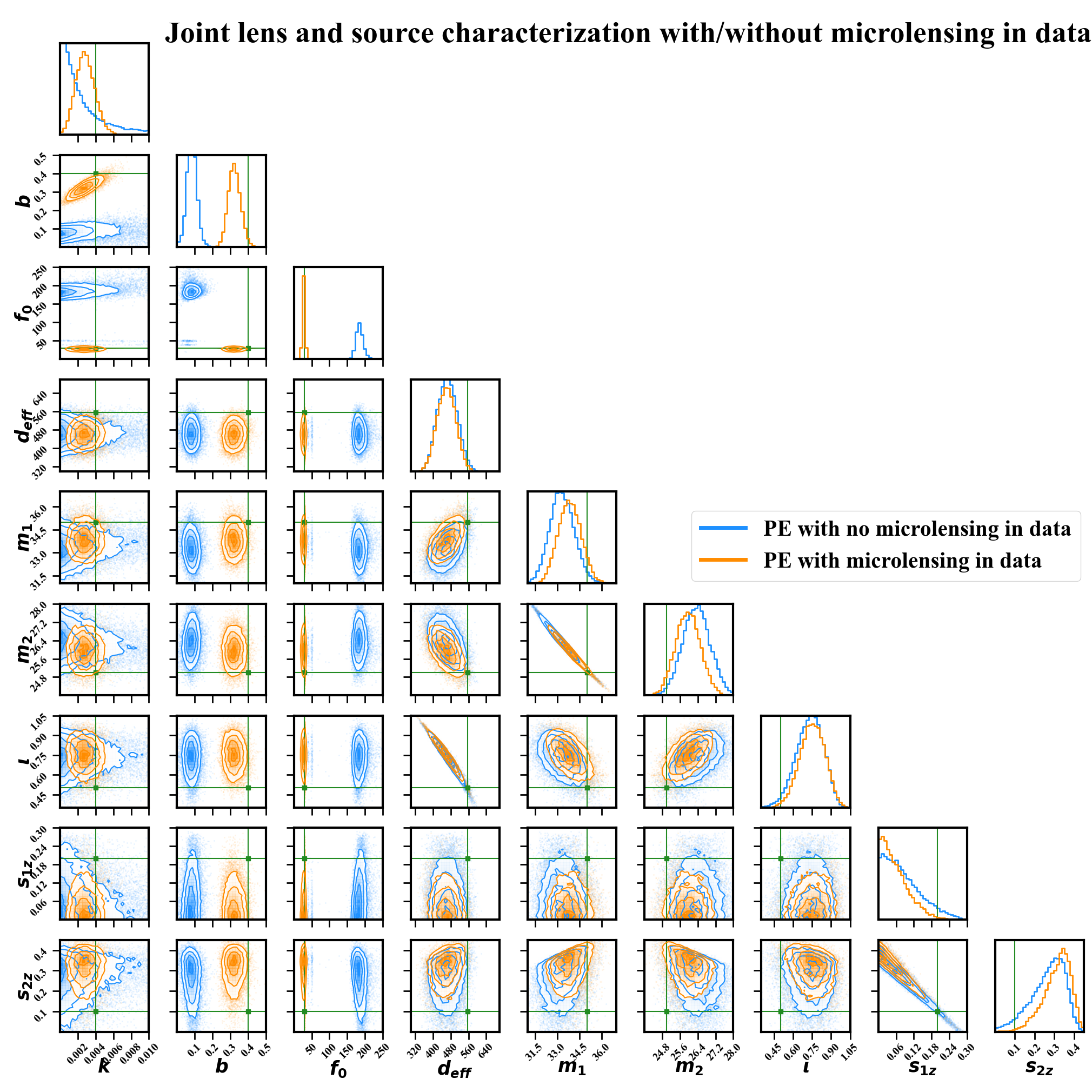
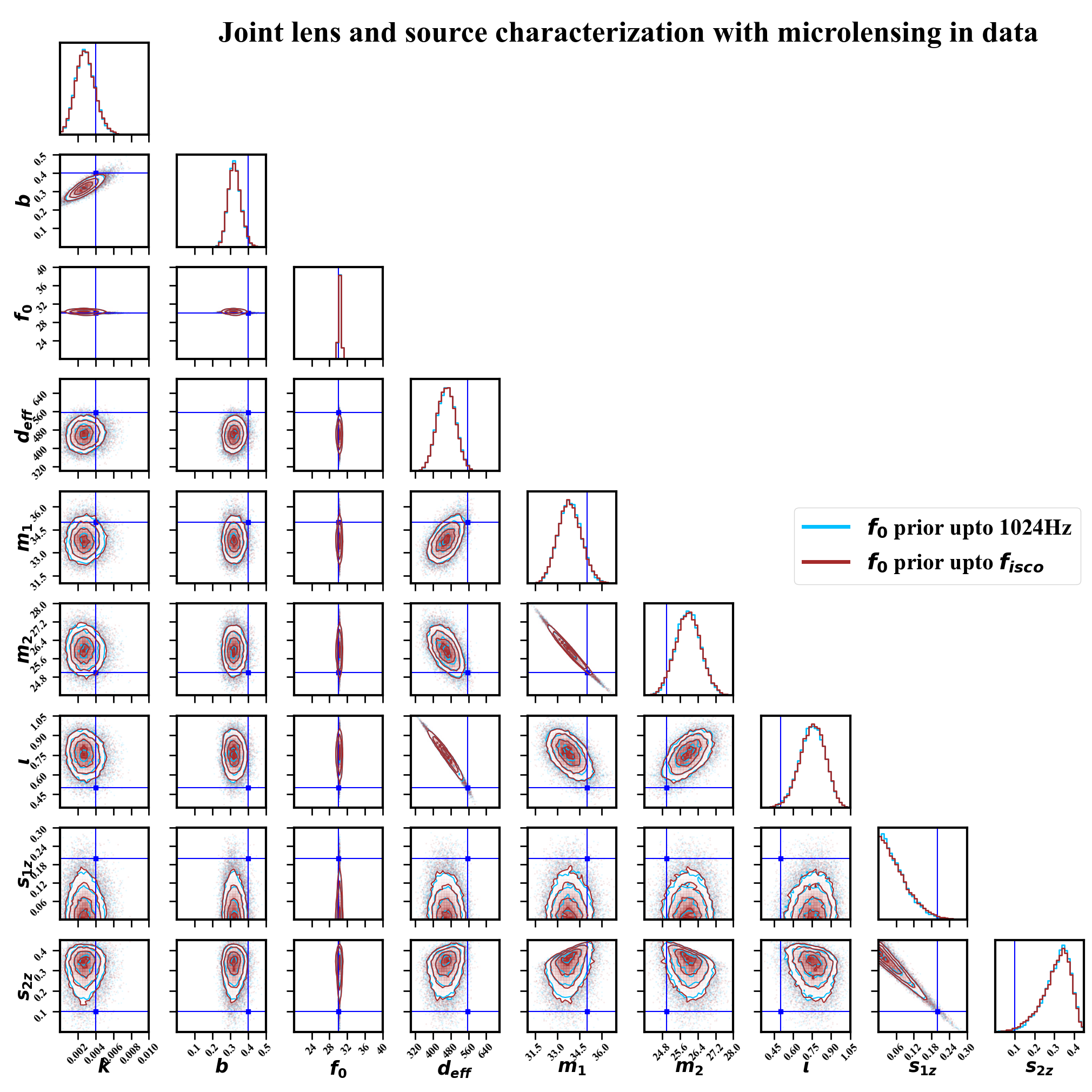
The figure 10 shows the joint parameters of the source and the lens estimated from the data (i) when there is a microlensed GW signal (ii) when there is no microlensed GW signal. The figure has many different aspects to discuss. Firstly, when the microlensing was present in the data, we note that all the parameters are close to well constrained around their injected values, as compared to the other case when the data did not contain a microlensed GW. In the scenario without microlensing, value inclined towards zero, also has a median less than 0.1 and has peaked around 190 Hz which is higher than for these binaries and close to the maximum frequency of emission from this system. The source parameters are well constrained showing almost no deviation in the parameter distributions with microlensing hypothesis. The joint parameter distribution clearly indicates that there is no degeneracy among the source and lens parameters.
On the other hand, we note that the lensing parameters () show no degeneracy with the source parameters (), in particular the oscillation parameter shows no correlation with the source masses , , which control the chirping nature of the signal. We also find that the perturbation parameter is non-degenerate with the aligned spins and which often introduce beating pattern like envelopes on the waveform. This is evident from the fact that, lensing oscillations () and its strength () are coming from the properties of the lens whereas the masses and spins of BBH are its intrinsic properties. Source binary and lensing object involve different timescales of evolution that do not match, therefore the effect of each does not replicate the other, therefore such a correlation between the source and lens parameters is not there. However, we observe that since and for a microlensing event cannot be estimated individually, we combined them in the effective distance parameter , which is well constrained in the range around injected . Finally, we also note that, there is a correlation between and , which was also observed in the figure 9, since the effect of smaller b is equivalent to making b fixed and k larger.
Here we have considered a prior of up to Hz. In appendix B, we have shown that even with a reduced prior of upto , the results of the joint distributions and the best-fit reconstruction has only been affected marginally for the same noise realization. This indicates that use of a large prior on does not adversely impact the results.
8 False Alarm Rate for Microlensing Detection
To understand the significance of a microlensing detection, we have assigned a False Alarm Rate (FAR) with the detections. The false alarms are triggered when there is actually no microlensing signature present in the data, but -GLANCE shows some non-zero cross-correlation signal, caused by the randomness of the noise. We have generated detector noise for Hanford, Livingston, and Virgo with aforementioned noise PSDs for 1 year of observation time. We then performed the cross-correlation between the noise segments of second length of each with a cross-correlation timescale of second. To calculate the FAR (in units of per year), we obtain the residual cross-correlation signal with varying the source and lens parameters and obtain the number of noise cross-correlation points above the certain residual cross-correlation.
In figure 11, we have showed the cumulative distribution function (CDF) of the noise cross-correlation. We have plotted different lines to show the residual cross-correlation strength variation with network match-filtering SNR, by changing the chirp mass of the system. We have also shown the strength of the case we have considered in figure 6, with dashed lines 111111Considering the symmetry of the noise-cross correlation distribution, we have considered the absolute values of the points and plotted its negative. We also did the same for the residual cross-correlation . This was performed to get the probability of a false alarm probability of a residual cross-correlation directly.. We observe that with the system of detector frame BBH masses as at Gpc with lensing parameters , , Hz and , we obtain a false alarm probability of with the residual cross-correlation in H-L pair. Similarly for L-V and V-H pair, we obtain a false alarm probability of few times and . Since the noise distribution is generated with year of simulated noise, the false alarm probabilities directly correspond to the FAR (in yr-1 units) corresponding to the detection of the microlensing search.
From figure 11 we also note that, with increase in the chirp mass and therefore the SNR of the signal, how the residual cross-correlation corresponds to lower FAR. We observe, above network-SNR in H-L and above network-SNR in L-V and V-H, the FAR drops below , making a significant microlensing detection possible. Therefore, the microlensing detection is very probabilistic in high-snr (above 60 network match-filter SNR at least) systems. We suggest to call an event microlensing candidate if the FAR falls below in any of the detector pair. In appendix C, we have showed the effect of different lensing parameters and have estimated the minimum network matched filter SNR required for a low FAR detection ( per year).

9 Conclusion
In this work, we have demonstrated a new technique -GLANCE to search for microlensed GW signals from current detectors. In this method, we performed a model-independent search for microlensing signatures of the GWs by assuming a unlensed hypothesis and obtaining the best-fit GW strain fitting the data. The best-fit is used to calculate the residual signal in each detector. We cross-correlate the aligned residuals and obtain the residual cross-correlation. By comparing with the noise cross-correlation, we obtained a range of source and lensing parameters which would show up against the noise cross-correlation distribution. We also followed a lensing amplification model based approach for the joint exploration of the source and lensing parameters together. Notably, with the chosen simple lensing amplification model, we observe that GW source parameters are not degenerate with the lensing parameters. One important caveat of this technique is that, even if the model-dependent source and lens joint PE technique can work on single-detector events, the model-independent cross-correlation based-search cannot be performed using a single GW detector data.
We would like to emphasize the necessity of using an accurate GW waveform model, that is able to capture all the essential features of compact binary (e.g. eccentricity, precession, higher modes). Otherwise, using inaccurate waveform model, we can observe non-zero residual cross-correlations even when there is no microlensing present in the GW data. To check whether the waveform model is producing residuals even when there is no microlensing, we can put it to a test by checking on a vast different BBH population. If the model is wrong, we may get residuals in many, if not all, of the GW signals and their residual cross-correlations will show up. This is how we can correct waveform model related systematics. However, since the inspiral phase is the longest duration part of the GW signal, and it contributes to most of the signal SNR, any waveform model that can capture the inspiral part well for a coalescing BBH event, can be considered as a good waveform model to search for the lensing signal. However, it is important to point out that though waveform mismodelling may lead to mismodelling of the microlensing parameters, but it is unlikely to impact the search microlensing search pipeline. This is because strain residual from best-fit will capture both waveform systematics and microlensing effects.
Also, in this analysis, we have not incorporated non-stationarity in the strain noise [66, 67, 68]. The non-stationary noise behaviour at one detector is not correlated with the non-stationarity at a different detector, and the duration of a GW signal and the timescale over the which the noise PSD is changing are different. Therefore, we perform cross-correlation on such noise chunks from different detectors at a cross-correlation timescale () much shorter than the variation of the noise-PSD and much longer than a glitch. In this way, we can mitigate the noise fluctuations from generating significant deviations from zero residual cross-correlation 121212We also apply bandpass filter to remove very low frequencies where noise-fluctuation is very high and very high frequencies where the jitters are very faster than the signal oscillations .
The current analytic lensing model we use in this analysis, captures most of the features present in microlensing amplification in general. However, we do not claim universality to this amplification template. It shows to be working nicely with the two test cases we used in 3. It may fail badly for some lens models present in the universe. However this would not impact the residual cross-correlation since, obtaining the best-fit strain at a detector and from there obtaining the residual and finally performing the residual cross-correlation – each step is done in a model independent approach. Therefore, when the amplification template fails, although hinders the joint parameter space exploration side, does not affect the microlensing detection side, which is a completely data-driven model-agnostic approach for a robust technique to detect microlensed GWs. However, we have not associated any of the microlensing parameters , , , to physical space parameters in the lens system, like the offset parameter , the mass of the lens or its density profile . This will be performed in a future work.
With the gradual advancement of the ground-based GW detector sensitivities, and the inclusion of the next-generation like Cosmic Explorer (CE) [56], Einstein Telescope (ET) [57] or Laser Interferometer Space Antenna (LISA) [69], the microlensing signatures in the cross-correlation is expected to be predominant over noise cross-correlation distribution. This will allow microlensed GW signals to be detected at an unprecedented precision. The microlensing amplification can lead to inferring the intrinsic properties of the lensing object. Therefore, under the wave-optics regime, the microlensing aspects would allow us to probe the dark matter haloes and subhaloes, which are otherwise invisible to the electromagnetic signal. In this regard, -GLANCE will play a pivotal role in both the detection and precise characterization of microlensing signatures, significantly enhancing our ability to identify and analyze these phenomena with greater efficiency.
Acknowledgments
The authors are thankful to Sourabh Magare for reviewing the manuscript during the LSC Publications and Presentations procedure and providing useful comments. The authors express their gratitude to the ⟨data|theory⟩ Universe-Lab group-members for useful suggestions. This work is part of the ⟨data|theory⟩ Universe-Lab, supported by TIFR and the Department of Atomic Energy, Government of India. The authors express gratitude to the computer cluster of ⟨data|theory⟩ Universe-Lab for computing resources used in this analysis. We thank the LIGO-Virgo-KAGRA Scientific Collaboration for providing noise curves. LIGO, funded by the U.S. National Science Foundation (NSF), and Virgo, supported by the French CNRS, Italian INFN, and Dutch Nikhef, along with contributions from Polish and Hungarian institutes. The research leverages data and software from the Gravitational Wave Open Science Center, a service provided by LIGO Laboratory, the LIGO Scientific Collaboration, Virgo Collaboration, and KAGRA. Advanced LIGO’s construction and operation receive support from STFC of the UK, Max-Planck Society (MPS), and the State of Niedersachsen/Germany, with additional backing from the Australian Research Council. Virgo, affiliated with the European Gravitational Observatory (EGO), secures funding through contributions from various European institutions. Meanwhile, KAGRA’s construction and operation are funded by MEXT, JSPS, NRF, MSIT, AS, and MoST. This material is based upon work supported by NSF’s LIGO Laboratory which is a major facility fully funded by the National Science Foundation. We acknowledge the use of the following python packages in this work: NUMPY [70], SCIPY [71], MATPLOTLIB [72], GWSIM [73], ASTROPY[74], PYCBC [75], GWPY [76], LALSUITE [77], EMCEE [78] and CORNER [79], BILBY [80].
Notes:
The data files and result plots shown in this work will be available on the ⟨data|theory⟩ Universe-Lab GITHUB page. Its usage in a research work must be done with proper consent from the authors.
References
- [1] LIGO Scientific, Virgo collaboration, Observation of Gravitational Waves from a Binary Black Hole Merger, Phys. Rev. Lett. 116 (2016) 061102 [1602.03837].
- [2] LIGO Scientific, Virgo collaboration, GWTC-1: A Gravitational-Wave Transient Catalog of Compact Binary Mergers Observed by LIGO and Virgo during the First and Second Observing Runs, Phys. Rev. X 9 (2019) 031040 [1811.12907].
- [3] LIGO Scientific, Virgo collaboration, GWTC-2: Compact Binary Coalescences Observed by LIGO and Virgo During the First Half of the Third Observing Run, Phys. Rev. X 11 (2021) 021053 [2010.14527].
- [4] KAGRA, VIRGO, LIGO Scientific collaboration, GWTC-3: Compact Binary Coalescences Observed by LIGO and Virgo during the Second Part of the Third Observing Run, Phys. Rev. X 13 (2023) 041039 [2111.03606].
- [5] KAGRA, LIGO Scientific, Virgo collaboration, Prospects for observing and localizing gravitational-wave transients with Advanced LIGO, Advanced Virgo and KAGRA, Living Rev. Rel. 19 (2016) 1 [1304.0670].
- [6] VIRGO collaboration, Advanced Virgo: a second-generation interferometric gravitational wave detector, Class. Quant. Grav. 32 (2015) 024001 [1408.3978].
- [7] LIGO Scientific collaboration, Advanced LIGO, Class. Quant. Grav. 32 (2015) 074001 [1411.4547].
- [8] A. Buikema, C. Cahillane, G. Mansell, C. Blair, R. Abbott, C. Adams et al., Sensitivity and performance of the advanced ligo detectors in the third observing run, Physical Review D 102 (2020) .
- [9] KAGRA collaboration, Overview of KAGRA: Detector design and construction history, PTEP 2021 (2021) 05A101 [2005.05574].
- [10] LIGO Scientific, Virgo, KAGRA collaboration, Constraints on the Cosmic Expansion History from GWTC–3, Astrophys. J. 949 (2023) 76 [2111.03604].
- [11] KAGRA, VIRGO, LIGO Scientific collaboration, Population of Merging Compact Binaries Inferred Using Gravitational Waves through GWTC-3, Phys. Rev. X 13 (2023) 011048 [2111.03634].
- [12] LIGO Scientific, VIRGO, KAGRA collaboration, Tests of General Relativity with GWTC-3, 2112.06861.
- [13] P. Schneider, J. Ehlers and E.E. Falco, Gravitational Lenses, Springer (1992), 10.1007/978-3-662-03758-4.
- [14] Y. Wang, A. Stebbins and E.L. Turner, Gravitational lensing of gravitational waves from merging neutron star binaries, Phys. Rev. Lett. 77 (1996) 2875.
- [15] T.T. Nakamura, Gravitational lensing of gravitational waves from inspiraling binaries by a point mass lens, Phys. Rev. Lett. 80 (1998) 1138.
- [16] M. Bartelmann, Gravitational lensing, Classical and Quantum Gravity 27 (2010) 233001.
- [17] L. Dai, T. Venumadhav and K. Sigurdson, Effect of lensing magnification on the apparent distribution of black hole mergers, Phys. Rev. D 95 (2017) 044011.
- [18] M. Bailes et al., Gravitational-wave physics and astronomy in the 2020s and 2030s, Nature Rev. Phys. 3 (2021) 344.
- [19] J. Wambsganss, Gravitational lensing, in Encyclopedia of Mathematical Physics, J.-P. Françoise, G.L. Naber and T.S. Tsun, eds., (Oxford), pp. 567–575, Academic Press (2006), DOI.
- [20] D. Bayer, L.V.E. Koopmans, J.P. McKean, S. Vegetti, T. Treu, C.D. Fassnacht et al., Probing sub-galactic mass structure with the power spectrum of surface-brightness anomalies in high-resolution observations of galaxy-galaxy strong gravitational lenses – I. Power-spectrum measurement and feasibility study, Mon. Not. Roy. Astron. Soc. 523 (2023) 1326 [2302.00480].
- [21] S. Mukherjee, T. Broadhurst, J.M. Diego, J. Silk and G.F. Smoot, Inferring the lensing rate of LIGO-Virgo sources from the stochastic gravitational wave background, Mon. Not. Roy. Astron. Soc. 501 (2021) 2451 [2006.03064].
- [22] S. Mukherjee, T. Broadhurst, J.M. Diego, J. Silk and G.F. Smoot, Impact of astrophysical binary coalescence time-scales on the rate of lensed gravitational wave events, Monthly Notices of the Royal Astronomical Society 506 (2021) 3751 [https://academic.oup.com/mnras/article-pdf/506/3/3751/39456853/stab1980.pdf].
- [23] M. Sereno, P. Jetzer, A. Sesana and M. Volonteri, Cosmography with strong lensing of LISA gravitational wave sources, Mon. Not. Roy. Astron. Soc. 415 (2011) 2773 [1104.1977].
- [24] A. Balaudo, A. Garoffolo, M. Martinelli, S. Mukherjee and A. Silvestri, Prospects of testing late-time cosmology with weak lensing of gravitational waves and galaxy surveys, JCAP 06 (2023) 050 [2210.06398].
- [25] S. Jana, S.J. Kapadia, T. Venumadhav and P. Ajith, Cosmography Using Strongly Lensed Gravitational Waves from Binary Black Holes, Phys. Rev. Lett. 130 (2023) 261401 [2211.12212].
- [26] R. Massey, T. Kitching and J. Richard, The dark matter of gravitational lensing, Rept. Prog. Phys. 73 (2010) 086901 [1001.1739].
- [27] S. Basak, A. Ganguly, K. Haris, S. Kapadia, A.K. Mehta and P. Ajith, Constraints on Compact Dark Matter from Gravitational Wave Microlensing, Astrophys. J. 926 (2022) L28 [2109.06456].
- [28] X.-L. Fan, K. Liao, M. Biesiada, A. Piorkowska-Kurpas and Z.-H. Zhu, Speed of Gravitational Waves from Strongly Lensed Gravitational Waves and Electromagnetic Signals, Phys. Rev. Lett. 118 (2017) 091102 [1612.04095].
- [29] S. Mukherjee, B.D. Wandelt and J. Silk, Probing the theory of gravity with gravitational lensing of gravitational waves and galaxy surveys, Mon. Not. Roy. Astron. Soc. 494 (2020) 1956 [1908.08951].
- [30] S. Mukherjee, B.D. Wandelt and J. Silk, Multimessenger tests of gravity with weakly lensed gravitational waves, Phys. Rev. D 101 (2020) 103509 [1908.08950].
- [31] K.-H. Lai, O.A. Hannuksela, A. Herrera-Martín, J.M. Diego, T. Broadhurst and T.G.F. Li, Discovering intermediate-mass black hole lenses through gravitational wave lensing, Phys. Rev. D 98 (2018) 083005.
- [32] M. Oguri and R. Takahashi, Probing Dark Low-mass Halos and Primordial Black Holes with Frequency-dependent Gravitational Lensing Dispersions of Gravitational Waves, Astrophys. J. 901 (2020) 58 [2007.01936].
- [33] B.P. Abbott et al., Sensitivity of the Advanced LIGO detectors at the beginning of gravitational wave astronomy, Phys. Rev. D 93 (2016) 112004 [1604.00439].
- [34] aLIGO collaboration, Sensitivity and performance of the Advanced LIGO detectors in the third observing run, Phys. Rev. D 102 (2020) 062003 [2008.01301].
- [35] S.-S. Li, S. Mao, Y. Zhao and Y. Lu, Gravitational lensing of gravitational waves: a statistical perspective, Monthly Notices of the Royal Astronomical Society 476 (2018) 2220.
- [36] J. Diego, T. Broadhurst and G. Smoot, Evidence for lensing of gravitational waves from ligo-virgo data, Physical Review D 104 (2021) .
- [37] The LIGO Scientific Collaboration, the Virgo Collaboration, the KAGRA Collaboration, R. Abbott, H. Abe, F. Acernese et al., Search for gravitational-lensing signatures in the full third observing run of the LIGO-Virgo network, arXiv e-prints (2023) arXiv:2304.08393 [2304.08393].
- [38] J. Janquart, O.A. Hannuksela, K. Haris and C. Van Den Broeck, A fast and precise methodology to search for and analyse strongly lensed gravitational-wave events, Monthly Notices of the Royal Astronomical Society 506 (2021) 5430 [https://academic.oup.com/mnras/article-pdf/506/4/5430/39656596/stab1991.pdf].
- [39] M. Wright and M. Hendry, Gravelamps: Gravitational Wave Lensing Mass Profile Model Selection, 2112.07012.
- [40] R.K.L. Lo and I. Magaña Hernandez, Bayesian statistical framework for identifying strongly lensed gravitational-wave signals, Phys. Rev. D 107 (2023) 123015.
- [41] O.A. Hannuksela, K. Haris, K.K.Y. Ng, S. Kumar, A.K. Mehta, D. Keitel et al., Search for gravitational lensing signatures in LIGO-Virgo binary black hole events, Astrophys. J. Lett. 874 (2019) L2 [1901.02674].
- [42] L. Dai, B. Zackay, T. Venumadhav, J. Roulet and M. Zaldarriaga, Search for Lensed Gravitational Waves Including Morse Phase Information: An Intriguing Candidate in O2, 2007.12709.
- [43] L.P. Singer, D.A. Goldstein and J.S. Bloom, The Two LIGO/Virgo Binary Black Hole Mergers on 2019 August 28 Were Not Strongly Lensed, 1910.03601.
- [44] J. Janquart, M. Wright, S. Goyal, J.C.L. Chan and A. Ganguly, Follow-up analyses to the O3 LIGO–Virgo–KAGRA lensing searches, Monthly Notices of the Royal Astronomical Society 526 (2023) 3832 [https://academic.oup.com/mnras/article-pdf/526/3/3832/52108394/stad2909.pdf].
- [45] J. Zavala and C.S. Frenk, Dark matter haloes and subhaloes, Galaxies 7 (2019) 81 [1907.11775].
- [46] M. Fairbairn, J. Urrutia and V. Vaskonen, Microlensing of gravitational waves by dark matter structures, JCAP 07 (2023) 007 [2210.13436].
- [47] J.M. Diego, O.A. Hannuksela, P.L. Kelly, T. Broadhurst, K. Kim, T.G.F. Li et al., Observational signatures of microlensing in gravitational waves at LIGO/Virgo frequencies, Astron. Astrophys. 627 (2019) A130 [1903.04513].
- [48] J.M. Diego, Constraining the abundance of primordial black holes with gravitational lensing of gravitational waves at ligo frequencies, Phys. Rev. D 101 (2020) 123512.
- [49] A.K. Meena, Gravitational lensing of gravitational waves: prospects for probing intermediate-mass black holes in galaxy lenses with global minima image, Mon. Not. Roy. Astron. Soc. 532 (2024) 3568 [2305.02880].
- [50] R. Takahashi and T. Nakamura, Wave effects in gravitational lensing of gravitational waves from chirping binaries, Astrophys. J. 595 (2003) 1039 [astro-ph/0305055].
- [51] A. Mishra, A.K. Meena, A. More and S. Bose, Exploring the impact of microlensing on gravitational wave signals: Biases, population characteristics, and prospects for detection, Mon. Not. Roy. Astron. Soc. 531 (2024) 764 [2306.11479].
- [52] A. Chakraborty and S. Mukherjee, GLANCE – Gravitational Lensing Authenticator using Non-modelled Cross-correlation Exploration of Gravitational Wave Signals, Mon. Not. Roy. Astron. Soc. 532 (2024) 4842 [2403.03982].
- [53] K. Kim, J. Lee, O.A. Hannuksela and T.G.F. Li, Deep Learning–based Search for Microlensing Signature from Binary Black Hole Events in GWTC-1 and -2, Astrophys. J. 938 (2022) 157 [2206.08234].
- [54] E. Seo, O.A. Hannuksela and T.G.F. Li, Improving Detection of Gravitational-wave Microlensing Using Repeated Signals Induced by Strong Lensing, Astrophys. J. 932 (2022) 50 [2110.03308].
- [55] G. Pratten et al., Computationally efficient models for the dominant and subdominant harmonic modes of precessing binary black holes, Phys. Rev. D 103 (2021) 104056 [2004.06503].
- [56] M. Evans et al., A Horizon Study for Cosmic Explorer: Science, Observatories, and Community, 2109.09882.
- [57] M. Maggiore et al., Science Case for the Einstein Telescope, JCAP 03 (2020) 050 [1912.02622].
- [58] D.W. Hogg, Distance measures in cosmology, astro-ph/9905116.
- [59] G. Tambalo, M. Zumalacárregui, L. Dai and M.H.-Y. Cheung, Lensing of gravitational waves: Efficient wave-optics methods and validation with symmetric lenses, Phys. Rev. D 108 (2023) 043527.
- [60] G. Dideron, S. Mukherjee and L. Lehner, New framework to study unmodeled physics from gravitational wave data, Phys. Rev. D 107 (2023) 104023 [2209.14321].
- [61] L. Barsotti, S. Gras, M.Evans and P. Fritschel, The updated Advanced LIGO design curve, 2018.
- [62] A. Manzotti and A. Dietz, Prospects for early localization of gravitational-wave signals from compact binary coalescences with advanced detectors, 1202.4031.
- [63] G. Ashton et al., BILBY: A user-friendly Bayesian inference library for gravitational-wave astronomy, Astrophys. J. Suppl. 241 (2019) 27 [1811.02042].
- [64] B. Iyer, T. Souradeep, C. Unnikrishnan, S. Dhurandhar, S. Raja and A. Sengupta, LIGO India - Proposal of the Consortium for Indian Initiative in Gravitational-wave Observations (IndIGO), 2011.
- [65] J.S. Speagle, dynesty: a dynamic nested sampling package for estimating bayesian posteriors and evidences, Monthly Notices of the Royal Astronomical Society 493 (2020) 3132–3158.
- [66] LIGO Scientific, VIRGO collaboration, Identification of long-duration noise transients in LIGO and Virgo, Class. Quant. Grav. 28 (2011) 235008 [1108.1521].
- [67] S. Mozzon, L.K. Nuttall, A. Lundgren, T. Dent, S. Kumar and A.H. Nitz, Dynamic normalization for compact binary coalescence searches in non-stationary noise, Classical and Quantum Gravity 37 (2020) 215014.
- [68] S. Mozzon, G. Ashton, L.K. Nuttall and A.R. Williamson, Does nonstationary noise in LIGO and Virgo affect the estimation of H0?, Phys. Rev. D 106 (2022) 043504 [2110.11731].
- [69] LISA collaboration, Astrophysics with the Laser Interferometer Space Antenna, Living Rev. Rel. 26 (2023) 2 [2203.06016].
- [70] C.R. Harris, K.J. Millman, S.J. van der Walt, R. Gommers, P. Virtanen, D. Cournapeau et al., Array programming with NumPy, Nature 585 (2020) 357.
- [71] P. Virtanen, R. Gommers, T.E. Oliphant, M. Haberland, T. Reddy, D. Cournapeau et al., SciPy 1.0: Fundamental Algorithms for Scientific Computing in Python, Nature Methods 17 (2020) 261.
- [72] J.D. Hunter, Matplotlib: A 2d graphics environment, Computing in Science & Engineering 9 (2007) 90.
- [73] C. Karathanasis, B. Revenu, S. Mukherjee and F. Stachurski, GWSim: Python package for creating mock GW samples for different astrophysical populations and cosmological models of binary black holes, Astron. Astrophys. 677 (2023) A124 [2210.05724].
- [74] T.A. Collaboration, A.M. Price-Whelan, P.L. Lim, N. Earl, N. Starkman, L. Bradley et al., The astropy project: Sustaining and growing a community-oriented open-source project and the latest major release (v5.0) of the core package, The Astrophysical Journal 935 (2022) 167.
- [75] A. Nitz, I. Harry, D. Brown, C.M. Biwer, J. Willis, T.D. Canton et al., gwastro/pycbc: v2.3.3 release of pycbc, Jan., 2024. 10.5281/zenodo.10473621.
- [76] D.M. Macleod, J.S. Areeda, S.B. Coughlin, T.J. Massinger and A.L. Urban, GWpy: A Python package for gravitational-wave astrophysics, SoftwareX 13 (2021) 100657.
- [77] LIGO Scientific Collaboration, Virgo Collaboration and KAGRA Collaboration, “LVK Algorithm Library - LALSuite.” Free software (GPL), 2018. 10.7935/GT1W-FZ16.
- [78] D. Foreman-Mackey, D.W. Hogg, D. Lang and J. Goodman, emcee: The mcmc hammer, Publications of the Astronomical Society of the Pacific 125 (2013) 306–312.
- [79] D. Foreman-Mackey, corner.py: Scatterplot matrices in python, The Journal of Open Source Software 1 (2016) 24.
- [80] G. Ashton, M. Hübner, P.D. Lasky, C. Talbot, K. Ackley, S. Biscoveanu et al., Bilby: A user-friendly bayesian inference library for gravitational-wave astronomy, The Astrophysical Journal Supplement Series 241 (2019) 27.
- [81] J.D. Peter Fritschel, Kevin Kuns et al., Report from the LSC Post-O5 Study Group, 2024.
- [82] E.D. Hall et al., Gravitational-wave physics with Cosmic Explorer: Limits to low-frequency sensitivity, Phys. Rev. D 103 (2021) 122004 [2012.03608].
- [83] M. Punturo et al., The Einstein Telescope: A third-generation gravitational wave observatory, Class. Quant. Grav. 27 (2010) 194002.
Appendix A Appendix: Inclusion of amplification template phase term in the source and lens joint PE
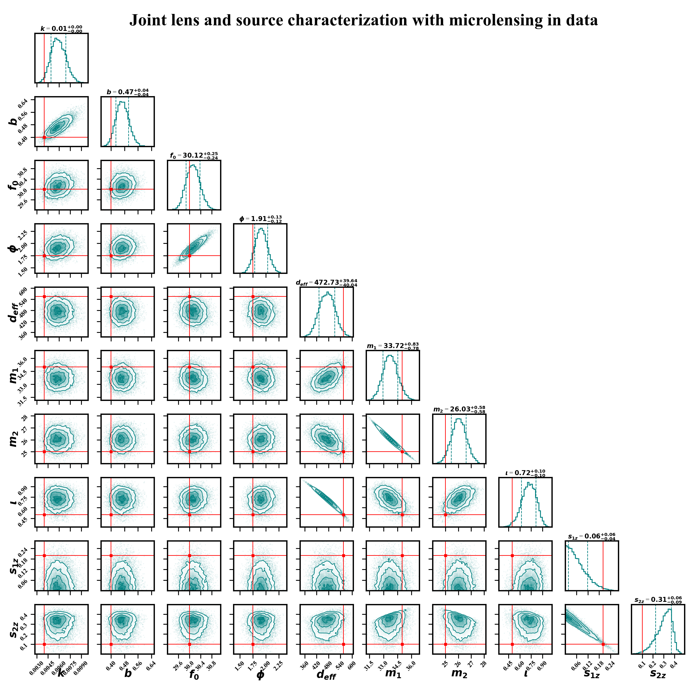
Here we have included the phase of the amplification in the joint parameter exploration. The figure 12 shows that, with the inclusion of the phase of the amplification, which was not considered in the analysis, for obvious reasons, does not affect the rest of the source and lens parameters. This shows that the phase term has no correlation with any of the other source and lens parameters and our results without the phase are absolutely fine to consider.
Appendix B Appendix: Effect of Different Choices of Priors on Parameter Estimation
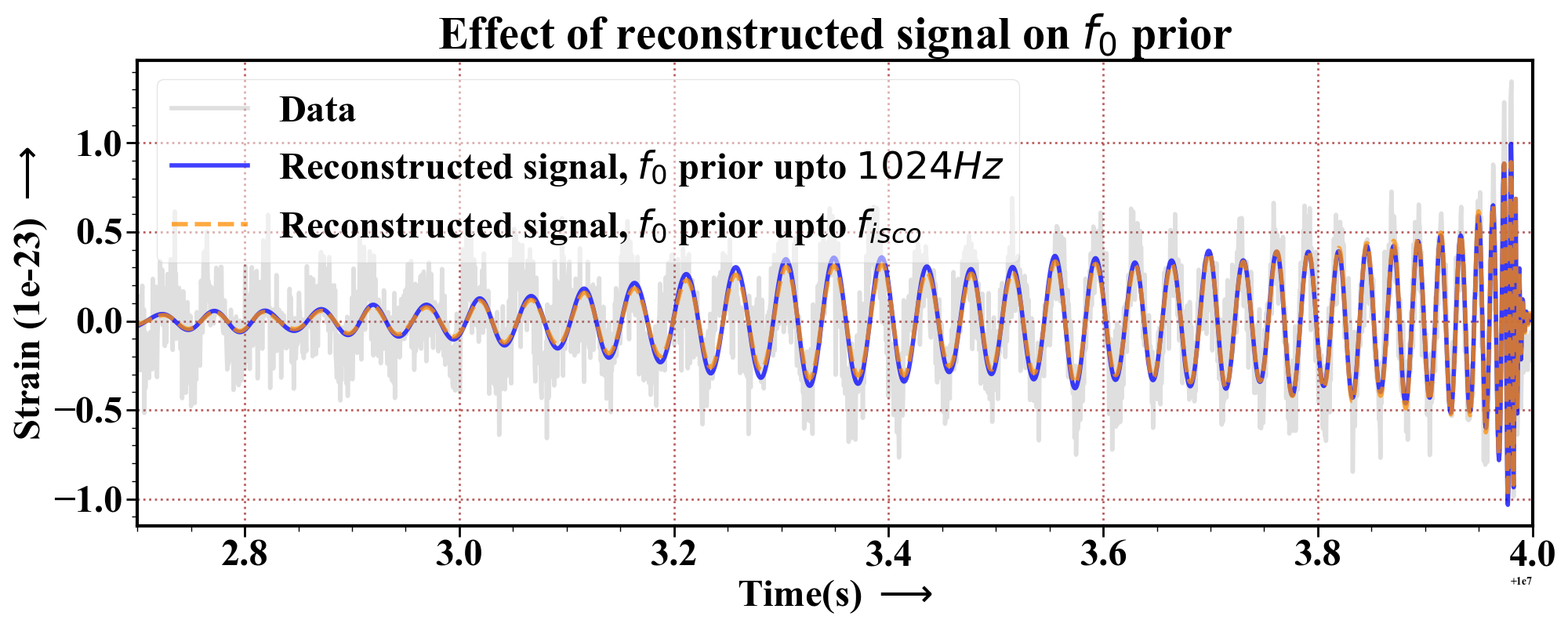
To understand whether we have effects on the posteriors caused by the choice of the priors, especially for the case when there was no microlensing injected in the data. We study the effect of the choice of the parameter , for which we have two different priors: (i) Hz and (ii) Hz, where is the innermost stable circular orbit frequency of the binary black holes and is the final frequency of the the frequency-series data.
We have plotted the frequency-domain data and the waveform model is constructed with the medians of the posteriors. To compare with we have shown in figure 13 that, we do not observe any direct effect of the choice of prior, since the medians of the microlensing perturbation parameter was very close to being zero. The medians of for both the cases with prior up to Hz and are 0.0877 and 0.0764 respectively, therefore not showing any microlensing features prominently. We also obtained the joint distribution of the microlensing and source parameters when the signal was not microlensed, with those two different priors. The comparison of the choice of such different prior choices is shown in figure 14. Similarly, we obtained the joint distribution of the microlensing and source parameters when the signal was actually microlensed, with those two different priors. The comparison of the choice of such different prior choices is shown in figure 15.
Appendix C Appendix: False Alarm Rates Depending on Source and Lens Parameters
In figure 11, we obtained the FAR for a particular combination of lens parameters and varied the strength of the signal by varying the chirp mass of the compact binary. Here we present a few more combinations of the lensing parameters, it shows the confidence at which we are going to detect them.
We fixed the oscillation parameter since from figure 9 we observed that the residual cross-correlation signal has no direct dependency on the value of . Therefore, we only varied , , and to show at what FAR we can detect microlensing events.
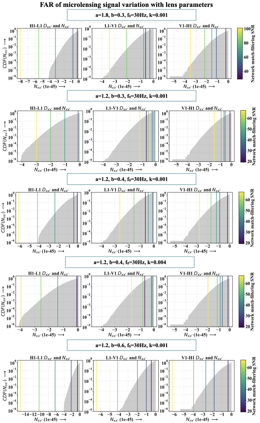
In figure 16, we varied the network matched-filtering SNR and observe the dependency of FAR of the microlensing detection, depending on the values of , , and . We show on the first pane for at and , it shows that close to network SNR of 70, we can have a FAR on at least one detector pair below . For the case considering , and , the minimum network SNR is still at around 65 to detect a microlensing signal. This is because the effect of the strong lensing magnification has been absorbed in the luminosity distance while performing the parameter estimation for the best-fit. For the case with , and , we observe that the minimum network SNR is close to 45, where for the same and values, with , it is moved back to 55. Finally, with , and , the minimum network SNR required is about 35.
From this study, we can conclude that microlensing is hard to detect with current generation GW detectors unless the SNR of the source is very high. With the inclusion of more detectors and better detector sensitivites such as LIGO-India [64], A# [81], CE[82] or ET[83] observatories, detection of microlensing events will be more feasible. The availability of more detectors and better detector sensitivity will help in obtaining cross-correlation signals between more pairs of detectors (, where is the number of detectors) and will also help in reducing the FAR. As a result, will make it feasible for robust detection of the microlensing signatures from GW signals.