Are intrinsic decoherence models physical theories?

Abstract

Intrinsic decoherence models (IDMs) have been proposed in order to solve the measurement problem in quantum mechanics. In this work, we assess the status of two of these models as physical theories by establishing the ultimate bounds on the estimability of their parameters. Our results show that dephasing and dissipative IDMs are amenable to falsification and should be considered physical theories worth of experimental study.

I Introduction

Quantum mechanics is a self-consistent theory that has consistently aligned with experimental results. Its only issues are rooted in conceptual difficulties. These difficulties present when we try to account for macroscopic objects and their interactions with microscopic ones and are strictly related to the occurrence of linear superpositions of macroscopically distinguishable states of a macroscopic system [1, 2].

Decoherence of macroscopic systems is often attributed to their interaction with the external environment. Indeed, when a system is coupled with another and we only look at the state of the first system neglecting the second one, it loses coherence and evolves into a statistical mixture, eventually resembling a classical system. Since macroscopic systems are always coupled, unlike microscopic ones that can be isolated, this provides a convenient description for the decoherence of the macroscopic world. Yet, one may not be entirely satisfied with this explanation because it applies only to subsystems, i.e., an external environment is always required, thus it still leaves open the question of how a system that is not part of a bigger system, such as the entire universe, would behave. This lack of complete satisfaction led to searching for other possible explanations, or at the very least, it remains uncertain whether alternative explanations can be unequivocally ruled out.

A possible explanatory path is represented by intrinsic decoherence models (IDMs) which try to soften the strong clash between the Schrödinger’s equation and the reduction postulate [3, 4]. In fact, in quantum mechanics when a measure is done the wave function of the system collapses, and how this collapse happens needs to be described withing quantum theory. But how could this stochastic, non-unitary, non-linear phenomenon be described by the deterministic, unitary, linear temporal evolution governed by Schrödinger’s equation? If, modifying Schrödinger’s equation, decoherence emerges from temporal evolution, both these issues are solved and a clean explanation of how the decoherence appears would be given.

This idea was first discussed in [5, 6] where energy dissipation is linked to an explicit time dependent Hamiltonian, corresponding to a Lagrangian describing the exact classical damped evolution equation. In [7], a class of friction potentials was suggested, and approaches based on the Schrodinger-Langevin [8] or Hamilton-Jacobi equationa has been later presented [9]. In [10] a different approach was suggested, introducing a non-linear temporal evolution for state vector, thus without requiring a classical potential to quantize, but developing the model directly on the Hilbert space. We will focus on this model as it involves a purely dissipative mechanism to describe decoherence. The non-linear approach has been further explored by a field theory aimed at incorporating causality [11] and adding nonlinear terms [12] to describe disentanglement in macroscopic systems.

The implementation of intrinsic decoherence within a non-dissipative and linear framework has been explored through the mechanism of spontaneous localization [13]. More recently, gravity has also been proposed as a means to achieve the same effect [14]. A paradigmatic model of dephasing-induced decoherence has been introduced in [15] by modyfing the von Neumann equation for the density operator. A modification to this model in order to make it Lorentz invariant has been developed [16]. The model of [15] have been more recently analyzed to discuss its implication in quantum information and communications protocols [17, 18, 19]. Further discussions about the validity and the implications of intrinsic decoherence models may be found in [20, 21, 22, 23, 24, 25, 26, 27, 28, 29]

The aim of this work is to contribute to the measurement problem discussion, using tools from quantum estimation theory. In particular, we focus on two paradigmatic IDM models involving pure dephasing and pure dissipation and evaluate the ultimate bounds to the estimability of their parameters. In this way, we investigate whether those models may be falsified or not, therefore assessing their status as physical theories. While some have already attempted to pursue this goal for a specific model using an experimental approach [30], we aim at investigating more fundamental limitations, by establishing the ultimate bounds to the quantum signal-to-noise ratio, which quantifies the inherent estimability of IDM parameters.

An affirmative answer to our question would pave the way for conducting experiments on them in order to exclude, or even validate, one of the solutions to the measurement problem. In fact, our results suggest that there exist optimal conditions in which it is realistic to design estimation protocols, therefore making IDMs falsifiable. These optimal conditions involve setting the effective evolution time of the system under investigation of the order of magnitude of the inverse of the parameters. Additionally, it is required to select appropriate initial conditions, e.g. choosing initial preparations with maximum coherence.

The paper is structured as follows. In the next section, we review the intrinsic decoherence models we are going to investigate, i.e., intrinsic dephasing and intrinsic dissipation. We then briefly review the tools of quantum estimation theory, whereas in the following two Sections IV we analyze the two models in some details, by applying them to a two-level system and to a harmonic oscillator and evaluating the ultimate bound on the estimability of the intrinsic decoherence parameters. We also seek the optimal conditions that would give us the possibility to reach this ultimate bound on precision. FTeh last Section c loses the paper with some concluding remarks.

II Intrinsic decoherence models

Intrinsic decoherence models reinterpret phenomena that are usually attributed to the interaction with the external environment attributing them to intrinsic reasons, such as temporal evolution. The main phenomena experienced by coupled systems are dephasing, i.e., the loss of coherence, and dissipation, i.e., the loss of energy. In the following, we will focus on two different paradigmatic models of intrinsic decoherence models, each one focusing on one of these phenomena. These models modify Schrödinger’s equation to allow these effects to emerge naturally with temporal evolution. By doing so, they eliminate the need for the reduction postulate and solve the contradiction between deterministic evolution and stochastic measurement. The two approaches are complementary: the first one assumes a stochastic evolution and leads to dephasing, while with in the other one evolution is deterministic but nonlinear and induce dissipation.

II.1 Intrinsic dephasing

To describe intrinsic dephasing we employ the linear, stochastic model proposed by Milburn [15] following previous approaches [31, 32]. The basic assumption is that on sufficiently short time steps, the system does not evolve continuously under unitary evolution but rather in a stochastic sequence of identical unitary transformations [31, 15], i.e., a minimum time step in the evolution of universe is established. This yields surprising consequences, for instance, oscillatory systems become frozen at very high energies as it is impossible to produce an oscillator with a period shorter than this minimum time step. This minimum time increment serves as an expansion parameter, with its inverse representing the mean frequency of the unitary step. If this frequency is large enough, the system’s evolution manifests as approximately continuous on laboratory time scales resulting in the following first-order master equation

$$\frac{d}{dt}\rho(t)=-i[H,\rho]-\mu[H,[H,\rho]]$$ (1)

where we have assumed $\hbar=1$ and $\mu$ denotes the intrinsic dephasing parameter (it has the dimension of a time).

II.2 Intrinsic dissipation

In this section, we explore deterministic, dissipative, non-linear models for quantum evolution, which are often used to describe transitions between atomic energy levels or more broadly, scenarios involving irreversible energy exchange between two systems. It is well-established that for these deterministic models to induce decoherence, non-linearity is required [33]. However, the combination of non-linearity and dissipation introduces a challenge, as it can lead to issues such as signaling [34]. This apparent contradiction was only recently addressed in [35], where it was demonstrated that by considering the master equation ($\gamma$ is an adimensional quantity)

$$\frac{d}{dt}\rho(t)=-i[H,\rho]+\gamma\{H,\rho\}-2\gamma\rho\hbox{Tr}(H\rho)$$ (2)

the evolution is actually non-linear but maintains unaltered linear superposition. In other words, the equivalence of ensembles is preserved in time and signaling is avoided. If we now consider Eq. (2) in the specific case of an initial pure state, we find out that it corresponds to the evolution equation put forward by Gisin [10] to describe intrinsic dissipation, i.e.,

$$\frac{d}{dt}\rho(t)=-i[H,\rho]-\gamma[[H,\rho],\rho].$$ (3)

Since the subset of pure state is invariant under (2), a counterpart of this equation for the state vectors may be found which, however, is not uniquely determined by (2). In fact, the whole family

$$\frac{d}{dt}\ket{\psi}=(-iH-\gamma H+\gamma\frac{\matrixelement{\psi}{H}{\psi}}{\bra{\psi}\ket{\psi}}{\mathbb{1}}+ik{\mathbb{1})}\ket{\psi}$$ (4)

depending on $k$, a real function of $\ket{\psi}$, leads to the evolution equation (2) for the density matrix. In particular, for $k=0$, we obtain the equation for the evolution of pure states suggested in [10], i.e.,

$$\frac{d}{dt}\ket{\psi}=-iH\psi+\gamma\left(\frac{\matrixelement{\psi}{H}{\psi}}{\bra{\psi}\ket{\psi}}{\mathbb{1}}-H\right)\ket{\psi}\,,$$ (5)

which we are going to address in this paper as a paradigmatic model of intrinsic dissipation. The model is non-linear, deterministic, and dissipative, without being plagued by signalling.

The formal solution of Eq. (5) is given by

$$\ket{\psi(t)}=\frac{e^{-(i+\gamma)Ht}\ket{\psi_{0}}}{\sqrt{\matrixelement{\psi_{0}}{e^{-2\gamma Ht}}{\psi_{0}}}}$$ (6)

III Quantum Estimation Theory

In this section, we briefly review quantum estimation theory [36] and the tools to assess the status of the models discussed in the previous Section as part of physical theories. Given an a statistical variable $X$ with outcomes distributed according to $p(x|\lambda)$, we may estimate the value of $\lambda\in\mathbb{R}$ by performing repeated measurements of $X$ and processing data by a suitable estimator, i.e. a function from the data space to the real axis. The precision of this estimation strategy is quantified by the variance of the estimator. For unbiased estimators the variance is bounded from below by the Cramer-Rao bound

$$V(\lambda)\geq\frac{1}{MF(\lambda)}$$ (7)

where $V$ denotes the variance of the estimator, $M$ is the number of measurements  and $F$ is the so-called Fisher information (FI), i.e.

$$F(\lambda)=\int\frac{1}{p(x|\lambda)}\left(\frac{\partial p(x|\lambda)}{\partial{\lambda}}\right)^{2}dx\,.$$ (8)

In a quantum setting, the conditional distribution is given by the Born rule $p(x|\lambda)=\hbox{Tr}[\rho_{\lambda}\,\Pi_{x}]$, where $\varrho_{\lambda}$ is the $\lambda$-dependent state of the system under investigation and $\{\Pi_{x}\}$ is the probability operator-valued measure (POVM) describing the measurement apparatus.

Upon maximizing the FI over all the possible POVMs, it is possible to bound the Fisher Information (FI) by the quantum Fisher information (QFI)

$$F(\lambda)\leq\hbox{Tr}(\rho_{\lambda}L_{\lambda}^{2})\equiv Q(\lambda)=\hbox{Tr}(\partial_{\lambda}\rho_{\lambda}L_{\lambda})$$ (9)

where $L_{\lambda}$ is the so-called Symmetric Logarithmic Derivative (SLD) defined as the selfadjoint operator satisfying the equation

$$\frac{L_{\lambda}\rho_{\lambda}+\rho_{\lambda}L_{\lambda}}{2}=\frac{\partial\rho_{\lambda}}{\partial{\lambda}}$$ (10)

The Quantum Crao-Rao bound thus reads

$$V(\lambda)\geq\frac{1}{MQ(\lambda)}$$ (11)

Notice that in this way the ultimate bound to precision depends only on the features of the quantum statistical model $\rho_{\lambda}$.

We must now acknowledge that the smaller is the value of the parameter to be estimated, the higher should be the required precision. Therefore, the crucial quantity to consider is the scaling of the variance relative to the mean value of the parameter. It is useful then to define the signal-to-noise ratio $U_{\lambda}$.

$$U_{\lambda}=\frac{\lambda^{2}}{V(\lambda)}$$ (12)

The larger is $U_{\lambda}$, the better is the estimator. Using the Cramer-Rao bound (11) it is possible to derive the bound for $U_{\lambda}$ given by the quantum signal-to-noise ratio (QSNR) $R_{\lambda}$

$$U_{\lambda}\leq R_{\lambda}\equiv\lambda^{2}Q(\lambda)$$ (13)

A large QSNR means that the parameter can in principle be estimated with high precision, whereas a small QSNR indicates that the value of parameter is inherently uncertain, whatever strategy is employed for its estimation.

We are now going to quote some explicit formulae for $Q(\lambda)$. Primarily, it is required to solve the equation for $L_{\lambda}$ (10). Expressing $\rho_{\lambda}$ in his eigenbasis $\rho_{\lambda}=\sum_{n}\rho_{n}\ket{\psi_{n}}\bra{\psi_{n}}$, one obtains

$$L_{\lambda}=2\sum_{mn}\frac{\matrixelement{\psi_{m}}{\partial_{\lambda}\rho_{\lambda}}{\psi_{n}}}{\rho_{m}+\rho_{n}}\ket{\psi_{m}}\bra{\psi_{n}}$$ (14)

Where the sum includes only terms with $\rho_{m}+\rho_{n}\neq 0$ , putting (14) in the definition of $Q(\lambda)$ (9) the expression becomes

$$Q(\lambda)=2\sum_{mn}\frac{|\matrixelement{\psi_{m}}{\partial_{\lambda}\rho_{\lambda}}{\psi_{n}}|^{2}}{\rho_{m}+\rho_{n}}$$ (15)

that is the most general formula for the QFI. For pure states, the QFI can be expressed as

$$Q(\lambda)=4\left([\bra{\partial_{\lambda}{\psi{\lambda}}}\ket{\partial_{\lambda}{\psi_{\lambda}}}-\left|\bra{\psi_{\lambda}}\ket{\partial_{\lambda}{\psi_{\lambda}}}\right|^{2}\right)$$ (16)

IV Metrology of the MID parameter

We are now going to apply the linear, stochastic, dephasing model of temporal evolution presented by Milburn (MID model) to a two-level system and a harmonic oscillator and observe the resulting dynamic. Afterward, we are going to study, by calculating the Quantum Fisher Information of these systems, if the influence of the decoherence parameter $\mu$ is detectable.

IV.1 Two-level system

We solve Eq. (1) for the free evolution of a qubit, $H=\omega\sigma_{3}$, using the Bloch representation $\rho=\frac{1}{2}(\mathbb{1}+\bar{r}\cdot\bar{\sigma})$, where $\bar{r}=\{r_{1},r_{2},r_{3}\}$. We have

$$\begin{array}[]{lll}\dot{r_{1}}=-2\omega r_{2}-4\mu\omega^{2}r_{1}\\ \dot{r_{2}}=2\omega r_{1}-4\mu\omega^{2}r_{2}\\ \dot{r_{3}}=0\end{array}\,.$$ (17)

For a generic pure initial state, i.e., $r_{10}=\cos{\phi}\sin{\theta},r_{20}=\sin{\phi}\sin{\theta},r_{30}=\cos{\theta},$ we obtain

$$\begin{array}[]{lll}r_{1}(t)=e^{-4\mu\omega^{2}t}\cos(2\omega t+\phi)\sin{\theta}\\ r_{2}(t)=e^{-4\mu\omega^{2}t}\sin(2\omega t+\phi)\sin{\theta}\\ r_{3}(t)=\cos{\theta}\end{array}\,.$$ (18)

Eq. (18) says that $r_{1}$ and $r_{2}$ remain on the same horizontal plane of the Bloch Sphere since $r_{3}$ is constant. On this plane, $r_{1}$ and $r_{2}$ oscillate and vanish exponentially. The constancy of $r_{3}$ indicates that the ratio between $\ket{0}$ and $\ket{1}$ in the statistical mixture remains constant, while coherence vanishes, i.e., the superposition turns to a statistical mixture. The larger is $\omega^{2}$ is, the quicker is decoherence. In Fig. (1), we show the evolution of the Bloch vector starting from $\theta=\frac{\pi}{4}$ and $\phi=\frac{\pi}{2}$ for $\omega=1$. Notice that the decoherence parameter has been set to $\mu=0.1$, a value significantly larger than the expected one, to enhance graphic clarity.

In the standard basis, Eq. (1) rewrites as

$$\dot{\rho}=\begin{pmatrix}0&-2i\omega-4\omega^{2}\mu\\ 2i\omega-4\omega^{2}\mu&0\\ \end{pmatrix}\,.$$ (19)

and the solution for a generic initial condition is given by

$$\rho(t)=\begin{pmatrix}\cos{\frac{\theta}{2}}^{2}&\frac{1}{2}\sin{\theta}\,e^{-i\phi}e^{-2i\omega t-4\mu\omega^{2}t}\\ \frac{1}{2}\sin{\theta}\,e^{i\phi}e^{2i\omega t-4\mu\omega^{2}t}&\sin{\frac{\theta}{2}}^{2}\\ \end{pmatrix}$$ (20)

where we can explicitly observe that the non-diagonal matrix elements, r epresenting phase coherence, vanishes for increasing $\omega t$, meaning that the system is experiencing dephasing. In order to assess estimability of the decoherence parameter we now proceed by calculating the quantum Fisher information. In general, for a two-level system with states labelled by the parameter $\lambda$, the quantum Fisher information may be evaluated as [37]

$$Q(\lambda)=\hbox{Tr}(\partial_{\lambda}\rho)^{2}+\frac{1}{\det\rho}\hbox{Tr}(\rho\text{ }\partial_{\lambda}\rho)^{2}\,,$$ (21)

and, in terms of the Bloch vector, as [38]

$$Q(\lambda)=|\partial_{\lambda}\bar{r}|^{2}+\frac{1}{1-|\bar{r}|^{2}}(\bar{r}\cdot\partial_{\lambda}\bar{r})^{2}$$ (22)

(for mixed states). Using the expression in Eq. (18), we find

$$Q(\mu)=\frac{16\,\omega^{4}t^{2}\sin^{2}{\theta}}{e^{8\mu\omega^{2}t}-1}.$$ (23)

If we then consider the quantum signal-to-noise ratio $R(\mu)$, it is apparent that it depends solely on the variables $x\equiv\mu\omega^{2}t$ and $\theta$. Notably, this function is maximized when $\theta=\frac{\pi}{2}$. This observation is consistent with the fact that maximum coherence is achieved at this angle, leading to the most significant deviation of the MID temporal evolution from the unitary one. Similarly, it is not surprising that $Q(\mu)=0$ when $\theta=0\vee\pi$ since $\mu$ does not induce any variation in the evolution of the eigenstates of $H$. We then need to analyze the single-variable function $R=\frac{16x^{2}}{e^{8x}-1}$, which is maximized at $x\simeq 0.199$, corresponding to $R\simeq 0.162$.

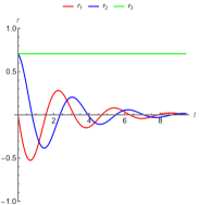
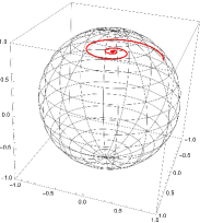
Figure 1: Panel (a): Temporal evolution of the components of the Bloch vector of a two-level system with $H=\omega\sigma_{3}$, according to MID model, with initial condition $\theta=\frac{\pi}{4}$ and $\phi=\frac{\pi}{2}$. Panel (b): the same evolution on the Bloch sphere. The decoherence parameter is set to $\mu=0.1$ and the natural frequency to $\omega=1$.

Overall, we have that for any value of $\mu$, it is possible to select an optimal value of $\omega^{2}t$ so that the signal-to-noise ratio is maximized and maintains the same value. This possibility is a promising outcome, indicating that even very small values of the decoherence parameter may be reliably estimated.

The QFI establishes the upper bound on precision over all possible POVMs. However, it is not guaranteed that the POVM saturating the bound is a practically feasible one. In order to investigate whether it is possible to achieve the maximum precision using a spin measurement, we evaluate the Fisher Information (8) of the generic spin measurement $\left\{\ket{\theta\phi}\bra{\theta\phi},\mathbb{I}-\ket{\theta\phi}\bra{\theta\phi}\right\}$ where $\ket{\theta\phi}=\cos{\frac{\theta}{2}}\ket{0}+e^{i\phi}\sin{\frac{\theta}{2}}\ket{1}$, and $\ket{0}$ and $\ket{1}$ are eigenstates of $\sigma_{3}$. We obtain

$$F=-\frac{1}{S}\left(64t^{2}\omega^{4}\cos^{2}2\omega t\sin^{2}{\theta}\right)$$ (24)

where

$$S= 1-2e^{8t\mu\omega^{2}}(3+\cos{2\theta})+8e^{4t\mu\omega^{2}}\cos^{2}{\theta}\cos 2\omega t$$

$$-2\cos{2\theta}\cos^{2}2\omega t+\cos 4\omega t$$ (25)

By maximizing over $\theta$, we find the optimal spin measurement for $\theta=\frac{\pi}{2}$. We then consider the ratio between the optimal FI and the QFI

$$\frac{F}{Q}=-\frac{2\left(-1+e^{8t\mu\omega^{2}}\right)\cos^{2}2\omega t}{1-2e^{8t\mu\omega^{2}}+\cos 4\omega t}$$ (26)

and observe that it only depends on the two adimensional variables $y=\mu\omega$ and $x=\omega t$. For $x=\pi/2$ the ratio is equal to $1$ for any $y$. The FI is then maximized for $y\simeq 0.127$, which corresponds to the optimal setting to estimate $\mu$. We conclude that, at least in principle, the MID model is amenable to falsification through a spin measurement.

IV.2 Harmonic oscillator

Here we apply the MID model to a free harmonic oscillator, i.e., $H=\omega a^{\dagger}a$, and analyze whether and under which conditions this system is suitable for estimating the value of the dephasing parameter. We start by writing Eq. (1) in the Fock basis

$$\frac{d}{dt}\rho_{nm}=-i\omega(n-m)\rho_{nm}-\mu\omega^{2}(n-m)^{2}\rho_{nm}$$ (27)

which is solved by

$$\rho_{nm}(t)=C_{n}(0)C_{m}^{*}(0)e^{-i\omega(n-m)t-\mu{\omega^{2}(n-m)^{2}t}}$$ (28)

where $C_{n}(0)$ is the amplitude of the initial state along the $m$-th eigenstate of the Hamiltonian and $C_{m}^{*}(0)$ denotes the complex conjugate. In particular, we consider the oscillator initially prepared in a coherent state, i.e.,

$$\ket{\alpha} =e^{-\frac{|\alpha|^{2}}{2}}\sum_{n}\frac{\alpha^{n}\ket{n}}{\sqrt{n!}}$$ (29)

$$C_{nm}(0) =e^{-|\alpha|^{2}}\frac{\alpha^{n}\alpha^{*m}}{\sqrt{n!m!}}\,,$$ (30)

and use Eq. (15) to evaluate the QFI. More specifically, we consider the evolved density matrix, with elements

$$\rho_{mn}=\frac{\alpha^{n}\alpha^{*m}}{\sqrt{n!m!}}e^{-|\alpha|^{2}}e^{-i\omega(n-m)t}e^{-\mu\omega^{2}(n-m)^{2}t}$$ (31)

and diagonalize it by truncating the Hilbert space at dimension $20\times 20$, which ensures normalization in the entire temporal range we have explored. In order to maximize the QFI, we look for its scaling properties. An extensive numerical analysis, corroborated by analytic considerations, reveals that the QFI is a function of two variables only, the coherent amplitude $\alpha$ and the adimensional variable $c=\mu\omega^{2}t$. In Fig. 2 we show the behaviour of the QFI as a function of these two variables. The maximum of the QFI is achieved for $\alpha\simeq 3.16$ and $c\simeq 0.44$, independently of $\mu$, whereas the value of the maximum does depend on $\mu$ and scales as $QFI_{\max}\simeq 0.464/\mu^{2}$. This implies that the quantum signal-to-noise ratio is constant $R(\mu)\simeq 0.464$. This result is relevant since it means that a reasonable estimate of $\mu$ is achievable also when the actual value is very small.

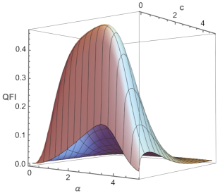
Figure 2: QFI of a harmonic oscillator system, $H=\omega a^{\dagger}a$, evolved according to the MID model. The plot is obtained for $\omega=1$ and $\mu=1$. The QFI depends on the coherence amplitude $\alpha$ and the adimensional variable $c=\mu\omega^{2}t$. The maximum is achieved for $\alpha\simeq 3.16$ and $c\simeq 0.44$, independently of $\mu$, whereas the value of the maximum does depend on $\mu$ and scales as $QFI_{\max}\simeq 0.464/\mu^{2}$.

V Metrology of the GND parameter

Let us now address the non-linear, deterministic, dissipative model suggest by Gisin (GND model) [10] and discuss whether the value of the intrinsic dissipation parameter $\gamma$ may be inferred by monitoring a two-level system or a harmonic oscillator.

V.1 Two-level system

We start from the master equation (3) and write it in the Bloch sphere representation

$$\dot{r_{1}} =-2\omega r_{2}+2\gamma\omega r_{1}r_{3}$$ (32)

$$\dot{r_{2}} =2\omega r_{1}+2\gamma\omega r_{2}r_{3}$$ (33)

$$\dot{r_{3}} =-2\gamma\omega(r_{1}^{2}+r_{2}^{2})\,.$$ (34)

Since in the GND model purity is preserved if we start from a pure state we have $\left|r\right|=1$ at any time. Consequently, the third equation can be rewritten as $\dot{r}_{3}=-2\gamma\omega(1-r_{3}^{2})$, with solution:

$$r_{3}(t)=-1+\frac{2}{D}(1+\cos{\theta})$$ (35)

where $D\equiv 1-e^{4t\gamma\omega}(-1+\cos{\theta})+\cos{\theta}$. Inserting, Eq. (35) in Eq. (34) and assuming a generic initial condition, we arrive at

$$r_{1}(t) =\frac{2}{D}\,e^{2\gamma\omega t}\cos(\phi+2\omega t)\sin{\theta}$$ (36)

$$r_{2}(t) =\frac{2}{D}\,e^{2\gamma\omega t}\sin(\phi+2\omega t)\sin{\theta}$$ (37)

This shows that $r_{1}$ and $r_{2}$ oscillate and vanish exponentially, i.e, coherent decreases with time. Meanwhile, $r_{3}$ approaches -1, i.e., energy is dissipated and the state evolves toward the lowest energy level. Finally, the modulus of the Bloch vector $|\bar{r}|=1$ is constant and remains on the Bloch Sphere surface, i.e. purity is preserved. In Figure (3), we illustrate the evolution of the Bloch vector for $\theta=\frac{\pi}{2}$ and $\phi=0$. The decoherence parameter is set to $\gamma=0.1$, a value significantly larger than the expected one, but chosen to enhance graphic clarity. We have also set $\omega=1$.

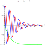
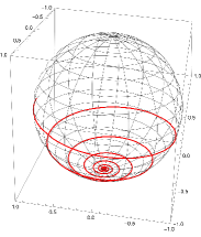
Figure 3: Panel (a): Temporal evolution of the components of the Bloch vector of a two-level system with $H=\omega\sigma_{3}$, according to GND model, with initial condition $\theta=\frac{\pi}{4}$ and $\phi=0$. Panel (b): the same evolution on the Bloch sphere. The decoherence parameter is set to $\gamma=0.1$ and the natural frequency to $\omega=1$.

The density matrix can be written as

$$\rho(t)=\begin{pmatrix}\left[1+e^{4\gamma\omega t}\tan^{2}{\frac{\theta}{2}}\right]^{-1}&D^{-1}\,\sin{\theta}\,e^{-i\phi}\,e^{-2(i-\gamma)\omega t}\\ &\\ D^{-1}\,\sin{\theta}\,e^{i\phi}\,e^{2(i+\gamma)\omega t}&1-\left[1+e^{4\gamma\omega t}\tan^{2}{\frac{\theta}{2}}\right]^{-1}\end{pmatrix}\,,$$ (38)

where we can clearly see the lowest energy level being filled with time. Since the system is pure the QFI may be written as [38]

$$Q(\lambda)=\left|\partial_{\lambda}\bar{r}\right|^{2}\,,$$ (39)

leading to

$$Q(\gamma)=16\omega^{2}t^{2}\,\frac{e^{4\gamma\omega t}\sin^{2}{\theta}}{(1-e^{4t\gamma\omega}(-1+\cos{\theta})+\cos{\theta})^{2}}\,.$$ (40)

The quantum signal-to-noise ratio may be written in terms of the state parameter $\theta$ and of the adimensional variable $x=\gamma\omega t$.

$$R(\gamma,\theta)=16x^{2}\frac{e^{4x}\sin^{2}{\theta}}{(1-e^{4x}(-1+\cos{\theta})+\cos{\theta})^{2}}\,.$$ (41)

The maximum is found for

$$\cos{\theta}=\frac{e^{4\gamma\omega t}-1}{e^{4\gamma\omega t}+1}$$ (42)

and corresponds to the value

$$R(x)=4(\gamma\omega t)^{2}$$ (43)

Since we are working with a monotonically increasing function, it is recommended to select $\gamma\omega t$ as large as experimentally feasible. With this choice, the maximum of $R$ is obtained for vanishing $\theta$. However, we must account for the discontinuity at of the QFI $\theta=0$ where $Q(\gamma)=0$. This discontinuity reflects the physical fact that the eigenstates are stationary under this evolution.

Let us now evaluate the FI of a generic spin measurement. Following the steps already followed in the previous Section we arrive at

$$F=-\frac{4\omega t}{T}\Big{[} \sin 2\theta-\cosh 2\omega t\Big{(}\cosh 2t\gamma\omega\sin 2\theta$$

$$-2\sin\theta\sinh 2t\gamma\omega\Big{)}\Big{]}^{2}$$ (44)

where

$$T= 2\left[\cos 2t\omega-\cosh 2t\gamma\omega\right](3+\cos 2\theta\cosh 2t\gamma\omega$$

$$+ \,4\cos 2t\omega\sin^{2}\theta-8\cos\theta\sinh 2t\gamma\omega\left[\cosh 2t\gamma\omega\right.$$

$$- \left.\cos\theta\sinh 2t\gamma\omega\right]^{2}\,.$$

Upon choosing $\theta$ as in Eq. (42) and $\omega t=k\frac{\pi}{2}$, we have $F=Q$ independently of $\gamma$. However, in order to make $R$ independent of $\gamma$, large values of time $k=\frac{1}{\gamma}$ should be chosen. If this constraint may be fulfilled experimentally, then it would be possible to falsify the GND model through spin measurements.

V.2 Harmonic oscillator

According to Eq. (6), the evolution of a generic state of a harmonic oscillator in the GND model can be written as

$$\ket{\psi_{t}}=\sum_{n}\frac{e^{-(i+\gamma)\omega nt}C_{n}(0)\ket{n}}{\sqrt{\sum_{n}|C_{n}(0)|^{2}e^{-2\gamma\omega nt}}}.$$ (45)

Starting from a coherent state $|\alpha\rangle$, we obtain that the evolved state is still coherent with a decreased amplitude $|\alpha\rangle e^{-\gamma\omega t}$. In addition, since the state is pure, we can calculate the QFI using Eq. (16), arriving at

$$Q(\gamma)=4\omega^{2}t^{2}|\alpha|^{2}e^{-2\gamma\omega t}\,.$$ (46)

The quantum signal-to-noise ratio $R(\gamma)$ is a function of the sole variable $x=\gamma\omega t$ and is maximized for $x=1$. There we have a constant quantum signal-to-ratio $R=4|\alpha|^{2}$, meaning that we may increasing precision by increasing the energy of the probe state.

VI Discussion and conclusions

In Table 1 we summarize the optimal conditions required to maximize the estimability of the intrinsic decoherence parameters of MID and GND models, using a two-level system or a harmonic oscillator.

	MID model	GND model
Two-level	$t\simeq 0.199/(\mu\omega^{2})$ $\theta=\frac{\pi}{2}$ $R\simeq 0.162$	$t\gg 1/\omega$ $\theta=\arccos\left(\frac{e^{4\gamma\omega t}-1}{e^{4\gamma\omega t}+1}\right)$ $R=4(\gamma\omega t)^{2}$
Oscillator	$t\simeq 0.44/(\mu\omega^{2})$ $\alpha\simeq 3.16$ $R\simeq 0.464$	$t=1/(\gamma\omega)$ $\alpha\gg 1$ $R=4|\alpha|^{2}$

Table 1: Summary of the conditions to maximize the estimability of the intrinsic decoherence parameters of MID and GND models

We should notice that for both systems and both models, since the expected values of $\mu$ or $\gamma$ are small, the optimal conditions require a large value of the interaction time, i.e., $t\gg 1/\omega^{2}$ for MID model and $t\gg 1/\omega$ for the GND one. However, one should also take into account the intrinsic decoherence phenomena are expected to occur in a shorter time scale compared to extrinsic ones (see for example [39]) and by performing experiments with an excessively large $t$ we may/should attribute dephasing and dissipation of our system to the interaction with the external environment, rather than to the temporal evolution, making the experiment inconclusive. A possible solution is to employ systems characterized by a large value of $\omega$ and, at least for the GND model, to use a harmonic oscillator prepared in a coherent state with large amplitude.

Another concern may arise about the optimal values of the evolution time, which in principle does depend on the value of the decoherence parameters, which is unknown and is just what we are trying to estimate. We can address this issue by employing an iterative strategy where we initially guess a reasonable value of the parameter, perform measurement in the corresponding optimal conditions and use the estimated value of the parameter to determine renewed and improved conditions. As these conditions should yield a smaller variance, we anticipate obtaining a more accurate value of the parameter for the subsequent step. This iterative process continues, and if we begin with a reasonable value of the decoherence parameter, we should eventually converge to a satisfactory level of precision.

In the cases we examined, the quantum signal-to-noise ratio can remain constant (as in the MID model) or even increase over time or with probe energy (as in the GND model). This is a promising outcome since it suggests that with a sufficiently large number of measurements, it is possible to estimate the IDM parameter with a suitable precision, in turn making the intrinsic decoherence model falsifiable and worth of study to assess their validity.

In conclusion, our primary aim was to assess the testability of two paradigmatic models of intrinsic decoherence. Our results demonstrate that there are optimal conditions under which the MID and GND models can be falsified, i.e., it is possible to conduct experiments to validate or refute those models. Simply put, the IDM may be wrong after all [40].