Experimental single-copy distillation of quantumness from higher-dimensional entanglement

Abstract

Entanglement is at the heart of quantum theory and is responsible for various quantum-enabling technologies. In practice, during its preparation, storage, and distribution to the intended recipients, this valuable quantum resource may suffer from noisy interactions that reduce its usefulness for the desired information-processing tasks. Conventional schemes of entanglement distillation aim to alleviate this problem by performing collective operations on multiple copies of these decohered states and sacrificing some of them to recover Bell pairs. However, for this scheme to work, the states to be distilled should already contain a large enough fraction of maximally entangled states before these collective operations. Not all entangled quantum states meet this premise. Here, by using the paradigmatic family of two-qutrit Werner states as an exemplifying example, we experimentally demonstrate how one may use single-copy local filtering operations to meet this requirement and to recover the quantumness hidden in these higher-dimensional states. Among others, our results provide the first proof-of-principle experimental certification of the Bell-nonlocal properties of these intriguing entangled states, the activation of their usefulness for quantum teleportation, dense coding, and an enhancement of their quantum steerability, and hence usefulness for certain discrimination tasks. Our theoretically established lower bounds on the steering robustness of these states, when they admit a symmetric quasiextension or a bosonic symmetric extension, and when they show hidden dense-codability may also be of independent interest.

Introduction.–Ever since its discovery, quantum entanglement Horodecki et al. (2009) has played a fascinating role in shaping Bell (1964) our understanding of the physical world. In the modern era, entanglement takes the role of a powerful resource, enabling quantum computation Jozsa and Linden (2003); Vidal (2003), quantum-enhanced communications Ekert (1991); Bennett and Wiesner (1992), and quantum metrology Tóth and Apellaniz (2014), etc. To take advantage of these possibilities at a large scale, a quantum internet Wehner et al. (2018) where we can readily perform quantum communications between any two points is clearly desirable. Accordingly, the possibility of distributing entanglement in one way or another (see, e.g., Żukowski et al. (1993); Yin et al. (2017)) will be more than welcome.

Even with ideal preparation, the quality of entanglement can easily degrade over time, either during the storage or distribution stage. Consequently, much effort has been devoted to understanding how one can recover maximally entangled Bell pairs via entanglement distillation or purification protocols Bennett et al. (1996); Deutsch et al. (1996). Indeed, for quantum states violating the reduction criterion Horodecki and Horodecki (1999), iterative single-copy local filtering operations (ScLFs) Gisin (1996) followed by collective local operations Bennett et al. (1996); Horodecki and Horodecki (1999) distill, with a nonzero probability, quantum states having an arbitrarily high Bell-state fidelity.

Nonetheless, some bipartite entangled states, e.g., those having positive-partial-transposition Peres (1996) (PPT), are undistillable Horodecki et al. (1998). There is even evidence DiVincenzo et al. (2000); Dür et al. (2000) suggesting that some non-PPT (NPPT) quantum states, such as the Werner states Werner (1989), are undistillable. Since all two-qubit entangled states are distillable Horodecki et al. (1997), this intriguing phenomenon of bound entanglement Horodecki et al. (1998) only occurs among higher-dimensional (HD) mixed entangled states. In contrast, pure HD entanglement may offer an advantage over its qubit counterparts in entanglement distribution Steinlechner et al. (2017); Ecker et al. (2019); Hu et al. (2020a) and various information-processing tasks (see, e.g., Liu et al. (2002); Liang et al. (2003); Vértesi et al. (2010) for some theoretical proposals).

To date, it remains unknown Horodecki et al. (2022) whether all NPPT entangled states are distillable. Even among those that are distillable, the number of copies required may be arbitrarily large Watrous (2004); Fang and Liu (2020, 2022); Regula (2022). Moreover, to distill via the (generalized) recurrence protocol Bennett et al. (1996); Horodecki and Horodecki (1999), the input state to the protocol must already have a large enough fully-entangled fraction Horodecki et al. (1999) (to the point that it even ensures its usefulness Popescu (1994) for teleportation). To meet this requirement, the initial noisy entangled state may thus have to go through additional ScLFs before being subjected to the collective distillation operations. Even though latter, more technically challenging, operations have been achieved for two copies in various experiments Pan et al. (2001, 2003); Zhao et al. (2003); Yamamoto et al. (2003); Walther et al. (2005); Reichle et al. (2006); Kalb et al. (2017) (see also Hu et al. (2021a); Ecker et al. (2021)), we are still far from recovering a near-to-perfect Bell pair via conventional distillation schemes.

In contrast, for the sake of recovering quantumness or quantum advantage over classical resources in information processing tasks, ScLFs often suffice. For instance, they can help Zhao et al. (2017) distinguish different types of entanglement, recover usefulness for secure communication Singh et al. (2021), unveil hidden Pramanik et al. (2019); Nery et al. (2020); Hao et al. (2024); Zhang et al. (2024) quantum steerability Wiseman et al. (2007); Uola et al. (2020), hidden Li et al. (2021) teleportation power Popescu (1994) (see also Masanes (2006)), as well as the (seemingly) hidden Bell-nonlocality of certain two-qubit states Gisin (1996); Kwiat et al. (2001); Wang et al. (2006, 2020) and HD states Popescu (1995); Kumari (2024) (see also Masanes et al. (2008); Liang et al. (2012)). Here, building on the results from Popescu (1995); Liang et al. (2012); Li et al. (2021), we experimentally demonstrate the activation of various desired properties via the same ScLF for one classic family of HD quantum states—the two-qutrit Werner states. Although tremendous efforts have been devoted to the generation and detection of HD entanglement and their nonlocal properties (see, e.g., Thew et al. (2004); Huber et al. (2010); Schwarz et al. (2016); Martin et al. (2017); Islam et al. (2017); Bavaresco et al. (2018); Zeng et al. (2018); Wang et al. (2018); Hu et al. (2018); Lu et al. (2020); Dada et al. (2011); Hu et al. (2020b, 2021b); Designolle et al. (2021); Qu et al. (2022a, b)), our work gives the first experimental demonstration of the single-copy distillation of quantumness from HD entanglement.

Werner states.–The bipartite $d$-dimensional ($d\geq 2$) Werner state Werner (1989) consists of a convex mixture of the (normalized) projectors $\Pi_{\pm}\equiv\frac{1}{2}\left(\mathbb{I}_{d^{2}}\pm V\right)$ onto the symmetric ($+$) and anti-symmetric ($-$) subspace:

$$W^{(d)}(v):=\frac{v}{n_{+}^{d}}\Pi_{+}^{d}+\frac{1-v}{n_{-}^{d}}\Pi_{-}^{d},\quad v\in\left[0,1\right],$$ (1)

where $\mathbb{I}_{d^{2}}$ is the identity operator acting on $\mathbb{C}^{d}\otimes\mathbb{C}^{d}$, $n_{\pm}^{d}:={\rm tr}\Pi_{\pm}^{d}=\frac{d(d\pm 1)}{2}$ and $V$ is the swap operator, i.e., $V|\psi\rangle_{A}|\phi\rangle_{B}=|\phi\rangle_{A}|\psi\rangle_{B}$ for all $|\psi\rangle,|\phi\rangle\in\mathbb{C}^{d}$. $W^{(d)}(v)$ are PPT Dür et al. (2000) and separable Werner (1989) if and only if (iff ) $v\geq\frac{1}{2}$. However, entangled Werner states are only known to be distillable when Dür et al. (2000); DiVincenzo et al. (2000) $v<v_{\text{distill}}\equiv\frac{d+1}{4d-2}$. In this regard, a state $\rho$ is said to be distillable Horodecki and Horodecki (2001) if it is $k$-distillable for some natural number $k$, i.e., if there exists qubit projectors $\Pi_{A},\Pi_{B}$ such that $\frac{\Pi_{A}\otimes\Pi_{B}\rho^{\otimes k}\Pi_{A}\otimes\Pi_{B}}{{\rm tr}(\Pi_{A}\otimes\Pi_{B}\rho^{\otimes k}\Pi_{A}\otimes\Pi_{B})}$ is entangled. To determine the existence of NPPT bound entangled states Horodecki et al. (2022), it suffices Dür et al. (2000) to consider $W^{(d)}(v)$ for $d>2$.

HD Werner states are peculiar, however, not only because of their distillability properties but also because they are useless in various tasks. Indeed, all HD $W^{(d)}(v)$’s satisfy the reduction criterion (RC) of separability Horodecki and Horodecki (1999). Consequently, even those that are distillable cannot be fed directly to the generalized recurrence protocol Horodecki and Horodecki (1999) for entanglement distillation. Their compliance with RC also renders them useless for quantum teleportation Horodecki and Horodecki (1999) and superdense coding Bruß et al. (2004). However, as shown in Li et al. (2021), an appropriate ScLF (in the form of qubit projection) can activate their usefulness for teleportation whenever $v<v_{\text{distill}}$.

Furthermore, Werner states with $v\geq v_{\text{steer}}\equiv\frac{d+1}{2d^{2}}$ are the first known examples of entangled quantum states not violating any Bell Werner (1989) or steering Wiseman et al. (2007) inequality with projective measurements (see Fig. 1). However, Popescu Popescu (1995) showed that after a successful qubit ScLF, it is possible for $W^{(d\geq 5)}(v_{\text{steer}})$ to violate the Clauser-Horne-Shimony-Holt (CHSH) Bell inequality Clauser et al. (1969). More generally, $W^{(d)}(v)$’s are known (Johnson and Viola, 2013, Theorem 6) to admit a symmetric $(1,k)$ or $(k,1)$-extension Terhal et al. (2003); Doherty et al. (2002) iff $v\geq v_{\text{Sym}}\equiv\frac{1}{2}\left(1-\frac{d-1}{k}\right)$. In other words, for these states, there exists a $(1+k)$-partite qudit state $\rho$ that recovers $W^{(d)}(v)$ after tracing out any $(k-1)$ copies of Alice’s (Bob’s) subsystems. It then follows Terhal et al. (2003) that $W^{(d)}(v)$ for $v\geq v_{\text{Sym}}$ cannot violate any Bell inequality with $\min\{s_{a},s_{b}\}\leq k$ where $s_{a}$ ($s_{b}$) is the number of measurement settings for Alice (Bob). In particular, since $v_{\text{Sym}}$ vanishes when $k=d-1$, $W^{(d)}(v)$ satisfy Terhal et al. (2003) all Bell inequalities with $d-1$ or fewer measurement bases at one side. For example, all two-qutrit Werner states cannot violate any two-or-fewer-setting Bell inequality on one side. Again, a qubit ScLF reveals Liang et al. (2012) the Bell-nonlocality (possibly) hidden in some of these states, which we demonstrate experimentally in this work.

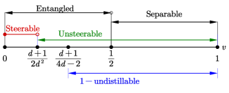
Figure 1: Werner states $W^{(d)}(v)$, $v\in[0,1]$ is entangled iff $v<\frac{1}{2}$, 1-distillable (steerable with projective measurements) when $0\leq v<v_{\text{distill}}$ ($0\leq v<v_{\text{steer}}$), where $v_{\text{steer}}=\frac{d+1}{2d^{2}}<v_{\text{distill}}=\frac{d+1}{4d-2}$. For $d>2$, all $W^{(d)}(v)$ are useless for teleportation, dense-coding, and not known to violate Bell inequality.

How does a qubit ScLF enable the distillation of many of these useful properties? We can gain some intuition into this by first noting that $\Pi_{+}^{d}+\Pi_{-}^{d}=\mathbb{I}_{d^{2}}$ and Popescu (1995) $\Pi_{-}^{d}=\sum_{i<j}\varrho_{0}^{i,j}$ where $\varrho_{0}^{i,j}=|\Psi^{-}_{i,j}\rangle\!\langle\Psi^{-}_{i,j}|$ is a singlet projector defined on the two-qubit subspace $\mathcal{H}_{i,j}:=\text{span}\{|k\ell\rangle:=|k\rangle|\ell\rangle\}_{k,\ell=i,j}$. Then, by defining $p:=\frac{1}{d}$, $q:=1-\frac{2d}{d+1}v$, and noting that $n_{-}^{d}$ is also the binomial coefficient of $d$ chooses 2, we can rewrite $W^{(d)}(v)$ as a uniform mixture of two-qubit states $\varrho^{i,j}$:

$$W^{(d)}(q)=\frac{q}{n_{-}^{d}}\sum_{i<j}\varrho_{0}^{i,j}+\frac{1-q}{d^{2}}\mathbb{I}_{d^{2}}=\frac{1}{n_{-}^{d}}\sum_{i<j}\varrho^{i,j},$$ (2a)

$$\varrho^{i,j}(q):=q\varrho_{0}^{i,j}+\left(1-q\right)\left[p\varrho_{1}^{i,j}+\left(1-p\right)\varrho_{2}^{i,j}\right],$$ (2b)

where $\varrho_{1}^{i,j}=\frac{|ii\rangle\!\langle ii|+|jj\rangle\!\langle jj|}{2}$, $\varrho_{2}^{i,j}=\frac{|ij\rangle\!\langle ij|+|ji\rangle\!\langle ji|}{2}$. In this decomposition, only the two-qubit singlet projectors $\{\varrho_{0}^{i,j}\}_{i,j}$ contribute to the entanglement of $W^{(d)}(v)$. The act of a qubit projection, say, $\Pi_{2}:=|0\rangle\!\langle 0|+|1\rangle\!\langle 1|$, on both sides then keeps the maximally entangled $\varrho_{0}^{0,1}$ and the separable $\frac{\mathbb{I}_{4}}{4}$ with some probability while getting rid of the remaining components in all other two-qubit subspaces, thereby effectively “purifying” the entanglement contained in $W^{(d)}(v)$. From Eq. 2a, we see that upon a successful qubit projection, since $\Pi_{2}\otimes\Pi_{2}W^{(d)}(v)\Pi_{2}\otimes\Pi_{2}\propto W^{(d=2)}(v^{\prime})$, we obtain a two-qubit Werner state with a symmetric weight $v^{\prime}=\frac{3(d-1)v}{(d+1)(1-v)+3(d-1)v}$. Note that $v^{\prime}\geq v$ for all $d>2$.

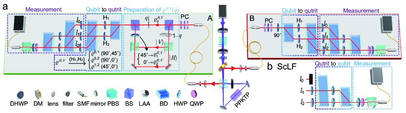
Figure 2: a. Experimental setup to generate $W^{(d=3)}(v)$. We first generate polarization-entangled photons, each coupled into a single-mode fiber (SMF) and sent to Alice and Bob. The fiber-induced polarization drift is corrected by a polarization controller (PC), which is a half-wave plate (HWP) sandwiched by two quarter-wave plates (QWPs). Then, we partially decohere $\varrho^{H,V}_{0}$ to prepare the state $\varrho^{H,V}(q)$. Finally, $\varrho^{H,V}(q)$ is mapped to $W^{(d=3)}(v)$ encoded in the path DOF with two optical networks, each consisting of two BDs and two HWPs, where the parameter $v$ is adjustable via $q$ by rotating two Linear-Adjustable Attenuators (LAAs). b. Realization of the ScLF. Optical elements list. DHWP: dual-wavelength HWP@ 405 & 810 nm. DM: dichroic mirror. NBF: narrow-band filter. PBS: polarizing beam splitter. BS: beam splitter. BD: beam displacer. More details are provided in Appendix A.

Experimental Werner states and filtering operation.–The decomposition of Eq. 2 not only sheds light on the relevance of a qubit ScLF but also provides a systematic way for preparing an entangled $W^{(d)}(v)$ for an arbitrary $d$ via generating and mixing the various two-qubit states $\varrho^{i,j}(q)$ residing in $\mathcal{H}_{i,j}$. To this end, we start by preparing a pair of maximally entangled photons in the polarization degree of freedom (DOF) $|\Psi^{+}\rangle_{\text{AB}}=\frac{1}{\sqrt{2}}(|H\rangle|V\rangle+|V\rangle|H\rangle)_{\text{AB}}$, where $H$ and $V$ denote, respectively, horizontal and vertical polarization. As shown in Fig. 2a, the entangled photons are generated via the spontaneous parameter down conversion process (SPDC) from a periodically-poled potassium titanyl phosphate (PPKTP) crystal in a Sagnac interferometer, which is bidirectionally pumped by a laser with central wavelength at 405 nm. By setting a HWP at 0^∘ on photon B, $|\Psi^{+}\rangle_{\text{AB}}$ is transformed into $\varrho_{0}^{H,V}=|\Psi^{-}\rangle_{\text{AB}}\langle\Psi^{-}|$. Then, we use two BSs, two PBSs and two tunable LAAs (with transmittance of $q$ and $1-q$, respectively) to partially decohere $\varrho_{0}^{H,V}$ and prepare the mixed state $\varrho^{H,V}(q)$ in Eq. 2 by randomly rotating a HWP between $45^{\circ}$ and $0^{\circ}$. Finally, we obtain the $d$-dimensional Werner states $W^{(d)}(v)$ from $\varrho^{H,V}(q)$ with a qubit-to-qudit mapping, where the qudit is encoded in the path DOF $\{|l_{k}\rangle\}$ and the mapping is achieved with two optical networks each consisting of $d-1$ beam displacers (BDs) and a series of HWPs on photon A and B. For $d=3$ in this work, we use two BDs and two HWPs at each side (as shown in Fig. 2a) to prepare eleven $W^{(d=3)}(v)$ with $v\in[0,0.5]$ in steps of 0.05. See Appendix A.2 for further details.

We reconstruct the prepared $\rho_{\text{expt}}(v)$ using quantum state tomography (QST), in which an iterative maximum-likelihood algorithm Altepeter et al. (2005) is performed on the twofold coincidence collected in $9\times 9$ measurement basis vectors (see Section A.3). We then calculate the reconstructed $\rho_{\text{expt}}(v)$’s fidelity with respect to $W^{(d=3)}(v)$, and find that they range approximately from $0.958$ to $0.995$ (see Table 4). Also, we confirm the entanglement of $\rho_{\text{expt}}(v)$ for $v\leq 0.45$ from their NPPT property (Fig. 3, $\vartriangleright$) and the 1-distillability Dür et al. (2000) of $\rho_{\text{expt}}(v)$ for $v\leq 0.4$ by showing that, upon optimizing over Schmidt-rank-2 pure state $|\psi\rangle$, $\text{min}_{|\psi\rangle}\left[\langle\psi|\rho_{\text{expt}}^{\text{T}_{A}}(v)|\psi\rangle\right]<0$ (see Fig. 3, $\vartriangleleft$); here, $(.)^{\text{T}_{A}}$ is the partial transposition with respect to $A$. Furthermore, we verify the separability of $\rho_{\text{expt}}(v=0.5)$ by recalling from (Gurvits and Barnum, 2002, Corollary 3) that if $\rho$ acting on $\mathbb{C}^{d}\otimes\mathbb{C}^{d}$ satisfies $\|\rho-\frac{\mathbb{I}_{d^{2}}}{d^{2}}\|_{2}^{2}\leqslant\frac{1}{d^{2}(d^{2}-1)}$, then it is separable. These results are in good agreement with the theoretical predictions except that $\rho_{\text{expt}}(v=0.4)$ appears to be 1-distillable while $W^{(d=3)}(v=0.4)$ is not.

ScLF and distillation of quantumness.–With our encoding of the quantum information, a qubit filtering—relevant for distilling the various quantum features alluded to above—is straightforward. As shown in Fig. 2b, to keep only contributions to the two lower optical paths $\{|l_{1}\rangle,|l_{2}\rangle\}$, we block the light propagating through the upper optical path $|l_{0}\rangle$. After ScLF, the two-qubit state $\rho_{\text{expt},f}(v)$ encoded in $\{|l_{1}\rangle,|l_{2}\rangle\}$ is mapped back to the polarization DOF and then reconstructed using a HWP, a QWP and a PBS, and their fidelity ranges roughly from 0.934 to 0.995, cf. Table 4. In the following, we compare the properties of $\rho_{\text{expt}}(v)$ and $\rho_{\text{expt},f}(v)$ to illustrate how ScLF has enabled the recovery of quantum features missing in $\rho_{\text{expt}}(v)$.

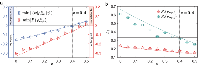
Figure 3: a. Experimental results confirming the entanglement and 1-distillability of the experimentally prepared Werner states $\rho_{\text{expt}}(v)$. The red right triangle $\vartriangleright$ gives the minimum eigenvalue of $\rho_{\text{expt}}^{\text{T}_{A}}$, where a negative (non-negative) value confirms entanglement (undistillability). Similarly, a negative (non-negative) value for the blue triangle $\vartriangleright$ confirms distillability (1-undistillability). See text for details. The vertical dashed line marks the 1-distillability boundary. b.  Theoretical (dashed lines) and experimental (dots) results illustrating the teleportation power before and after applying the qubit ScLF on $\rho_{\text{expt}}(v)$. The bottom (red) results correspond to the unfiltered states $W^{(d=3)}(v)$ and $\rho_{\text{expt}}(v)$ (experiment), while the top (green square) results are for the filtered state $W^{(d=3)}_{f}(v)$ and $\rho_{\text{expt},f}(v)$ (experiment). The solid black line is the classical threshold $F^{c}_{d=3}=\frac{1}{3}$ and the vertical dashed line marks the boundary of usefulness for teleportation.

We begin with the Bell-nonlocality property of these states. Except for $\rho_{\text{expt}}(v=0)$, which is not even 2-quasiextendible, all other $\rho_{\text{expt}}(v)$ are found to be symmetric $(1,k)$ or $(k,1)$ quasi-extendible iff the corresponding $W^{(d)}(v)$ are. Hence, $\rho_{\text{expt}}(v)$ with $v\geq\frac{1}{2}(1-\frac{2}{k})\neq 0$ cannot violate any Bell inequalities with only $k$ or fewer measurement bases. In fact, despite extensive numerical optimizations, we do not find a Bell-inequality violation by any of the entangled $\rho_{\text{expt}}(v)$; see Section B.1.2. In contrast, using the Horodecki criterion Horodecki et al. (1995), the filtered states $\rho_{\text{expt},f}(v)$ are easily verified to give a maximal CHSH-Bell violation Clauser et al. (1969) of $\mathcal{S}_{\text{\tiny CHSH}}=2.65\pm 0.02,2.46\pm 0.01,2.02\pm 0.02$, and $2.01\pm 0.01$ for $v=0,0.05,0.10$, and $0.15$, respectively, in agreement with the results derived for $W^{(d)}(v)$ Liang et al. (2012). Note, however, that $\rho_{\text{expt},f}(v=0.1)$ and $\rho_{\text{expt},f}(v=0.15)$ violates the CHSH-Bell inequality (with a Bell-local bound of $\mathcal{S}_{\text{\tiny CHSH}}=2$) by less than one standard deviation.

Next, recall from Horodecki et al. (1999) that the usefulness of a quantum state $\rho$ for teleporting an unknown two-qudit state can be confirmed by verifying that its fully entangled fraction:

$$F_{d}(\rho)=\max_{|\Psi_{d}\rangle}\langle\Psi_{d}|\rho|\Psi_{d}\rangle,$$ (3)

is larger than $F^{c}_{d}=\frac{1}{d}$, where $|\Psi_{d}\rangle=(\mathbb{I}_{d}\otimes U_{d})|\Phi^{+}_{d}\rangle$ is an arbitrary maximally entangled two-qudit state, $|\Phi^{+}_{d}\rangle=\frac{1}{\sqrt{d}}\sum_{i=0}^{d-1}|i\rangle|i\rangle$, while $\mathbb{I}_{d}$ and $U_{d}$ are the identity and an arbitrary unitary matrix acting on $\mathbb{C}^{d}$, respectively. From Eq. 3, one can easily verify that if a two-qubit state $\rho$ satisfies $F_{2}>\frac{1}{2}$, it must also satisfy $F_{d}>\frac{1}{d}$ for all integer $d>2$. Since all two-qubit states violating the CHSH-Bell inequality satisfy Horodecki et al. (1996) $F_{2}>\frac{1}{2}$, the CHSH-Bell violation of $\rho_{\text{expt},f}(v)$ for $v\leq 0.15$ already confirm their usefulness for teleporting a qubit state, and hence an arbitrary qudit state. In fact, by using Eq. 3 and the explicit form of $\rho_{\text{expt},f}(v)$, we see from Fig. 3b that the teleportation power of all $\rho_{\text{expt}}(v)$ with $v<v_{\text{distill}}$ is successfully recovered via our qubit ScLF, in agreement with the results of Li et al. (2021). In Section B.3, we show that the same ScLF also activates the dense-codability Bruß et al. (2004) of some $W^{(d)}(v)$ and provide experimental evidence in Section C.3 confirming these findings.

Finally, let us compare the steering robustness Uola et al. (2020) SR—a quantifier of steerability monotonously related Piani and Watrous (2015) to the usefulness of a state for some specific subchannel discrimination task—between $\rho_{\text{expt}}(v)$ and $\rho_{\text{expt},f}(v)$. To our knowledge, the exact value of $\text{SR}[W^{(d)}(v)]$ is unknown. In Appendix B.2, we provide the best lower bound on $\text{SR}[W^{(d)}(v)]$ that we have found using the technique of Cavalcanti and Skrzypczyk (2017) by considering up to $n_{s}=7$ measurement bases. Accordingly, we see in Fig. 4 an improvement from these lower bounds on $\text{SR}[\rho_{\text{expt}}(v)]$ to $\text{SR}[\rho_{\text{expt},f}(v)]$ for all $v<0.25$. In particular, the steerability of $\rho_{\text{expt},f}(v)$ for $v=0.2$ is clearly witnessed while that of $\rho_{\text{expt}}(v)$ is unknown. Note further from Fig. 4 that, in principle, steerability may also be activated beyond $v>v_{\text{steer}}=\frac{2}{9}$ for $d=3$. However, due to experimental imperfections, we do not observe the activation for $v=0.25$.

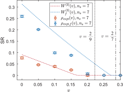
Figure 4: Best lower bound on the steering robustness SR found for $W^{(3)}(v)$, $W^{(3)}_{f}(v)$ [the state obtained from $W^{(3)}(v)$ via qubit ScLF], and their experimental counterparts $\rho_{\text{expt}}(v)$ and $\rho_{\text{expt},f}(v)$. The vertical dashed (dashed-dotted) line at $v=\frac{2}{9}$ ($v=\frac{2}{7}$) marks the boundary of unsteerability with projective measurements before (after) filtering. See Sections B.2 and C.2 for details.

Conclusion.–Using qubit local filtering operations, we experimentally demonstrate the single-copy distillation of several genuine quantum features from the paradigmatic family of higher-dimensional (specifically two-qutrit) Werner states. Notice that via the coordinated local operations of $U\otimes U$-twirling, we can always transform any bipartite quantum state to a Werner state. Thus, in principle, our experimental demonstration of single-copy distillation also applies to all quantum states that transform to a 1-distillable two-qutrit Werner state by these local operations. In turn, our work also demonstrates the single-copy operation involved in the entanglement distillation of higher-dimensional quantum states via Werner states.

To facilitate the experimental preparation of Werner states, we provide an intuitive decomposition of any finite-dimensional Werner states as a mixture of two-qubit states (see also Section A.5). The decomposition, in turn, sheds light on the relevance of qubit filtering operations for these states, partially addressing one of the open problems from Li et al. (2021). Conceivably, our scheme for converting qubit states to higher-dimensional states may also find applications in the experimental preparation of other higher-dimensional states admitting a similar two-qubit decomposition.

Among the various quantum features distilled from the experimentally prepared two-qutrit Werner states, their Bell nonlocality is especially noteworthy. Indeed, our work provides the first proof-of-principle certification of the Bell nonlocality of these important higher-dimensional entangled states, hidden or otherwise. Despite experimental imperfections, we have also recovered the teleportation power for the experimentally prepared 1-distillable two-qutrit Werner states. Using the lower bound on steering robustness we have established theoretically (see Section B.2), our experimental results also provide strong evidence for enhancing steering robustness (and hence usefulness for certain discrimination tasks Piani and Watrous (2015)) via single-copy distillation. Note that the former theoretical results may also be of independent interest, e.g., in the studies of measurement incompatibility Chen et al. (2016).

For future work, within the realm of single-copy local filtering operations, it is clearly of interest to experimentally demonstrate the hidden nonlocality of the five-dimensional Werner states, first discussed in Popescu (1995), and the hidden steerability of the three-dimensional Werner states we barely miss in the current experiment. Since the filtered two-qubit state only exhibits a tiny amount of Bell-nonlocality (steerability), the challenges here are to produce very high-quality, high-dimensional Werner states and follow up with extremely well-controlled qubit projections (and measurements). Another closely related problem worth exploring is the power of local filtering operations beyond a qubit projection.

For example, could a higher-dimensional local filtering operation be more effective, e.g., in demonstrating the hidden nonlocality of $W^{(d)}(v)$ for a broader range of the parameter $v$? A systematic investigation of the problem is surely welcome. Similarly, suppose a more efficient high-dimensional local filtering operation exists to activate dense codability. In that case, the advantage gained in these operations might outweigh the need for classical communication in implementing such operations, thereby overcoming the objection raised in Bruß et al. (2004) for allowing such operations in the characterization of dense-codability. An analytic proof confirming our numerical observation of when a Werner state admits a quasi-symmetric extension or a bosonic symmetric extension is desirable, too.

Appendix A Experimental details

Here, we provide further descriptions of our experimental setup. In our experiment, the Jones matrix $U_{\text{\tiny HWP}}$ $(U_{\text{\tiny QWP}})$ of the half (quarter)-wave plate is a unitary:

$$U_{\text{\tiny HWP}}(\theta) =-\left(\begin{array}[]{cc}\cos 2\theta&\sin 2\theta\\ \sin 2\theta&-\cos 2\theta\end{array}\right),$$ (4)

$$U_{\text{\tiny QWP}}(\theta) =\frac{1}{\sqrt{2}}\left(\begin{array}[]{cc}1+i\cos 2\theta&i\sin 2\theta\\ i\sin 2\theta&1-i\cos 2\theta\end{array}\right).$$

where $\theta$ is the angle between the fast axis and the vertical direction. The global phase in front of $U_{\text{\tiny HWP}}$ can be ignored because a HWP is present in each path of the experimental setups. To follow the subsequent discussions, we remind the readers that a PBS (BD) transmits a photon with horizontal (vertical) polarization but reflects (deviates) one with vertical (horizontal) polarization.

A.1 Entanglement source

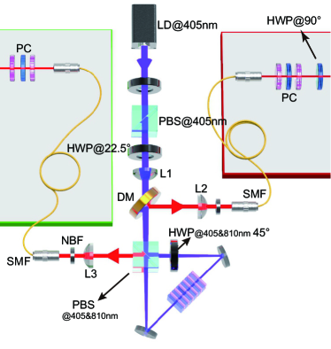
Figure 5: Zoom-in view of the “Entanglement source” part of the experimental setup shown in Fig. 2a for generating maximally entangled photon pairs.

This part, as shown in Fig. 5, aims to generate a maximally entangled state in the form of $|\Psi^{+}\rangle_{\text{AB}}=\frac{1}{\sqrt{2}}(|H\rangle|V\rangle+|V\rangle|H\rangle)_{\text{AB}}$. The polarization of $405$ nm pump light from a laser diode (LD) is set at $|H_{p}\rangle$ with a HWP and a PBS, where the HWP is used to adjust the power intensity of pump light. Then, we use the second HWP set at 22.5^∘, $|H_{p}\rangle$ to rotate polarization, i.e., $|+_{p}\rangle=\frac{1}{\sqrt{2}}(|H_{p}\rangle+|V_{p}\rangle)$. Subsequently, the pump beam is focused into a PPKTP crystal with a beam waist of 74 $\mu$m by two lenses L₁ with focal lengths of $75$ mm and $125$ mm, respectively. The PPKTP crystal with a poling period of $\Lambda=10.025~{}\mu$m is held in a copper oven with its temperature controlled by a temperature controller set at $29^{\circ}$C to realize the optimum type-II quasi-phase matching at $810$ nm.

After passing through a dichroic mirror, the pump beam arrives at a dual-wavelength PBS, where it is converged by lenses and split by the PBS to pump the PPKTP crystal coherently in both the clockwise and counterclockwise directions. The clockwise- and counterclockwise-propagating photons are then recombined by the dual-wavelength PBS to generate polarization-entangled photon pairs with the ideal form of $|\Psi^{+}\rangle_{\text{AB}}=\frac{1}{\sqrt{2}}(|H\rangle|V\rangle+|V\rangle|H\rangle)_{\text{AB}}$. These photons are then filtered by a narrow band filter (NBF) with a full width at half maximum (FWHM) of $3$ nm and each coupled into a single-mode fiber (SMF) by lenses with focal length of $200$ mm (L₂ and L₃) and objective lenses.

For our experiment, the power intensity of pump light is set at $5$ mW, and we observe a twofold coincidence count rate of 73 kHz. The two photons are coupled out by two collimators, and the polarization of each photon is corrected by polarization controller (PC) consisting two QWPs and a HWP. Finally, we let photon B go through an additional HWP at 90^∘ to produce the singlet state $\varrho_{0}^{H,V}=(|\Psi^{-}\rangle\!\langle\Psi^{-}|)_{\text{AB}}$, where $|\Psi^{-}\rangle_{\text{AB}}=\frac{1}{\sqrt{2}}|H\rangle|V\rangle-|V\rangle|H\rangle)_{\text{AB}}$.

A.2 Two-qutrit Werner state preparation

Using the singlet state $\varrho_{0}^{H,V}$, we can further prepare the state $\varrho_{2}^{H,V}=\frac{|HV\rangle\!\langle HV|+|VH\rangle\!\langle VH|}{2}$ by decohering $\varrho_{0}^{H,V}$ in the $\{|H\rangle,|V\rangle\}$ basis, and obtaining therefrom the state $\varrho_{1}^{H,V}=\frac{|HH\rangle\!\langle HH|+|VV\rangle\!\langle VV|}{2}$ via the bit-flip operation $|H\rangle\leftrightarrow|V\rangle$ on one side. Indeed, photons traveling through different paths $R_{1}$, $R_{2}$, and $T$ (see Fig. 6) form an incoherent mixture because the time difference between them exceeds their coherence length. Specifically, the two mixed states $\varrho_{1}^{H,V}$ and $\varrho_{2}^{H,V}$ can be generated when the HWP after PBS₂ is set at $\theta_{1}=45^{\circ}$ and $\theta_{2}=0^{\circ}$, respectively. The step-by-step calculation leading from $\varrho_{0}^{H,V}$ to the two $\varrho_{k}^{H,V}$’s is as follows:

$$\begin{split}|\Psi^{-}\rangle_{\text{AB}}&=\frac{1}{\sqrt{2}}(|HV\rangle-|VH\rangle)_{\text{AB}}\\ &\xrightarrow[\text{photon A}]{\text{PBS}_{1}}\frac{1}{\sqrt{2}}(|HV\rangle|R_{1}\rangle-|VH\rangle|R_{2}\rangle)_{\text{AB}}\\ &\xrightarrow[\text{photon A}]{\text{PBS}_{2}}\frac{1}{2}(|HV\rangle\!\langle HV|+|VH\rangle\!\langle VH|)_{\text{AB}}\\ &\xrightarrow[\text{photon A}]{\text{HWP}~{}@~{}\theta_{k}(t_{k})}\varrho_{k}^{H,V}.\end{split}$$ (5)

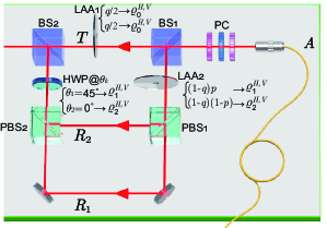
Figure 6: Experimental setup that generates the mixed state of Eq. 6, where the different components are distinguishable by their temporal DOF. To generate $p\varrho_{1}^{H,V}+(1-p)\varrho_{2}^{H,V}$, we randomly set a HWP at 45^∘ or 0^∘ and attenuate the beam accordingly by changing the LAA₂ setting.

After mixing the states prepared through different path lengths and at different times, we obtain the desired polarization-encoded two-qubit mixed states

$$\varrho^{H,V}(q)=q\varrho_{0}^{H,V}+(1-q)\left[p\varrho_{1}^{H,V}+(1-p)\varrho_{2}^{H,V}\right],$$ (6)

where the mixing parameters $q=1-\frac{2d}{d+1}v$ and $p=\frac{1}{d}$ are achieved by adjusting the LAA₁ and LAA₂ according to the transmittance of the tested light through the different paths.

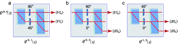
Figure 7: Experimental setups to introduce the path DOF and produce $\rho_{\text{expt}}$, which is a uniform mixture of $\varrho^{0,1}$, $\varrho^{0,2}$, and $\varrho^{1,2}$. The different configurations of HWP in a, b, and c result in photons exiting from the BD via different paths. We encode the current paths with the corresponding polarization $|Vl_{0}\rangle$, $|Hl_{1}\rangle$ or $|Vl_{1}\rangle$ and $|Hl_{2}\rangle$, respectively, as $|0\rangle$, $|1\rangle$ and $|2\rangle$.

Via an appropriate combination of BDs and HWPs, we can convert the polarization-encoded $\varrho^{H,V}(q)$ to a two-qubit state $\varrho^{i,j}(q)$ encoded in the $i$-th and $j$-th path DOF. Mixing them uniformly then gives the desired $d$-dimensional Werner state:

$$W^{(d)}(q)=\frac{2}{d(d-1)}\sum_{i<j}\varrho^{i,j}(q).$$ (7)

Consider, e.g., the preparation of the two-qutrit Werner states shown in Fig. 7. We adjust the HWPs at both A and B to inject $\varrho^{H,V}$ into $\binom{3}{2}$ different paths at each time. Then, mixing uniformly the states $\varrho^{0,1}$, $\varrho^{0,2}$, and $\varrho^{1,2}$ prepared at different times give an ensemble corresponding to Eq. 7 for $d=3$. The detailed preparation process is shown in Fig. 7. Specifically, using the HWP settings of Fig. 7a, Fig. 7b, and Fig. 7c, respectively, the horizontally (vertically) polarized photons will exit from the last BD via path $l_{1}(l_{0})$, $l_{2}(l_{0})$, and $l_{2}(l_{1})$. Together, their average gives the desired $\rho_{\text{expt}}$ encoded in the spatial modes $\{|l_{k}\rangle\}_{k=0,1,2}$.

A.3 Measurement of the two-qutrit Werner states

Note that by construction and the nature of BD, in every single run, the local photonic quantum states that appear in each path $l_{k}$ always come with a definite polarization:

$$l_{0}\leftrightarrow|V\rangle,\quad l_{1}\leftrightarrow|V\rangle\text{ or }|H\rangle,\quad l_{2}\leftrightarrow|H\rangle.$$ (8)

Even when the photon exits via $l_{1}$, we know by construction whether the corresponding photonic polarization state is $|V\rangle$ or $|H\rangle$. Since the polarization DOF is decoupled from the spatial DOF and each term in the sum in Eq. 7 involves only two of the spatial modes (see Fig. 7), we can rely on polarization measurements to realize any qutrit measurement relevant to our experiment.

To this end, the path-encoded qutrit state is analyzed through a measurement device consisting of six HWPs, two BDs, one QWP, and one PBS (see Fig. 8). For QST, we perform an overcomplete set of path measurements with nine basis vectors via the correspondence of Eq. 8:

$$\begin{gathered}\text{M1}:~{}|0\rangle,\quad\text{M2}:~{}|1\rangle,\quad\text{M3}:~{}|2\rangle,\\ \text{M4}:~{}1/\sqrt{2}(|0\rangle+|1\rangle),\quad\text{M5}:~{}1/\sqrt{2}(|0\rangle+i|1\rangle),\\ \text{M6}:~{}1/\sqrt{2}(|0\rangle+|2\rangle),\quad\text{M7}:~{}1/\sqrt{2}(|0\rangle+i|2\rangle),\\ \text{M8}:~{}1/\sqrt{2}(|1\rangle+|2\rangle),\quad\text{M9}:~{}1/\sqrt{2}(|1\rangle+i|2\rangle).\end{gathered}$$ (9)

In particular, the wave plate settings needed to perform a projection onto the individual states of Eq. 9 are shown in Table 1. Note that the HWPs H3, H4, and H5 remove the original polarization information and measure the path information at the same time. Therefore, the HWP H4 should be set according to the polarization of the photon traveling through path $l_{1}$ while the HWP H3 and H5 may be set, without loss of generality, at $45^{\circ}$. For example, if we want to measure M2, H4 should be set to $0^{\circ}$ for $|Hl_{1}\rangle$ and $45^{\circ}$ for $|Vl_{1}\rangle$. Then, the light will pass through the HWP H7 in both cases. From the collection of $9\times 9$ twofold coincidence counts, we reconstruct our density matrix using an iterative maximum-likelihood algorithm Altepeter et al. (2005).

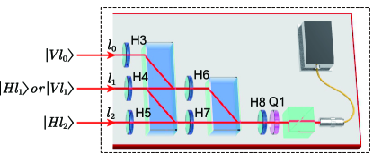
Figure 8: Experimental setups that measure the path information encoded in our qutrit photon contain six HWPs, two BDs, one QWP, a PBS, and a detector. Corresponding to the preparation of the state, we mark the optical paths during the measurement as $l_{0}$, $l_{1}$, and $l_{2}$.

Table 1: Waveplates settings in Fig. 8 to achieve a single qutrit measurement. $\theta$ means that the plate can be set at any angle, but for simplicity, we can always set HWP at $45^{\circ}$. The first (second) entry in the third column is the setting

for a $|H\rangle$ ($|V\rangle$) photon traveling through $l_{1}$. Basis vector H3 H4 ($H$; $V$) H5 H6 H7 H8 Q1 M1 $45^{\circ}$ $\theta$ $\theta$ $0^{\circ}$ $\theta$ $0^{\circ}$ $0^{\circ}$ M2 $\theta$ $0^{\circ}\text{; }45^{\circ}$ $\theta$ $\theta$ $45^{\circ}$ $45^{\circ}$ $0^{\circ}$ M3 $\theta$ $\theta$ $45^{\circ}$ $\theta$ $90^{\circ}$ $45^{\circ}$ $0^{\circ}$ M4 $45^{\circ}$ $0^{\circ}\text{; }45^{\circ}$ $\theta$ $0^{\circ}$ $45^{\circ}$ $22.5^{\circ}$ $0^{\circ}$ M5 $45^{\circ}$ $0^{\circ}\text{; }45^{\circ}$ $\theta$ $0^{\circ}$ $45^{\circ}$ $0^{\circ}$ $45^{\circ}$ M6 $45^{\circ}$ $\theta$ $45^{\circ}$ $0^{\circ}$ $90^{\circ}$ $22.5^{\circ}$ $0^{\circ}$ M7 $45^{\circ}$ $\theta$ $45^{\circ}$ $0^{\circ}$ $90^{\circ}$ $0^{\circ}$ $45^{\circ}$ M8 $\theta$ $45^{\circ}\text{; }90^{\circ}$ $45^{\circ}$ $45^{\circ}$ $90^{\circ}$ $22.5^{\circ}$ $0^{\circ}$ M9 $\theta$ $45^{\circ}\text{; }90^{\circ}$ $45^{\circ}$ $45^{\circ}$ $90^{\circ}$ $0^{\circ}$ $45^{\circ}$

A.4 Filtering operation and two-qubit QST

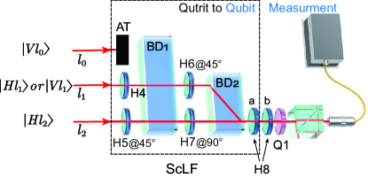
Figure 9: Experimental setups for performing the local filtering operation and the measurements of the filtered two-qubit states. The photons traveling through the upper optical path $|l_{0}\rangle$ are blocked via an absorbing termination (AT).

As mentioned above, our two-qutrit Werner state is encoded in the spatial DOF, decoupled from its polarization DOF, so the photonic polarization state could be changed at will by changing the setting of the HWPs H4 at both sides A and B. For definiteness, we make all the photons vertically polarized before the $\text{BD}_{1}$ in Fig. 9.

After the local filtering operation, the states change from a qutrit to a qubit, and we convert the encoding to polarization. With respect to Fig. 9, we see that for an arbitrary qutrit state

$$|\psi(\alpha,\beta,\gamma)\rangle:=\frac{\alpha|0\rangle+\beta|1\rangle+\gamma|2\rangle}{\sqrt{\alpha^{2}+\beta^{2}+\gamma^{2}}}$$ (10)

encoded in the spatial DOF of our setup, BD₁ and the HWP H6 transform $|\psi(\alpha,\beta,\gamma)\rangle$ as follows:

$$|\psi(\alpha,\beta,\gamma)\rangle\sim\frac{\alpha|Vl_{0}\rangle+\beta|H\text{ or }V\rangle|l_{1}\rangle+\gamma|Hl_{2}\rangle}{\sqrt{\alpha^{2}+\beta^{2}+\gamma^{2}}}$$ (11)

$$\xrightarrow[\text{photon on path}~{}l_{0}]{\text{block}}\frac{\beta|H\text{ or }V\rangle|l_{1}\rangle+\gamma|Hl_{2}\rangle}{\sqrt{\beta^{2}+\gamma^{2}}}$$

$$\xrightarrow[\text{photon on path}~{}l_{1}]{\text{H4}}\frac{\beta|Vl_{1}\rangle+\gamma|Hl_{2}\rangle}{\sqrt{\beta^{2}+\gamma^{2}}}$$

$$\xrightarrow[\text{photon on path}~{}l_{2}]{\text{H5}@45^{\circ}}\frac{\beta|Vl_{1}\rangle+\gamma|Vl_{2}\rangle}{\sqrt{\beta^{2}+\gamma^{2}}}$$

$$\xrightarrow[\text{photon on path}~{}l_{1},l_{2}]{\text{BD}_{1}}\frac{\beta|Vl_{1}\rangle+\gamma|Vl_{2}\rangle}{\sqrt{\beta^{2}+\gamma^{2}}}$$

$$\xrightarrow[\text{H7}@90^{\circ}\text{on }l_{2}]{\text{H6}@45^{\circ}\text{on }l_{1}}\frac{\beta|Hl_{1}\rangle+\gamma|Vl_{2}\rangle}{\sqrt{\beta^{2}+\gamma^{2}}}$$

$$\xrightarrow[\text{photon on path}~{}l_{1},l_{2}]{\text{BD}_{2}}\frac{\left(\beta|H\rangle+\gamma|V\rangle\right)|l_{2}\rangle}{\sqrt{\beta^{2}+\gamma^{2}}}\sim|\psi(\beta,\gamma)\rangle$$

By encoding $|H\rangle\to|1\rangle$ and $|V\rangle\to|2\rangle$, we obtain the qubit state

$$|\psi(\beta,\gamma)\rangle:=\frac{\beta|1\rangle+\gamma|2\rangle}{\sqrt{\beta^{2}+\gamma^{2}}},$$ (12)

which means that the qubit filtering operation is performed successfully. Note that these local operations already suffice for our experimental demonstration of single-copy distillation of quantum features. However, in the experiment, we have followed Li et al. (2021) to apply, additionally, the qubit rotations $\sigma_{x}$ and $\sigma_{z}$, see Eq. 30, thereby leading to different local filtering operations on the two sides. The qubit rotations can be realized by a HWP (H8a). Immediately following the HWP (H8b), a QWP (Q1) and a PBS are used to perform qubit measurements, and the two consecutive HWPs can be simplified to a single one (H8).

A.5 Experimental realization of an arbitrary Werner state

Although the decomposition that we have provided in Eq. 2 suffices for our experimental demonstration, it is not valid for $v>\frac{d+1}{2d}$, which leads to a negative value of $q=1-\frac{2d}{d+1}v$. For completeness, we provide below an alternative two-qudit decomposition of $W^{(d)}(v)$ valid for all $v\in[0,1]$. Explicitly, we note that

$$W^{(d)}(q)=\frac{1}{n^{d}_{-}}\sum_{i<j}\xi^{i,j}(p,q),\qquad$$ (13a)

$$\xi^{i,j}(p,q)=q\xi_{2}^{i,j}+\left(1-q\right)\left[p\xi_{0}^{i,j}+\left(1-p\right)\xi_{1}^{i,j}\right]$$ (13b)

where $p=\frac{(d+1)(1-v)}{d+1-2v}$, $q=\frac{2v}{d+1}$, $\xi_{0}^{i,j}=\varrho_{0}^{i,j}=|\Psi^{-}_{i,j}\rangle\!\langle\Psi^{-}_{i,j}|$, $\xi_{1}^{i,j}=|\Psi^{+}_{i,j}\rangle\!\langle\Psi^{+}_{i,j}|$, $|\Psi^{\pm}_{i,j}\rangle=\frac{1}{\sqrt{2}}(|i,j\rangle\pm|j,i\rangle)$, $\xi_{2}^{i,j}=\varrho_{1}^{i,j}=\frac{|ii\rangle\!\langle ii|+|jj\rangle\!\langle jj|}{2}$. It is easy to verify that $p,q\in[0,1]$ for $v\in[0,1]$, so all the Werner states can be prepared as a uniform mixture of the two-qubit states $\xi^{i,j}(p,q)$ acting locally on the qubit subspace spanned by $|i\rangle$ and $|j\rangle$. Accordingly, we can use the following optical setup to prepare the Werner state $W^{(d)}(v)$.

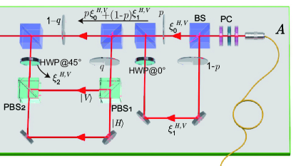
Figure 10: Experimental setup at A for realizing $\xi^{i,j}$ in Eq. 13, which requires slight modifications to be made in the part of Fig. 6.

Appendix B Miscellaneous Details and Theoretical Results

B.1 Bell-nonlocality

B.1.1 Symmetric (quasi-)extension

A powerful way to determine if a quantum state $\rho_{\text{AB}}$ could violate any Bell inequality is to check for the extent to which it admits a symmetric (quasi-)extension Doherty et al. (2002); Terhal et al. (2003). In particular, if $\rho_{\text{AB}}$ has a $(s_{a},1)$-symmetric (quasi-) extension, then it cannot violate any Bell inequality that has $s_{a}$ settings for Alice, and an arbitrary number of settings for Bob. A similar statement holds for a quantum state admitting a $(1,s_{b})$-symmetric (quasi-) extension.

For completeness (and simplicity of presentation), we provide below a semidefinite program (SDP) that facilitates the search for the existence of a $(k,1)$-symmetric extension Doherty et al. (2002) for any given $\rho_{\text{AB}}$ acting on $\mathbb{C}^{d_{A}}\otimes\mathbb{C}^{d_{B}}$. For the rest of this subsection, we shall refer to any $\rho_{\text{AB}}$ admitting a $(k,1)$-symmetric extension as being $k$-extendible. Our SDP formulation differs somewhat from of Doherty et al. (2002); Terhal et al. (2003) but makes explicit use of the two facts: (1) the set of $k$-extendible density matrices $\rho_{\text{AB}}$ is convex, and (2) the maximally mixed state $\frac{\mathbb{I}_{D}}{D}$, where $D:=d_{A}d_{B}$ is $k$-extendible for all $k>1$. Hence, if mixing $\rho_{\text{AB}}$ with a negatively-weighted $\frac{\mathbb{I}_{D}}{D}$ is $k$-extendible, $\rho_{\text{AB}}$ itself must already be $k$-extendible:

$$\ \ \min_{t\geq 0,\,\tilde{\rho}\succeq 0}\qquad\qquad\qquad\qquad t$$ (14)

$$\text{such that}\quad{\rm tr}_{\mathcal{H}^{\bar{\kappa}_{i}}}{\tilde{\rho}}=\rho_{\text{AB}}+(t-1)\frac{\mathbb{I}_{D}}{D},~{}\forall\,\,\kappa_{i}\in\{1,\dots,k\},$$

where $\bar{\kappa}_{i}=\{1,\dots,k\}\backslash\kappa_{i}$, i.e., the partial trace is over all but the $i$-th copy of $\mathbb{C}^{d_{A}}$ and $\succeq 0$ means matrix positivity. If the optimum value of this optimization is $t=t^{\star}\leq 1$, then $\tilde{\rho}+(1-t^{\star})\frac{\mathbb{I}_{d_{A}^{k}d_{B}}}{d_{A}^{k}d_{B}}$ is a legitimate quantum state that serves as the $(k,1)$-symmetric extension of $\rho_{\text{AB}}$.

Consider now $\rho_{\text{AB}}(w)$ decomposable as a convex mixture of an entangled state $\sigma$ and the maximally mixed state $\frac{\mathbb{I}_{D}}{D}$:

$$\rho_{\text{AB}}(w)=(1-w)\sigma+w\frac{\mathbb{I}_{D}}{D}.$$ (15)

Let $t^{\star}_{0}$ be the optimum value of $t$ obtained by solving Eq. 14 for $\sigma:=\rho_{\text{AB}}(w=0)$ and $w=w_{t}$ be the critical weight above which $\rho_{\text{AB}}(w)$ becomes $k$-extendible. By definition and the constraints of Eq. 14, we see that upon normalization,

$$\frac{1}{t^{\star}_{0}}\left[\sigma+(t^{\star}_{0}-1)\frac{\mathbb{I}_{D}}{D}\right]=\rho_{\text{AB}}\left(\frac{t^{\star}_{0}-1}{t^{\star}_{0}}\right)$$ (16)

must be $k$-extendible. In particular, all $\rho_{\text{AB}}(w)$ with $w<\frac{t^{\star}_{0}-1}{t^{\star}_{0}}$ is not $k$-extendible, or it would contradict the assumption that $t^{\star}_{0}$ is the optimum value obtained by solving Eq. 14 for $\rho_{\text{AB}}=\sigma$. Hence, $w_{t}=\frac{t^{\star}_{0}-1}{t^{\star}_{0}}$.

For Werner states $W^{(d)}(w)$, using the identity $\Pi^{d}_{+}=\mathbb{I}-\Pi^{d}_{-}$, we can also rewrite it from Eq. 1 as

$$W^{(d)}(v)=\left(1-\frac{Dv}{n^{d}_{+}}\right)\frac{\Pi^{d}_{-}}{n^{d}_{-}}+\frac{Dv}{n^{d}_{+}}\frac{\mathbb{I}}{D},$$ (17)

which is in the form of Eq. 15 if $\sigma=\frac{\Pi^{d}_{-}}{n^{d}_{-}}$, $w=\frac{Dv}{n^{d}_{+}}$, then

$$v_{t}=\frac{n^{d}_{+}}{D}w_{t}=\frac{n^{d}_{+}}{D}\frac{t^{\star}_{0}-1}{t^{\star}_{0}},$$ (18)

i.e., $W^{(d)}(v)$ for all $v>v_{t}$ is $k$-extendible.

To rule out the possibility of $\rho_{\text{AB}}$ violating any Bell inequality with a restricted number of settings, one can relax the SDP of Eq. 14 by considering an extension that is an entanglement witness, and hence not positive semidefinite. In particular, if we consider only a decomposable entanglement witness, then the following SDP facilitates the search for a symmetric $(k,1)$ quasi-extension of $\rho_{\text{AB}}$:

$$\ \ \min_{t\geq 0}\qquad\qquad\qquad\qquad t$$

$$\text{such that}\quad\tilde{H}_{\rho}=P+\sum_{p\in\mathcal{P}}Q^{\text{T}_{p}}_{p},$$

$$\qquad\qquad\ \ P\succeq 0,\quad Q_{p}\succeq 0~{}\forall\,\,p\in\mathcal{P}$$ (19)

$$\qquad\qquad\ \ {\rm tr}_{\mathcal{H}^{\bar{\kappa}_{i}}}{\tilde{H}_{p}}=\rho_{\text{AB}}+(t-1)\frac{\mathbb{I}_{D}}{D},~{}\forall\,\,\kappa_{i}\in\{1,\dots,k\},$$

where $\mathcal{P}$ is the set of all possible bipartitions. As with Eq. 14, if the optimum value of Section B.1.1 $t=t^{\star}\leq 1$, then $\tilde{H}_{p}+(1-t^{\star})\frac{\mathbb{I}_{d_{A}^{k}d_{B}}}{d_{A}^{k}d_{B}}$ serves as the $(k,1)$-symmetric quasiextension of $\rho_{\text{AB}}$.

In Table 2, we list our numerical results obtained by solving  Eq. 14 and Section B.1.1 for the Werner states $W^{(d)}(v)$. Note that due to limitations of computational resources, for determining the $(4,1)$-symmetric quasiextension, we only consider in $\mathcal{P}$ the following subset of bipartitions: $\{A_{1}|A_{2}A_{3}A_{4}B\},\{B|A_{1}A_{2}A_{3}A_{4}\},\{A_{1}A_{2}|A_{3}A_{4}B\}$, and $\{A_{1}B|A_{2}A_{3}A_{4}\}$, where $A_{k}$ denotes the $k$-copy of Alice’s subsystem. A similar simplification for the computation related to the $(1,4)$-symmetric quasiextension is adopted. Our findings suggest that in the case of Werner states $W^{(d)}(v)$, the relaxation from Eq. 14 to Section B.1.1 (with the simplification considered above) does not lead to the construction of a LHVM for a wider interval of entangled Werner states.

In Table 3, we also show, cf. Eq. 18, the threshold value of the symmetric weight above which the Werner states $W^{(d)}(v)$ admit a $(1,k)$ (bosonic Doherty (2014)) symmetric extension.

$(1,2)$	$\rho_{\text{expt}}(v)$		$W^{(3)}(v)$
$v$	SE	SQE	SE	SQE
$0$	1.0131	1.0086	1	1
$0.05$	1.0017	0.9876	0.9250	0.9250
$0.1$	1.0003	0.9886	0.8500	0.8500
$0.15$	0.9670	0.9369	0.7750	0.7750
$0.2$	0.9145	0.8469	0.7000	0.7000
$0.25$	0.7758	0.7022	0.6250	0.6250
$0.3$	0.7392	0.7004	0.5500	0.5500
$0.35$	0.5926	0.5505	0.4750	0.4750
$0.4$	0.6649	0.6161	0.4000	0.4000
$0.45$	0.4460	0.4062	0.3250	0.3250

$(1,3)$	$\rho_{\text{expt}}(v)$		$W^{(3)}(v)$
$v$	SE	SQE	SE	SQE
$0$	1.2725	1.2725	1.3333	1.3333
$0.05$	1.1813	1.1813	1.2333	1.2333
$0.1$	1.1630	1.1629	1.1333	1.1333
$0.15$	1.0939	1.0938	1.0333	1.0333
$0.2$	0.9912	0.9850	0.9333	0.9333
$0.25$	0.8387	0.8366	0.8333	0.8333
$0.3$	0.8083	0.8060	0.7333	0.7333
$0.35$	0.6359	0.6326	0.6333	0.6333
$0.4$	0.6668	0.6524	0.5333	0.5333
$0.45$	0.4593	0.4510	0.4333	0.4333

$(1,4)$	$\rho_{\text{expt}}(v)$		$W^{(3)}(v)$
$v$	SE	SQE	SE	SQE
$0$	1.5103	1.5098	1.6000	1.6000
$0.05$	1.3688	1.3685	1.4800	1.4800
$0.1$	1.3368	1.3363	1.3600	1.3600
$0.15$	1.2661	1.2659	1.2400	1.2400
$0.2$	1.1248	1.1222	1.1200	1.1200
$0.25$	0.9614	0.9610	1.0000	1.0000
$0.3$	0.9243	0.9225	0.8800	0.8800
$0.35$	0.7237	0.7221	0.7600	0.7600
$0.4$	0.7118	0.7111	0.6400	0.6400
$0.45$	0.5017	0.5004	0.5200	0.5200

$(2,1)$	$\rho_{\text{expt}}(v)$		$W^{(3)}(v)$
$v$	SE	SQE	SE	SQE
$0$	1.0196	1.0159	1	1
$0.05$	1.0000	0.9876	0.9250	0.9250
$0.1$	1.0000	0.9886	0.8500	0.8500
$0.15$	0.9670	0.9369	0.7750	0.7750
$0.2$	0.9145	0.8469	0.7000	0.7000
$0.25$	0.7758	0.7023	0.6250	0.6250
$0.3$	0.7392	0.7004	0.5500	0.5500
$0.35$	0.5926	0.5505	0.4750	0.4750
$0.4$	0.6649	0.6161	0.4000	0.4000
$0.45$	0.4460	0.4062	0.3250	0.3250

$(3,1)$	$\rho_{\text{expt}}(v)$		$W^{(3)}(v)$
$v$	SE	SQE	SE	SQE
$0$	1.2753	1.2753	1.3333	1.3333
$0.05$	1.1702	1.1700	1.2333	1.2333
$0.1$	1.1478	1.1472	1.1333	1.1333
$0.15$	1.0839	1.0830	1.0333	1.0333
$0.2$	0.9842	0.9787	0.9333	0.9333
$0.25$	0.8423	0.8401	0.8333	0.8333
$0.3$	0.8083	0.8063	0.7333	0.7333
$0.35$	0.6359	0.6319	0.6333	0.6333
$0.4$	0.6680	0.6553	0.5333	0.5333
$0.45$	0.4600	0.4508	0.4333	0.4333

$(4,1)$	$\rho_{\text{expt}}(v)$		$W^{(3)}(v)$
$v$	SE	SQE	SE	SQE
$0$	1.5097	1.5094	1.6000	1.6000
$0.05$	1.3660	1.3655	1.4800	1.4800
$0.1$	1.3321	1.3311	1.3600	1.3600
$0.15$	1.2633	1.2631	1.2400	1.2400
$0.2$	1.1237	1.1197	1.1200	1.1200
$0.25$	0.9628	0.9621	1.0000	1.0000
$0.3$	0.9223	0.9209	0.8800	0.8800
$0.35$	0.7217	0.7205	0.7600	0.7600
$0.4$	0.7139	0.7134	0.6400	0.6400
$0.45$	0.5012	0.5001	0.5200	0.5200

Table 2: Optimum results $t^{\star}$ obtained by solving Eq. 14 [Section B.1.1] for the existence of a $(k,1)$ or a $(1,k)$-symmetric (quasi-)extension, abbreviated as SE (SQE), for the ideal two-qutrit Werner state $W^{(3)}(v)$ and its experimental counterpart $\rho_{\text{expt}}(v)$. The state has a symmetric (quasi-)extension iff $t^{\star}\leq 1$. Due to limitations in the computational resource, in our computation of the symmetric quasi-extension for $k=4$ copies, only a subset of bipartitions is considered in the sum in Section B.1.1. See text for details. Since a Werner state is invariant under swapping Alice and Bob, i.e., $W^{(d)}(v)=VW^{(d)}(v)V^{\dagger}$, we see that $W^{(d)}(v)$ has a $(k,1)$ -symmetric (quasi-)extension iff it also has a $(1,k)$-symmetric (quasi-)extension. The experimentally prepared states $\rho_{\text{expt}}(v)$, however, are not exactly invariant under this permutation, resulting in slightly different values of $t^{\star}$ when solving for the symmetric (quasi-)extension with respect to the two parties.

	(1,2)		(1,3)		(1,4)		(1,5)		(1,6)		(1,7)		(1,8)		(1,9)		(1,10)		(1,11)		(1,12)		(1,13)
$d$	SE	SE-B	SE	SE-B	SE	SE-B	SE	SE-B	SE	SE-B	SE	SE-B	SE	SE-B	SE	SE-B	SE	SE-B	SE	SE-B	SE	SE-B	SE	SE-B
$2$	$\frac{1}{4}$	$\frac{1}{4}$	$\frac{1}{3}$	$\frac{1}{3}$	$\frac{3}{8}$	$\frac{3}{8}$	$\frac{2}{5}$	$\frac{2}{5}$	$\frac{5}{12}$	$\frac{5}{12}$	$\frac{3}{7}$	$\frac{3}{7}$		$\frac{7}{16}$		$\frac{4}{9}$		$\frac{9}{20}$		$\frac{5}{11}$		$\frac{11}{24}$		$\frac{6}{13}$
$3$	$0$	$\frac{1}{4}$	$\frac{1}{6}$	$\frac{1}{3}$	$\frac{1}{4}$	$\frac{3}{8}$		$\frac{2}{5}$		$\frac{5}{12}$		$\frac{3}{7}$		$\frac{7}{16}$
$4$	$0$	$\frac{1}{4}$	$0$	$\frac{1}{3}$		$\frac{3}{8}$		$\frac{2}{5}$		$\frac{5}{12}$
$5$	$0$	$\frac{1}{4}$		$\frac{1}{3}$		$\frac{3}{8}$
$6$	$0$	$\frac{1}{4}$		$\frac{1}{3}$
$7$	$0$	$\frac{1}{4}$

Table 3: Threshold value of $v$, denoted by $v_{t}$, above which the $d$-dimensional Werner states $W^{(d)}(v)$ are found to admit a $(1,k)$ symmetric extension (SE) or a $(1,k)$ bosonic symmetric extension (SE-B) Doherty (2014). The latter is a special kind of SE where the extension $\tilde{\rho}$ is further required to reside in the symmetric subspace of the $k$ copies of Alice. Being more constraining, the existence of a SE-B represents a tighter separability criterion compared with the existence of a SE. That is, for any given $d$ and $k$, the value of $v_{t}$ for SE-B is larger than or equal to that for SE. The values of $v_{t}$ presented in this Table may be related to the values of $t^{\star}$ presented in Table 2 for $W^{(d)}(v=0)$ via Eq. 18. Numerically, a $(1,k)$ extension is found until $v\simeq v_{t}-10^{-4}$. Blank entries correspond to those situations where we could not solve the SDP of Eq. 14 using the computation resources available. The value of $v_{t}=v_{\text{Sym}}:=\frac{1}{2}(1-\frac{d-1}{k})$ corresponding to the $(1,k)$ SE of $W^{(d)}(v)$ has been determined independently and analytically in Johnson and Viola (2013) (see also Terhal et al. (2003)). Interestingly, our results determined using the QETLAB toolbox Johnston (2016) suggests that $W^{(d)}(v)$ has a $(1,k)$ SE-B whenever $v\geq\frac{1}{2}\left(1-\frac{1}{k}\right)=\left.v_{\text{Sym}}\right|_{d=2}\geq v_{\text{Sym}}$, i.e., a $(1,k)$ SE-B for $W^{(d)}(v)$ exists for all $d>2$ iff a SE for $W^{(d=2)}(v)$ exists.

B.1.2 Finding Bell-nonlocal correlations for the experimentally produced two-qutrit states

For any given quantum correlation $\vec{P}_{\mathcal{Q}}$ attained by performing the local measurements described by the positive-operator-valued measures (POVMs) $\{M^{A}_{a|x}\}_{a,x}$ and $\{M^{B}_{b|y}\}_{b,y}$ on a shared density matrix $\rho_{\text{AB}}$:

$$P_{\mathcal{Q}}(a,b|x,y)={\rm tr}(\rho_{\text{AB}}\,M^{A}_{a|x}\otimes M^{B}_{b|y}),$$ (20)

we can determine if it is Bell-local by determining its nonlocal content Elitzur et al. (1992):

$$\min_{v\in[0,1],\vec{P}\in\mathcal{L},\vec{P}_{\text{NS}}}\qquad\quad v$$ (21a)

$$\text{such that \ \ }(1-v)\vec{P}+v\vec{P}_{\text{NS}}=\vec{P}_{\mathcal{Q}}$$ (21b)

where $\vec{P}_{\text{NS}}$ is any non-signaling correlation and $\mathcal{L}$ is the set of Bell-local correlations. If the result of this optimization is larger than $0$, we can conclude that $\vec{P}_{\mathcal{Q}}\not\in\mathcal{L}$ and hence $\vec{P}$ is Bell-nonlocal.

Since all $\rho_{\text{expt}}(v)$ with $v=0.01,\ldots,0.45$ admit a 2-symmetric quasiextension, it is necessary to consider a Bell scenario with at least $n_{s}=3$ measurement settings per site to identify its potential Bell-nonlocality. Moreover, given that these are two-qutrit states, it seems natural to consider Bell scenarios involving $n_{o}=3$ outcomes. To this end, our numerical maximizations using $\rho_{\text{expt}}(v)$ and the LB (see-saw) algorithm explained in Liang and Doherty (2007) have not led to any violation of the $21,169$ classes of facet-defining Bell inequalities from Cope and Colbeck (2019). In addition, we perform around $30,000$ double optimizations over the local measurements $\{M^{A}_{a|x}\}_{a,x}$ and $\{M^{B}_{b|y}\}_{b,y}$ to maximize the nonlocal content associated with these $\rho_{\text{expt}}(v)$ (including the one for $v=0$) for the $(n_{s},n_{o})=(3,3)$ Bell scenario and several thousand optimizations for the $(n_{s},n_{o})=(4,3)$. In all these cases, we have not found a single instance of $\vec{P}_{\mathcal{Q}}$ where the corresponding nonlocal content $v$ is unmistakably larger than zero.

B.2 Steering robustness

When Alice performs local measurements $\{M^{A}_{a|x}\}_{a,x}$ on the shared state $\rho_{\text{AB}}$, quantum theory dictates that, up to normalization, the conditional state prepared at Bob’s side is:

$$\rho_{a|x}={\rm tr}_{A}\left[{(M^{A}_{a|x}\otimes\mathbb{I})\rho_{\text{AB}}}\right].$$ (22)

In the studies of quantum steering Uola et al. (2020), the collection of these subnormalized conditional density matrices $\{\rho_{a|x}\}_{a,x}$ is called an assemblage. Accordingly, the extent to which Alice’s measurements can steer this assemblage can be quantified using the so-called steering robustness SR Piani and Watrous (2015), defined as the minimum value of $t$ such that $\{\frac{\rho_{a|x}+t\tau_{a|x}}{1+t}\}_{a,x}$ is unsteerable (admitting a local-hidden-state model) where $\{\tau_{a|x}\}_{a,x}$ is a valid assemblage.

For a given assemblage $\{\rho_{a|x}\}_{a,x}$, the corresponding SR can also be computed by solving the following SDP Cavalcanti and Skrzypczyk (2017):

$$\begin{split}\min_{\{\sigma_{\lambda}\}}&\quad\left(\sum_{\lambda}{\rm tr}\,\sigma_{\lambda}\right)-1\\ \text{s.t.}&\quad\sum_{\lambda}D(a|x,\lambda)\sigma_{\lambda}\succeq\rho_{a|x}~{}\forall a,x\\ &\quad\sigma_{\lambda}\succeq 0~{}\forall\,\,\lambda,\end{split}$$ (23)

where $D(a|x,\lambda)=\delta_{a,\lambda_{x}}$ are deterministic response functions and $\lambda=(\lambda_{1},\dots,\lambda_{n_{s}})$.

To quantify the steerability of a quantum state $\rho_{\text{AB}}$ from A to B, one can optimize SR over all possible measurement strategies of Alice, i.e.,

$$\text{SR}_{A\to B}\left(\rho_{\text{AB}}\right):= \max_{\{M^{A}_{a|x}\}_{a,x}}\quad\text{SR}\left(\{\rho_{a|x}\}_{a,x}\right)$$ (24)

$$\text{s.t.}\quad\rho_{a|x}={\rm tr}_{A}\left[{(M^{A}_{a|x}\otimes\mathbb{I})\rho_{\text{AB}}}\right]~{}\forall\,\,a,x.$$

Evidently, a similar definition can be given for $\text{SR}_{B\to A}\left(\rho_{\text{AB}}\right)$. Then, following Chen et al. (2016), we can define

$$\text{SR}\left(\rho_{\text{AB}}\right):=\max\{\text{SR}_{A\to B}\left(\rho_{\text{AB}}\right),\text{SR}_{B\to A}\left(\rho_{\text{AB}}\right)\}.$$ (25)

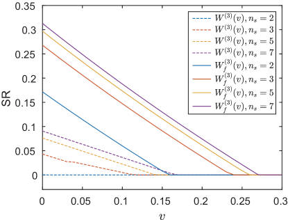
Figure 11: Best lower bounds on the steering robustness SR found for $W^{(3)}(v)$ (dashed lines) and $W^{(3)}_{f}(v)$ (solid lines) for various number $n_{s}$ of measurement settings and $v=0,0.01,\cdots,0.3$.

For $W^{(d)}(v)$ and $W^{(d)}_{f}(v)$, both invariant with respect to swapping $A$ and $B$, we have $\text{SR}\left(\rho_{\text{AB}}\right)=\text{SR}_{A\to B}\left(\rho_{\text{AB}}\right)$. In principle, there is no limitation to the number of measurement settings $n_{s}$ and the number of outcomes $n_{o}$ in Eq. 24. In Fig. 11, we provide the best lower bounds on SR for $W^{(3)}(v)$ and $W^{(3)}_{f}(v)$ we have found by considering up to $n_{s}=7$. For each of them, we set $n_{o}=d$, the local Hilbert space dimension, and obtain these results using the optimization code of Cavalcanti and Skrzypczyk (2017) by considering $1,000$ random initial local measurements $\{M^{A}_{a|x}\}_{a,x}$. It is worth noting from Fig. 11 that with only $n_{s}=2$ measurement settings, it appears impossible to demonstrate the steerability of $W^{(3)}(v)$.

B.3 Dense-codability

The Holevo bound Nielsen and Chuang (2011) says that the amount of classical information that can be transmitted using a $d$-dimensional quantum state is at most $\log_{2}(d)$ bits. However, with shared entanglement, it is possible to go beyond this bound through a dense coding protocol Bennett and Wiesner (1992). To this end, let Alice and Bob share a two-qudit state $\rho_{\text{AB}}$. Suppose Alice applies a local unitary $U_{i}$ with probability $p_{i}$ on her qudit and sends it to Bob. This means that she effectively prepares an ensemble $\{p_{i},\rho_{\text{AB},i}\}$ for Bob. Upon receiving the qudit, Bob tries to decode the index $i$ by performing a joint measurement on $(U_{i}\otimes\mathbb{I}_{B})\rho_{\text{AB}}(U_{i}\otimes\mathbb{I}_{B})^{\dagger}$.

By using an optimal choice of orthogonal unitaries, Ref. Bruß et al. (2004) shows that the dense coding capacity $\chi$ (in bits) of a two-qudit state $\rho_{\text{AB}}$ with Alice sending her qudit to Bob is quantified by $\chi(\rho_{\text{AB}}):=\log_{2}d+S(\rho_{\text{B}})-S(\rho_{\text{AB}})$, where $S(\cdot)$ denotes the von Neumann entropy Nielsen and Chuang (2011). Compared with the Holevo bound $\log_{2}d$, one finds that a quantum state is useful for dense coding from A to B if

$$\delta(\rho_{\text{AB}}):=S(\rho_{\text{B}})-S(\rho_{\text{AB}})>0.$$ (26)

For the two-qudit Werner states $W^{(d)}(v)$, we have

$$\delta[W^{(d)}(v)]= \log_{2}d+v\log_{2}\frac{2v}{d(d+1)}$$ (27)

$$+(1-v)\log_{2}\frac{2(1-v)}{d(d-1)},$$

which is easily verified to be negative for all $d\geq 3$ and $v\in[0,1]$. Thus, all $W^{(d)}(v)$ for $d\geq 3$ are useless for dense coding.

However, upon qubit filtering operation, $W^{(d)}(v)$ becomes $W^{(d)}_{f}(v)$, which is local-unitarily equivalent to $W^{(2)}(v^{\prime})$ with $v^{\prime}=\frac{3(d-1)v}{N_{d,v}}$ where $N_{d,v}:=(d+1)(1-v)+3v(d-1)$. Using this in Eq. 27 with $d=2$, we obtain

$$\delta[W^{(d)}_{f}(v)]= ~{}1+\frac{(d+1)(1-v)}{N_{d,v}}\log_{2}\frac{(d+1)(1-v)}{N_{d,v}}$$

$$+\frac{3v(d-1)}{N_{d,v}}\log_{2}\frac{v(d-1)}{N_{d,v}}.$$ (28)

Numerically, we can solve the critical value of $v$, denoted by $v_{dc}$ below which $\delta[W^{(d)}_{f}(v)]$ becomes larger than zero. The corresponding results for $d=2,3,\cdots,16$ are shown in Fig. 12. In the asymptotic limit of $d\to\infty$, our computation suggests that $v_{dc}$ approaches $\sim 0.0722088$.

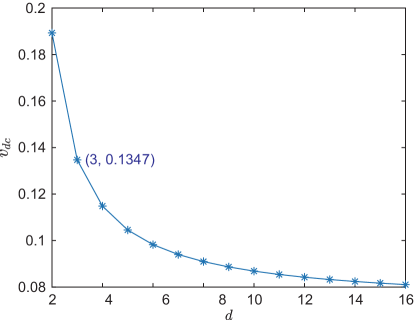
Figure 12: Threshold value of $v$ below which Section B.3 becomes larger than zero, i.e., where $W^{(d)}(v)$ may be locally filtered by qubit projection to become useful for dense coding.

Appendix C Other experimental results and analysis

Here, we provide other relevant experimental results omitted from the main text, including the reconstructed density matrices, their fidelity with respect to the reference state, the steering robustness, and the dense codability of the filtered quantum states.

C.1 Experimental states and fidelity

From the definition of $W^{(d)}(v)$ given in Eq. 1 and the explicit form of the swap operator:

$$V=\sum_{i,j}(|i\rangle\!\langle j|)_{A}\otimes(|j\rangle\!\langle i|)_{B},$$ (29)

we see that in the computational basis $\{|i\rangle\}_{i=0}^{d-1}$, Werner states $W^{(d)}(v)$ may be represented by a density matrix using only real matrix elements, likewise for the filtered two-qubit density operator $W^{(d)}_{f}(v)$, and the rotated version Li et al. (2021) prepared in our experiment:

$$\widetilde{W}^{(3)}_{f}(v) =(\sigma_{x}\otimes\sigma_{z})W^{(3)}_{f}(v)(\sigma_{x}\otimes\sigma_{z})^{\dagger},$$ (30)

$$=\frac{1}{N_{3,v}}\left[4(1-v)|\Phi^{+}_{2}\rangle\!\langle\Phi^{+}_{2}|+2v(\mathbb{I}_{4}-|\Phi^{+}_{2}\rangle\!\langle\Phi^{+}_{2}|)\right],$$

where $N_{3,v}=4(1-v)+6v$ and $|\Phi^{+}_{2}\rangle=\frac{1}{\sqrt{2}}(|1\rangle|2\rangle+|2\rangle|1\rangle)$. As an illustration of the quality of the experimentally prepared states, we show in Fig. 13 the real part of the unfiltered and filtered states prepared in the experiment.

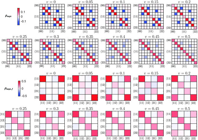
Figure 13: Experimentally (reconstructed) density matrix of the unfiltered states $\rho_{\text{expt}}(v)$ and the filtered states $\rho_{{\text{expt}},f}(v)$.

It is also conventional to use a fidelity measure Liang et al. (2019) to quantify the quality of the experimentally prepared state with respect to the target state. In particular, a widely adopted choice for quantifying the similarity between two density matrices $\rho$ and $\sigma$ is given by the Uhlmann-Jozsa fidelity:

$$F(\rho,\sigma)=\left[{\rm tr}\sqrt{\sqrt{\rho}\sigma\sqrt{\rho}}\right]^{2}=F(\sigma,\rho).$$ (31)

Accordingly, we show in Table 4 the fidelity of the experimentally prepared two-qutrit states $\rho_{\text{expt}}(v)$ and their filtered two-qubit counterparts $\rho_{\text{expt},f}(v)$ with respect to, respectively, $W^{(3)}(v)$ and $\widetilde{W}^{(3)}_{f}(v)$.

Table 4: Fidelity between the experimentally prepared states $\rho_{\text{expt}}(v)$ [$\rho_{\text{expt},f}(v)$] and their theory counterparts $W^{(3)}(v)$ [$\widetilde{W}^{(3)}_{f}(v)$].

$v$	$F[\rho_{\text{expt}}(v),W^{(d)}(v)]$	$F[\rho_{\text{expt},f}(v),\widetilde{W}^{(3)}_{f}(v)]$
$0$	$0.958\pm 0.002$	$0.934\pm 0.006$
$0.05$	$0.965\pm 0.001$	$0.948\pm 0.001$
$0.1$	$0.963\pm 0.001$	$0.965\pm 0.003$
$0.15$	$0.981\pm 0.005$	$0.974\pm 0.003$
$0.2$	$0.982\pm 0.004$	$0.985\pm 0.002$
$0.25$	$0.990\pm 0.001$	$0.975\pm 0.002$
$0.3$	$0.991\pm 0.001$	$0.990\pm 0.001$
$0.35$	$0.995\pm 0.001$	$0.992\pm 0.001$
$0.4$	$0.980\pm 0.003$	$0.995\pm 0.001$
$0.45$	$0.993\pm 0.001$	$0.995\pm 0.001$
$0.5$	$0.994\pm 0.001$	$0.994\pm 0.001$

C.2 Steering robustness

For completeness, we provide here, in comparison with Fig. 11, our best lower bounds on the steering robustness of the experimentally prepared states utilizing up to $n_{s}=7$ measurement bases. Notice that due to the asymmetry in the experimentally produced states, Eq. 24 no longer coincides with Eq. 25. Consequently, our results for SR_A→B shown in Fig. 11, even though they still serve as a legitimate lower bound, may not represent the tightest lower bound on SR. Nonetheless, it is clear from Fig. 11 that for any given $n_{s}$ and a non-vanishing interval of $v$, we see an improvement in these lower bounds on SR after the implemented ScLF.

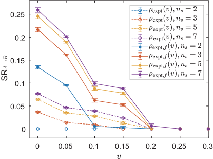
Figure 14: Best lower bounds on the steering robustness $\text{SR}_{A\to B}$ found for $\rho_{\text{expt}}(v)$ (hollow markers) and $\rho_{\text{expt},f}(v)$ (filled markers) for various number of Alice’s measurement settings $n_{s}$. The lines are guides for the eye.

C.3 Dense-codability

Similarly, we provide in Fig. 15, for completeness, a plot of the dense-codability of the experimentally prepared states before and after the ScLF. Again, the results clearly demonstrate the activation of dense codability for $v=0$ and $0.05$. However, the expected activation for $v=0.10$ is not observed in our imperfect experimental implementation.

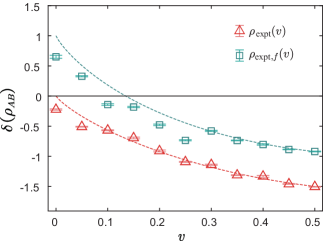
Figure 15: A bipartite quantum state $\rho_{\text{AB}}$ is useful for dense coding Bruß et al. (2004) if the quantity $\delta(\rho_{\text{AB}}):=S(\rho_{\text{B}})-S(\rho_{\text{AB}})>0$. Triangular (red) and square (green) markers show, respectively, $\delta[\rho_{\text{expt}}(v)]$ and $\delta[\rho_{\text{expt},f}(v)]$. Accordingly, the lower and upper dashed lines show $\delta[W^{(d)}(v)]$ and $\delta[W^{(d)}_{f}(v)]$.

References

- Horodecki et al. (2009) R. Horodecki, P. Horodecki, M. Horodecki, and K. Horodecki, Rev. Mod. Phys. 81, 865 (2009).
- Bell (1964) J. S. Bell, Physics 1, 195 (1964).
- Jozsa and Linden (2003) R. Jozsa and N. Linden, Proc. R. Soc. A 459, 2011 (2003).
- Vidal (2003) G. Vidal, Phys. Rev. Lett. 91, 147902 (2003).
- Ekert (1991) A. K. Ekert, Phys. Rev. Lett. 67, 661 (1991).
- Bennett and Wiesner (1992) C. H. Bennett and S. J. Wiesner, Phys. Rev. Lett. 69, 2881 (1992).
- Tóth and Apellaniz (2014) G. Tóth and I. Apellaniz, J. Phys. A 47, 424006 (2014).
- Wehner et al. (2018) S. Wehner, D. Elkouss, and R. Hanson, Science 362, eaam9288 (2018).
- Żukowski et al. (1993) M. Żukowski, A. Zeilinger, M. A. Horne, and A. K. Ekert, Phys. Rev. Lett. 71, 4287 (1993).
- Yin et al. (2017) J. Yin, Y. Cao, Y.-H. Li, S.-K. Liao, L. Zhang, J.-G. Ren, W.-Q. Cai, W.-Y. Liu, B. Li, H. Dai, G.-B. Li, Q.-M. Lu, Y.-H. Gong, Y. Xu, S.-L. Li, F.-Z. Li, Y.-Y. Yin, Z.-Q. Jiang, M. Li, J.-J. Jia, G. Ren, D. He, Y.-L. Zhou, X.-X. Zhang, N. Wang, X. Chang, Z.-C. Zhu, N.-L. Liu, Y.-A. Chen, C.-Y. Lu, R. Shu, C.-Z. Peng, J.-Y. Wang, and J.-W. Pan, Science 356, 1140 (2017).
- Bennett et al. (1996) C. H. Bennett, G. Brassard, S. Popescu, B. Schumacher, J. A. Smolin, and W. K. Wootters, Phys. Rev. Lett. 76, 722 (1996).
- Deutsch et al. (1996) D. Deutsch, A. Ekert, R. Jozsa, C. Macchiavello, S. Popescu, and A. Sanpera, Phys. Rev. Lett. 77, 2818 (1996).
- Horodecki and Horodecki (1999) M. Horodecki and P. Horodecki, Phys. Rev. A 59, 4206 (1999).
- Gisin (1996) N. Gisin, Phys. Lett. A 210, 151 (1996).
- Peres (1996) A. Peres, Phys. Rev. Lett. 77, 1413 (1996).
- Horodecki et al. (1998) M. Horodecki, P. Horodecki, and R. Horodecki, Phys. Rev. Lett. 80, 5239 (1998).
- DiVincenzo et al. (2000) D. P. DiVincenzo, P. W. Shor, J. A. Smolin, B. M. Terhal, and A. V. Thapliyal, Phys. Rev. A 61, 062312 (2000).
- Dür et al. (2000) W. Dür, J. I. Cirac, M. Lewenstein, and D. Bruß, Phys. Rev. A 61, 062313 (2000).
- Werner (1989) R. F. Werner, Phys. Rev. A 40, 4277 (1989).
- Horodecki et al. (1997) M. Horodecki, P. Horodecki, and R. Horodecki, Phys. Rev. Lett. 78, 574 (1997).
- Steinlechner et al. (2017) F. Steinlechner, S. Ecker, M. Fink, B. Liu, J. Bavaresco, M. Huber, T. Scheidl, and R. Ursin, Nat. Commun. 8, 15971 (2017).
- Ecker et al. (2019) S. Ecker, F. Bouchard, L. Bulla, F. Brandt, O. Kohout, F. Steinlechner, R. Fickler, M. Malik, Y. Guryanova, R. Ursin, and M. Huber, Phys. Rev. X 9, 041042 (2019).
- Hu et al. (2020a) X.-M. Hu, W.-B. Xing, B.-H. Liu, D.-Y. He, H. Cao, Y. Guo, C. Zhang, H. Zhang, Y.-F. Huang, C.-F. Li, and G.-C. Guo, Optica 7, 738 (2020a).
- Liu et al. (2002) X. S. Liu, G. L. Long, D. M. Tong, and F. Li, Phys. Rev. A 65, 022304 (2002).
- Liang et al. (2003) Y. C. Liang, D. Kaszlikowski, B.-G. Englert, L. C. Kwek, and C. H. Oh, Phys. Rev. A 68, 022324 (2003).
- Vértesi et al. (2010) T. Vértesi, S. Pironio, and N. Brunner, Phys. Rev. Lett. 104, 060401 (2010).
- Horodecki et al. (2022) P. Horodecki, L. Rudnicki, and K. Życzkowski, PRX Quantum 3, 010101 (2022).
- Watrous (2004) J. Watrous, Phys. Rev. Lett. 93, 010502 (2004).
- Fang and Liu (2020) K. Fang and Z.-W. Liu, Phys. Rev. Lett. 125, 060405 (2020).
- Fang and Liu (2022) K. Fang and Z.-W. Liu, PRX Quantum 3, 010337 (2022).
- Regula (2022) B. Regula, Phys. Rev. Lett. 128, 110505 (2022).
- Horodecki et al. (1999) M. Horodecki, P. Horodecki, and R. Horodecki, Phys. Rev. A 60, 1888 (1999).
- Popescu (1994) S. Popescu, Phys. Rev. Lett. 72, 797 (1994).
- Pan et al. (2001) J.-W. Pan, C. Simon, Č. Brukner, and A. Zeilinger, Nature 410, 1067 (2001).
- Pan et al. (2003) J.-W. Pan, S. Gasparoni, R. Ursin, G. Weihs, and A. Zeilinger, Nature 423, 417 (2003).
- Zhao et al. (2003) Z. Zhao, T. Yang, Y.-A. Chen, A.-N. Zhang, and J.-W. Pan, Phys. Rev. Lett. 90, 207901 (2003).
- Yamamoto et al. (2003) T. Yamamoto, M. Koashi, Ş. K. Özdemir, and N. Imoto, Nature 421, 343 (2003).
- Walther et al. (2005) P. Walther, K. J. Resch, Č. Brukner, A. M. Steinberg, J.-W. Pan, and A. Zeilinger, Phys. Rev. Lett. 94, 040504 (2005).
- Reichle et al. (2006) R. Reichle, D. Leibfried, E. Knill, J. Britton, R. B. Blakestad, J. D. Jost, C. Langer, R. Ozeri, S. Seidelin, and D. J. Wineland, Nature 443, 838 (2006).
- Kalb et al. (2017) N. Kalb, A. A. Reiserer, P. C. Humphreys, J. J. W. Bakermans, S. J. Kamerling, N. H. Nickerson, S. C. Benjamin, D. J. Twitchen, M. Markham, and R. Hanson, Science 356, 928 (2017).
- Hu et al. (2021a) X.-M. Hu, C.-X. Huang, Y.-B. Sheng, L. Zhou, B.-H. Liu, Y. Guo, C. Zhang, W.-B. Xing, Y.-F. Huang, C.-F. Li, and G.-C. Guo, Phys. Rev. Lett. 126, 010503 (2021a).
- Ecker et al. (2021) S. Ecker, P. Sohr, L. Bulla, M. Huber, M. Bohmann, and R. Ursin, Phys. Rev. Lett. 127, 040506 (2021).
- Zhao et al. (2017) Y.-Y. Zhao, M. Grassl, B. Zeng, G.-Y. Xiang, C. Zhang, C.-F. Li, and G.-C. Guo, npj Quantum Inf. 3, 11 (2017).
- Singh et al. (2021) J. Singh, S. Ghosh, . Arvind, and S. K. Goyal, Phys. Lett. A 392, 127158 (2021).
- Pramanik et al. (2019) T. Pramanik, Y.-W. Cho, S.-W. Han, S.-Y. Lee, Y.-S. Kim, and S. Moon, Phys. Rev. A 99, 030101 (2019).
- Nery et al. (2020) R. V. Nery, M. M. Taddei, P. Sahium, S. P. Walborn, L. Aolita, and G. H. Aguilar, Phys. Rev. Lett. 124, 120402 (2020).
- Hao et al. (2024) Z.-Y. Hao, Y. Wang, J.-K. Li, Y. Xiang, Q.-Y. He, Z.-H. Liu, M. Yang, K. Sun, J.-S. Xu, C.-F. Li, and G.-C. Guo, Phys. Rev. A 109, 022411 (2024).
- Zhang et al. (2024) Q.-X. Zhang, X.-X. Fang, and H. Lu, Photonics Res. 12, 552 (2024).
- Wiseman et al. (2007) H. M. Wiseman, S. J. Jones, and A. C. Doherty, Phys. Rev. Lett. 98, 140402 (2007).
- Uola et al. (2020) R. Uola, A. C. S. Costa, H. C. Nguyen, and O. Gühne, Rev. Mod. Phys. 92, 015001 (2020).
- Li et al. (2021) J.-Y. Li, X.-X. Fang, T. Zhang, G. N. M. Tabia, H. Lu, and Y.-C. Liang, Phys. Rev. Research 3, 023045 (2021).
- Masanes (2006) L. Masanes, Phys. Rev. Lett. 96, 150501 (2006).
- Kwiat et al. (2001) P. G. Kwiat, S. Barraza-Lopez, A. Stefanov, and N. Gisin, Nature 409, 1014 (2001).
- Wang et al. (2006) Z.-W. Wang, X.-F. Zhou, Y.-F. Huang, Y.-S. Zhang, X.-F. Ren, and G.-C. Guo, Phys. Rev. Lett. 96, 220505 (2006).
- Wang et al. (2020) Y. Wang, J. Li, X.-R. Wang, T.-J. Liu, and Q. Wang, Opt. Express 28, 13638 (2020).
- Popescu (1995) S. Popescu, Phys. Rev. Lett. 74, 2619 (1995).
- Kumari (2024) A. Kumari, Phys. Scr 99, 085114 (2024).
- Masanes et al. (2008) L. Masanes, Y.-C. Liang, and A. C. Doherty, Phys. Rev. Lett. 100, 090403 (2008).
- Liang et al. (2012) Y.-C. Liang, L. Masanes, and D. Rosset, Phys. Rev. A 86, 052115 (2012).
- Thew et al. (2004) R. T. Thew, A. Acín, H. Zbinden, and N. Gisin, Phys. Rev. Lett. 93, 010503 (2004).
- Huber et al. (2010) M. Huber, F. Mintert, A. Gabriel, and B. C. Hiesmayr, Phys. Rev. Lett. 104, 210501 (2010).
- Schwarz et al. (2016) S. Schwarz, B. Bessire, A. Stefanov, and Y.-C. Liang, New J. Phys. 18, 035001 (2016).
- Martin et al. (2017) A. Martin, T. Guerreiro, A. Tiranov, S. Designolle, F. Fröwis, N. Brunner, M. Huber, and N. Gisin, Phys. Rev. Lett. 118, 110501 (2017).
- Islam et al. (2017) N. T. Islam, C. C. W. Lim, C. Cahall, J. Kim, and D. J. Gauthier, Sci. Adv. 3, e1701491 (2017).
- Bavaresco et al. (2018) J. Bavaresco, N. Herrera Valencia, C. Klöckl, M. Pivoluska, P. Erker, N. Friis, M. Malik, and M. Huber, Nature Physics 14, 1032 (2018).
- Zeng et al. (2018) Q. Zeng, B. Wang, P. Li, and X. Zhang, Phys. Rev. Lett. 120, 030401 (2018).
- Wang et al. (2018) J. Wang, S. Paesani, Y. Ding, R. Santagati, P. Skrzypczyk, A. Salavrakos, J. Tura, R. Augusiak, L. Mančinska, D. Bacco, D. Bonneau, J. W. Silverstone, Q. Gong, A. Acín, K. Rottwitt, L. K. Oxenløwe, J. L. O’Brien, A. Laing, and M. G. Thompson, Science 360, 285 (2018).
- Hu et al. (2018) X.-M. Hu, Y. Guo, B.-H. Liu, Y.-F. Huang, C.-F. Li, and G.-C. Guo, Sci. Adv. 4, eaat9304 (2018).
- Lu et al. (2020) L. Lu, L. Xia, Z. Chen, L. Chen, T. Yu, T. Tao, W. Ma, Y. Pan, X. Cai, Y. Lu, S. Zhu, and X.-S. Ma, npj Quantum Inf. 6, 30 (2020).
- Dada et al. (2011) A. C. Dada, J. Leach, G. S. Buller, M. J. Padgett, and E. Andersson, Nat. Phys. 7, 677 (2011).
- Hu et al. (2020b) X.-M. Hu, W.-B. Xing, B.-H. Liu, Y.-F. Huang, C.-F. Li, G.-C. Guo, P. Erker, and M. Huber, Phys. Rev. Lett. 125, 090503 (2020b).
- Hu et al. (2021b) X.-M. Hu, W.-B. Xing, Y. Guo, M. Weilenmann, E. A. Aguilar, X. Gao, B.-H. Liu, Y.-F. Huang, C.-F. Li, G.-C. Guo, Z. Wang, and M. Navascués, Phys. Rev. Lett. 127, 220501 (2021b).
- Designolle et al. (2021) S. Designolle, V. Srivastav, R. Uola, N. H. Valencia, W. McCutcheon, M. Malik, and N. Brunner, Phys. Rev. Lett. 126, 200404 (2021).
- Qu et al. (2022a) R. Qu, Y. Wang, X. Zhang, S. Ru, F. Wang, H. Gao, F. Li, and P. Zhang, Optica 9, 473 (2022a).
- Qu et al. (2022b) R. Qu, Y. Wang, M. An, F. Wang, Q. Quan, H. Li, H. Gao, F. Li, and P. Zhang, Phys. Rev. Lett. 128, 240402 (2022b).
- Horodecki and Horodecki (2001) P. Horodecki and R. Horodecki, Quant. Inf. Comput. 1, 45 (2001).
- Bruß et al. (2004) D. Bruß, G. M. D’Ariano, M. Lewenstein, C. Macchiavello, A. Sen(De), and U. Sen, Phys. Rev. Lett. 93, 210501 (2004).
- Clauser et al. (1969) J. F. Clauser, M. A. Horne, A. Shimony, and R. A. Holt, Phys. Rev. Lett. 23, 880 (1969).
- Johnson and Viola (2013) P. D. Johnson and L. Viola, Phys. Rev. A 88, 032323 (2013).
- Terhal et al. (2003) B. M. Terhal, A. C. Doherty, and D. Schwab, Phys. Rev. Lett. 90, 157903 (2003).
- Doherty et al. (2002) A. C. Doherty, P. A. Parrilo, and F. M. Spedalieri, Phys. Rev. Lett. 88, 187904 (2002).
- Doherty (2014) A. C. Doherty, J. Phys. A: Math. Theor. 47, 424004 (2014).
- Altepeter et al. (2005) J. Altepeter, E. Jeffrey, and P. Kwiat, in Advances In Atomic, Molecular, and Optical Physics, Vol. 52 (Elsevier, 2005) pp. 105–159.
- Gurvits and Barnum (2002) L. Gurvits and H. Barnum, Phys. Rev. A 66, 062311 (2002).
- Horodecki et al. (1995) R. Horodecki, P. Horodecki, and M. Horodecki, Phys. Lett. A 200, 340 (1995).
- Horodecki et al. (1996) R. Horodecki, M. Horodecki, and P. Horodecki, Phys. Lett. A 222, 21 (1996).
- Piani and Watrous (2015) M. Piani and J. Watrous, Phys. Rev. Lett. 114, 060404 (2015).
- Cavalcanti and Skrzypczyk (2017) D. Cavalcanti and P. Skrzypczyk, Rep. Prog. Phys. 80, 024001 (2017).
- Chen et al. (2016) S.-L. Chen, C. Budroni, Y.-C. Liang, and Y.-N. Chen, Phys. Rev. Lett. 116, 240401 (2016).
- Johnston (2016) N. Johnston, “QETLAB: A MATLAB toolbox for quantum entanglement, version 0.9,” https://qetlab.com (2016).
- Elitzur et al. (1992) A. C. Elitzur, S. Popescu, and D. Rohrlich, Phys. Lett. A 162, 25 (1992).
- Liang and Doherty (2007) Y.-C. Liang and A. C. Doherty, Phys. Rev. A 75, 042103 (2007).
- Cope and Colbeck (2019) T. Cope and R. Colbeck, Phys. Rev. A 100, 022114 (2019).
- Nielsen and Chuang (2011) M. A. Nielsen and I. L. Chuang, Quantum Computation and Quantum Information (Cambridge ; New York : Cambridge University Press, 2011).
- Liang et al. (2019) Y.-C. Liang, Y.-H. Yeh, P. E. M. F. Mendonça, R. Y. Teh, M. D. Reid, and P. D. Drummond, Rep. Prog. Phys. 82, 076001 (2019).