Towards optimal algorithms for the recovery of low-dimensional models with linear rates

Abstract

We consider the problem of recovering elements of a low-dimensional model from linear measurements. From signal and image processing to inverse problems in data science, this question has been at the center of many applications. Lately, with the success of models and methods relying on deep neural networks leading to non-convex formulations, traditional convex variational approaches have shown their limits. Furthermore, the multiplication of algorithms and recovery results makes identifying the best methods a complex task. In this article, we study recovery with a class of widely used algorithms without considering any underlying functional. This result leads to a class of projected gradient descent algorithms that recover a given low-dimensional with linear rates. The obtained rates decouple the impact of the quality of the measurements with respect to the model from its intrinsic complexity. As a consequence, we can directly measure the performance of this class of projected gradient descents through a restricted Lipschitz constant of the projection. By optimizing this constant, we define optimal algorithms. Our general approach provides an optimality result in the case of sparse recovery. Moreover, we uncover underlying linear rates of convergence for some “plug and play” imaging methods relying on deep priors by interpreting our results in this context, thus linking low-dimensional recovery and recovery with deep priors under a unified theory, validated by experiments on synthetic and real data.

1 Introduction

In this paper, we consider the general noiseless observation model in finite dimension:

$$y=A\hat{x}$$ (1)

where $y$ is an $m$-dimensional vector of measurements, $A$ is an under-determined linear operator from $\mathbb{R}^{N}$ to $\mathbb{C}^{m}$ (i.e. $m<n$) and $\hat{x}\in\mathbb{R}^{N}$ is the unknown vector we want to recover. The problem of recovering $\hat{x}$ from $y$ is ill-posed. It is thus necessary to use prior information on $\hat{x}$ to hope for an estimation of $\hat{x}$ with a guarantee of success.

In this work, we suppose that $\hat{x}$ belongs to a (potentially infinite) union of subspaces $\Sigma$ (i.e. a homogeneous set: for every $x\in\Sigma$ and $\lambda\in\mathbb{R}$, $\lambda x\in\Sigma$) that models known properties of the unknown. Examples of such models include sparse as well as low-rank models and many of their generalizations (see [14] for an overview). The problem of recovering elements of a low-dimensional model from their measurements has been at the center of inverse problems in data science. This is for instance the case for many problems in signal and image processing where the unknown $\hat{x}$ is the signal or image of interest, and the matrix $A$ models a degradation such as a subsampling or a blur. Note that, in this article, we consider the noiseless case as we focus on the geometry of the estimation of elements of $\Sigma$ in relation to the chosen algorithm and the measurement operator $A$.

To recover $\hat{x}$, a classical method is to solve the minimization problem

$$x^{\star}\in\arg\min\frac{1}{2}\|Ax-y\|_{2}^{2}+\lambda R(x)$$ (2)

where $R$ is a function – the regularizer – that enforces some structure on the solution $x^{\star}$. Without any assumption on the easiness of the calculation of $x^{\star}$, functions $R$ of the form $d(\cdot,\Sigma)$ (distance to the model set for a given norm) achieve the best identifiability guarantees [7]. Unfortunately, for classical low-dimensional models such as sparse models such minimization is NP hard [20].

Another possibility is to use a convex proxy of minimization (2) (i.e. using a convex $R$) that guarantees the recovery of elements of $\Sigma$. A general method for the best possible choice of convex regularization $R$ has been presented in [37]. However, in terms of practical recovery guarantees, one must combine guarantees of success of (2) with convergence guarantees of the chosen algorithm.

While the convergence of many algorithms is verified for any instance of the convex problems, for the non-convex methods, heuristics approximating the minimization of (2) are studied directly, and identifiability guarantees of the chosen algorithm are proven under conditions much more stringent than the guarantees of the ideal non-convex minimization. Moreover, it is often hard to compare results accurately with convex methods, resulting in potentially different behaviors between theoretical results and practical implementations of said methods.

In this landscape of methods for solving inverse problems, algorithms based on deep priors have become the state-of-the-art reference in domains such as image processing. These methods have in common the fact that the prior used, one way or another, is learned on a large database with a deep neural network (DNN). Such priors are called deep priors. A large part of the resulting algorithms, such as plug-and-play methods (PnP) [39] fall within a non-convex framework, which leads to local convergence and sublinear rates. Moreover, while the role of the low-dimensional model is studied in some works on deep priors, it is not extensively studied in the plug-and-play literature.

In this paper, we propose to study directly the identifiability performance of a class of recovery algorithms in order to answer the question:

Given a low-dimensional model $\Sigma$, what is the optimal algorithm (in a given specific class of algorithms) to recover elements of $\Sigma$ from linear observations?

We propose to study the problem of low-dimensional recovery beyond variational methods where a functional (to be minimized) must be explicit (in particular a regularizer). The objective is to obtain sharp guarantees and to facilitate comparisons between different algorithms (originated from convex or non-convex methods). Once guarantees are obtained, we can define the optimal method as the one having the best guarantees. Moreover, the framework allows us to consider algorithms relying on deep priors and to understand their identifiability and convergence properties. To achieve this objective, we first need to specify the chosen class of algorithms and then what notion of optimality we use.

1.1 Method of averaged directions

Of course, many choices of classes of methods are possible. In this article, we focus on iterative algorithms of the form

$$\begin{split}x_{n+1}&=x_{n}-\mu d_{n}\\ \end{split}$$ (3)

where we decompose

$$\begin{split}d_{n}=A^{H}(Ax_{n}-y)+g_{n}\\ \end{split}$$ (4)

where $g_{n}=g(x_{n})$ is a function of $x_{n}$ only (the first iterate is calculated from an initial value $x_{0}\in\mathbb{R}^{N}$). At each step, a direction is calculated as the average of a data-fit direction and a regularizing direction. Such algorithms can be viewed as the result of a design without the help of an underlying functional to minimize: the iterations are built by averaging

• a back-projection of the residual between the measurements $y$ and the current iterate;

• and a direction $g_{n}$ pushing towards the low-dimensional model $\Sigma$ (that might not be the gradient of a regularization function).

We can model both convex and “non-convex” approaches for sparse recovery and beyond.

• In the convex case, we can set $g_{n}=\lambda\nabla R(x_{n})$. We fall exactly on the gradient descent for the optimization of (2).

• In the non-convex case, we can chose $g_{n}=(I-A^{H}A)(x_{n}-P_{\Sigma}(x_{n}))$ where $P_{\Sigma}$ is a projection on the model set. This algorithm is indeed a variation of the projected gradient descent (PGD) with the projection $P_{\Sigma}$ where the projection and descent steps are exchanged (see Remark 2.1; we will keep the name projected gradient descent as a slight abuse of definition, as only this variation of PGD will be used in this article). In the case of sparse recovery, with $P_{\Sigma}$ the hard thresholding operator, this algorithm is iterative hard thresholding [6] (or more generally iterative thresholding pursuit [13]).

  Note that this algorithm can be used to perform recovery of inverse problems with deep priors (i.e. non-convex regularization parametrized by deep neural networks (DNN) using plug-and-play methods), where the projection $P_{\Sigma}$ is performed using a general purpose denoiser parametrized with a deep neural network [41].

1.2 A notion of optimal algorithm for low-dimensional recovery

In [37], a notion of optimal (convex) regularization for low-dimensional recovery was proposed. Many possibilities, depending on the desired objective, exist for the definition of optimality. In this article, we will propose an optimality condition that provides a near-optimal trade-off between the identifiability of elements of $\Sigma$ and the rate of convergence for newly given state of the art recovery guarantees.

In the case where elements $\hat{x}\in\Sigma$ are uniquely identifiable from $y$, we consider algorithms where we can guarantee uniform recovery with a global convergence, i.e. given $A$ (with the adequate properties) and any $\hat{x}$ :

$$\forall\hat{x}\in\Sigma,\|x_{n}-\hat{x}\|_{2}\to_{n\to+\infty}0$$ (5)

for any choice of initialization $x_{0}$. Note that if any $\hat{x}\in\Sigma$ is identifiable from $A\hat{x}$, then the operator $A$ necessarily has a lower restricted isometry property (RIP) [7] (a property that will be central in our analysis).

Within the chosen set of algorithms, we will look for algorithms achieving linear rates of convergence, under a RIP assumption on $A$, i.e. there is $r\in[0;1)$ such that, for all $n\geq 0$,

$$\|x_{n+1}-\hat{x}\|_{2}^{2}\leq r\|x_{n}-\hat{x}\|_{2}^{2}.$$ (6)

In other words, we specifically search for algorithms that perform fast recovery of the elements of the model (as was demonstrated for iterative thresholding algorithms for sparse recovery with some conditions on $A$ [6]). Specifically, we ask ourselves what choice of directions $d_{n}$ (i.e. choice of $g_{n}$) yields the best rates and recovery guarantees. Note that general convex methods might yield sublinear rates of convergence. Our study thus excludes such cases. We also do not add any constraint onto the computational complexity of each iteration. However, the class of average directions that we chose naturally yields the class of projected gradient descent algorithms. In this case, we do not take into account the complexity of the computation of the projection $P_{\Sigma}$. Although it is often fast to compute in the case of sparse modeling (in that case, projection is just a thresholding), there are other instances when it can be much more demanding (i.e. projection on sets of low-rank tensors). For plug-and-play methods with deep priors, the projection is realized by a forward pass in a deep neural network, which is a fast operation.

1.3 Contributions

In this article, we propose a framework aiming towards the study of the optimality of low-dimensional recovery algorithms for a specific class of averaged directions.

• In Section 2, we propose a general recovery result for the methods of averaged direction where we specifically choose the data-fit direction as a gradient of the $\ell^{2}$-function (we can also interpret this choice purely geometrically without an underlying function). Our analysis leads to a natural choice of regularizing direction, which gives a projected gradient descent with a given projection $P_{\Sigma}$ onto $\Sigma$. The obtained linear rate decouples the quality of the measurements through the restricted isometry constant of $A$ and the quality of the chosen algorithm through a newly introduced restricted Lipschitz condition on $P_{\Sigma}$. This enables the introduction of a precise optimality notion for the class of projected gradient descent algorithms relying on this restricted Lipschitz condition.

• In Section 3, we investigate optimal projections optimizing the restricted Lipschitz condition. We show that the orthogonal projection $P_{\Sigma}^{\perp}$ onto a general union of subspaces (when it exists) always satisfies this condition, and that, in the context of sparse recovery, it is indeed optimal when considering the family of model sets $\Sigma_{k}$ for all levels of sparsity $k$. This result also shows that for fixed sparsity, while the optimal projection may not be the orthogonal projection, its restricted Lipschitz constant is close to the constant of the orthogonal projection. Also note that finding projections with optimal restricted Lipschitz constants is of mathematical interest independently of the context of low-dimensional recovery.

• In Section 4, we interpret our results in the context of plug-and-play methods for solving inverse problems with deep priors. We show that, when we explicit the underlying low-dimensional model and the corresponding projection that is performed, the so-called proximal gradient descent plug-and-play method (that can be interpreted as a projected gradient descent) exhibits linear rates of convergence towards elements of the model induced by the chosen denoiser if the restricted-Lipschitz property is verified. In the context of PnP, convergence in this non-convex setting is generally shown to be sub-linear to the minimum of a given function. Moreover, the role of the low-dimensional model in such algorithms has not been often explored. We show experimentally this global linear convergence suggesting that the restricted-Lipschitz property is indeed verified approximately for some general purpose denoisers (DRUNet denoisers in our case).

1.4 Related work

Our work aims at building a framework for the design of optimal algorithms for the recovery of low-dimensional models. This follows some ideas from [37] where optimal convex regularizers are defined and calculated. In [25], the authors propose a similar framework to design a possibly non-convex regularizer from a data source. Another direction of research related to optimal methods is studying the intrinsic computational complexity of recovery algorithms in the context of inverse problems [11, 8, 32, 4]. Our approach mainly relies on restricting the class of considered algorithms to be able to find non-trivial optimal algorithms.

The projected gradient descent, which is at the center of this paper has been widely studied in many applications. For sparse recovery, the projected gradient descent is called iterative hard thresholding (or more generally hard thresholding pursuit) and has been shown to linearly converge to the unknown under a restricted isometry property of the observation operator $A$ [6, 13]. For the recovery of low-dimensional models, conditions for the linear convergence of projected gradient descent with approximate projections are given in [15]. In [2], global convergence of PGD is given for a class of generalized sparsity models and the orthogonal projection. Thanks to our convergence analysis, our work explicitly links the convergence rate of PGD with a restricted Lipschitz constant of the considered (general) projection. Within thresholding algorithms, [27] studies optimal thresholding operators with respect to a local concavity property used to give local convergence properties of projected gradient descent for minimizing general functions in [3]. Another local convergence analysis is provided in [40]. In our work, we only consider global convergence. In [24], it is proposed to learn an optimal non-linearity with a data-driven method. Note that global convergence of gradient projection has been shown under a general KL property in [1]. General stationary properties of the iterates of PGD are given in [28]. In this work, we focus on linear rates of convergence to solutions of linear inverse problems.

One objective of this paper is to give insights into the geometry of algorithms using deep priors to solve inverse problems, mainly in imaging. The recent literature on the subject is profuse (see [29, 33] for an overview). In particular, many variations of plug-and-play methods (where a deep neural network is used to perform an iteration of an optimization algorithm) exist, each one corresponding to a variation of an optimization algorithm such as forward-backward, ADMM, etc…[39, 10, 9, 23]. Specific designs of the regularizing direction have been given to guarantee the sublinear convergence of such methods under global Lipschitz condition [19] and differentiability hypothesis of the functional to minimize [21]. The control of the global Lipschitz constant of the DNN architecture is a also at the center of other works [38]. Our work shows that the control of a weaker restricted Lipschitz constant is sufficient for low-dimensional recovery. We must also cite methods where the projection onto the model set $\Sigma$ is explicitly using, e.g auto-encoders [30] or other generative models such as variational auto-encoders [16]. Recovery guarantees of low-dimensional models are studied under very stringent conditions (Gaussian measurements) in [18]. In [34], a general study of the identifiability of models obtained in a learning context is performed.

1.5 Notations, definitions and preliminaries

Given a linear operator $A:\mathbb{R}^{N}\to\mathbb{C}^{m}$, we denote $A^{H}$ its Hermitian adjoint. Given a function $f:\mathbb{R}^{N}\to\mathbb{R}^{N}$, we call $\mathrm{Fix}(f)=\{x\in\mathbb{R}^{N}:f(x)=x\}$ the set of fixed points of $f$.

We use the following definition of restricted isometry constant.

Definition 1.1.

The operator $A$ has restricted isometry constant $\delta<1$ on the secant set $\Sigma-\Sigma=\{x_{1}-x_{2}:x_{1},x\in\Sigma\}$ if for all $x_{1},x_{2}\in\Sigma$

$$\|(A^{H}A-I)(x_{1}-x_{2})\|_{2}\leq\delta\|x_{1}-x_{2}\|_{2}$$ (7)

We write $\delta_{\Sigma}(A)$ the smallest admissible restricted isometry constant (RIC).

The existence of the RIC $\delta_{\Sigma}(A)<1$ implies a restricted isometry property (RIP) of the operator $A$ in the traditional sense defined by Equation (8) [14] as shown in the following Lemma.

Lemma 1.1.

Suppose $\delta_{\Sigma}(A)<1$. Let $\Sigma\subset\mathbb{R}^{N}$ and $x_{1},x_{2}\in\Sigma$. We have

$$(1-\delta_{\Sigma}(A))\|x_{1}-x_{2}\|_{2}^{2}\leq\|A(x_{1}-x_{2})\|_{2}^{2}\leq(1+\delta_{\Sigma}(A))\|x_{1}-x_{2}\|_{2}^{2}.$$ (8)

Proof.

We have, for $x_{1},x_{2}\in\Sigma$, $x_{1}\neq x_{2}$,

$$\begin{split}\left|\frac{\|A(x_{1}-x_{2})\|_{2}^{2}-\|x_{1}-x_{2}\|_{2}^{2}}{\|x_{1}-x_{2}\|_{2}^{2}}\right|&=\left|\frac{\langle A(x_{1}-x_{2}),A(x_{1}-x_{2})\rangle-\langle x_{1}-x_{2},x_{1}-x_{2}\rangle}{\|x_{1}-x_{2}\|_{2}^{2}}\right|\\ &=\left|\frac{\langle(A^{H}A-I)(x_{1}-x_{2}),x_{1}-x_{2}\rangle}{\|x_{1}-x_{2}\|_{2}^{2}}\right|\end{split}$$ (9)

Using the Cauchy-Schwarz inequality we have

$$\begin{split}\left|\frac{|\|A(x_{1}-x_{2})\|_{2}^{2}-\|x_{1}-x_{2}\|_{2}^{2}}{\|x_{1}-x_{2}\|_{2}^{2}}\right|&\leq\left|\frac{\|(A^{H}A-I)(x_{1}-x_{2})\|_{2}\|x_{1}-x_{2}\|_{2}}{\|x_{1}-x_{2}\|_{2}^{2}}\right|\\ &=\frac{\|(A^{H}A-I)(x_{1}-x_{2})\|_{2}}{\|x_{1}-x_{2}\|_{2}}\\ \end{split}$$ (10)

With the definition of RIC,

$$\begin{split}\left|\frac{|\|A(x_{1}-x_{2})\|_{2}^{2}-\|x_{1}-x_{2}\|_{2}^{2}}{\|x_{1}-x_{2}\|_{2}^{2}}\right|&\leq\delta_{\Sigma}(A).\\ \end{split}$$ (11)

∎

To simplify calculations, in the following we will consider operators $A$ that have been centered to have the best possible RIC $\delta$. This eliminates the typical problem with the RIP hypothesis that multiplying the measurement operator by a factor does not change recovery capabilities but can worsen the RIC.

Definition 1.2.

We say that $A$ is centered for the RIC if for all $\lambda\in\mathbb{R}$, $\delta_{\Sigma}(A)\leq\delta_{\Sigma}(\lambda A)$.

Hence, if $A$ is not centered we consider instead $\tilde{A}=\lambda_{0}A$ such that $\delta_{\Sigma}(\tilde{A})=\inf_{\lambda\geq 0}\delta_{\Sigma}(\lambda A)$.

Note that the lower RIP is a necessary condition for the identifiability of all elements of $\Sigma$ from measurements with the operator $A$ [7]. Consequently, in the context of uniform recovery of $\Sigma$ from linear measurements in finite dimension, we can always make a RIP hypothesis, otherwise such uniform recovery is not possible.

We define projections and orthogonal projections as they will take a central role in this article.

Definition 1.3 (Projection).

Let $\Sigma\subset\mathbb{R}^{N}$. A (set-valued) projection onto $\Sigma$ is a function $P$ such that for any $z\in\mathbb{R}^{N}$, $P(z)\subset\Sigma$.

By abuse of notation, to facilitate reading, an equation true for any $w\in P(z)$ is written using the notation $P(z)$.

Definition 1.4 (Orthogonal projection).

We define, when it exists, the (set-valued) orthogonal projection onto a set $\Sigma\subset\mathbb{R}^{N}$ as follows: for all $z\in\mathbb{R}^{N}$

$$P_{\Sigma}^{\perp}(z)=\arg\min_{x\in\Sigma}\|x-z\|_{2}^{2}.$$ (12)

2 On optimal low-dimensional recovery with averaged directions under a linear convergence rate

In this section, we first discuss our specific choice of data-fit directions $h_{n}$ and regularizing direction $g_{n}$ in the iterations

$$x_{n+1}=x_{n}-\mu(h_{n}+g_{n})$$ (13)

initialized at an arbitrary $x_{0}\in\mathbb{R}^{N}$. We then give our main theorem guaranteeing recovery for a specific subclass of regularizing directions which appears naturally in our proof. This general recovery result is the basis for our definition of optimal recovery.

2.1 Design of the data-fit direction $h_{n}$

To design an iterative algorithm, it is natural to first choose a direction that pushes towards $\hat{x}$ from $x_{n}$, i.e. the best approximation of the direction $x_{n}-\hat{x}$. As we have access to $r_{n}=Ax_{n}-y=A(x_{n}-\hat{x})$, the most common direction that helps convergence to an estimation of $\hat{x}$ is the back-projection of the residual

$$h_{n}=A^{H}A(x_{n}-\hat{x}),$$ (14)

which matches the gradient of an $\ell^{2}$ data-fit functional. We call $h_{n}$ the data-fit direction. If $x_{n}$ is close to $\Sigma$, under a restricted isometry hypothesis (Definition 1.1), we have that $A^{H}r_{n}=A^{H}A(x_{n}-\hat{x})\approx x_{n}-\hat{x}$. Also, if $g_{n}=0$ we fall on the Landweber iteration: $d_{n}=h_{n}=\nabla F(x_{n})$ with $F(x)=\frac{1}{2}\|Ax_{n}-y\|_{2}^{2}$ (gradient descent of under-determined least-squares functional). In the following, we use this specific choice of $h_{n}$ (which can be interpreted in a purely geometrical way without considering $F$). Other possibilities could be the (sub)-gradient of other data-fit functionals such as the $\ell^{1}$ data-fit for robust regression. We can also mention implicit schemes such as the forward-backward algorithm where the gradient direction is estimated at $x_{n+1}$ instead of $x_{n}$. Such generalizations are left for future work as the choice of a data-fit direction is also linked with the type of noise in the noisy case (which is out of the scope of this paper).

2.2 Design of the regularizing direction $g_{n}$

Now that we have chosen a data-fit direction, given $\Sigma$ what is the best way to make $x_{n}$ converge towards an element of $\Sigma$? Using the direction $x_{n}-P_{\Sigma}^{\perp}(x_{n})$ where $P_{\Sigma}^{\perp}$ is an orthogonal projection onto $\Sigma$ (that we suppose existing) seems the best as it is the shortest path between $x_{n}$ and $\Sigma$ for the $\ell^{2}$ metric. As enforcing the model $\Sigma$ is a central point in low-dimensional recovery, we can also consider the class of projected descent algorithms (see Remark 2.1)

$$x_{n+1}=P_{\Sigma}(x_{n}-\mu A^{H}A(x_{n}-\hat{x}))$$ (15)

where $P_{\Sigma}$ is a projection onto $\Sigma$. For sparse recovery, these algorithms include iterative hard thresholding (or hard thresholding pursuit) and iterative soft thresholding which is just the subgradient descent of the $\ell^{1}$ regularization with $\ell^{2}$ data-fit. We can always rewrite these algorithms as a method of averaged direction. With the corresponding regularizing direction $g_{n}=-\frac{1}{\mu}(x_{n+1}-x_{n})-h_{n}$, we have the following equation

$$x_{n+1}=x_{n}-\mu(A^{H}A(x_{n}-\hat{x})+g_{n}).$$ (16)

Our objective is to give a framework aiming towards the calculation of optimal regularizing directions $g_{n}$. Note that, if we want this question to have an interesting meaning from an optimization point of view, we should consider regularizing directions as functions of $x_{n}$ that do not depend on $y=A\hat{x}$. Indeed, we could just choose $g_{n}$ depending on $\arg\min_{x\in\Sigma}\|Ax-y\|_{2}^{2}$ for a convergence in one iteration. We will see that with this restriction on $g_{n}$, we naturally fall on projected descent algorithms. For this class of algorithms, we give linear rates of convergence, and we show in Section 3, in the context of sparse recovery that the orthogonal projection is optimal (when considering the whole collection of sparse models) for these rates.

2.3 Recovery of low-dimensional models with linear rates

In this Section, we show that the specific class of averaged directions defining a projected gradient descent can recover low-dimensional models provided the projection has a restricted Lipschitz condition.

We first give an equivalent condition on $g_{n}$ for the linear recovery of $\hat{x}$ (defined in (6)). We consider a uniform linear rate for all iterations, i.e. no finite time “burning” period is allowed in our study (see Section 5).

Lemma 2.1 (Characterization of linear convergence).

Let $\hat{x}\in\mathbb{R}^{N},A\in\mathbb{C}^{m\times N}$. Consider the iterations

$$x_{n+1}=x_{n}-\mu(A^{H}A(x_{n}-\hat{x})+g_{n}).$$ (17)

Then $x_{n}\to_{n\to\infty}\hat{x}$ at a uniform linear rate $r<1$ (i.e. (6) is verified for all $n\geq 0$) if and only if for all $n\geq 0$, we have

$$\begin{split}(1-r)\|e_{n}\|_{2}^{2}+\mu^{2}\|A^{H}Ae_{n}+g_{n}\|_{2}^{2}-2\mu\langle e_{n},g_{n}\rangle\leq 2\mu\|Ae_{n}\|_{2}^{2}\\ \end{split}$$ (18)

where $e_{n}=x_{n}-\hat{x}$.

Proof.

Recall that linear recovery with uniform rate $r<1$ (defined in (6)) is equivalent to: for all $n\geq 0$,

$$\|x_{n+1}-\hat{x}\|_{2}^{2}\leq r\|x_{n}-\hat{x}\|_{2}^{2}.$$ (19)

As we have, with $d_{n}:=A^{H}A(x_{n}-\hat{x})+g_{n}$,

$$\begin{split}\|x_{n+1}-\hat{x}\|_{2}^{2}&=\|x_{n}-\mu d_{n}-\hat{x}\|_{2}^{2}\\ &=\|x_{n}-\hat{x}\|_{2}^{2}-2\mu\langle x_{n}-\hat{x},d_{n}\rangle+\mu^{2}\|d_{n}\|_{2}^{2}.\\ \end{split}$$ (20)

Hence linear convergence rate with uniform rate $r$ is equivalent to showing that for all $n\geq 0$,

$$\|x_{n}-\hat{x}\|_{2}^{2}-2\mu\langle x_{n}-\hat{x},d_{n}\rangle+\mu^{2}\|d_{n}\|_{2}^{2}\leq r\|x_{n}-\hat{x}\|_{2}^{2}$$ (21)

which is equivalent to

$$(1-r)\|x_{n}-\hat{x}\|_{2}^{2}+\mu^{2}\|d_{n}\|_{2}^{2}\leq 2\mu\langle x_{n}-\hat{x},d_{n}\rangle.$$ (22)

Let $e_{n}=x_{n}-\hat{x}$. We have $d_{n}=A^{H}Ae_{n}+g_{n}$. Hence (22) is equivalent to the following inequalities:

$$\begin{split}(1-r)\|e_{n}\|_{2}^{2}+\mu^{2}\|A^{H}Ae_{n}+g_{n}\|_{2}^{2}\leq 2\mu\langle e_{n},A^{H}Ae_{n}+g_{n}\rangle\\ (1-r)\|e_{n}\|_{2}^{2}+\mu^{2}\|A^{H}Ae_{n}+g_{n}\|_{2}^{2}\leq 2\mu\langle Ae_{n},Ae_{n}\rangle+2\mu\langle e_{n},g_{n}\rangle\\ (1-r)\|e_{n}\|_{2}^{2}+\mu^{2}\|A^{H}Ae_{n}+g_{n}\|_{2}^{2}\leq 2\mu\|Ae_{n}\|_{2}^{2}+2\mu\langle e_{n},g_{n}\rangle.\\ \end{split}$$ (23)

We finally obtain the equivalent condition

$$\begin{split}(1-r)\|e_{n}\|_{2}^{2}+\mu^{2}\|A^{H}Ae_{n}+g_{n}\|_{2}^{2}-2\mu\langle e_{n},g_{n}\rangle\leq 2\mu\|Ae_{n}\|_{2}^{2}.\\ \end{split}$$ (24)

∎

This Lemma highlights that for a given iteration $n$, to get the smallest value of $r$ (i.e. the fastest convergence), the best possible choice of direction $g_{n}$ is to minimize the left-hand side of (18), i.e. we would have to minimize

$$\begin{split}H(g):=\mu^{2}\|A^{H}Ae_{n}+g\|_{2}^{2}-2\mu\langle e_{n},g\rangle\end{split}$$ (25)

with respect to the direction $g$. However, without adding any constraint on $g$, this would require knowledge of the unknown $\hat{x}$.

Instead, we provide regularizing directions $g_{n}$ that guarantee linear convergence with a bound on $H$, and that we conjecture to be near-optimal (see Remark 2.3). We will see that these directions $g_{n}$ correspond to variants of projected descent, i.e iterations of the form

$$\begin{split}z_{n}&=P_{\Sigma}(x_{n})\\ x_{n+1}&=z_{n}+\mu A^{H}(Az_{n}-y)\end{split}$$ (26)

where $P_{\Sigma}$ is a projection onto $\Sigma$, i.e. a function $\mathbb{R}^{N}\to\Sigma$. The condition for recovery with a linear rate is a restricted Lipschitz condition of the projection (weaker than the classical Lipschitz condition).

Definition 2.1 (Restricted Lipschitz property).

Let $P:\mathbb{R}^{N}\to\mathbb{R}^{N}$. Then $P$ has the restricted $\beta$-Lipschitz property with respect to $\Sigma$ if for all $z\in\mathbb{R}^{N},x\in\Sigma$ we have

$$\begin{split}\|P(z)-x\|_{2}&\leq\beta\|z-x\|_{2}\\ \end{split}$$ (27)

Note that any $P$ verifying this condition is such that $\Sigma\subset\mathrm{Fix}(P)$ as $\|z-x\|_{2}=0$ (i.e. $z=x$) implies $P(z)=x$ (see also Lemma 3.1). Hence, this is a weaker statement than the classical Lipschitz property $\|P(z)-P(x)\|_{2}\leq\beta\|z-x\|_{2}$, since one variable is restricted to $\Sigma$.

We note $\beta_{\Sigma}(P)$ the smallest $\beta$ such that $P$ has the restricted $\beta$-Lipschitz property.

For set-valued projections we say that $P$ has the restricted $\beta$-Lipschitz property if for all $z\in\mathbb{R}^{N},x\in\Sigma,y\in P(z)$, $\|y-x\|_{2}\leq\beta\|z-x\|_{2}$.

We expect that a restricted Lipschitz constant is such that $\beta\geq 1$ (with equality for the orthogonal projection onto a linear subspace, see Lemma 3.4). In Section 3, we show in a general setting the existence of projections with the restricted $\beta$-Lipschitz property (in particular, orthogonal projections onto $\Sigma$).

We can now give a general result that guarantees recovery with a linear rate under the RIP and this restricted Lipschitz condition.

Theorem 2.1 (Linear recovery of low-dimensional models).

Let $\Sigma\subset\mathbb{R}^{N}$. Suppose $A$ is centered for the RIC with RIC $\delta=\delta_{\Sigma}(A)$. Suppose $\mu=1$. For any $\hat{x}\in\Sigma,x_{0}\in\mathbb{R}^{N}$, consider the iterates $x_{n}$ resulting from Algorithm (13) with

• $h_{n}=A^{H}A(x_{n}-\hat{x})$ ;

• $g_{n}=(I-A^{H}A)(x_{n}-P_{\Sigma}(x_{n}))$ where $P_{\Sigma}$ is a projection onto $\Sigma$.

Suppose $P_{\Sigma}$ has the $\beta$-restricted Lipschitz property with respect to $\Sigma$ (with $\beta=\beta_{\Sigma}(P_{\Sigma})$). Suppose $\delta^{2}\beta^{2}<1$, then we have

1. [1.]

2. Linear convergence rate: for all $\hat{x}\in\Sigma,x_{0}\in\mathbb{R}^{N},n\geq 1$,

   $$\|x_{n}-\hat{x}\|_{2}^{2}\leq(\delta^{2}\beta^{2})^{n}\|x_{0}-\hat{x}\|_{2}^{2}.$$ (28)

3. Necessary Lipschtiz condition: the restricted $\beta$-Lipschitz condition of $P_{\Sigma}$ is necessary to obtain such a uniform linear rate of convergence.

Proof.

Proof of property 1. We suppose $\mu=1$ and we prove Equation (28). Let $e_{n}=x_{n}-\hat{x}$. To show recovery, we will bound $H$ defined in (25) and use Lemma 2.1. To put our proof in a broader context, we first consider a generic direction $g$ that would maximize the speed of convergence (minimizing $r$), i.e. minimize the function $H$. This will justify our specific choice of directions $g_{n}$. We rewrite $H$ as a least-squares expression in $g$. We have

$$\begin{split}H(g)-\|A^{H}Ae_{n}\|_{2}^{2}&=\|A^{H}Ae_{n}+g\|_{2}^{2}-2\langle e_{n},g\rangle-\|A^{H}Ae_{n}\|_{2}^{2}\\ &=\|g\|_{2}^{2}+2\langle A^{H}Ae_{n},g\rangle-2\langle e_{n},g\rangle\\ &=\|g\|_{2}^{2}+2\langle(A^{H}A-I)e_{n},g\rangle+\|(A^{H}A-I)e_{n}\|_{2}^{2}-\|(A^{H}A-I)e_{n}\|_{2}^{2}\\ \end{split}$$ (29)

Hence,

$$\begin{split}F(g):=\|g+(A^{H}A-I)e_{n}\|_{2}^{2}&=H(g)-\|A^{H}Ae_{n}\|_{2}^{2}+\|(A^{H}A-I)e_{n}\|_{2}^{2}.\\ \end{split}$$ (30)

We deduce

$$\begin{split}\arg\min_{g}F(g)=\arg\min_{g}H(g).\end{split}$$ (31)

In the following, instead of explicitly minimizing $F$ (and $H$), we provide a bound that guarantees convergence for our choice of regularizing direction.

As we consider the case when $g$ must not depend on the current residual and is only a function of $x_{n}$ enforcing some prior on the solution: i.e. $g=f(x_{n})$, i.e.

$$\begin{split}F(g)=F(f(x_{n}))=\|f(x_{n})-(I-A^{H}A)e_{n}\|_{2}^{2},\\ \end{split}$$ (32)

it is natural to introduce a direction towards $\Sigma$ (see Section 2.2). This can be done using an arbitrary projection $P_{\Sigma}$ on $\Sigma$. Let $w_{n}=P_{\Sigma}(x_{n})-\hat{x}=x_{n}-\hat{x}-(x_{n}-P_{\Sigma}(x_{n}))=e_{n}-(x_{n}-P_{\Sigma}(x_{n}))$, we have

$$\begin{split}F(g)=\|f(x_{n})-(I-A^{H}A)w_{n}-(I-A^{H}A)(x_{n}-P_{\Sigma}(x_{n}))\|_{2}^{2}.\\ \end{split}$$ (33)

For the term $(I-A^{H}A)w_{n}$, with the RIC (Definition 1.1), we have

$$\begin{split}\|(I-A^{H}A)w_{n}\|_{2}^{2}&\leq\delta^{2}\|w_{n}\|_{2}^{2}.\\ \end{split}$$ (34)

Moreover, we supposed that there exist elements $u_{1}-u_{2}=w_{n}\in\Sigma-\Sigma$ making the above inequality tight as the RIC is chosen as small as possible. Hence for any projection $P_{\Sigma}$ such that $P_{\Sigma}(\mathbb{R}^{N})=\Sigma$, this inequality is possibly reached (by setting $P_{\Sigma}(x_{0})=u_{1},\hat{x}=u_{2}$). Hence choosing $g=g_{n}=(I-A^{H}A)(x_{n}-P_{\Sigma}(x_{n}))$, guarantees

$$\begin{split}F(g)=\|(I-A^{H}A)w_{n}\|_{2}^{2}\leq\delta^{2}\|w_{n}\|_{2}^{2}\\ \end{split}$$ (35)

and that this inequality is tight in the sense that it is reached for some initialization $x_{0}$ and unknown $\hat{x}$.

With this choice of $g_{n}$, we have

$$d_{n}=h_{n}+g_{n}=A^{H}(Ax_{n}-y)+(I-A^{H}A)(x_{n}-P_{\Sigma}(x_{n})).$$ (36)

Going back to $H$ with Equations (30) and (35),

$$\begin{split}H(g_{n})&=F(g_{n})+\|A^{H}Ae_{n}\|_{2}^{2}-\|(A^{H}A-I)e_{n}\|_{2}^{2}\\ &\leq\delta^{2}\|w_{n}\|_{2}^{2}+\|A^{H}Ae_{n}\|_{2}^{2}-\|(A^{H}A-I)e_{n}\|_{2}^{2}.\\ \end{split}$$ (37)

We deduce the following bound on the left side of condition (18):

$$\begin{split}&(1-r)\|e_{n}\|_{2}^{2}+\|A^{H}Ae_{n}+g_{n}\|_{2}^{2}-2\langle e_{n},g_{n}\rangle\\ &=(1-r)\|e_{n}\|_{2}^{2}+H(g_{n})\\ &\leq(1-r)\|e_{n}\|_{2}^{2}+\delta^{2}\|w_{n}\|_{2}^{2}+\|A^{H}Ae_{n}\|_{2}^{2}-\|(A^{H}A-I)e_{n}\|_{2}^{2}\\ &=(1-r)\|e_{n}\|_{2}^{2}+\delta^{2}\|w_{n}\|_{2}^{2}+\|A^{H}Ae_{n}\|_{2}^{2}-\|A^{H}Ae_{n}\|_{2}^{2}-\|e_{n}\|_{2}^{2}+2\langle Ae_{n},Ae_{n}\rangle\\ &=-r\|e_{n}\|_{2}^{2}+\delta^{2}\|w_{n}\|_{2}^{2}+2\|Ae_{n}\|_{2}^{2}.\\ \end{split}$$ (38)

Using the restricted $\beta$-Lipschitz property of $P_{\Sigma}$, we have $\|w_{n}\|_{2}^{2}=\|P_{\Sigma}(x_{n})-\hat{x}\|_{2}^{2}\leq\beta^{2}\|x_{n}-\hat{x}\|_{2}^{2}=\beta^{2}\|e_{n}\|_{2}^{2}$ and, with $r=\delta^{2}\beta^{2}$,

$$\begin{split}(1-r)\|e_{n}\|_{2}^{2}+\|A^{H}Ae_{n}+g_{n}\|_{2}^{2}-2\langle e_{n},g_{n}\rangle&\leq(\delta^{2}\beta^{2}-r)\|e_{n}\|_{2}^{2}+2\|Ae_{n}\|_{2}^{2}\\ &=2\|Ae_{n}\|_{2}^{2}.\\ \end{split}$$ (39)

which is exactly condition (18).

Proof of property 2.

The necessity of the restricted Lipschitz condition comes from the following fact. If $\beta_{\Sigma}(P_{\Sigma})=+\infty$, we can find $x_{0},\hat{x}$ such that $\frac{\|P_{\Sigma}(x_{0})-\hat{x}\|_{2}}{\|x_{0}-\hat{x}\|_{2}}\to\infty$. With the RIP on $A$, this implies that $\frac{\|x_{1}-\hat{x}\|_{2}}{\|x_{0}-\hat{x}\|_{2}}\to\infty$. ∎

Remark 2.1.

Note that the choice of $g_{n}$ in this Theorem is exactly the projected gradient descent where the projection and descent steps are inverted (i.e. iterative hard thresholding or hard thresholding pursuit for sparse recovery and orthogonal projection). Indeed, we have

$$\begin{split}x_{n+1}&=x_{n}-\left(A^{H}A(x_{n}-\hat{x})+(I-A^{H}A)(x_{n}-P_{\Sigma}(x_{n}))\right)\\ &=x_{n}-A^{H}Ax_{n}+A^{H}A\hat{x}-x_{n}+P_{\Sigma}(x_{n})+A^{H}A(x_{n}-P_{\Sigma}(x_{n}))\\ &=P_{\Sigma}(x_{n})-A^{H}A(P_{\Sigma}(x_{n})-\hat{x}).\\ \end{split}$$ (40)

This theorem tells us that projected gradient descent (PGD) guarantees the recovery of low-dimensional with linear rates under a RIP condition provided a restricted Lipschitz property of the projection. Optimal PGD for those guarantees are those whose projection minimizes the restricted Lipschitz constant; it quantifies two properties of the algorithm:

• the identifiability properties of PGD: if $\delta_{\Sigma}(A)<\frac{1}{\beta}$, then $x_{n}\to\hat{x}$;

• the rate of convergence: for a fixed $A$, the smaller the restricted Lipschitz constant $\beta_{\Sigma}(P_{\Sigma})$, the faster the recovery of $\hat{x}$.

Given these two facts, we propose a quantitative optimality measure (in terms of convergence) of a projected descent algorithm parametrized by a projection $P$ with $\beta_{\Sigma}(P)$.

Definition 2.2 (Optimal projection).

We define the optimal projection $P^{\star}$ for the uniform recovery of a low-dimensional model set $\Sigma$ with projected gradient descent with a uniform linear rate (given by Theorem 2.1) as

$$P^{\star}\in\arg\min_{P\in\Pi_{\Sigma}}\beta_{\Sigma}(P)$$ (41)

where $\Pi_{\Sigma}$ is the set of projections onto $\Sigma$ having a restricted $\beta$-Lipschitz property.

In the next Section, we investigate the problem of finding optimal projections and focus on the orthogonal projection. We show that it is restricted Lipschitz for general unions of subspaces (i.e. $\Pi_{\Sigma}\neq\emptyset$). In particular, we show that the orthogonal projection is near-optimal for sparse recovery. We will see that our result can also be used to interpret the convergence of a certain class of plug-and-play algorithms for imaging inverse problems with deep priors (Section 4). For more general model sets, the question of the existence of an optimal projection is open.

Remark 2.2.

A question that naturally arises is the tightness of Theorem 2.1. We observe that the rate of convergence should be tight if the worst initialization for the restricted Lipschitz condition of the projection $P_{\Sigma}$ matches the worst case for the RIC constant of $A$. While in some cases, it should be possible to construct such $A$, the relation between the RIC of $A$ and the properties of $P_{\Sigma}$ might be more intricate in general.

Remark 2.3.

While we will focus now on optimality within projected gradient descent algorithms, we conjecture that the choice of this class of algorithms (i.e. this choice of regularizing direction) in Theorem 2.1 is close to optimal. Consider a general averaged direction algorithm with the choice $d_{n}=A^{H}A(x_{n}-\hat{x})+g(x_{n})$ where $g$ is a function that does not depend on $\hat{x}$. Then

$$\frac{\|x_{n+1}-\hat{x}\|_{2}}{\|x_{n}-\hat{x}\|_{2}}=\frac{\|(I-\mu A^{H}A)(x_{n}-\hat{x})-\mu g(x_{n})\|_{2}}{\|x_{n}-\hat{x}\|_{2}}.$$ (42)

The quantity $\frac{\|(I-\mu A^{H}A)(x_{n}-\hat{x})\|_{2}}{\|x_{n}-\hat{x}\|_{2}}$ is not bounded by a constant $<1$ as $x_{n}\notin\Sigma$ in general. Moreover the quantity $\frac{\|g(x_{n})\|_{2}}{\|x_{n}-\hat{x}\|_{2}}$ cannot be bounded as well (take $x_{n}-\hat{x}\to 0$ except for $g(x_{n})=0$). The only set where $I-\mu A^{H}A$ can be appropriately bounded is $\Sigma-\Sigma$ if we suppose that the RIP is a minimal assumption.

Let $\tilde{x}\in\Sigma$, we have

$$\begin{split}\frac{\|x_{n+1}-\hat{x}\|_{2}}{\|x_{n}-\hat{x}\|_{2}}=\frac{\|(I-\mu A^{H}A)(\tilde{x}-\hat{x})+(I-\mu A^{H}A)(x_{n}-\tilde{x})-\mu g(x_{n})\|_{2}}{\|x_{n}-\hat{x}\|_{2}}.\end{split}$$ (43)

We immediately see that setting $\mu g(n)=(I-\mu A^{H}A)(x_{n}-\tilde{x}))$, the second and third term cancel each other, leaving only to bound $\frac{\|(I-\mu A^{H}A)(\tilde{x}-\hat{x})\|_{2}}{\|x_{n}-\hat{x}\|_{2}}$ with the RIP. In other words, by hypothesis on $g_{n}$, $\tilde{x}\in\Sigma$ must depend on $x_{n}$ i.e. there is a projection $P_{\Sigma}$ such that $\tilde{x}=P_{\Sigma}(x_{n})$. Finally, the choice $\mu=1$ comes from the fact that we supposed $A^{H}A$ optimally centered for the RIC.

3 On optimal projections for projected gradient descent

In this section, we show in the general case of unions of subspaces that the orthogonal projection has a restricted Lipschitz constant. The context of unions of subspaces allows us to treat many generalized sparsity models such as group sparsity (without overlap) [5] and sparsity in levels [26] and even low-rank recovery [12]. For sparse recovery, we give an optimality result for the orthogonal projection (which corresponds to iterative hard thresholding).

3.1 Restricted Lipschitz constant of the orthogonal projection

We begin with the following two technical Lemmas that determine the worst case for the Lipschitz condition. The first one reformulates the expression of the Lipschitz constant.

Lemma 3.1 (Characterization of the restricted Lipschitz property).

Let $u,x\in\Sigma,z\in\mathbb{R}^{N},\beta>0$ and define

$$Q_{\beta^{2}}(u,z,x):=\|u\|_{2}^{2}-\beta^{2}\|z\|_{2}^{2}-2\langle u-\beta^{2}z,x\rangle+(1-\beta^{2})\|x\|_{2}^{2}.$$ (44)

Then a projection $P:\mathbb{R}^{N}\to\Sigma$ has restricted Lipschitz constant $\beta>0$ (Definition 2.1) if and only if

$$\sup_{z\in\mathbb{R}^{N}}\sup_{x\in\Sigma}Q_{\beta^{2}}(P(z),z,x)\leq 0$$ (45)

Proof.

Let $z\in\mathbb{R}^{N},x\in\Sigma$. The following inequalities are equivalent:

$$\begin{split}\|P(z)-x\|_{2}^{2}&\leq\beta^{2}\|z-x\|_{2}^{2}\\ \|P(z)-x\|_{2}^{2}-\beta^{2}\|z-x\|_{2}^{2}&\leq 0\\ \|P(z)\|_{2}^{2}-\beta^{2}\|z\|_{2}^{2}-2\langle P(z),x\rangle+2\beta^{2}\langle z,x\rangle+(1-\beta^{2})\|x\|_{2}^{2}&\leq 0\\ \|P(z)\|_{2}^{2}-\beta^{2}\|z\|_{2}^{2}-2\langle P(z)-\beta^{2}z,x\rangle+(1-\beta^{2})\|x\|_{2}^{2}&\leq 0.\\ \end{split}$$ (46)

The last inequality is exactly $Q_{\beta^{2}}(P(z),z,x)\leq 0$. ∎

In a general setting where the orthogonal projection onto $\Sigma$ exists (see Definition 1.4), we can maximize the function $Q_{\beta^{2}}(u,z,x)$ with respect to $x\in\Sigma$. If $\Sigma$ is a finite union of subspaces it is immediate that $P_{\Sigma}^{\perp}$ exists as it is the minimum of the finite number of projections onto the individual subspaces. For sparse recovery, i.e. $\Sigma_{k}=\{x\in\mathbb{R}^{N}:\|x\|_{0}\leq k\}$, $P_{\Sigma}^{\perp}$ is the hard-thresholding operator. For some other low-dimensional models such as low rank models, the union is infinite but the orthogonal projection still exists (singular value thresholding). We recall some properties of the orthogonal projection onto union of subspaces.

Lemma 3.2.

Suppose $\Sigma$ is a union of subspaces and $P_{\Sigma}^{\perp}$ exists. Then for all $z\in\mathbb{R}^{N}$,

1. there exists a subspace $W\subset\Sigma$ such that $P_{W}^{\perp}(z)\in P_{\Sigma}^{\perp}(z)$ ;

2. for all linear subspaces $V\subset\Sigma$, $\|P_{W}^{\perp}(z)-z\|_{2}^{2}\leq\|P_{V}^{\perp}(z)-z\|_{2}^{2}$;

3. for all linear subspaces $V\subset\Sigma$, $\|P_{W}^{\perp}(z)\|_{2}^{2}\geq\|P_{V}^{\perp}(z)\|_{2}^{2}$;

4. $\langle P_{W}^{\perp}(z),P_{W}^{\perp}(z)-z\rangle=0$.

Proof.

Let $y\in P_{\Sigma}^{\perp}(z)$. Take any $W\subset\Sigma$ such that $\mathrm{span}(y)\subset W$. By definition of the orthogonal projection, $\|y-z\|_{2}\leq\|w-z\|_{2}$ for any $w\in W\subset\Sigma$, hence $P_{W}^{\perp}(z)=y$. The other properties are direct properties of the orthogonal projection on a linear subspace. ∎

We give the following Lemma that explicitly calculates the maximization over $x\in\Sigma$ in condition (45).

Lemma 3.3.

Let $\Sigma$ be a union of subspaces. Suppose that the orthogonal projection $P_{\Sigma}^{\perp}$ onto $\Sigma$ exists. Let $z,u\in\mathbb{R}^{N}$. We have the following properties.

• If $c>1$, let

  $$x^{\star}:=P_{\Sigma}^{\perp}\left(\frac{u-cz}{1-c}\right).$$ (47)

  Then

  $$Q_{c}(u,z,x^{\star}):=\max_{x\in\Sigma}Q_{c}(u,z,x).$$ (48)

  where $Q_{c}$ is defined in Lemma 3.1. We have the following expressions of the maximum:

  $$\begin{split}Q_{c}(u,z,x^{\star})&=\|u\|_{2}^{2}-c\|z\|_{2}^{2}+(c-1)\|P_{\Sigma}^{\perp}\left(\frac{u-cz}{1-c}\right)\|_{2}^{2}.\\ \end{split}$$ (49)

• If $c=1$, $Q_{c}(u,z,x)$ is upper bounded with respect to $x$ only if for all $x\in\Sigma$, $\langle u-z,x\rangle=0$. In this case,

  $$\begin{split}Q_{c}(u,z,x)&=\|u\|_{2}^{2}-\|z\|_{2}^{2}\end{split}$$ (50)

Proof.

If $c=1$, $Q_{c}(u,z,x)=\|u\|_{2}^{2}-\|z\|_{2}^{2}-2\langle u-z,x\rangle$ is an affine function of $x\in\Sigma$. Hence, it is upper bounded only if for all $x\in\Sigma$, $\langle u-z,x\rangle=0$.

Now let $c>1$. First notice that since $Q_{c}(u,z,x)$ is a quadratic form with respect to $x$ with a negative leading coefficient. It is thus upper bounded and $\sup_{x\in\Sigma}Q_{c}(u,z,x)$ exists. By definition (Equation (44)), we have

$$\begin{split}Q_{c}(u,z,x)&=-2\langle u-cz,x\rangle+(1-c)\|x\|_{2}^{2}+C\\ &=(1-c)\left\|x-\frac{u-cz}{1-c}\right\|_{2}^{2}+C^{\prime}\end{split}$$ (51)

where $C,C^{\prime}$ are constants that do not depend on $x$. Removing the constant terms, we have that maximizing $Q_{c}$ is equivalent to maximizing

$$\tilde{Q}_{c}(x):=(1-c)\left\|x-\frac{u-cz}{1-c}\right\|_{2}^{2}.$$ (52)

As $1-c<0$, this is exactly the minimization of $\|x-\frac{u-cz}{1-c}\|_{2}^{2}$ with respect to $x\in\Sigma$ which yields (as the orthogonal projection on $\Sigma$ was supposed to exist)

$$x^{\star}=P_{\Sigma}^{\perp}\left(\frac{u-cz}{1-c}\right).$$ (53)

We have, using the definition of $Q_{c}$ (Equation (44)),

$$\begin{split}Q_{c}(u,z,x^{\star})&=\|u\|_{2}^{2}-c\|z\|_{2}^{2}-2\langle u-cz,P_{\Sigma}^{\perp}\left(\frac{u-cz}{1-c}\right)\rangle+(1-c)\|P_{\Sigma}^{\perp}\left(\frac{u-cz}{1-c}\right)\|_{2}^{2}\\ &=\|u\|_{2}^{2}-c\|z\|_{2}^{2}-2(1-c)\langle\frac{u-cz}{1-c},P_{\Sigma}^{\perp}\left(\frac{u-cz}{1-c}\right)\rangle+(1-c)\|P_{\Sigma}^{\perp}\left(\frac{u-cz}{1-c}\right)\|_{2}^{2}.\\ \end{split}$$ (54)

With Lemma 3.2, $\langle P_{\Sigma}^{\perp}(z),z\rangle=\|P_{\Sigma}^{\perp}(z)\|_{2}^{2}+\langle P_{\Sigma}^{\perp}(z),z-P_{\Sigma}^{\perp}(z)\rangle=\|P_{\Sigma}^{\perp}(z)\|_{2}^{2}$ (the projection direction is orthogonal to the projection). We deduce

$$\begin{split}Q_{c}(u,z,x^{\star})&=\|u\|_{2}^{2}-c\|z\|_{2}^{2}-2(1-c)\|P_{\Sigma}^{\perp}\left(\frac{u-cz}{1-c}\right)\|_{2}^{2}+(1-c)\|P_{\Sigma}^{\perp}\left(\frac{u-cz}{1-c}\right)\|_{2}^{2}\\ &=\|u\|_{2}^{2}-c\|z\|_{2}^{2}+(c-1)\|P_{\Sigma}^{\perp}\left(\frac{u-cz}{1-c}\right)\|_{2}^{2}.\\ \end{split}$$ (55)

This is exactly conclusion (49). ∎

The next Lemma shows in the case of linear subspaces that the best restricted Lipschitz constant $\beta=1$ is reached by the orthogonal projection.

Lemma 3.4.

Let $\Sigma=V\subset\mathbb{R}^{N}$ be a linear subspace. Then $P_{V}^{\perp}$ has the restricted $1$-Lipschitz property.

Proof.

Let $z\in\mathbb{R}^{N},x\in V$. We have $\langle P_{V}^{\perp}(z)-z,x\rangle=0$ (because $P_{V}^{\perp}(z)-z\perp V$). Hence, with Lemma 3.3, we have $Q_{1}(P_{V}^{\perp}(z),z,x^{\star})=\|P_{V}^{\perp}(z)\|_{2}^{2}-\|z\|_{2}^{2}=-\|P_{V}^{\perp}(z)-z\|_{2}^{2}\leq 0$. With Lemma 3.1, $P_{V}^{\perp}$ is restricted $1$-Lipschitz. ∎

The best possible restricted Lipschitz constant $\beta{=}1$ is never reached when $\Sigma\varsubsetneq\mathbb{R}^{N}$ and $\text{Span}(\Sigma){=}\mathbb{R}^{N}$(e.g in the sparse or low-rank case). Hence, a constant $c>1$ is expected in challenging cases.

Lemma 3.5.

Let $\Sigma\varsubsetneq\mathbb{R}^{N}$ be a union of subspaces such that $\text{Span}(\Sigma)=\mathbb{R}^{N}$. For any projection $P_{\Sigma}:\mathbb{R}^{N}\rightarrow\Sigma$ that has the restricted Lipschitz property, we have $\beta_{\Sigma}(P_{\Sigma})>1$.

Proof.

By contradiction, assume that $P_{\Sigma}:\mathbb{R}^{N}\rightarrow\Sigma$ has the $1$-Lipschitz property. Let $z\in\mathbb{R}^{N}\setminus\Sigma$. From Lemma 3.3, $Q_{1}(P_{\Sigma}(z),z,x)$ is upper bounded with respect to $x$ only if for all $x\in\Sigma$, $\langle P_{\Sigma}(z)-z,x\rangle=0$. However, since $\text{Span}(\Sigma)=\mathbb{R}^{N}$, this extends to $\forall w\in\mathbb{R}^{N}$: just write $w=\sum_{i}\lambda_{i}x_{i}$ with $x_{i}\in\Sigma$. Then

$$\langle P_{\Sigma}(z)-z,w\rangle=\langle P_{\Sigma}(z)-z,\sum_{i}\lambda_{i}x_{i}\rangle=\sum_{i}\lambda_{i}\langle P_{\Sigma}(z)-z,x_{i}\rangle=0.$$ (56)

Take $w=P_{\Sigma}(z)-z$, we deduce that $\|P_{\Sigma}(z)-z\|_{2}^{2}=0$ and $z=P_{\Sigma}(z)\in\Sigma$. Since we supposed $z\notin\Sigma$, we reach a contradiction. ∎

We show in the following Lemma that while orthogonal projections onto unions of subspaces are not linear in general, they are homogeneous.

Lemma 3.6 (Homogeneity of orthogonal projections on unions of subspaces).

Let $\Sigma\subset\mathbb{R}^{N}$ be a (potentially infinite) union of subspaces. Let $\lambda\in\mathbb{R}$, $z\in\mathbb{R}^{N}$. Let $(x_{t})_{t\geq 0}$ a sequence of elements $x_{t}\in\Sigma$ such that $\|x_{t}-z\|_{2}\to_{t\to\infty}\inf_{x\in\Sigma}\|x-z\|_{2}$, then $\|\lambda x_{t}-\lambda z\|_{2}\to_{t\to\infty}\inf_{x\in\Sigma}\|x-\lambda z\|$.

In particular, if the orthogonal projection onto $\Sigma$ exists, we have

$$P_{\Sigma}^{\perp}(\lambda z)=\lambda P_{\Sigma}^{\perp}(z).$$ (57)

Proof.

For $z=0$, remark that $P_{\Sigma}^{\perp}(0)=0$ always exists for union of subspaces.

For $z\neq 0$. Let $(x_{t})_{t\geq 0}$ as defined in the hypotheses. We have that, for all $\epsilon>0$, there is $t_{0}$ such that $t>t_{0}$ implies

$$\|x_{t}-z\|_{2}\leq\inf_{x\in\Sigma}\|x-z\|_{2}+\epsilon.$$ (58)

Let $\lambda\in\mathbb{R}$, we have

$$\begin{split}\|\lambda x_{t}-\lambda z\|_{2}=|\lambda|\|x_{t}-z\|_{2}&\leq|\lambda|\inf_{x\in\Sigma}\|x-z\|_{2}+|\lambda|\epsilon\\ &=\inf_{x\in\Sigma}|\lambda|\|x-z\|_{2}+|\lambda|\epsilon\\ &=\inf_{x\in\Sigma}\|\lambda x-\lambda z\|_{2}+|\lambda|\epsilon\\ \end{split}$$ (59)

As $\Sigma$ is homogeneous, $\inf_{x\in\Sigma}\|\lambda x-\lambda z\|_{2}=\inf_{\tilde{x}\in\Sigma}\|\tilde{x}-\lambda z\|_{2}$ and

$$\begin{split}\|\lambda x_{t}-\lambda z\|_{2}=|\lambda|\|x_{t}-z\|_{2}&\leq\inf_{x\in\Sigma}\|\tilde{x}-\lambda z\|_{2}+|\lambda|\epsilon.\\ \end{split}$$ (60)

As we can find such $t_{0}$, for any $\epsilon$, we just showed that

$$\|\lambda x_{t}-\lambda z\|_{2}\xrightarrow[t\to\infty]{}\inf_{x\in\Sigma}\|\tilde{x}-\lambda z\|_{2}.\\$$ (61)

If $x=P_{\Sigma}^{\perp}(z)$ exists, the infimum is indeed a minimum reached at some $x^{\star}\in\Sigma$ and $\lambda x^{\star}=\arg\min_{x\in\Sigma}\|x-\lambda z\|_{2}$. ∎

As we saw, the Lipschitz property of the projection $P_{\Sigma}$ is necessary for the general proof of convergence of the algorithm with a linear rate. In the following, we show that there is always a projection (the orthogonal projection provided its existence) having this property for general unions of subspaces.

Theorem 3.1.

Let $\Sigma$ be a (potentially infinite) union of subspaces such that the orthogonal projection onto $\Sigma$ exists then $P_{\Sigma}^{\perp}$ has restricted Lipschitz constant $\beta=\sqrt{\frac{5+\sqrt{13}}{2}}\approx 2.07$.

Proof.

Let $c=\beta^{2}\geq 2$. Let $z\in\mathbb{R}^{N}$ and $W\subset\Sigma$ a subspace such that $P_{W}^{\perp}(z)\in P_{\Sigma}^{\perp}(z)$.

Let $V\subset\Sigma$ such that $P_{V}^{\perp}(P_{W}^{\perp}(z)-cz)\in P_{\Sigma}^{\perp}(P_{W}^{\perp}(z)-cz)$.

Using the expression of $Q_{c}$ in $\eqref{eq:expr_Qc_opt}$, with the homogeneity of the orthogonal projection 3.6, we have

$$\begin{split}Q_{c}(P_{\Sigma}^{\perp}(z),z,x^{\star})&=\|P_{\Sigma}^{\perp}(z)\|_{2}^{2}-c\|z\|_{2}^{2}+\frac{1}{c-1}\|P_{\Sigma}^{\perp}(P_{\Sigma}^{\perp}(z)-cz)\|_{2}^{2}\\ &=\|P_{W}^{\perp}(z)\|_{2}^{2}-c\|z\|_{2}^{2}+\frac{1}{c-1}\|P_{V}^{\perp}(P_{W}^{\perp}(z)-cz)\|_{2}^{2}\\ &=\|P_{W}^{\perp}(z)\|_{2}^{2}-c\|z\|_{2}^{2}+\frac{1}{c-1}\|P_{V}^{\perp}(P_{W}^{\perp}(z)-z-(c-1)z)\|_{2}^{2}.\\ \end{split}$$ (62)

We develop

$$\begin{split}&Q_{c}(P_{\Sigma}^{\perp}(z),z,x^{\star})\\ &=\|P_{W}^{\perp}(z)\|_{2}^{2}-c\|z\|_{2}^{2}\\ &\quad+\frac{1}{c-1}\big{(}\|P_{V}^{\perp}(P_{W}^{\perp}(z)-z)\|_{2}^{2}+(c-1)^{2}\|P_{V}^{\perp}(z)\|_{2}^{2}-2(c-1)\langle P_{V}^{\perp}(P_{W}^{\perp}(z)-z),P_{V}^{\perp}(z)\rangle\big{)}\\ &=(1-c)\|P_{W}^{\perp}(z)\|_{2}^{2}-c\|P_{W}^{\perp}(z)-z\|_{2}^{2}\\ &\quad+\frac{1}{c-1}\|P_{V}^{\perp}(P_{W}^{\perp}(z)-z)\|_{2}^{2}+(c-1)\|P_{V}^{\perp}(z)\|_{2}^{2}-2\langle P_{V}^{\perp}(P_{W}^{\perp}(z)-z),P_{V}^{\perp}(z)\rangle.\\ \end{split}$$ (63)

We have, as $I-P_{W}^{\perp}=P_{W^{\perp}}^{\perp}$,

$$\begin{split}-\langle P_{V}^{\perp}(P_{W}^{\perp}(z)-z),P_{V}^{\perp}(z)\rangle&=\langle z-P_{W}^{\perp}(z),P_{V}^{\perp}(z)\rangle\\ &=\langle z-P_{W}^{\perp}(z),P_{V}^{\perp}(z)-z\rangle+\langle z-P_{W}^{\perp}(z),z\rangle\\ &=\langle z-P_{W}^{\perp}(z),P_{V}^{\perp}(z)-z\rangle+\langle P_{W^{\perp}}^{\perp}z,z\rangle\\ &=\langle z-P_{W}^{\perp}(z),P_{V}^{\perp}(z)-z\rangle+\langle P_{W^{\perp}}^{\perp}z,P_{W^{\perp}}^{\perp}z\rangle\\ &=\langle z-P_{W}^{\perp}(z),P_{V}(z)-z\rangle+\|z-P_{W}^{\perp}(z)\|_{2}^{2}.\\ \end{split}$$ (64)

With the Cauchy-Schwarz inequality,

$$\begin{split}-\langle P_{V}^{\perp}(P_{W}^{\perp}(z)-z),P_{V}^{\perp}(z)\rangle&\leq\|z-P_{W}^{\perp}(z)\|_{2}\|P_{V}^{\perp}(z)-z\|_{2}+\|z-P_{W}^{\perp}(z)\|_{2}^{2}\\ &=\|z-P_{W}^{\perp}(z)\|\sqrt{\|z\|_{2}^{2}-\|P_{V}^{\perp}(z)\|_{2}^{2}}+\|z-P_{W}^{\perp}(z)\|_{2}^{2}.\\ \end{split}$$ (65)

We deduce from (63):

$$\begin{split}&Q_{c}(P_{\Sigma}^{\perp}(z),z,x^{\star})\\ &\leq(1-c)\|P_{W}^{\perp}(z)\|_{2}^{2}+(2-c)\|P_{W}^{\perp}(z)-z\|_{2}^{2}+\frac{1}{c-1}\|P_{V}^{\perp}(P_{W}^{\perp}(z)-z)\|_{2}^{2}\\ &\quad+(c-1)\|P_{V}^{\perp}(z)\|_{2}^{2}+2\|z-P_{W}^{\perp}(z)\|\sqrt{\|z\|_{2}^{2}-\|P_{V}^{\perp}(z)\|_{2}^{2}}.\\ \end{split}$$ (66)

Let us define the function $F(u)=2\|z-P_{W}^{\perp}(z)\|_{2}\sqrt{\|z\|_{2}^{2}-u}+(c-1)u$. We have

$$\begin{split}&Q_{c}(P_{\Sigma}^{\perp}(z),z,x^{\star})\\ &\leq(1-c)\|P_{W}^{\perp}(z)\|_{2}^{2}+(2-c)\|P_{W}^{\perp}(z)-z\|_{2}^{2}+\frac{1}{c-1}\|P_{V}^{\perp}(P_{W}^{\perp}(z)-z)\|_{2}^{2}+F\big{(}\|P_{V}^{\perp}(z)\|_{2}^{2}\big{)}.\end{split}$$ (67)

We have $F^{\prime}(u)=-\frac{\|z-P_{W}^{\perp}(z)\|_{2}}{\sqrt{\|z\|_{2}^{2}-u}}+(c-1)$ and $F^{\prime}(u^{\star})=0$ if $\|z\|_{2}^{2}-u^{\star}=\frac{\|z-P_{W}^{\perp}(z)\|_{2}^{2}}{(c-1)^{2}}$ i.e. $u^{\star}=\|z\|_{2}^{2}-\frac{\|z-P_{W}^{\perp}(z)\|_{2}^{2}}{(c-1)^{2}}\geq 0$ (for $c\geq 2$). We have $F^{\prime}(0)=(c-1)-\frac{\|z-P_{W}^{\perp}(z)\|_{2}}{\|z\|_{2}}\geq 0$ (as $\frac{\|z-P_{W}^{\perp}(z)\|_{2}}{\|z\|_{2}}\leq 1$ and $c\geq 2$) and $F^{\prime}(\|z\|_{2}^{2})=-\infty$, we deduce that $F$ is increasing from $0$ to $u^{\star}$ and decreasing from $u^{\star}$ to $\|z\|_{2}^{2}$. We maximize $F(u)$ for $0\leq u=\|P_{V}^{\perp}(z)\|_{2}^{2}\leq\|P_{W}^{\perp}(z)\|_{2}^{2}$ (where the last inequality is guaranteed by the properties of the orthogonal projection, see Lemma 3.2).

We deduce that,

• if $u^{\star}\geq\|P_{W}^{\perp}(z)\|_{2}^{2}$, we have

  $$\max_{0\leq u\leq\|P_{W}^{\perp}(z)\|_{2}^{2}}F(u)=F(\|P_{W}^{\perp}(z)\|_{2}^{2})=2\|z-P_{W}^{\perp}(z)\|_{2}^{2}+(c-1)\|P_{W}(z)\|_{2}^{2};$$ (68)

• if $0\leq u^{\star}\leq\|P_{W}^{\perp}(z)\|_{2}^{2}$,

  $$\max_{0\leq u\leq\|P_{W}^{\perp}(z)\|_{2}^{2}}F(u)=F(u^{\star})=2\frac{\|z-P_{W}^{\perp}(z)\|_{2}^{2}}{c-1}+(c-1)u^{\star}$$ (69)

  As $u^{\star}\leq\|P_{W}^{\perp}(z)\|_{2}^{2}$ and $c\geq 2$,

  $$\begin{split}\max_{0\leq u\leq\|P_{W}^{\perp}(z)\|_{2}^{2}}F(u)&\leq 2\|z-P_{W}(z)\|_{2}^{2}+(c-1)\|P_{W}^{\perp}(z)\|_{2}^{2}.\end{split}$$ (70)

We deduce that overall, $F\big{(}\|P_{V}^{\perp}(z)\|_{2}^{2}\big{)}\leq 2\|z-P_{W}^{\perp}(z)\|_{2}^{2}+(c-1)\|P_{W}^{\perp}(z)\|_{2}^{2}$ and

$$\begin{split}Q_{c}(P_{\Sigma}^{\perp}(z),z,x^{\star})&\leq(1-c)\|P_{W}^{\perp}(z)\|_{2}^{2}-c\|P_{W}^{\perp}(z)-z\|_{2}^{2}\\ &\quad+\frac{1}{c-1}\|P_{V}^{\perp}(P_{W}^{\perp}(z)-z)\|_{2}^{2}+2\|P_{W}^{\perp}(z)-z\|_{2}^{2}+(c-1)\|P_{W}^{\perp}(z)\|_{2}^{2}\\ &\quad+2\|P_{W}^{\perp}(z)-z\|_{2}^{2})\\ &=-c\|P_{W}^{\perp}(z)-z\|_{2}^{2}+\frac{1}{c-1}\|P_{V}^{\perp}(P_{W}^{\perp}(z)-z)\|_{2}^{2}+4\|P_{W}^{\perp}(z)-z\|_{2}^{2}\\ \end{split}$$ (71)

Using the fact that $\|P_{V}^{\perp}(P_{W}^{\perp}(z)-z)\|_{2}^{2}\leq\|P_{W}^{\perp}(z)-z\|_{2}^{2}$, we have

$$\begin{split}Q_{c}(P_{\Sigma}^{\perp}(z),z,x^{\star})&\leq-c\|P_{W}^{\perp}(z)-z\|_{2}^{2}+\frac{1}{c-1}\|P_{W}^{\perp}(z)-z\|_{2}^{2}+4\|P_{W}^{\perp}(z)-z\|_{2}^{2}\\ &=\left(\frac{4(c-1)+1-c(c-1)}{c-1}\right)\|P_{W}^{\perp}(z)-z\|_{2}^{2}\\ &=\frac{-c^{2}+(1+4)c+1-4}{c-1}\|P_{W}^{\perp}(z)-z\|_{2}^{2}\\ &=\frac{-c^{2}+5c-3}{c-1}\|P_{W}^{\perp}(z)-z\|_{2}^{2}\end{split}$$ (72)

The sign of $Q_{c}$ is equal to the sign of $-c^{2}+5c-3$. The determinant of this quadratic polynomial in $c$ is $\Delta=5^{2}-12=13>0$ leading to the largest square root $\frac{5+\sqrt{\Delta}}{2}=\frac{5+\sqrt{13}}{2}$. We deduce that $Q_{c}\leq 0$ for

$$c\geq\frac{5+\sqrt{13}}{2}.$$ (73)

This implies that $Q_{\beta}^{2}(P_{\Sigma}^{\perp}(z),z,x^{\star})\leq 0$ for $\beta=\sqrt{\frac{5+\sqrt{13}}{2}}$ and $P_{\Sigma}^{\perp}$ is restricted $\beta$-Lipschitz. ∎

This result shows the global linear convergence of projected gradient descent with orthogonal projection for a large class of low-dimensional models. For more particular model sets such as sparse models, we can give a better estimation of the restricted Lipschitz constant which leads to an optimality result (when considering a collection of models) of the orthogonal projection.

3.2 An optimality result for sparse recovery with iterative hard thresholding

We observe that iterative hard thresholding for sparse recovery fits well with the previous framework. Indeed, for sparse recovery ($\Sigma=\Sigma_{k}$ the set of vectors with at most $k$ non-zero elements), $P_{\Sigma}^{\perp}(z)=\mathrm{HT}(z)$ where $\mathrm{HT}$ is the hard thresholding operator selecting $k$ largest absolute amplitudes in $z$.

The restricted Lipschitz property of the hard thresholding operator is a direct corollary of Theorem 3.1. We give a tighter restricted Lipschitz constant with a dedicated proof with the following theorem.

Theorem 3.2 (Restricted Lipschitz property of hard thresholding).

Let $\Sigma=\Sigma_{k}$. Then $P_{\Sigma}^{\perp}$ has the restricted Lipschitz condition w.r.t to $\Sigma$ with constant $\beta=\sqrt{\frac{3+\sqrt{5}}{2}}\approx 1.618$

Proof.

We use the characterization of the Lipschitz constant with the function $Q_{c}$ given in Lemma 3.1. Let $c>1$. Let $z\in\mathbb{R}^{N}$. We write $z_{S}$ the restriction of $z$ to a support $S$. Let $z_{T}=P_{\Sigma}^{\perp}(z)=\mathrm{HT}(z)$, with a support $T$ that selects $k$ largest amplitudes in $z$.

We use Lemma 3.3. The maximum of $Q_{c}$ with respect to $x$ is reached at

$$\begin{split}x^{\star}&=P_{\Sigma}^{\perp}\left(\frac{1}{1-c}(z_{T}-cz)\right)\\ &=P_{\Sigma}^{\perp}\left(z_{T}+\frac{c}{c-1}z_{T^{c}}\right).\\ \end{split}$$ (74)

We define $I$ the set of (less than $k$) coordinates of $z_{T}+\frac{c}{1-c}z_{T^{c}}$ selected by $P_{\Sigma}^{\perp}$ in $T$ and $J$ the coordinates selected in $T^{c}$. Note that $|I|+|J|=k$. We have

$$\begin{split}Q_{c}(P_{\Sigma}^{\perp}(z),z,x^{\star})&=Q_{c}(z_{T},z,x^{\star})\\ &=(1-c)\|z_{T}\|_{2}^{2}-c\|z_{T^{c}}\|_{2}^{2}+(c-1)\|P_{\Sigma}^{\perp}\left(z_{T}+\frac{cz_{T^{c}}}{1-c}\right)\|_{2}^{2}\\ &=(1-c)\|z_{T}\|_{2}^{2}-c\|z_{T^{c}}\|_{2}^{2}+(c-1)\|z_{I}\|_{2}^{2}+\frac{c^{2}}{c-1}\|z_{J}\|_{2}^{2}\\ &=(1-c)\|z_{T\setminus I}\|_{2}^{2}-c\|z_{T^{c}}\|_{2}^{2}+\frac{c^{2}}{c-1}\|z_{J}\|_{2}^{2}\\ \end{split}$$ (75)

We remark that $|T\setminus I|=k-|I|=|J|$. By definition of $T$ any coordinate of $z_{T\setminus I}$ is larger than a coordinate of $z_{J}$ as $J\subset T^{c}$. We deduce $\|z_{J}\|_{2}^{2}\leq\|z_{T\setminus I}\|_{2}^{2}$ and, as $1-c>0$,

$$\begin{split}Q_{c}(P_{\Sigma}^{\perp}(z),z,x^{\star})&\leq(1-c)\|z_{J}\|_{2}^{2}-c\|z_{J}\|_{2}^{2}+\frac{c^{2}}{c-1}\|z_{J}\|_{2}^{2}\\ &=(1-2c+\frac{c^{2}}{c-1})\|z_{J}\|_{2}^{2}\\ &=\frac{-c^{2}+3c-1}{c-1}\|z_{J}\|_{2}^{2}\\ \end{split}$$ (76)

The last expression is zeroed for $c=c^{\star}:=3/2+\sqrt{5}/2\approx 2.62$, (indeed $-(3/2+\sqrt{5}/2)^{2}+9/2+3\sqrt{5}/2-1=9/4-1-5/4-3\sqrt{5}/2+3\sqrt{5}/2=0$) i.e. for any $z\in\mathbb{R}^{N},x\in\Sigma$

$$\begin{split}Q_{c^{\star}}(P_{\Sigma}^{\perp}(z),z,x)&\leq 0.\\ \end{split}$$ (77)

and $P_{\Sigma}^{\perp}$ is restricted $\beta$ - Lipschitz with $\beta=\sqrt{c^{\star}}$. ∎

Going back to our condition we have $\delta^{2}\beta^{2}<1$ i.e. linear recovery with rate $r=\delta^{2}\beta^{2}$ provided $A$ has a RIC on $\Sigma-\Sigma=\Sigma_{2k}$ with constant

$$\delta<\frac{1}{\beta}=\frac{1}{\sqrt{c^{\star}}}\approx 0.618$$ (78)

(the threshold for recovery with convex methods and potentially sublinear rates is $\delta<\frac{1}{\sqrt{2}}\approx 0.707$ [36]). In [13], hard thresholding pursuit (with a linear rate of convergence) is successful if $\delta_{3k}<0.57$. As the RIP on $\Sigma_{3k}$ is much more stringent than the RIP on $\Sigma_{2k}$, we conclude that our general result is state-of-the-art for sparse recovery.

In the following, we show that the restricted Lipschitz constant given by Theorem 3.2 is tight when considering the collection of all sparse models. We also show that the orthogonal projection is a projection having the best Lipschitz constant if we consider the whole collection of sparse models. For a fixed sparse model the orthogonal projection is near-optimal.

Theorem 3.3 (An optimality result for hard thresholding).

For any $k\geq 1$, consider $\Sigma=\Sigma_{k}$ the $k$-sparse model set. Let $\Pi_{\Sigma_{k}}$ the set projections onto $\Sigma_{k}$ with a restricted Lipschitz property. Let

$$\beta_{k}^{\star}=\inf_{P\in\Pi_{\Sigma_{k}}}\beta_{\Sigma_{k}}(P).$$ (79)

Then,

1. the restricted Lipschitz constant from Theorem 3.2 is tight when considering the collection of sparse models for all sparsities $k\geq 1$, i.e.

   $$\sup_{k\geq 1}\beta_{\Sigma_{k}}^{2}(P_{\Sigma_{k}}^{\perp})=\frac{3+\sqrt{5}}{2};$$ (80)

2. for any $k\geq 3$

   $$2.457\approx\frac{3+\sqrt{11/3}}{2}\leq(\beta_{k}^{\star})^{2}\leq\beta_{\Sigma_{k}}^{2}(P_{\Sigma_{k}}^{\perp})\leq\frac{3+\sqrt{5}}{2}\approx 2.618.$$ (81)

3. we have the optimality of the orthogonal projection with respect to the sequence of models $\Sigma_{k}$:

   $$\sup_{k\geq 3}(\beta_{k}^{\star})^{2}=\sup_{k\geq 3}\beta_{\Sigma_{k}}^{2}(P_{\Sigma_{k}}^{\perp})=\frac{3+\sqrt{5}}{2}.$$ (82)

Proof.

Recall that the maximisation of $Q_{c}$ from Lemma 3.1 with respect to $x\in\Sigma$ yields

$$\begin{split}R_{c}(u,z)=Q_{c}(u,z,x^{\star})&=\|u\|_{2}^{2}-c\|z\|_{2}^{2}+\frac{1}{c-1}\|P_{\Sigma}^{\perp}(u-cz)\|_{2}^{2}.\\ \end{split}$$ (83)

The idea of this proof is to optimize $R_{c}$ for a specific choice of $z$, yielding necessary conditions on $c$ (a lower bound) to obtain $R_{c}(u^{\star},z)=Q_{c}(u^{\star},z,x^{\star}(z))\leq 0$.

Let $z\in\mathbb{R}^{N}$ defined by $z_{i}=1$ for $1\leq i\leq k+1$ and $z_{i}=0$ for $i>k+1$. We will show that $u^{\star}=P_{\Sigma}^{\perp}(z)=\mathrm{HT}(z)$ is a minimizer of $R_{c}(u,z)$ with respect to $u\in\Sigma$. We first show that $R_{c}(\cdot,z)$ is minimized by $u\in\Sigma$ such that $\mathtt{supp}(u)\subset\{1,\ldots,k+1\}$.

Restriction of the support of $u^{\star}$. Let $u\in\Sigma$. Let $I=|\mathtt{supp}(u)|\cap\{1,\ldots,k+1\}$ and $J=|\mathtt{supp}(u)|\setminus I$. We have

$$\begin{split}R_{c}(u_{I},z)-R_{c}(u,z)&=\|u_{I}\|_{2}^{2}+\frac{1}{c-1}\|P_{\Sigma}^{\perp}(u_{I}-cz)\|_{2}^{2}\\ &-\|u_{I}+u_{J}\|_{2}^{2}-\frac{1}{c-1}\|P_{\Sigma}^{\perp}(u_{I}+u_{J}-cz)\|_{2}^{2}.\\ &=-\|u_{J}\|_{2}^{2}+\frac{1}{c-1}\|P_{\Sigma}^{\perp}(u_{I}-cz)\|_{2}^{2}-\frac{1}{c-1}\|P_{\Sigma}^{\perp}(u_{I}+u_{J}-cz)\|_{2}^{2}.\\ \end{split}$$ (84)

As $J\cap\mathtt{supp}(u_{I}-cz)=\emptyset$, we have that $\|P_{\Sigma}^{\perp}(u_{I}-cz)\|_{2}^{2}=\|\mathrm{HT}(u_{I}-cz)\|_{2}^{2}\leq\|\mathrm{HT}(u_{I}+u_{J}-cz)\|_{2}^{2}=\|P_{\Sigma}^{\perp}(u_{I}+u_{J}-cz)\|_{2}^{2}$. We deduce that

$$\begin{split}R_{c}(u_{I},z)-R_{c}(u,z)&\leq-\|u_{J}\|_{2}^{2}\leq 0\\ \end{split}$$ (85)

We deduce that we can consider $u^{\star}$ minimizing $R_{c}(u,z)$ such that $|\mathtt{supp}(u^{\star})|\subset\{1,\ldots,k+1\}$, i.e

$$\min_{u\in\Sigma}R_{c}(u,z)=\min_{u\in\Sigma,\mathtt{supp}(u)\subset\mathtt{supp}(z)}R_{c}(u,z).$$ (86)

Explicit minimization of $R_{c}(\cdot,z)$. Let $u\in\Sigma$ such that $\mathtt{supp}(u)\subset\{1,\ldots,k+1\}$, e.g. (without loss of generality) $\mathtt{supp}(u)\subset\{1,\ldots,k\}$ as $z$ is constant on $\{1,\ldots,k+1\}$.

We distinguish two cases:

• Case 1: for all $i\in\{1,\ldots,k\},|u_{i}-cz_{i}|=|u_{i}-c|\geq c$. Then, $P_{\Sigma}^{\perp}(u-cz)=\mathrm{HT}(u-cz)=(u_{1}-cz_{1},\ldots,u_{k}-cz_{k},0\ldots 0)$ and we have

  $$\begin{split}R_{c}(u,z)&=\sum_{i=1}^{k}|u_{i}|^{2}-c(k+1)+\frac{1}{c-1}\sum_{i=1}^{k}|u_{i}-c|^{2}\geq k\frac{c^{2}}{c-1}-(k+1)c.\\ \end{split}$$ (87)

• Case 2: there exists $j\in\{1,\ldots,k\}$ such that $|u_{j}-c|<c$. Without loss of generality (just reorder the supports), suppose $|u_{k}-c|=\min_{i\in\{1,\ldots,k\}}|u_{i}-c|$. In this case, we have that $P_{\Sigma}^{\perp}(u-cz)=\mathrm{HT}(u-cz)$ necessarily selects index $k+1$ (because $cz_{k+1}=c>|u_{j}-c|$). We deduce that $\|P_{\Sigma}^{\perp}(u-cz)\|_{2}^{2}=c^{2}+\sum_{i=1}^{k-1}|u_{i}-c|^{2}$.

  Then

  $$\begin{split}R_{c}(u,z)&=\sum_{i=1}^{k}|u_{i}|^{2}-c(k+1)+\frac{1}{c-1}(c^{2}+\sum_{i=1}^{k-1}|u_{i}-c|^{2}).\\ \end{split}$$ (88)

  We minimize $R_{c}(u,z)$ with respect to $u_{i}$, $i\neq k$ and the constraint $|u_{i}-c|\geq|u_{k}-c|=:\lambda$. We have

  $$\begin{split}\arg\min_{u_{i},|u_{i}-c|\geq\lambda}R_{c}(u,z)=\arg\min_{u_{i},|u_{i}-c|\geq\lambda}|u_{i}|^{2}+\frac{1}{c-1}|u_{i}-c|^{2}=:g(u_{i}).\end{split}$$ (89)

  remarking that $g^{\prime}(u_{i})=2u_{i}+\frac{2}{c-1}(u_{i}-c)=0$ for $u_{i}=1$. This second-degree polynomial is minimized at $u_{i}^{\star}=1$ if $|c-1|\geq\lambda=|u_{k}-c|$ (the global minimum is within the constraint). In this case, this gives

  $$\begin{split}R_{c}((u_{1}^{\star},\ldots,u_{k-1}^{\star},u_{k}),z)&=(k-1)+|u_{k}|^{2}+\frac{1}{c-1}(c^{2}+(k-1)(1-c)^{2})-c(k+1)\\ \end{split}$$ (90)

  Minimizing $|u_{k}|^{2}$ with respect to $u_{k}$ such that $|u_{k}-c|\leq|u_{i}^{\star}-c|=|c-1|$ yields $u_{k}^{\star}=1$ (The function is minimized on the constraint as the global minimum $0$ is not on the constraint). We deduce that

  $$\begin{split}R_{c}(u^{\star},z)&=k+\frac{1}{c-1}(c^{2}+(k-1)(c-1)^{2})-c(k+1)\\ &=(c-1)(k-1)+k-c(k+1)+\frac{c^{2}}{c-1}\\ &=(c-1)k-(c-1)+(1-c)k-c+\frac{c^{2}}{c-1}=\frac{c^{2}}{c-1}-2c+1;\\ \end{split}$$ (91)

  i.e.

  $$\begin{split}\min_{u:\mathtt{supp}(u)\subset\{1,\ldots,k\}\min_{i\in\{1,\ldots,k\}}|u_{i}-c|\leq c-1}R_{c}(u,z)&=\frac{c^{2}}{c-1}-2c+1.\\ \end{split}$$ (92)

  Now, we consider the case where $u$ is such that $|u_{k}-c|>|c-1|$. Starting from (88), we minimize $R_{c}$ with respect to $u_{i}$, $i\neq k$. This yields $u_{i}^{\star}=u_{k}$ (as the function $g$ from (89) is minimized on the constraint) and

  $$\begin{split}R_{c}((u_{1}^{\star},\ldots,u_{k-1}^{\star},u_{k}),z)&=k|u_{k}|^{2}+\frac{1}{c-1}(c^{2}+(k-1)|u_{k}-c|^{2})-c(k+1)=:F(u_{k}).\\ \end{split}$$ (93)

  We have $F^{\prime}(u_{k})=2ku_{k}+2\frac{k-1}{c-1}(u_{k}-c)$ and $F^{\prime}(u_{k}^{\star})=0$ if $(k(c-1)+(k-1))u_{k}^{\star}=(k-1)c$, i.e. if $(kc-1)u_{k}^{\star}=(k-1)c$ and $u_{k}^{\star}=\frac{(k-1)c}{kc-1}=\frac{(k-1)c}{(k-1)c+c-1}\leq 1$. We deduce that the inequality $|c-u_{k}^{\star}|\leq c$ is verified and

  $$\begin{split}R_{c}(u^{\star},z)&=F\left(\frac{(k-1)c}{(k-1)c+c-1}\right),\\ \end{split}$$ (94)

  i.e.

  $$\begin{split}\min_{u:\mathtt{supp}(u)\subset\{1,\ldots,k\},c>\min_{i\in\{1,\ldots,k\}}|u_{i}-c|\geq c-1}R_{c}(u,z)&=F\left(\frac{(k-1)c}{(k-1)c+c-1}\right).\\ \end{split}$$ (95)

Now, with (91), remark that

$$\begin{split}\min_{u:\mathtt{supp}(u)\subset\{1,\ldots,k\},\min_{i\in\{1,\ldots,k\}}|u_{i}-c|\leq c-1}R_{c}(u,z)&=F(1)=\frac{c^{2}}{c-1}-2c+1.\\ \end{split}$$ (96)

With (95) and (96), we get

$$\begin{split}\min_{u:\mathtt{supp}(u)\subset\{1,\ldots,k\},\min_{i\in\{1,\ldots,k\}}|u_{i}-c|<c}R_{c}(u,z)&=\min\left(F(1),F\left(\frac{(k-1)c}{(k-1)c+c-1}\right)\right)\\ &=F\left(\frac{(k-1)c}{(k-1)c+c-1}\right).\\ \end{split}$$ (97)

We compare with the lower bound from (87), we have, for $k>2$

$$\begin{split}k\frac{c^{2}}{c-1}-(k+1)c-F(1)&=(k-1)\frac{c^{2}}{c-1}-(k-1)c-1\\ &=(k-1)c(\frac{c}{c-1}-1)-1\\ &=(k-1)\frac{c}{c-1}-1\geq k-2>0.\end{split}$$ (98)

We deduce that for $k>2$

$$\begin{split}\min_{u:\mathtt{supp}(u)\subset\{1,\ldots,k\}}R_{c}(u,z)&=\min_{u:\mathtt{supp}(u)\subset\{1,\ldots,k\},\min_{i\in\{1,\ldots,k\}}|u_{i}-c|<c}R_{c}(u,z)\\ &=F\left(\frac{(k-1)c}{(k-1)c+c-1}\right).\\ \end{split}$$ (99)

Best uniform constant independent of $k$. We have shown that

$$\begin{split}\sup_{\tilde{z}\in\mathbb{R}^{N}}\min_{u\in\Sigma}R_{c}(u,\tilde{z})\geq\min_{u\in\Sigma}R_{c}(u,z)=F\left(\frac{(k-1)c}{(k-1)c+c-1}\right)\to_{k\to\infty}&F(1).\\ \end{split}$$ (100)

Moreover as $F(1)=\frac{-c^{2}+3c-1}{c-1}$, for $c\geq 1$, $F(1)\leq 0$ if and only if $c\geq\frac{3+\sqrt{5}}{2}\approx 2.6180$.

We have that $P_{\Sigma}^{\star}\in\arg\min_{P\in\Pi_{\Sigma}}\beta_{\Sigma}(P)$ implies

$$\begin{split}\sup_{\tilde{z}\in\mathbb{R}^{N}}R_{c}(P_{\Sigma}^{\star}(\tilde{z}),\tilde{z})=\sup_{\tilde{z}\in\mathbb{R}^{N}}\min_{u\in\Sigma}R_{c}(u,\tilde{z})\geq F\left(\frac{(k-1)c}{(k-1)c+c-1}\right).\end{split}$$ (101)

Using Theorem 3.2, we have that, for any $s$

$$\begin{split}\frac{3+\sqrt{5}}{2}&\geq\sup_{k\geq 1}\beta_{\Sigma_{k}}(P_{\Sigma_{k}}^{\perp})^{2}\\ &\geq\sup_{k\geq 3}\beta_{\Sigma_{k}}(P_{\Sigma_{k}}^{\star})^{2}\sup_{k\geq 3}\min_{c\geq 1;F\left(\frac{(k-1)c}{(k-1)c+c-1}\right)\leq 0}c=\min_{c\geq 1;F\left(1\right)\leq 0}c=\frac{3+\sqrt{5}}{2}.\\ \end{split}$$ (102)

This proves the third conclusion of this Theorem. Note that this also forces the equality $\sup_{k\geq 1}\beta_{\Sigma_{k}}(P_{\Sigma_{k}}^{\perp})^{2}=\frac{3+\sqrt{5}}{2}$, which is the first conclusion of this theorem.

Lower bound with $k=3$. For $k=3$, we have, using the definition of $F$ from (93),

$$\begin{split}F\left(\frac{(k-1)c}{(k-1)c+c-1}\right)&=F\left(\frac{2c}{3c-1}\right)\\ &=3\left(\frac{2c}{3c-1}\right)^{2}+\frac{1}{c-1}(c^{2}+2|\frac{2c}{3c-1}-c|^{2})-4c\\ &=c\left(3c\left(\frac{2}{3c-1}\right)^{2}+\frac{c}{c-1}(1+2|\frac{2}{3c-1}-1|^{2})-4\right)\\ &=c\left(3c\left(\frac{2}{3c-1}\right)^{2}+\frac{c}{c-1}(1+2\left(\frac{-3c+3}{3c-1}\right)^{2})-4\right)\\ \end{split}$$ (103)

We reduce to the same denominator.

$$\begin{split}F\left(\frac{(k-1)c}{(k-1)c+c-1}\right)&=c\left(\frac{12c(c-1)+c(3c-1)^{2}+2c(-3c+3)^{2}-4(3c-1)^{2}(c-1)}{(3c-1)^{2}(c-1)}\right)\\ &=c\left(\frac{12c(c-1)+c(3c-1)^{2}+18c(c-1)^{2}-4(3c-1)^{2}(c-1)}{(3c-1)^{2}(c-1)}\right)\\ &=c\left(\frac{(c-1)(12c+18c(c-1))+c(3c-1)^{2}-4(3c-1)^{2}(c-1)}{(3c-1)^{2}(c-1)}\right)\\ &=c\left(\frac{(c-1)(18c^{2}-6c)+c(3c-1)^{2}-4(3c-1)^{2}(c-1)}{(3c-1)^{2}(c-1)}\right)\\ &=c\left(\frac{6c(c-1)(3c-1)+c(3c-1)^{2}-4(3c-1)^{2}(c-1)}{(3c-1)^{2}(c-1)}\right)\\ &=c\left(\frac{6c(c-1)+c(3c-1)-4(3c-1)(c-1)}{(3c-1)(c-1)}\right)=c\frac{-3c^{2}+9c-4}{(3c-1)(c-1)}.\\ \end{split}$$ (104)

Calculating the roots of the second degree polynomial in $c$ given by $-3c^{2}+9c-4$, we deduce that $F\left(\frac{(k-1)c}{(k-1)c+c-1}\right)\leq 0$ for $c\geq\frac{3+\sqrt{11/3}}{2}\approx 2.457$.

Hence, for $k\geq 3$,

$$2.457\leq\beta_{\Sigma_{k}}^{2}(P_{\Sigma_{k}}^{\star})\leq\beta_{\Sigma_{k}}^{2}(P_{\Sigma_{k}}^{\perp})^{2}\approx 2.618.$$ (105)

This is the second conclusion of this Theorem. ∎

3.3 Discussion

We have shown that for generic models (union of subspaces), the orthogonal projection plays an important role within the set of possible projections onto $\Sigma$. In particular, it is nearly optimal for sparse recovery (we conjecture the same result for low-rank recovery, as it is straightforward to extend our proofs to this case). More surprisingly, for a fixed sparsity (or an arbitrary union of subspaces), the orthogonal projection might not be optimal. Our investigations reveal that it minimizes $Q_{c}(u,z,x^{\star})$ only for some $z\in\mathbb{R}^{N}$. However the bound on Lipschitz constants shows that there is little to be gained with another projection in the case of sparse recovery.

Another important conclusion that we can draw from these results, is that for general unions of subspaces, we can always bound reasonably the restricted Lipschitz constant of the orthogonal projection. Finding optimal projections for a general model is still an open question. In particular, does the orthogonal projection have the same near-optimality result for an arbitrary union of subspaces as iterative hard thresholding for sparse recovery?

4 Application to inverse problems with deep priors

We have shown in the previous section that projected gradient descent identifies low-dimensional models with a linear rate as soon as a projection $P_{\Sigma}$ with the restricted Lipschitz condition (Definition 2.1) on the low-dimensional model $\Sigma$ is available. In this Section, we show that the plug-and-play (PnP) framework can be interpreted as a low-dimensional model recovery and that, experimentally, for image inverse problems, linear rates of convergence to the underlying low-dimensional model are observed. This shows that the restricted Lipschitz condition appears to hold approximately in practice and that global faster rates are obtained beyond the typical non-convex setting of the literature.

4.1 An interpretation of the plug-and-play method with low-dimensional recovery theory

Many variations of PnP methods exist in the literature [41, 22]. PnP methods use a general denoiser to approximate the proximal operator associated with a regularization function, which could be interpreted as an operator minimizing a distance between a low-dimensional model and a given point, i.e. a projection operator. In the following we use the formalism of the proximal gradient method [41] (PnP-PGM), which directly uses the denoiser in a projected gradient descent scheme and yields state of the art results for inverse problems in imaging.

Let $f(x)=\frac{1}{2}\|Ax-y\|_{2}^{2}$. In this context, the problem of estimating $\hat{x}$ from $y=A\hat{x}$ is solved using :

$$x_{n+1}=D(x_{n}-\mu A^{H}(Ax_{n}-y))$$ (106)

where $D$ is the general purpose denoiser and $\mu$ is the gradient step size. We fall in the iterations defined in Theorem 2.1 (with projection and descent steps reversed). Hence global convergence will be guaranteed if $D$ is a projection onto a set $\Sigma$ (which is exactly the set of fixed points of the denoiser $D$) with restricted Lipschitz constant $\beta_{\Sigma}(D)$. Note that, to the best of our knowledge convergence of PnP methods rely on a much more stringent global Lipschitz condition on the considered objects (objective functional, etc, …, see the Related work section 1.4). Hence, only sublinear rates are obtained. We show that experimentally the convergence to the underlying low-dimensional model set $\Sigma$ (the fixed points of the denoiser $D$) corresponds to linear rates. We will illustrate this linear convergence in the following experimental sections.

Note that we conjectured in the previous sections that, as PnP-PGM can be interpreted as a projected gradient descent, this method should have better rates than the other natural choice of regularizing direction $(I-D)(x_{n})$ (see Section 2.2) which was indeed proposed in the gradient method regularization by denoising (GM-RED) [31] :

$$x_{n+1}=x_{n}-\mu(A^{H}(Ax_{n}-y)+\lambda(I-D)(x_{n})).$$ (107)

We also propose a comparison of the two methods in Section 4.2.3 in light of our results.

4.2 Experiments

In practice, PnP-PGM and GM-RED never fully recover $\hat{x}$ due to approximations error. Indeed, the unknown $\hat{x}$ is never a perfect fixed point of the denoiser $D$ and thus we cannot expect it to be fully recovered. Further approximation errors may also occur which makes it complicated for the theory to perfectly fit. Hence, it is near impossible for the sequence $(x_{n})_{n\geq 1}$ given by (106) to have a linear convergence rate with respect to $\hat{x}$ as stated by Theorem 2.1. However, under the assumption that $x_{n}$ has a $r$-linear rate of convergence with respect to $x^{\ast}=\lim\limits_{n\rightarrow+\infty}x_{n}$, we have

$$\begin{split}\|x_{n}-\hat{x}\|_{2}^{2}&\leq(\|x_{n}-x^{\ast}\|+\|x^{\ast}-\hat{x}\|)^{2}\\ &\leq(r^{\frac{n}{2}}\|x_{0}-x^{\ast}\|+\|x^{\ast}-\hat{x}\|)^{2}.\end{split}$$ (108)

This illustrates the fact that in case of linear convergence to an approximate $\hat{x}$ without knowing the exact limit $x^{\ast}$, we should observe a convergence given by the last inequality in (108).

In the following experiments, we compare this estimation of convergence with other sublinear convergence rates $\frac{1}{n}$, $\frac{1}{n^{2}}$ on both synthetic images and natural images. We conduct our experiments on two different linear operators $A$: a mask operator that erases $30\%$ of the pixels of the image and a Gaussian blur operator (with $\sigma=1.0$, $3.0$). For each algorithm, the tuning parameters $\mu$ and $\lambda$ are selected through line search such that they ensure the best recovery of $\hat{x}$ (independently for each method). Moreover, the initialization $x_{0}$ is set using a random uniform distribution and the mean is reset such that it matches the target image mean. The code and weights of the denoisers used for the numerical experiments can be found in the open-access GitLab repository [35]. We show in Figure 1, the synthetic and natural images and initializations used in our experiments.

((a)) synthetic $\hat{x}$

((b)) butterfly $\hat{x}$

((c)) starfish $\hat{x}$

((d)) initialization $x_{0}$

((e)) initialization $x_{0}$

((f)) initialization $x_{0}$

Figure 1: Target images used in numerical experiments. For each numerical experiment, the image $\hat{x}$ is set such that it is approximately a fixed point of the respective denoiser. (a) The synthetic image is generated such that it is an approximate of a fixed point of the denoiser. (b-c) The DRUNet denoiser is applied a few times on a natural image such that we obtain an approximation of a fixed point of the denoiser. (d-f) The initialization for each image respectively, generated from a random uniform distribution and with the same mean as the respective target image.

4.2.1 Synthetic piecewise-constant images

In this experiment, we use a denoiser $D$ (without parameter for the noise level), parametrized with a DRUNet architecture [41] (a state-of-the-art combination of ResNet and U-Net architectures, without explicit low-dimensional latent space), trained on a dataset of randomly generated piecewise-constant images (see [17] for a precise description of the random synthetic dataset). The target image $\hat{x}$ (see Fig. 1(a)) was generated such that it had a high fixed point value with respect to the denoiser ($\text{PSNR}(\hat{x},D(\hat{x}))\approx 64.84$). We observe that the theoretical bound (108) matches well with the observed convergence rate $\|x_{n}-\hat{x}\|$ in Figure 2, whereas the sublinear rates $\frac{1}{n}$ and $\frac{1}{n^{2}}$ did not. The theoretical rate in Figure 2 is calculated as the minimal rate upper-bounding the experimental convergence curve.

((a)) $y$ inpainting

((b)) $y$ low blur $\sigma=1.0$

((c)) $y$ high blur $\sigma=3.0$

((d)) $x^{*}$ (inpainting)

((e)) $x^{*}$ (low blur)

((f)) $x^{*}$ (high blur)

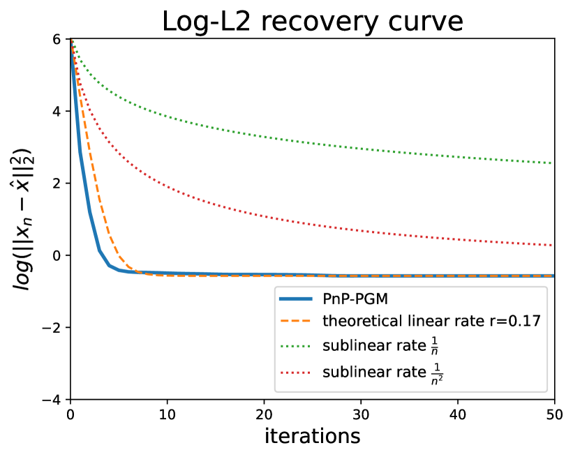
((g)) Log-L2 recovery curve (inpainting)

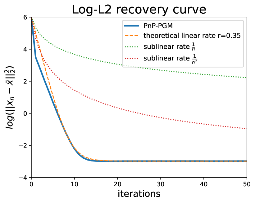
((h)) Log-L2 recovery curve (low blur $\sigma=1.0$)

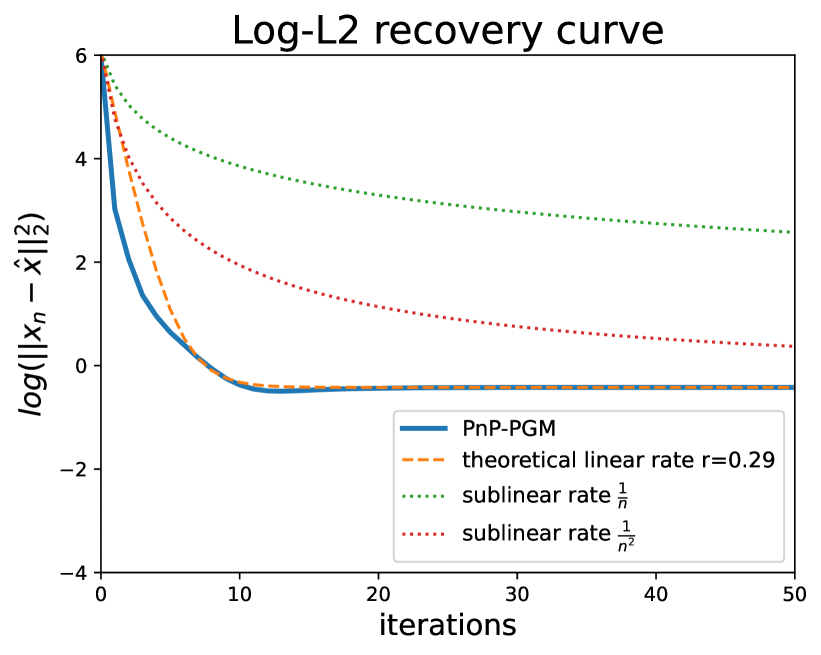
((i)) Log-L2 recovery curve (high blur $\sigma=3.0$)

Figure 2: Experiments for the PnP-PGM algorithm (106) on a synthetic image that is an approximate fixed point of a DRUNet denoiser. For each linear measurement operator, the theoretical linear convergence rate matches well the Log-L2 recovery curve.

4.2.2 Natural Images

In these experiments, we use a DRUNet denoiser trained on natural images (we used the weights provided by the DeepInverse library, see Acknowledgements at the end of the paper) and with the noise level $\eta$ as input (non-blind denoising). To obtain a fixed point of the denoiser, we apply the denoiser on an original natural image multiple times with the entry noise level set to $\eta{=}0.18$ (This parameter is manually set to give good performance). For both images tested (see Figures 3 and 4), we observe that the theoretical linear convergence rate curve (calculated in the same way as the previous experiment) indeed matches well with the convergence curve $\|x_{n}-\hat{x}\|_{2}^{2}$. As expected, the higher blur (i.e. a degraded Restricted Isometry Constant) leads to a decrease in the performance of recovery. Also note that when the linear rate of convergence decreases as in the high blur experiment of Figure 4, it becomes harder to distinguish from a fast sub-linear rate ($\frac{1}{n^{2}}$).

((a)) $y$ inpainting

((b)) $y$ low blur $\sigma=1.0$

((c)) $y$ high blur $\sigma=1.0$

((d)) $x^{*}$ (inpainting)

((e)) $x^{*}$ (low blur $\sigma=1.0$)

((f)) $x^{*}$ (high blur $\sigma=3.0$)

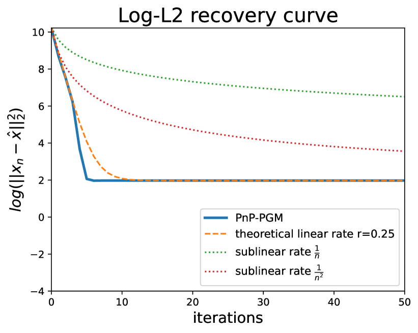
((g)) Log-L2 recovery curve (inpainting)

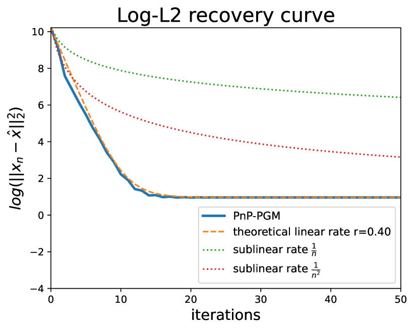
((h)) Log-L2 recovery curve (low blur $\sigma=1.0$)

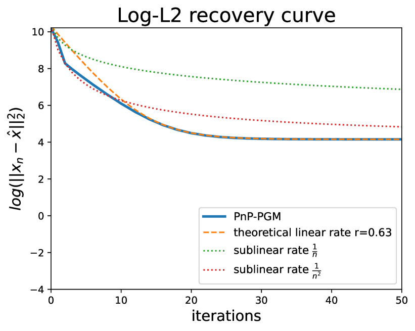
((i)) Log-L2 recovery curve (high blur $\sigma=3.0$)

Figure 3: Experiment of the PnP-PGM algorithm (106) on an image that is an approximate fixed point of the blind denoiser. For each linear operator, the theoretical linear convergence rate matches well the Log-L2 recovery curve.

((a)) $y$ inpainting

((b)) $y$ low blur $\sigma{=}1.0$

((c)) $y$ high blur $\sigma{=}3.0$

((d)) $x^{*}$ (inpainting)

((e)) $x^{*}$ (low blur $\sigma=1.0$)

((f)) $x^{*}$ (high blur $\sigma=3.0$)

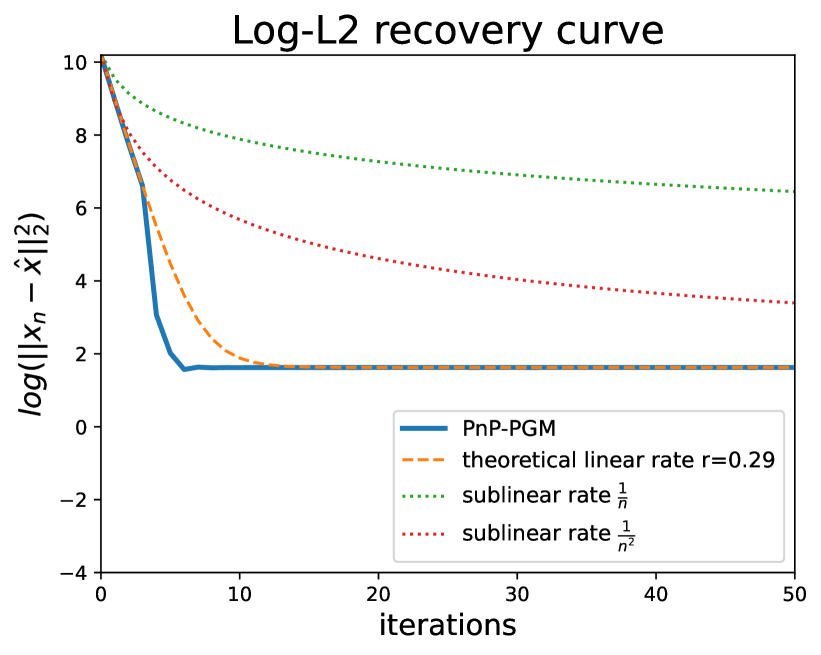
((g)) Log-L2 recovery curve (inpainting)

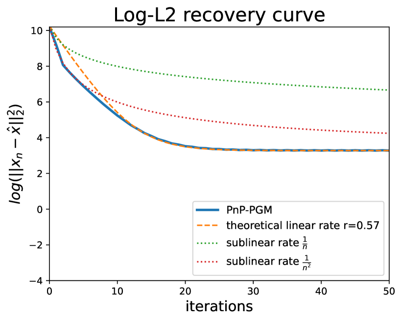
((h)) Log-L2 recovery curve (low blur $\sigma=1.0$)

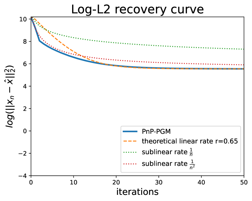
((i)) Log-L2 recovery curve (high blur $\sigma=3.0$)

Figure 4: Experiment of the PnP-PGM algorithm (106) on an image that is an approximate fixed point of the blind denoiser. For each linear operator, the theoretical linear convergence rate matches well the Log-L2 recovery curve.

4.2.3 Comparison between PNP-PGM and GM-RED

We perform the same previous experiments with the GM-RED algorithm, which falls outside the theoretical results provided in this paper. Once again, we observe that the theoretical linear convergence rate matched very well the convergence curve $\|x_{n}-\hat{x}\|_{2}^{2}$ (see Fig. 5, 6, 7). Furthermore, the measured convergence rate of GM-RED is slower than PnP-PGM, reinforcing our initial conjecture. Interestingly, we found that GM-RED was able to obtain a better recovery of our estimated fixed point than PnP-PGM in some experiments (particularly when the measurement operator is better conditioned (low blur)). This could be due to the additional parameter in GM-RED which allows a finer direction towards the low-dimensional model $\Sigma$ induced by the denoiser or simply that our choice of approximate fixed point just matches better the GM-RED algorithm. This opens a question to include approximation error in the projection in our analysis (as was for example done in [15]).

While these experiments do not prove the optimality (with respect to the rate of convergence) of the projected gradient method for low-dimensional recovery, it suggests that our analysis lays out good foundations for a global understanding of low-dimensional recovery with deep priors.

((a)) $y$ inpainting

((b)) $y$ low blur $\sigma=1.0$

((c)) $y$ high blur $\sigma=3.0$

((d)) $x^{\ast}$ (inpainting)

((e)) $x^{\ast}$ (low blur $\sigma{=}1.0$)

((f)) $x^{\ast}$ (high blur $\sigma=3.0$)

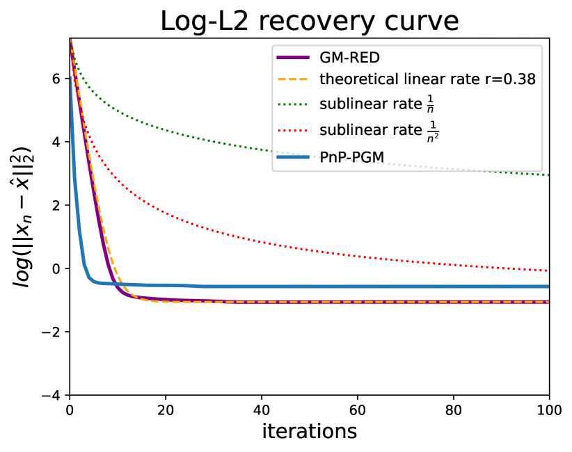
((g)) Log-L2 recovery curve (inpainting)

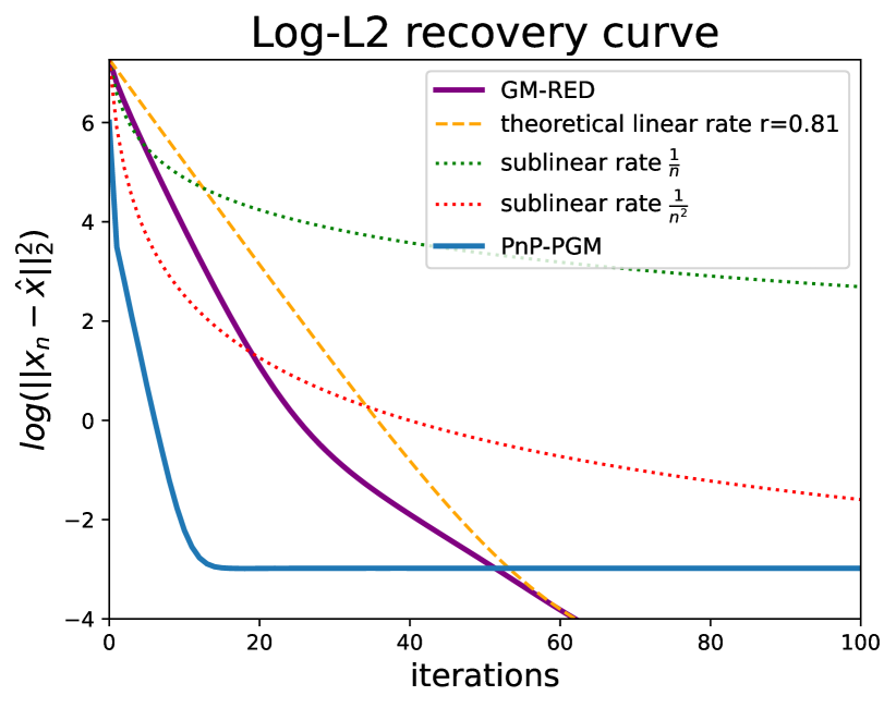
((h)) Log-L2 recovery curve (low blur $\sigma=1.0$)

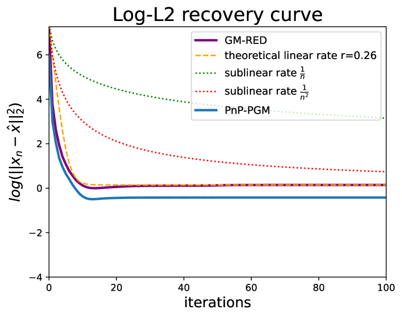
((i)) Log-L2 recovery curve (high blur $\sigma=3.0$)

Figure 5: Experiments of the GM-RED algorithm (106) on a synthetic image for different measurement operators. We observe that GM-RED presents a linear convergence rate. Moreover, the measured convergence rate is slower than PnP-PGM.

((a))

((b))

((c))

((d))

((e))

((f))

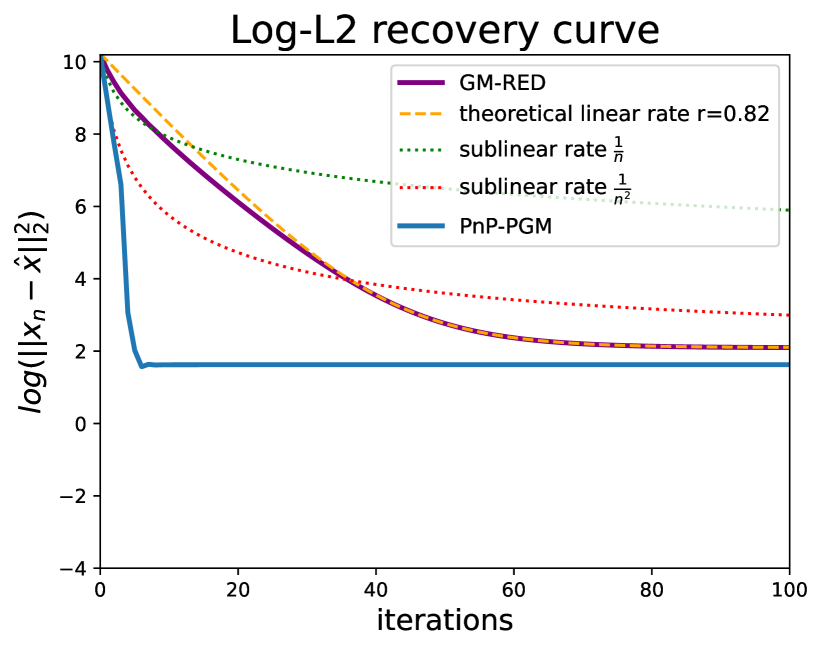
((g))

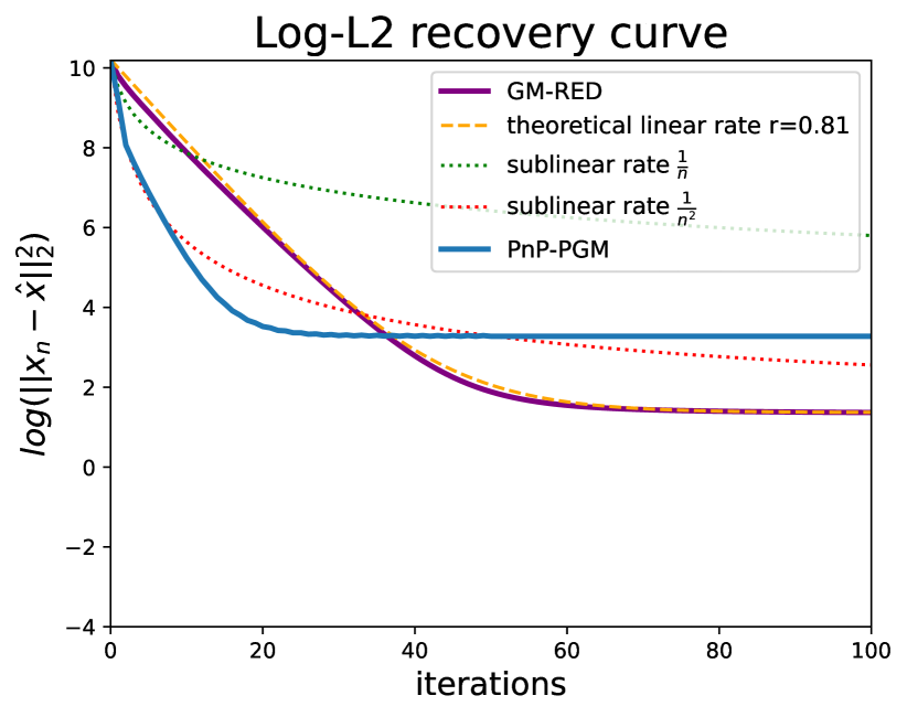
((h))

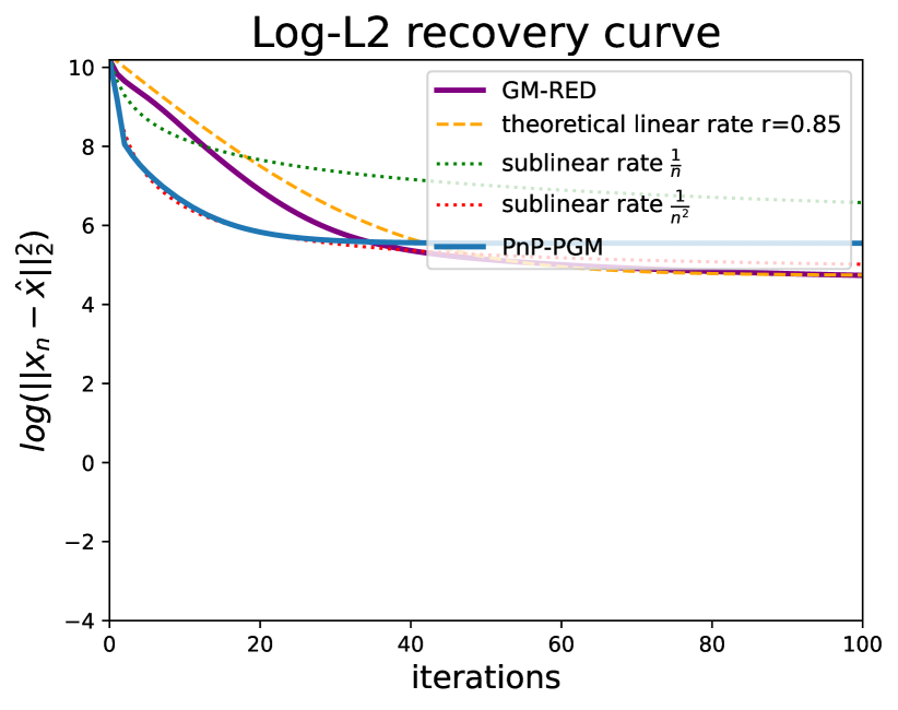
((i))

Figure 6: Experiment of the GM-RED algorithm (106) on the butterfly image for different linear operations. We observe that GM-RED presents a linear convergence rate. Moreover, the measured convergence rate is slower than PnP-PGM.

((a)) $y$ (inpainting)

((b)) $y$ (low blur $\sigma=1.0$)

((c)) $y$ (high blur $\sigma=3.0$)

((d)) $x^{\ast}$ (inpainting)

((e)) $x^{\ast}$ (low blur $\sigma=1.0$)

((f)) $x^{\ast}$ (high blur $\sigma=3.0$)

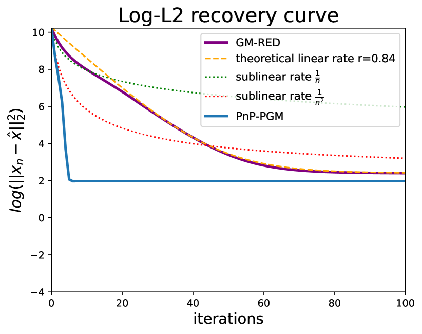
((g))

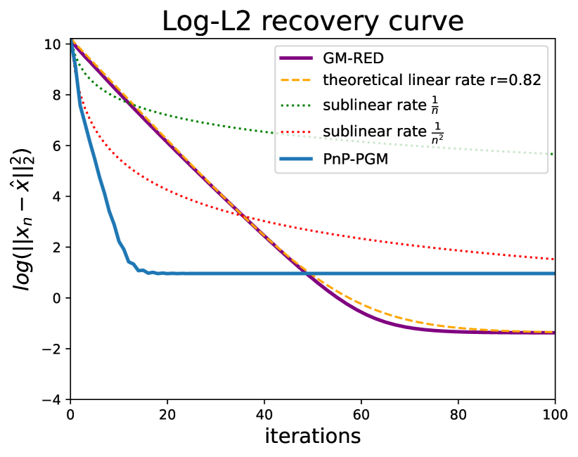
((h))

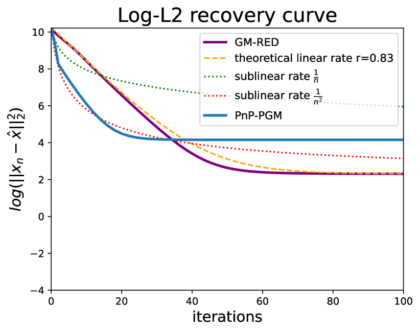
((i))

Figure 7: Experiment of the GM-RED algorithm (106) on the starfish image for different linear operations. We observe that GM-RED presents a linear convergence rate. Moreover, the measured convergence rate is slower than PnP-PGM.

5 Conclusion

We have given a convergence analysis of a class of projected descent algorithms for the recovery of low-dimensional models. This class of algorithm appears naturally when proving the fast convergence of the wider class of algorithms of averaged directions. Our result explicitly quantifies the convergence rate with the restricted isometry constants of the measurement operator and a newly introduced restricted Lipschitz condition on the operator projecting onto the model set. This decouples the role of the geometry of the model and the quality of the measurement operator in the rate of convergence.

More particularly we have shown that the orthogonal projection yields very general guarantees for unions of subspaces. These guarantees can be improved in the case of sparse recovery and iterative hard thresholding, showing that hard thresholding is indeed optimal for the convergence rate (via the restricted Lipschitz constant) when considering the whole class of sparse models (for any sparsity).

Our work lays out the foundation of a theoretical framework for optimal algorithms for the recovery of low-dimensional beyond the variational approach. Many ideas can be explored to generalize this work. Extending to more general classes of algorithms, exploring the tightness of our different results, or studying the impact of the noise in the search for optimality are possible interesting leads. Another possibility would be to add more flexibility to the uniform rate condition and to consider a finite time ”burning” period, i.e. linear convergence guaranteed after a fixed number of iterations.

Our results guarantee linear convergence for solving inverse problems with deep priors. They also raise the question of learning a projection (a denoiser in the plug-and-play framework) with a good restricted Lipschitz constant, thus relaxing the global Lipschitz condition.

6 Acknowledgements

Experiments presented in this paper were carried out using the PlaFRIM experimental testbed, supported by Inria, CNRS (LABRI and IMB), Université de Bordeaux, Bordeaux INP and Conseil Régional d’Aquitaine (see https://www.plafrim.fr). Furthermore, we are grateful to the DeepInverse python library (https://deepinv.github.io/deepinv/index.html) from which the code and weights of the denoiser for natural images was taken from. This work was supported by the French National Research Agency (ANR) under reference ANR-20-CE40-0001 (EFFIREG project), and by PEPR PDE_AI.

References

- [1] H. Attouch, J. Bolte, and B. F. Svaiter, Convergence of descent methods for semi-algebraic and tame problems: proximal algorithms, forward–backward splitting, and regularized gauss–seidel methods, Mathematical Programming, 137 (2013), pp. 91–129.
- [2] S. Bahmani, P. T. Boufounos, and B. Raj, Learning model-based sparsity via projected gradient descent, IEEE Transactions on Information Theory, 62 (2016), pp. 2092–2099.
- [3] R. F. Barber and W. Ha, Gradient descent with non-convex constraints: local concavity determines convergence, Information and Inference: A Journal of the IMA, 7 (2018), pp. 755–806.
- [4] A. Bastounis, A. C. Hansen, and V. Vlačić, The extended smale’s 9th problem–on computational barriers and paradoxes in estimation, regularisation, computer-assisted proofs and learning, arXiv preprint arXiv:2110.15734, (2021).
- [5] A. Beck and N. Hallak, Optimization problems involving group sparsity terms, Mathematical Programming, 178 (2019), pp. 39–67.
- [6] T. Blumensath and M. E. Davies, Normalized iterative hard thresholding: Guaranteed stability and performance, IEEE Journal of selected topics in signal processing, 4 (2010), pp. 298–309.
- [7] A. Bourrier, M. E. Davies, T. Peleg, P. Pérez, and R. Gribonval, Fundamental performance limits for ideal decoders in high-dimensional linear inverse problems, IEEE Transactions on Information Theory, 60 (2014), pp. 7928–7946.
- [8] P. Bürgisser and F. Cucker, Condition: The geometry of numerical algorithms, vol. 349, Springer Science & Business Media, 2013.
- [9] W. Chen, D. Wipf, and M. Rodrigues, Deep learning for linear inverse problems using the plug-and-play priors framework, in ICASSP 2021-2021 IEEE International Conference on Acoustics, Speech and Signal Processing (ICASSP), IEEE, 2021, pp. 8098–8102.
- [10] R. Cohen, M. Elad, and P. Milanfar, Regularization by denoising via fixed-point projection (red-pro), SIAM Journal on Imaging Sciences, 14 (2021), pp. 1374–1406.
- [11] F. Cucker and S. Smale, Complexity estimates depending on condition and round-off error, Journal of the ACM (JACM), 46 (1999), pp. 113–184.
- [12] M. A. Davenport and J. Romberg, An overview of low-rank matrix recovery from incomplete observations, IEEE Journal of Selected Topics in Signal Processing, 10 (2016), pp. 608–622.
- [13] S. Foucart, Hard thresholding pursuit: an algorithm for compressive sensing, SIAM Journal on numerical analysis, 49 (2011), pp. 2543–2563.
- [14] S. Foucart and H. Rauhut, A Mathematical Introduction to Compressive Sensing, Springer, 2013.
- [15] M. Golbabaee and M. E. Davies, Inexact gradient projection and fast data driven compressed sensing, IEEE Transactions on Information Theory, 64 (2018), pp. 6707–6721.
- [16] M. González, A. Almansa, and P. Tan, Solving inverse problems by joint posterior maximization with autoencoding prior, SIAM Journal on Imaging Sciences, 15 (2022), pp. 822–859.
- [17] A. Guennec, J.-F. Aujol, and Y. Traonmilin, Joint structure-texture low dimensional modeling for image decomposition with a plug and play framework, (2024).
- [18] P. Hand and V. Voroninski, Global guarantees for enforcing deep generative priors by empirical risk, IEEE Transactions on Information Theory, 66 (2019), pp. 401–418.
- [19] A. Hauptmann, S. Mukherjee, C.-B. Schönlieb, and F. Sherry, Convergent regularization in inverse problems and linear plug-and-play denoisers, Foundations of Computational Mathematics, (2024), pp. 1–34.
- [20] X. Huo and J. Chen, Complexity of penalized likelihood estimation, Journal of Statistical Computation and Simulation, 80 (2010), pp. 747–759.
- [21] S. Hurault, A. Leclaire, and N. Papadakis, Gradient step denoiser for convergent plug-and-play, in International Conference on Learning Representations (ICLR’22), 2022.
- [22] S. Hurault, A. Leclaire, and N. Papadakis, Gradient step denoiser for convergent plug-and-play, (2022).
- [23] U. S. Kamilov, C. A. Bouman, G. T. Buzzard, and B. Wohlberg, Plug-and-play methods for integrating physical and learned models in computational imaging: Theory, algorithms, and applications, IEEE Signal Processing Magazine, 40 (2023), pp. 85–97.
- [24] U. S. Kamilov and H. Mansour, Learning optimal nonlinearities for iterative thresholding algorithms, IEEE Signal Processing Letters, 23 (2016), pp. 747–751.
- [25] O. Leong, E. O’Reilly, Y. S. Soh, and V. Chandrasekaran, Optimal regularization for a data source, arXiv preprint arXiv:2212.13597, (2022).
- [26] C. Li and B. Adcock, Compressed sensing with local structure: uniform recovery guarantees for the sparsity in levels class, Applied and Computational Harmonic Analysis, 46 (2019), pp. 453–477.
- [27] H. Liu and R. Foygel Barber, Between hard and soft thresholding: optimal iterative thresholding algorithms, Information and Inference: A Journal of the IMA, 9 (2020), pp. 899–933.
- [28] G. Olikier and I. Waldspurger, Projected gradient descent accumulates at bouligand stationary points, arXiv preprint arXiv:2403.02530, (2024).
- [29] G. Ongie, A. Jalal, C. A. Metzler, R. G. Baraniuk, A. G. Dimakis, and R. Willett, Deep learning techniques for inverse problems in imaging, IEEE Journal on Selected Areas in Information Theory, 1 (2020).
- [30] P. Peng, S. Jalali, and X. Yuan, Solving inverse problems via auto-encoders, IEEE Journal on Selected Areas in Information Theory, 1 (2020), pp. 312–323.
- [31] Y. Romano, M. Elad, and P. Milanfar, The little engine that could: Regularization by denoising (red), SIAM Journal on Imaging Sciences, 10 (2017), pp. 1804–1844.
- [32] V. Roulet, N. Boumal, and A. d’Aspremont, Computational complexity versus statistical performance on sparse recovery problems, Information and Inference: A Journal of the IMA, 9 (2020), pp. 1–32.
- [33] J. Scarlett, R. Heckel, M. R. Rodrigues, P. Hand, and Y. C. Eldar, Theoretical perspectives on deep learning methods in inverse problems, IEEE journal on selected areas in information theory, 3 (2022), pp. 433–453.
- [34] J. Tachella, D. Chen, and M. Davies, Sensing theorems for unsupervised learning in linear inverse problems, Journal of Machine Learning Research, 24 (2023), pp. 1–45.
- [35] Y. Traonmilin, J.-F. Aujol, and A. Guennec, Linear rate numerical experiments. https://plmlab.math.cnrs.fr/aguennec/beyond_variation_numerical_final, 2024.
- [36] Y. Traonmilin and R. Gribonval, Stable recovery of low-dimensional cones in hilbert spaces: One rip to rule them all, Applied and Computational Harmonic Analysis, 45 (2018), pp. 170–205.
- [37] Y. Traonmilin, R. Gribonval, and S. Vaiter, A theory of optimal convex regularization for low-dimensional recovery, Information and Inference: A Journal of the IMA, 13 (2024), p. iaae013.
- [38] M. Unser and S. Ducotterd, Parseval convolution operators and neural networks, arXiv preprint arXiv:2408.09981, (2024).
- [39] S. V. Venkatakrishnan, C. A. Bouman, and B. Wohlberg, Plug-and-play priors for model based reconstruction, in 2013 IEEE global conference on signal and information processing, IEEE, 2013, pp. 945–948.
- [40] T. Vu and R. Raich, On asymptotic linear convergence of projected gradient descent for constrained least squares, IEEE Transactions on Signal Processing, 70 (2022), pp. 4061–4076.
- [41] K. Zhang, Y. Li, W. Zuo, L. Zhang, L. Van Gool, and R. Timofte, Plug-and-play image restoration with deep denoiser prior, IEEE Transactions on Pattern Analysis and Machine Intelligence, 44 (2021), pp. 6360–6376.