When Does Interference Matter?
Decision-Making in Platform Experiments

Abstract

This paper investigates decision-making in A/B experiments for online platforms and marketplaces. In such settings, due to constraints on inventory, A/B experiments typically lead to biased estimators because of interference between treatment and control groups; this phenomenon has been well studied in recent literature. By contrast, there has been relatively little discussion of the impact of interference on decision-making. In this paper, we analyze a benchmark Markovian model of an inventory-constrained platform, where arriving customers book listings that are limited in supply; our analysis builds on a self-contained analysis of general A/B experiments for Markov chains. We focus on the commonly used frequentist hypothesis testing approach for making launch decisions based on data from customer-randomized experiments, and we study the impact of interference on (1) false positive probability and (2) statistical power.

We obtain three main findings. First, we show that for monotone treatments—i.e., those where the treatment changes booking probabilities in the same direction relative to control in all states—the false positive probability of the naïve difference-in-means estimator with classical variance estimation is correctly controlled. This result stems from a novel analysis of A/A experiments with arbitrary dependence structures, which may be of independent interest. Second, we demonstrate that for monotone treatments, the statistical power of this naïve approach is higher than that of any similar pipeline using a debiased estimator. Taken together, these two findings suggest that platforms may be better off not debiasing when treatments are monotone. Third, using simulations, we investigate false positive probability and statistical power when treatments are non-monotone, and we show that the performance of the naïve approach can be arbitrarily worse in such cases.

Our results have important implications for the practical deployment of debiasing strategies for A/B experiments. In particular, they highlight the need for platforms to carefully define their objectives and understand the nature of their interventions when determining appropriate estimation and decision-making approaches. Notably, when interventions are monotone, the platform may actually be worse off by pursuing a debiased decision-making approach.

1 Introduction

Online platforms and marketplaces routinely use randomized controlled trials, also known as A/B experiments to test changes to their market design, such as the introduction of new algorithms, new features, or pricing and fee changes. For example, an online marketplace for lodging might use A/B experiments to test the impact of a change in the description of listings on overall bookings; or a ride-sharing marketplace might use A/B experiments to test the impact of lowering the surge price on overall rides. In a typical approach for such experiments, customers (i.e., users looking to purchase) are randomized to treatment (i.e., the new product feature) or control (i.e., the existing product feature), using a simple i.i.d. Bernoulli randomization scheme. Of interest to the platform is the global treatment effect ($\mathsf{GTE}$): the difference in aggregate sales if the entire market is in treatment as compared to control. Once outcomes (e.g., bookings or rides) are collected after the experiment, a simple difference-in-means (DM) estimator (denoted $\widehat{\mathsf{GTE}}$) is used to estimate the $\mathsf{GTE}$.

A key challenge for these platforms is that this simple estimation approach suffers from interference between treatment and control units, because of the constrained inventory on each side of the platform. For example, consider an A/B experiment in an online marketplace for lodging that randomizes arriving customers to treatment or control (i.e. customer-side randomization, or CR). Because these customers interact with the same inventory of listings, customers’ booking outcomes impact the state of the market as seen by subsequent arriving customers. This interference effect leads $\widehat{\mathsf{GTE}}$ to be biased relative to the $\mathsf{GTE}$. Extensive recent literature has investigated conditions characterizing the magnitude of this bias, conditions under which it is magnified, and methods for debiasing (i.e., combinations of designs and/or estimators that estimate $\mathsf{GTE}$ with low bias). See Section 2 for related references.

Despite this extensive attention on bias and debiasing of estimates of the treatment effect, thus far there has been limited investigation of the impact of bias on decision-making. In the typical use case of A/B experiments, beyond estimation of the treatment effect, platforms are also making a decision about whether or not to launch the treatment change being tested to the entire marketplace. What is the impact of interference on these decisions? Our paper focuses on this question.

Our main contribution is an analysis and characterization of the impact of interference in a benchmark model of decision-making. As we show, for a wide range of interventions, despite the presence of interference a platform may actually be no worse off (and possibly better off, in a sense we make precise) if they make decisions using the “naïve” DM estimation approach, along with the associated classical variance estimator. We further discuss conditions under which debiasing can be essential to make correct decisions.

We consider a frequentist decision-making process that is quite commonly used after A/B experiments in online platforms, based on hypothesis testing. After calculating $\widehat{\mathsf{GTE}}$, the platform computes an associated naïve variance estimator assuming observations were i.i.d. (i.e., that there is no interference or correlation between observations); we denote this variance estimator $\widehat{\mathrm{Var}}$. (Note that because interference is present, in general $\widehat{\mathrm{Var}}$ will also be biased for the true variance of $\widehat{\mathsf{GTE}}$.) Using these quantities, the platform forms the standard t-test statistic, $T=\widehat{\mathsf{GTE}}/\sqrt{\widehat{\mathrm{Var}}}$. The platform then supposes that under the null hypothesis $H_{0}$ that $\mathsf{GTE}=0$, $\hat{T}$ is approximately distributed according to a standard normal random variable; this assumption is valid if data is independent across observations, but not necessarily in the presence of interference. In particular, $\hat{T}$ is then compared to the tail quantiles of a standard normal random variable, and $H_{0}$ is rejected if $|\hat{T}|$ is sufficiently large. (Commonly, $H_{0}$ is rejected if $|\hat{T}|>1.96$.) (Note that in practice, the platform will typically only launch the intervention if $H_{0}$ is rejected, and the estimate $\widehat{\mathsf{GTE}}$ is in a beneficial direction for the platform, e.g., positive for metrics like revenue, negative for metrics like cost.)

Although the frequentist hypothesis testing paradigm faces many criticisms in practice, it is also widely deployed and prevalent in the decision-making practices of technology companies generally, and online platforms and marketplaces in particular. Typically this decision-making pipeline is evaluated based on two criteria. First is the false positive probability (or type I error rate): what is the chance of mistakenly rejecting $H_{0}$, when $H_{0}$ is true, i.e., $\mathsf{GTE}=0$, and in particular, does the false positive probability match the desired control in the decision rule? (For example, when a cutoff of $|\hat{T}|>1.96$ is used, the false positive probability should be no more than $5\%$.) Second is the statistical power, or the complement of the false negative probability (type II error rate): what is the chance of correctly rejecting $H_{0}$, under a specific alternative for which $\mathsf{GTE}\neq 0$? We analyze and characterize these two quantities in the presence of interference.

Formally, to carry out our analysis, we consider a general Markovian model of a platform with finitely many listings; similar models have been considered by prior papers as well to model interference (see Section 2). Customers arrive over time according to a Poisson process, and can book a listing if one is available; our model allows customers to have heterogeneous preferences, but listings are homogeneous. Once booked, a listing remains occupied for some time before becoming available to book again. Our model assumes that an arriving customer’s booking probability is lower when fewer listings are available, as is the case in real-world platforms. We consider a natural class of treatments: those that change the state-dependent booking probabilities of customers. We suppose that the platform runs a Bernoulli randomized CR experiment, collects data on the booking outcomes of $N$ arriving customers, and executes the decision-making pipeline above.

A challenge arises here because in general, the null hypothesis $H_{0}$ that $\mathsf{GTE}=0$ does not completely determine the distribution of observations: informally, this is because there are many configurations of treatment and control booking probabilities that lead to the the same value of $\mathsf{GTE}$. (In statistical terms, $H_{0}:\mathsf{GTE}=0$ is a composite null hypothesis, rather than a simple null hypothesis.) To make progress, we focus our attention on monotone treatments: these are treatments where the booking probabilities of customers move in the same direction (i.e., higher or lower) relative to control, in all states. For example, if a platform raises fees, then it is reasonable to assume that regardless of the state, this will lower booking probabilities. Prior literature has also studied the bias in platform experiments when treatments are monotone; see, e.g., [16, 25, 32, 8, 9].

Crucially, we show that if the treatment is known to be monotone and $H_{0}$ holds, then all booking probabilities in treatment and control are identical. In other words, the assumption of monotone treatments, together with $\mathsf{GTE}=0$, determines that the experimental observations correspond to an A/A experiment, i.e., tests where the same version of a product or feature is tested against itself (so that the joint distribution of observations in both the global treatment and global control conditions is the same). Companies routinely use A/A experiments to validate the experimental setup, and ensure the accuracy of their testing infrastructure (see, e.g., [36, 42, 48]). For example, an e-commerce platform might run an A/A test to ensure that user traffic is being evenly split across different servers, or a streaming service could use an A/A test to confirm that their recommendation algorithm is not unintentionally favoring one group of users over another. Such experiments are a core aspect of the validation of experimentation within any organization that adopts A/B testing.

Our first main contribution is to show that when treatments are monotone, the false positive probability of the decision-making pipeline above is correctly controlled (Section 4). We obtain this insight by considering a far more general setting of A/A experiments, allowing for arbitrary (even non-Markovian) dependence structure between observations, which may be of independent interest to practitioners. Ou central surprising finding that in A/A experiments, the estimator $\widehat{\mathrm{Var}}$ is unbiased for the true variance of $\mathsf{GTE}$, despite no estimation of covariance between observations. We use a novel stochastic exchangeability argument to establish this result (see Theorem A.2). An associated central limit theorem is also given in a general setting of Markovian system dynamics (see Theorem A.3). Application of these results to our inventory-constrained platform yields the desired control of false positive probability under monotone treatments (Theorems 3.2 and 4.1).

Our second main contribution is to show that when treatments are monotone, the statistical power of the decision-making pipeline above is likely to be higher than that achieved by any similar pipeline using a debiased estimator (Section 5). We show this by imagining that the platform has access to an alternative estimator $\hat{\theta}$ which is unbiased for the $\mathsf{GTE}$, and alongside $\hat{\theta}$ is able to exactly compute the variance $\mathrm{Var}(\hat{\theta})$. We suppose the platform could form a test statistic $\hat{U}=\hat{\theta}/\sqrt{\mathrm{Var}(\hat{\theta})}$. Through a combination of theory and simulation, our finding is that the magnitude of $\hat{T}$ is generally larger than that of $\hat{U}$. Theoretically, using stochastic monotonicity arguments applied to the underlying experiment Markov chain, we show that both in finite samples and asymptotically, $\widehat{\mathsf{GTE}}$ is larger than $\mathsf{GTE}$ (Theorems 5.1 and 5.2); in finite samples in particular, this is a result that has not been shown previously. On the other hand, leveraging a Cramér-Rao lower bound on variance of any unbiased estimator given in [11], we show via simulation that $\widehat{\mathrm{Var}}$ is generally smaller than $\mathrm{Var}({\hat{\theta}})$ (a common bias-variance tradeoff in constructing unbiased estimators). Together, these results imply that using $\hat{T}$ yields higher power than using the unbiased estimation strategy $\hat{U}$.

These two contributions together suggest the surprising finding that when treatments are monotone, and the platform uses the decision-making pipeline above, then the platform is likely strictly better off not debiasing. Our third main contribution is to investigate the robustness of this finding, by studying via simulation the consequences when treatments are non-monotone (Section 6). We consider a natural class of treatments: those that might increase booking probabilities when many listings are available, but lower booking probabilities when few listings are available. For example, a ride-sharing platform may want to test changing prices in a state-dependent manner, lowering prices relative to control when many drivers are available, but raising prices relative to control when few drivers are available. We show via simulation example that with non-monotone treatments, the performance of the naïve decision-making pipeline above using $\hat{T}$ can be arbitrarily worse than a debiased strategy using $\hat{U}$, both in terms of false positive probability and in terms of statistical power.

Taken together, our findings have important implications for the deployment of debiasing strategies in practice. Many of the debiasing methods suggested in the literature are nontrivial, and from a practical standpoint, there can be significant organizational friction in adopting these alternatives. Our work suggests that understanding the nature of the intervention is important to determining whether the additional effort in debiasing is worthwhile; and indeed, for monotone interventions and CR experiments, it may be strictly preferable not to debias. Of course, platforms have many other goals as well in A/B experimentation; for example, often the precise estimate of the treatment effect is of interest (e.g., when evaluating the benefits of an intervention against the cost of deployment), in which case debiasing is essential to obtain an accurate estimate of the true $\mathsf{GTE}$. Broadly, our work argues that platforms should carefully define their objectives and inferential goals in determining an appropriate approach to estimation and decision-making.

The remainder of the paper is organized as follows. In Section 2, we present related work. In Section 3, we introduce our benchmark inventory-constrained platform model, as well as the decision-making pipeline outlined above, and introduce the concept of monotone interventions. In Section 4, we present our general results for A/A experiments (Section 4.1), and use it to characterize false positive probability under monotone treatments, both in finite samples and asymptotically (Section 4.2). In Section 5, we study statistical power, again in finite samples (Section 5.1) and asymptotically (Section 5.2). Finally, in Section 6, we present simulation results investigating false positive probability and statistical power when treatments are non-monotone. We conclude in Section 7.

We collect together supplementary material in several appendices. Appendix A may be of independent interest to other researchers working on experimentation in Markovian settings, where we present together (in a self-contained manner) central limit theorems and associated analysis for both A/B and A/A experiments when the underlying treatment and control systems are general Markov chains. (We use these results in our analysis of our inventory-constrained platform model.) Appendix B contains proofs of several results in the main paper. Appendix C contains additional simulation results.

2 Related work

In this section we discuss three related streams of work: (1) Interference in experiments, particularly in networks and markets; (2) the use of Markov chain models to study experimental design and estimation; and (3) the practice of A/B experimentation, and particularly making decisions from A/B experiments.

Interference in experiments.

A rich literature in causal inference broadly, and more recently in the study of networks and markets, has considered interference between treatment and control groups in experiments. We refer the reader to [21, 43, 22, 18] for broader discussion of interference. In the literature on social networks, a range of papers have studied the role of interference on bias of estimation, as well as approaches to obtain unbiased estimates of direct and indirect treatment effects; see, e.g., [1, 37, 47, 10] for early influential work in this area. We note that [2] provides exact p-values in a randomization inference framework for network experiments, which correctly control false positive probability.

More recently, extensive attention has also been devoted to interference in marketplace and platform experiments; see, e.g., [6, 50, 25, 32, 4, 39, 8] as examples of this line of work. As discussed in Section 1, this prior work primarily focuses on the presence of bias in the use of “naive” estimators of $\mathsf{GTE}$, such as the difference-in-means estimator, and often investigates designs and/or estimators to reduce that estimation bias. Many of the papers that study Markov chain models in the context of experimentation are also specifically motivated by similar questions in marketplace experimentation, as we discuss below. In contrast to these works, our emphasis is on understanding false positive probability and statistical power when the difference-in-means estimator (and its associated naive variance estimator) are used for decision-making, in spite of interference and the resulting bias.

We note that a number of papers have specifically considered interference in the context of price experimentation, including [6, 50, 33, 9, 41]. One interesting issue that can arise there is that optimization based on the estimated effect of a price change on revenue or profit can lead the decision-maker astray, as (due to interference) the estimator can have the wrong sign compared to the true $\mathsf{GTE}$ (see [9, 41]). We consider bookings as our primary outcome metric in our paper, so our findings should be viewed as distinct from and complementary to this line of work.

Markov chain models of experiments.

A number of recent papers have employed Markov chain models as a structural representation of treatment and control in experimental settings; see, e.g., [14, 19, 25, 11, 12, 33, 7], as well as related work on off-policy evaluation for Markov decision processes [34, 27, 20, 38].

Of these papers, the most related to our own work are [25, 11, 33], all of which consider a queueing model to capture interference due to limited inventory, as arises in marketplaces. In [25], the paper focuses on analysis of estimation bias in a mean-field regime, as well as an alternative two-sided randomized design and associated estimator to mitigate bias; a similar design was contemporaneously proposed and studied in [4]. In [33], the paper exploits knowledge of the queueing model to construct low-variance estimators in the presence of congestion, in the context of pricing experiments that impact arrival rates. In [11], the paper studies an estimator based on an (estimated) difference in $Q$-values, to reduce bias in Markov chain experiments in general, and marketplace experiments in particular. We leverage a Cramér-Rao lower bound from [11] in our analysis of asymptotic statistical power in Section 5.2.

These papers on Markov chain models for experiments do not consider the impact of interference on the resulting decisions that are made based on the experiment. One recent exception is [7]; they study a setting with interference arising due to capacity constrained interventions, and (using a queueing-theoretic approach) show that the statistical power to detect a positive effect is not monotonic in the number of subjects recruited, as is the case in standard experiments without interference.

The practice of A/B experimentation.

Finally, our paper is connected to a wide literature on the use of A/B experiments in industry to make decisions about features, algorithms, and products. For a broad overview of the relevant considerations in this space, we refer the reader to [30]. In general, this literature considers experiments where data are independent observations, and so does not consider the role of interference.

A number of different lines of work consider potential challenges in the decision-making pipeline that follows A/B experiments. For example, a range of papers (see, for example, [23, 24, 17]) study methods to ameliorate the inflation of false positive probability that arises when decision-makers continuously monitor experiments. A recent paper notes that because most experiments do not succeed in practice, false positives may be more common than practitioners realize [29].

Several papers highlight the fact that if companies evaluate experiments based on the returns generated by the “winning” variations, and if there are opportunity costs to experimentation, then running many, shorter experiments is ideal to find the potentially big winners (see, e.g., [13, 46, 3]). More generally, we note that if one is interested in simply picking the best alternative among many possible features, products, or algorithm designs, then the extensive literature on multi-armed bandit algorithms (see, e.g., [31] for a recent textbook treatment) provides appropriate methodology. In our paper, by contrast, the emphasis is specifically on the impact of interference for decisions made from A/B experiments that follow the paradigm of randomized controlled trials.

3 Experiments and decision-making in inventory-constrained platforms

In this section, we introduce a benchmark model for interference, experimentation, estimation, and decision-making in an inventory-constrained platform. Using this model, we articulate the key questions studied in this paper: If a platform follows common practice in running experiments by using a hypothesis test for the null hypothesis that the treatment effect is zero, what is the probability of false positives (type I error rate) and false negatives (type II error rate, or the complement of statistical power)?

In Section 3.1, we present the details of the stochastic model we study. In Section 3.2, we describe experiments and, estimation. In Section 3.3, we provide asymptotic descriptions of the estimators: a central limit theorem for the difference-in-means estimator, and an associated limit for the variance estimator). In Section 3.4 we formalize the null hypothesis that the global treatment effect is zero, and describe the standard t-test statistic for this hypothesis. Finally, in Section 3.5, we specialize our setting to monotone interventions, and define the false positive probability and statistical power.

3.1 A model of an inventory-constrained platform

We consider a platform where customers (the demand side) arrive over time, and can choose to book from a finite supply of listings; for example, such a model is a reasonable abstraction of a two-sided marketplace. At a high level, we model such a platform as a Markovian birth-death queueing system. In our model customers arrive over time, and can choose to book a listing if one is available when they arrive. If they book, then the listing is made unavailable for a period of time, before being made available again for booking. Similar models have previously been considered in the context of experiments (see, e.g., [25, 11, 33]).

The formal details of our model are as follows. Throughout we use boldface to denote vectors and matrices.

Time.

The system evolves over an infinite continuous time horizon $t\in[0,\infty)$.

Listings.

The system consists of $K$ homogeneous listings.

State description.

At each time $t$, each listing can be either available or booked (i.e., occupied by a customer who previously booked it). We let $X_{t}\in\{0,\dots,K\}$ denote the number of booked listings at time $t$.

Customers.

Customers arrive sequentially to the platform and can book a listing if one is available, i.e., if $X_{t}<K$ for a customer who arrives at time $t$. We give arriving customers sequential indices $1,2,\ldots$. Each customer $i$ has a type $\gamma_{i}\in\Gamma$, where $\Gamma$ is a finite nonempty set that represents customer heterogeneity. Customers of type $\gamma$ arrive according to a Poisson process with rate $\lambda_{\gamma}>0$.

We assume that when a customer of type $\gamma$ arrives to the platform with $k$ booked listings, the customer will book with probability $p_{\gamma}(k)$. We let $Y_{i}\in\{0,1\}$ denote the booking outcome of customer $i$ (where $1$ denotes that they book a listing, and $0$ denotes that they do not make a booking).

Throughout the paper, we make the natural assumption that the booking probabilities are strictly decreasing in the number of booked listings, as formalized below. For completeness we also define $p_{\gamma}(K)=0$ for all $\gamma$: no listings can be booked if none are available. (We assume the inequalities are strict in the following definition largely for technical simplicity of the remainder of our presentation.)

Assumption 3.1.

For any $\gamma\in\Gamma$, there holds $p_{\gamma}(0)>p_{\gamma}(1)>\cdots>p_{\gamma}(K-1)>p_{\gamma}(K)=0$.

In our subsequent development it will be convenient to abstract away from customer heterogeneity, by defining $\lambda=\sum_{\gamma}\lambda_{\gamma}$, and:

$$p(k)=\frac{1}{\lambda}\sum_{\gamma}\lambda_{\gamma}p_{\gamma}(k).$$

Note that $p(k)$ is the probability a listing is booked conditional on an arrival, if $k$ listings are available. Further, note that as long as each $\boldsymbol{\mathrm{p}}_{\gamma}$ satisfies Assumption 3.1, then $\boldsymbol{\mathrm{p}}$ satisfies this assumption as well.

Listing holding times.

We assume that when $X_{t}=k$, i.e., $k$ listings are booked, the time until at least one of those listings becomes available is exponential with parameter $\tau(k)$.

We make the following natural monotonicity assumption on the holding time parameters $\tau(k)$. Qualitatively, this assumption guarantees that as the available inventory of listings becomes more scarce, the rate at which listings become available again can only increase. Note that this allows for a wide range of specifications. For example, if $\tau(k)=k\tau$ for a fixed constant $\tau$, then booked listings have independent exponential holding times with mean $1/\tau$. On the other hand, if $\tau(k)=\tau$ for all $k$, then the service system operates as a single server queueing system with finite buffer capacity $K$.

Assumption 3.2.

For $k=1,\ldots,K-1$, there holds $0<\tau(k)\leq\tau(k+1)$.

Steady state.

With the preceding assumptions, the state $X_{t}$ is a continuous time Markov chain, with generator $\boldsymbol{\mathrm{Q}}$ defined as follows:

$$\boldsymbol{\mathrm{Q}}=\begin{bmatrix}-\lambda p(0)&\lambda p(0)&0&\dots&0\\ \tau(1)&-\tau(1)-\lambda p(1)&\lambda p(1)&\dots&0\\ \vdots&\vdots&\vdots&\vdots&\vdots\\ 0&\dots&0&\tau(K)&-\tau(K)\end{bmatrix}.$$ (1)

Under our assumptions, we note that the Markov chain above is a birth-death chain that is irreducible on a finite state space, with a unique steady state distribution $\boldsymbol{\mathrm{\pi}}=(\pi(0),\ldots,\pi(K))$ defined by $\boldsymbol{\mathrm{\pi}}\boldsymbol{\mathrm{Q}}=0$. Note that $\boldsymbol{\mathrm{\pi}}$ depends on the parameters of the system through the generator $\boldsymbol{\mathrm{Q}}$, in particular, the aggregate arrival rate $\lambda$, the average booking probabilities $p(k)$ for each $k$, and the holding time parameters $\tau(k)$ for each $k$.

Steady state average booking probability.

A key statistic of interest to us is the steady state average booking probability of the service system, denoted $\rho$. This is the probability an arriving customer books a listing in steady state, and can be obtained as:

$$\rho=\sum_{k}\pi(k)p(k).$$ (2)

3.2 Experiments and estimation

In this section, we model treatments that change the system dynamics by altering customer customer booking behavior. We also define a canonical experiment design and difference-in-means estimator for the resulting treatment effect, as well as an associated variance estimator. The formal details of our approach are as follows; similar models have been considered by prior work as well (see, e.g., [25, 11, 33]).

Binary treatment.

We consider interventions that change the booking probability of a customer of type $\gamma$ in state $k$. Formally, we denote treatment by $1$ and control by $0$, and consider an expanded type space for customers: for each type $\gamma\in\Gamma$, we let $(\gamma,1)$ denote a treatment customer of type $\gamma$, and $(\gamma,0)$ denote a control customer of type $\gamma$. For treatment status $z\in(0,1)$, we let $p_{\gamma,z}(k)$ denote the probability a type $(\gamma,z)$ customer books in state $k$. We again emphasize that we assume these booking probabilities satisfy Assumption 3.1.

As before, we average over types $\gamma$ and obtain:

$$p_{z}(k)=\frac{1}{\lambda}\sum_{\gamma}\lambda_{\gamma}p_{\gamma,z}(k).$$

We refer to $p_{1}(k)$ (resp., $p_{0}(k)$) as the treatment (resp., control) booking probability in state $k$.

Bernoulli customer randomization (CR).

We assume the platform runs an experiment on the first $N$ customers to arrive. We assume a parameter $a\in[0,1]$ such that each arriving customer is randomized independently to treatment with probability $a$, i.e., for each customer $i$, their treatment status $Z_{i}$ is an independent Bernoulli$(a)$ random variable. For notational convenience, we define $N_{1}=\sum_{i}Z_{i}$, $N_{0}=\sum_{i}(1-Z_{i})$.

System dynamics in a CR experiment.

In a CR experiment, the system dynamics again evolve as a Markovian birth-death queueing system as before, but with arrival rates that are mediated by assignment to treatment or control. Formally, define:

$$q_{a}(k) =(1-a)p_{0}(k)+ap_{1}(k);$$ (3)

this is the probability that an arriving customer books in a CR experiment with treatment allocation $a$, when the state is $k$. Then the generator for the system dynamics in a CR experiment is again given by (1), but with $\lambda p(k)$ replaced by $\lambda q_{a}(k)$.

We let $\boldsymbol{\mathrm{\pi}}_{a}=(\pi_{a}(0),\ldots,\pi_{a}(K))$ denote the steady state distribution of this Markov chain. (Note, though, that the experiment will only last for a random finite time, since it involves a sample size of $N$ customers.)

Estimand: The global treatment effect.

With these definitions, the global treatment condition is the special case where $a=1$, and the global control condition is the special case where $a=0$. We can then define steady state average booking probabilities: for $z=0,1$, we have $\rho_{z}=\sum_{k}\pi_{z}(k)p_{z}(k)$.

We define the estimand as the steady state global treatment effect (or global average treatment effect):

$$\mathsf{GTE}=\rho_{1}-\rho_{0}.$$ (4)

Difference-in-means (DM) estimator.

A common practice is to employ a difference-in-means (DM) estimator to formulate a test statistic. We denote this estimator by $\widehat{\mathsf{GTE}}_{N}$. Formally:

$$\widehat{\mathsf{GTE}}_{N}=\overline{Y}(1)-\overline{Y}(0),$$ (5)

where:

$$\overline{Y}(1)=\frac{\sum_{i}Z_{i}Y_{i}}{N_{1}};\quad\overline{Y}(0)=\frac{\sum_{i}(1-Z_{i})Y_{i}}{N_{0}}.$$

(Recall $N_{1}$ and $N_{0}$ are the number of treated and control units, respectively.) All summations are over all $N$ units.

Note that $\widehat{\mathsf{GTE}}_{N}$ is not well defined if either $N_{1}=0$ or $N_{0}=0$; we will use conditioning to avoid this event in our analysis.

The naive variance estimator and bias.

Associated to the DM estimator is a “naive” variance estimator, defined as follows:

$$\widehat{\mathrm{Var}}_{N}=\frac{1}{N_{1}(N_{1}-1)}\sum_{i}Z_{i}(Y_{i}-\overline{Y}(1))^{2}+\frac{1}{N_{0}(N_{0}-1)}\sum_{i}(1-Z_{i})(Y_{i}-\overline{Y}(0))^{2}.$$ (6)

Note that this estimator assumes that observations are independent draws across treatment and control groups, and i.i.d. draws within treatment and control groups; if these assumptions held, the variance estimator would be unbiased for the true variance of the DM estimator.

Again, note that $\widehat{\mathrm{Var}}_{N}$ is not well defined if either $N_{1}\leq 1$ or $N_{0}\leq 1$; again, we will use conditioning to avoid this event in our analysis.

Interference and bias.

We note that the Bernoulli CR experiment together with the DM estimator and the naive variance estimator suffers from interference, i.e., violation of the stable unit treatment value assumption (SUTVA) [22]. This assumption requires that the outcome of one unit (in this case, the booking outcome of a customer) does not depend on the treatment assignment of other units (i.e., other customers). However, because inventory is constrained in this service system, there is interference over time between customers: if a customer books a listing, then that listing may be unavailable for a subsequent customer.

In general, this interference effect will imply that both the estimator $\widehat{\mathsf{GTE}}_{N}$ will be biased (as has been extensively discussed in the literature, cf. Section 2), and the variance estimator $\widehat{\mathrm{Var}}_{N}$ will be biased as well.

3.3 A central limit theorem

In this section we state a central limit theorem (CLT) for $\widehat{\mathsf{GTE}}_{N}$ and also provide an asymptotic characterization of $\widehat{\mathrm{Var}}_{N}$. We prove this result in a more general setting, considering A/B experiments between two arbitrary Markov chains on a finite state space; see Appendix A.4 for details.

We require the following definitions. Fix a treatment allocation parameter $a$, and let $\boldsymbol{\mathrm{\pi}}_{a}$ be the steady state distribution as above. We define the average direct effect ($\mathsf{ADE}_{a}$) as follows [18]:

$$\mathsf{ADE}_{a}=\sum_{k}\pi_{a}(k)p_{1}(k)-\sum_{k}\pi_{a}(k)p_{0}(k).$$ (7)

This is the difference in treatment and control booking probabilities, but when the distribution over states is given by the steady state distribution from the experiment. Since, in general, the steady state distribution $\boldsymbol{\mathrm{\pi}}_{a}$ neither matches global treatment $\boldsymbol{\mathrm{\pi}}_{1}$ nor global control $\boldsymbol{\mathrm{\pi}}_{0}$, in general $\mathsf{ADE}_{a}\neq\mathsf{GTE}$.

Next, define the following quantities for $z,z^{\prime}\in\{0,1\}$:

$$V(z) =\mathbb{E}_{\boldsymbol{\mathrm{\pi}}_{a}}\left[\left(Y_{1}-\sum_{k}\pi_{a}(k)p_{z}(k)\right)^{2}\Bigg{|}Z_{1}=z\right]$$

$$=\sum_{k}\pi_{a}(k)\left(p_{z}(k)\left(1-\sum_{k}\pi_{a}(k)p_{z}(k)\right)^{2}+(1-p_{z}(k))\left(\sum_{k}\pi_{a}(k)p_{z}(k)\right)^{2}\right);$$

$$=\mathrm{Var}_{\boldsymbol{\mathrm{\pi}}_{a}}(Y_{1}|Z_{1}=z);$$ (8)

$$C_{j}(z,z^{\prime}) =\mathbb{E}_{\boldsymbol{\mathrm{\pi}}_{a}}\left[\left(Y_{1}-\sum_{k}\pi_{a}(k)p_{z}(k)\right)\left(Y_{j}-\sum_{k}\pi_{a}(k)p_{z^{\prime}}(k)\right)\Bigg{|}Z_{1}=z,Z_{j}=z^{\prime}\right].$$

$$=\mathrm{Cov}_{\boldsymbol{\mathrm{\pi}}_{a}}(Y_{1},Y_{j}|Z_{1}=z,Z_{j}=z^{\prime}).$$ (9)

In these expressions, the subscript $\boldsymbol{\mathrm{\pi}}_{a}$ on the expectations indicates that the chain is initialized in the steady state distribution $\boldsymbol{\mathrm{\pi}}_{a}$ just prior to the arrival of the first customer. These quantities are the conditional variance and covariance of rewards, respectively, given the treatment assignments.

The following central limit theorem comes from an application of Theorem A.1 in Appendix A to this setting; see the discussion in Appendix A.4 for details.

Theorem 3.1.

Suppose $0<a<1$. Then regardless of the initial distribution, $\widehat{\mathsf{GTE}}_{N}\to^{p}\mathsf{ADE}_{a}$ as $N\to\infty$, and $\widehat{\mathsf{GTE}}_{N}$ obeys the following central limit theorem as $N\to\infty$:

$$\sqrt{N}(\widehat{\mathsf{GTE}}_{N}-\mathsf{ADE}_{a})\Rightarrow\mathcal{N}\left(0,\tilde{\sigma}_{a}^{2}\right),$$ (10)

where:

$$\tilde{\sigma}_{a}^{2}=\left(\frac{1}{1-a}\right)V(0)+\left(\frac{1}{a}\right)V(1)+2\sum_{j>1}C_{j}(0,0)+C_{j}(1,1)-C_{j}(0,1)-C_{j}(1,0),$$ (11)

with $\tilde{\sigma}_{a}^{2}>0$.

Note that since the mean of $\widehat{\mathsf{GTE}}_{N}$ tends to $\mathsf{ADE}_{a}$ as $N\to\infty$, in general $\widehat{\mathsf{GTE}}_{N}$ is biased as an estimator of $\mathsf{GTE}$. Further, note that the variance expression in the limit has an intuitive explanation: the true variance of the DM estimator includes positive contributions from covariances within the same treatment groups, and negative contributions from covariances across treatment groups.

It is straightforward using the ergodic theorem for Markov chains to study the variance estimator $\widehat{\mathrm{Var}}_{N}$ in the limit as $N\to\infty$. In particular, we can establish the following result as an instantiation of Theorem A.2 in Appendix A; see the discussion in Appendix A.4.

Theorem 3.2.

Suppose $0<a<1$. Then $\widehat{\mathrm{Var}}_{N}$ satisfies

$$N\widehat{\mathrm{Var}}_{N}\to^{p}\left(\frac{1}{a}\right)V(1)+\left(\frac{1}{1-a}\right)V(0).$$ (12)

Note that in comparison to the true variance $\tilde{\sigma}_{a}^{2}$, the estimator $\widehat{\mathrm{Var}}_{N}$ misses all the covariance terms. Whether this is an overestimate or underestimate of the true variance depends on whether the within-group covariances are stronger are weaker than the across-group covariances, cf. (11).

3.4 Hypothesis testing

In this section, we present the canonical approach to frequentist hypothesis testing and decision making using the estimators $\widehat{\mathsf{GTE}}_{N}$ and $\widehat{\mathrm{Var}}_{N}$. Of particular interest for the platform is the null hypothesis $H_{0}$ that the GTE is zero:

$$H_{0}:\mathsf{GTE}=0.$$ (13)

Informally, a typical approach to making decisions involves computation of a t-test statistic using $\widehat{\mathsf{GTE}}_{N}$ and $\widehat{\mathrm{Var}}_{N}$, and rejecting the null hypothesis if this statistic exceeds a threshold. In this section we formalize this process.

Test statistic.

Given the DM estimator and associated variance estimator, the platform forms the following test statistic:

$$\hat{T}_{N}=\frac{\widehat{\mathsf{GTE}}_{N}}{\sqrt{\widehat{\mathrm{Var}}_{N}}}.$$ (14)

If observations were normally distributed and independent, and identically distributed within groups, then this would be the standard $t$-test statistic for testing the null hypothesis of zero treatment effect. Of course these assumptions do not hold in our setting in general.

Decision rule.

Nevertheless, common practice involves comparing the test statistic $\hat{T}_{N}$ to Student’s $t$ distribution to determine whether sufficient evidence exists to reject the null hypothesis $H_{0}$. As we will be primarily interested in large sample behavior as $N$ grows, we compare the test statistic to a reference standard normal distribution to determine whether to reject $H_{0}$ (i.e., we consider an asymptotic $z$-test). Formally, given a desired false positive probability $\alpha$, we assume that the platform uses the following decision rule:

$$\text{Reject }H_{0}\quad\Leftrightarrow\quad|\hat{T}_{N}|>\Phi_{\alpha/2},$$ (15)

where $\Phi_{q}$ is the upper quantile of a standard normal distribution, i.e., the unique value such that $P(W\geq\Phi_{q})=q$ for a standard normal random variable $W$. (Note that in practice, the platform will typically only launch the intervention if $H_{0}$ is rejected, and the estimate $\widehat{\mathsf{GTE}}$ is in a beneficial direction for the platform, e.g., positive for metrics like revenue, negative for metrics like cost.)

3.5 Monotone interventions and error rates

In this section, we formalize the false positive probability and statistical power of the decision rule in (15). Again, if observations were normally distributed and independent, and identically distributed within groups, then the decision rule (15) has the property that (asymptotically, as the number of observations $N\to\infty$ the false positive probabiility converges to $\alpha$. In other words, the probability that the null hypothesis is rejected when $H_{0}$ is true approaches $\alpha$. We have no such guarantee a priori in our setting due to the interdependence of observations within and across groups.

Before proceeding with a formal specification, a challenge arises in the inventory-constrained platform model, because the null hypothesis $H_{0}$ is underspecified: there are many specifications of treatment and control that lead to $\mathsf{GTE}=0$. (In statistical terms, $H_{0}:\mathsf{GTE}=0$ is a composite null hypothesis, rather than a simple null hypothesis.) Formally, this is simply because $\mathsf{GTE}=0$ is only a one-dimensional constraint, while the number of parameters specifying the treatment and control systems is much higher dimensional. Without further assumptions, only assuming $H_{0}$ holds is insufficient to specify the data distribution, and thus prevents us from specifying the false positive probability.

To make progress, we restrict attention to monotone interventions; informally, these are interventions where the booking probability either rises in every state, or falls in every state. We have the following definition.

Definition 3.1 (Monotone interventions).

Given treatment booking probabilities $\boldsymbol{\mathrm{p}}_{1}$ and control booking probabilities $\boldsymbol{\mathrm{p}}_{0}$, we say the treatment is a positive (resp., negative) intervention if $p_{1}(k)\geq p_{0}(k)$ (resp., $p_{1}(k)\leq p_{0}(k)$) for all states $k$. A monotone treatment is one that is either negative or positive (or both, in case treatment is identical to control).

We say the treatment is strictly positive (resp., strictly negative) if the corresponding inequality in the definition is strict for at least one state $k$. A strictly monotone treatment is one that is either strictly positive or strictly negative.

A number of previous papers have considered and motivated monotone interventions in platform experiments; see, e.g., [16, 25, 32, 8, 9]. For example, if the treatment intervention involves lowering prices for all arriving customers, then demand will rise in every state.

The following proposition shows that if treatment is monotone, and $H_{0}$ is true, then treatment must be identical to control. See Appendix B for the proof. (The proof uses an application of stochastic comparison of the equilibrium distributions of the treatment and control chains; we develop the necessary results for this approach later in our analysis of the finite sample bias of $\widehat{\mathsf{GTE}}$, in Section 5.1.)

Proposition 3.1.

Suppose that the treatment is monotone (cf. Definition 3.1) and that $H_{0}$ is true, i.e., $\mathsf{GTE}=0$. Then $p_{1}(k)=p_{0}(k)$ for all $k$.

Thus if interventions are monotone, then the false positive probability ($\mathsf{FPP}$) of the decision rule can be defined as follows:

$$\mathsf{FPP}_{N}=\mathbb{P}(\hat{T}_{N}>\Phi_{\alpha/2}|H_{0})=\mathbb{P}(|\hat{T}_{N}|>\Phi_{\alpha/2}|\boldsymbol{\mathrm{p}}_{1}=\boldsymbol{\mathrm{p}}_{0}).$$ (16)

For a specific alternative with $\boldsymbol{\mathrm{p}}_{0}\neq\boldsymbol{\mathrm{p}}_{1}$, we analogously define the false negative probability ($\mathsf{FNP}$):

$$\mathsf{FNP}_{N}(\boldsymbol{\mathrm{p}}_{0},\boldsymbol{\mathrm{p}}_{1})=1-\mathbb{P}(|\hat{T}_{N}|>\Phi_{\alpha/2}|\boldsymbol{\mathrm{p}}_{0},\boldsymbol{\mathrm{p}}_{1}).$$ (17)

The statistical power is then $1-\mathsf{FNP}_{N}(\boldsymbol{\mathrm{p}}_{0},\boldsymbol{\mathrm{p}}_{1})=\mathbb{P}(|\hat{T}_{N}|>\Phi_{\alpha/2}|\boldsymbol{\mathrm{p}}_{0},\boldsymbol{\mathrm{p}}_{1})$.

In the remainder of our paper, we study the false positive probability and statistical power of the decision rule (15). In Section 4, we study the false positive probability, and in Section 5, we study the statistical power.

4 False positive probability under monotone interventions

In this section we study the false positive probability of the decision rule (15). Our key findings are that when interventions are monotone, not only is the estimator $\widehat{\mathsf{GTE}}$ unbiased for $\mathsf{GTE}=0$, but in addition the variance estimator $\widehat{\mathrm{Var}}$ is unbiased for the true variance of $\widehat{\mathsf{GTE}}$. We prove this striking result in a far more general setting of A/A experiments; these are are tests where treatment and control are identical systems. We establish the unbiasedness of $\widehat{\mathrm{Var}}$ for general A/A experiments using a novel exchangeability argument.

Corresponding to this result, we show that for the model described in Section 3 asymptotically the test statistic $\hat{T}_{N}$ has a standard normal distribution, and thus in particular the false positive probability converges to $\alpha$. In other words, despite the presence of interference, as long as the treatment is monotone, the decision rule (15) has a false positive probability that is (asymptotically) controlled at level $\alpha$, as it does even in a setting without interference.

4.1 A detour: Estimation for general A/A experiments

To establish unbiasedness of $\widehat{\mathrm{Var}}$, we first introduce a general model of A/A experiments. These are experiments where both treatment and control systems are identical. Such experiments are commonly used in industry to test the validity of the experimentation infrastructure or platform itself; for example, if there are concerns regarding systematic biases in the randomized allocation of units to treatment or control, these can be diagnosed if the null hypothesis of no treatment effect is rejected in an A/A test.

In our more general model in this section, we abstract away from the system dynamics described in Section 3, and instead assume nothing more than a joint distribution over the $N$ observations $Y_{1},\ldots,Y_{N}$ that corresponds to the baseline system. Our formal specification is as follows.

Sample and joint distribution.

As before, $Y_{1},\ldots,Y_{N}$ denote $N$ observations, constituting the sample in the experiment; we refer to each index $i$ as a unit. We let $\mathbb{Q}$ denote the joint probability distribution of $Y_{1},\ldots,Y_{N}$. We interpret $\mathbb{Q}$ as the distribution of the observations under an A/A test.

A key feature of our definition is that we make no assumptions about the structure of $\mathbb{Q}$, allowing for general dependence structure between observations. This is a novel aspect of our analysis, as it informs the analysis of A/A tests even in settings with interference. Note that in the model of Section 3, the distribution $\mathbb{Q}$ corresponds to the joint distribution of booking outcomes induced by the Markov chain specification for a given global treatment condition.

For simplicity we assume observations are bounded, i.e., there exists $M$ such that $\sup_{i}|Y_{i}|\leq M$. (In Section 3, $M=1$.)

Bernoulli treatment assignment.

As before we let $Z_{1},\ldots,Z_{N}$ represent i.i.d. Bernoulli($a$) random variables corresponding to treatment assignment; in an A/A experiment, these are independent of $Y_{1},\ldots,Y_{N}$. We assume that $0<a<1$, and as before define $N_{1}=\sum_{i}Z_{i}$, $N_{0}=\sum_{i}(1-Z_{i})$.

Null hypothesis.

Because we focus on false positive probabilities of A/A experiments, informally our null hypothesis is that the treatment and control data generating processes are identical. We formalize this as follows:

$$\tilde{H}_{0}:(Y_{1},\ldots,Y_{N})\text{ is independent of }(Z_{1},\ldots,Z_{N}).$$ (18)

This is a strong null hypothesis, as it asserts that regardless of the treatment assignment, the distribution of the observations is unchanged. Note that it bears some similarity to the sharp null hypothesis in randomization or design-based inference; see, e.g., [22]. In particular, suppose we adopt the potential outcomes framework, and view each unit as having two (random) potential outcomes $Y_{i}(0),Y_{i}(1)$, with $Y_{i}=Y_{i}(Z_{i})$ being the observed outcome. Then (18) can be alternatively defined as the hypothesis that $Y_{i}(0)=Y_{i}(1)$ for all $i$, which is exactly the sharp null hypothesis in randomization inference in the absence of interference.

Estimation.

The difference-in-means estimator $\widehat{\mathsf{GTE}}_{N}$ and the naive variance estimator $\widehat{\mathrm{Var}}_{N}$ are the same as (5) and (6).

Reduction to stochastically exchangeable observations.

A key fact we establish is that we can analyze general A/A tests by assuming that the distribution of observations is exchangeable (in the probabilistic sense). We recall that a vector $\boldsymbol{\mathrm{X}}=(X_{1},\ldots,X_{N})$ of random variables is exchangeable if $\boldsymbol{\mathrm{X}}$ has the same joint distribution as any permutation of the elements of $\boldsymbol{\mathrm{X}}$.

Now let $\sigma$ be an independent permutation of $\{1,\ldots,N\}$ chosen uniformly at random. Define $\tilde{Y}_{i}=Y_{\sigma(i)}$. Observe that the vector $(\tilde{Y}_{1},\ldots,\tilde{Y}_{N})$ is trivially exchangeable, because $\sigma$ was uniformly chosen.

We let $\tilde{\mathbb{Q}}$ denote the joint distribution of $(\tilde{Y}_{1},\ldots,\tilde{Y}_{N})$. Define:

$$\widetilde{\mathsf{GTE}}_{N}=\tilde{\overline{Y}}(1)-\tilde{\overline{Y}}(0),$$

where:

$$\tilde{\overline{Y}}(1)=\frac{\sum_{i}Z_{i}\tilde{Y}_{i}}{N_{1}};\quad\tilde{\overline{Y}}(0)=\frac{\sum_{i}(1-Z_{i})\tilde{Y}_{i}}{N_{0}}.$$

(Recall that $N_{1}=\sum_{i}Z_{i}$ and $N_{0}=\sum_{i}(1-Z_{i})$.) Analogously, define the variance estimator:

$$\widetilde{\mathrm{Var}}_{N}=\frac{1}{N_{1}(N_{1}-1)}\sum_{i}Z_{i}(\tilde{Y}_{i}-\tilde{\overline{Y}}(1))^{2}+\frac{1}{N_{0}(N_{0}-1)}\sum_{i}(1-Z_{i})(\tilde{Y}_{i}-\tilde{\overline{Y}}(0))^{2}.$$

(As before, $\widehat{\mathsf{GTE}}_{N}$ and $\widetilde{\mathsf{GTE}}_{N}$ are only well defined if $N_{1},N_{0}>0$; and $\widehat{\mathrm{Var}}_{N}$ and $\widetilde{\mathrm{Var}}_{N}$ are only well defined if $N_{1},N_{0}>1$.)

We have the following result.

Proposition 4.1.

Conditional on $N_{1}>1$ and $N_{0}>1$, the pair $(\widehat{\mathsf{GTE}}_{N},\widehat{\mathrm{Var}}_{N})$ and the pair $(\widetilde{\mathsf{GTE}}_{N},\widetilde{\mathrm{Var}}_{N})$ have the same joint distribution.

Proof. Let $\sigma^{-1}$ be the inverse permutation of $\sigma$. Define $W_{i}=Z_{\sigma^{-1}(i)}$. Observe that $(W_{1},\ldots,W_{N})$ is an independent collection of Bernoulli($a$) random variables. Further, since $\sigma$ is a permutation chosen independent of $Y_{1},\ldots,Y_{N}$, the variables $W_{1},\ldots,W_{N}$ are also independent of $Y_{1},\ldots,Y_{N}$. In addition, note that $\sum_{i}W_{i}=\sum_{i}Z_{i}=N_{1}$, and $\sum_{i}(1-W_{i})=\sum_{i}(1-Z_{i})=N_{0}$.

We now condition on the event that $N_{1}>1,N_{0}>1$. Conditional on this event, the marginal distribution of $\boldsymbol{\mathrm{Z}}$ and $\boldsymbol{\mathrm{W}}$ agree. Observe that:

$$\widetilde{\mathsf{GTE}}_{N} =\frac{\sum_{i}Y_{i}W_{i}}{N_{1}}-\frac{\sum_{i}Y_{i}(1-W_{i})}{N_{0}};$$

$$\widetilde{\mathrm{Var}}_{N} =\frac{1}{N_{1}(N_{1}-1)}\sum_{i}W_{i}(Y_{i}-\overline{Y}(1))^{2}+\frac{1}{N_{0}(N_{0}-1)}\sum_{i}(1-W_{i})(Y_{i}-\overline{Y}(0))^{2}.$$

Therefore conditional on the event $N_{1}>1,N_{0}>1$, the joint distribution of $(\widetilde{\mathsf{GTE}}_{N},\widetilde{\mathrm{Var}}_{N})$ is the same as the joint distribution of $(\widehat{\mathsf{GTE}}_{N},\widehat{\mathrm{Var}}_{N})$. $\Box$

The preceding result shows that in analyzing the distribution of $\widehat{\mathsf{GTE}}_{N}$ and $\widehat{\mathrm{Var}}_{N}$, we can assume without loss of generality that the observations in the A/A experiment are exchangeable. For the remainder of the section, therefore, we make the following assumption.

Assumption 4.1.

The observations $Y_{1},\ldots,Y_{N}$ are exchangeable under the measure $\mathbb{Q}$.

We refer to an A/A experiment with observations satisfying Assumption 4.1 as an A/A experiment with exchangeable observations. To fix notation, for an A/A experiment with exchangeable observations, we let $\mu=\mathbb{E}[Y_{i}]$ and $V=\mathrm{Var}(Y_{i})$ for each $i$, and $C=\mathrm{Cov}(Y_{i},Y_{j})$ for $i\neq j$, with all expectations taken under $\mathbb{Q}$.

Before continuing, we note that the concept of probabilistic exchangeability plays a prominent role in Bayesian inference [5]. A distinct but related concept plays a prominent role in causal inference [40, 15], where (for data from experiments), “exchangeability” is a definition that guarantees that potential outcomes are independent of treatment assignment; note that even the original outcomes $Y_{1},\ldots,Y_{N}$ in our experiment satisfy this criterion. (There have been works [35, 45] aiming to unify these definitions.) We note that in all of the papers mentioned here, exchangeability is an assumption imposed on the causal model. By contrast, we show that we can assume (probabilistic) exchangeability of the observations without loss of generality.

$\widehat{\mathsf{GTE}}_{N}$ has zero mean.

Since we are now able to assume that observations are exchangeable under $\mathbb{Q}$, all observations $Y_{i}$ have the same mean $\mu$. Using this fact, we can prove the following proposition. (Note that in the absence of exchangeability, such a proposition is not as straightforward to prove, since the means of different observations may be distinct.)

Proposition 4.2.

Consider an A/A test with exchangeable observations, i.e., Assumption 4.1 holds. For all $\boldsymbol{\mathrm{Z}}$ with $N_{0}>0$ and $N_{1}>0$, there holds $\mathbb{E}[\widehat{\mathsf{GTE}}_{N}|\boldsymbol{\mathrm{Z}}]=0$. In particular , $\mathbb{E}[\widehat{\mathsf{GTE}}_{N}|N_{0}>0,N_{1}>0]=0$.

Proof.

We consider $\mathbb{E}[\overline{Y}(1)|\boldsymbol{\mathrm{Z}}]$. We have:

$$\mathbb{E}\left[\frac{1}{N_{1}}\sum_{i}Z_{i}\mathbb{E}[Y_{i}]\Bigg{|}\boldsymbol{\mathrm{Z}}\right]=\mu.$$

The same is true for $\mathbb{E}[\overline{Y}(0)|\boldsymbol{\mathrm{Z}}]$, so $\mathbb{E}[\widehat{\mathsf{GTE}}|N_{1}>0,N_{0}>0]=0$. ∎

Unbiasedness of $\widehat{\mathrm{Var}}_{N}$.

In the next proposition, we show the surprising result that $\widehat{\mathrm{Var}}_{N}$ is unbiased for the true variance of $\widehat{\mathsf{GTE}}_{N}$. The proof, which leverages exchangeability, can be found in Appendix B.

Proposition 4.3.

Consider an A/A test with exchangeable observations, i.e., Assumption 4.1 holds. Then for any $\boldsymbol{\mathrm{Z}}$ with $N_{0}>1$ and $N_{1}>1$, there holds:

$$\mathbb{E}[\widehat{\mathrm{Var}}_{N}|\boldsymbol{\mathrm{Z}}]=\mathrm{Var}(\widehat{\mathsf{GTE}}_{N}|\boldsymbol{\mathrm{Z}})=\left(\frac{1}{N_{1}}+\frac{1}{N_{0}}\right)(V-C).$$

In particular:

$$\mathbb{E}[\widehat{\mathrm{Var}}_{N}|N_{0}>1,N_{1}>1]=\mathrm{Var}(\widehat{\mathsf{GTE}}_{N}|N_{0}>1,N_{1}>1)=\mathbb{E}\left[\frac{1}{N_{1}}+\frac{1}{N_{0}}\Bigg{|}N_{0}>1,N_{1}>1\right](V-C).$$

The result reveals interesting structure: conditional on the realization of $\boldsymbol{\mathrm{Z}}$, the exact variance of the DM estimator is $(1/N_{1}+1/N_{0})(V-C)$. Although the estimator $\widehat{\mathrm{Var}}_{N}$ does not include any estimation of covariance terms, the covariance between each observation and the group sample mean ($\overline{Y}(1)$ and $\overline{Y}(0)$ for treatment and control, respectively) exactly “corrects” for covariance in the estimator.

Taken together, Propositions 4.2 and 4.3 should be of independent interest to practitioners who routinely run A/A experiments. They reveal that even if observations are correlated, the commonly used estimators $\widehat{\mathsf{GTE}}_{N}$ and $\widehat{\mathrm{Var}}_{N}$ are both unbiased for their respective targets in A/A experiments. Therefore, in this setting, the correlation in observations has no effect on average.

We conclude by noting that statisticians have considered many variants of two-sample t-test statistics when observations might be correlated; see, e.g., [44], Chapter 8. A leading example is the paired two-sample t-test, where treatment and control observations are collected on the same unit; other examples include settings with clustering or temporal correlation. All these examples lead to changes to the t-test statistic to deal with correlation. By contrast, in our case, the results in Propositions 4.2 and 4.3 are strongly suggestive that the practitioner running an A/A experiment can use the usual t-test statistic, without any adjustment needed for correlation. In light of these results, we conjecture that with mild assumptions that are sufficient to guarantee control of the tails of $\widehat{\mathrm{Var}}$, in fact the false positive probability should be approximately correctly controlled even in finite samples for general A/A experiments. This remains an interesting direction for future work.

4.2 False positive probability in inventory-constrained platforms with monotone interventions

We now return to the inventory-constrained platform model of Section 3, and in particular characterize the behavior of the false positive probability $\mathsf{FPP}_{N}$ defined in (16).

Finite sample analysis.

We start by recalling that if the null hypothesis $H_{0}:\mathsf{GTE}=0$ holds and the treatment is monotone, then by Proposition 3.1 we know that $\boldsymbol{\mathrm{p}}_{0}=\boldsymbol{\mathrm{p}}_{1}$, i.e., we are in the setting of an A/A experiment: both treatment and control Markov chains are identical. Therefore, by combining Propositions 4.1, 4.2, and 4.3, we conclude that $\mathbb{E}[\widehat{\mathsf{GTE}}_{N}|H_{0},N_{0}>0,N_{1}>0]=\mathsf{GTE}=0$, and $\mathbb{E}[\widehat{\mathrm{Var}}|H_{0},N_{0}>1,N_{1}>1]=\mathrm{Var}(\widehat{\mathsf{GTE}}|H_{0},N_{0}>1,N_{1}>1)$, i.e., both are unbiased for their target estimands. Both results apply since under $H_{0}$ our inventory-constrained platform is a special case of the general model of A/A experiments considered in the previous section.

Asymptotic false positive probability.

Given the previous result, we should expect that asymptotically, the t-test statistic $\hat{T}_{N}=\widehat{\mathsf{GTE}}_{N}/\sqrt{\widehat{\mathrm{Var}}_{N}}$ should be approximately a standard normal random variable, as long as $\widehat{\mathsf{GTE}}_{N}$ obeys a central limit theorem. Further, if this is the case, then the false positive probability should approach the target level $\alpha$ for the decision rule (15) as $N\to\infty$. Indeed, the following theorem establishes this result.

Theorem 4.1.

Suppose $0<a<1$. Suppose also that $H_{0}$ holds, i.e., $\mathsf{GTE}=0$, and the treatment is monotone (cf. Definition 3.1). By Proposition 3.1, we have $\boldsymbol{\mathrm{p}}_{0}=\boldsymbol{\mathrm{p}}_{1}$; thus define $V=V(0)=V(1)$, cf. (8).

Then $\widehat{\mathsf{GTE}}_{N}$ obeys the following central limit theorem as $N\to\infty$:

$$\sqrt{N}\widehat{\mathsf{GTE}}_{N}\Rightarrow\mathcal{N}\left(0,\left(\frac{1}{a}+\frac{1}{1-a}\right)V\right)$$ (19)

In addition, $\widehat{\mathrm{Var}}_{N}$ satisfies

$$N\widehat{\mathrm{Var}}_{N}\to^{p}\left(\frac{1}{a}+\frac{1}{1-a}\right)V.$$ (20)

In particular, the t-test statistic $\hat{T}_{N}$ converges in distribution to a standard normal random variable as $N\to\infty$:

$$\hat{T}_{N}=\frac{\widehat{\mathsf{GTE}}_{N}}{\sqrt{\widehat{\mathrm{Var}}_{N}}}\Rightarrow\mathcal{N}(0,1).$$

Thus as $N\to\infty$, there holds $\mathsf{FPP}_{N}\to\alpha$.

Observe in comparison with Proposition 4.3, there is no covariance term in the limit. Informally, this is because the analog of $C$ in Proposition 4.3 in this setting is the average covariance between the first $N$ observations. This average covariance decays to zero as $N\to\infty$ in our stationary Markov chain setting, so we are only left with the variance. We can also see this another way, by comparing the preceding result with Theorem 3.1, and in particular (11). In contrast to those results, the covariance terms exactly cancel each other out in Theorem 4.1; informally, this happens because the “within-group” covariances $C_{j}(0,0)+C_{j}(1,1)$ cancel the “across-group” covariances $C_{j}(0,1)+C_{j}(1,0)$ for each $j$, cf. (9). In parallel with our prior discussion following Proposition 4.3, we conjecture that a similar asymptotic control of the false positive probability can be obtained in any setting where the tail of the variance estimator is well controlled.

The preceding result illustrates that despite the presence of interference, if we restrict attention to monotone treatments, then the false positive probability is correctly controlled at level $\alpha$ by the decision rule (15). Note that because the test statistic is asymptotically standard normal, we can conclude that if the treatment is monotone, then frequentist p-values (e.g., as are commonly displayed in experimentation dashboards in industry) are (asymptotically) correct under $H_{0}$ as well. Taken together, the preceding results suggest that when treatments are monotone, there are no benefits to false positive probability to be gained by implementing debiasing techniques for either $\widehat{\mathsf{GTE}}_{N}$ or $\widehat{\mathrm{Var}}_{N}$.

5 Statistical power under monotone interventions

Although $\widehat{\mathsf{GTE}}_{N}$ and $\widehat{\mathrm{Var}}_{N}$ are unbiased under $H_{0}$ when treatments are monotone (i.e., when $\boldsymbol{\mathrm{p}}_{1}=\boldsymbol{\mathrm{p}}_{0}$), both estimators will be biased in general if $\boldsymbol{\mathrm{p}}_{0}\neq\boldsymbol{\mathrm{p}}_{1}$. An important implication of the preceding section is that if treatments are monotone, then the implementation of a debiased estimation and hypothesis testing strategy can only be beneficial because it increases the statistical power when $\boldsymbol{\mathrm{p}}_{0}\neq\boldsymbol{\mathrm{p}}_{1}$. In this section, we focus on the inventory-constrained platform model with monotone treatments, and we study the asymptotic statistical power of the test statistic (14).

In particular, we compare the estimator in (14) to the test statistic obtained if the decision maker uses an unbiased estimator for $\mathsf{GTE}$ instead (with an associated unbiased variance estimator). In Section 5.1, we gain intuition for our asymptotic analysis by starting with a finite sample analysis: we show that if treatments are monotone then $|\mathbb{E}[\widehat{\mathsf{GTE}}_{N}]|$ will be larger than $|\mathsf{GTE}|$, and in particular positive (resp., negative) treatments result in positive (resp., negative) $\mathsf{GTE}$ bias.

This finding hints that if the variance of any unbiased estimator for $\mathsf{GTE}$ is no smaller than $\widehat{\mathrm{Var}}$, then the power of the naive test statistic $\hat{T}_{N}$ in (14) should be larger as well. In Section 5.2, we investigate this behavior. We simulate a lower bound on the variance of an unbiased estimator provided by [11], and demonstrate via simulations that it is typically larger than $\widehat{\mathrm{Var}}_{N}$. As a consequence, we find in simulations that the naive test statistic $\hat{T}_{N}$ has higher power. Taken together, these findings demonstrate that the interaction between the bias and variance reduction of naive estimation can be more favorable for controlling false negatives than unbiased estimation.

5.1 Finite sample analysis

We first consider the behavior of $\mathbb{E}[\widehat{\mathsf{GTE}}_{N}]$ for a fixed $N$, when the treatment is monotone. In particular, we establish that if the treatment is strictly positive (resp., strictly negative) then $\mathbb{E}[\widehat{\mathsf{GTE}}_{N}]>\mathsf{GTE}$ (resp., $\mathbb{E}[\widehat{\mathsf{GTE}}_{N}]<\mathsf{GTE}$). Our technical approach involves establishing stochastic dominance relations between the state distribution each customer sees, in global treatment, global control, and the experimental systems, respectively.

Distribution seen by each customer.

Let $\boldsymbol{\mathrm{Z}}=(Z_{1},\dots,Z_{N})\in\{0,1\}^{N}$ denote the realized vector of treatments assigned to each customer. For each customer $i=1,\dots,N$, let $A_{i}$ denote the arrival time of the $i$th customer. For each realization of $\boldsymbol{\mathrm{Z}}$, define:

$$\nu_{i}^{\boldsymbol{\mathrm{Z}}}(k):=\liminf_{\epsilon\rightarrow 0}\mathbb{P}\left(X_{A_{i}-\epsilon}=k|\boldsymbol{\mathrm{Z}}\right)\text{ for }k=0,\dots,K.$$ (21)

In other words, $\boldsymbol{\mathrm{\nu}}^{\boldsymbol{\mathrm{Z}}}_{i}$ is the state distribution seen by the $i$’th customer when they arrive to the system, if the sequence of treatment assignments is $\boldsymbol{\mathrm{Z}}$. Note that $\boldsymbol{\mathrm{\nu}}^{\boldsymbol{\mathrm{Z}}}_{i}$ only depends on the treatment assignments $Z_{1},\ldots,Z_{i-1}$ prior to customer $i$. Finally, we note that the probability above is over randomness in the entire state process $\{X_{t}\}$ (including the arrival times $\{A_{j}\}$ over all customers $j$), but conditional on the exact treatment assignment vector $\boldsymbol{\mathrm{Z}}$.

We let $\boldsymbol{\mathrm{1}}$ (resp., $\boldsymbol{\mathrm{0}}$) denote the vector of $N$ ones (resp., $N$ zeros); note that this vector is $N$-dimensional, though we suppress this dependence on $N$ to simplify notation. Observe that $\boldsymbol{\mathrm{\nu}}_{i}^{\boldsymbol{\mathrm{1}}}$ (resp., $\boldsymbol{\mathrm{\nu}}_{i}^{\boldsymbol{\mathrm{0}}}$) denotes the distribution as seen by the $i$th customer when the system is in global treatment, i.e., $a=1$ (resp., global control, i.e., $a=0$).

Stochastic dominance.

Our analysis requires stochastic comparison of the distributions $\boldsymbol{\mathrm{\nu}}_{i}^{\boldsymbol{\mathrm{Z}}}$ for different values of $\boldsymbol{\mathrm{Z}}$. We have the following definition.

Definition 5.1.

If $\boldsymbol{\mathrm{\nu}}=(\nu(0),\dots,\nu(K))$ and $\boldsymbol{\mathrm{\mu}}=(\mu(0),\dots,\mu(K))$ are probability distributions on $(0,\ldots,K)$, then we say $\boldsymbol{\mathrm{\nu}}$ stochastically dominates $\boldsymbol{\mathrm{\mu}}$ and write $\boldsymbol{\mathrm{\nu}}\succ^{d}\boldsymbol{\mathrm{\mu}}$ if for all $k\geq 0$ we have

$$\sum_{k^{\prime}=k}^{K}\nu(k^{\prime})\geq\sum_{k^{\prime}=k}^{K}\mu(k^{\prime}),$$

with strict inequality for at least one value of $k$.

We have the following proposition. The proof leverages an elementary comparison argument together with stochastic monotonicity (cf. [28]) of an appropriate underlying pure death chain. See Appendix B for the detailed proof.

Proposition 5.1.

Suppose the treatment is strictly positive, cf. Definition 3.1. Then $\boldsymbol{\mathrm{\nu}}_{i}^{\boldsymbol{\mathrm{0}}}\prec^{d}\boldsymbol{\mathrm{\nu}}_{i}^{\boldsymbol{\mathrm{1}}}$.

Further, let $\boldsymbol{\mathrm{Z}}=(Z_{1},\dots,Z_{N})$ be a treatment assignment with $N_{0}>0$ and $N_{1}>0$, so that in particular, $\boldsymbol{\mathrm{Z}}\neq\boldsymbol{\mathrm{1}}$ and $\boldsymbol{\mathrm{Z}}\neq\boldsymbol{\mathrm{0}}$. Then for every customer $i$, either:

1. $\boldsymbol{\mathrm{\nu}}_{i}^{\boldsymbol{\mathrm{Z}}}=\boldsymbol{\mathrm{\nu}}_{i}^{\boldsymbol{\mathrm{1}}}$;

2. $\boldsymbol{\mathrm{\nu}}_{i}^{\boldsymbol{\mathrm{Z}}}=\boldsymbol{\mathrm{\nu}}_{i}^{\boldsymbol{\mathrm{0}}}$; or

3. $\boldsymbol{\mathrm{\nu}}_{i}^{\boldsymbol{\mathrm{0}}}\prec^{d}\boldsymbol{\mathrm{\nu}}_{i}^{\boldsymbol{\mathrm{Z}}}\prec^{d}\boldsymbol{\mathrm{\nu}}_{i}^{\boldsymbol{\mathrm{1}}}$.

In addition, there exists at least one customer $i$ such that (3) holds for all $j\geq i$.

The following corollary is a straightforward but useful consequence of this proposition; again the proof is in Appendix B. We require one additional piece of notation: Since the distribution on arrival of the first customer does not depend on any treatment assignments, we simply write $\boldsymbol{\mathrm{\nu}}_{1}$ for this distribution (without superscript $\boldsymbol{\mathrm{Z}}$). Recall that $\boldsymbol{\mathrm{\pi}}_{0}$ (resp., $\boldsymbol{\mathrm{\pi}}_{1}$) is the steady state distribution for the global control (resp., global treatment) Markov chain.

Corollary 5.1.

Suppose the treatment is strictly positive, cf. Definition 3.1. If $\boldsymbol{\mathrm{\nu}}_{1}=\boldsymbol{\mathrm{\pi}}_{0}$, then $\boldsymbol{\mathrm{\nu}}_{i}^{\boldsymbol{\mathrm{0}}}=\boldsymbol{\mathrm{\pi}}_{0}$ for all $i$. Further, for all $i>1$, $\boldsymbol{\mathrm{\pi}}_{0}\prec^{d}\boldsymbol{\mathrm{\nu}}_{i}^{\boldsymbol{\mathrm{1}}}\prec^{d}\boldsymbol{\mathrm{\pi}}_{1}$.

Similarly, if $\boldsymbol{\mathrm{\nu}}_{1}=\boldsymbol{\mathrm{\pi}}_{1}$, then $\boldsymbol{\mathrm{\nu}}_{i}^{\boldsymbol{\mathrm{1}}}=\boldsymbol{\mathrm{\pi}}_{1}$ for all $i$. Further, for all $i>1$, $\boldsymbol{\mathrm{\pi}}_{0}\prec^{d}\boldsymbol{\mathrm{\nu}}_{i}^{\boldsymbol{\mathrm{0}}}\prec^{d}\boldsymbol{\mathrm{\pi}}_{1}$.

We note that if treatments are strictly negative, then all inequalities and stochastic dominance relations in Proposition 5.1 and Corollary 5.1 are reversed.

Bias of $\widehat{\mathsf{GTE}}_{N}$.

Once we have established Proposition 5.1 and Corollary 5.1, it is straightforward to establish that for strictly positive interventions, the DM estimator has a positive bias. This is a finite sample analog of similar “mean field” or fluid limit results seen in other platform settings; see, e.g., [32, 33, 8]. (We establish a similar asymptotic result in our setting in the next section.)

Before stating this theorem, we impose the simplifying, benign assumption that the first arriving customer sees the system in global control.

Assumption 5.1.

For the first customer, $\boldsymbol{\mathrm{\nu}}_{1}=\boldsymbol{\mathrm{\pi}}_{0}$.

We have the following theorem. See Appendix B for the proof.

Theorem 5.1.

Suppose the treatment is strictly positive, cf. Definition 3.1, and Assumption 5.1 holds. For all $\boldsymbol{\mathrm{Z}}$ with $N_{0}>0$ and $N_{1}>0$, there holds $\mathbb{E}[\widehat{\mathsf{GTE}}_{N}|\boldsymbol{\mathrm{Z}}]>\mathsf{GTE}>0$. In particular, $\mathbb{E}[\widehat{\mathsf{GTE}}_{N}|N_{0}>0,N_{1}>0]>\mathsf{GTE}>0$. If the treatment is strictly negative, these inequalities are reversed. Thus for any strictly monotone intervention, there holds $|\mathbb{E}[\widehat{\mathsf{GTE}}_{N}|N_{0}>0,N_{1}>0]|>|\mathsf{GTE}|$.

We remark that Assumption 5.1 is not essential. It is in fact possible to show the same result for any distribution $\boldsymbol{\mathrm{\nu}}_{1}$ such that $\boldsymbol{\mathrm{\pi}}_{0}\prec^{d}\boldsymbol{\mathrm{\nu}}_{1}\prec^{d}\boldsymbol{\mathrm{\pi}}_{1}$, as well as $\boldsymbol{\mathrm{\nu}}_{1}=\boldsymbol{\mathrm{\pi}}_{1}$; we omit the details.

5.2 Asymptotic analysis

In this section, we consider the asymptotic behavior of statistical power when the treatment is monotone.

Asymptotic bias of $\widehat{\mathsf{GTE}}_{N}$.

We start by noting that Theorem 5.1 shows that the DM estimator systematically overestimates $\mathsf{GTE}$ in magnitude when the treatment is strictly monotone. Unsurprisingly, a similar result is true asymptotically as well, as we show in the next theorem; see Appendix B for the proof. Recall from Theorem 3.1 that $\mathsf{ADE}_{a}$ is the approximate asymptotic mean of $\widehat{\mathsf{GTE}}_{N}$.

Theorem 5.2.

If the treatment is strictly positive (cf. Definition 3.1), then $\mathsf{ADE}_{a}>\mathsf{GTE}>0$. If the treatment is strictly negative, then $\mathsf{ADE}_{a}<\mathsf{GTE}<0$. Thus for any strictly monotone intervention, there holds $|\mathsf{ADE}_{a}|>|\mathsf{GTE}|>0$.

Comparison to decision-making using unbiased estimators.

Building from Theorem 5.2, we compare and contrast two approaches to decision-making when $\mathsf{GTE}\neq 0$. First, we consider the test statistic (14), formed using the DM estimator $\widehat{\mathsf{GTE}}_{N}$ and the associated variance estimator $\widehat{\mathrm{Var}}$, and applying the decision rule (15).

Second, we consider a decision-making procedure using a hypothetical unbiased estimator $\hat{\theta}_{N}$ for $\mathsf{GTE}$. Formally, such an estimator $\hat{\theta}_{N}$ is a real-valued functional of the observations $Y_{1},\ldots,Y_{N}$ generated from a Bernoulli CR experiment (cf. Section 3). We say that $\hat{\theta}_{N}$ is an unbiased estimator if for all feasible values of system parameters (i.e., $K$, $\lambda$, $\boldsymbol{\mathrm{\tau}}$, $\boldsymbol{\mathrm{p}}_{1}$, $\boldsymbol{\mathrm{p}}_{0}$) and the design parameter $a$, there holds $\mathbb{E}[\hat{\theta}_{N}]=\mathsf{GTE}$. For the remainder of this section, we assume that $\hat{\theta}_{N}$ is an unbiased estimator, and we have access to the associated (true) variance $\mathrm{Var}(\hat{\theta}_{N})$.

Suppose we form the following test statistic:

$$\hat{U}_{N}=\frac{\hat{\theta}_{N}}{\sqrt{\mathrm{Var}(\hat{\theta}_{N})}}.$$ (22)

and apply the same decision rule as (15), but with the test statistic $\hat{U}_{N}$ instead. How does this method compare to the decision rule using $\hat{T}_{N}$? Which method yields higher power depends on the relative behavior of the numerators and denominators of $\hat{T}_{N}$ and $\hat{U}_{N}$, respectively, as $N\to\infty$. We note that since Theorem 5.2 implies $|\mathsf{ADE}_{a}|>|\mathsf{GTE}|$, we expect the numerator of $\hat{T}_{N}$ is asymptotically larger than the numerator of $\hat{U}_{N}$. Therefore our emphasis is on comparing the denominators of $\hat{T}_{N}$ and $\hat{U}_{N}$, respectively, i.e., comparing $\widehat{\mathrm{Var}}$ with $\mathrm{Var}(\hat{\theta}_{N})$.

Bounding the variance of an unbiased estimator.

To study $\mathrm{Var}(\hat{\theta}_{N})$, we leverage Theorem 3 of [11] which uses the multivariate Cramér-Rao bound to give a lower bound on the variance of any unbiased estimator. In particular, for any system and design parameters $K$, $\lambda$, $\boldsymbol{\mathrm{\tau}}$, $\boldsymbol{\mathrm{p}}_{1}$, $\boldsymbol{\mathrm{p}}_{0}$, and $a$, their theorem provides a quantity $\sigma^{2}_{\mathsf{UB}}$ such that for any $N$ and any unbiased estimator $\hat{\theta}_{N}$, there holds $N\mathrm{Var}(\hat{\theta}_{N})\geq\sigma^{2}_{\mathsf{UB}}$. They also show this bound is tight, i.e., there exists an unbiased estimator (based on least squares temporal difference, or LSTD, learning) that achieves the lower bound. Note that $\sigma^{2}_{\mathsf{UB}}$ depends on the system and design parameters (i.e., $K$, $\lambda$, $\boldsymbol{\mathrm{\tau}}$, $\boldsymbol{\mathrm{p}}_{1}$, $\boldsymbol{\mathrm{p}}_{0}$, and $a$), but not the sample size $N$. We suppress the parameter dependence of $\sigma^{2}_{\mathsf{UB}}$ for notational simplicity. In general, $\sigma^{2}_{\mathsf{UB}}$ can be quite large: in [11], it is shown that there is an example class of Markov chains where $\sigma^{2}_{\mathsf{UB}}$ scales exponentially in the size of the state space. For the sake of brevity, we leave the formal presentation of Theorem 3 of [11] and its mapping to our setting to Appendix A.3.

Since $N\mathrm{Var}(\hat{\theta}_{N})\geq\sigma^{2}_{\mathsf{UB}}$, we conclude that:

$$|\hat{U}_{N}|\leq\frac{\sqrt{N}|\hat{\theta}_{N}|}{\sigma_{\mathsf{UB}}}.$$ (23)

We leverage this bound in our simulations to study the performance of unbiased estimation. In particular, since [11] show there exists at least one unbiased estimation method that achieves the lower bound $\sigma^{2}_{\mathsf{UB}}$, for the remainder of the section we assume that $\hat{\theta}_{N}$ obeys the following central limit theorem as $N\to\infty$:

$$\frac{\sqrt{N}(\hat{\theta}_{N}-\mathsf{GTE})}{\sigma_{\mathsf{UB}}}\Rightarrow\mathcal{N}(0,1)$$ (24)

as $N\to\infty$. For general unbiased estimators, the limiting variance will be larger than $1$, since the true variance of $\hat{\theta}_{N}$ is lower bounded by $\sigma^{2}_{\mathsf{UB}}/N$. Using this limit, it is straightforward to check that for any treatment such that $\boldsymbol{\mathrm{p}}_{1}\neq\boldsymbol{\mathrm{p}}_{0}$, the power of the decision rule (15) when (24) holds is asymptotically approximately:

$$\mathbb{P}\left(W>\Phi_{\alpha/2}-\frac{\sqrt{N}\mathsf{GTE}}{\sigma_{\mathsf{UB}}}\right)+\mathbb{P}\left(W<-\Phi_{\alpha/2}-\frac{\sqrt{N}\mathsf{GTE}}{\sigma_{\mathsf{UB}}}\right),$$ (25)

where $W$ is a standard normal random variable and $\Phi_{\alpha/2}$ is the upper $\alpha/2$-quantile of the standard normal distribution. We use this calculation in our simulations below.

Simulations.

For the remainder of this section, we use simulations to study two questions:

1. How does the asymptotic variance of an unbiased estimator compare to the asymptotic variance and estimated variance of the difference-in-means estimator as the number of listings grows?

2. How does the power of the naive test statistic compare to the power of the unbiased test statistic as the number of customers grows?

In both of our simulation studies, we run $5\times 10^{4}$ trajectories of a CR experiment with $\lambda=1.5,\tau(k)=1$ for all $k$, and $a=0.5$; the parameters $N$ and $K$ will depend on which question we are studying. For further details on simulation parameters, we refer the reader to Section C of the appendix. We use the following $K$-dependent positive treatment:

$$p_{0}(k)=0.5\text{ for }k<K\text{, }p_{0}(K)=0;$$ (26)

$$p_{1}(k)=0.6+0.1\left(1-\frac{k}{K}\right)\text{ for }k<K\text{, }p_{1}(K)=0.$$ (27)

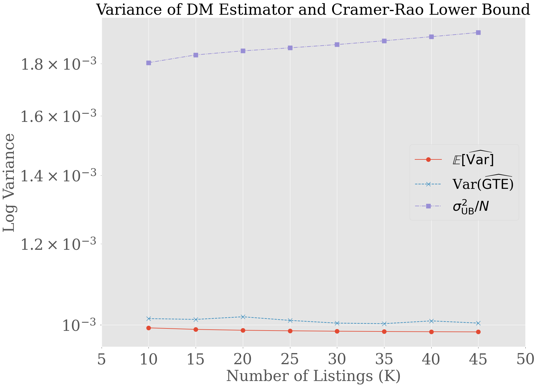
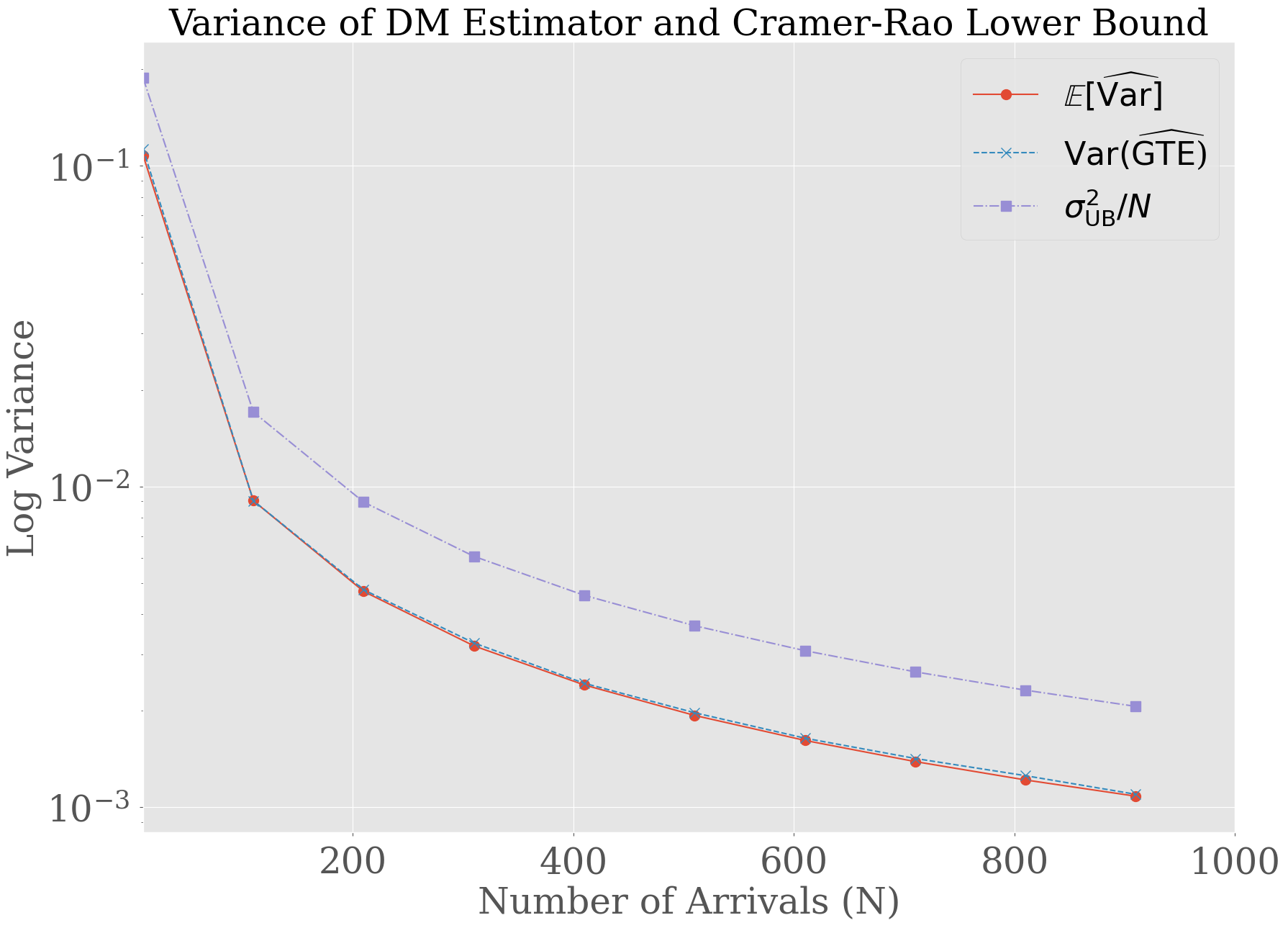
Figure 1: Variance expressions for CR experiments as $K$ (left) and $N$ (right) grow. As both $K$ and $N$ grow, the Cramér-Rao lower bound (and thus the variance of any unbiased estimator) remains larger than the true variance of the DM estimator $\mathrm{Var}(\widehat{\mathsf{GTE}}_{N})$, as well as the estimated variance $\widehat{\mathrm{Var}}$. Parameters are $\lambda=1.5$, $\tau(k)=1$ for all $k$, $a=0.5$ with treatment and control booking probabilities as specified in (26). Error bars are negligible and omitted from the plot.

For the first simulation study, we fix $N=1000$ and let $K$ vary from $10$ to $50$, and we also fix $K=50$ and let $N$ vary from $10$ to $1000$; in Appendix C.2 we vary the other model parameters, and obtain qualitatively similar results. For each value of data point, we compute both the variance of $\widehat{\mathsf{GTE}}_{N}$ and the mean of $\widehat{\mathrm{Var}}_{N}$ over the $5\times 10^{4}$ trajectories, as well as $\sigma^{2}_{\mathsf{UB}}/N$, where $\sigma^{2}_{\mathsf{UB}}$ is the lower bound given in Theorem A.4 in Appendix A.3. The log plot of the variance given in Figure 1 shows that as the number of listings or number of customers grow, the bound $\sigma^{2}_{\mathsf{UB}}/N$ remains larger than the both the true variance of $\widehat{\mathsf{GTE}}_{N}$ and the estimator $\widehat{\mathrm{Var}}_{N}$. This finding, in combination with Theorem 5.2, suggests that the naive test statistic $\hat{T}_{N}$ will have larger power than $\hat{U}_{N}$.

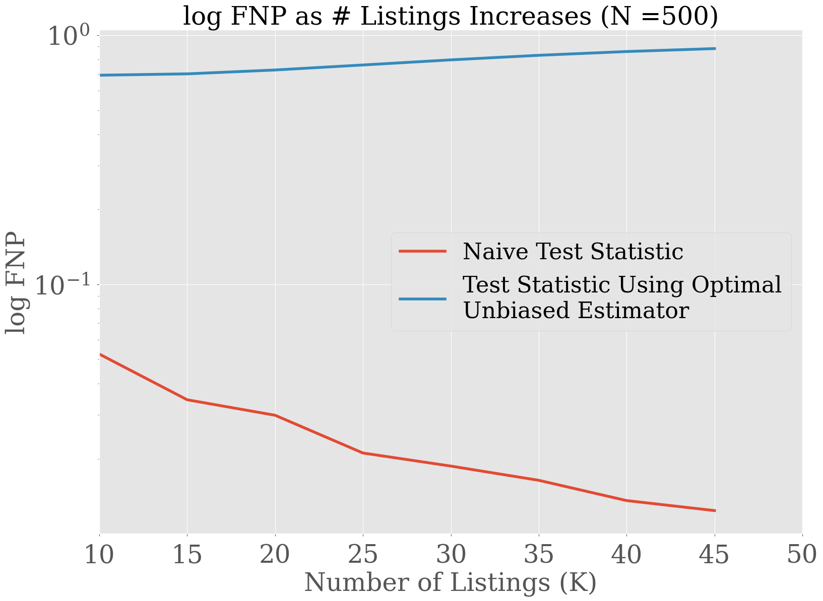
Figure 2: CR experiments with $\lambda=1.5$, $\tau(k)=1$ for all $k$, $a=0.5$, and $K$ (left), $N$ (right) growing. Treatment and control booking probabilities are specified as in (26). For all values of $K$, the log FNP of the test statistic $\hat{T}_{N}$ using the DM estimator $\widehat{\mathsf{GTE}}$ and variance estimator $\widehat{\mathrm{Var}}$ decays faster than the log FNP of an unbiased test statistic (cf. (25)) using an unbiased estimator that obeys (24). Error bars are negligible and omitted from the plot.

For the second simulation study, we fix $K=50$ and let $N$ vary from $10$ to $1000$; in Appendix C.3 we vary other model parameters, and obtain qualitatively similar results. At each data point, we compute the average false negative probability of the naive test statistic $\hat{T}_{N}$ by taking the average number of times the null hypothesis was rejected with significance level $\alpha=0.05$ over the $5*10^{4}$ trajectories. We compare this to the false negative probability ($\mathsf{FNP}$), obtained from the power calculation in (25), for an unbiased estimator $\hat{\theta}_{N}$ that obeys (24). Figure 2 shows the result: the $\mathsf{FNP}$ of $\hat{T}_{N}$ decays faster than $\mathsf{FNP}$ for any such unbiased test statistic, i.e., we obtain higher statistical power using a decision rule with $\hat{T}_{N}$. This matches with the findings of Theorem 5.2 and Figure 1, which suggests that the naive test statistic $\hat{T}_{N}$ should be larger than $\hat{U}_{N}$.

Taken together, these simulation results suggest that the power of the naive test statistic $\hat{T}_{N}$ is actually higher than any test statistic based on an unbiased estimate of the treatment effect, with an associated unbiased variance estimator. This is a striking finding: when combined with Theorem 4.1, we find that the decision maker is uniformly better off not developing a debiased estimator in the presence of interference, when interventions are monotone—they earn the desired control over their false positive probability, and only stand to gain statistical power as a result.

6 Non-monotone treatments

Our analysis thus far has shown that if treatments are monotone, then even without debiasing, a platform is able to control false positive probability (Section  4) while obtaining higher power than any debiased estimation approach (Section  5). In this section, we use simulations to investigate the behavior of false positive probability and statistical power when interventions are non-monotone.

In general, if interventions are non-monotone, it is possible for both quantities to behave arbitrarily worse using the naïve decision-making approach based on the difference-in-means estimator, compared to the decision rule associated to an optimal unbiased estimator. In particular, there exist examples where the false positive probability can become arbitrarily close to 1, instead of being controlled at the desired pre-specified level in the decision rule (15); and there also exist examples where the statistical power remains bounded away from 1, regardless of how many samples are collected—in contrast to the performance of a decision rule that uses an unbiased estimator.

To illustrate these possibilities, we consider a natural class of interventions that are non-monotone, where booking probabilities are increased in lower states (i.e., when many listings are available), and are decreased in larger states (i.e., when few listings are available). These are natural interventions to consider from an operations standpoint. For example, a ridesharing platform may be interested in understanding the impact on rides if prices are lowered relative to the status quo when ample driver supply is available, but raised relative to the status quo when driver supply is relatively tightly constrained.

Concretely, we construct two examples of this form, to illustrate the potential consequences for false positive probability and statistical power, respectively.

Example 6.1.

($\mathsf{ADE}_{a}<0$ but $\mathsf{GTE}=0$.) In the first example, we set $\lambda=1$, $\tau(k)=1$ for each $k$, and $K=30$. We set control booking probabilities $\boldsymbol{\mathrm{p}}_{0}$ as follows:

$$p_{0}(k)=0.5\text{ if }k<K,\text{ }p_{0}(K)=0.$$

(We note in passing that booking probabilities are not strictly decreasing, as in Assumption 3.1, but this is not essential; similar examples can be constructed even if booking probabilities are required to be strictly monotone.) We set treatment booking probabilities as follows:

$$p_{1}(k)=\bar{p}\text{ if }k=0,1;\text{ }p_{1}(k)=0.1\text{ if }2\leq k<K,\text{ }p_{1}(K)=0,$$

where $\bar{p}>0.5$; we show how to choose $\bar{p}$ to ensure that $\mathsf{GTE}=0$. In other words, when the system is nearly empty, the treatment raises booking probabilities relative to control. Otherwise, the treatment lowers booking probabilities relative to control.

To construct $\bar{p}$, we first note that it is straightforward to use the detailed-balance equations to check that a sufficient condition for $\mathsf{GTE}=0$ is:

$$1+\bar{p}+\bar{p}^{2}\frac{1-0.1^{K}}{1-0.1}=\frac{1-0.5^{K}}{1-0.5}.$$

Letting $A_{K}=\frac{1-0.1^{K}}{0.9}$ and $B_{K}=\frac{1-0.5^{K}}{0.5}$, we see that $\bar{p}$ solves

$$A_{K}\bar{p}^{2}+\bar{p}-(B_{K}-1)=0,$$

so in particular we can set

$$\bar{p}=\frac{-1+\sqrt{1+4A_{K}(B_{K}-1)}}{2A_{K}}.$$

For $K=30$, we have $\bar{p}\approx 0.6$, and with these parameters and $a=1/2$ we have $\mathsf{GTE}=0$ yet $\mathsf{ADE}_{a}=-0.009<0$.

We simulate a Bernoulli randomized experiment with $a=1/2$ and $N\in[100,5000]$, with the remaining parameters specified in the previous paragraph. For each fixed set of parameters (ie. fixed $N$), we run $5\times 10^{4}$ trajectories of the experiment, and at each trajectory we form the test statistic (14) using $\widehat{\mathsf{GTE}}$ and $\widehat{\mathrm{Var}}$. We obtain the false positive probability for the naive test statistic by taking the average number of times $H_{0}$ is rejected under significance level $\alpha=0.05$ over the $5\times 10^{4}$ trajectories.

As argued above, the treatments constructed in Example 6.1 produce $\mathsf{ADE}_{a}=-0.009<0$ and $\mathsf{GTE}=0$. As a consequence, this is a treatment where the null hypothesis $H_{0}$ is satisfied. (Note that $\mathsf{GTE}=0$ despite the fact that the treatment and control chains are distinct; this is only possible because the treatment is non-monotone, cf. the discussion in Section  3.5.) However, because $\mathsf{ADE}_{a}<0$, the magnitude of the mean of the test statistic $\hat{T}_{N}$ (cf. (14)) grows without bound. As a consequence, the false positive probability of the test statistic $\hat{T}_{N}$ will increase towards $1$ as $N\to\infty$, as suggested by Figure  3. Of course, a test statistic $\hat{U}_{N}$ using an unbiased estimator for $\mathsf{GTE}$ along with its true variance (cf. (22)) should control the false positive probability correctly, as long as an appropriate central limit theorem holds.

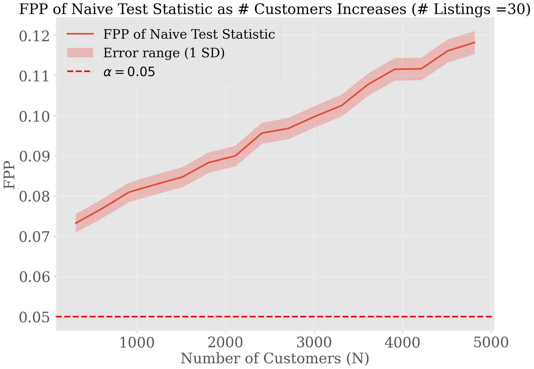
Figure 3: False positive probability of naive test statistic under CR experiment with $a=1/2$ and $N\in[100,5000]$, with $K$, $\lambda$, $\tau(k)$, $\boldsymbol{\mathrm{p}}_{0}$, and $\boldsymbol{\mathrm{p}}_{1}$ specified in Example  6.1. As $N$ grows, the false positive probability grows and will approach $1$.

Example 6.2.

($\mathsf{ADE}_{a}\approx 0$ but $\mathsf{GTE}>0$.) In the second example, we set $\lambda=1$, $\tau(k)=1$, and $K=100$. We set control booking probabilities $\boldsymbol{\mathrm{p}}_{0}$ as follows:

$$p_{0}(k)=0.5\text{ if }k<K;\ p_{0}(K)=0.$$

(Again note that booking probabilities are not strictly decreasing, as in Assumption 3.1, but again, this is not essential.) We set treatment booking probabilities as follows:

$$p_{1}(k)=0.62\text{ if }k=0,1;\ p_{1}(k)=0.07\text{ if }2\leq k<K;p_{1}(K)=0.$$

Again, when the system is nearly empty, the treatment raises booking probabilities relative to control, and otherwise, the treatment lowers booking probabilities relative to control.

We simulate a Bernoulli randomized experiment with $a=1/2$ and $N\in[10,5000]$, with the remaining parameters specified in the previous paragraph. For each fixed set of parameters (ie. fixed $N$), we run $10^{4}$ trajectories of the experiment, and at each trajectory we form the test statistic (14) using $\widehat{\mathsf{GTE}}$ and $\widehat{\mathrm{Var}}$. We obtain the power for the naive test statistic by taking the average number of times $H_{0}$ is rejected under significance level $\alpha=0.05$ over the $5\times 10^{4}$ trajectories.

It is straightforward to verify using the detailed-balance conditions for the global treatment, global control, and experiment birth-death chains (cf. (1)) that in this case $\mathsf{GTE}=0.009$. As a consequence, this is a treatment where the null hypothesis $H_{0}$ is not satisfied. On the other hand, $\mathsf{GTE}\gg\mathsf{ADE}_{a}\approx 0$; in fact, $\mathsf{ADE}_{a}=5.1\times 10^{-8}$. As a consequence, the power under the decision rule (15) is significantly smaller than a test statistic $\hat{U}_{N}$ using an unbiased estimator for $\mathsf{GTE}$ that satisfies (24). This effect is illustrated in Figure  4.

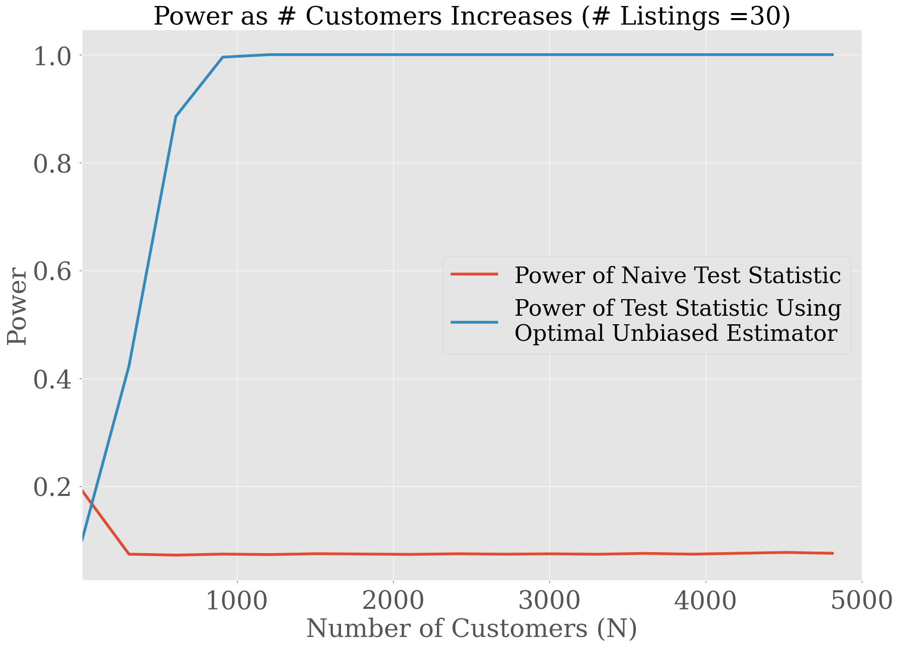
Figure 4: Power of naive test and unbiased test statistic under CR experiment with $a=1/2$, $N\in[10,5000]$,with $K$, $\lambda$, $\tau(k)$, $\boldsymbol{\mathrm{p}}_{0}$, and $\boldsymbol{\mathrm{p}}_{1}$ specified in Example  6.2. As $N$ grows, the power calculation in (25) (for any unbiased estimator that obeys (24)) grows to $1$, while the power of the naive test statistic is much lower.

7 Conclusion

Using a benchmark Markov chain model for a two-sided platform, our results characterize the impact of interference on the false positive probability and statistical power when the experimenter uses naïve estimation based on a t-test statistic. We obtain the surprising finding that when treatments are monotone in a CR experiment, the false positive probability is correctly controlled despite the presence of interference, and that the statistical power is larger than that achieved by using an unbiased estimator. In other words, in this setting the platform is actually better off not using a debiased estimator. Despite these findings, as the simulations in Section 6 suggest, if the treatment is not necessarily monotone then there can be significant gains to false positive probability or statistical power using a debiased estimation method.

Several important directions of work remain. First, our paper considers customer-randomized (CR) experiments; it is natural to also consider whether similar results hold for listing-randomized (LR) experiments [25], where all arriving customers see a mix of treatment and control listings. Given the generality of our results on A/A tests in Section 4.1, we expect that with an appropriate definition of monotone treatments for listing-randomized experiments, similar results as this paper could be obtained.

Second, in our model in Section 3, customers are heterogeneous but listings are homogeneous. It is natural to consider an extension of our model to a setting where listings are heterogeneous as well. (Indeed, development and analysis of LR experiments would require this model extension, to appropriately study a mix of treatment and control listings that are simultaneously in different states of availability.) As for LR experiments, considering listing heterogeneity would also require an appropriate extension of the definition of monotone treatments given in this paper. Interestingly, we conjecture that similar findings as in Section 6 might be obtained in models where listings are heterogeneous, if treatment increases the preference of customers for some types of listings while decreasing their interest in other types of listings. For example, this might be the case if an online labor platform provides the opportunity for workers to display badges and skill certifications on their profile: the resulting change might lead prospective employers to favor certified highly skilled workers over uncertified workers. In such a setting, it would similarly be possible to construct examples where $\mathsf{GTE}=0$ but $\mathsf{ADE}\neq 0$, or $\mathsf{GTE}\neq 0$ but $\mathsf{ADE}=0$—leading to similar qualitative conclusions as our simulations with non-monotone treatments in Section 6.

More broadly, our paper has assumed a particular frequentist hypothesis testing decision-making pipeline, and in particular the use of this pipeline presumes the decision maker cares about type I and type II errors. In practice, there are many reasons this may not be the desired objective, in which case debiasing may be quite valuable. The most obvious such case is when the platform cares about the actual value of $\mathsf{GTE}$ itself; this may be important if launching an intervention carries with it a significant cost, creating a tradeoff for the platform. As an example, a ride-sharing platform may consider the launch of an incentive program for drivers. Even if $\mathsf{GTE}>0$, the platform may only be willing to launch if the cost of supporting such an incentive is not prohibitive relative to the true magnitude of $\mathsf{GTE}$. In this case, debiasing is critical to understand the relative tradeoff between the treatment effect and the cost. A similar situation arises if there are multiple target metrics of interest, and the decision maker faces tradeoffs between the impacts to these objectives.

Indeed, in practice there are a wide range of potential objectives for a platform that uses A/B experimentation. The primary lesson of our work is that the value of debiasing depends on both the desired inferential goal and decision objective, as well as the nature of the treatment itself. Our work serves provides a framework and essential insights for platforms to make choices regarding their inferential and decision-making pipeline in practice.

8 Acknowledgment

This work was supported in part by the National Science Foundation and Stanford Data Science. We are grateful for helpful conversations with Peter Coles, Alex Deng, John Duchi, Inessa Liskovich, Ruben Lobel, Johan Ugander, and Stefan Wager.

Appendix A Experiments on Markov chains

In this self-contained appendix we consider a setting where the treatment and control data generating processes are Markov chains, with rewards also potentially affected by treatment. We provide a central limit theorem for the DM estimator in the setting of general A/B tests, and then specialize our results to A/A tests. Throughout this appendix, $\to^{p}$ denotes convergence in probability; $\Rightarrow$ denotes convergence in distribution; and $\mathcal{N}(m,V)$ denotes a normal random variable with mean $m$ and variance $V$. We conclude by showing that the capacity constrained platform model studied in Section 3 is a special case of this setting.

A.1 Experiments and estimation on general Markov chains

We first present a general model of A/B tests when the data generating processes in treatment and control are Markov chains. We prove a corresponding central limit theorem for $\widehat{\mathsf{GTE}}_{N}$, and also characterize asymptotics of $\widehat{\mathrm{Var}}_{N}$.

State.

We consider homogeneous Markov chains that evolve on a finite state space $S$. We let $X_{1},X_{2},\ldots\in S$ denote the sequence of states visited by the chain.

Bernoulli treatment assignment.

As in the main text, we let $Z_{1},Z_{2},\ldots$ be i.i.d. Bernoulli($a$) random variables, with $0<a<1$.

Markov property and transition probabilities.

At each time step $i$, we consider an order of events where, given the state $X_{i}$ and the treatment assignment $Z_{i}$, the next state $X_{i+1}$ is realized.

Formally, suppose that $X_{1}=x_{1},\ldots,X_{i-1}=x_{i-1},X_{i}=x$, and $Z_{1}=z_{1},\ldots,Z_{i-1}=z_{i-1},Z_{i}=z$. The Markov property asserts that:

$$\mathbb{P}(X_{i+1}=x^{\prime}|X_{i}=x,Z_{i}=z)=\\ \mathbb{P}(X_{i+1}=x^{\prime}|X_{1}=x_{1},\ldots,X_{i-1}=x_{i-1},X_{i}=x;Z_{1}=z_{1},\ldots,Z_{i-1}=z_{i-1},Z_{i}=z).$$

We write $P(x,x^{\prime}|z)=\mathbb{P}(X_{i+1}=x^{\prime}|X_{i}=x,Z_{i}=z)$. Note that this quantity is independent of $i$, so the transition probabilities are stationary in time; in other words, the Markov chain is homogeneous. Note that since treatment assignments are i.i.d. Bernoulli($a$), the sequence $\{X_{i}\}$ is also a discrete-time Markov chain; through an abuse of notation, we represent its transition matrix as $P(\cdot,\cdot|a)$, and we have:

$$P(x,x^{\prime}|a) =a\mathbb{P}(X_{i+1}=x^{\prime}|X_{i}=x,Z_{i}=1)+(1-a)\mathbb{P}(X_{i+1}=x^{\prime}|X_{i}=x,Z_{i}=0)$$

$$=aP(x,x^{\prime}|1)+(1-a)P(x,x^{\prime}|0).$$

We assume for $z=0,1$ that the transition matrix $P(\cdot,\cdot|z)$ is irreducible; therefore for $0<a<1$, $P(\cdot,\cdot|a)$ is also irreducible. Since treatment assignments are i.i.d. Bernoulli($a$), if we let $W_{i}=(X_{i},Z_{i})$, then the Markov chain $\{W_{i}\}$ then has the following transition matrix $R$:

$$R(x,z;x^{\prime},z^{\prime})=\mathbb{P}(X_{i+1}=x^{\prime},Z_{i+1}=z^{\prime}|X_{i}=x,Z_{i}=z)=a^{z^{\prime}}(1-a)^{1-z^{\prime}}P(x,x^{\prime}|z).$$

It then follows that as long as $0<a<1$, the matrix $R$ is irreducible on the state space $S\times\{0,1\}$.

Invariant distribution.

The transition matrix $R$ possesses a unique invariant distribution $\boldsymbol{\mathrm{\nu}}_{a}$. This distribution can be written as follows:

$$\nu_{a}(x,z)=a^{z}(1-a)^{1-z}\pi_{a}(x),$$

where $\pi_{a}(x|z)$ satisfies:

$$\pi_{a}(x)=\sum_{x^{\prime}}\sum_{z^{\prime}=0,1}\nu_{a}(x^{\prime},z^{\prime})P(x^{\prime},x|z^{\prime}).$$

It is straightforward to verify that $\boldsymbol{\mathrm{\pi}}_{a}$ is the invariant distribution of the transition matrix $P(\cdot,\cdot|a)$. We use the subscript $a$ to indicate the treatment fraction. Note that in steady state, the distribution of the state under $\boldsymbol{\mathrm{\nu}}_{a}$ is independent of the treatment assignment; this reflects the fact that treatment assignments are i.i.d.

Throughout our analysis, we write $\mathbb{E}_{\boldsymbol{\mathrm{\nu}}_{a}}$ for expectations when the initial state $(X_{1},Z_{1})$ is sampled from the invariant distribution $\boldsymbol{\mathrm{\nu}}_{a}$. Except in the context of such expectations, we make no assumptions otherwise on the initial state of the chain.

For completeness, for $a=0,1$ we define $\boldsymbol{\mathrm{\pi}}_{0},\boldsymbol{\mathrm{\pi}}_{1}$ to be the invariant distributions of the chain with transition matrix $P(\cdot,\cdot|0)$, $P(\cdot,\cdot|1)$, respectively, i.e., for $a=0,1$, $\pi_{a}(x)=\sum_{x^{\prime}}\pi_{a}(x^{\prime})P(x^{\prime},x|a)$. These are the invariant distributions for global control ($a=0$) and global treatment ($a=1$).

Reward function.

We fix a reward function $g(x,z)$ that depends on the state and treatment indicator, and we let $Y_{i}=g(X_{i},Z_{i})$ for each $i$. Although in principle, rewards may be random given the state, note that we can let $g$ be the expected reward in this case, so our definition is without loss of generality.

Estimand.

The estimand of interest is the steady state difference in reward rate between global treatment and global control, i.e., the global treatment effect:

$$\mathsf{GTE}=\sum_{x}\pi_{1}(x)g(x,1)-\sum_{x}\pi_{0}(x)g(x,0).$$ (28)

Difference-in-means (DM) estimator and variance estimator.

Both $\widehat{\mathsf{GTE}}_{N}$ and $\widehat{\mathrm{Var}}_{N}$ are defined identically to the main text, cf. (5) and (6). As we consider only asymptotic results as $N\to\infty$ in our analysis in this section, we implicitly condition all our analysis on the (almost sure) event that $N_{1N}>0$ and $N_{0N}>N$.

Central limit theorem.

We now state a central limit theorem for the difference-in-means estimator. To state the theorem, we require some additional notation. First define:

$$\mathsf{ADE}_{a}=\sum_{x}\pi_{a}(x)g(x,1)-\sum_{x}\pi_{a}(x)g(x,0).$$

The quantity $\mathsf{ADE}_{a}$ is the average direct effect [18]. Since, in general, this steady state distribution neither matches global treatment nor global control, in general $\mathsf{ADE}_{a}\neq\mathsf{GTE}$.

Next, define the following quantities for $z,z^{\prime}\in\{0,1\}$:

$$V(z) =\mathbb{E}_{\boldsymbol{\mathrm{\nu}}_{a}}\left[\left(g(X_{1},z)-\sum_{x}\pi_{a}(x)g(x,z)\right)^{2}\Bigg{|}Z_{1}=z\right]$$

$$=\sum_{x}\pi_{a}(x)\left(g(x,z)-\sum_{x^{\prime}}\pi_{a}(x^{\prime})g(x^{\prime},z)\right)^{2}$$

$$=\mathrm{Var}_{\boldsymbol{\mathrm{\nu}}_{a}}(Y_{1}|Z_{1}=z);$$

$$C_{j}(z,z^{\prime}) =\mathbb{E}_{\boldsymbol{\mathrm{\nu}}_{a}}\left[\left(g(X_{1},z)-\sum_{x}\pi_{a}(x)g(x,z)\right)\left(g(X_{j},z^{\prime})-\sum_{x}\pi_{a}(x)g(x,z^{\prime})\right)\Bigg{|}Z_{1}=z,Z_{j}=z^{\prime}\right]$$

$$=\mathrm{Cov}_{\boldsymbol{\mathrm{\nu}}_{a}}(Y_{1},Y_{j}|Z_{1}=z,Z_{j}=z^{\prime}),$$

where we recall that $Y_{i}=g(X_{i},Z_{i})$. These quantities capture the conditional variance and covariance of rewards, respectively, given treatment assignments. Observe that although the expectations are with respect to the steady state distribution of $\{W_{t}\}$, i.e., $\boldsymbol{\mathrm{\nu}}_{a}$, in fact $V(z)$ can be reduced to an expectation against the steady state distribution of $\{X_{t}\}$, i.e., $\boldsymbol{\mathrm{\pi}}_{a}$. This is because the expectation only involves $X_{1}$, which is independent of $Z_{1}$. The same is true for $X_{1}$ in the definition of $C_{j}(z,z^{\prime})$; however, $X_{j}$ in the definition of $C_{j}$ does depend on the initial treatment assignment $Z_{1}$.

We have the following theorem. The proof combines a standard Markov central limit theorem (e.g., [26], Theorem 1) with techniques for the central limit theorem of the difference-in-means estimator with i.i.d. observations (e.g., [49], Theorem 1.2).

Theorem A.1.

Suppose $0<a<1$. Then regardless of the initial distribution, $\widehat{\mathsf{GTE}}_{N}\to^{p}\mathsf{ADE}_{a}$ as $N\to\infty$, and $\widehat{\mathsf{GTE}}_{N}$ obeys the following central limit theorem as $N\to\infty$:

$$\sqrt{N}(\widehat{\mathsf{GTE}}_{N}-\mathsf{ADE}_{a})\Rightarrow\mathcal{N}\left(0,\tilde{\sigma}_{a}^{2}\right),$$ (29)

where:

$$\tilde{\sigma}_{a}^{2}=\left(\frac{1}{1-a}\right)V(0)+\left(\frac{1}{a}\right)V(1)+2\sum_{j>1}C_{j}(0,0)+C_{j}(1,1)-C_{j}(0,1)-C_{j}(1,0),$$ (30)

with $\tilde{\sigma}_{a}^{2}>0$.

Proof.

We first prove the convergence in probability of $\widehat{\mathsf{GTE}}_{N}$. Note that $N(1-a)/N_{0N}\to^{p}1$, and $Na/N_{1N}\to^{p}1$. Thus the ergodic theorem for Markov chains establishes that:

$$\overline{Y}(0)\to^{p}\left(\frac{1}{1-a}\right)\mathbb{E}_{\boldsymbol{\mathrm{\nu}}_{a}}[(1-Z_{1})Y_{1}];\ \ \overline{Y}(1)\to^{p}\left(\frac{1}{a}\right)\mathbb{E}_{\boldsymbol{\mathrm{\nu}}_{a}}[Z_{1}Y_{1}].$$

Note that:

$$\mathbb{E}_{\boldsymbol{\mathrm{\nu}}_{a}}[(1-Z_{1})Y_{1}]=(1-a)\mathbb{E}_{\boldsymbol{\mathrm{\nu}}_{a}}[g(X_{1},0)|Z_{1}=0]=(1-a)\sum_{x}\pi_{a}(x)g(x,0);$$

similarly, $\mathbb{E}_{\boldsymbol{\mathrm{\nu}}_{a}}[Z_{1}Y_{1}]=a\sum_{x}\pi_{a}(x)g(x,1)$. We conclude that:

$$\overline{Y}(0)\to^{p}\sum_{x}\pi_{a}(x)g(x,0);\ \ \overline{Y}(1)\to^{p}\sum_{x}\pi_{a}(x)g(x,1),$$ (31)

so that $\widehat{\mathsf{GTE}}_{N}\to^{p}\mathsf{ADE}_{a}$ as $N\to\infty$.

For $z\in\{0,1\}$ and $x\in S$, define:

$$h_{1}(x,z) =\left(\frac{z}{a}\right)\left(g(x,1)-\sum_{x^{\prime}}\pi_{a}(x^{\prime})g(x^{\prime},1)\right);$$

$$h_{0}(x,z) =\left(\frac{1-z}{1-a}\right)\left(g(x,0)-\sum_{x^{\prime}}\pi_{a}(x^{\prime})g(x^{\prime},0)\right).$$

Observe that $h_{1}(x,0)=h_{0}(x,1)=0$. Further, observe that:

$$\mathbb{E}_{\boldsymbol{\mathrm{\nu}}_{a}}[h_{1}(W_{1})]=a\mathbb{E}_{\boldsymbol{\mathrm{\nu}}_{a}}[h_{1}(X_{1},1)|Z_{1}=1]=\mathbb{E}_{\boldsymbol{\mathrm{\nu}}_{a}}[g(X_{1},1)|Z_{1}=1]-\sum_{x}\pi_{a}(x)g(x,1)=0;$$

similarly, $\mathbb{E}_{\boldsymbol{\mathrm{\nu}}_{a}}[h_{0}(W_{1})]=0$.

For fixed, arbitrary $t_{0},t_{1}\in\mathbb{R}$, define $h(z,x)=t_{0}h_{0}(x,z)+t_{1}h_{1}(x,z)$. Since $\mathbb{E}_{\boldsymbol{\mathrm{\nu}}_{a}}[h_{1}(W_{1})]=\mathbb{E}_{\boldsymbol{\mathrm{\nu}}_{a}}[h_{0}(W_{1})]=0$, we have $\mathbb{E}_{\boldsymbol{\mathrm{\nu}}_{a}}[h(W_{1})]=0$ as well.

The standard central limit theorem for Markov chains (see, e.g., [26], Theorem 1) thus implies that:

$$\frac{1}{\sqrt{N}}\sum_{i=1}^{N}h(W_{i})\Rightarrow\mathcal{N}(0,\gamma(t_{0},t_{1})^{2}),$$

where:

$$\gamma(t_{0},t_{1})^{2}=\mathbb{E}_{\boldsymbol{\mathrm{\nu}}_{a}}[h(W_{1})^{2}]+2\sum_{j>1}\mathbb{E}_{\boldsymbol{\mathrm{\nu}}_{a}}[h(W_{1})h(W_{j})].$$

Straightforward algebra gives the following identities:

$$\mathbb{E}_{\boldsymbol{\mathrm{\nu}}_{a}}[h(W_{1})^{2}] =t_{0}^{2}\mathbb{E}_{\boldsymbol{\mathrm{\nu}}_{a}}[h_{0}(W_{1})^{2}]+t_{1}^{2}\mathbb{E}_{\boldsymbol{\mathrm{\nu}}_{a}}[h_{1}(W_{1})^{2}]$$

$$\ \ +2t_{0}t_{1}\mathbb{E}_{\boldsymbol{\mathrm{\nu}}_{a}}[h_{0}(W_{1})h_{1}(W_{1})];$$

$$\mathbb{E}_{\boldsymbol{\mathrm{\nu}}_{a}}[h(W_{1})h(W_{j})] =t_{0}^{2}\mathbb{E}_{\boldsymbol{\mathrm{\nu}}_{a}}[h_{0}(W_{1})h_{0}(W_{j})]+t_{1}^{2}\mathbb{E}_{\boldsymbol{\mathrm{\nu}}_{a}}[h_{1}(W_{1})h_{1}(W_{j})]$$

$$\ \ +t_{0}t_{1}\mathbb{E}_{\boldsymbol{\mathrm{\nu}}_{a}}[h_{0}(W_{1})h_{1}(W_{j})+h_{1}(W_{1})h_{0}(W_{j})].$$

Observe that for any realization of $W_{1}=(X_{1},Z_{1})$, we have $h_{0}(W_{1})h_{1}(W_{1})=0$, since either $Z_{1}=0$ or $1-Z_{1}=0$. Further, observe that by conditioning on the realization of $Z_{1}$, we have:

$$\mathbb{E}_{\boldsymbol{\mathrm{\nu}}_{a}}[h_{0}(W_{1})^{2}] =\mathbb{E}_{\boldsymbol{\mathrm{\nu}}_{a}}\left[\left(\frac{1-Z_{1}}{1-a}\right)^{2}\left(g(X_{1},0)-\sum_{x}\pi_{a}(x)g(x,0)\right)^{2}\right]$$

$$=\left(\frac{1}{1-a}\right)\mathbb{E}_{\boldsymbol{\mathrm{\nu}}_{a}}\left[\left(g(X_{1},0)-\sum_{x}\pi_{a}(x)g(x,0)\right)^{2}\Bigg{|}Z_{1}=0\right]$$

$$=\left(\frac{1}{1-a}\right)V(0).$$

Similarly, we have:

$$\mathbb{E}_{\boldsymbol{\mathrm{\nu}}_{a}}[h_{0}(W_{1})h_{0}(W_{j})] =\mathbb{E}_{\boldsymbol{\mathrm{\nu}}_{a}}\Bigg{[}\left(\frac{(1-Z_{1})(1-Z_{j})}{(1-a)^{2}}\right)$$

$$\qquad\qquad\cdot\left(g(X_{1},0)-\sum_{x}\pi_{a}(x)g(x,0)\right)\left(g(X_{j},0)-\sum_{x}\pi_{a}(x)g(x,0)\right)\Bigg{]}$$

$$=\mathbb{E}_{\boldsymbol{\mathrm{\nu}}_{a}}\left[\left(g(X_{1},0)-\sum_{x}\pi_{a}(x)g(x,0)\right)\left(g(X_{j},0)-\sum_{x}\pi_{a}(x)g(x,0)\right)\Bigg{|}Z_{1}=0,Z_{j}=0\right]$$

$$=C_{j}(0,0).$$

Using similar arguments, we arrive at the following identities:

$$\mathbb{E}_{\boldsymbol{\mathrm{\nu}}_{a}}[h(W_{1})^{2}] =\left(\frac{t_{0}^{2}}{1-a}\right)V(0)+\left(\frac{t_{1}^{2}}{a}\right)V(1);$$

$$\mathbb{E}_{\boldsymbol{\mathrm{\nu}}_{a}}[h(W_{1})h(W_{j})] =t_{0}^{2}C_{j}(0,0)+t_{1}^{2}C_{j}(1,1)+t_{0}t_{1}(C_{j}(0,1)+C_{j}(1,0)).$$

Now let $(U_{0},U_{1})$ be a jointly normally distributed random pair, with mean zero, and covariance matrix:

$$\boldsymbol{\mathrm{\Sigma}}=\left(\begin{array}[]{cc}V(0)/(1-a)+2\sum_{j>1}C_{j}(0,0)&\sum_{j>1}C_{j}(0,1)+C_{j}(1,0)\\ \sum_{j>1}C_{j}(0,1)+C_{j}(1,0)&V(1)/a+2\sum_{j>1}C_{j}(1,1)\end{array}\right).$$

We have shown that:

$$t_{0}\left(\frac{1}{\sqrt{N}}\sum_{i=1}^{N}h_{0}(W_{i})\right)+t_{1}\left(\frac{1}{\sqrt{N}}\sum_{i=1}^{N}h_{1}(W_{i})\right)\Rightarrow t_{0}U_{0}+t_{1}U_{1}.$$

Using the Cramér-Wold device, we conclude that:

$$\left(\frac{1}{\sqrt{N}}\sum_{i=1}^{N}h_{0}(W_{i}),\frac{1}{\sqrt{N}}\sum_{i=1}^{N}h_{1}(W_{i})\right)\Rightarrow\mathcal{N}(\boldsymbol{\mathrm{0}},\boldsymbol{\mathrm{\Sigma}}).$$

Define:

$$\boldsymbol{\mathrm{\Gamma}}_{N}=\left(\begin{array}[]{c}\frac{(N(1-a))}{N_{0N}}\cdot\frac{1}{N}\sum_{i=1}^{N}h_{0}(W_{i})\\ \frac{Na}{N_{1N}}\cdot\frac{1}{N}\sum_{i=1}^{N}h_{1}(W_{i})\end{array}\right)=\left(\begin{array}[]{c}\frac{1}{N_{0N}}\sum_{i=1}^{N}(1-Z_{i})\left(g(X_{i},0)-\sum_{x^{\prime}}\pi_{a}(x^{\prime})g(x^{\prime},0)\right)\\ \frac{1}{N_{1N}}\sum_{i=1}^{N}Z_{i}\left(g(X_{i},1)-\sum_{x^{\prime}}\pi_{a}(x^{\prime})g(x^{\prime},1)\right)\end{array}\right).$$

Since $N(1-a)/N_{0N}\to^{p}1$, and $Na/N_{1N}\to^{p}1$, by Slutsky’s theorem we have:

$$\sqrt{N}\boldsymbol{\mathrm{\Gamma}}_{N}\Rightarrow\mathcal{N}(\boldsymbol{\mathrm{0}},\boldsymbol{\mathrm{\Sigma}}).$$

Now observe that:

$$(-1,1)^{\top}\boldsymbol{\mathrm{\Gamma}}_{N} =\frac{1}{N_{1N}}\sum_{i=1}^{N}Z_{i}g(X_{i},1)-\frac{1}{N_{0N}}\sum_{i=1}^{N}(1-Z_{i})g(X_{i},0)$$

$$\ \ -\left(\sum_{x^{\prime}}\pi_{a}(x^{\prime})g(x^{\prime},1)-\sum_{x^{\prime}}\pi_{a}(x^{\prime})g(x^{\prime},0)\right)$$

$$=\widehat{\mathsf{GTE}}_{N}-\mathsf{ADE}_{a},$$

since $Z_{i}g(X_{i},1)=Z_{i}Y_{i}$ and $(1-Z_{i})g(X_{i},0)=(1-Z_{i})Y_{i}$. Straightforward algebra shows that $\tilde{\sigma}^{2}=(-1,1)^{\top}\Sigma(-1,1)$. Thus we have shown (29). ∎

Limit of variance estimator.

The following theorem gives the scaled limit of $\widehat{\mathrm{Var}}$.

Theorem A.2.

Suppose $0<a<1$. Then $\widehat{\mathrm{Var}}_{N}$ satisfies

$$N\widehat{\mathrm{Var}}_{N}\to^{p}\left(\frac{1}{a}\right)V(1)+\left(\frac{1}{1-a}\right)V(0).$$ (32)

Note that in comparison to the true variance $\tilde{\sigma}^{2}$, the estimator misses all the covariance terms. Whether this is an overestimate or underestimate of the true variance depends on whether the within-group covariances are stronger are weaker than the across-group covariances, cf. (30).

Proof.

We observe using a standard calculation that:

$$\sum_{i=1}^{N}Z_{i}(Y_{i}-\overline{Y}(1))^{2}=\sum_{i=1}^{N}Z_{i}Y_{i}^{2}-N_{1N}\overline{Y}(1)^{2}.$$

From (31), we know that $\overline{Y}(1)\to^{p}\sum_{x}\pi_{a}(x)g(x,1).$ We know $N_{1N}/(Na)\to^{p}1$ as $N\to\infty$, so by the ergodic theorem, we have:

$$\frac{1}{N_{1N}}\sum_{i=1}^{N}Z_{i}Y_{i}^{2}\to^{p}\frac{1}{a}\mathbb{E}_{\boldsymbol{\mathrm{\nu}}_{a}}[Z_{1}Y_{1}^{2}].$$

We have:

$$\mathbb{E}_{\boldsymbol{\mathrm{\nu}}_{a}}[Z_{1}Y_{1}^{2}]=a\mathbb{E}_{\boldsymbol{\mathrm{\nu}}_{a}}[g(X_{1},1)^{2}|Z_{1}=1]=a\sum_{x}\pi_{a}(x)g(x,1)^{2}.$$

Finally, note that $N/(N_{1N}-1)\to^{p}1/a$ as $N\to\infty$ as well. Combining all these facts, we conclude that:

$$\frac{N}{(N_{1N}-1)N_{1N}}\sum_{i=1}^{N}Z_{i}(Y_{i}-\overline{Y}(1))^{2}\to^{p}\frac{1}{a}V(1).$$

An analogous calculation follows for the second term of $\widehat{\mathrm{Var}}_{N}$, establishing the claimed convergence of $N\widehat{\mathrm{Var}}_{N}$. ∎

Note that the preceding result implies the t-test statistic centered at $\mathsf{ADE}_{N}$ given by $(\widehat{\mathsf{GTE}}_{N}-\mathsf{ADE}_{N})/\sqrt{\widehat{\mathrm{Var}}_{N}}$ converges in distribution to a normal random variable with zero mean, and variance:

$$\frac{V(0)/(1-a)+V(1)/a)}{V(0)/(1-a)+V(1)/a+2\sum_{j>1}C_{j}(0,0)+C_{j}(1,1)-C_{j}(0,1)-C_{j}(1,0).}$$

A.2 A/A experiments of Markov chains

In this section, we apply our preceding results to A/A experiments in a Markov chain setting. These are experiments where both the treatment and control chains are identical, the treatment assignment is completely independent of the Markov chain evolution; and where the rewards do not depend on treatment assignment. See also Section 4.1 for further discussion of A/A experiments.

Formally, we suppose that that there is a single irreducible transition matrix $P$ such that $P(x,x^{\prime}|0)=P(x,x^{\prime}|1)=P$; let $\boldsymbol{\mathrm{\pi}}$ be the invariant distribution of this matrix. This makes the evolution of $\{X_{i}\}$ independent of the realization of the treatment assignments $\{Z_{i}\}$. It follows that for all $a$, $0\leq a\leq 1$, we have $\boldsymbol{\mathrm{\pi}}_{a}=\boldsymbol{\mathrm{\pi}}$; and thus:

$$\nu_{a}(x,z)=a^{z}(1-a)^{1-z}\pi(x).$$

We also assume that there is a single reward function $g$ such that $g(x,0)=g(x,1)=g(x)$. Note that the resulting reward sequence $\{Y_{i}\}$ with $Y_{i}=g(X_{i})$ is thus also independent of $\{Z_{i}\}$.

It follows from these definitions that for an A/A test, $\mathsf{GTE}=\mathsf{ADE}_{a}=0$. We note also that with these definitions, we have:

$$V=V(0)=V(1)=\sum_{x}\pi(x)\left(g(x)-\sum_{x^{\prime}}\pi(x^{\prime})g(x^{\prime})\right)^{2}.$$ (33)

Further, since all treatment assignments are independent of the states $(X_{1},X_{j})$, we have:

$$C_{j} =C_{j}(0,0)=C_{j}(1,1)=C_{j}(0,1)=C_{j}(1,0)$$

$$=\mathbb{E}_{\boldsymbol{\mathrm{\pi}}}\left[\left(g(X_{1})-\sum_{x}\pi(x)g(x)\right)\left(g(X_{j})-\sum_{x}\pi(x)g(x)\right)\right],$$

where the notation $\mathbb{E}_{\boldsymbol{\mathrm{\pi}}}$ denotes that we take expectations with respect to the chain where the initial state $X_{1}$ is sampled from $\boldsymbol{\mathrm{\pi}}$. Combining Theorems A.1 and A.2 with these observations, we have the following result.

Theorem A.3.

Suppose $0<a<1$. For an A/A experiment, $\widehat{\mathsf{GTE}}_{N}$ obeys the following central limit theorem as $N\to\infty$:

$$\sqrt{N}\widehat{\mathsf{GTE}}_{N}\Rightarrow\mathcal{N}\left(0,\left(\frac{1}{a}+\frac{1}{1-a}\right)V\right)$$ (34)

where $V$ is defined as in (33). In addition, $\widehat{\mathrm{Var}}_{N}$ satisfies

$$N\widehat{\mathrm{Var}}_{N}\to^{p}\left(\frac{1}{a}+\frac{1}{1-a}\right)V.$$ (35)

In particular, the t-test statistic converges in distribution to a standard normal random variable:

$$\frac{\widehat{\mathsf{GTE}}_{N}}{\sqrt{\widehat{\mathrm{Var}}_{N}}}\Rightarrow\mathcal{N}(0,1).$$

This result, when applied to general A/A tests in a Markov chain environment, can be used to demonstrate control of the false positive probability. In particular, suppose for each $N$ that the null hypothesis $\tilde{H}_{0}$ is defined as in (18), i.e., the null hypothesis assumes that the observations $Y_{1},\ldots,Y_{N}$ are independent of $Z_{1},\ldots,Z_{N}$. Further suppose the test statistic $\hat{T}_{N}$ is defined as in (14), and the decision rule (15) with the null hypothesis is $\tilde{H}_{0}$ is followed.

The corresponding false positive probability is the chance that $\tilde{H}_{0}$ is mistakenly rejected when it is true. Formally, this is:

$$\mathsf{FPP}_{N}=\mathbb{P}(\hat{T}_{N}>\Phi_{\alpha/2}|\tilde{H}_{0}),$$ (36)

where the distribution of observations comes from the Markov chain and rewards defined by $P$ and $g$ respectively, with a fixed initial distribution. Note that $\mathsf{FPP}_{N}$ in (36) is well defined: Given that $Y_{1},\ldots,Y_{N}$ are generated in this way, and $Z_{1},\ldots,Z_{N}$ are i.i.d., as well as independent of $Y_{1},\ldots,Y_{N}$ under $\tilde{H}_{0}$, the distribution of $\hat{T}_{N}$ is completely determined.

Theorem A.3 then implies the following corollary.

Corollary A.1.

Suppose $0<a<1$. Then for an A/A experiment, as $N\to\infty$, $\mathsf{FPP}_{N}\to\alpha$, where $\mathsf{FPP}_{N}$ is defined as in (36).

The preceding result shows that for general A/A experiments in Markov chain environments, the false positive probability of the decision rule (15) is (asymptotically) controlled at level $\alpha$, as intended.

A.3 Cramér-Rao bound for A/B experiments of Markov chains

In this section we present a result of [11], which uses the multivariate Cramér-Rao bound to provide a lower bound on the s variance of any unbiased $\mathsf{GTE}$ estimator for an A/B experiment between two Markov chains. The same paper provides a least squares temporal difference (LSTD)-based unbiased estimator that matches this lower bound. (A similar variance calculation is obtained via a nonparametric maximum likelihood design and estimation approach in [14].)

As in Section 5.2, in the general Markov chain setting we consider here, an estimator $\hat{\theta}_{N}$ is a real-valued functional of the observations $Y_{1},\ldots,Y_{N}$ generated from a Bernoulli randomized experiment. We say that $\hat{\theta}_{N}$ is an unbiased estimator if for all feasible values of system parameters (i.e., $S$, $P$, $g$) and the design parameter $a$, there holds $\mathbb{E}[\hat{\theta}_{N}]=\mathsf{GTE}$, where $\mathsf{GTE}$ is defined as in (28).

Theorem A.4 ([11]).

Let $\hat{\theta}_{N}$ be an unbiased estimator for $\mathsf{GTE}$ for all feasible values of system parameters (i.e., $S$, $P$, $g$) and the design parameter $a$. Then $\mathrm{Var}(\hat{\theta}_{N})$ satisfies

$$N\mathrm{Var}(\hat{\theta}_{N})\geq\frac{1}{a}\sum_{x,x^{\prime}}\frac{\pi_{1}(x)^{2}}{\nu_{a}(x,1)}P(x,x^{\prime}|1)(v(x^{\prime}|1)-v(x|1)+g(x,1))^{2}$$

$$+\frac{1}{1-a}\sum_{x,x^{\prime}}\frac{\pi_{0}(x)^{2}}{\nu_{a}(x,0)}P(x,x^{\prime}|0)(v(x^{\prime}|0)-v(x|0)+g(x,0))^{2}:=\sigma^{2}_{\mathsf{UB}}.$$

where:

$$v(x|z)=\mathbb{E}\left[\sum_{t=1}^{\infty}\left(g(X_{t},Z_{t})-\sum_{x^{\prime}}\pi_{z}(x^{\prime})g(x^{\prime},z)\right)\ \Bigg{|}\ X_{0}=x,Z_{t}=z\ \text{for all}\ t\right].$$

In the preceding statement, $v(x|z)$ is the value function of either the global treatment condition (if $z=1$) or the global control condition (if $z=0$); the quantity $v(x|z)$ measures the cumulative difference between realized rewards and the average reward per time step.

A.4 Application to a capacity-constrained platform

In this section we show that the model in Section 3 is a special case of the general Markov chain setting presented here, and can be analyzed using the same limit theorems.

To make the mapping, we must define appropriate discrete time Markov chains corresponding to global treatment and global control, and a corresponding reward function $g$. We proceed as follows. Following Section 3, let $X_{t}$ is the continuous time Markov chain of booked listings under global treatment (i.e., $a=1$). Let $T(i)$ be the arrival time of the $i$’th customer, and let $X_{T(i)}^{-}$ denote the state just before the arrival of the $i$’th customer. Let $S_{i}=(X_{T(i)}^{-},Y_{i})$. Note that $S_{i}$ is a stationary discrete-time Markov chain on the finite state space $\{0,\ldots,K\}\times\{0,1\}$: given $S_{i}$, the next state $X_{T(i+1)}^{-}$ is independent of the history prior to customer $i$, and of course given $X_{T(i+1)}^{-}$, the booking outcome $Y_{i+1}$ of customer $i+1$ is also independent of the history prior customer $i$.

We let $P(k,y,k^{\prime},y^{\prime}|1)$ be the transition matrix of this discrete-time Markov chain corresponding to global treatment. Note that since Poisson arrivals see time averages (PASTA), the steady state distribution of $P(\cdot|1)$ is:

$$\phi_{1}(k,y)=\pi_{1}(k)p_{1}(k).$$

We can similarly define $P(k,y,k^{\prime},y^{\prime}|0)$ for the global control chain, with an analogous steady state distribution $\phi_{0}(k,y)$.

Finally, for each state $k$, $y=0,1$, and $z=0,1$, define the reward function $g(k,y,z)=y$; this is the booking outcome. Note the difference in long run average reward between the treatment and control chains is:

$$\sum_{k}\sum_{y=0,1}\phi_{1}(k,y)g(k,y)-\sum_{k}\sum_{y=0,1}\phi_{0}(k,y)g(k,y)=\sum_{k}\pi_{1}(k)p_{1}(k)-\sum_{k}\pi_{0}(k)p_{0}(k)=\mathsf{GTE},$$

i.e., exactly the global treatment effect defined in (4). Thus the estimand in Section 3 is exactly the estimand in (28), i.e., the difference in long run average reward between the treatment and control discrete time chains with the primitives $P(\cdot|1)$, $P(\cdot|0)$, and $g$ defined as in this section.

Thus Theorems A.1 and A.2 directly apply in the setting of Section 3, with the primitives defined as in this section. Applications of these results with the specific primitives defined above yields Theorems 3.1 and 3.2 in the main text. Application of Theorem A.4 yields the Cramér-Rao bound we leverage in Section 5.2, and in particular (23).

We remark here that it is important to carefully translate the expectations in the variances and covariances that appear in Theorem A.1. These are expectations evaluated with the initial distribution of the discrete-time chain initialized to $\boldsymbol{\mathrm{\pi}}_{1}$ or $\boldsymbol{\mathrm{\pi}}_{0}$ for global treatment and global control, respectively. In the continuous time Markov chain of Section 3, this corresponds to the requirement that the distribution of the state just prior to the arrival of the first customer is the steady state distribution $\boldsymbol{\mathrm{\pi}}_{1}$ or $\boldsymbol{\mathrm{\pi}}_{0}$.

Finally, observe that if the null hypothesis $H_{0}:\mathsf{GTE}=0$ holds and the treatment is monotone, then by Proposition 3.1 we know that $p_{0}=p_{1}$, i.e., we are in the setting of an A/A experiment: both treatment and control Markov chains are identical. Theorem 4.1 in the main text then follows by applying Theorem A.3 and Corollary A.1 to the resulting A/A experiment.

Appendix B Additional proofs

Proof of Proposition 3.1.

Clearly if $\boldsymbol{\mathrm{p}}_{1}=\boldsymbol{\mathrm{p}}_{0}$ then $\mathsf{GTE}=0.$ Now suppose $\boldsymbol{\mathrm{p}}_{1}\neq\boldsymbol{\mathrm{p}}_{0}$, i.e., for at least one $k$, $p_{1}(k)\neq p_{0}(k)$. Under Assumption 3.2, we either have $p_{1}(k)\geq p_{0}(k)$ for all $k$ or $p_{1}(k)\leq p_{0}(k)$ for all $k$; and since $\boldsymbol{\mathrm{p}}_{1}\neq\boldsymbol{\mathrm{p}}_{0}$, we have strict inequality for at least one $k$. We focus on the case where $p_{1}(k)\geq p_{0}(k)$ for all $k$, since the opposite case is symmetric. If $p_{1}(k)\geq p_{0}(k)$ for all $k$ and $\boldsymbol{\mathrm{p}}_{0}\neq\boldsymbol{\mathrm{p}}_{1}$ (i.e., a strictly positive treatment), then $\boldsymbol{\mathrm{\pi}}_{1}\succ^{d}\boldsymbol{\mathrm{\pi}}_{0}$, cf. Definition 5.1 and Corollary 5.1.

Now observe that since $\boldsymbol{\mathrm{p}}_{1}$ is strictly decreasing, cf. Assumption 3.1, and $\boldsymbol{\mathrm{\pi}}_{1}\succ^{d}\boldsymbol{\mathrm{\pi}}_{0}$, we conclude:

$$\rho_{1}=\sum_{k}\pi_{1}(k)p_{1}(k)>\sum_{k}\pi_{0}(k)p_{1}(k).$$

Further, since $p_{1}(k)\geq p_{0}(k)$ for all $k$ with strict inequality for at least one $k$, we have:

$$\sum_{k}\pi_{0}(k)p_{1}(k)>\sum_{k}\pi_{0}(k)p_{0}(k)=\rho_{0}.$$

Thus $\rho_{1}>\rho_{0}$. Since $\mathsf{GTE}=\rho_{1}-\rho_{0}$, we must have $\mathsf{GTE}>0$. On the other hand, if $p_{1}(k)\leq p_{0}(k)$ for all $k$ and $\boldsymbol{\mathrm{p}}_{1}\neq\boldsymbol{\mathrm{p}}_{0}$, then we have $\boldsymbol{\mathrm{\pi}}_{1}\prec^{d}\boldsymbol{\mathrm{\pi}}_{0}$. A symmetric argument then yields $\rho_{0}>\rho_{1}$, and we would conclude $\mathsf{GTE}<0.$ In either case, we have shown that $\boldsymbol{\mathrm{p}}_{1}\neq\boldsymbol{\mathrm{p}}_{0}$ implies $\mathsf{GTE}\neq 0.$ ∎

Proof of Proposition 4.3.

We condition on the realization of $\boldsymbol{\mathrm{Z}}$. We have:

$$\mathrm{Var}(\widehat{\mathsf{GTE}}|\boldsymbol{\mathrm{Z}}) =\frac{1}{N_{1}^{2}}(N_{1}V+N_{1}(N_{1}-1)C)+\frac{1}{N_{0}^{2}}(N_{0}V+N_{0}(N_{0}-1)C))-\frac{1}{N_{1}N_{0}}(2N_{1}N_{0}C)$$

$$=\left(\frac{1}{N_{1}}+\frac{1}{N_{0}}\right)(V-C).$$ (37)

Next we compute the expected value of the variance estimator $\widehat{\mathrm{Var}}$. We again do this by first conditioning on the realization of the $\boldsymbol{\mathrm{Z}}$ vector. Straightforward manipulation gives:

$$\widehat{\mathrm{Var}}=\frac{1}{N_{1}(N_{1}-1)}\sum_{i}Z_{i}(Y_{i}^{2}-\overline{Y}(1)^{2})+\frac{1}{N_{0}(N_{0}-1)}\sum_{i}(1-Z_{i})(Y_{i}^{2}-\overline{Y}(0)^{2}).$$

We consider the first term, since the analysis for the second is identical. We have:

$$\mathbb{E}\left[\overline{Y}(1)^{2}|\boldsymbol{\mathrm{Z}}\right] =\frac{1}{N_{1}^{2}}\mathbb{E}\left[\left(\sum_{i}Z_{i}Y_{i}\right)^{2}\Bigg{|}\boldsymbol{\mathrm{Z}}\right]$$

$$=\frac{1}{N_{1}^{2}}\mathbb{E}\left[\sum_{i}Z_{i}Y_{i}^{2}+\sum_{j\neq i}Z_{i}Z_{j}Y_{i}Y_{j}\Bigg{|}\boldsymbol{\mathrm{Z}}\right]$$

$$=\frac{1}{N_{1}}(V+\mu^{2})+\frac{N_{1}-1}{N_{1}}(C+\mu^{2})$$

$$=\mu^{2}+\frac{V}{N_{1}}+\frac{(N_{1}-1)C}{N_{1}}.$$

Thus we have:

$$\mathbb{E}\left[\frac{1}{N_{1}(N_{1}-1)}\sum_{i}Z_{i}(Y_{i}^{2}-\overline{Y}(1)^{2})\Bigg{|}\boldsymbol{\mathrm{Z}}\right] =\frac{1}{N_{1}(N_{1}-1)}\left(N_{1}(V+\mu^{2})-N_{1}\mu^{2}-V-(N_{1}-1)C\right)$$

$$=\frac{1}{N_{1}}(V-C).$$

Combining terms, we obtain that:

$$\mathbb{E}\left[\widehat{\mathrm{Var}}|\boldsymbol{\mathrm{Z}}\right]=\left(\frac{1}{N_{1}}+\frac{1}{N_{0}}\right)(V-C).$$

Finally, for notational simplicity, let $A=\{N_{1}>1,N_{0}>1\}$. It follows from the preceding derivation that:

$$\mathbb{E}\left[\widehat{\mathrm{Var}}|A\right]=\mathbb{E}\left[\frac{1}{N_{1}}+\frac{1}{N_{0}}\Bigg{|}A\right](V-C).$$

We now compute the exact variance of the difference-in-means estimator conditional on $A$, denoted $\mathrm{Var}(\widehat{\mathsf{GTE}}|A)$. Note that $\mathrm{Var}(\mathbb{E}[\widehat{\mathsf{GTE}}|\boldsymbol{\mathrm{Z}}]|A)=0$ by Proposition 4.2, since $\mathbb{E}[\widehat{\mathsf{GTE}}|\boldsymbol{\mathrm{Z}}]=0$ for all realizations of $\boldsymbol{\mathrm{Z}}$. Therefore,

$$\mathrm{Var}(\widehat{\mathsf{GTE}}|A)=\mathbb{E}[\mathrm{Var}(\widehat{\mathsf{GTE}}|\boldsymbol{\mathrm{Z}})|A]=\mathbb{E}\left[\frac{1}{N_{1}}+\frac{1}{N_{0}}\Bigg{|}A\right](V-C).$$

This completes the proof. ∎

Proof of Proposition 5.1.

We prove the proposition via induction on customers, but with two preliminary steps to establish the required dominance relationships needed.

Step 1: Characterize the state distribution after customer arrival. We start by noting that if the treatment assignment is $\boldsymbol{\mathrm{Z}}$, and the booking probabilities are $\boldsymbol{\mathrm{q}}$, then if we let $\boldsymbol{\mathrm{\nu}}_{i}^{\boldsymbol{\mathrm{Z}}{\dagger}}$ denote the distribution after the arrival of customer $i$, we have:

$$\nu_{i}^{\boldsymbol{\mathrm{Z}}{\dagger}}(k)=\left\{\begin{array}[]{cl}\nu_{i}^{\boldsymbol{\mathrm{Z}}}(k)(1-q(k))+\nu_{i}^{\boldsymbol{\mathrm{Z}}}(k-1)q(k-1),&\ \ k>0;\\ \nu_{i}^{\boldsymbol{\mathrm{Z}}}(0)(1-q(0)),&\ \ k=0.\end{array}\right.$$ (38)

Let $\boldsymbol{\mathrm{\phi}},\boldsymbol{\mathrm{\psi}}$ be two distributions on $(0,\ldots,K)$ such that $\boldsymbol{\mathrm{\phi}}\succ^{d}\boldsymbol{\mathrm{\psi}}$, with $\phi(k)>0,\psi(k)>0$ for all $k$. We compare four scenarios for customer $i$: (i) $\boldsymbol{\mathrm{\nu}}_{i}^{\boldsymbol{\mathrm{Z}}}=\boldsymbol{\mathrm{\phi}}$, and $Z_{i}=1$; (ii) $\boldsymbol{\mathrm{\nu}}_{i}^{\boldsymbol{\mathrm{Z}}}=\boldsymbol{\mathrm{\phi}}$, and $Z_{i}=0$; (iii) $\boldsymbol{\mathrm{\nu}}_{i}^{\boldsymbol{\mathrm{Z}}}=\boldsymbol{\mathrm{\psi}}$, and $Z_{i}=1$; and (iv) $\boldsymbol{\mathrm{\nu}}_{i}^{\boldsymbol{\mathrm{Z}}}=\boldsymbol{\mathrm{\psi}}$, and $Z_{i}=0$. Let $\boldsymbol{\mathrm{\phi}}^{\dagger}$ and $\boldsymbol{\mathrm{\phi}}^{\ddagger}$ denote the distribution of the state after customer $i$ arrives, in cases (i) and (ii) respectively; and let $\boldsymbol{\mathrm{\psi}}^{\dagger}$ and $\boldsymbol{\mathrm{\psi}}^{\ddagger}$ denote the distribution of the state after customer $i$ arrives, in cases (iii) and (iv) respectively.

We show several dominance relationships between these distributions, which we refer to as (DR1)-(DR5).

1. $\boldsymbol{\mathrm{\phi}}^{\dagger}\succ^{d}\boldsymbol{\mathrm{\phi}}^{\ddagger}$. Using (38), a straightforward calculation yields for each $k>0$:

   $$\sum_{k^{\prime}\geq k}\phi^{\dagger}(k^{\prime}) =\phi(K)+\cdots+\phi(k)+\phi(k-1)p_{1}(k-1)$$

   $$\geq\phi(K)+\cdots+\phi(k)+\phi(k-1)p_{0}(k-1)$$

   $$=\sum_{k^{\prime}\geq k}\phi^{\ddagger}(k^{\prime}),$$

   with strict inequality for any $k$ such that $p_{1}(k-1)>p_{0}(k-1)$; note that such a $k$ must exist, since the intervention is strictly positive.

2. $\boldsymbol{\mathrm{\psi}}^{\dagger}\succ^{d}\boldsymbol{\mathrm{\psi}}^{\ddagger}$. This follows by an analogous argument to the previous step.

3. $\boldsymbol{\mathrm{\phi}}^{\dagger}\succ^{d}\boldsymbol{\mathrm{\psi}}^{\dagger}$. Using (38), we obtain for each $k>0$:

   $$\sum_{k^{\prime}\geq k}\phi^{\dagger}(k^{\prime}) =\phi(K)+\cdots+\phi(k)+\phi(k-1)p_{1}(k-1)$$

   $$=(\phi(K)+\cdots+\phi(k)+\phi(k-1))p_{1}(k-1)$$

   $$\quad+(\phi(K)+\cdots+\phi(k))(1-p_{1}(k-1))$$

   $$\geq(\psi(K)+\cdots+\psi(k)+\psi(k-1))p_{1}(k-1)$$

   $$\quad+(\psi(K)+\cdots+\psi(k))(1-p_{1}(k-1))$$

   $$=\sum_{k^{\prime}\geq k}\psi^{\dagger}(k^{\prime}),$$

   with strict inequality for any $k$ where $\sum_{k^{\prime}\geq k}\phi(k)>\sum_{k^{\prime}\geq k}\psi(k)$, as required.

4. $\boldsymbol{\mathrm{\phi}}^{\ddagger}\succ^{d}\boldsymbol{\mathrm{\psi}}^{\ddagger}$. This follows by an analogous argument to the previous step.

5. $\boldsymbol{\mathrm{\phi}}^{\dagger}\succ^{d}\boldsymbol{\mathrm{\psi}}^{\ddagger}$. This follows by combining the previous steps.

Step 2: Characterize the behavior of customer departures between customer arrivals. Observe that between the arrival of customer $i-1$ and the arrival of customer $i$, the state can only evolve through customer departures. Accordingly, define the following generator $\boldsymbol{\mathrm{D}}$ for a continuous-time pure death process corresponding to the departure process:

$$\boldsymbol{\mathrm{D}}(k,k^{\prime})=\left\{\begin{array}[]{cl}\tau_{k},&\ \ k^{\prime}=k-1;\\ -\tau_{k},&\ \ k^{\prime}=k;\\ 0,&\ \ \text{otherwise}.\end{array}\right.$$

Associated to $\boldsymbol{\mathrm{D}}$, we define the $t$-step transition probabilities as follows (abusing notation):

$$\boldsymbol{\mathrm{D}}^{t}(k,k^{\prime})=\exp(t\boldsymbol{\mathrm{D}})=\sum_{m\geq 0}\frac{(t\boldsymbol{\mathrm{D}})^{m}}{m!}.$$

It is well known that such matrices $\boldsymbol{\mathrm{D}}$ (and in fact, general birth-death chains) are monotone, in the sense that they preserve stochastic dominance between distributions; for details, see [28], Example 2.3(b). In particular, if $\boldsymbol{\mathrm{\phi}}\succ^{d}\boldsymbol{\mathrm{\psi}}$, then we obtain that for all $t$:

$$\boldsymbol{\mathrm{\phi}}\boldsymbol{\mathrm{D}}^{t}\succ^{d}\boldsymbol{\mathrm{\psi}}\boldsymbol{\mathrm{D}}^{t}.$$ (39)

Step 3: Complete the proof via induction. We prove the proposition by induction on customers. For $i=1$, the result holds because $\boldsymbol{\mathrm{\nu}}_{1}^{\boldsymbol{\mathrm{Z}}}$ does not depend on the treatment assignment $\boldsymbol{\mathrm{Z}}$, so $\boldsymbol{\mathrm{\nu}}_{1}^{\boldsymbol{\mathrm{0}}}=\boldsymbol{\mathrm{\nu}}_{1}^{\boldsymbol{\mathrm{Z}}}=\boldsymbol{\mathrm{\nu}}_{1}^{\boldsymbol{\mathrm{1}}}$. Suppose the result holds for customers $1,\ldots,i-1$.

We observe that $\nu_{i}^{\boldsymbol{\mathrm{Z}}}$ can be informally obtained from $\nu_{i-1}^{\boldsymbol{\mathrm{Z}}}$ as follows: first, we realize the booking outcome of customer $i-1$; and second, we allow customers to depart during the intearrival time between customer $i$ and $i-1$, i.e., $A_{i}-A_{i-1}$. Note that $A_{i}-A_{i-1}$ is an independent exponential random variable with mean $1/\lambda$, due to the Poisson arrival process. Formally, we have:

$$\boldsymbol{\mathrm{\nu}}_{i}^{\boldsymbol{\mathrm{Z}}}=\int_{0}^{\infty}\lambda e^{-\lambda t}\boldsymbol{\mathrm{\nu}}_{i-1}^{\boldsymbol{\mathrm{Z}}{\dagger}}\boldsymbol{\mathrm{D}}^{t}dt.$$ (40)

Now we use (DR1)-(DR5), (39), and (40) to check each case in the proposition for customer $i$, varying whether customer $i-1$ satisfied (1), (2), or (3) in the proposition, and also varying the treatment status of customer $i-1$.

1. If $\boldsymbol{\mathrm{\nu}}_{i-1}^{\boldsymbol{\mathrm{\boldsymbol{\mathrm{Z}}}}}=\boldsymbol{\mathrm{\nu}}_{i-1}^{\boldsymbol{\mathrm{1}}}$ and $Z_{i-1}=1$, then $\boldsymbol{\mathrm{\nu}}_{i}^{\boldsymbol{\mathrm{Z}}}=\boldsymbol{\mathrm{\nu}}_{i}^{\boldsymbol{\mathrm{1}}}$, so (1) holds.

2. If $\boldsymbol{\mathrm{\nu}}_{i-1}^{\boldsymbol{\mathrm{\boldsymbol{\mathrm{Z}}}}}=\boldsymbol{\mathrm{\nu}}_{i-1}^{\boldsymbol{\mathrm{0}}}$ and $Z_{i-1}=0$, then $\boldsymbol{\mathrm{\nu}}_{i}^{\boldsymbol{\mathrm{Z}}}=\boldsymbol{\mathrm{\nu}}_{i}^{\boldsymbol{\mathrm{0}}}$, so (2) holds.

3. If $\boldsymbol{\mathrm{\nu}}_{i-1}^{\boldsymbol{\mathrm{\boldsymbol{\mathrm{Z}}}}}=\boldsymbol{\mathrm{\nu}}_{i-1}^{\boldsymbol{\mathrm{1}}}$ and $Z_{i-1}=0$, then (3) holds by (DR2) applied for customer $i-1$, combined with (39) and (40).

4. If $\boldsymbol{\mathrm{\nu}}_{i-1}^{\boldsymbol{\mathrm{\boldsymbol{\mathrm{Z}}}}}=\boldsymbol{\mathrm{\nu}}_{i-1}^{\boldsymbol{\mathrm{0}}}$ and $Z_{i-1}=1$, a symmetric argument to the previous step shows (3) holds, using (DR1) instead.

5. If $\boldsymbol{\mathrm{\nu}}_{i-1}^{\boldsymbol{\mathrm{0}}}\prec^{d}\boldsymbol{\mathrm{\nu}}_{i-1}^{\boldsymbol{\mathrm{Z}}}\prec^{d}\boldsymbol{\mathrm{\nu}}_{i-1}^{\boldsymbol{\mathrm{1}}}$, and $Z_{i-1}=1$, then we can show that $\boldsymbol{\mathrm{\nu}}_{i}^{\boldsymbol{\mathrm{0}}}\prec^{d}\boldsymbol{\mathrm{\nu}}_{i}^{\boldsymbol{\mathrm{Z}}}$ using (DR5), combined with (39) and (40). We can show that $\boldsymbol{\mathrm{\nu}}_{i}^{\boldsymbol{\mathrm{Z}}}\prec^{d}\boldsymbol{\mathrm{\nu}}_{i}^{\boldsymbol{\mathrm{1}}}$ using (DR3), combined with (39) and (40). Thus (3) holds.

6. If $\boldsymbol{\mathrm{\nu}}_{i-1}^{\boldsymbol{\mathrm{0}}}\prec^{d}\boldsymbol{\mathrm{\nu}}_{i-1}^{\boldsymbol{\mathrm{Z}}}\prec^{d}\boldsymbol{\mathrm{\nu}}_{i-1}^{\boldsymbol{\mathrm{1}}}$, and $Z_{i-1}=0$, then we can show that $\boldsymbol{\mathrm{\nu}}_{i}^{\boldsymbol{\mathrm{0}}}\prec^{d}\boldsymbol{\mathrm{\nu}}_{i}^{\boldsymbol{\mathrm{Z}}}$ using (DR4), combined with (39) and (40). We can show that $\boldsymbol{\mathrm{\nu}}_{i}^{\boldsymbol{\mathrm{Z}}}\prec^{d}\boldsymbol{\mathrm{\nu}}_{i}^{\boldsymbol{\mathrm{1}}}$ using (DR5), combined with (39) and (40). Thus again (3) holds.

In all cases we have shown that one of (1), (2), or (3) holds. Finally, since $N_{0}>1$ and $N_{1}>1$, it follows from our derivation that there must be at least one customer for whom (3) holds, and for all subsequent customers (3) holds. This completes the proof. ∎

Proof of Corollary 5.1.

If the first customer arrives to find the queue in $\boldsymbol{\mathrm{\pi}}_{0}$ (i.e., $\boldsymbol{\mathrm{\nu}}_{1}=\boldsymbol{\mathrm{\pi}}_{0}$) and $Z_{i}=0$ for all $i$, then we remain in the global control system for all customers. Therefore every subsequent customer also arrives to find the queue in $\boldsymbol{\mathrm{\pi}}_{0}$ by the PASTA (Poisson arrivals see time averages) property. Thus in this case $\boldsymbol{\mathrm{\pi}}_{i}^{\boldsymbol{\mathrm{0}}}=\boldsymbol{\mathrm{\pi}}_{0}$ for all $i$. If instead $\boldsymbol{\mathrm{\nu}}_{1}=\boldsymbol{\mathrm{\pi}}_{1}$, then $\boldsymbol{\mathrm{\nu}}_{i}^{\boldsymbol{\mathrm{1}}}=\boldsymbol{\mathrm{\pi}}_{1}$ for all $i$.

Now suppose that $\boldsymbol{\mathrm{\nu}}_{1}=\boldsymbol{\mathrm{\pi}}_{0}$. We adopt the same notation and definitions as the proof of Proposition 5.1. Consider customer $2$. Using (DR1), (39), and (40), it follows that $\boldsymbol{\mathrm{\pi}}_{0}=\boldsymbol{\mathrm{\nu}}_{2}^{\boldsymbol{\mathrm{0}}}\prec^{d}\boldsymbol{\mathrm{\nu}}_{2}^{\boldsymbol{\mathrm{1}}}$. With this as the base case, now suppose the inductive hypothesis holds that $\boldsymbol{\mathrm{\pi}}_{0}=\boldsymbol{\mathrm{\nu}}_{j}^{\boldsymbol{\mathrm{0}}}\prec^{d}\boldsymbol{\mathrm{\nu}}_{j}^{\boldsymbol{\mathrm{1}}}$ for all customers $j=2,\ldots,i-1$. By using (DR5) we obtain $\boldsymbol{\mathrm{\nu}}_{i-1}^{\boldsymbol{\mathrm{1}}{\dagger}}\succ^{d}\boldsymbol{\mathrm{\nu}}_{i-1}^{\boldsymbol{\mathrm{0}}{\ddagger}}$. Combining with (39) and (40), we obtain $\boldsymbol{\mathrm{\pi}}_{0}=\boldsymbol{\mathrm{\nu}}_{i}^{\boldsymbol{\mathrm{0}}}\prec^{d}\boldsymbol{\mathrm{\nu}}_{i}^{\boldsymbol{\mathrm{1}}}$. Thus $\boldsymbol{\mathrm{\pi}}_{0}\prec^{d}\boldsymbol{\mathrm{\nu}}_{i}^{\boldsymbol{\mathrm{1}}}$ for all $i$.

To complete the proof, take limits as $i\to\infty$ in case (3) of Proposition 5.1. By PASTA, we have $\boldsymbol{\mathrm{\nu}}_{i}^{\boldsymbol{\mathrm{0}}}\to\boldsymbol{\mathrm{\pi}}_{0}$, and $\boldsymbol{\mathrm{\nu}}_{i}^{\boldsymbol{\mathrm{1}}}\to\boldsymbol{\mathrm{\pi}}_{1}$. Thus $\boldsymbol{\mathrm{\pi}}_{0}\prec^{d}\boldsymbol{\mathrm{\pi}}_{1}$. Now suppose we let $\boldsymbol{\mathrm{\psi}}=\boldsymbol{\mathrm{\pi}}_{0}$, and $\boldsymbol{\mathrm{\phi}}=\boldsymbol{\mathrm{\pi}}_{1}$. Then applying (DR3), together with (39) and (40), we conclude that if $\boldsymbol{\mathrm{\nu}}_{1}=\boldsymbol{\mathrm{\pi}}_{0}$, then $\boldsymbol{\mathrm{\nu}}_{2}^{\boldsymbol{\mathrm{1}}}\prec^{d}\boldsymbol{\mathrm{\pi}}_{1}$. We can continue in this way, inductively applying (DR3) together with (39) and (40), to conclude that if $\boldsymbol{\mathrm{\nu}}_{1}=\boldsymbol{\mathrm{\pi}}_{0}$, then $\boldsymbol{\mathrm{\nu}}_{i}^{\boldsymbol{\mathrm{1}}}\prec^{d}\boldsymbol{\mathrm{\pi}}_{1}$ for all $i>1$.

A similar set of arguments can be used to establish that if $\boldsymbol{\mathrm{\nu}}_{1}=\boldsymbol{\mathrm{\pi}}_{1}$, then $\boldsymbol{\mathrm{\pi}}_{0}\prec^{d}\boldsymbol{\mathrm{\nu}}_{i}^{\boldsymbol{\mathrm{0}}}\prec^{d}\boldsymbol{\mathrm{\pi}}_{1}$ for all $i>1$; we omit the details. This completes the proof. ∎

Proof of Theorem 5.1.

We start by noting that given a treatment assignment vector $\boldsymbol{\mathrm{Z}}$, if customer $i$ has treatment status $Z_{i}=z$ and sees state distribution $\boldsymbol{\mathrm{\nu}}_{i}^{\boldsymbol{\mathrm{Z}}}$ on arrival, then:

$$\mathbb{E}[Y_{i}|\boldsymbol{\mathrm{Z}}]=\sum_{k}\nu_{i}^{\boldsymbol{\mathrm{Z}}}(k)p_{z}(k).$$ (41)

We define one additional piece of notation that will be useful for this proof. If $\boldsymbol{\mathrm{\phi}}$, $\boldsymbol{\mathrm{\psi}}$ are two distributions on $\{0,\ldots,K\}$, then we write $\boldsymbol{\mathrm{\phi}}\succeq^{d}\boldsymbol{\mathrm{\psi}}$ if either $\boldsymbol{\mathrm{\phi}}\succ^{d}\boldsymbol{\mathrm{\psi}}$ or $\boldsymbol{\mathrm{\phi}}=\boldsymbol{\mathrm{\psi}}$.

Now let $\boldsymbol{\mathrm{\zeta}}$ denote a treatment assignment vector with $\sum_{i=1}^{N}\zeta_{i}=N_{1}>0$, and $N_{0}=N-N_{1}>0$. Recall that $\boldsymbol{\mathrm{\nu}}_{1}=\boldsymbol{\mathrm{\pi}}_{0}$, by Assumption 5.1. Combining Corollary 5.1 with Proposition 5.1, we can conclude that for all $i$:

$$\boldsymbol{\mathrm{\pi}}_{0}=\boldsymbol{\mathrm{\nu}}_{i}^{\boldsymbol{\mathrm{0}}}\preceq^{d}\boldsymbol{\mathrm{\nu}}_{i}^{\boldsymbol{\mathrm{\zeta}}}\preceq^{d}\boldsymbol{\mathrm{\nu}}_{i}^{\boldsymbol{\mathrm{1}}}\preceq^{d}\boldsymbol{\mathrm{\pi}}_{1}.$$

In particular, for any customer $i$, we have:

$$\boldsymbol{\mathrm{\pi}}_{0}\preceq^{d}\boldsymbol{\mathrm{\nu}}_{i}^{\boldsymbol{\mathrm{\zeta}}}\preceq^{d}\boldsymbol{\mathrm{\pi}}_{1}.$$ (42)

Now for any customer $i$ with $\zeta_{i}=1$, if we take the expectation of $\boldsymbol{\mathrm{p}}_{1}$ in the second relation in (42) and consider (41), then we obtain:

$$\mathbb{E}[Y_{i}|\boldsymbol{\mathrm{Z}}=\boldsymbol{\mathrm{\zeta}}]\geq\sum_{k}\pi_{1}(k)p_{1}(k)=\rho_{1}.$$ (43)

Similarly, for any customer $i$ with $\zeta_{i}=0$, if we take the expectation of $\boldsymbol{\mathrm{p}}_{0}$ in the first relation in (42) and consider (41), then we obtain:

$$\mathbb{E}[Y_{i}|\boldsymbol{\mathrm{Z}}=\boldsymbol{\mathrm{\zeta}}]\leq\sum_{k}\pi_{0}(k)p_{0}(k)=\rho_{0}.$$ (44)

Note that there must be a customer $i$ such that case (3) of Proposition 5.1 holds for all $j\geq i$, it is straightforward to check that for all these customers $j$, the corresponding inequality in (43)-(44) is strict.

Thus we conclude that:

$$\mathbb{E}[\widehat{\mathsf{GTE}}|\boldsymbol{\mathrm{Z}}=\boldsymbol{\mathrm{\zeta}}] =\frac{1}{N_{1}}\sum_{i}\zeta_{i}\mathbb{E}[Y_{i}|\boldsymbol{\mathrm{Z}}=\boldsymbol{\mathrm{\zeta}}]-\frac{1}{N_{0}}\sum_{i}(1-\zeta_{i})\mathbb{E}[Y_{i}|\boldsymbol{\mathrm{Z}}=\boldsymbol{\mathrm{\zeta}}]$$

$$>\rho_{1}-\rho_{0}=\mathsf{GTE}.$$

Since this holds for every $\boldsymbol{\mathrm{\zeta}}$ with $N_{1}>0$ and $N_{0}>0$, we conclude:

$$\mathbb{E}[\widehat{\mathsf{GTE}}|N_{1}>0,N_{0}>0]>\mathsf{GTE}.$$

Finally, note that since $\boldsymbol{\mathrm{\pi}}_{1}\succ^{d}\boldsymbol{\mathrm{\pi}}_{0}$ by Corollary 5.1, and the treatment is strictly positive, it follows that $\mathsf{GTE}>0$. All the assertions are reversed if the treatment is strictly negative, completing the proof. ∎

Proof of Theorem 5.2.

We first show that for any $0<a<1$ we have $\boldsymbol{\mathrm{\pi}}_{0}\prec^{d}\boldsymbol{\mathrm{\pi}}_{a}\prec^{d}\boldsymbol{\mathrm{\pi}}_{1}$. We use Proposition 5.1 together with the PASTA property (Poisson arrivals see time averages). Let $Z_{1},Z_{2},\ldots$ be an i.i.d. Bernoulli($a$) sequence. Suppose Assumption 5.1 holds. Let $N_{1N}=\sum_{i=1}^{N}Z_{i}$, and let $N_{0N}=N-N_{1N}$. Let $\boldsymbol{\mathrm{Z}}_{N}=(Z_{1},\ldots,Z_{N})$. Observe that from Proposition 5.1, it follows that:

$$\nu_{i}^{\boldsymbol{\mathrm{0}}}\prec^{d}\mathbb{E}[\nu_{i}^{\boldsymbol{\mathrm{Z}}_{i}}|N_{0i}>0,N_{1i}>0]\prec^{d}\nu_{i}^{\boldsymbol{\mathrm{1}}},$$

where the expectation is only over the randomness in $\boldsymbol{\mathrm{Z}}_{i}$. Further, observe that $\mathbb{E}[\nu_{i}^{\boldsymbol{\mathrm{Z}}_{i}}]$ is the state distribution just prior to the arrival of the $i$’th customer in a Bernoulli($a$) CR experiment. Taking $N\to\infty$, noting that $P(N_{0i}=0\text{ or }N_{1i}=0)\to 0$ as $N\to\infty$, and applying PASTA, we conclude that:

$$\boldsymbol{\mathrm{\pi}}_{0}\prec^{d}\boldsymbol{\mathrm{\pi}}_{a}\prec^{d}\boldsymbol{\mathrm{\pi}}_{1}.$$

Now note that Assumption 3.1 implies

$$\sum_{k}p_{1}(k)\pi_{a}(k)>\sum_{k}p_{1}(k)\pi_{1}(k);$$ (45)

$$\sum_{k}p_{0}(k)\pi_{0}(k)>\sum_{k}p_{0}(k)\pi_{a}(k),$$ (46)

which allows us to conclude that

$$\mathsf{ADE}_{a}=\sum_{k}(p_{1}(k)-p_{0}(k))\pi_{a}(k)>\sum_{k}p_{1}(k)\pi_{1}(k)-\sum_{k}p_{0}(k)\pi_{0}(k)=\mathsf{GTE}.$$

∎

Appendix C Statistical power: Additional simulations

In this section, we demonstrate the robustness of our simulations from Section 5.2, by visualizing performance across a wider range of parameter variation. In Section C.2, we show that the Cramér-Rao lower bound robustly remains above the true variance of $\widehat{\mathsf{GTE}}$ and the variance estimator $\widehat{\mathrm{Var}}$. In Section C.3 we show that the decision rule (15) using the test statistic $\hat{T}_{N}$ (cf. (14)) robustly enjoys higher power over the same rule using any unbiased test statistic $\hat{U}_{N}$ (cf. (22)).

C.1 Setup

Throughout the simulations in this section, we consider the following values for the model parameters:

$$K =30;$$

$$N =1000;$$

$$\tau(k) =\tau=1\text{ for all }k;$$

$$\lambda/\tau =1.5;$$

$$a =0.5;$$

$$p_{0}(k) =0.5\text{ for }k<K\text{, }p_{0}(K)=0;$$

$$p_{1}(k) =0.6+0.1\left(1-\frac{k}{K}\right)\text{ for }k<K\text{, }p_{1}(K)=0.$$

The values of $\lambda,N,$ and $K$ were chosen to ensure that the simulations sufficiently capture interference between customers. In line with Assumption 5.1, we initialize the distribution of the model according to $\pi_{0}$. Between this initialization and the fact that we set $N$ to be finite, our simulation does not fully approximate equilibrium. This causes some degree of fluctuation in the plots.

In each set of simulations in this section, we fix all but one of the model and design parameters $K$, $\lambda/\tau$, $\boldsymbol{\mathrm{p}}_{1}$, $a$, and vary the held out parameter. When we vary $\boldsymbol{\mathrm{p}}_{1}$, we let

$$p_{1}(k)=p_{1}+0.1\left(1-\frac{k}{K}\right)\text{ for }k<K\text{, }p_{1}(K)=0,$$ (47)

for $p_{1}\in\{0.5,0.6,0.7,0.8\}$.

C.2 Variance comparisons under monotone treatments

In this section, we fix $N=1000$ customers and run $5\times 10^{4}$ Bernoulli randomized CR experiments with each of $K,\lambda/\tau,\boldsymbol{\mathrm{p}}_{1},a$ varying, and the other parameters fixed as described above. As noted, the number of simulation runs and $N$ are chosen to ensure that the simulations approximate steady state behavior. We compute the true and estimated variance over these trajectories as well as the Cramér-Rao lower bound (cf. Theorem A.4) for an unbiased estimator. In Figure 5, we see that this bound on the variance of an unbiased estimator is larger than the true variance of $\widehat{\mathsf{GTE}}$ and the variance estimator $\widehat{\mathrm{Var}}$ regardless of how we vary the model parameters.

(a) $K$ varying from $10$ to $50$, and other model parameters fixed as in Section C.1.

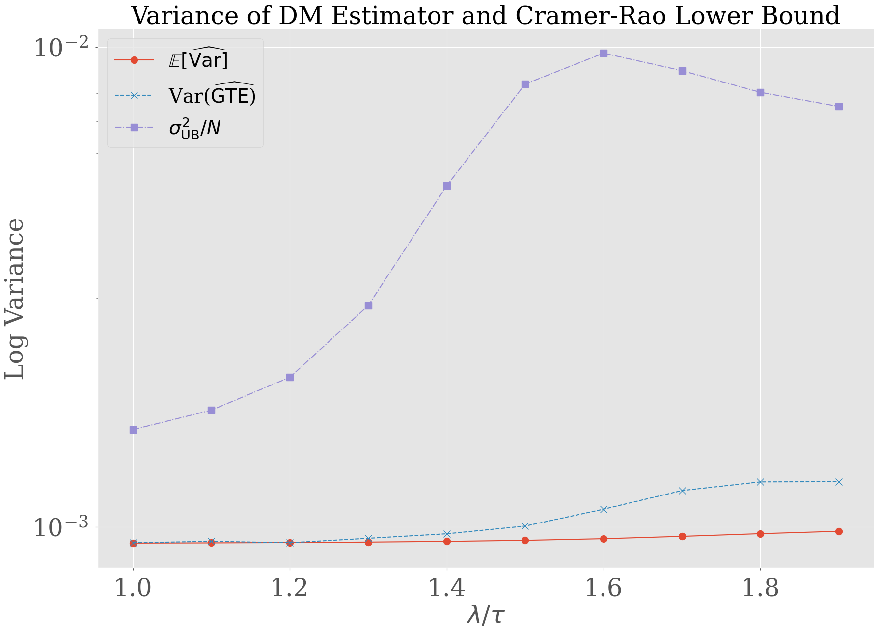
(b) $\lambda/\tau$ varying from $1.0$ to $2.0$, and other model parameters fixed as in Section C.1.

Figure 5: Variance comparison using data from Bernoulli randomized CR experiments, with $N=1000$ in all plots. The Cramér-Rao lower bound (cf. Theorem A.4) remains above the true variance of $\widehat{\mathsf{GTE}}$ and the variance estimator $\widehat{\mathrm{Var}}$ regardless of how we vary the model parameters. Error bars were omitted because they were so small that they were not visible on the plot.

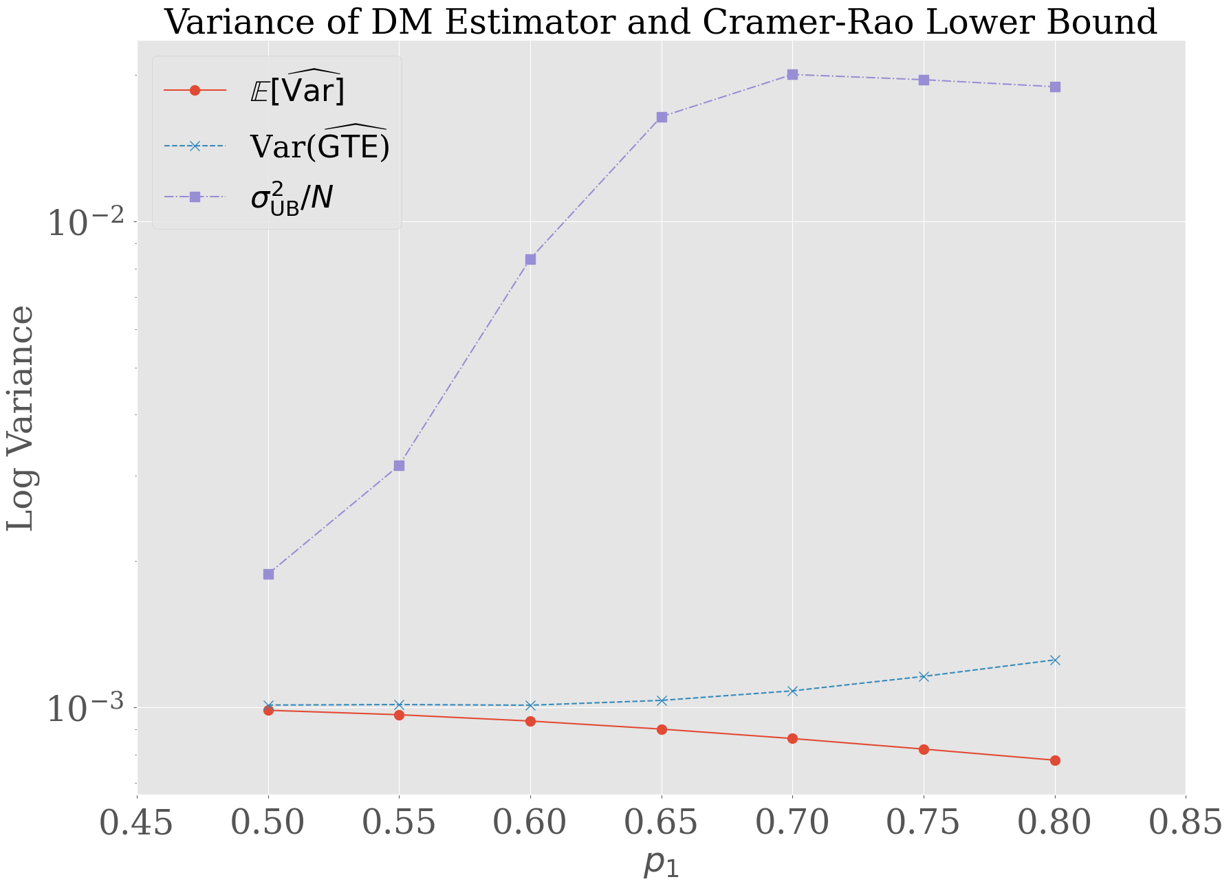
(a) $p_{1}$ varying from $0.5$ to $0.8$, and other model parameters fixed as in Section C.1.

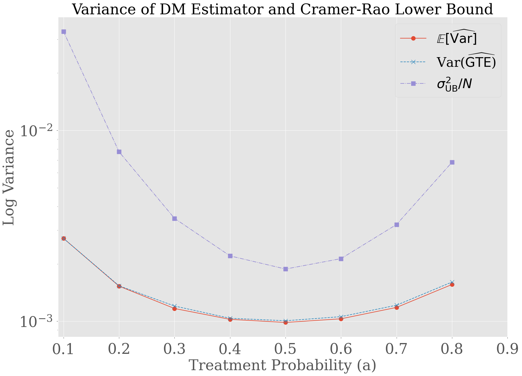
(b) $a$ varying from $0.1$ to $0.8$, and other model parameters fixed as in Section C.1.

Figure 6: Variance comparison using data from Bernoulli randomized CR experiments, with $N=1000$ in all plots. The Cramér-Rao lower bound (cf. Theorem A.4) remains above the true variance of $\widehat{\mathsf{GTE}}$ and the variance estimator $\widehat{\mathrm{Var}}$ regardless of how we vary the model parameters. Error bars are negligible and omitted from the plot.

C.3 Power comparisons under monotone treatments

In this section, we run $5\times 10^{4}$ Bernoulli randomized CR experiments with each of $K,\lambda/\tau,\boldsymbol{\mathrm{p}}_{1},a$ varying, and the other parameters fixed as described in Section C.1. We study the false negative probability of the decision rule (15) using the test statistic $\hat{T}_{N}$ (cf. (14)), and compare to the false negative probability obtained from the power calculation (25) for any test statistic that obeys (24). From Figures 7, 8, 9, and 10, we see that the decision rule using the test statistic $\hat{T}_{N}$ (cf. (14)) exhibits higher power than the same rule using any unbiased test statistic $\hat{U}_{N}$. In particular, the FNP of the test statistic $\hat{T}_{N}$ decays at a faster rate as $N$ increases in all cases.

Figure 7: Log false negative probability of decision rule (15) using the test statistic $\hat{T}_{N}$ (cf. (14)), compared to the log false negative probability of an unbiased test statistic (cf. (25)) using an unbiased estimator that obeys (24). Bernoulli randomized CR experiments with $N\in[10,1000]$, $K\in\{10,20,30,50\}$, and other model parameters fixed as in Section C.1. Error bars are negligible and omitted from the plot.

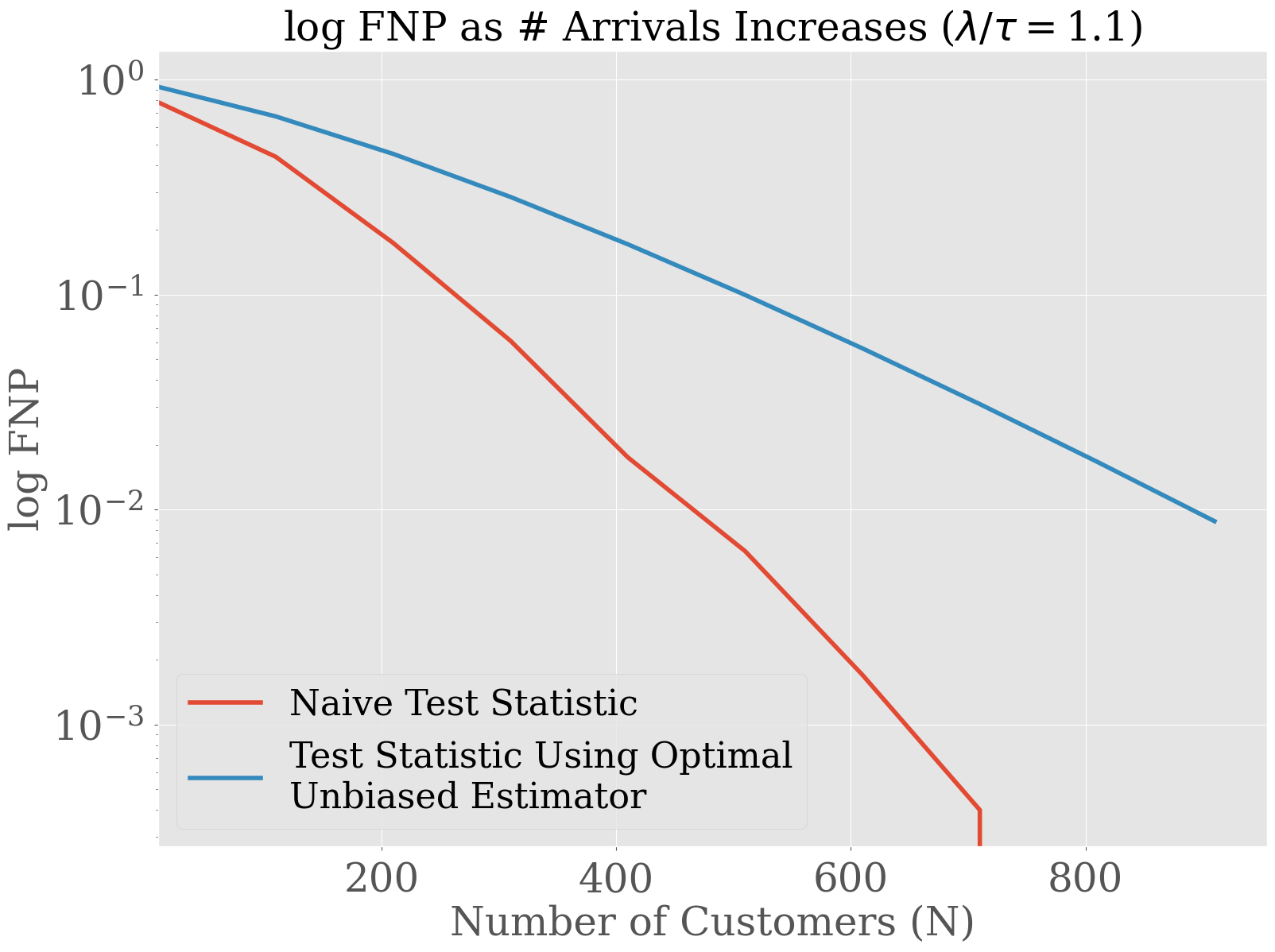
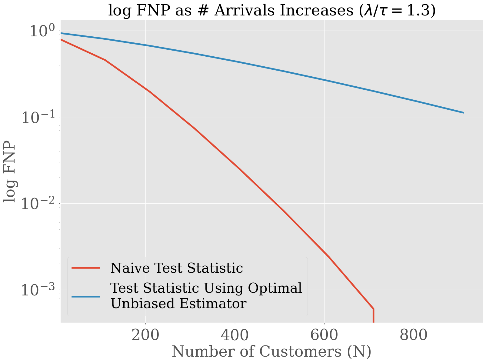
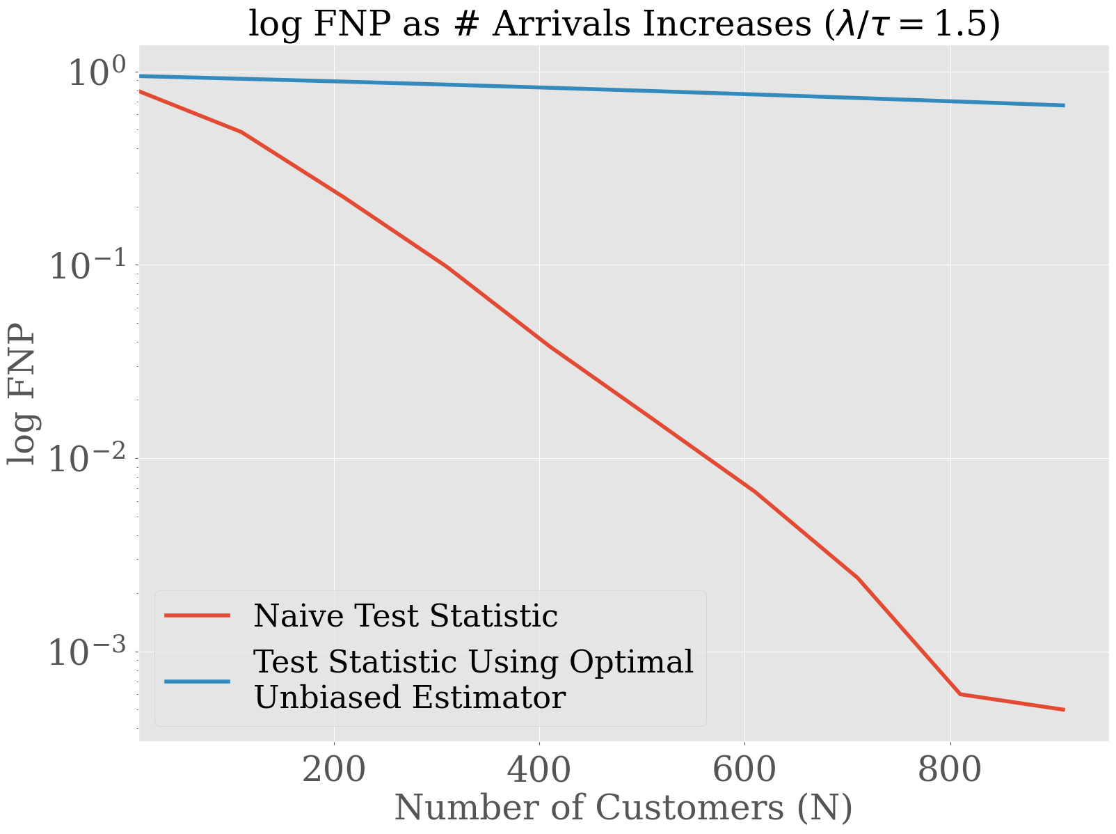
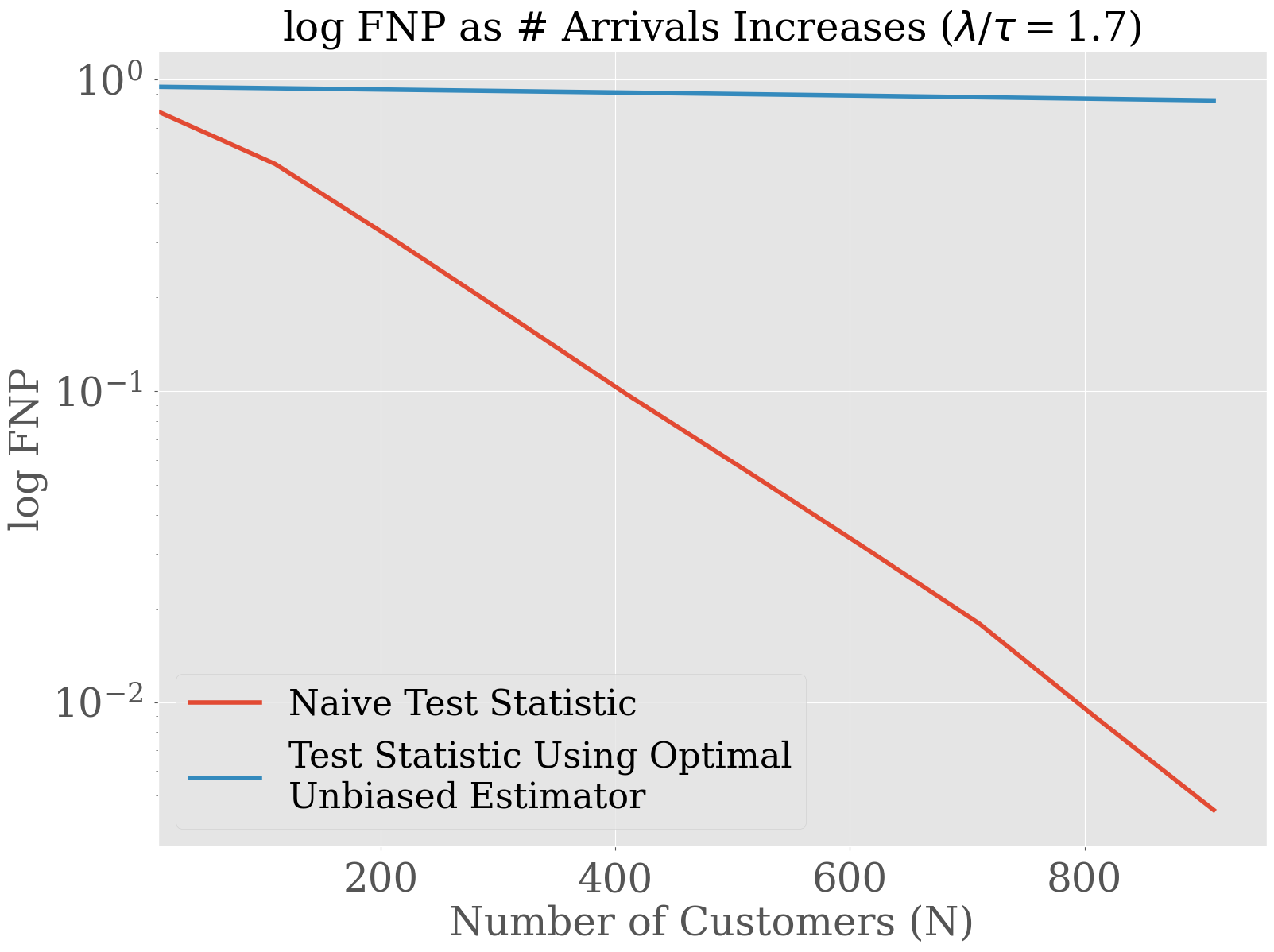
Figure 8: Log false negative probability of decision rule (15) using the test statistic $\hat{T}_{N}$ (cf. (14)), compared to the log false negative probability of an unbiased test statistic (cf. (25)) using an unbiased estimator that obeys (24). Bernoulli randomized CR experiments with $N\in[10,1000]$, $\lambda/\tau\in\{1.1,1.3,1.5,1.7\}$, and other model parameters fixed as in Section C.1. Error bars are negligible and omitted from the plot.

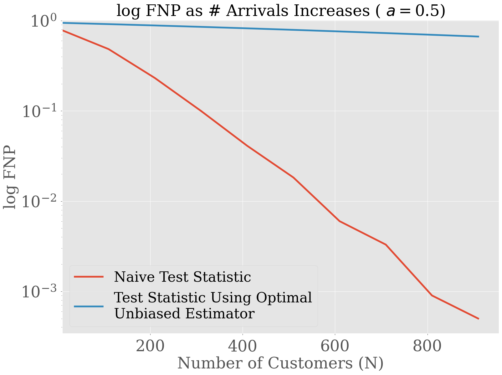
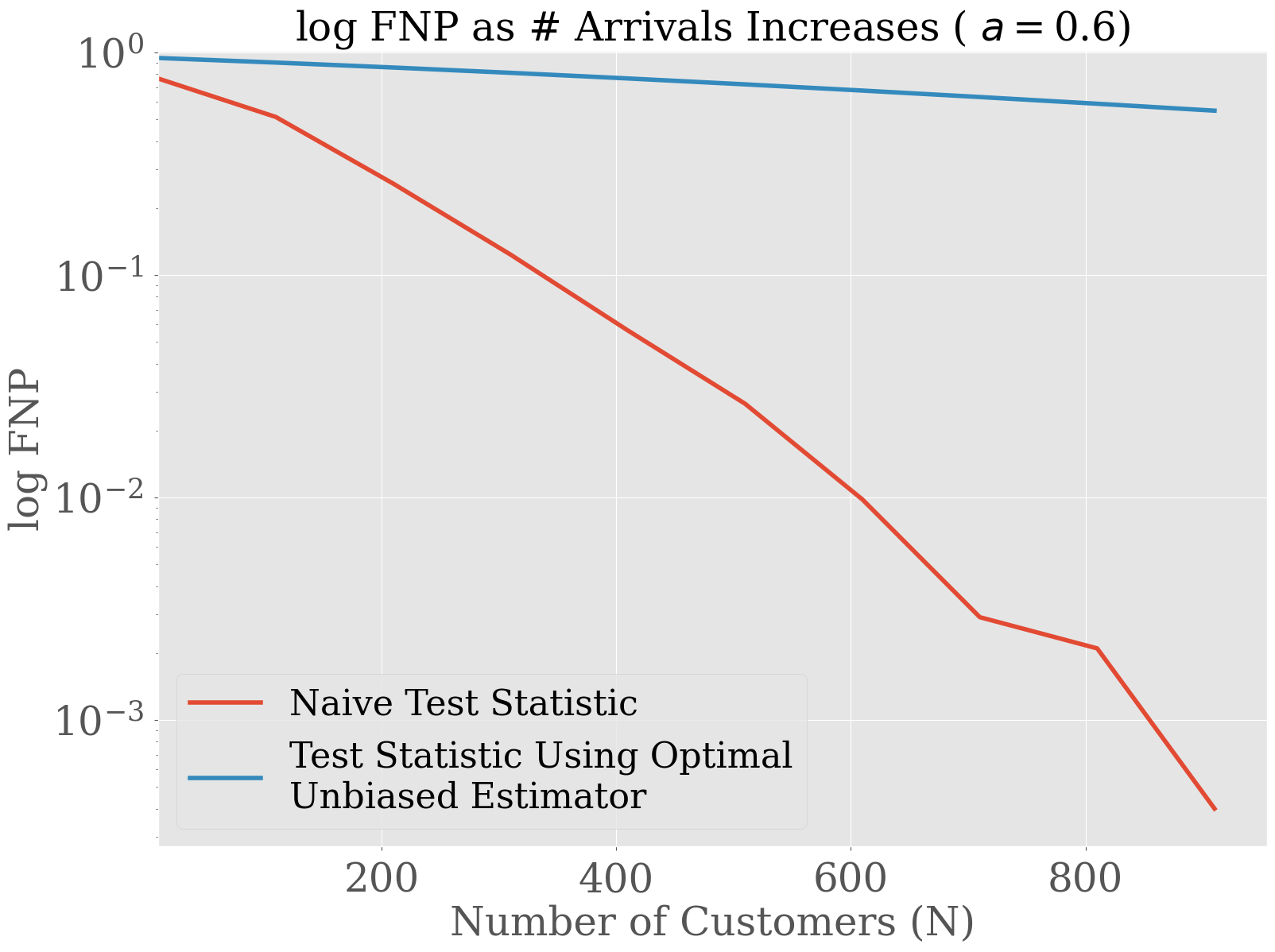
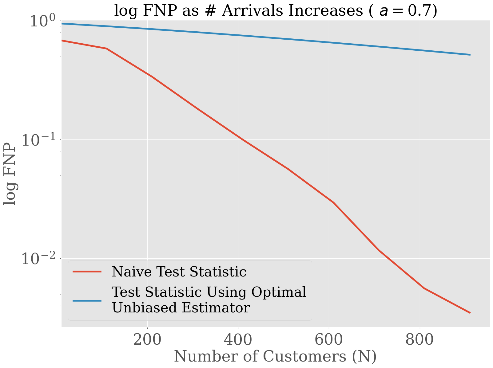
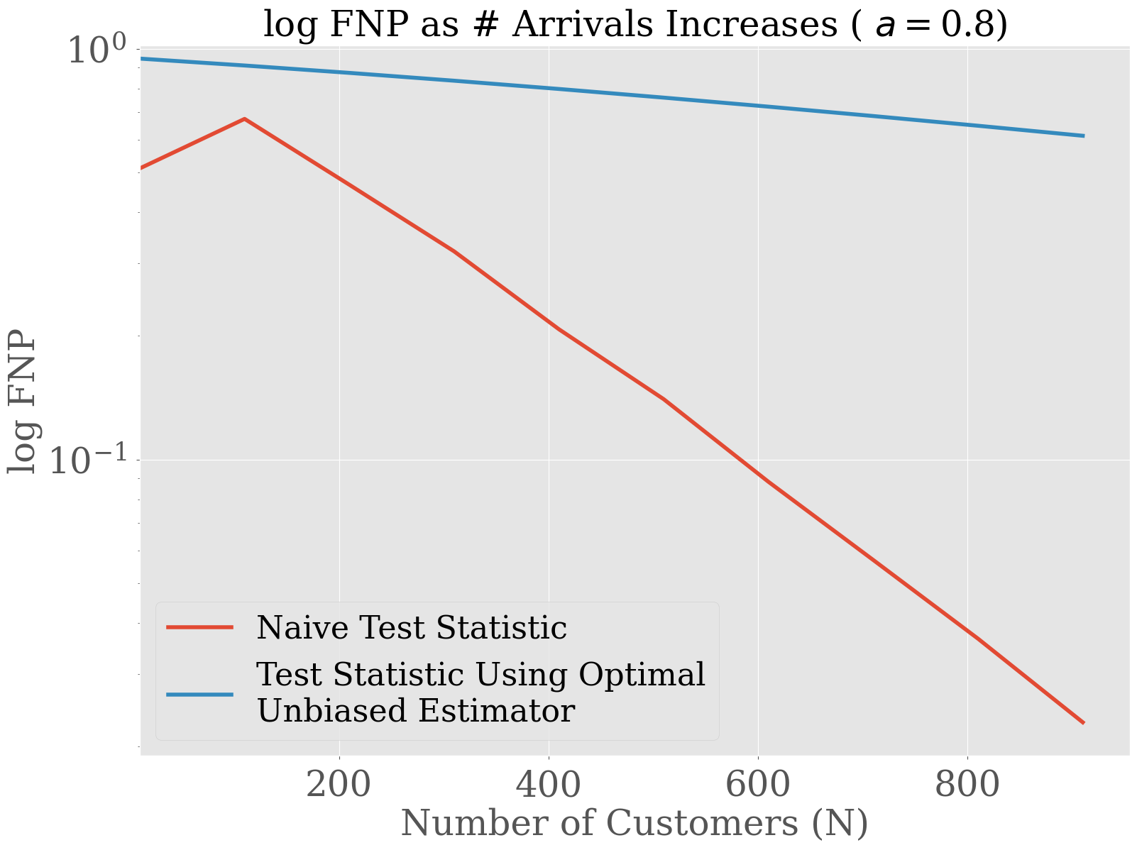
Figure 9: Log false negative probability of decision rule (15) using the test statistic $\hat{T}_{N}$ (cf. (14)), compared to the log false negative probability of an unbiased test statistic (cf. (25)) using an unbiased estimator that obeys (24). Bernoulli randomized CR experiments with $N\in[10,1000]$, $a\in\{0.5,0.6,0.7,0.8\}$, and other model parameters fixed as in Section C.1. Error bars are negligible and omitted from the plot.

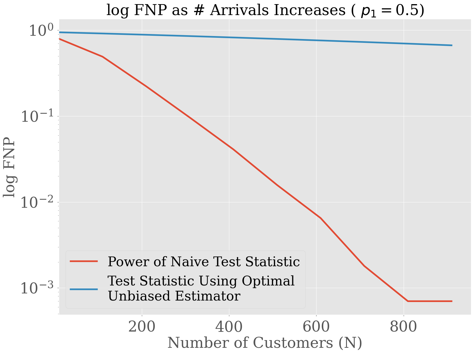
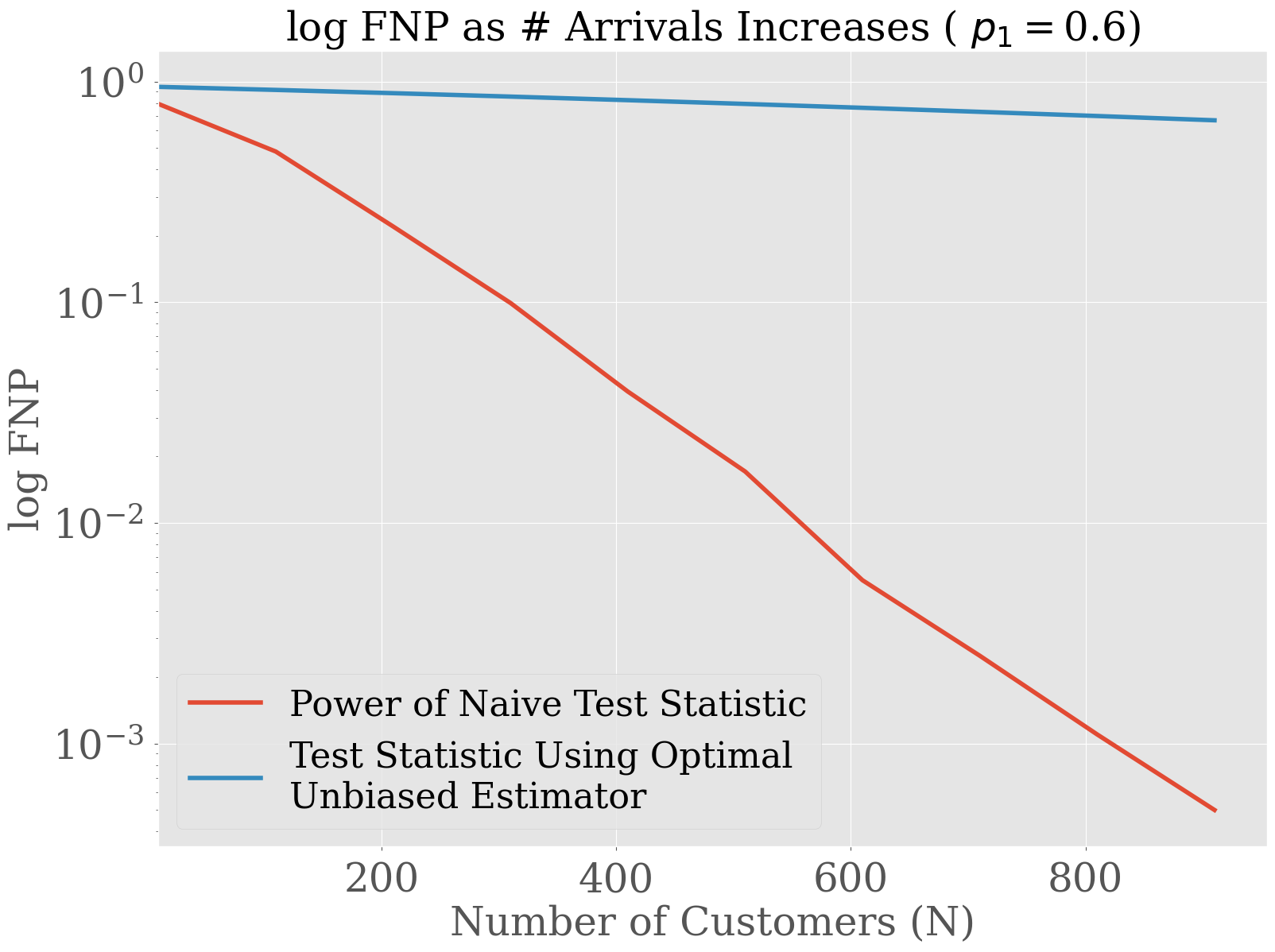
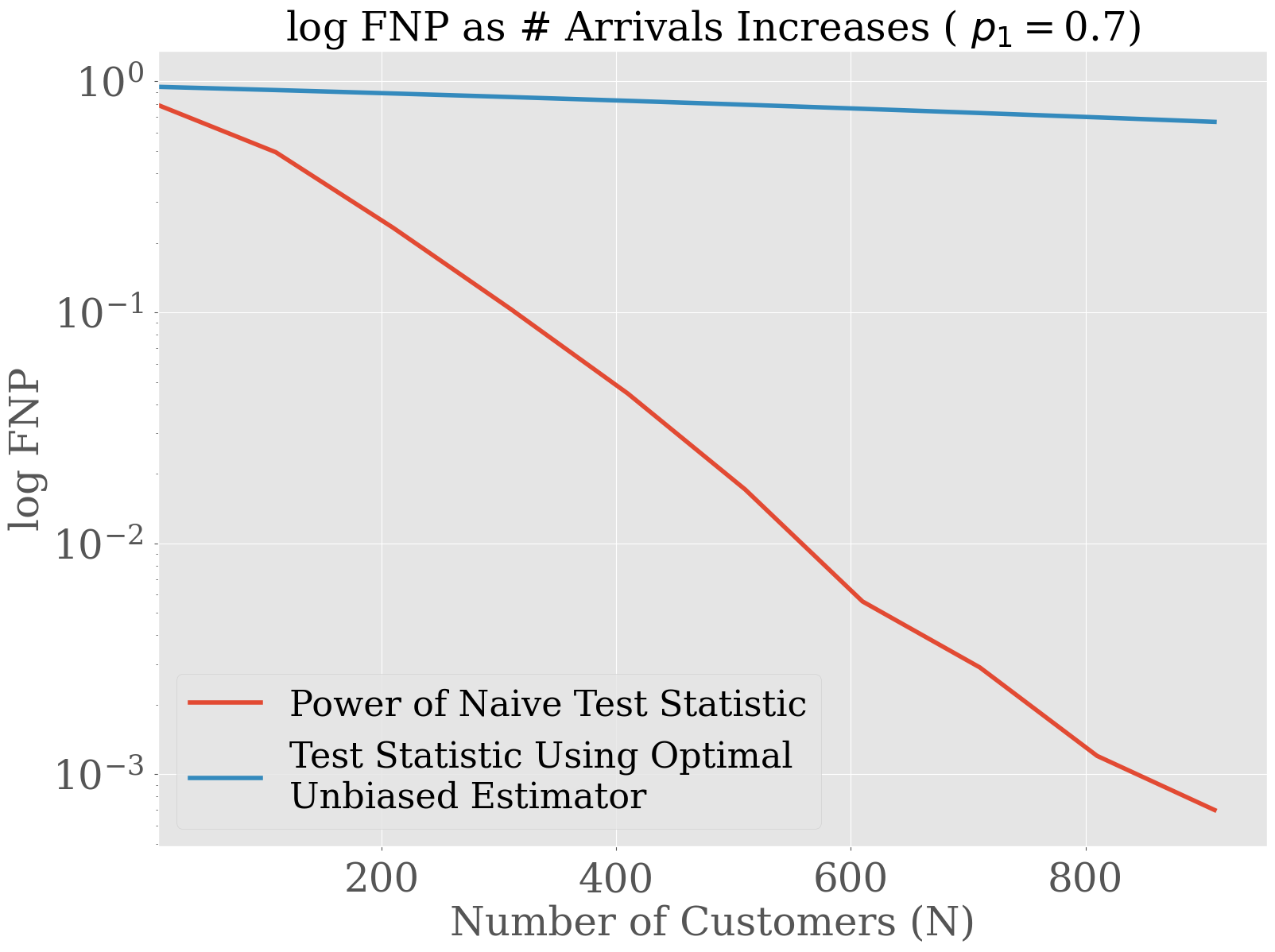
Figure 10: Log false negative probability of decision rule (15) using the test statistic $\hat{T}_{N}$ (cf. (14)), compared to the log false negative probability of an unbiased test statistic (cf. (25)) using an unbiased estimator that obeys (24). Bernoulli randomized CR experiments with $N\in[10,1000]$, $p_{1}\in\{0.5,0.6,0.7,0.8\}$, and other model parameters fixed as in Section C.1. Error bars are negligible and omitted from the plot.

References

- [1] P. M. Aronow and C. Samii. Estimating average causal effects under general interference, with application to a social network experiment. Annals of Applied Statistics, pages 1912–1947, 2017.
- [2] S. Athey, D. Eckles, and G. W. Imbens. Exact p-values for network interference. Journal of the American Statistical Association, 113(521):230–240, 2018.
- [3] E. M. Azevedo, A. Deng, J. L. Montiel Olea, J. Rao, and E. G. Weyl. A/B testing with fat tails. Journal of Political Economy, 128(12):4614–000, 2020.
- [4] P. Bajari, B. Burdick, G. W. Imbens, L. Masoero, J. McQueen, T. S. Richardson, and I. M. Rosen. Experimental design in marketplaces. Statistical Science, 38(3):458–476, 2023.
- [5] J. M. Bernardo and A. F. Smith. Bayesian theory, volume 405. John Wiley & Sons, 2009.
- [6] T. Blake and D. Coey. Why marketplace experimentation is harder than it seems: The role of test-control interference. In Proceedings of the fifteenth ACM conference on Economics and computation, pages 567–582, 2014.
- [7] J. Boutilier, J. O. Jonasson, H. Li, and E. Yoeli. Randomized controlled trials of service interventions: The impact of capacity constraints. arXiv preprint arXiv:2407.21322, 2024.
- [8] I. Bright, A. Delarue, and I. Lobel. Reducing marketplace interference bias via shadow prices. arXiv preprint arXiv:2205.02274, 2022.
- [9] W. Dhaouadi, R. Johari, and G. Y. Weintraub. Price experimentation and interference in online platforms. arXiv preprint arXiv:2310.17165, 2023.
- [10] D. Eckles, B. Karrer, and J. Ugander. Design and analysis of experiments in networks: Reducing bias from interference. Journal of Causal Inference, 5(1):20150021, 2017.
- [11] V. Farias, A. Li, T. Peng, and A. Zheng. Markovian interference in experiments. Advances in Neural Information Processing Systems, 35:535–549, 2022.
- [12] V. Farias, H. Li, T. Peng, X. Ren, H. Zhang, and A. Zheng. Correcting for interference in experiments: A case study at Douyin. In Proceedings of the 17th ACM Conference on Recommender Systems, pages 455–466, 2023.
- [13] E. M. Feit and R. Berman. Test & roll: Profit-maximizing A/B tests. Marketing Science, 38(6):1038–1058, 2019.
- [14] P. W. Glynn, R. Johari, and M. Rasouli. Adaptive experimental design with temporal interference: A maximum likelihood approach. Advances in Neural Information Processing Systems, 33:15054–15064, 2020.
- [15] M. A. Hernán and J. M. Robins. Estimating causal effects from epidemiological data. Journal of Epidemiology & Community Health, 60(7):578–586, 2006.
- [16] D. Holtz, R. Lobel, I. Liskovich, and S. Aral. Reducing interference bias in online marketplace pricing experiments. arXiv preprint arXiv:2004.12489, 2020.
- [17] S. R. Howard, A. Ramdas, J. McAuliffe, and J. Sekhon. Time-uniform, nonparametric, nonasymptotic confidence sequences. The Annals of Statistics, 49(2):1055–1080, 2021.
- [18] Y. Hu, S. Li, and S. Wager. Average direct and indirect causal effects under interference. Biometrika, 109(4):1165–1172, 2022.
- [19] Y. Hu and S. Wager. Switchback experiments under geometric mixing. arXiv preprint arXiv:2209.00197, 2022.
- [20] Y. Hu and S. Wager. Off-policy evaluation in partially observed markov decision processes under sequential ignorability. The Annals of Statistics, 51(4):1561–1585, 2023.
- [21] M. G. Hudgens and M. E. Halloran. Toward causal inference with interference. Journal of the American Statistical Association, 103(482):832–842, 2008.
- [22] G. W. Imbens and D. B. Rubin. Causal inference in statistics, social, and biomedical sciences. Cambridge university press, 2015.
- [23] R. Johari, P. Koomen, L. Pekelis, and D. Walsh. Peeking at A/B tests: Why it matters, and what to do about it. In Proceedings of the 23rd ACM SIGKDD International Conference on Knowledge Discovery and Data Mining, pages 1517–1525, 2017.
- [24] R. Johari, P. Koomen, L. Pekelis, and D. Walsh. Always valid inference: Continuous monitoring of A/B tests. Operations Research, 70(3):1806–1821, 2022.
- [25] R. Johari, H. Li, I. Liskovich, and G. Y. Weintraub. Experimental design in two-sided platforms: An analysis of bias. Management Science, 68(10):7069–7089, 2022.
- [26] G. L. Jones. On the Markov chain central limit theorem. Probability Surveys, 1(none):299–320, Jan. 2004. Publisher: Institute of Mathematical Statistics and Bernoulli Society.
- [27] N. Kallus and M. Uehara. Double reinforcement learning for efficient off-policy evaluation in markov decision processes. Journal of Machine Learning Research, 21(167):1–63, 2020.
- [28] J. Keilson and A. Kester. Monotone matrices and monotone markov processes. Stochastic Processes and their Applications, 5(3):231–241, 1977.
- [29] R. Kohavi and N. Chen. False positives in a/b tests. In Proceedings of the 30th ACM SIGKDD Conference on Knowledge Discovery and Data Mining, pages 5240–5250, 2024.
- [30] R. Kohavi, D. Tang, and Y. Xu. Trustworthy online controlled experiments: A practical guide to a/b testing. Cambridge University Press, 2020.
- [31] T. Lattimore and C. Szepesvári. Bandit algorithms. Cambridge University Press, 2020.
- [32] H. Li, G. Zhao, R. Johari, and G. Y. Weintraub. Interference, bias, and variance in two-sided marketplace experimentation: Guidance for platforms. In Proceedings of the ACM Web Conference 2022, pages 182–192, 2022.
- [33] S. Li, R. Johari, X. Kuang, and S. Wager. Experimenting under stochastic congestion. arXiv preprint arXiv:2302.12093, 2023.
- [34] P. Liao, P. Klasnja, and S. Murphy. Off-policy estimation of long-term average outcomes with applications to mobile health. Journal of the American Statistical Association, 116(533):382–391, 2021.
- [35] D. V. Lindley and M. R. Novick. The role of exchangeability in inference. The annals of statistics, pages 45–58, 1981.
- [36] R. Lucht. What is an A/A test? Full Guide with Examples — geteppo.com. https://www.geteppo.com/blog/what-is-an-aa-test. [Accessed 06-09-2024].
- [37] C. F. Manski. Identification of treatment response with social interactions. The Econometrics Journal, 16:S1–S23, 2013.
- [38] M. Mehrabi and S. Wager. Off-policy evaluation in markov decision processes under weak distributional overlap. arXiv preprint arXiv:2402.08201, 2024.
- [39] E. Munro, S. Wager, and K. Xu. Treatment effects in market equilibrium. arXiv preprint arXiv:2109.11647, 2021.
- [40] J. M. Robins and S. Greenland. Identifiability and exchangeability for direct and indirect effects. Epidemiology, 3(2):143–155, 1992.
- [41] L. Roemheld and J. Rao. Interference produces false-positive pricing experiments. arXiv preprint arXiv:2402.14538, 2024.
- [42] L. Rogers. The A/A Test: What You Need to Know — world.optimizely.com. https://world.optimizely.com/blogs/lindsey-rogers/dates/2024/4/the-aa-test-what-you-need-to-know/. [Accessed 04-09-2024].
- [43] P. R. Rosenbaum. Interference between units in randomized experiments. Journal of the american statistical association, 102(477):191–200, 2007.
- [44] B. A. Rosner. Fundamentals of biostatistics, volume 8. Cengage, 2016.
- [45] O. Saarela, D. A. Stephens, and E. E. Moodie. The role of exchangeability in causal inference. Statistical Science, 38(3):369–385, 2023.
- [46] S. Schmit, V. Shah, and R. Johari. Optimal testing in the experiment-rich regime. In The 22nd International Conference on Artificial Intelligence and Statistics, pages 626–633. PMLR, 2019.
- [47] J. Ugander, B. Karrer, L. Backstrom, and J. Kleinberg. Graph cluster randomization: Network exposure to multiple universes. In Proceedings of the 19th ACM SIGKDD international conference on Knowledge discovery and data mining, pages 329–337, 2013.
- [48] T. VanHaren. How to conduct an A/A test (and interpret the results!) — statsig.com. https://www.statsig.com/blog/how-to-aa-test#:~:text=A%2FA%20testing%20is%20useful,running%20more%20effective%20experiment%20reviews. [Accessed 06-09-2024].
- [49] S. Wager. Causal Inference: A Statistical Learning Approach. 2024.
- [50] S. Wager and K. Xu. Experimenting in equilibrium. Management Science, 67(11):6694–6715, 2021.