Rodimus*: Breaking the Accuracy-Efficiency Trade-Off with Efficient Attentions

Abstract

Recent advancements in Transformer-based large language models (LLMs) have set new standards in natural language processing. However, the classical softmax attention incurs significant computational costs, leading to a ${\mathcal{O}}(T)$ complexity for per-token generation, where $T$ represents the context length. This work explores reducing LLMs’ complexity while maintaining performance by introducing Rodimus and its enhanced version, Rodimus$+$. Rodimus employs an innovative data-dependent tempered selection (DDTS) mechanism within a linear attention-based, purely recurrent framework, achieving significant accuracy while drastically reducing the memory usage typically associated with recurrent models. This method exemplifies semantic compression by maintaining essential input information with fixed-size hidden states. Building on this, Rodimus$+$ combines Rodimus with the innovative Sliding Window Shared-Key Attention (SW-SKA) in a hybrid approach, effectively leveraging the complementary semantic, token, and head compression techniques. Our experiments demonstrate that Rodimus$+$-1.6B, trained on 1 trillion tokens, achieves superior downstream performance against models trained on more tokens, including Qwen2-1.5B and RWKV6-1.6B, underscoring its potential to redefine the accuracy-efficiency balance in LLMs. Model code and pre-trained checkpoints will be available soon.

1 Introduction

Recent advancements have positioned Transformer-based large language models (LLMs) at the forefront of natural language processing, establishing them as state-of-the-art. Their strong capabilities stem from the softmax attention mechanism, which selectively focuses on relevant tokens stored in the key-value (KV) cache when predicting the next token. By maintaining a historical record of tokens, the KV cache allows all pertinent data to remain accessible during inference. However, the demand to store this extensive historical information incurs notable computational costs, leading to ${\mathcal{O}}(T)$ complexity for per-token generation, where $T$ represents the length of the context preceding the generated token. Indeed, a 7B Llama [1]), without inference optimization, takes over a minute to generate 2K-length sequences on an A10-24G [2].

This has sparked research into next-generation foundation models aimed at efficient alternatives to attention. Among them, three main categories stand out that aim to compress the KV cache in the original softmax attention from distinct perspectives: semantic, token, and head compression.

Semantic Compression: The first category, also known as linear attention [3], or linear state space models (SSMs) [4, 5], substitutes the exponential kernel in softmax attention with a simplified inner product of (transformed) query and key vectors. This approach results in a recurrently updated hidden state of fixed size that retains historical semantic information like linear RNNs [6, 7], successfully reducing the per-token generation complexity from ${\mathcal{O}}(T)$ to ${\mathcal{O}}(1)$. However, compressing the softmax attention—characterized by its unlimited capacity—into linear attention with fixed capacity inevitably leads to some information loss. To address this, current methods strive to (i) increase the recurrent state size to enhance memory capacity [8] and (ii) utilize the fixed-sized states more effectively [9]. Despite these advancements, there remains a trade-off between complexity and performance (refer to Figure 1). Blindly expanding the hidden states compromises time and space efficiency, while incorporating data-dependent decay or gating mechanisms to filter out irrelevant past information may hinder parallel training efficiency, as noted in [10].

Token Compression: This second category introduces sparsity into the attention mask, allowing it to follow predefined patterns and focus on strategically chosen tokens, such as those at the beginning of a sequence or close to the answer [11, 12]. Consequently, this method can also achieve the ${\mathcal{O}}(1)$ complexity for per-token generation. However, the elimination of masked tokens can lead to a complete loss of information and potentially degrade the overall performance.

Head Compression: The third category reshapes attention by modifying the design of attention heads. This involves grouping heads and sharing keys and values within each group, as seen in multi-query attention (MQA) [13] and grouped-query attention (GQA) [14]. While these methods reduce the cache size by a constant factor, they are inherently lossy compared to multi-head attention (MHA) [15] as the same values are used within each group.

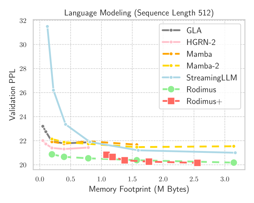
(a) LM Task on the WikiText-103 Dataset.

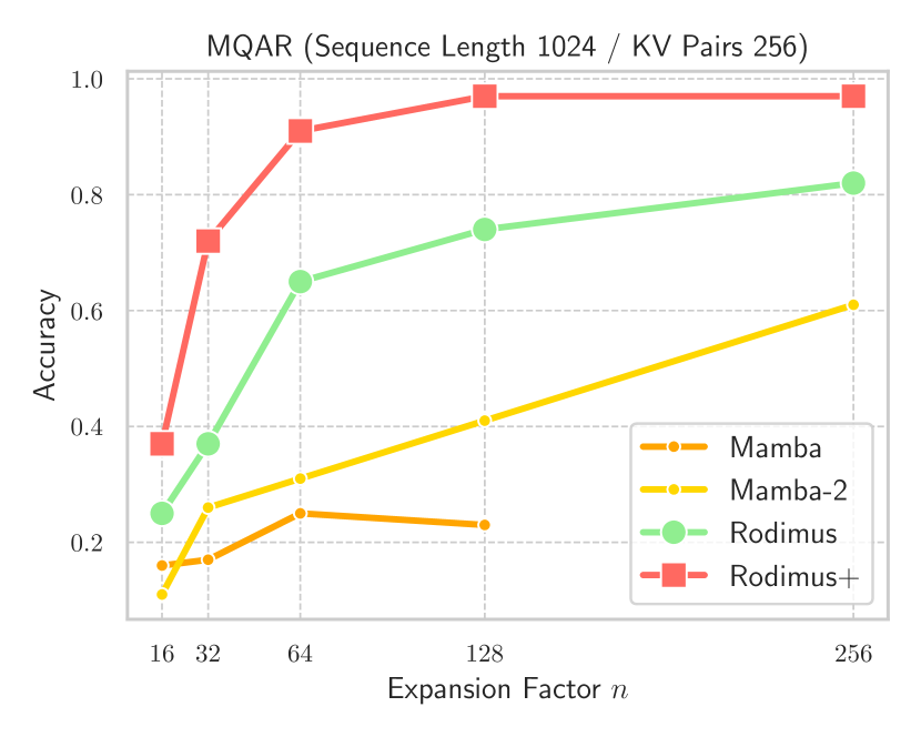
(b) Multi-Query Associative Recall (MQAR) Task.

Figure 1: Memory Footprint vs. Performance: (a) This experiment is conducted on the WikiText-103 dataset (see Section 4.1), and focuses on the recorded best perplexity (PPL). The memory footprint is adjusted by modifying the expansion factor. (b) The model’s recall capability is assessed using the MQAR Task, as described in [16]. Among all models evaluated, Rodimus* achieves the optimal balance between space complexity and performance.

Ultimately, none of these methods can fully supplant the original softmax attention, prompting an essential question: Is it feasible to reduce the complexity of LLMs while preserving performance? Our research affirms this possibility, showing that a linear attention model enhanced with a well-designed data-dependent tempered selection (DDTS) mechanism—an improvement within the first category—and its hybridization with our proposed sliding window shared-key attention (SW-SKA), which integrates all three types of attention compressions, offers viable solutions. We designate the former model as Rodimus and the latter as Rodimus$+$. Remarkably, Rodimus maintains a much smaller hidden state size than most current SOTA recurrent models (e.g., half of the size in Mamba2 [5]), but outperforms softmax attention-based Transformers. Moreover, Rodimus$+$-1.6B (trained on 1 trillion tokens) achieves an average performance that is 0.31% higher than Qwen2-1.5B (trained on 7 trillion tokens) and 2.3% higher than RWKV6-1.6B (trained on 1.4 trillion tokens) in downstream task evaluations. Our contributions can be summarized as follows:

• We introduce a linear attention-based, purely recurrent model, Rodimus, effectively overcoming the accuracy-efficiency trade-off found in existing recurrent models. By incorporating the innovative DDTS, Rodimus can autonomously filter out irrelevant information during semantic compression, resulting in improved validation perplexity (PPL) with much smaller memory footprints compared to other SOTA methods, as illustrated by the green curves in Figure 1.

• We present a hybrid model, Rodimus$+$, which combines Rodimus with the innovative SW-SKA. While the recurrent hidden state in Rodimus offers a comprehensive semantic view of the historical context, the sliding window attention highlights the nearby tokens that are most influential in predicting the next token, and SKA further compresses cache size in a lossless manner. As shown by the red curves in Figure 1, Rodimus$+$ continues to extend the accuracy-efficiency frontier of existing methods, achieving superior performance with reduced complexity.

• We validate the effectiveness of Rodimus* (encompassing both Rodimus and Rodimus$+$) through thorough experimentation. In downstream evaluations with model sizes from 130M to 1.3B, Rodimus* demonstrates enhanced language modeling performance relative to current SOTA models of similar sizes. Furthermore, Rodimus* achieves a performance improvement of up to 7.21% over Mamba2, and outperforms even softmax attention-based Pythia on NeedleBench—a suite of recall-intensive tasks where recurrent models typically underperform [17].

2 Preliminaries

In this section, we provide a brief introduction to softmax attention in [15] and derive its recurrent form. We will then derive the aforementioned three attention compression methods, including linear attention for semantic compression, sparse attention for token compression, and sharing-based attention for head compression. The first two methods simplify attention by reducing context length, while the last one makes modifications along the dimension of attention heads.

Softmax Attenion and its Recurrent Form: Suppose that ${\bm{X}}=\{{\bm{x}}_{1},\dots,{\bm{x}}_{T}\}\in\mathbb{R}^{T\times d}$ denotes the input sequence with length $T$ and dimension $d$. Standard autoregressive Transformers [15] utilize a softmax attention mechanism to generate the output ${\bm{O}}\in\mathbb{R}^{T\times d}$, that is,

$${\bm{Q}},{\bm{K}},{\bm{V}}={\bm{X}}{\bm{W}}_{Q},{\bm{X}}{\bm{W}}_{K},{\bm{X}}{\bm{W}}_{V},\quad{\bm{O}}=\mathrm{softmax}\left(({\bm{Q}}{\bm{K}}^{\top})\odot{\bm{M}}\right){\bm{V}},$$ (1)

where ${\bm{W}}_{Q}\in\mathbb{R}^{d\times n},{\bm{W}}_{K}\in\mathbb{R}^{d\times n},{\bm{W}}_{V}\in\mathbb{R}^{d\times m}$ are learnable weight matrix associated with the queries ${\bm{Q}}$, the keys ${\bm{K}}$, and values ${\bm{V}}$, respectively. The matrix ${\bm{M}}\in\{-\infty,1\}\in\mathbb{R}^{T\times T}$ denotes the upper-triangular attention mask, ensuring that the model does not attend to future tokens. Multi-Head Attention (MHA) further splits the dimensionality $d$ into $h$ heads, computing attention for each head in $\mathbb{R}^{d_{h}}$ individually with distinct weights. This approach enhances the model’s capacity to capture diverse sequential information while reducing the computational costs for matrix operations.

The above parallel form allows for the computation of ${\bm{O}}=\{{\bm{o}}_{1},\dots,{\bm{o}}_{T}\}$ in parallel given the full input ${\bm{X}}$, facilitating efficient training. In contrast, during inference, Transformers rely on the following recurrent formulation [3]:

$${\bm{q}}_{t},{\bm{k}}_{t},{\bm{v}}_{t}={\bm{x}}_{t}{\bm{W}}_{Q},{\bm{x}}_{t}{\bm{W}}_{K},{\bm{x}}_{t}{\bm{W}}_{V},\quad{\bm{o}}_{t}=\frac{\sum_{i=1}^{t}\exp({\bm{q}}_{t}{\bm{k}}_{i}^{\top}){\bm{v}}_{i}}{\sum_{i=1}^{t}\exp({\bm{q}}_{t}{\bm{k}}_{i}^{\top})}.$$ (2)

Here, the query ${\bm{q}}_{t}\in\mathbb{R}^{1\times n}$, key ${\bm{k}}_{t}\in\mathbb{R}^{1\times n}$, and value ${\bm{v}}_{t}\in\mathbb{R}^{1\times m}$ vectors are computed based on the representation of current token ${\bm{x}}_{t}\in\mathbb{R}^{1\times d}$. Attention is subsequently performed over the evolving collection of keys $\{{\bm{k}}_{1},\dots,{\bm{k}}_{t}\}$ and values $\{{\bm{v}}_{1},\dots,{\bm{v}}_{t}\}$ (i.e., the KV cache). Thus, the time and space complexity for generating the next token at time stamp $t$ is ${\mathcal{O}}(t)$.

Linear Attention for Semantic Compression: To optimize efficiency, linear attention mechanisms replace the exponential kernel $\exp({\bm{q}}_{t}{\bm{k}}_{i}^{\top})$ in Eq. (2) by a kernel $k({\bm{q}}_{t},{\bm{k}}_{i})$ paired with an associated feature map $\phi$, i.e., $k({\bm{q}}_{t},{\bm{k}}_{i})=\phi({\bm{q}}_{t})\phi({\bm{k}}_{i})^{\top}$. As a result, the calculation of ${\bm{o}}_{t}$ can be simplified as:

$${\bm{o}}_{t}=\frac{\sum_{i=1}^{t}\phi({\bm{q}}_{t})\phi({\bm{k}}_{i})^{\top}{\bm{v}}_{i}}{\sum_{i=1}^{t}\phi({\bm{q}}_{t})\phi({\bm{k}}_{i})^{\top}}=\frac{\phi({\bm{q}}_{t})\sum_{i=1}^{t}\phi({\bm{k}}_{i})^{\top}{\bm{v}}_{i}}{\phi({\bm{q}}_{t})\sum_{i=1}^{t}\phi({\bm{k}}_{i})^{\top}}.$$ (3)

Letting ${\bm{S}}_{t}=\sum_{i=1}^{t}\phi({\bm{k}}_{i})^{\top}{\bm{v}}_{i}\in\mathbb{R}^{n\times m}$ and ${\bm{z}}_{t}=\sum_{i=1}^{t}\phi({\bm{k}}_{i})^{\top}\in\mathbb{R}^{n\times 1}$ be the KV state and the K state respectively, we can rewrite the previous equation as a linear state-space model (SSM) or RNN:

$${\bm{S}}_{t}={\bm{S}}_{t-1}+\phi({\bm{k}}_{t})^{\top}{\bm{v}}_{t},\quad{\bm{z}}_{t}={\bm{z}}_{t-1}+\phi({\bm{k}}_{t})^{\top},\quad{\bm{o}}_{t}=\frac{\phi({\bm{q}}_{t}){\bm{S}}_{t}}{\phi({\bm{q}}_{t}){\bm{z}}_{t}}.$$ (4)

We emphasize that ${\bm{S}}_{t}$ provides a semantic compression of the historical context up to $t$. The denominator $\phi({\bm{q}}_{t}){\bm{z}}_{t}\in\mathbb{R}$ may introduce numerical instabilities and hinder the optimization [18], prompting many recent studies to replace it with a normalization [18, 19]. Moreover, it is common to use the identity mapping for $\phi$ [19, 9], and so Eq. (4) amounts to

$${\bm{S}}_{t}={\bm{S}}_{t-1}+{\bm{k}}_{t}^{\top}{\bm{v}}_{t},\quad{\bm{o}}_{t}={\bm{q}}_{t}{\bm{S}}_{t}.$$ (5)

More generally, when framed within the context of linear SSMs [4, 5] or RNNs [20], these equations can be reformulated as:

$${\bm{S}}_{t}={\bm{A}}_{t}\odot{\bm{S}}_{t-1}+{\bm{B}}_{t}\odot{\bm{u}}_{t},\quad{\bm{o}}_{t}={\bm{C}}_{t}{\bm{S}}_{t},$$ (6)

where ${\bm{A}}_{t}=1$, ${\bm{B}}_{t}=1$, and ${\bm{C}}_{t}={\bm{q}}_{t}$ represent the state transition, input, and output matrix respectively, while ${\bm{u}}_{t}={\bm{k}}_{t}^{\top}{\bm{v}}_{t}$ signifies the input or control. In stark contrast to softmax attention, the per-token generation complexity at time stamp $t$ is ${\mathcal{O}}(1)$, enabling efficient inference. Meanwhile, linear attention can be expressed in a parallel form similar to Eq. (1), allowing for training parallelism.

However, this additive formulation of updating the hidden states ${\bm{S}}_{t}$ with new key-value pairs at each time step $t$ does not possess the capability to forget irrelevant information, which leads to the phenomenon known as attention dilution [21, 18]. To address this concern, recent works (i) increase the state size (either $n$ or $d_{h}$) to retain more information and (ii) incorporate decay factors or gating mechanisms that enable the state ${\bm{S}}_{t}$ to discard irrelevant past information. The first approach typically sacrifices efficiency for performance, whereas the second method focuses on designing ${\bm{A}}_{t}$ and ${\bm{B}}_{t}$ to manage memory retention and forgetting behaviors within the hidden states.

We summarize the functional forms of ${\bm{A}}_{t}$ and ${\bm{B}}_{t}$ used in the SOTA methods in Table 4. Three major trends can be gleaned from this table. Firstly, it is beneficial for ${\bm{A}}_{t}$ and ${\bm{B}}_{t}$ to be negatively correlated, as shown in Mamba [4], Mamba2 [5], and HGRN2 [8], allowing them to collaboratively regulate the deletion and addition of information in the hidden state ${\bm{S}}_{t}$. This contrasts with methods like RetNet [19], gRetNet [22], and GLA [9], which use ${\bm{A}}_{t}$ as a decay factor while keeping ${\bm{B}}_{t}$ constant at 1. Secondly, allowing ${\bm{A}}_{t}$ and ${\bm{B}}_{t}$ to be functions of the input ${\bm{u}}_{t}$ enables dynamic adjustments over time in a data-dependent manner. This approach has been validated by the superior performance of GLA [9], gRetNet [22] compared to RetNet[19]. Lastly, designs for gating mechanisms must be compatible with GPU acceleration, ensuring that the recurrent expression (6) aligns with a parallel format, similarly to (1).

In Section 3.1, we further analyze these functional forms in relation to their equivalence with linear attention and propose a novel data-dependent tempered selection (DDTS) mechanism. This mechanism is capable of succinctly compressing historical information within a recurrent hidden state of fixed capacity, all while facilitating parallel training.

Sparse Attention for Token Compression: This group of methods aim to sparsify the attention mask ${\bm{M}}$ in Eq. (1). The goal is to compute only the $({\bm{q}}_{t},{\bm{k}}_{i})$ pairs associated with nonzero elements of ${\bm{M}}_{ti}$. Various types of attention masks have been proposed in the literature, including window attention [23], dilated attention [24], and bridge attention [25], among others. Research shows that the softmax attention maps in vanilla Transformer models often exhibit a localized behavior [18, 21, 11]. Thus, we exploit a sliding window (SW) attention to enhance the local context understanding in Rodimus$+$.

Sharing-based Attention for Head Compression: In the original MHA, each head has distinct linear transformations ${\bm{W}}_{Q},{\bm{W}}_{K},{\bm{W}}_{V}$ for the input ${\bm{X}}$, allowing for diverse representations and attention maps across heads. Sharing-based attention seek to compress the MHA by allowing key and value heads to be shared among multi-query heads. Specifically, in MQA [13], all heads use a single set of key and value weights, which reduces parameters and memory usage but risks diminishing the attention mechanism’s expressiveness. As a better alternative, GQA assigns one key and value head for each group of query heads [14]. However, it still limits the expressiveness of the original MHA by overly constraining learned relationships. As a remedy, we propose the Shared-Key Attention (SKA) in Section 3.2.1, which compresses the MHA while preserving its expressiveness.

3 Methodology

In this section, we introduce two models: Rodimus and Rodimus$+$, whose architecture is depicted in Figure 2. Rodimus is a purely recurrent model that iteratively compresses historical context into a fixed-size hidden state (i.e., semantic compression) and further exploits this state for the next token prediction. With the equipment of the newly proposed DDTS mechanism, Rodimus effectively filters out irrelevant information, thereby enhancing performance while reducing the size of the hidden state. On the other hand, Rodimus$+$ builds upon Rodimus by integrating the proposed SW-SKA technique. This enhancement improves performance without sacrificing efficiency, allowing for a seamless combination of semantic, token, and head compression methods.

Figure 2: Overview of the Proposed Models. The Rodimus* Model serves as a template for both Rodimus and Rodimus$+$. When modules within the gray dashed box are included, it becomes the Rodimus$+$ Model; otherwise, it is the Rodimus Model. The architecture comprises $L$ layers of stacked Rodimus* Blocks along with essential modules for language modeling (e.g., Embedding, RMSNorm, LM Head). Rodimus Flow (11) denotes our proposed recurrent computation method. The purple arrows depict information flow between layers (ignoring RMSNorm). In the Rodimus$+$ Model, the Rodimus block compresses the Token Embedding into a global semantic embedding, enhancing SW-SKA’s ability to perceive long contexts.

3.1 Rodimus: Overcoming Performance Bottleneck in Semantic Compression

3.1.1 Analysis of Existing Linear Attention Models

As can be observed from Table 4, the state transition equation in all existing linear attention models can be expressed recurrently as:

$${\bm{S}}_{t}=({\bm{\alpha}}_{t}^{\top}{\bm{\beta}}_{t})\odot{\bm{S}}_{t-1}+(\hat{\bm{\alpha}}_{t}^{\top}\hat{\bm{\beta}}_{t})\odot({\bm{k}}_{t}^{\top}{\bm{v}}_{t})=({\bm{\alpha}}_{t}^{\top}{\bm{\beta}}_{t})\odot{\bm{S}}_{t-1}+(\hat{\bm{\alpha}}_{t}\odot{\bm{k}}_{t})^{\top}(\hat{\bm{\beta}}_{t}\odot{\bm{v}}_{t}),$$ (7)

where ${\bm{\alpha}}_{t}\in\mathbb{R}^{1\times n}$ and ${\bm{\beta}}_{t}\in\mathbb{R}^{1\times m}$ denotes the gating mechanism along the dimension of $n$ and $m$ respectively, and $\hat{\bm{\alpha}}_{t}$ and $\hat{\bm{\beta}}_{t}$ are negatively correlated with ${\bm{\alpha}}_{t}$ and ${\bm{\beta}}_{t}$, allowing them to select between the current input ${\bm{u}}_{t}={\bm{k}}_{t}^{\top}{\bm{v}}_{t}$ and the previous state ${\bm{S}}_{t-1}$. Substituting Eq. (7) into Eq. (6) and unfolding the recurrent relation yields:

$${\bm{o}}_{t}=\sum_{i=1}^{t}\bigg{[}{\bm{q}}_{t}\big{(}\prod_{j=i+1}^{t}{\bm{\alpha}}_{j}\odot\hat{\bm{\alpha}}_{i}\odot{\bm{k}}_{i}\big{)}^{\top}\bigg{]}\big{(}\prod_{j=i+1}^{t}{\bm{\beta}}_{j}\odot\hat{\bm{\beta}}_{i}\odot{\bm{v}}_{i}\big{)}.$$ (8)

Here, $\prod_{j=i+1}^{t}{\bm{\alpha}}_{j}$ captures the relative positional information between time stamp $t$ and $i$, specifically between the query ${\bm{q}}_{t}$ and the key ${\bm{k}}_{i}$. Indeed, this component acts as a more flexible version of relative positional embeddings for softmax attention (e.g., xPos [26] and ALiBi [27]). In addition, the elements within the vector ${\bm{\alpha}}_{j}$ vary from one another, enabling the capture of high- and low-frequency information akin to sinusoidal positional encoding [15] and RoPE [28]. Notably, $\prod_{j=i+1}^{t}{\bm{\alpha}}_{j}$ also incorporates absolute positional information since it is also a function of the absolute positions $j=i+1,\dots,t$. Consequently, linear attention models expressed in the form of Eq. (7) capture first-order dependencies within sequences in a position-aware manner. In contrast, the original softmax attention (1) captures only second-order dependencies in a position-agnostic framework, necessitating the addition of positional embeddings [29].

On the other hand, $\prod_{j=i+1}^{t}{\bm{\beta}}_{j}$ also regulates the relative positional information between the time stamp $t$ and $i$, but between the query ${\bm{q}}_{t}$ and the value ${\bm{v}}_{i}$. This aspect has not been witnessed in softmax attention. Moreover, earlier studies [9] and our ablation study (see Table 13) indicate that incorporating $\prod_{j=i+1}^{t}{\bm{\beta}}_{j}$ cannot result in improvements compared to setting ${\bm{\beta}}_{j}=\mathbf{1}_{m}$, probably because such positional information has already been described by $\prod_{j=i+1}^{t}{\bm{\alpha}}_{j}$. Moreover, including ${\bm{\beta}}_{j}$ can impede training efficiency, as the dimensionality of ${\bm{\beta}}_{t}\in\mathbb{R}^{1\times m}$ is significantly larger than that of ${\bm{\alpha}}_{t}\in\mathbb{R}^{1\times n}$. This discrepancy can lead to redundant I/O operations when ${\bm{\beta}}_{j}$ are frequently transferred between high bandwidth memory (HBM) and on-chip SRAM during chunkwise parallelism (cf. Appendix C.3).

As a consequence, our focus is on optimizing the design of ${\bm{\alpha}}_{t}$ while setting ${\bm{\beta}}_{t}=\mathbf{1}_{m}$ for all $t$. We retain $\hat{\bm{\beta}}_{t}$ to allow for flexible selection among the various elements in the value vector ${\bm{v}}_{t}$.

3.1.2 Design of $\alpha_{t}$, $\hat{\alpha}_{t}$ and $\hat{\beta}_{t}$

We propose the following formulations for ${\bm{\alpha}}_{t}$ and $\hat{\bm{\alpha}}_{t}$:

$${\bm{\alpha}}_{t}=\exp(-{\bm{g}}_{t}\odot{\bm{\tau}}_{t}),\quad\hat{\bm{\alpha}}_{t}={\bm{g}}_{t}^{{\bm{\tau}}_{t}},$$ (9)

where ${\bm{g}}_{t}=\zeta({\bm{x}}_{t}{\bm{W}}_{g}+{\bm{b}}_{g})$ and ${\bm{\tau}}_{t}=\sigma({\bm{x}}_{t}{\bm{W}}_{\tau}+{\bm{b}}_{\tau})$. In this design, ${\bm{g}}_{t}$ serves as a selection gate, determining whether to retain the previous state ${\bm{S}}_{t-1}$ or incorporate the current input ${\bm{k}}_{t}$. Note that $\exp(-{\bm{g}}_{t})=1-\sigma({\bm{x}}_{t}{\bm{W}}_{g}+{\bm{b}}_{g})$, thus ensuring that ${\bm{\alpha}}_{t}\in[0,1]$ and preventing complete oblivion of the previous state. In contrast, $\hat{\bm{\alpha}}_{t}$ can assume values greater than 1 due to the softplus function. This asymmetry between discarding the previous state and retaining the current introduces greater flexibility into the state transition equation [4].

Furthermore, different from all existing works, we introduce a temperature gate ${\bm{\tau}}_{t}$ that governs the sharpness or sensitivity of the selection gate ${\bm{g}}_{t}$. As visualized in Figure 7 in the appendix, as ${\bm{\tau}}_{t}$ decreases, both ${\bm{\alpha}}_{t}$ and $\hat{\bm{\alpha}}_{t}$ changes more slowly with ${\bm{g}}_{t}$. Note that ${\bm{\tau}}_{t}$ is a function of the input ${\bm{x}}_{t}$, as opposed to being a fixed constant as is the case in gRetNet [22] and GLA [30]. This provides an additional degree of freedom in the selection process. Indeed, recent findings indicate that tempered losses can improve robustness against noise during training [31, 32]. In our case, we find that ${\bm{\tau}}_{t}$ helps sharpen the original selection gate ${\bm{g}}_{t}$ (see Figure 8 in the appendix), thereby facilitating more aggressive filtering of irrelevant information.

On the other hand, $\hat{\bm{\beta}}_{t}$ can be expressed as:

$$\hat{\bm{\beta}}_{t}=\sigma({\bm{x}}_{t}{\bm{W}}_{\hat{\beta}}^{1}{\bm{W}}_{\hat{\beta}}^{2}+{\bm{b}}_{\hat{\beta}}),$$ (10)

where ${\bm{W}}_{\hat{\beta}}^{1}\in\mathbb{R}^{m\times\ell}$ and ${\bm{W}}_{\hat{\beta}}^{2}\in\mathbb{R}^{\ell\times m}$ are two low-rank matrices (i.e., $\ell<m$). This low-rank formulation helps mitigate noise in the input while keeping the overall increase in model parameters manageable, thus providing parameter efficiency [33]. This comprehensive design is referred to as the data-dependent tempered selection (DDTS) mechanism and is proven to be a selection mechanism as demonstrated below:

Proposition 1.

Given the specifications for ${\bm{A}}_{t}$ and ${\bm{B}}_{t}$ in Eqs. (6), (7), (9), and (10), DDTS can realize the selection between the previous state ${\bm{S}}_{t-1}$ and the current input ${\bm{u}}_{t}$.

Proof.

See Appendix D.2. ∎

3.1.3 The Overall Rodimus Block

The SSM formulation for the overall Rodimus block can be articulated as follows:

$${\bm{S}}_{t}=\big{(}\exp(-{\bm{g}}_{t}\odot{\bm{\tau}}_{t})^{\top}\mathbf{1}_{m}\big{)}\odot{\bm{S}}_{t-1}+\big{(}({\bm{g}}_{t}^{{\bm{\tau}}_{t}})^{\top}\hat{\bm{\beta}}_{t}\big{)}\odot({\bm{k}}_{t}^{\top}{\bm{v}}_{t}),\quad{\bm{o}}_{t}={\bm{q}}_{t}{\bm{S}}_{t}+{\bm{d}}_{t}\odot{\bm{x}}_{t}^{\prime}.$$ (11)

In this formulation, we define ${\bm{q}}_{t}={\bm{x}}_{t}{\bm{W}}_{q}$, ${\bm{k}}_{t}={\bm{x}}_{t}{\bm{W}}_{k}$, ${\bm{v}}_{t}={\bm{x}}_{t}$. We follow the Mamba series [5] to set ${\bm{v}}_{t}={\bm{x}}_{t}$, and the computation of the control ${\bm{u}}_{t}={\bm{k}}_{t}^{\top}{\bm{v}}_{t}$ can be interpreted as the state expansion operation within SSMs. Additionally, we employ $\mathrm{ShortConv}$ to process the original input ${\bm{x}}_{t}$ into ${\bm{x}}_{t}^{\prime}$, from which we derive ${\bm{g}}_{t}$ and ${\bm{\tau}}_{t}$. Note that $\mathrm{ShortConv}$ is widely used in recent recurrent models [4, 5, 9]; it enhances local context aggregation and introduces nonlinearity for ${\bm{g}}_{t}$ and ${\bm{\tau}}_{t}$. The learnable weight ${\bm{d}}_{t}$ functions as the feedthrough matrix in SSMs. To ensure stability during back-propagation, we implement post-normization after activation. This entails normalizing ${\bm{k}}_{t}$ and dividing ${\bm{q}}_{t}$ by $\sqrt{n}$ [5].

The final configuration of the Rodimus block is depicted in Figure 2b. The aforementioned SSM merges into a Gated Linear Unit (GLU) [34], allowing simultaneous token and channel mixing compactly, akin to the GAU [35] and Mamba series [4, 5]. The initial linear layers within the GLU increase the size of the hidden states, thereby enhancing the performance of Rodimus. The last linear layer finally reduces the hidden dimension back to its original size $d$. In contrast to the original Transformer block, which mixes tokens and channels separately through softmax attention and Feed-Forward Network (FFN), this compact architecture demonstrates greater parameter efficiency. Additionally, the output gate of the GLU enriches the gating mechanisms of the Rodimus block.

During inference, the Rodimus block retains only a fixed-size hidden state, resulting in ${\mathcal{O}}(1)$ time and space complexity. In contrast, during training, the chunkwise parallelization of the Rodimus block ensures sub-quadratic computational complexity, which is explained in the Appendix C.3.

3.2 Rodimus$+$: Integration with Token Compression and Head Compression

Although the hidden states ${\bm{S}}_{t}$ in Rodimus provide a comprehensive semantic overview of historical context, their fixed capacity may still limit performance. On the other hand, it has been observed in the literature [18, 21, 11] that the attention map in vanilla Transformer tends to be localized, indicating that nearby tokens are significantly more influential in generating responses. To leverage the strengths of both approaches, we introduce Rodimus$+$, which integrates the Rodimus block with sliding window attention (i.e., token compression). This integration enables the hidden states to act as a robust global representation of the context, incorporating information even from distant tokens relative to the answer, while the sliding window attention sharpens focus on the most influential nearby tokens. Notably, this enhancement occurs without increasing computational complexity. Furthermore, we optimize the KV cache of the sliding window attention by a constant factor by substituting the traditional MHA with our proposed SKA (i.e., head compression).

3.2.1 Shared-Key Attention for Lossless Head Compression

Recall from Section 2 that the MHA for head $h$ can be expressed as:

$${\bm{O}}^{h} =\mathrm{softmax}\Big{(}\big{(}{\bm{Q}}^{h}{{\bm{K}}^{h}}^{\top}\big{)}\odot{\bm{M}}\Big{)}{\bm{V}}^{h}=\mathrm{softmax}\Big{(}\big{(}{\bm{X}}{\bm{W}}_{Q}^{h}{{\bm{W}}_{K}^{h}}^{\top}{\bm{X}}^{\top}\big{)}\odot{\bm{M}}\Big{)}{\bm{X}}{\bm{W}}_{V}^{h}$$

$$=\mathrm{softmax}\Big{(}\big{(}({\bm{X}}{\bm{W}}_{Q}^{h}{{\bm{W}}_{K}^{h}}^{\top}\tilde{\bm{W}}_{K}^{-\top})(\tilde{\bm{W}}_{K}^{\top}{\bm{X}}^{\top})\big{)}\odot{\bm{M}}\Big{)}{\bm{X}}{\bm{W}}_{V}^{h},$$ (12)

where $\tilde{\bm{W}}_{K}$ is a learnable weight matrix that is invariant with regard to head $h$, and $\tilde{\bm{W}}_{K}^{-\top}$ denotes the pseudo inverse of the transposed $\tilde{\bm{W}}_{K}$. Thus, we can redefine the query as $\tilde{\bm{Q}}^{h}={\bm{X}}{\bm{W}}_{Q}^{h}{{\bm{W}}_{K}^{h}}^{\top}\tilde{\bm{W}}_{K}^{-\top}$ and the key as $\tilde{\bm{K}}={\bm{X}}\tilde{\bm{W}}_{K}$, which is invariant across heads. This means we can employ a single key for all heads without diminishing the expressiveness of MHA. We refer to this mechanism as Shared-Key Attention (SKA), which achieves lossless compression of the KV cache in MHA by utilizing a single key for all heads. In contrast, approaches like MQA [13] and GQA [14] also share the values ${\bm{V}}$ among the same group of query heads, which typically differ for each head in the original MHA formulation. Consequently, MQA and GQA can only be seen as lossy compressions of MHA. Figure 3 illustrates the distinctions between MHA, MQA, GQA, and SKA.

We further combine SKA with sliding window attention to create SW-SKA, which introduces a local structure where each token focuses solely on its immediate contextual window, thereby maintaining a constant memory footprint during both training and inference.

Figure 3: Comparison of Different Attention Mechanisms. In MQA and GQA, values are shared among the same group of query heads, resulting in lossy compression compared to the individual head-specific values used in MHA. SKA maintains the multi-value setting of MHA but uses a shared key across all heads. This approach produces a separate attention map for each head, preserving the expressiveness of MHA while reducing the memory footprint.

3.2.2 The Overall Rodimus$+$ Block

Recall that the Rodimus block builds upon the foundations established by the Mamba series [4, 5] and GAU [35], enabling the simultaneous mixing of tokens and channels while offering a unified residual connection for both mixers (see Figure 2b). Specifically, it integrates the SSM block (token mixer) into the FFN layers (channel mixer). This structured arrangement allows for an increase in state size without necessitating additional parameters, as the FFN typically amplifies the dimension before subsequently reducing it. In contrast, a conventional Transformer block alternates between self-attention (token mixer) and FFN (channel mixer), with each component linked by its own residual connection. Notably, self-attention is generally not placed in between the FFN layers due to the linear growth of the KV cache with input sequence length, which can lead to significant memory consumption when key and value dimensions are increased.

When integrating the Rodimus block with the SW-SKA, it is beneficial to have the attention mechanism and FFN closely interdependent, as these components collaboratively deliver a localized understanding of context. However, they should maintain relative independence from the Rodimus block, which is responsible for providing a global perspective. To achieve this balance, we employ a two-hop residual approach, adapted from [36], to effectively bind the attention and FFN layers. This ensures that the information derived from the token mixer is cohesively integrated into the channel mixer, preserving the overall integrity of the system. The resulting Rodimus$+$ block is:

$${\bm{X}}_{\mathrm{state}} =\mathrm{Rodimus}(\mathrm{Norm}({\bm{X}}))+{\bm{X}},$$ (13)

$$\hat{{\bm{Y}}} =\mathrm{SW\textstyle{-}SKA}(\mathrm{Norm}({\bm{X}}_{\mathrm{state}}))+{\bm{X}}_{\mathrm{state}},$$

$${\bm{Y}} =\mathrm{FFN}(\mathrm{Norm}(\hat{{\bm{Y}}}))+{\bm{X}}_{\mathrm{state}},$$

where $\mathrm{FFN}$ represents the GLU, $\mathrm{Norm}$ denotes RMSNorm [37], and $\mathrm{Rodimus}$ signifies the Rodimus block, generating state information for the subsequent SW-SKA. Taken together, the Rodimus block, SW-SKA, and FFN constitute the final Rodimus$+$ block. In Appendix C.4, we further discuss the relationship between Rodimus$+$ and existing hybrid models.

4 Experiments

In this section, we compare Rodimus* with other SOTA methods across various benchmarks, including language modeling and recall benchmarks. A brief introduction to the SOTA methods is presented in Appendix C.5. We conclude this section with a series of ablation studies.

4.1 Language Modeling

WikiText-103: The WikiText-103 language modeling dataset [38] consists of over 100 million tokens derived from verified good and featured articles on Wikipedia. In this study, we compare Rodimus* to six other models. Among these, Mamba [4] and Mamba2 [5] utilize purely recurrent architectures, similar to Rodimus. GLA [9] and HGRN2 [8] serve as linear attention counterparts to the Mamba series. We also include Transformer$++$ [1] which employs multihead softmax attention, and Llama3 [39], the grouped-query attention version of Transformer$++$. All models are trained from scratch on the training dataset, each with approximately 44 million parameters. To ensure a fair comparison, we set Rodimus*’s expansion factor $n$ to 32, aligning its parameter count with that of the other models. Other experimental configurations are also the same across all models, including batch size, learning rate, and training iterations (see Appendix E.1).

The results, summarized in Table 4, present the perplexity (PPL) of the testing data. Notably, Rodimus, a purely recurrent model, surpasses both Transformer$++$ and Llama3 in performance, despite having an inference complexity one power less than that of the latter two models. When compared to Mamba2, which has a state expansion factor of 128, Rodimus employs a smaller expansion factor of 32, leading to a significantly reduced hidden state size while achieving a lower PPL. Furthermore, the performance of Rodimus$+$ even exceeds that of Rodimus. These findings indicate that Rodimus* effectively challenges the traditional accuracy-efficiency trade-off in language modeling.

Table 1: Results on WikiText-103. The lower the PPL, the better the language modeling effect. Bold indicates the best result, and underline indicates the suboptimal result.

Models	Test PPL	Params(M)
Rodimus	21.90	46.68
Rodimus$+$	21.56	48.45
Mamba	22.58	46.08
Mamba2	22.78	46.38
Transformer$++$	22.02	46.24
Llama3	22.12	46.48
GLA	22.16	44.71
HGRN2	22.00	46.20

Figure 4: Scaling Curve based on Scaling Laws.

Scaling Laws [40]: We further expand the number of parameters in our models from approximately 125 million to 1.3 billion, adhering to the architectural guidelines of GPT-3 [41]. For comparison, we used Mamba2 [5] and Transformer$++$ [1] as baselines. Mamba2 represents the most advanced recurrent models, while Transformer$++$ exemplifies the leading softmax attention models. All models are trained on subsets of Pile [42]. Detailed experimental setups are provided in Appendix E.2. Figure 4 illustrates that both Rodimus and Rodimus$+$ outperform Mamba2 and Transformer$++$ across all model sizes, ranging from 125 million to 1.3 billion parameters. Interestingly, Rodimus$+$, which integrates Rodimus with the SW-SKA, achieves even greater improvements over Rodimus with the increase of the model size. As the number of layers and parameters grows, the benefits of the two-hop residual connections may become more pronounced [36]. Consequently, Rodimus$+$ demonstrates superior scaling potential, especially when approaching 1.3 billion parameters.

Table 2: Results of Downstream Tasks via Zero-Shot Evaluation. Here, bold indicates the best result, underline indicates the second best, and wavy underline indicates the third best. For the Tokens term, underline indicates models using fewer tokens. Mamba^£, Mamba2^£, and Rodimus^£ denote models trained from scratch using the same training configuration for fair comparison.

Model	Params (B)	Tokens (B)	Tokenizer	ARC-c acc_norm $\uparrow$	ARC-e acc $\uparrow$	HS acc_norm $\uparrow$	LMB ppl $\downarrow$	LMB acc $\uparrow$	OBQA acc_norm $\uparrow$	PIQA acc $\uparrow$	WG acc $\uparrow$	AVG acc* $\uparrow$
Mamba£	0.13	100	NeoX	23.72	46.84	33.37	19.72	40.33	29.80	65.07	52.17	41.61
Mamba2£	0.13	100	NeoX	23.81	45.50	34.13	20.42	39.55	29.20	64.47	51.85	41.22
Rodimus£	0.13	100	NeoX	23.38	46.84	34.22	17.95	42.44	30.00	65.40	51.46	41.96
GPT-Neo	0.13	300	GPT2	23.21	43.69	30.42	30.26	37.38	26.40	62.89	50.51	39.21
OPT	0.13	300	OPT	22.78	43.52	31.35	26.02	37.90	28.00	63.00	50.36	39.56
Pythia	0.16	300	NeoX	23.72	43.60	30.19	38.31	32.80	26.00	61.59	50.51	38.34
Mamba	0.13	300	NeoX	24.32	47.90	35.20	16.05	44.21	28.60	64.69	52.33	42.46
Mamba2	0.13	300	NeoX	24.23	47.35	35.32	16.79	43.78	30.40	64.85	52.64	42.65
RWKV4	0.17	300	NeoX	23.55	47.56	32.27	31.73	32.64	27.80	64.25	50.99	39.87
Rodimus	0.13	300	NeoX	23.72	49.07	35.45	15.75	45.00	29.20	64.36	53.35	42.88
Rodimus$+$	0.13	300	NeoX	24.23	47.22	35.49	12.94	48.09	29.20	64.36	53.43	43.15
OPT	0.35	300	OPT	23.98	44.19	36.66	16.40	45.10	28.20	64.47	52.41	42.14
Pythia	0.41	300	NeoX	24.49	52.10	40.59	10.83	51.45	29.40	66.97	53.59	45.51
BLOOM	0.56	300	BLOOM	23.89	47.47	36.89	28.83	34.10	28.80	64.20	52.01	41.05
Mamba	0.37	300	NeoX	27.82	54.92	46.49	8.14	55.60	30.80	69.53	55.17	48.62
Mamba2	0.37	300	NeoX	26.62	54.67	46.96	7.98	55.85	32.60	70.46	55.64	48.97
RWKV4	0.43	300	NeoX	25.26	47.18	40.77	13.38	45.39	30.60	68.12	53.28	44.37
Qwen2	0.5	7000	Qwen2	28.84	54.97	49.03	11.66	50.05	33.20	69.42	57.62	49.02
Rodimus	0.46	150	Rodimus	27.65	55.77	48.78	10.17	50.65	32.60	70.73	55.41	48.80
Rodimus$+$	0.47	150	Rodimus	28.58	57.28	52.13	10.22	51.14	35.00	72.91	53.59	50.09
GPT-Neo	1.3	300	GPT2	25.77	56.14	48.91	7.50	57.21	33.60	71.22	55.01	49.69
OPT	1.3	300	OPT	29.52	56.94	53.75	6.65	57.89	33.20	71.60	59.59	51.78
Pythia	1	300	NeoX	27.05	56.94	47.15	7.92	56.22	31.40	70.67	53.51	48.99
Pythia	1.4	300	NeoX	28.41	60.48	51.98	6.08	61.60	33.20	70.84	57.30	51.97
BLOOM	1.1	300	BLOOM	25.51	51.47	42.97	17.28	42.64	29.40	67.19	55.01	44.88
GLA	1.3	100	Mistral	27.82	55.13	48.97	15.37	46.09	33.00	69.80	53.20	47.72
RetNet	1.3	100	Mistral	26.45	57.32	48.04	16.44	43.37	32.00	69.42	53.43	47.15
HGRN	1.3	100	Mistral	25.51	55.01	48.82	20.24	37.71	31.80	69.80	50.28	45.56
HGRN2	1.3	100	Mistral	28.16	58.16	51.74	11.38	49.97	32.80	71.27	52.17	49.18
Mamba	1.3	300	NeoX	32.85	65.49	59.08	5.04	64.87	36.40	74.10	61.40	56.31
Mamba2	1.4	300	NeoX	33.36	64.10	59.92	5.02	65.61	37.80	73.29	60.93	56.43
RWKV4	1.5	300	NeoX	29.01	60.94	52.90	7.08	57.19	33.40	72.09	55.33	51.55
RWKV6	1.6	1420	RWKV6	33.36	60.69	61.42	4.61	67.26	37.40	73.67	60.38	56.31
Qwen2	1.5	7000	Qwen2	35.75	65.95	65.51	5.52	63.61	36.80	75.19	65.27	58.30
Rodimus	1.4	500	Rodimus	36.09	68.01	62.44	6.33	59.62	35.60	74.32	59.75	56.55
Rodimus$+$	1.6	1000	Rodimus	36.35	68.35	64.51	5.38	63.59	38.80	76.17	62.51	58.61

Downstream Evaluation: We evaluate Rodimus* across various downstream tasks, as outlined in [4]. These tasks include content analysis (LAMBADA [43]), commonsense reasoning (PiQA [44] and HellaSwag [45]), coreference resolution (WinoGrande [46]), reading comprehension (OpenBookQA [47]), and professional examinations (ARC-Easy and ARC-Challenge [48]). The evaluation results are obtained using the lm-evaluation-harness [49]. For comparison, we choose well-known open-source models as baselines, indicating the number of tokens and the tokenizers used. Our experimental structure is as follows: (i) We first train both Rodimus and Mamba series with 130M parameters from scratch using the same settings on 100B tokens from the Pile dataset (denoted as Rodimus^£, Mamba^£ and Mamba2^£) for a fair comparison. (ii) We then train Rodimus*-130M on 300B tokens from Pile and compare it to other similarly sized models also trained on 300B tokens from Pile, noting that the training corpora for these models may still differ. (iii) We evaluate Rodimus* with about 460M parameters against other open-source models like BLOOM-560M and Qwen2-500M. Since these models are trained on self-cleaned high-quality data, we also utilize curated datasets, including FineWeb [50], Pile [42], etc., to train our Rodimus* on 150B tokens. (iv) To fully explore the model’s capabilities, we train Rodimus$+$-1.6B on 1T tokens from the curated dataset, while Rodimus-1.4B is trained on 500B tokens due to resource constraints. Both models are compared against other open-source models of comparable sizes, such as BLOOM, RWKV6, and Qwen2, which also use self-cleaned datasets for training. More details can be found in Appendix E.3.

The specific results are presented in Table 2. In experiment (i), where Rodimus^£, Mamba^£, and Mamba2^£ are trained under identical conditions, Rodimus outperforms the Mamba series on downstream tasks, validating the effectiveness of the DDTS design. In experiment (ii), where all models are trained with the same number of tokens from Pile, Rodimus outperforms all existing models across the benchmarks. Moreover, Rodimus$+$ achieves even better results, indicating that the combination of semantic and token compression is effective for practical downstream tasks. Moving to experiment (iii), we note that the number of training tokens can impact performance. Due to a relatively small token count, Rodimus-460M underperforms compared to Qwen2-500M and Mamba2-370M but still surpasses Mamba-370M, which was trained on 300B tokens. In contrast, Rodimus$+$-470M delivers the best average result, even though it is trained on only 150B tokens, further validating the proposed hybrid structure’s effectiveness. Lastly, in experiment (iv), training larger models on a larger corpus reinforces Rodimus*’s potential as a practical LLM. Specifically, Rodimus-1.4B outshines all existing purely recurrent models of similar sizes, including those from the Mamba and RWKV series. Furthermore, Rodimus$+$-1.6B exceeds the performance of Qwen2-1.5B, despite the former being trained on just 1T tokens compared to the latter’s 7T tokens. In addition, we refer the readers to Appendix F.2, where we continue to train Rodimus$+$ as a practical LLM for math and code.

4.2 Recall Benchmarks

In this section, we assess the recall or retrieval capabilities of Rodimus* in the context of the MQAR task and NeedleBench. The MQAR task involves training a small-parameter model from scratch using a specific dataset, while NeedleBench evaluates models trained on a large-scale corpus. Due to space constraints, we will briefly summarize our findings here and refer readers to Appendices E.4 and E.5 for more discussions. For the MQAR task, we primarily compare Rodimus* with other recurrent models and find that Rodimus* consistently outperforms existing models as the state expansion factor $n$ (see Figure 1(b)) or the model dimension $d$ (see Figure 6) increases, thanks to the proposed DDTS mechanism. In the NeedleBench evaluation, both Rodimus and Rodimus+ even exceed the performance of Pythia, a softmax attention-based model (see Figure 5). It is noteworthy that many studies suggest pre-trained recurrent models often struggle with challenging recall-intensive tasks like NeedleBench when compared to models utilizing full attention mechanisms [17]. The superior performance of Rodimus and Rodimus$+$ indicates that the Rodimus family effectively balances the accuracy-efficiency trade-off, particularly in enhancing recall ability.

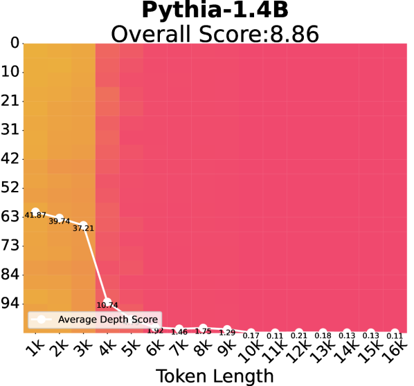
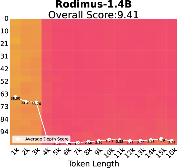
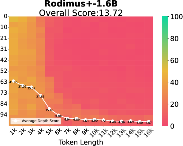
Figure 5: Results on NeedleBench. The average accuracy of each subtask of NeedleBench in contexts of different lengths. Overall Score represents the global average score.

4.3 Ablation Studies

In this section, we summarize the key conclusions from our ablation studies. A detailed analysis is provided in Appendix E.6. (i) Our assessment of the components in Rodimus reveals that the inclusion of ${\bm{g}}_{t}$, ${\bm{\tau}}_{t}$, and $\hat{\bm{\beta}}_{t}$ is crucial for the DDTS framework. However, the incorporation of ${\bm{\beta}}_{t}$ tends to complicate the training process, leading to suboptimal results. Additionally, the two-hop residual connection is beneficial as the model depth increases. (ii) In terms of head compression methods, we find that SKA offers a balanced compromise between GQA and MHA, delivering superior performance compared to GQA while utilizing fewer parameters relative to MHA, irrespective of the backbone models used. (iii) We have determined that the optimal hyperparameter values are $\ell=16$ and $n=64$. Notably, the Rodimus configuration with $n=64$ operates with a state size that is only half that of Mamba2, yet it outperforms Mamba2 on various benchmarks.

5 Conclusion

In this paper, we introduce Rodimus* (comprising Rodimus and Rodimus$+$), two innovative models that utilize semantic, token, and head compression. Experimental results demonstrate that Rodimus* effectively breaks the accuracy-efficiency trade-off in LLMs.

Appendix A Future Work

Rodimus* has delivered excellent results across benchmarks; however, there are areas for improvement. Due to limited computing resources, we have not expanded its parameters to match open-source models like RWKV6-14B and Qwen2-72B. Additionally, Rodimus* lacks the highly I/O-aware optimization found in models such as Mamba and Mamba2. There’s potential to enhance its performance by designing I/O-aware multi-head scalar decay and integrating it with Rodimus’s DDTS to broaden gating mechanisms without significantly impacting training efficiency. Furthermore, for Rodimus$+$, the memory usage of SW-SKA can be further reduced while achieving better practical application performance. We aim to address these issues in future work.

Appendix B Main Notation Introduction

Table 3: Meanings of Notations

Notation	Size	Meaning
$T$	Constant	The length of the context.
$d$	Constant	The model dimension.
$m$	Constant	The dimensionality of the hidden state corresponding to the token mixer.
$n$	Constant	The expansion factor of matrix hidden state, when is set to 1 in vector hidden state.
$d_{h}$	Constant	The head dimension in the multi-head mechanism.
$\mathbf{1}_{x}$	$1\times x$	The all-ones vector of dimension $x$.
${\bm{X}}$	$T\times d$	The input sequence of module.
${\bm{O}}$	$T\times d$	The output sequence of module.
${\bm{Q}}$	$T\times n$	The query.
${\bm{K}}$	$T\times n$	The key.
${\bm{V}}$	$T\times m$	The value.
${\bm{W}}_{Q}$	$d\times n$	The weight matrix of the query.
${\bm{W}}_{K}$	$d\times n$	The weight matrix of the key.
${\bm{W}}_{V}$	$d\times m$	The weight matrix of the value.
${\bm{S}}_{t}$	$n\times m$	The hidden state at stamp $t$.
${\bm{A}}_{t}$	$n\times m$	The transition matrix at stamp $t$.
${\bm{B}}_{t}$	$n\times m$	The input matrix at stamp $t$.
${\bm{C}}_{t}$	$1\times n$	The output matrix at stamp $t$.
${\bm{\alpha}}_{t}$	$1\times n$	The gating mechanism along the dimension $n$ acts on the transition.
$\hat{\bm{\alpha}}_{t}$	$1\times n$	The gating mechanism along the dimension $n$ acts on the input, which is negatively correlated with ${\bm{\alpha}}_{t}$.
${\bm{\beta}}_{t}$	$1\times m$	The gating mechanism along the dimension $m$ acts on the transition.
$\hat{\bm{\beta}}_{t}$	$1\times m$	The gating mechanism along the dimension $m$ acts on the input, which is negatively correlated with ${\bm{\beta}}_{t}$.
${\bm{u}}_{t}$	$n\times m$	The input term of recurrent calculations.
${\bm{x}}_{t}^{\prime}$	$1\times m$	The output of $\mathrm{ShortConv}$.
${\bm{g}}_{t}$	Variable	The gating mechanism of selection or decay. In Rodimus, it’s a selection gate with the size of $1\times n$.
${\bm{W}}_{g}$	$m\times n$	The weight matrix of ${\bm{g}}_{t}$.
${\bm{b}}_{g}$	$1\times n$	The bias of ${\bm{g}}_{t}$.
${\bm{\tau}}_{t}$	$1\times n$	The temperature gate in Rodimus.
${\bm{W}}_{\tau}$	$m\times n$	The weight matrix of ${\bm{\tau}}_{t}$ in Rodimus.
${\bm{b}}_{\tau}$	$1\times n$	The bias of ${\bm{\tau}}_{t}$ in Rodimus.
$\ell$	Constant	The low-rank dimensionality of projections.
${\bm{W}}_{\hat{\beta}}^{1}$	$m\times\ell$	The down-projection weight matrix of $\hat{\bm{\beta}}_{t}$ in Rodimus.
${\bm{W}}_{\hat{\beta}}^{2}$	$\ell\times m$	The up-projection weight matrix of $\hat{\bm{\beta}}_{t}$ in Rodimus.
${\bm{b}}_{\hat{\beta}}$	$1\times m$	The bias of $\hat{\bm{\beta}}_{t}$ in Rodimus.
${\bm{d}}_{t}$	$1\times m$	The feedthrough matrix in SSMs.

Appendix C Method Details

C.1 Similar functional forms of other methods

We summarize the functional forms of ${\bm{A}}_{t}$ and ${\bm{B}}_{t}$ used in state-of-the-art methods in Table 4.

Table 4: Comparison of ${\bm{A}}_{t}$ and ${\bm{B}}_{t}$ across various models. For models employing the multi-head mechanism, only the gates for a single head are presented. The term "Gate Dim" represents the dimensionality of the gates ${\bm{g}}_{t}$ in ${\bm{A}}_{t}$ and ${\bm{B}}_{t}$, and "L.A." denotes linear attention without scaling [3, 18]. Elements with the subscript $t$ are data-dependent gates, with most elements being learnable. Notably, the non-learnable constants include $\gamma$ in RetNet, $\tau$ in GLA and gRetNet, and $c$ in Hawk. Although the "State Size" of RWKV6 is smaller than that of Rodimus, the use of DDTS in Rodimus yields superior performance across all metrics (see Tables 2 and 14).

Model	Gate Dim	State Size $n\times m$	Parallelization like L.A.	Recurrent Type	${\bm{A}}_{t}$	${\bm{B}}_{t}$
L.A. [3]	No Gates	$256\times d$	✓	No Gates	$\mathbf{1}_{n}^{\top}\mathbf{1}_{m}$	$\mathbf{1}_{n}^{\top}\mathbf{1}_{m}$
RetNet [19]	$1\times 1$	$256\times d$	✓	Decay	$g\cdot\mathbf{1}_{n}^{\top}\mathbf{1}_{m}$	$\mathbf{1}_{n}^{\top}\mathbf{1}_{m}$
gRetNet [22]	$1\times 1$	$256\times d$	✓	Decay	$\big{(}\sigma(g_{t})^{1/\tau}\big{)}\cdot\mathbf{1}_{n}^{\top}\mathbf{1}_{m}$	$\mathbf{1}_{n}^{\top}\mathbf{1}_{m}$
GLA [9]	$1\times n$	$256\times d$	✓	Decay	$\big{(}\sigma({\bm{g}}_{t})^{1/\tau}\big{)}^{\top}\mathbf{1}_{m}$	$\mathbf{1}_{n}^{\top}\mathbf{1}_{m}$
RWKV6 [51]	$1\times n$	$64\times d$	✓	Decay	$\exp\big{(}-\exp({\bm{g}}_{t})\big{)}^{\top}\mathbf{1}_{m}$	$\mathbf{1}_{n}^{\top}\mathbf{1}_{m}$
HGRN2 [8]	$1\times n$	$128\times d$	✓	Selection	$\big{(}1-\sigma({\bm{g}}_{t})\big{)}^{\top}\mathbf{1}_{m}$	$\big{(}\sigma({\bm{g}}_{t})\big{)}^{\top}\mathbf{1}_{m}$
Hawk [20]	$1\times d$	$1\times d$	✗	Selection	$\sqrt{1-(a^{c\cdot\sigma({\bm{g}}_{t})})^{2}}$	$a^{c\cdot\sigma({\bm{g}}_{t})}$
S4D [52]	$1\times d$	$16\times d$	✗	Selection	$\exp(-{\bm{A}}\odot\mathbf{1}_{n}^{\top}{\bm{g}})$	$\mathbf{1}_{n}^{\top}\zeta({\bm{g}})$
Mamba [4]	$1\times d$	$16\times 2d$	✗	Selection	$\exp(-{\bm{A}}\odot\mathbf{1}_{n}^{\top}{\bm{g}}_{t})$	$\mathbf{1}_{n}^{\top}\zeta({\bm{g}}_{t})$
Mamba2 [5]	$1\times 1$	$128\times 2d$	✓	Selection	$\exp(-a\cdot g_{t})\cdot\mathbf{1}_{n}^{\top}\mathbf{1}_{m}$	$\zeta(g_{t})\cdot\mathbf{1}_{n}^{\top}\mathbf{1}_{m}$
Rodimus	$1\times n$	$64\times 2d$	✓	DDTS	$\exp(-{\bm{g}}_{t}\odot{\bm{\tau}}_{t})^{\top}\mathbf{1}_{m}$	$({\bm{g}}_{t}^{{\bm{\tau}}_{t}})^{\top}\mathbf{1}_{m}$

C.2 Related Work

Linear Attention with Gates: Linear attention replaces the traditional exponential kernel, $\exp({\bm{q}}_{t}^{\top}{\bm{k}}_{t})$, with the dot-product feature map $\phi({\bm{q}}_{t})^{\top}\phi({\bm{k}}_{t})$ [3]. This approach allows inference to be reformulated as a linear RNN with a matrix hidden state. However, without gating mechanisms, it often struggles to effectively capture input and forget historical information, resulting in irrelevant information within the hidden state [53]. To address this, gating mechanisms such as purely decay (e.g., GLA [9]) and selection mechanisms for associating input and decay (e.g., HGRN2 [8]) have been introduced.

These improvements, however, often lead to the issue of sacrificing hidden state size to enhance performance [8], lacking thorough analysis and design of gates, which hinders performance even with larger hidden states. In Section 3.1.1, we analyze effective gate design and propose a solution for a more efficient gating mechanism named DDTS.

State-Space Models: Recent advancements in state-space models based on HiPPO [54] have led to notable results in long sequence modeling, inspiring further work like S4 [55], S5 [56], and H3 [57]. Mamba [4] builds on S4D [52], the parameterized diagonal version of S4, making state-space model (SSM) parameters data-dependent. Its input-based selection mechanism arises from ZOH discretization. However, Mamba’s diagonal state space structure limits calculations with larger hidden states expanded by the expansion factor $n$, restricting memory capacity improvement.

Mamba2 [5] addresses this by using a scalar state space structure instead of the original diagonal state space structure in Mamba. This change allows Mamba2 to be trained with chunkwise parallelization, similar to linear attention [19, 58], permitting an expansion factor of 128. However, this approach mirrors linear attention’s challenge of over-relying on hidden state size while neglecting gating design. The oversimplified gating mechanism struggles to approximate the original softmax attention performance (see Section 3.1.1).

Our method features a similar architecture to Mamba2, enabling chunk-wise parallel calculations, while our gating mechanism, DDTS, better approximates softmax attention.

Softmax Attention with Custom Attention Mask: Several studies have enhanced the attention mechanism while retaining the softmax function. One approach involves modifying the attention scope by integrating prior knowledge to create diverse custom attention masks. During inference, these masks function similarly to token-level sequence compression, storing unmasked tokens in the KV cache [11]. Many studies observe local behavior in attention, leading to the use of local attention instead of full attention, as seen in models like LongFormer [24]. Additionally, some methods employ learnable patterns, such as the Routing Transformer [59], to construct attention masks in a data-driven manner. However, custom attention masks only support token-level compression, which can result in information loss for masked tokens.

In Rodimus$+$, the Rodimus block can compress long contexts and transform token embeddings into context embeddings by dynamically fusing multiple tokens to create semantic compression, as shown in Figure 2b. This enables the local attention in SW-SKA to capture token information beyond the window.

C.3 Chunkwise Parallel Representation of the Rodimus Block

Let $\bm{{\mathcal{A}}}_{t}=\prod^{t}_{j=1}{\bm{\alpha}}_{j}$ denote the cumulative product of gates ${\bm{\alpha}}_{j}$, and define $\bm{{\mathcal{A}}}=\{\bm{{\mathcal{A}}}_{1},\dots,\bm{{\mathcal{A}}}_{T}\}\in\mathbb{R}^{T\times n}$, then ${\bm{\Lambda}}_{t}=\prod^{t}_{j=1}{\bm{\beta}}_{j}$ denote the cumulative product of gates ${\bm{\beta}}_{j}$, and define ${\bm{\Lambda}}=\{{\bm{\Lambda}}_{1},\dots,{\bm{\Lambda}}_{T}\}\in\mathbb{R}^{T\times m}$. After the following derivation, we can obtain the parallel form of the Rodimus block:

$${\bm{S}}_{t} =({\bm{\alpha}}_{t}^{\top}{\bm{\beta}}_{t})\odot{\bm{S}}_{t-1}+(\hat{\bm{\alpha}}_{t}^{\top}\hat{\bm{\beta}}_{t})\odot({\bm{k}}_{t}^{\top}{\bm{v}}_{t})$$ (14)

$$=({\bm{\alpha}}_{t}^{\top}{\bm{\beta}}_{t})\odot{\bm{S}}_{t-1}+(\hat{\bm{\alpha}}_{t}\odot{\bm{k}}_{t})^{\top}(\hat{\bm{\beta}}_{t}\odot{\bm{v}}_{t}),$$

$${\bm{o}}_{t} ={\bm{q}}_{t}{\bm{S}}_{t},$$

from the derivation in [9], we can have:

$${\bm{o}}_{t} ={\bm{q}}_{t}\sum^{t}_{i=1}\big{(}\prod^{t}_{j=i+1}({\bm{\alpha}}_{j}^{\top}{\bm{\beta}}_{j})\odot(\hat{\bm{\alpha}}_{i}\odot{\bm{k}}_{i})^{\top}(\hat{\bm{\beta}}_{i}\odot{\bm{v}}_{i})\big{)}$$ (15)

$$={\bm{q}}_{t}\sum^{t}_{i=1}\big{(}(\prod^{t}_{j=i+1}{\bm{\alpha}}_{j})^{\top}(\prod^{t}_{j=i+1}{\bm{\beta}}_{j})\odot(\hat{\bm{\alpha}}_{i}\odot{\bm{k}}_{i})^{\top}(\hat{\bm{\beta}}_{i}\odot{\bm{v}}_{i})\big{)}$$

$$={\bm{q}}_{t}\sum^{t}_{i=1}\big{(}(\prod^{t}_{j=i+1}{\bm{\alpha}}_{j}\odot{\bm{k}}_{i}\odot\hat{\bm{\alpha}}_{i})^{\top}(\prod^{t}_{j=i+1}{\bm{\beta}}_{j}\odot{\bm{v}}_{i}\odot\hat{\bm{\beta}}_{i})\big{)}$$

$$=\sum_{i=1}^{t}\bigg{[}{\bm{q}}_{t}\big{(}\prod_{j=i+1}^{t}{\bm{\alpha}}_{j}\odot\hat{\bm{\alpha}}_{i}\odot{\bm{k}}_{i}\big{)}^{\top}\bigg{]}\big{(}\prod_{j=i+1}^{t}{\bm{\beta}}_{j}\odot\hat{\bm{\beta}}_{i}\odot{\bm{v}}_{i}\big{)}$$

$$=\sum_{i=1}^{t}\bigg{[}\big{(}{\bm{q}}_{t}\odot\bm{{\mathcal{A}}}_{t}\big{)}\big{(}\hat{\bm{\alpha}}_{i}\odot{\bm{k}}_{i}/\bm{{\mathcal{A}}}_{i}\big{)}^{\top}\bigg{]}\big{(}\hat{\bm{\beta}}_{i}\odot{\bm{v}}_{i}/{\bm{\Lambda}}_{i}\big{)}\odot{\bm{\Lambda}}_{t},$$

$$\tilde{{\bm{Q}}} ={\bm{Q}}\odot\bm{{\mathcal{A}}},\quad\tilde{{\bm{K}}}={\bm{K}}/\bm{{\mathcal{A}}}\odot\hat{\bm{\alpha}},\quad\tilde{{\bm{V}}}={\bm{V}}/\bm{\Lambda}\odot\hat{\bm{\beta}},$$ (16)

$${\bm{O}} =(\tilde{{\bm{Q}}}\tilde{{\bm{K}}}^{\top}\odot{\bm{M}})\tilde{{\bm{V}}},$$

$$\tilde{{\bm{O}}} ={\bm{O}}\odot\bm{\Lambda}.$$

It follows from Eq. (16) that the parallel formula can be written as:

$$\tilde{{\bm{O}}}=\big{(}({\bm{Q}}\odot\bm{{\mathcal{A}}})({\bm{K}}/\bm{{\mathcal{A}}}\odot\hat{\bm{\alpha}})^{\top}\odot{\bm{M}}\big{)}({\bm{V}}/\bm{\Lambda}\odot\hat{\bm{\beta}})\odot\bm{\Lambda}.$$ (17)

Since we set $\beta_{j}=1$ in Section 3.1.1, the above equation can be simplified as:

$${\bm{O}}=\big{(}({\bm{Q}}\odot\bm{{\mathcal{A}}})({\bm{K}}/\bm{{\mathcal{A}}}\odot\hat{\bm{\alpha}})^{\top}\odot{\bm{M}}\big{)}({\bm{V}}\odot\hat{\bm{\beta}}),$$ (18)

which the parallel form for the proposed Rodimus block. However, the complexity of computing ${\bm{O}}$ via Eq. (18) is quadratic. To further reduce the training complexity, we exploit a chunkwise integration of the recurrent and parallel forms, in analogy to other linear attention approaches [9]. Specifically, we first divide the entire sequence into $T/B$ consecutive chunks, each with length $B$. For each chunk, the parallel computation as described in Eq. (18) is employed to obtain the intra-chunk output ${\bm{O}}^{\mathrm{intra}}$. Subsequently, information between chunks is integrated using a recurrence approach akin to Eq. (11):

$${\bm{S}}_{[i]}={\bm{S}}_{[i-1]}\odot((\textstyle\prod^{iB}_{j=(i-1)B+1}{\bm{\alpha}}_{j})^{\top}\mathbf{1})+({\bm{K}}_{[i]}\odot\hat{\bm{\alpha}}_{[i]}\odot\textstyle\prod^{iB}_{j=(i-1)B+b+1}{\bm{\alpha}}_{j})^{\top}({\bm{V}}_{[i]}\odot\hat{\bm{\beta}}_{[i]}),$$

$${\bm{O}}_{[i]}^{\mathrm{inter}}=({\bm{Q}}_{[i]}\odot\textstyle\prod^{(i-1)B+b}_{j=(i-1)B+1}{\bm{\alpha}}_{j}){\bm{S}}_{[i]},$$ (19)

where $[i]$ represents the $i$-th chunk. The parallel computations within each chunk can further leverage tensor cores to speed up matrix operations [9, 5]. Additionally, this sequential form for inter-chunk computation reduces overall computational complexity from quadratic to subquadratic and optimizes memory utilization during training. To further optimize training efficiency, we incorporate FlashLinearAttention.

C.4 Rodimus$+$’s Relationship to Existing Hybrid Models

Here we focus on models that integrate self-attention with recurrent architectures. One notable approach is Griffin [20, 60], which combines sliding window attention with a linear RNN. However, unlike Rodimus$+$, which employs matrix hidden states, the hidden state in Griffin’s linear RNN is a vector, limiting its capacity to retain historical information. Another hybrid model, Based [61], also integrates linear attention and sliding window attention. Unfortunately, it lacks a decay or gating mechanism within its linear attention framework, making it susceptible to the attention dilution problem. On a different note, Samba [62] explores various methods to combine Mamba with self-attention. The original version of Samba inserts MLP (FFN) layers between Mamba and self-attention, which neglects Mamba’s channel mixing capabilities and introduces unnecessary parameters. Another variant of Samba, Mamba-SWA-MLP, then removes the MLP between Mamba and self-attention, but it does not implement the two-hop residual connection used in Rodimus$+$. Different from the aforementioned works, Mamba-2-Attention [5] seeks to enhance retrieval (i.e., recall) capabilities by replacing some of the SSM layers with self-attention. This approach contrasts with the model architecture of Rodimus$+$, which regularly incorporates SWA between SSM layers. Moreover, determining the optimal number of layers to replace with attention requires further experimentation, and the introduction of full attention layers with their quadratic complexity complicates model scaling. Lastly, Jamba [63] combines the Transformer block with Mamba and MoE layers, yet it also adds extra MLP layers after Mamba, similar to Samba. Additionally, establishing the optimal number of Transformer blocks remains an unresolved challenge.

C.5 Models in Experiments

Transformer [41]: The foundational architecture with a causal attention mask used in GPT-3.

Transformer$++$ [1]: An enhancement of the Transformer, Transformer$++$ incorporates RoPE, GLU, and RMSNorm for improved performance. It is currently the most robust and widely used Transformer configuration [4].

Mamba [4]: Mamba makes the original SSM parameters data-dependent and introduces an I/O-aware associative scan.

Mamba2 [5]: Mamba2 simplifies the diagonal state space structure in Mamba to the scalar state space structure, enhancing computational efficiency through chunkwise parallelism algorithms like linear attention.

GPT-Neo [64]: Similar to the Transformer, GPT-Neo employs full attention and local attention in alternating layers and uses ALiBi for positional encoding.

OPT [65]: OPT mirrors the Transformer architecture but utilizes learnable positional encoding.

BLOOM [66]: BLOOM is akin to the Transformer, except it uses ALiBi for positional encoding.

Pythia [67]: An improvement upon the Transformer, Pythia uses RoPE for positional encoding.

RWKV4 [7]: RWKV4 integrates techniques such as token-shift to merge RNN-like states with Transformer-style attention mechanisms.

RWKV6 [51]: An enhanced version of RWKV4, RWKV6 features a more flexible gating mechanism and introduces multi-headed matrix-valued states to boost the memory capacity of the recurrent model.

RetNet [19]: RetNet applies RoPE with a fixed scalar decay $\gamma$ to linear attention.

GLA [9]: GLA omits positional encoding on linear attention, opting instead for data-dependent decay.

HGRN [6]: HGRN introduces a decay lower bound based on traditional linear RNNs, employs recurrent calculation in the complex domain, and uses a selection mechanism in the real domain.

HGRN2 [8]: HGRN2 removes complex domain calculations from HGRN and introduces state expansion similar to Mamba2 and linear attention.

Qwen2 [68]: Built on Transformer$++$, Qwen2 uses GQA to reduce inference costs.

Llama3 [39]: Llama3’s architecture is similar to that of Qwen2.

Appendix D Proof

D.1 Lemma for Selection Mechanism

Lemma 1.

For the recurrent model defined below,

$${\bm{S}}_{t}=\phi_{A}(\bm{\eta}_{t})\odot{\bm{S}}_{t-1}+\phi_{B}(\bm{\eta}_{t})\odot{\bm{u}}_{t},$$ (20)

where ${\bm{S}}_{t}\in\mathbb{R}^{n\times m}$,${\bm{x}}_{t}\in\mathbb{R}^{1\times m}$,${\bm{u}}_{t}=\phi_{u}({\bm{x}}_{t})\in\mathbb{R}^{n\times m}$,$\bm{\eta}_{t}=\phi_{\eta}({\bm{x}}_{t})\in\mathbb{R}^{n\times m}$. If the following condition is met, it is a model with the selection mechanism.

$$\quad{\forall}i\in\{0,1,\dots,n\}\ {\forall}j\in\{0,1,\dots,m\},\frac{d\phi_{A}(\bm{\eta}_{t,i,j})}{d\bm{\eta}_{t,i,j}}\frac{d\phi_{B}(\bm{\eta}_{t,i,j})}{d\bm{\eta}_{t,i,j}}<0.$$ (21)

Proof.

Since the product of the gradient of $\phi_{A}(\bm{\eta}_{t,i,j})$ and $\phi_{B}(\bm{\eta}_{t,i,j})$ is negative, $\phi_{A}(\bm{\eta}_{t,i,j})$ is negatively correlated with $\phi_{B}(\bm{\eta}_{t,i,j})$, satisfying the selection mechanism.

∎

D.2 Proof of Proposition 1

To prove Proposition 1, we first verify that Rodimus satisfies Lemma 1. In Rodimus, ${\bm{u}}_{t}={\bm{k}}_{t}^{\top}{\bm{v}}_{t}$, and we define $\bm{\eta}_{t}=({\bm{x}}_{t}{\bm{W}}_{g}+{\bm{b}}_{g})^{\top}\mathbf{1}_{m}$. Consequently, ${\bm{g}}_{t}^{\prime}=\mathrm{softplus}(\bm{\eta}_{t})$. For simplicity, we omit temperature $\bm{\tau}_{t}^{\prime}$ in this proof. We define $\phi_{A}(\bm{\eta}_{t})=\exp(-{\bm{g}}_{t}^{\prime})$ and $\phi_{B}(\bm{\eta}_{t})={\bm{g}}_{t}^{\prime}$, which corresponds to Eq. (11). Finally, we find that:

$$\frac{d\phi_{A}(\bm{\eta}_{t,i,j})}{d\bm{\eta}_{t,i,j}}\frac{d\phi_{B}(\bm{\eta}_{t,i,j})}{d\bm{\eta}_{t,i,j}}=-\sigma(\bm{\eta}_{t,i,j})^{2}(1-\sigma(\bm{\eta}_{t,i,j}))<0,$$ (22)

where $\sigma$ is the sigmoid function. Thus, Rodimus satisfies the selection mechanism.

Appendix E Experimental Details

E.1 WikiText-103

The specific settings are listed in Table 5. The main difference from [6] is that we increase the total batch size, which reduces the training steps to obtain results more quickly.

Table 5: Settings details for WikiText-103 and the Pile subset.

Dataset	WikiText-103	Pile subset
Tokenizer method	BPE	GPT-Neox Tokenizer
Vocab size	50265	50277
Sequence length	512	2048
Total Batch size	256	256
Training steps	25000	13351
Warmup steps	2000	572
Peak learing rate	5e-4	5e-4
Min learning rate	1e-5	1e-5
Optimizer	AdamW	AdamW
Adam $\beta_{1}$	0.9	0.9
Adam $\beta_{2}$	0.95	0.95
Weight decay	0.1	0.1
Gradient clipping	1.0	1.0

E.2 Scaling Laws

We train all models on a subset of the Pile, using the parameter settings from GPT-3 [41]. The context length is 2048 tokens. The training steps and total token counts follow the Mamba settings [4]. Detailed configurations are provided in Table 6. For methods using purely recurrent models that combine GLU and token mixers, such as Mamba series and Rodimus, the number of layers should be doubled to match the GPT-3 specifications.

Table 6: Model parameters and training settings used in our scaling experiments. "Steps" indicates the number of training steps, and "Batch Size" refers to the number of tokens used for each update.

Params	n_layer	d_model	n_heads/d_head	Steps	Learing Rate	Batch Size	Tokens
125M	12	768	12/64	4800	6e-4	0.5M	2.5B
350M	24	1024	16/64	13500	3e-4	0.5M	7B
760M	24	1536	16/96	29000	2.5e-4	0.5M	15B
1.3B	24	2048	32/64	50000	2e-4	0.5M	26B

E.3 Downstream Evaluation

Our default training settings align with those in Table 6 of the scaling law experiment. Unless otherwise specified, these settings remain unchanged. All our models use mixed precision and FSDP [69] to improve training speed. To maximize GPU memory usage, we adjust the batch size according to Table 7 and modify the maximum and minimum learning rates.

The Rodimus Tokenizer uses Hugging Face’s byte-level BPE algorithm, featuring a vocabulary of 126,340 tokens, including special tokens, trained on a 60 billion token subset of the curated dataset.

Notably, we do not apply weight decay to the biases of linear projections and LayerNorm, nor to the weights of LayerNorm or RMSNorm. Additionally, we set the head size of SW-SKA in Rodimus$+$ to 128 and the window size to half the training context, as described in Samba [62].

Table 7: The extra training settings of Rodimus* in downstream task.

Params (B)	Tokenizer	Training context	Batch size	Max learning rate	Min learning rate
0.13	GPT-NeoX	2048	1.5M	3e-3	1e-5
0.46	Rodimus	2048	0.8M	1.5e-3	1e-5
1.4	Rodimus	2048	6.3M	1e-3	1e-5

E.4 MQAR (Multi-Query Associative Recall)

The MQAR task [16] is a benchmark widely used to assess the associative recall capabilities of recurrent models. In this task, input sequences consist of several key-value pairs followed by queries. When presented with a query, the model must retrieve the corresponding key-value pair from earlier in the sequence in order to accurately predict the next token.

For example, consider the input "A 3 B 2 C 1". The key-value pairs are "A 3", "B 2", and "C 1". Later, when "A ?", "B ?", and "C ?" appear as queries, the correct outputs are "3", "2", and "1", respectively.

Notably, models utilizing full softmax attention tend to achieve perfect scores on this benchmark. Consequently, our study concentrates exclusively on recurrent models, specifically Mamba [4], Mamba2 [5], RWKV [7], and RWKV6 [51].

The experiment in Figure 6 follows the settings from MQAR [16]. We use sequence lengths of 128, 256, and 512, with corresponding key-value pairs of 8, 16, and 32. The total vocabulary size is set to 8192, the number of model layers to 2, and the model dimension $d$ varies as 64, 128, 256, and 512. Learning rates of $10^{-4}$, $10^{-3.3}$, $10^{-2.7}$ and $10^{-2}$ are applied to train for 64 epochs using the cosine annealing learning rate schedule, with the best accuracy recorded as the reported accuracy for each model dimension. In Figure 1(b), the sequence length is increased to 1024, the key-value pairs are set to 256, and the model dimension $d$ is fixed at 256. Only the expansion factor $n$ is varied. Learning rates of $10^{-2}$, $10^{-2.5}$ and $10^{-3.5}$ are used to train for 32 epochs with the cosine annealing learning rate schedule, and the best accuracy is recorded as the reported accuracy corresponding to the expansion factor.

We first depict the accuracy as a function of the expansion factor $n$ in Figure 1(b). In this analysis, we focus on the Mamba series for comparison, as their architecture closely resembles that of Rodimus*, allowing for consistent settings across all models. Our results indicate that Rodimus* exhibits superior recall ability at the same expansion factor $n$. This enhancement can be attributed to the model’s DDTS mechanism, which filters out irrelevant past information and current inputs more effectively.

Next, we present the accuracy as a function of model dimension $d$ in Figure 6, where the expansion factor $n$ is maintained at its original value across different models. Once again, Rodimus* achieves the highest performance. In comparison, Mamba and RWKV underperform, particularly when the model dimension is small. This suggests that the fixed-capacity state of these models can only deliver reliable recall results when the state size is sufficiently large to retain relevant past information.

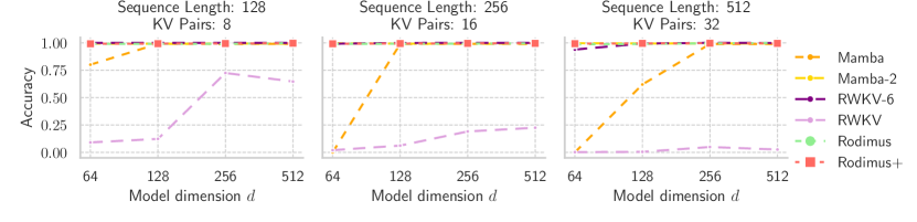
Figure 6: Recall accuracy of MQAR Task at different sequence lengths.

E.5 NeedleBench

The NeedleBench [70] is a retrieval evaluation method that randomly inserts key information into long texts to create prompts for LLMs. The primary objective of this test is to assess the ability of LLMs to effectively extract crucial information from extensive documents, thereby evaluating their proficiency in processing and comprehending long-form content. The NeedleBench comprises several tasks: the Single-Needle Retrieval Task (S-RT), the Multi-Needle Retrieval Task (M-RT), the Multi-Needle Reasoning Task (M-RS), and the Ancestry Trace Challenge (ATC). The S-RT focuses on the precise extraction of specific details, while the M-RT evaluates the retrieval of multiple related pieces of information, simulating complex queries. The M-RS task involves synthesizing and understanding interconnected information, and the ATC examines logical reasoning, requiring comprehensive engagement with all provided content to solve intricate problems.

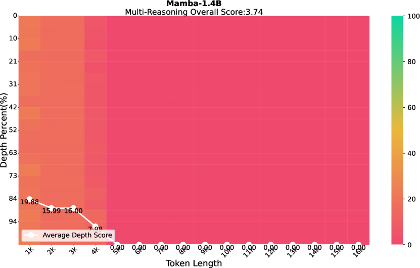
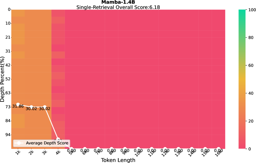
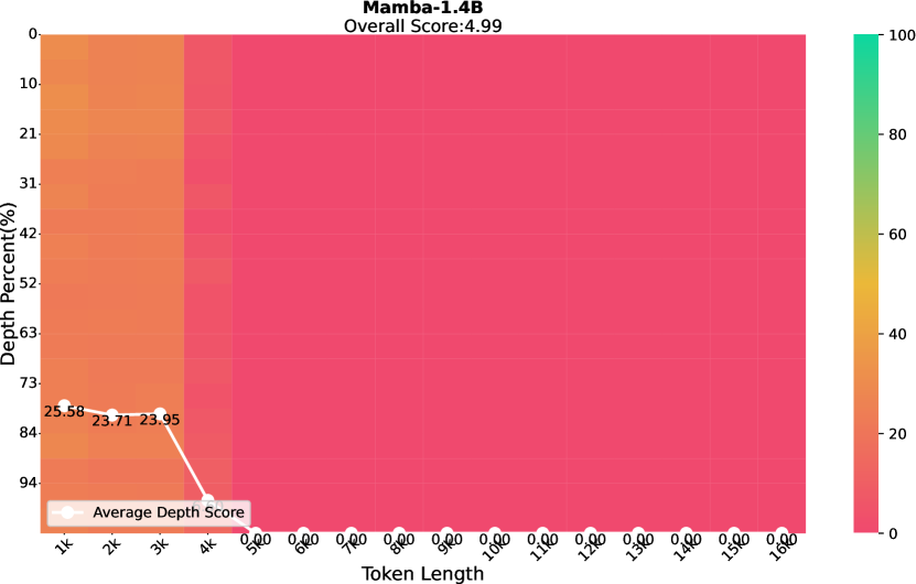
Figure 9: Mamba-1.4B

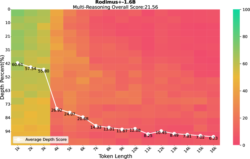
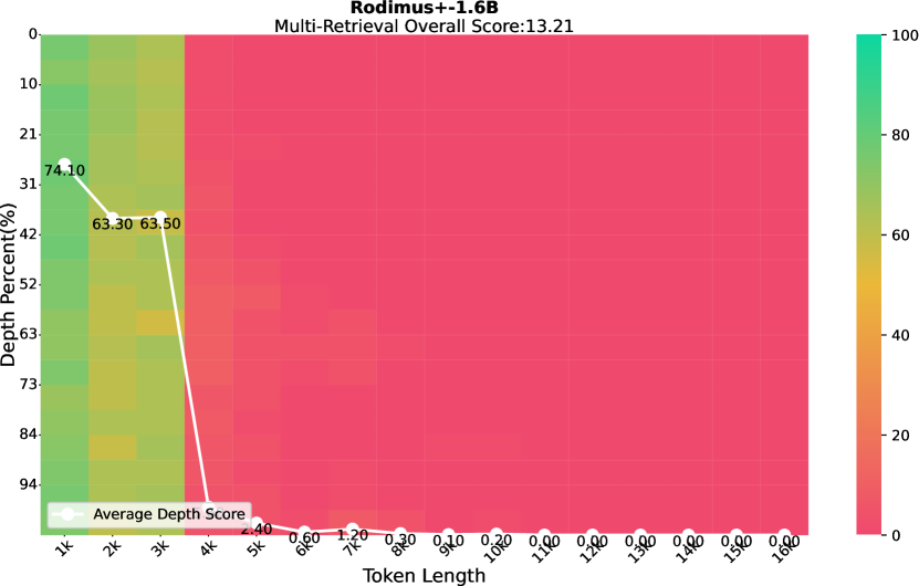
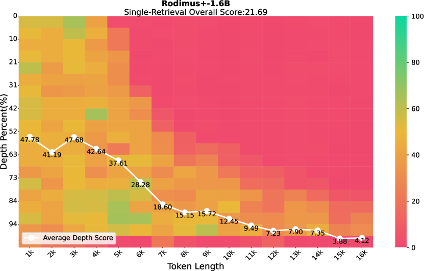
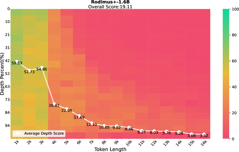
Figure 14: Rodimus$+$-1.6B-4K

In this study, we evaluate Mamba-1.4B [4], Mamba2-1.3B [5], Pythia-1.4B [67], Rodimus-1.4B, and Rodimus$+$-1.6B on NeedleBench using OpenCompass [71], since the sequence length of all these models is 2048 tokens. The brief evaluation results, featuring Mamba2-1.3B, Pythia-1.4B, Rodimus-1.4B, and Rodimus$+$-1.6B, are presented in Figure 5. Full evaluation results, including subtasks, are detailed in Figures 9 (Mamba-1.4B), 10 (Mamba2-1.3B), 11 (Rodimus-1.4B), 12 (Pythia-1.4B), and 13 (Rodimus$+$-1.6B). The "Overall Score" represents the average result of these subtasks. Additionally, we present the NeedleBench results for Rodimus$+$ in Appendix F.2, where the model trained on a longer context demonstrates superior long-distance retrieval capabilities, as shown in Figure 14.

Many studies have suggested that pre-trained recurrent models tend to underperform on challenging recall-intensive tasks like NeedleBench when compared to models utilizing full attention mechanisms [57, 17]. This trend is illustrated by comparisons between Pythia and Mamba2. Nevertheless, Rodimus demonstrates superior recall ability relative to Pythia. While Pythia shines in scenarios involving shorter contexts (0k-4k), Rodimus exhibits better extrapolation capabilities for longer contexts, leading to overall enhanced performance. Furthermore, Rodimus$+$, a hybrid model, further improves recall ability by integrating global semantic-level and local token-level representations. The results for Rodimus and Rodimus$+$ indicate that the Rodimus family effectively navigates the accuracy-efficiency trade-off, particularly in terms of enhancing recall ability. In addition, training with longer contexts can effectively enhance the model’s recall ability in Needlebench. Rodimus$+$ trained with the 4K-length context performs better on Needlebench than when trained with the standard 2K-length context.

E.6 Ablation Studies Details

In this section, we present ablation studies designed to achieve two primary objectives: (i) assessing the contributions of various components—such as the gates and the two-hop residual—in Rodimus*, (ii) evaluating performance with different head compression methods, and (iii) determining the optimal hyperparameter values ($\ell$ and $n$). We begin with experiments conducted on the WikiText-103 dataset, chosen for its relatively small size, which allows for quicker results and makes the impact of removing specific components easily observable. The second set of experiments utilizes a 7B subset of Pile, providing a larger dataset to discern subtle differences arising from hyperparameter adjustments. For the WikiText-103 dataset, we report both the test PPL and the best test PPL. The test PPL refers to the evaluation of the test set after training on the training dataset for a fixed number of epochs, while the best test PPL reflects the lowest value achieved during early stopping of training. Although the former approach is commonly employed in the literature, it does not always accurately capture model performance.

The necessity of ${\bm{g}}_{t}$, ${\bm{\tau}}_{t}$, and $\hat{\bm{\beta}}_{t}$: As presented in Table 11, the removal of these gates results in decreased performance, indicating their essential role in DDTS.

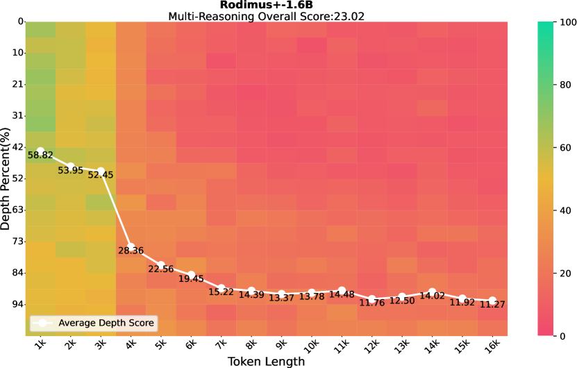
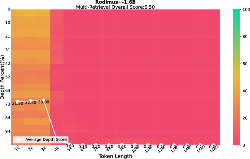
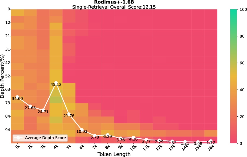
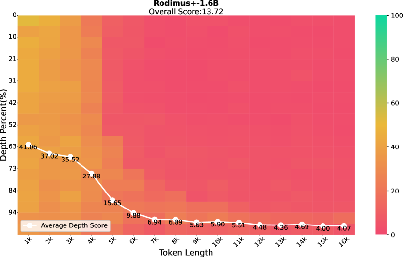
Figure 13: Rodimus$+$-1.6B-2K

The necessity of ${\bm{\beta}}_{t}$: Table 11 shows that incorporating $\hat{\bm{\beta}}_{t}$ does not reduce the PPL further; in fact, it tends to increase it slightly. As shown in Figure 13, this finding suggests that excluding ${\bm{\beta}}_{t}$, is preferable, as it does not provide performance improvements but may complicate the training process and hinder the training efficiency (see detailed explanations Section 3.1.1).

The necessity of the two-hop residual: According to Table 13, the two-hop residual in Rodimus$+$ can slightly enhance performance when the model deepens with more layers. This mechanism aids in stabilizing training, as noted by [36]. Given that modern Large Language Models (LLMs) typically consist of many layers and the two-hop residual incurs no extra computational cost, we implement it in Rodimus$+$.

Comparison between SKA, GQA, and MHA: Table 11 indicates that SKA consistently outperforms GQA in terms of PPL across both Rodimus$+$ or Transformer$++$, demonstrating the effectiveness of SKA. However, SKA performs less optimally than MHA, likely due to increased training difficulty, requiring more iterations or data for comparable performance. Nevertheless, since SKA is more parameter-efficient than MHA and surpasses GQA in performance, we opt to utilize SKA in Rodimus$+$.

Sensitivity to $\ell$ and $n$: Table 9 reveals that increasing the rank $\ell$ of the weight matrices in Eq. (10) generally improves performance but also raises the parameter count. We find that setting $\ell=16$ effectively balances performance and parameter quantity, and thus we adopt this value for our experiments. Regarding the state expansion factor $n$, shown in Table 9, we observe that valid PPL decreases as $n$ increases; however, the rate of decrease slows significantly for $n\geq 64$. Consequently, we establish $n=64$ for our experiments. Note that $n=128$ in Mamba2. Thus, Rodimus outperforms Mamba2 in most tests with only half the state size.

Table 8: Results of the ablation experiments on the low-rank term.

$\ell$	Valid PPL	Params (M)	Valid PPL	Params (M)
1	7.41	126.3	5.84	360.8
2	7.32	126.4	5.81	361.0
4	7.36	126.5	5.77	361.4
8	7.30	126.8	5.76	362.2
16	7.26	127.4	5.75	363.7
32	7.31	128.6	5.74	366.9
64	7.24	130.9	5.71	373.2
128	7.17	135.7	5.70	385.8

Table 9: Results of ablation experiments on expansion factor $n$.

$n$	Valid PPL	Params (M)	Valid PPL	Params (M)
16	5.75	363.7	7.26	127.4
32	5.66	370.0	7.13	129.8
64	5.62	382.6	7.01	134.5
128	5.58	407.8	6.95	143.9
256	5.57	458.1	6.9	162.8

Table 10: Results of ablation experiment of MHA, GQA and SKA.

Model	Head Type	Valid PPL
Transformer$++$	MHA	7.25
Transformer$++$	GQA	7.38
Transformer$++$	SKA	7.33
Rodimus$+$	MHA	7.09
Rodimus$+$	GQA	7.19
Rodimus$+$	SKA	7.15

Table 11: Results of ablation experiments on gates.

$\hat{\bm{\beta}}_{t}$	${\bm{g}}_{t}$	$\bm{\tau}_{t}$	Test PPL	Best Test PPL
✗	✗	✗	23.23	22.66
✓	✗	✗	23.24	22.20
✗	✓	✗	22.34	21.33
✗	✓	✓	22.14	21.15
✓	✓	✗	22.24	21.17
✓	✓	✓	21.90	20.84

Table 12: Results of ablation experiment on type of ${\bm{\beta}}$.

${\bm{\beta}}_{t}=?$	Test PPL	Best Test PPL
$\prod^{t}_{j=i+1}{\bm{\beta}}_{j}$	24.36	23.32
$\mathbf{1}_{m}$	23.24	22.20

Table 13: Results of ablation experiment on models with or without two-hop residual. "THR" denotes the two-hop residual, and $L$ represents the number of layers.

$L$	THR	Test PPL	Best Test PPL
6	✓	21.56	20.46
6	✗	21.77	20.37
24	✓	21.50	20.85
24	✗	21.52	20.95

Appendix F More Experimental Results

F.1 Gates with Temperature $\tau_{t}$

We further visualize the effect of gates influenced by the temperature gate ${\bm{\tau}}_{t}$. In Figure 7, we present the curves of the decay term $\exp({\bm{g}}_{t}\odot{\bm{\tau}}_{t})$ and the input term ${\bm{g}}_{t}^{{\bm{\tau}}_{t}}$ as the temperature varies. As ${\bm{\tau}}_{t}$ decreases, the lower bounds of both terms gradually rise, enhancing information retention.

In Figure 8, we compare the gates of a layer in models from Table 11 with and without the temperature gate ${\bm{\tau}}_{t}$. By comparing Figure 8(a) with Figure 8(b), and Figure 8(c) with Figure 8(d), we observe that the inclusion of temperature increases the flexibility of the gates in selecting information.

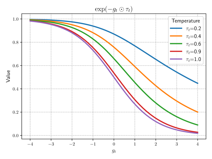
(a) Decay term.

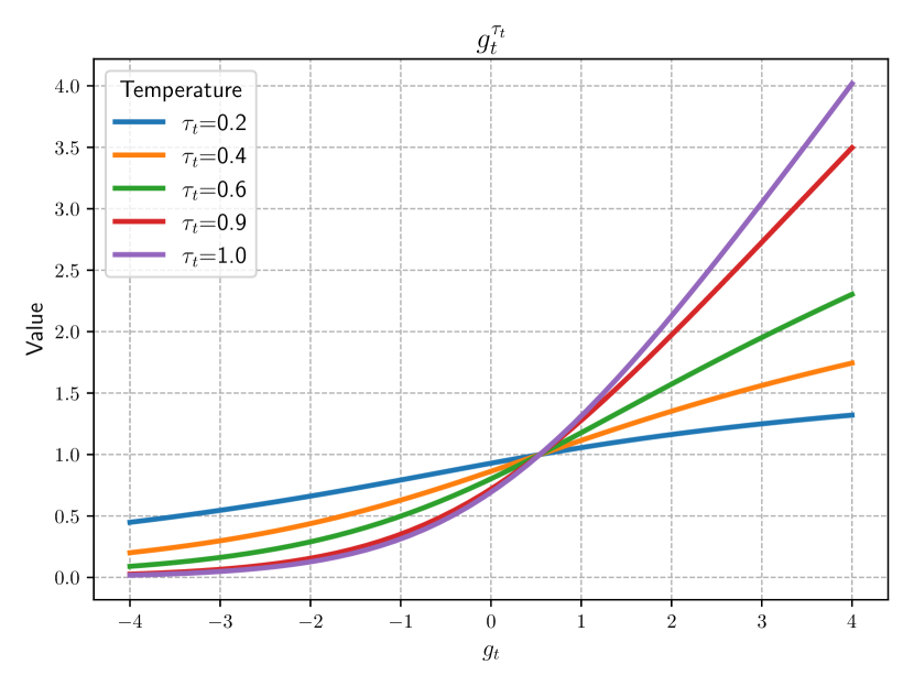
(b) Input term.

Figure 7: The curves of the gates with temperature gate ${\bm{\tau}}_{t}$.

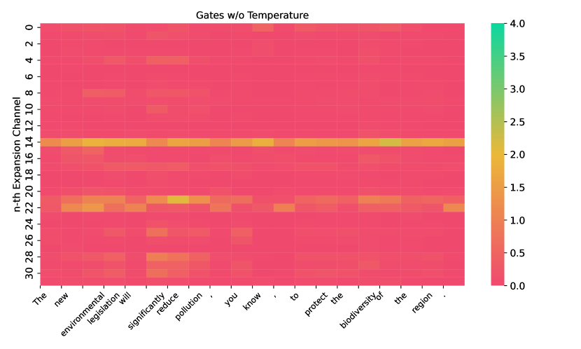
(a) Input w/o $\tau$.

(b) Input w $\tau$.

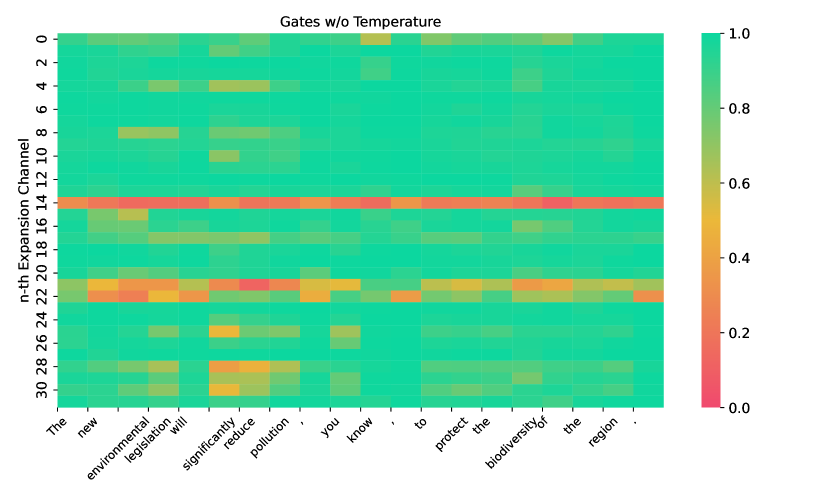
(c) Decay w/o $\tau$.

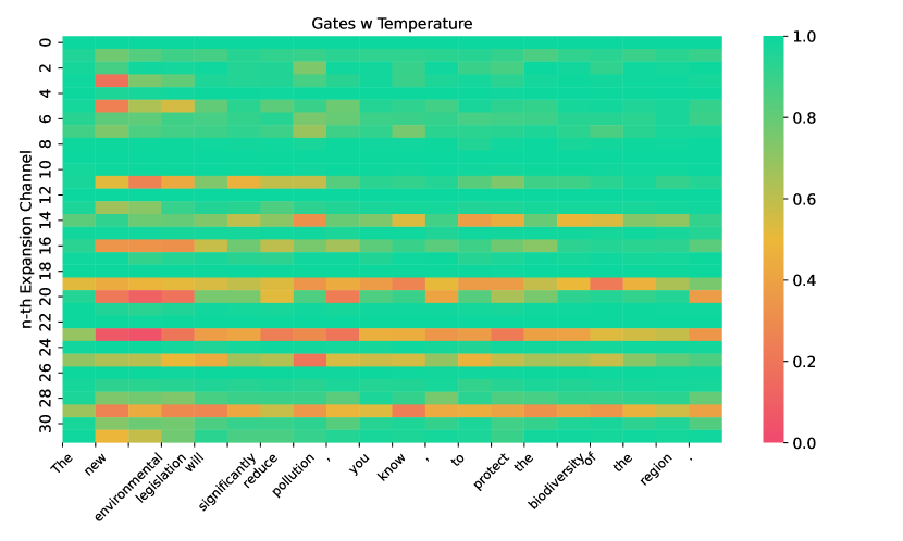
(d) Decay w $\tau$.

Figure 8: The visualization results of the gates are shown. The y-axis represents the n-th dimension of the gates, and the x-axis displays the sub-words after tokenization. (a) and (b) show the heatmap visualizations of the input gate ${\bm{g}}_{t}$ and ${\bm{g}}_{t}^{\tau_{t}}$. (c) and (d) present the corresponding results of $\exp({\bm{g}}_{t})$ and $\exp({\bm{g}}_{t}\odot\tau_{t})$.

F.2 More Practical LLM: Multi-stage training of Rodimus$+$

To enhance the practical capabilities of Rodimus$+$ and develop it into a functional LLM, we train it using multi-stage training, similar to Llama3 [39], with a focus on math and code. We increase the total number of tokens to 2.5 trillion and extend the context length to 4096 tokens.

We compare Rodimus$+$, after multi-stage training, with popular open-source models using the OpenCompass framework. These models include Gemma2-2B [72], Qwen2-1.5B [68], RWKV6-1.6B [51], and Llama3.2-1.2B [39]. The evaluation benchmarks encompass a wide range of fields, including code (HumanEval (0-shot) [73], MBPP (0-shot) [74]), math (GSM8K (4-shot) [75], MATH (4-shot) [76]), and other few-shot benchmarks (C-Eval (5-shot) [77], MMLU (5-shot) [78], CMMLU (5-shot) [79], BBH (3-shot) [80]).

The results are presented in Table 14. Rodimus$+$-1.6B, trained on 2.5 trillion tokens, outperforms Gemma2-2B, which is trained on the same amount of tokens. Its performance is comparable to Qwen2-1.5B, trained on 7 trillion tokens, and even surpasses Llama3.2-1.2B, which is trained on over 9 trillion tokens. Additionally, it excels beyond RWKV6-1.6B, a recurrent model with fixed-size hidden states.

Notably, Rodimus$+$ performs exceptionally well in math and code tasks with the memory complexity of ${\mathcal{O}}(1)$. In contrast, Qwen2-1.5B, Gemma2-2B, and Llama3.2-1.2B are attention-based models with the memory complexity ${\mathcal{O}}(T)$. Rodimus$+$ offers the potential for low-cost deployment on edge devices, enabling a broader range of applications, such as local code assistants.

Table 14: Evaluation on Practical Benchmarks.

Model	Params	Tokens	HumanEval	MBPP	GSM8K	MATH	C-Eval	CMMLU	MMLU	BBH	AVG
Rodimus$+$	1.6B	2.5T	32.93	34	51.25	16.94	58.77	56.1	49.11	45.66	44.55
Gemma2	2B	2.5T	17.7	29.6	23.9	12.76	39.44	39.04	51.3	41.9	33.99
Qwen2	1.5B	7T	35.37	31.6	49.2	15.9	68.44	68.23	56.18	33.84	46.2
RWKV6	1.6B	1.4T	0	1	3.56	0.92	24.3	24.8	26.42	23.81	14.97
Llama3.2	1.2B	>9T	18.9	22.8	8.34	2.24	27.56	27.13	32.22	30.62	21.56

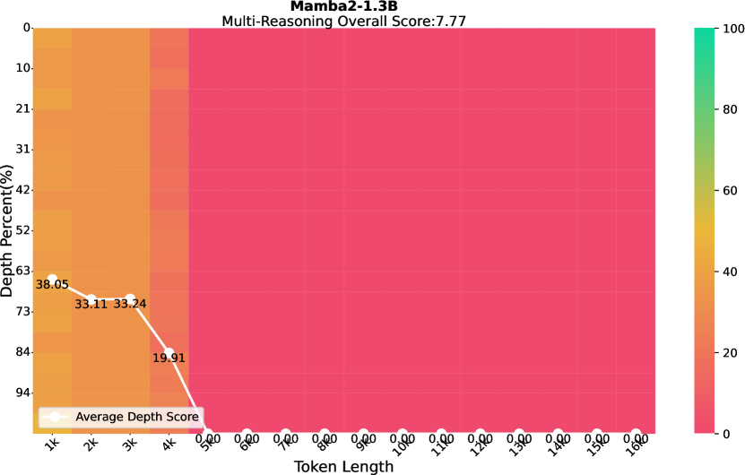
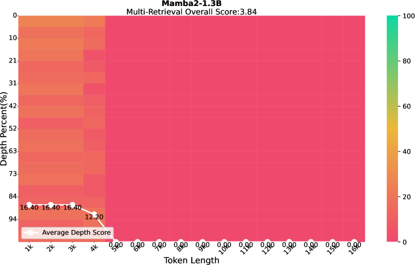
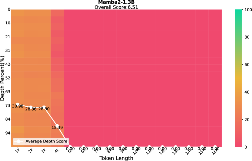
Figure 10: Mamba2-1.3B

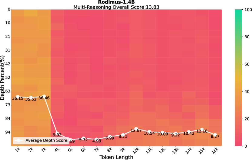
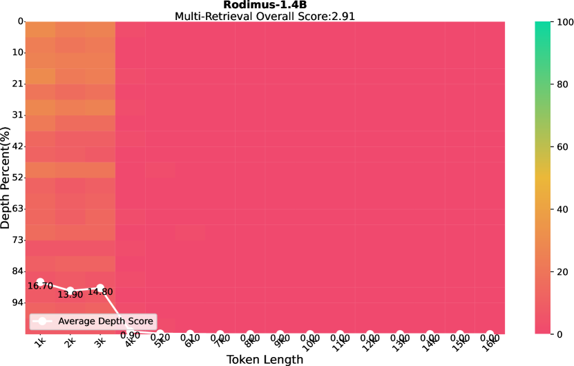
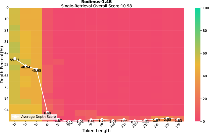
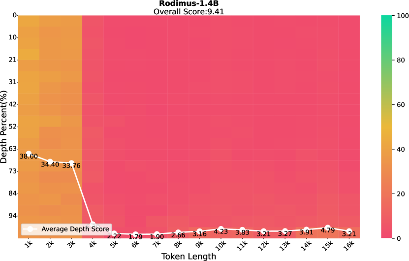
Figure 11: Rodimus-1.4B

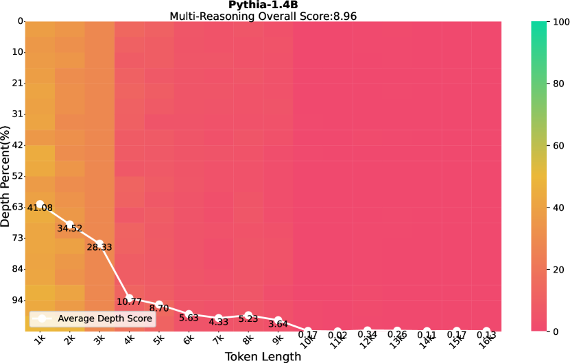
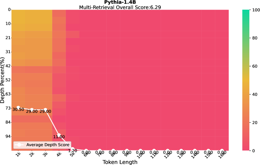
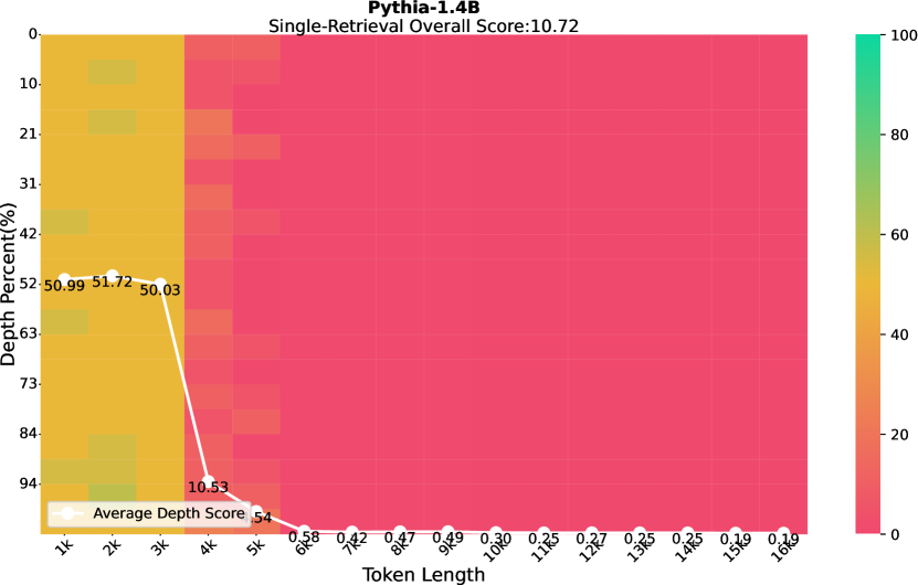
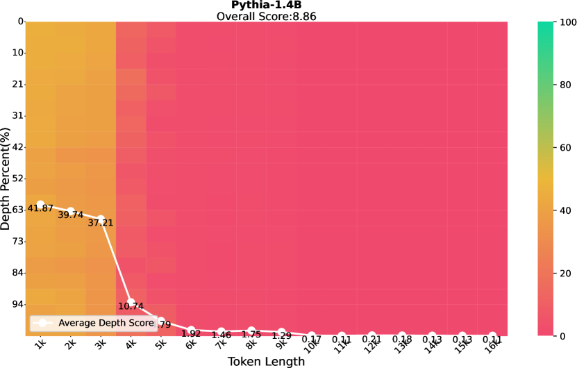
Figure 12: Pythia-1.4B

References

- [1] Hugo Touvron, Thibaut Lavril, Gautier Izacard, Xavier Martinet, Marie-Anne Lachaux, Timothée Lacroix, Baptiste Rozière, Naman Goyal, Eric Hambro, Faisal Azhar, et al. Llama: Open and efficient foundation language models. arXiv preprint arXiv:2302.13971, 2023.
- [2] Régis Pierrard Ilyas Moutawwakil. Llm-perf leaderboard. https://huggingface.co/spaces/optimum/llm-perf-leaderboard, 2023.
- [3] Angelos Katharopoulos, Apoorv Vyas, Nikolaos Pappas, and François Fleuret. Transformers are rnns: Fast autoregressive transformers with linear attention. In International conference on machine learning, pages 5156–5165. PMLR, 2020.
- [4] Albert Gu and Tri Dao. Mamba: Linear-time sequence modeling with selective state spaces. arXiv preprint arXiv:2312.00752, 2023.
- [5] Tri Dao and Albert Gu. Transformers are SSMs: Generalized models and efficient algorithms through structured state space duality. In International Conference on Machine Learning (ICML), 2024.
- [6] Zhen Qin, Songlin Yang, and Yiran Zhong. Hierarchically gated recurrent neural network for sequence modeling. Advances in Neural Information Processing Systems, 36, 2024.
- [7] Bo Peng, Eric Alcaide, Quentin Anthony, Alon Albalak, Samuel Arcadinho, Stella Biderman, Huanqi Cao, Xin Cheng, Michael Chung, Leon Derczynski, Xingjian Du, Matteo Grella, Kranthi Gv, Xuzheng He, Haowen Hou, Przemyslaw Kazienko, Jan Kocon, Jiaming Kong, Bartłomiej Koptyra, Hayden Lau, Jiaju Lin, Krishna Sri Ipsit Mantri, Ferdinand Mom, Atsushi Saito, Guangyu Song, Xiangru Tang, Johan Wind, Stanisław Woźniak, Zhenyuan Zhang, Qinghua Zhou, Jian Zhu, and Rui-Jie Zhu. RWKV: Reinventing RNNs for the transformer era. In Houda Bouamor, Juan Pino, and Kalika Bali, editors, Findings of the Association for Computational Linguistics: EMNLP 2023, pages 14048–14077, Singapore, December 2023. Association for Computational Linguistics.
- [8] Zhen Qin, Songlin Yang, Weixuan Sun, Xuyang Shen, Dong Li, Weigao Sun, and Yiran Zhong. HGRN2: Gated linear RNNs with state expansion. In First Conference on Language Modeling, 2024.
- [9] Songlin Yang, Bailin Wang, Yikang Shen, Rameswar Panda, and Yoon Kim. Gated linear attention transformers with hardware-efficient training. In Forty-first International Conference on Machine Learning, 2024.
- [10] Songlin Yang, Bailin Wang, Yu Zhang, Yikang Shen, and Yoon Kim. Parallelizing linear transformers with the delta rule over sequence length. arXiv preprint arXiv:2406.06484, 2024.
- [11] Guangxuan Xiao, Yuandong Tian, Beidi Chen, Song Han, and Mike Lewis. Efficient streaming language models with attention sinks. In The Twelfth International Conference on Learning Representations, 2024.
- [12] Chi Han, Qifan Wang, Hao Peng, Wenhan Xiong, Yu Chen, Heng Ji, and Sinong Wang. Lm-infinite: Zero-shot extreme length generalization for large language models. In Proceedings of the 2024 Conference of the North American Chapter of the Association for Computational Linguistics: Human Language Technologies (Volume 1: Long Papers), pages 3991–4008, 2024.
- [13] Noam Shazeer. Fast transformer decoding: One write-head is all you need, 2019.
- [14] Joshua Ainslie, James Lee-Thorp, Michiel de Jong, Yury Zemlyanskiy, Federico Lebron, and Sumit Sanghai. GQA: Training generalized multi-query transformer models from multi-head checkpoints. In Houda Bouamor, Juan Pino, and Kalika Bali, editors, Proceedings of the 2023 Conference on Empirical Methods in Natural Language Processing, pages 4895–4901, Singapore, December 2023. Association for Computational Linguistics.
- [15] A Vaswani. Attention is all you need. Advances in Neural Information Processing Systems, 2017.
- [16] Simran Arora, Sabri Eyuboglu, Aman Timalsina, Isys Johnson, Michael Poli, James Zou, Atri Rudra, and Christopher Re. Zoology: Measuring and improving recall in efficient language models. In The Twelfth International Conference on Learning Representations, 2024.
- [17] Roger Waleffe, Wonmin Byeon, Duncan Riach, Brandon Norick, Vijay Korthikanti, Tri Dao, Albert Gu, Ali Hatamizadeh, Sudhakar Singh, Deepak Narayanan, et al. An empirical study of mamba-based language models. arXiv preprint arXiv:2406.07887, 2024.
- [18] Zhen Qin, Xiaodong Han, Weixuan Sun, Dongxu Li, Lingpeng Kong, Nick Barnes, and Yiran Zhong. The devil in linear transformer. In Proceedings of the 2022 Conference on Empirical Methods in Natural Language Processing, pages 7025–7041, 2022.
- [19] Yutao Sun, Li Dong, Shaohan Huang, Shuming Ma, Yuqing Xia, Jilong Xue, Jianyong Wang, and Furu Wei. Retentive network: A successor to transformer for large language models. arXiv preprint arXiv:2307.08621, 2023.
- [20] Soham De, Samuel L Smith, Anushan Fernando, Aleksandar Botev, George Cristian-Muraru, Albert Gu, Ruba Haroun, Leonard Berrada, Yutian Chen, Srivatsan Srinivasan, et al. Griffin: Mixing gated linear recurrences with local attention for efficient language models. arXiv preprint arXiv:2402.19427, 2024.
- [21] Zhen Qin, Weixuan Sun, Hui Deng, Dongxu Li, Yunshen Wei, Baohong Lv, Junjie Yan, Lingpeng Kong, and Yiran Zhong. cosformer: Rethinking softmax in attention. In International Conference on Learning Representations, 2022.
- [22] Yutao Sun, Li Dong, Yi Zhu, Shaohan Huang, Wenhui Wang, Shuming Ma, Quanlu Zhang, Jianyong Wang, and Furu Wei. You only cache once: Decoder-decoder architectures for language models, 2024.
- [23] Rewon Child, Scott Gray, Alec Radford, and Ilya Sutskever. Generating long sequences with sparse transformers. arXiv preprint arXiv:1904.10509, 2019.
- [24] Iz Beltagy, Matthew E. Peters, and Arman Cohan. Longformer: The long-document transformer. arXiv:2004.05150, 2020.
- [25] Daya Guo, Canwen Xu, Nan Duan, Jian Yin, and Julian McAuley. Longcoder: A long-range pre-trained language model for code completion. In International Conference on Machine Learning, pages 12098–12107. PMLR, 2023.
- [26] Yutao Sun, Li Dong, Barun Patra, Shuming Ma, Shaohan Huang, Alon Benhaim, Vishrav Chaudhary, Xia Song, and Furu Wei. A length-extrapolatable transformer. In Anna Rogers, Jordan Boyd-Graber, and Naoaki Okazaki, editors, Proceedings of the 61st Annual Meeting of the Association for Computational Linguistics (Volume 1: Long Papers), pages 14590–14604, Toronto, Canada, July 2023. Association for Computational Linguistics.
- [27] Ofir Press, Noah Smith, and Mike Lewis. Train short, test long: Attention with linear biases enables input length extrapolation. In International Conference on Learning Representations, 2022.
- [28] Jianlin Su, Yu Lu, Shengfeng Pan, Bo Wen, and Yunfeng Liu. Roformer: Enhanced transformer with rotary position embedding, 2021.
- [29] Liliang Ren, Yang Liu, Shuohang Wang, Yichong Xu, Chenguang Zhu, and Cheng Xiang Zhai. Sparse modular activation for efficient sequence modeling. Advances in Neural Information Processing Systems, 36:19799–19822, 2023.
- [30] Imanol Schlag, Tsendsuren Munkhdalai, and Jürgen Schmidhuber. Learning associative inference using fast weight memory. In International Conference on Learning Representations, 2021.
- [31] Nicolas Papernot, Abhradeep Thakurta, Shuang Song, Steve Chien, and Úlfar Erlingsson. Tempered sigmoid activations for deep learning with differential privacy. In Proceedings of the AAAI Conference on Artificial Intelligence, volume 35, pages 9312–9321, 2021.
- [32] Fengjun Wang, Sarai Mizrachi, Moran Beladev, Guy Nadav, Gil Amsalem, Karen Lastmann Assaraf, and Hadas Harush Boker. Mumic–multimodal embedding for multi-label image classification with tempered sigmoid. In Proceedings of the AAAI Conference on Artificial Intelligence, volume 37, pages 15603–15611, 2023.
- [33] Edward J Hu, Yelong Shen, Phillip Wallis, Zeyuan Allen-Zhu, Yuanzhi Li, Shean Wang, Lu Wang, and Weizhu Chen. LoRA: Low-rank adaptation of large language models. In International Conference on Learning Representations, 2022.
- [34] Yann N Dauphin, Angela Fan, Michael Auli, and David Grangier. Language modeling with gated convolutional networks. In International conference on machine learning, pages 933–941. PMLR, 2017.
- [35] Weizhe Hua, Zihang Dai, Hanxiao Liu, and Quoc Le. Transformer quality in linear time. In International conference on machine learning, pages 9099–9117. PMLR, 2022.
- [36] Xuezhe Ma, Xiaomeng Yang, Wenhan Xiong, Beidi Chen, Lili Yu, Hao Zhang, Jonathan May, Luke Zettlemoyer, Omer Levy, and Chunting Zhou. Megalodon: Efficient llm pretraining and inference with unlimited context length, 2024.
- [37] Biao Zhang and Rico Sennrich. Root mean square layer normalization. Advances in Neural Information Processing Systems, 32, 2019.
- [38] Stephen Merity, Caiming Xiong, James Bradbury, and Richard Socher. Pointer sentinel mixture models. In International Conference on Learning Representations, 2022.
- [39] Abhimanyu Dubey, Abhinav Jauhri, Abhinav Pandey, Abhishek Kadian, Ahmad Al-Dahle, Aiesha Letman, Akhil Mathur, Alan Schelten, Amy Yang, Angela Fan, et al. The llama 3 herd of models. arXiv preprint arXiv:2407.21783, 2024.
- [40] Jordan Hoffmann, Sebastian Borgeaud, Arthur Mensch, Elena Buchatskaya, Trevor Cai, Eliza Rutherford, Diego de Las Casas, Lisa Anne Hendricks, Johannes Welbl, Aidan Clark, et al. An empirical analysis of compute-optimal large language model training. Advances in Neural Information Processing Systems, 35:30016–30030, 2022.
- [41] Tom Brown, Benjamin Mann, Nick Ryder, Melanie Subbiah, Jared D Kaplan, Prafulla Dhariwal, Arvind Neelakantan, Pranav Shyam, Girish Sastry, Amanda Askell, et al. Language models are few-shot learners. Advances in neural information processing systems, 33:1877–1901, 2020.
- [42] Leo Gao, Stella Biderman, Sid Black, Laurence Golding, Travis Hoppe, Charles Foster, Jason Phang, Horace He, Anish Thite, Noa Nabeshima, Shawn Presser, and Connor Leahy. The Pile: An 800gb dataset of diverse text for language modeling. arXiv preprint arXiv:2101.00027, 2020.
- [43] Denis Paperno, Germán Kruszewski, Angeliki Lazaridou, Ngoc Quan Pham, Raffaella Bernardi, Sandro Pezzelle, Marco Baroni, Gemma Boleda, and Raquel Fernández. The LAMBADA dataset: Word prediction requiring a broad discourse context. In Katrin Erk and Noah A. Smith, editors, Proceedings of the 54th Annual Meeting of the Association for Computational Linguistics (Volume 1: Long Papers), pages 1525–1534, Berlin, Germany, August 2016. Association for Computational Linguistics.
- [44] Yonatan Bisk, Rowan Zellers, Ronan Le Bras, Jianfeng Gao, and Yejin Choi. Piqa: Reasoning about physical commonsense in natural language. In Thirty-Fourth AAAI Conference on Artificial Intelligence, 2020.
- [45] Rowan Zellers, Ari Holtzman, Yonatan Bisk, Ali Farhadi, and Yejin Choi. Hellaswag: Can a machine really finish your sentence? In Proceedings of the 57th Annual Meeting of the Association for Computational Linguistics, 2019.
- [46] Keisuke Sakaguchi, Ronan Le Bras, Chandra Bhagavatula, and Yejin Choi. Winogrande: An adversarial winograd schema challenge at scale. arXiv preprint arXiv:1907.10641, 2019.
- [47] Todor Mihaylov, Peter Clark, Tushar Khot, and Ashish Sabharwal. Can a suit of armor conduct electricity? a new dataset for open book question answering. In EMNLP, 2018.
- [48] Peter Clark, Isaac Cowhey, Oren Etzioni, Tushar Khot, Ashish Sabharwal, Carissa Schoenick, and Oyvind Tafjord. Think you have solved question answering? try arc, the ai2 reasoning challenge. ArXiv, abs/1803.05457, 2018.
- [49] Leo Gao, Jonathan Tow, Baber Abbasi, Stella Biderman, Sid Black, Anthony DiPofi, Charles Foster, Laurence Golding, Jeffrey Hsu, Alain Le Noac’h, Haonan Li, Kyle McDonell, Niklas Muennighoff, Chris Ociepa, Jason Phang, Laria Reynolds, Hailey Schoelkopf, Aviya Skowron, Lintang Sutawika, Eric Tang, Anish Thite, Ben Wang, Kevin Wang, and Andy Zou. A framework for few-shot language model evaluation, 12 2023.
- [50] Guilherme Penedo, Hynek Kydlíček, Anton Lozhkov, Margaret Mitchell, Colin Raffel, Leandro Von Werra, Thomas Wolf, et al. The fineweb datasets: Decanting the web for the finest text data at scale. arXiv preprint arXiv:2406.17557, 2024.
- [51] Bo Peng, Daniel Goldstein, Quentin Anthony, Alon Albalak, Eric Alcaide, Stella Biderman, Eugene Cheah, Teddy Ferdinan, Haowen Hou, Przemysław Kazienko, et al. Eagle and finch: Rwkv with matrix-valued states and dynamic recurrence. arXiv preprint arXiv:2404.05892, 2024.
- [52] Albert Gu, Karan Goel, Ankit Gupta, and Christopher Ré. On the parameterization and initialization of diagonal state space models. Advances in Neural Information Processing Systems, 35:35971–35983, 2022.
- [53] Jos Van Der Westhuizen and Joan Lasenby. The unreasonable effectiveness of the forget gate. arXiv preprint arXiv:1804.04849, 2018.
- [54] Albert Gu, Tri Dao, Stefano Ermon, Atri Rudra, and Christopher Ré. Hippo: Recurrent memory with optimal polynomial projections. Advances in neural information processing systems, 33:1474–1487, 2020.
- [55] Albert Gu, Karan Goel, and Christopher Ré. Efficiently modeling long sequences with structured state spaces. In The International Conference on Learning Representations (ICLR), 2022.
- [56] Jimmy T.H. Smith, Andrew Warrington, and Scott Linderman. Simplified state space layers for sequence modeling. In The Eleventh International Conference on Learning Representations, 2023.
- [57] Daniel Y. Fu, Tri Dao, Khaled K. Saab, Armin W. Thomas, Atri Rudra, and Christopher Ré. Hungry Hungry Hippos: Towards language modeling with state space models. In International Conference on Learning Representations, 2023.
- [58] Xuezhe Ma, Chunting Zhou, Xiang Kong, Junxian He, Liangke Gui, Graham Neubig, Jonathan May, and Zettlemoyer Luke. Mega: Moving average equipped gated attention. arXiv preprint arXiv:2209.10655, 2022.
- [59] Aurko Roy, Mohammad Saffar, Ashish Vaswani, and David Grangier. Efficient content-based sparse attention with routing transformers. Transactions of the Association for Computational Linguistics, 9:53–68, 2021.
- [60] Aleksandar Botev, Soham De, Samuel L Smith, Anushan Fernando, George-Cristian Muraru, Ruba Haroun, Leonard Berrada, Razvan Pascanu, Pier Giuseppe Sessa, Robert Dadashi, et al. Recurrentgemma: Moving past transformers for efficient open language models. arXiv preprint arXiv:2404.07839, 2024.
- [61] Simran Arora, Sabri Eyuboglu, Michael Zhang, Aman Timalsina, Silas Alberti, James Zou, Atri Rudra, and Christopher Re. Simple linear attention language models balance the recall-throughput tradeoff. In ICLR 2024 Workshop on Mathematical and Empirical Understanding of Foundation Models, 2024.
- [62] Liliang Ren, Yang Liu, Yadong Lu, Yelong Shen, Chen Liang, and Weizhu Chen. Samba: Simple hybrid state space models for efficient unlimited context language modeling. arXiv preprint arXiv:2406.07522, 2024.
- [63] Opher Lieber, Barak Lenz, Hofit Bata, Gal Cohen, Jhonathan Osin, Itay Dalmedigos, Erez Safahi, Shaked Meirom, Yonatan Belinkov, Shai Shalev-Shwartz, et al. Jamba: A hybrid transformer-mamba language model. arXiv preprint arXiv:2403.19887, 2024.
- [64] Sid Black, Leo Gao, Phil Wang, Connor Leahy, and Stella Biderman. GPT-Neo: Large Scale Autoregressive Language Modeling with Mesh-Tensorflow, March 2021. If you use this software, please cite it using these metadata.
- [65] Susan Zhang, Stephen Roller, Naman Goyal, Mikel Artetxe, Moya Chen, Shuohui Chen, Christopher Dewan, Mona Diab, Xian Li, Xi Victoria Lin, et al. Opt: Open pre-trained transformer language models. arXiv preprint arXiv:2205.01068, 2022.
- [66] Teven Le Scao, Angela Fan, Christopher Akiki, Ellie Pavlick, Suzana Ilić, Daniel Hesslow, Roman Castagné, Alexandra Sasha Luccioni, François Yvon, Matthias Gallé, et al. Bloom: A 176b-parameter open-access multilingual language model. 2023.
- [67] Stella Biderman, Hailey Schoelkopf, Quentin Gregory Anthony, Herbie Bradley, Kyle O’Brien, Eric Hallahan, Mohammad Aflah Khan, Shivanshu Purohit, USVSN Sai Prashanth, Edward Raff, et al. Pythia: A suite for analyzing large language models across training and scaling. In International Conference on Machine Learning, pages 2397–2430. PMLR, 2023.
- [68] An Yang, Baosong Yang, Binyuan Hui, Bo Zheng, Bowen Yu, Chang Zhou, Chengpeng Li, Chengyuan Li, Dayiheng Liu, Fei Huang, et al. Qwen2 technical report. arXiv preprint arXiv:2407.10671, 2024.
- [69] Yanli Zhao, Andrew Gu, Rohan Varma, Liang Luo, Chien-Chin Huang, Min Xu, Less Wright, Hamid Shojanazeri, Myle Ott, Sam Shleifer, et al. Pytorch fsdp: experiences on scaling fully sharded data parallel. arXiv preprint arXiv:2304.11277, 2023.
- [70] Mo Li, Songyang Zhang, Yunxin Liu, and Kai Chen. Needlebench: Can llms do retrieval and reasoning in 1 million context window?, 2024.
- [71] OpenCompass Contributors. Opencompass: A universal evaluation platform for foundation models. https://github.com/open-compass/opencompass, 2023.
- [72] Gemma Team, Morgane Riviere, Shreya Pathak, Pier Giuseppe Sessa, Cassidy Hardin, Surya Bhupatiraju, Léonard Hussenot, Thomas Mesnard, Bobak Shahriari, Alexandre Ramé, et al. Gemma 2: Improving open language models at a practical size. arXiv preprint arXiv:2408.00118, 2024.
- [73] Mark Chen, Jerry Tworek, Heewoo Jun, Qiming Yuan, Henrique Ponde De Oliveira Pinto, Jared Kaplan, Harri Edwards, Yuri Burda, Nicholas Joseph, Greg Brockman, et al. Evaluating large language models trained on code. arXiv preprint arXiv:2107.03374, 2021.
- [74] Jacob Austin, Augustus Odena, Maxwell Nye, Maarten Bosma, Henryk Michalewski, David Dohan, Ellen Jiang, Carrie Cai, Michael Terry, Quoc Le, et al. Program synthesis with large language models. arXiv preprint arXiv:2108.07732, 2021.
- [75] Karl Cobbe, Vineet Kosaraju, Mohammad Bavarian, Mark Chen, Heewoo Jun, Lukasz Kaiser, Matthias Plappert, Jerry Tworek, Jacob Hilton, Reiichiro Nakano, et al. Training verifiers to solve math word problems. arXiv preprint arXiv:2110.14168, 2021.
- [76] Dan Hendrycks, Collin Burns, Saurav Kadavath, Akul Arora, Steven Basart, Eric Tang, Dawn Song, and Jacob Steinhardt. Measuring mathematical problem solving with the math dataset. NeurIPS, 2021.
- [77] Yuzhen Huang, Yuzhuo Bai, Zhihao Zhu, Junlei Zhang, Jinghan Zhang, Tangjun Su, Junteng Liu, Chuancheng Lv, Yikai Zhang, Jiayi Lei, Yao Fu, Maosong Sun, and Junxian He. C-eval: A multi-level multi-discipline chinese evaluation suite for foundation models. In Advances in Neural Information Processing Systems, 2023.
- [78] Dan Hendrycks, Collin Burns, Steven Basart, Andy Zou, Mantas Mazeika, Dawn Song, and Jacob Steinhardt. Measuring massive multitask language understanding. Proceedings of the International Conference on Learning Representations (ICLR), 2021.
- [79] Haonan Li, Yixuan Zhang, Fajri Koto, Yifei Yang, Hai Zhao, Yeyun Gong, Nan Duan, and Timothy Baldwin. Cmmlu: Measuring massive multitask language understanding in chinese, 2023.
- [80] Mirac Suzgun, Nathan Scales, Nathanael Schärli, Sebastian Gehrmann, Yi Tay, Hyung Won Chung, Aakanksha Chowdhery, Quoc Le, Ed Chi, Denny Zhou, et al. Challenging big-bench tasks and whether chain-of-thought can solve them. In Findings of the Association for Computational Linguistics: ACL 2023, pages 13003–13051, 2023.