The Sampling-Gaussian for stereo matching

Abstract

The soft-argmax operation is widely adopted in neural network-based stereo matching methods to enable differentiable regression of disparity. However, network trained with soft-argmax is prone to being multimodal due to absence of explicit constraint to the shape of the probability distribution. Previous methods leverages Laplacian distribution and cross-entropy for training but failed to effectively improve the accuracy and even compromises the efficiency of the network. In this paper, we conduct a detailed analysis of the previous distribution-based methods and propose a novel supervision method for stereo matching, Sampling-Gaussian. We sample from the Gaussian distribution for supervision. Moreover, we interpret the training as minimizing the distance in vector space and propose a combined loss of L1 loss and cosine similarity loss. Additionally, we leveraged bilinear interpolation to upsample the cost volume. Our method can be directly applied to any soft-argmax-based stereo matching method without a reduction in efficiency. We have conducted comprehensive experiments to demonstrate the superior performance of our Sampling-Gaussian. The experimental results prove that we have achieved better accuracy on five baseline methods and two datasets. Our method is easy to implement, and the code is available online.

1 Introduction

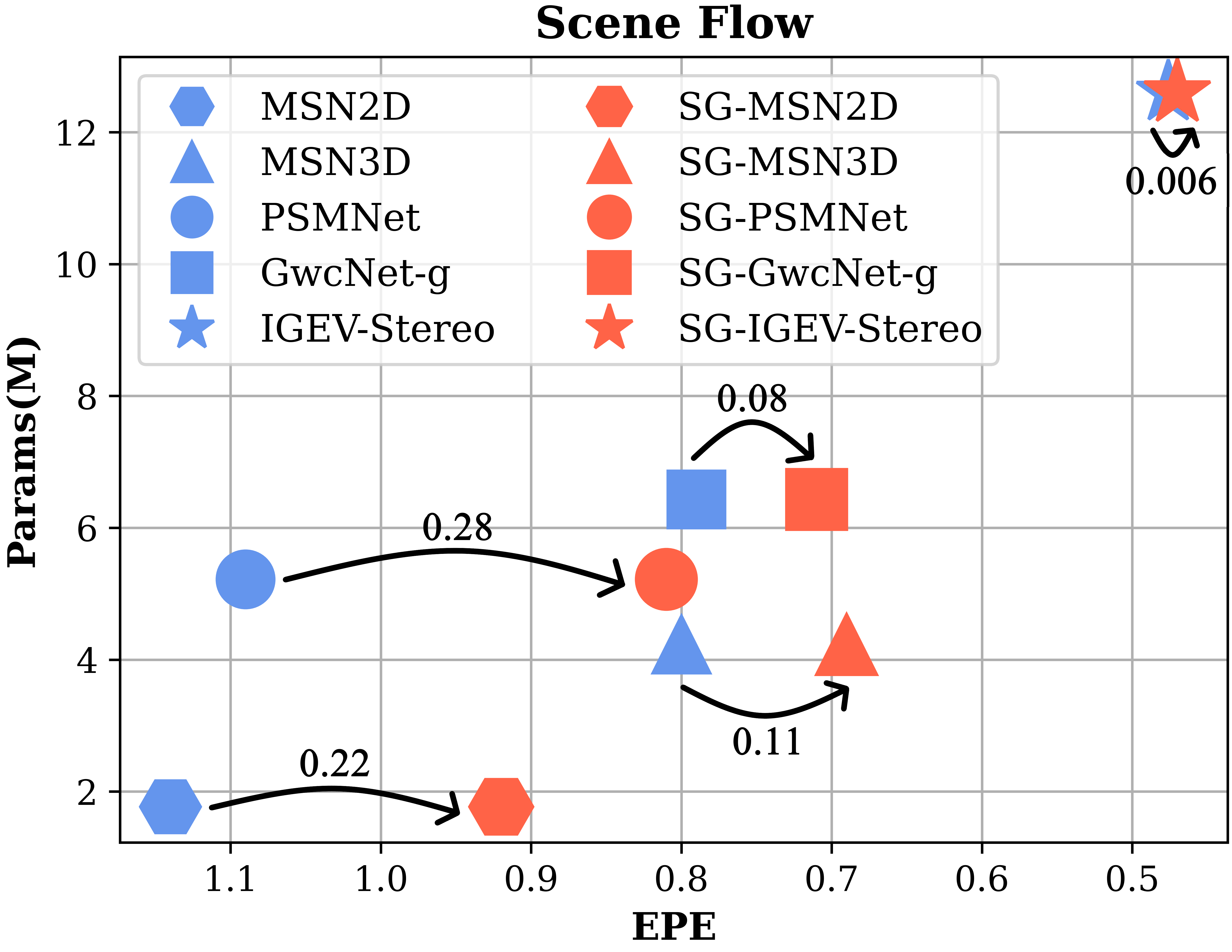
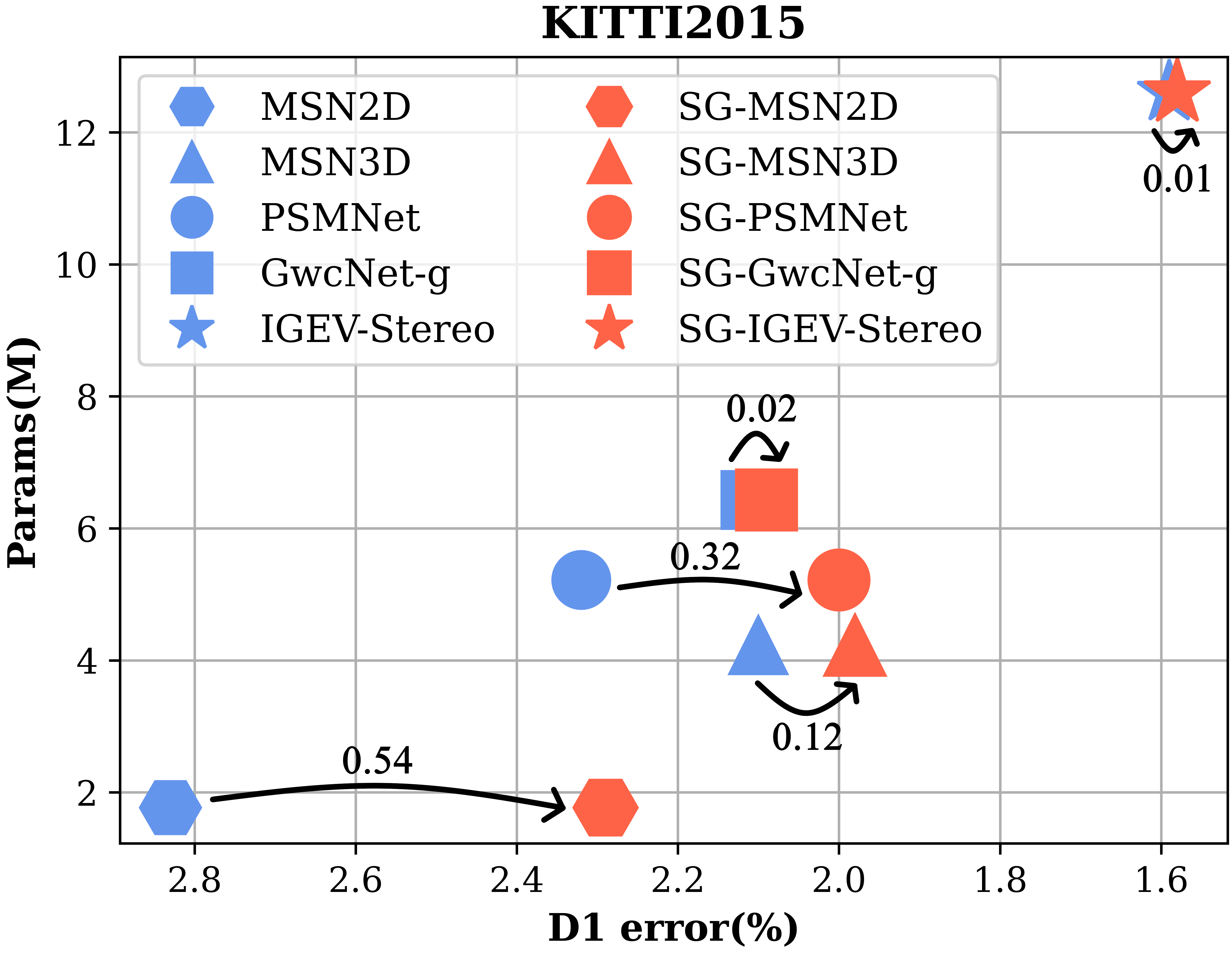
Figure 1: Quantitative comparisons on Sceneflow and Kitti. We implement our Sampling-Gaussian (SG) with five baseline methods for comparison. They are MSN2D and MSN3D (Shamsafar et al., 2021), PSMnet(Chang & Chen, 2018), GwcNet-g(Guo et al., 2019), IGEV-Stereo(Xu et al., 2023)

Stereo matching is a fundamental topic of computer vision which has been a subject of extensive research for many years. Accurate stereo matching is essential for deriving scene depth through the triangulation by the displacement of corresponding points in binocular images. The applications of stereo matching cover a wide range of advanced technologies, including autonomous driving, robot navigation, and drone control.

The common baseline of end-to-end learning-based stereo matching (Mayer et al., 2016b) comprises three key modules: feature extraction, cost volume aggregation, and soft-argmax-based disparity regression (Kendall et al., 2017). Features are extracted from the input image pair via a siamese network architecture. Subsequently, a 5D ($B,C,D,H,W$) cost volume is generated by concatenating features from the left and right images, while the disparity is the extra dimension $D$. This cost volume then serves as input to a disparity regression module, which employs 3D convolutions to refine the output. Kendall et al. (2017) was the first to leverage soft-argmax to achieve differentiable regression of disparity. Its efficiency and simplicity have made it a popular baseline for numerous subsequent studies (Chang & Chen, 2018; Pan et al., 2020; Wang et al., 2021; Xu et al., 2022; Shen et al., 2023). In the pursuit of accuracy, various innovative modules have been proposed for improvement, feature fusion(Xu & Zhang, 2020; Guo et al., 2019), robust aggregation(Zhang et al., 2019a; Shamsafar et al., 2021), iterative regression(Teed & Deng, 2021; Xu et al., 2023; 2024a). Nevertheless, soft-argmax remains a key component of these methods.

As the cost volume went through 3D CNNs, the channel is progressively reduced to 1. Then soft-argmax (Equ. 1) module is applied to obtain the disparity.

$$d=\sum_{i}i*softmax(z_{i})=\sum_{i}i*\frac{e^{z_{i}}}{\sum e^{z_{i}}}.$$ (1)

$d$ denotes the averaged disparity. $i$ and $softmax(z_{i})$ denotes the index of disparity and the probability of $i$.

$$smoothl1(d,\hat{d})=\left\{\begin{matrix}0.5(d-\hat{d})^{2},&if|d-\hat{d}|<1\\ |d-\hat{d}|-0.5,&otherwise\end{matrix}\right.,$$ (2)

Then a smoothl1 loss (Equ. 2) is used to measure the distance between $d$ and ground-truth $\hat{d}$. As soft-argmax is widely adopted, researchers have also noticed its limitations. Kendall et al. (2017) regarded the soft-argmax as a probability distribution of disparity and point out it’s prone to being influenced by multimodal distribution as it estimates a weighted summation of all modes. Similarly, Chen et al. (2019) demonstrated that the averaged disparity of multimodal is deviated from the center of the dominating mode. They conclude that the ambiguous matching is the cause of multimodal problem. Researchers have proposed various methods that aimed to solve the problem (Häger et al., 2021; Bangunharcana et al., 2021; Tulyakov et al., 2018; Xu et al., 2024b). Those methods can be broadly summarized as two steps, constructing a direct supervision signal for the probability distributions to be predominately unimodal, and limiting the disparity range of soft-argmax through a post-processing.

It’s challenge to reduce the ambiguous matching relies on network’s regularization only. Therefore, Tulyakov et al. (2018) taken the ground-truth disparity as the center $\mu$ of a discrete Laplacian distribution,

$$q(x)=\frac{1}{2b}e^{\frac{-|x-\mu|}{b}},$$ (3)

where $q(x)$ is the probability of integer $x$. And they optimize the network with cross-entropy loss,

$$H(p,q)=\sum_{x\in[d_{min},d_{max})}p(x)log(q(x)),$$ (4)

$p$ is the estimated probability. Following their ideas, different distribution are adopted, Gaussian(Chen et al., 2019), Laplacian(Tulyakov et al., 2018; Xu et al., 2024b; Liu et al., 2021; Zhang et al., 2019b) and Dirac impulse Häger et al. (2021), etc. This first step will effectively force the network learns to estimate a distribution that centered at the highest likelihood. To further mitigate the effects of full-band weighted summation, most of the methods proposed limiting the disparity range of the summation to the neighbors of the highest likelihood. Those methods have two issues. Firstly, the network trained with cross-entropy tends to locate the highest likelihood. However, due to the absence of explicit constraints, the values of each distribution are imprecise, resulting in a deviated disparity. The second step is implemented through Top-k or equivalent operation. But consequently results in an efficiency reduction due to the operation is not parallelizable.

To address those problems, we propose a novel Gaussian distribution-based supervision method with combined loss for stereo matching called Sampling-Gaussian. As shown in Fig. 1, our method achieves notable improvement over the listed commonly used baselines. Additionally, our method does not rely on Top-k or any other post-processing. Our method can be directly applied to any soft-argmax-based stereo matching algorithms without a decrease in efficiency. In section 3, we conduct a theoretical analysis of soft-argmax to fundamentally explain the reason of distribution-based supervision outperforms single value-based supervision. Moreover, we explore why previous methods have failed to improve the accuracy directly and concluded two reasons. First is the settings of the minimum and maximum disparity, which was empirically set to $0$ and $192$. Consequently, the regression near the endpoints are overlooked. Second is the trilinear interpolation which was used to upsample the cost volumes. The upsampled possibility distribution is impossible to fit the target distribution. We have conducted comprehensive ablation studies to illustrate the necessity of our proposed modules. Furthermore, we have implemented our method with five popular baselines(Chang & Chen, 2018; Shamsafar et al., 2021; Guo et al., 2019; Xu et al., 2023) to demonstrate that our method is easy to implement and universally applicable. At last, our method has also achieved state-of-the-arts results on Sceneflow(Mayer et al., 2016a) and Kitti2012, (Geiger et al., 2012), Kitti2015(Menze & Geiger, 2015).

In conclusion, our contributions has three folds:

• Our proposed Sampling-Gaussian can effectively improve the accuracy of stereo matching method. Moreover, we provide a new view by our interpretation of the distribution-based training.

• We have identified the two fundamental reasons that lead to the inferior performance of distribution-based methods. Moreover, we provide theoretical explanations and solutions.

• We conducted comprehensive experiments to demonstrate that Sampling-Gaussian can be implemented to various methods and achieves notable improvement. Our method is easy to implement and code is open-sourced.

2 Related Works

2.1 The baseline of stereo matching

Stereo matching method is a method that calculates the disparity map of the binocular images with size $(H,W)$. The feature network(Kendall et al., 2017; He et al., 2015) extracts the features with size $(\frac{H}{4},\frac{W}{4})$. Then the cost volume is constructed with size $(\frac{d_{max}}{4},\frac{H}{4},\frac{W}{4})$, where $d_{max}$ is a hyperparameter and empirical set to 192(Chang & Chen, 2018). A disparity regression network with 3D convolutions is used for refine the cost volume. Its output remains the same size as cost volume. Then a trilinear interpolation operation is used for upsample the output to $(d_{max},H,W)$. At last, a soft-argmax operation is applied.

2.2 Improvement methods

Based on the baseline, the subsequent proposed improvement methods can be classified into several levels: feature level, module level, baseline level, and distribution level. Firstly, at the feature level, Chang & Chen (2018) proposed the PSMNet which adopts a spatial feature pyramid(He et al., 2014) to extract and fuse multi-resolution features, and stacked-hourglass module is adopted as regression module to improve the refinement. Based on PSMNet, Guo et al. (2019) proposed a group-wise correlation network(GwcNet) which calculates the dot products of the left and right features instead of a concatenation. And at module level, Zhang et al. (2019a) proposed a guided-aggregation module to better refine the cost volume. And Xu et al. (2022) leverages attention mechanism to supervise the cost volume. At the baseline level, researchers proposed new baselines to improve the accuracy of the efficiency. Xu & Zhang (2020) and Pan et al. (2020) proposed to progressively aggregate the cost volume to the full size. Others proposed 2DConv-based methods(Pan et al., 2024; Shamsafar et al., 2021) to reduce the high FLOPs. And Xu et al. (2023) proposed to iterative refine the disparity and significantly improve the accuracy but at the expense of speed.

2.3 Distribution-based improvement method

The soft-argmax operation is widely applied in various tasks as it retrieves the index of the highest probability in a differentiable way. Despite its efficiency, researchers continuously explore and propose better methods. From a distribution-view, the soft-argmax is equivalent to retrieves the mean of the probability distribution(Li et al., 2021). Consequently, network trained with soft-argmax lacks explicit supervision for the distribution, resulting in unconstrained probability shape.

However, this disadvantage of soft-argmax receives less attention than other aspect. Because, as the network become deeper and larger, the multimodal problem can be solved partially by the network’s generalization ability. The DSNT (Nibali et al., 2018) introduced a differentiable operation to render the heatmap with a 2D Gaussian kernel as a constraint for shape. Some methods attribute inaccurate estimates to the multimodal problem. The PDS (Tulyakov et al., 2018) limit the range of the soft-argmax with Top-k during inference in order to solve the multimodal problem. An unresolved issue with PDS is its lack of robustness, as the range parameter is set in advance. A corresponding solution was proposed in Liu & Liu (2022), using learned weights to suppress unreliable disparity regions. A similar idea was proposed in Häger et al. (2021), where they use a Dirac impulse to model the distributions.

3 Explorations

In this section, we first analyze the biased gradient of soft-argmax to establish that distribution-based supervision is necessary for stereo matching. Then, we analyze the two basic settings that have led previous distribution-based methods to their inferior improvements.

3.1 Analysis of biased gradient

We first analysis the partial differential equation of soft-argmax. The $e^{z_{i}}$ denotes the input of softmax. The partial derivative of $e^{z_{i}}$ is defined as

$$\frac{\partial L}{\partial e^{z_{i}}} =\frac{\partial L}{\partial d}\frac{\partial d}{\partial e^{z_{i}}}$$ (5)

$$=\frac{\partial L}{\partial d}(i\frac{e^{z_{i}}}{\sum e^{*}}(1-\frac{e^{z_{i}}}{\sum e^{*}})+\sum_{j\neq i}j(-\frac{e^{z_{j}}}{\sum e^{*}}*\frac{e^{z_{i}}}{\sum e^{*}}))$$

$$=\frac{\partial L}{\partial d}(\frac{e^{z_{i}}}{\sum e^{*}}({i}-d)).$$

The variable $i$ denotes the corresponding index, and $d$ denotes the result of Equation 1. It is evident that $i$ would always receive a weight $(i-d)$ to the gradient that is proportional to its distance to $d$. Therefore, it is difficult for the network to reach the global minimum since the gradient is biased.

3.2 Analysis of distribution-based method

Two basic settings are widely adopted, the disparity range $[0,192)$, and trilinear interpolation.

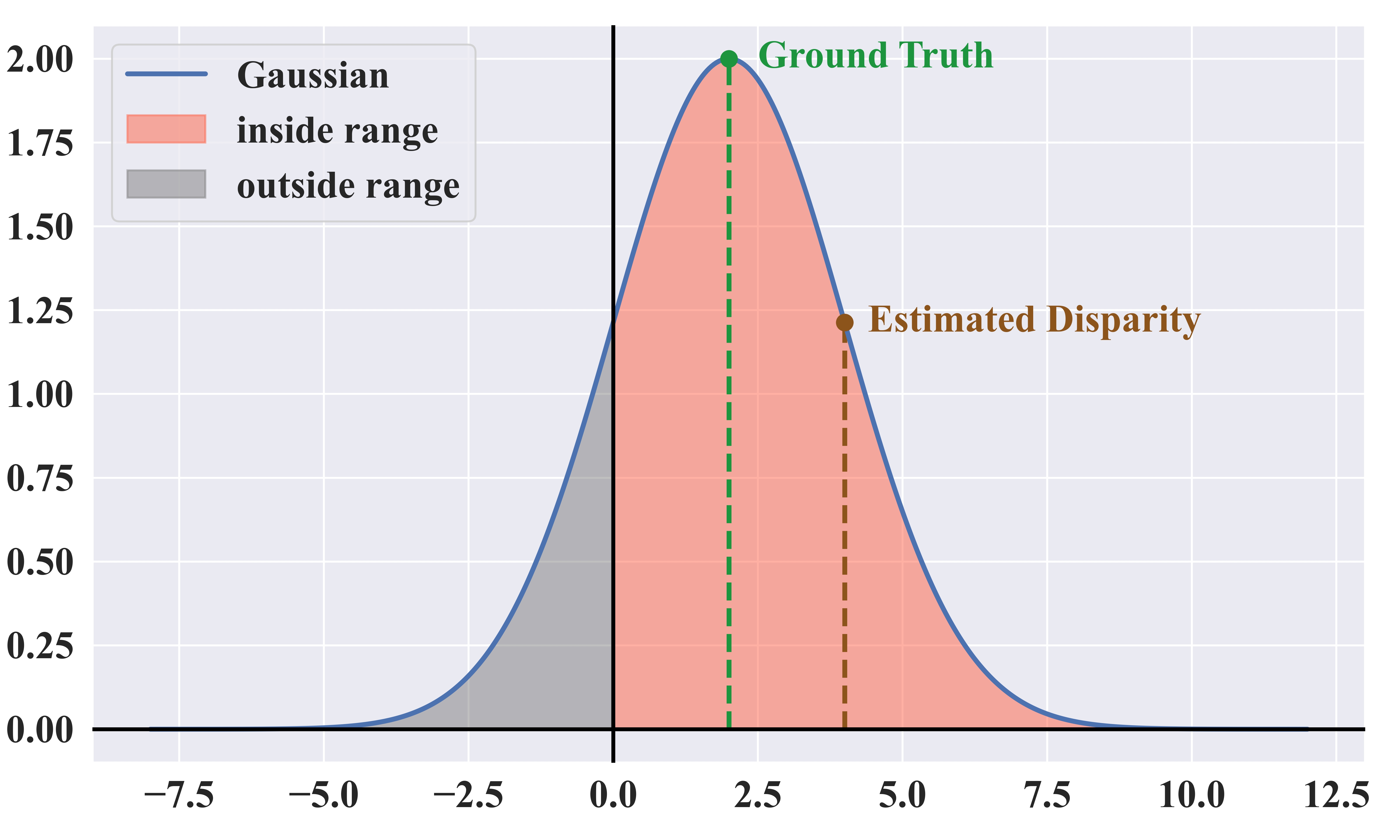
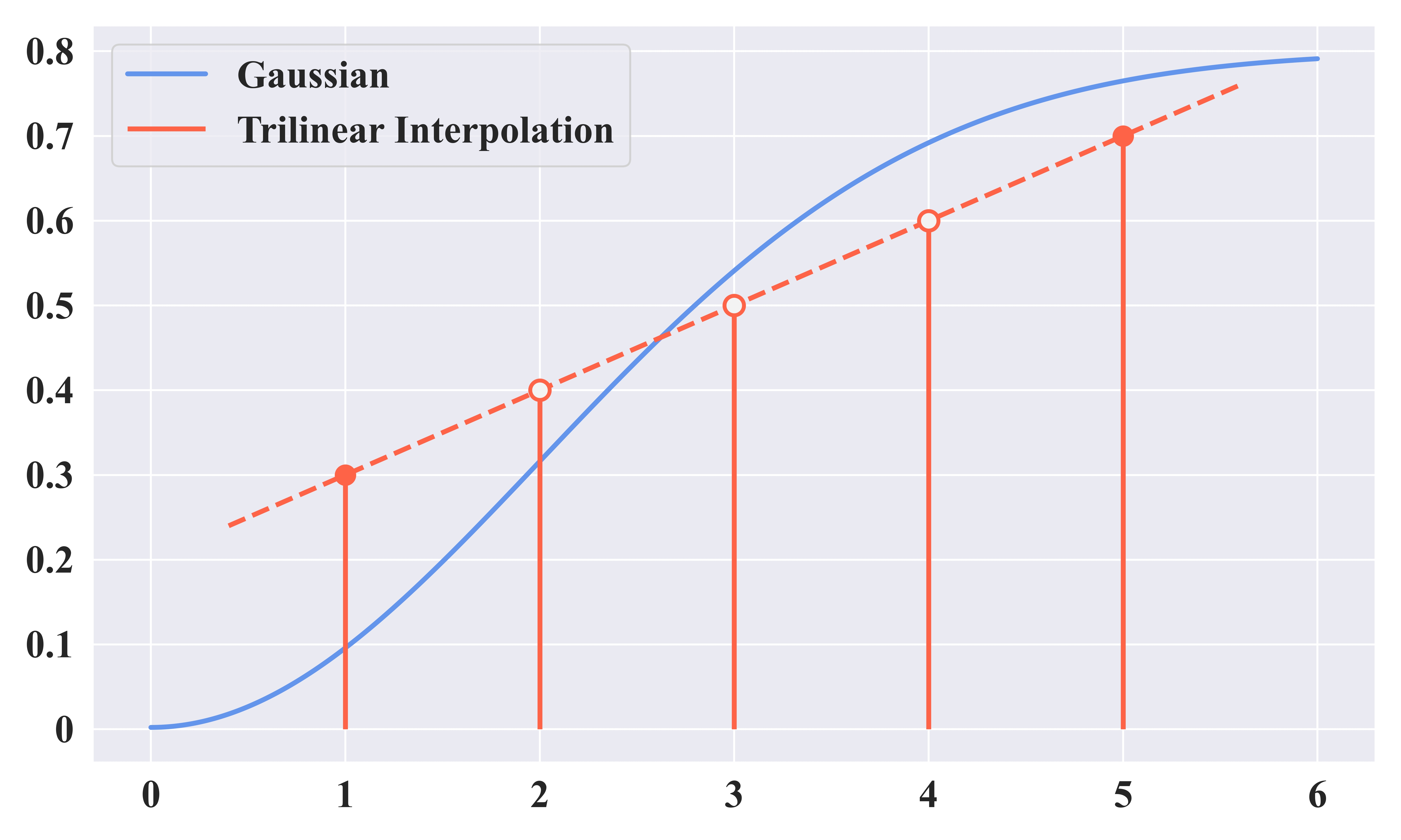
Figure 2: The left plot shows the impact of the disparity range. The predicted disparity near the endpoints is deviated. The right plot shows that after trilinear interpolation, the probabilities are linearly distributed and are unable to fit the Gaussian distribution.

a) This setting of range is inherited from the soft-argmax-based method. However, for distribution-based method, it would lead to a deviated disparity. For instance, a distribution $q$ is sampled based on Equ (3) when ground-truth equals $0$. And the expectation of q, which is equivalent to calculates the soft-argmax, is $0$ when the range is infinite.

$$\sum_{x=-\infty}^{\infty}x*q(x)=0<\sum_{x=0}^{\infty}x*q(x).$$ (6)

And if the minimum disparity is set to $0$, the expectation of q would be deviated. It’s same for the maximum disparity.

b) After the trilinear interpolation, the cost volume is linearly resized from $\frac{d_{max}}{4}$ to $d_{max}$. However, whether the Laplacian or Gaussian distribution are taken for the supervision, their distribution is convex. As a result, it is impossible for the network to converge.

4 The proposed Sampling-Gaussian

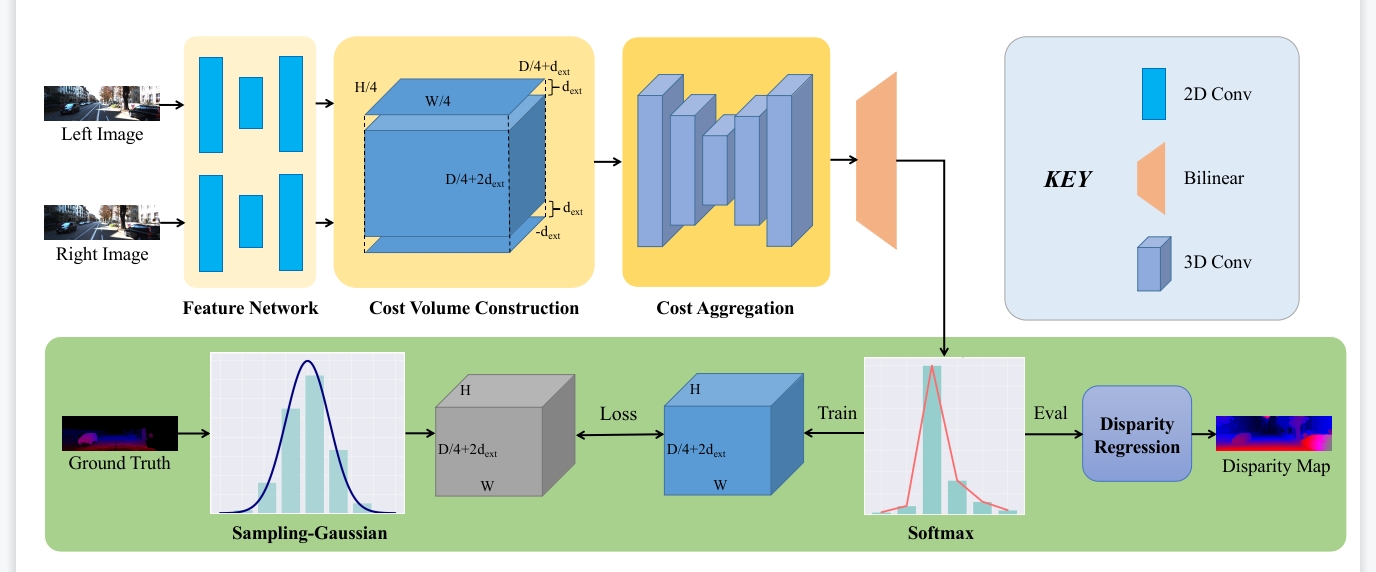
Figure 3: The workflow of our proposed Sampling-Gaussian

In this paper, we present an innovative interpretation of the soft-argmax and distribution-based supervision from the perspective of vector space. Therefore, the training process can be regarded as minimizing the distance between two vectors. Based on this interpretation, we propose the Sampling-Gaussian, which consists of three parts.

4.1 Construct the distribution

First, we leveraged the probability density function of Gaussian distribution to sample the discrete supervision signal within an extended disparity range. The original disparity range is $[0,d_{max})$, we extend the range to $D=[-d_{ext},d_{max}+d_{ext})$, the size of D$=d_{max}+2*d_{ext}$. The sampling function is defined as

$$q(x)=\frac{e^{-\frac{(x-\mu)^{2}}{2\sigma^{2}}}}{\sum_{x}e^{-\frac{(x-\mu)^{2}x-\mu}{2\sigma^{2}}}}.$$ (7)

The $\mu$ is the ground-truth disparity. $\sigma$ is used to control the shape, and $0.5$ achieves the best result.

4.2 Structure alterations

As we extended the disparity range by $d_{ext}$, the size of cost volume $C$ is also changed. The construction of $C$ involves iteratively constructing the $C$ by shifting the feature map by $1$ pixel,

$$C(c,d,x,y)=g(f_{l}(.,x,y),f_{y}(.,x-d,y)).$$ (8)

The $f_{l},f_{r}$ denotes the features of left and right image. And $g$ denotes a fusion method for features, usually is group-wise correlation(Guo et al., 2019) or concatenation(Chang & Chen, 2018). And the size of $C$ is $[B,C,\frac{D}{4},\frac{H}{4},\frac{W}{4}]$.

Then, a bilinear interpolation is leveraged to upsample the cost volume after the regression modules,

$$\textbf{C}=bilinear(C).$$ (9)

And the size of C is $[B,C,\frac{D}{4},H,W]$.

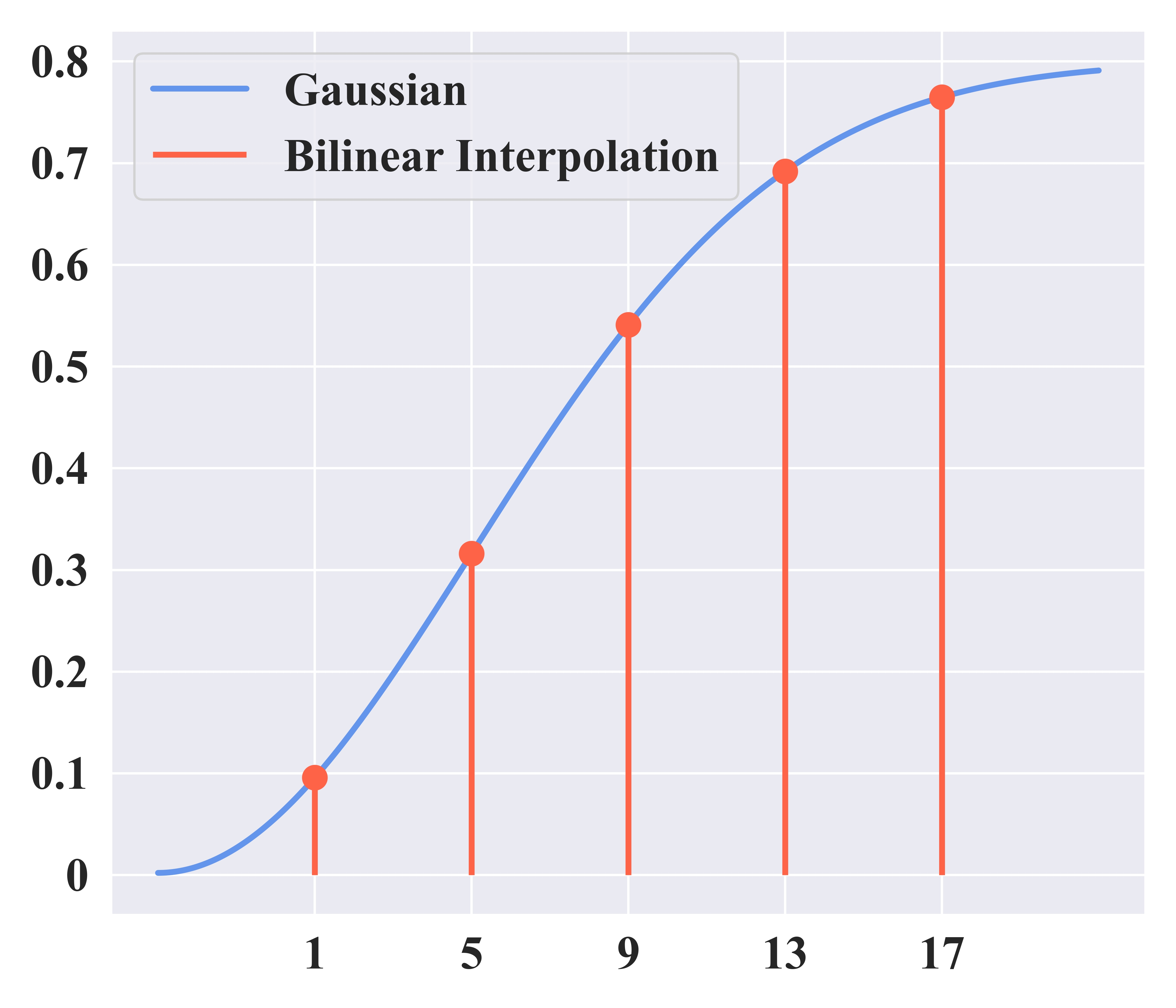
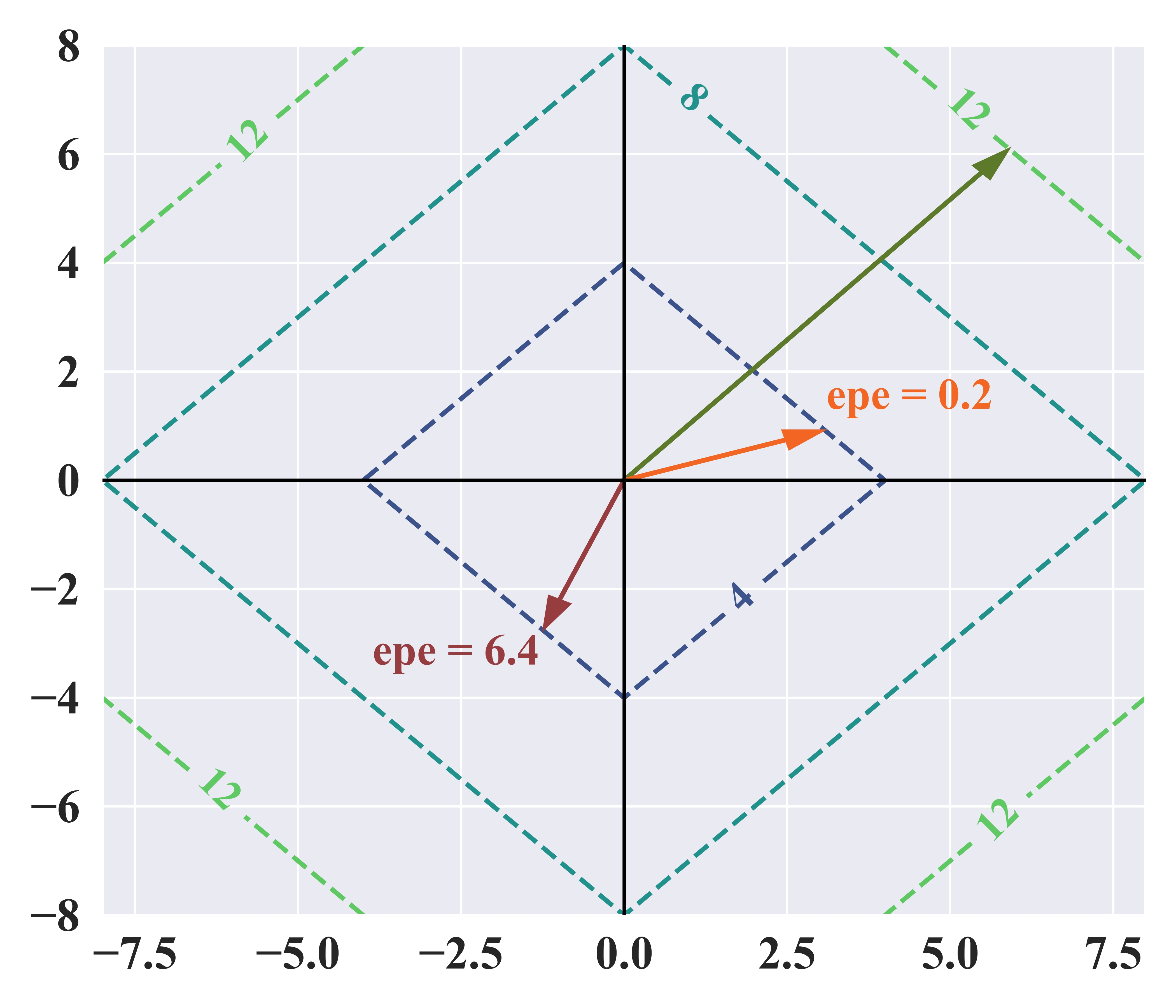
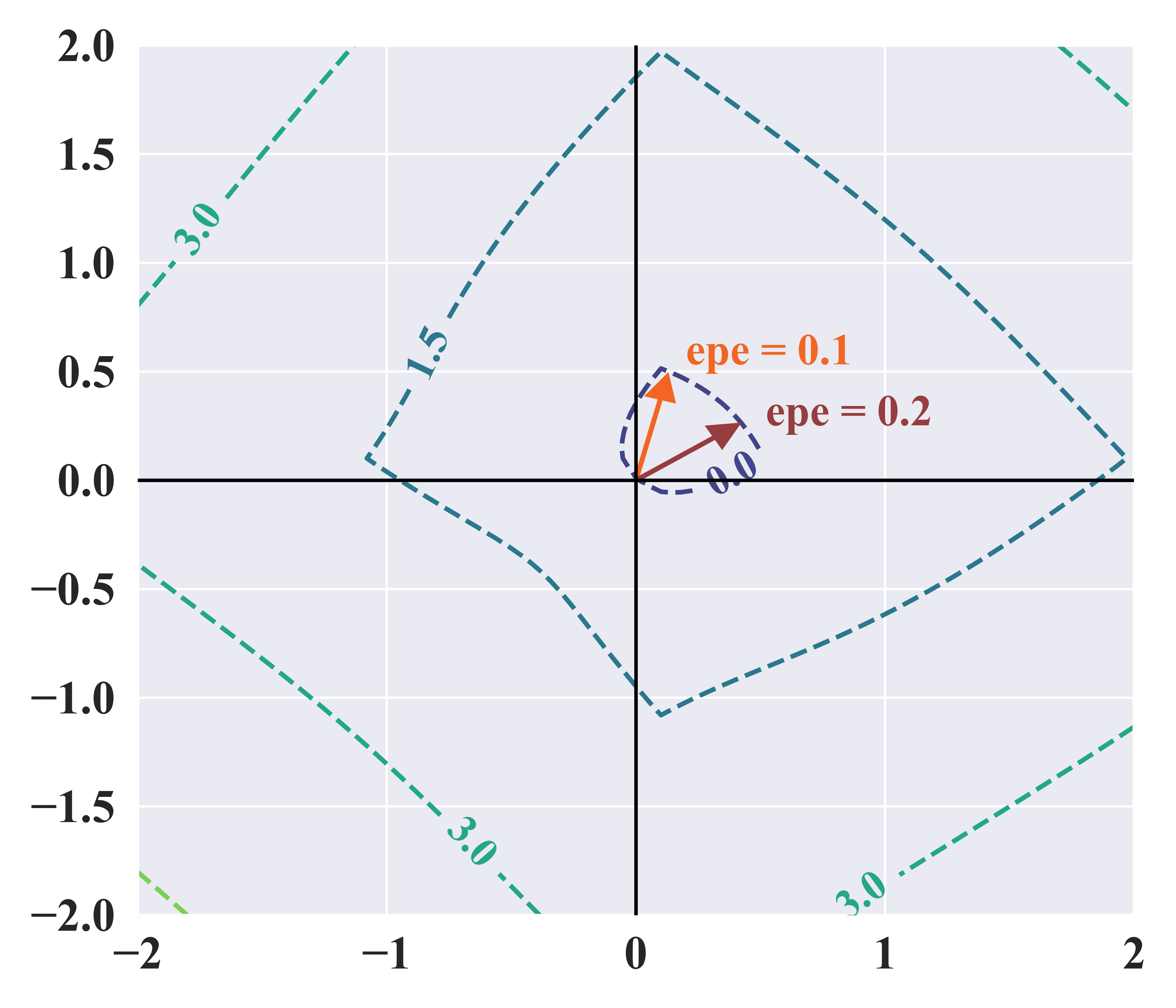
Figure 4: The left plot: Since the probabilities are not linearly related, therefore it can fit into the Gaussian distribution. The middle plot: The loss landscape of L1 loss, dashed lines are contour line. Two vectors with the same L1 loss, could result in significant difference in EPE. The right plot: The loss landscape of the combined loss and the EPE of two vectors with the same loss are similar.

4.3 Combination loss

The supervision distribution is $q$. The output of network is distribution $p=softmax(\textbf{C})$. The cross-entropy(Tulyakov et al., 2018; Chen et al., 2019; Xu et al., 2024b) loss can constrain the majority parts of the distribution but failed to optimize the distribution to further to exact value. As we interpret $p$ and $q$ as two vectors, we leverage L1 loss to measure the distance,

$$L_{1}(p,q)=\frac{1}{n}\sum_{i}^{n}|p(i)-q(i)|,$$ (10)

L1 loss is sensitive to all difference of value regardless of the index. However, this is also the disadvantage. As depicted in Fig. 4, that two vectors with same L1 loss to $q$, their predicted disparity could be very different.

In repose, we have proposed a negative cosine similarity to measure the difference in direction between $p$ and $q$,

$$L_{cos}(p,q)=-\frac{\sum_{i}^{n}p(i)q(i)}{\sqrt{\sum p(*)^{2}}\sqrt{\sum q(*)^{2}}}.$$ (11)

Then the two losses is combined with a weight $\lambda=0.5$,

$$L(p,q)=L_{1}(p,q)+\lambda*L_{cos}(p,q).$$ (12)

As shown in Fig. 4, the vectors on the same contour line has similar end-point error(EPE).

4.4 Inference

A key contribution of our method, is that we do not rely on Top-k operation for refinement. During the inference, we calculate the expectation of $p$ directly,

$$d=4*\sum i*p=4*\sum_{D/4}i*softmax(\textbf{C}_{i}),$$ (13)

which has the same form of soft-argmax. Therefore, our method can be easily implemented with most of the soft-argmax-based method. After the upsampling, the dimension of disparity remains one-fourth of original. Consequently, the value after regression is also one-fourth of the original. Thus, the “$4*$” is to recover the disparity to its original scale.

5 Experimental results

In this section, we report our implementation details and experimental results. We have implemented Sampling-Gaussian with $5$ most representative methods for comparisons:

1. PSMNet(Chang & Chen, 2018). The “ResNet” of the stereo matching. They outperformed SOTA algorithm by $5\%$ at the time. Their method is open-source, easy to read and replicate. We use this method for a wider range of comparisons.

2. GwcNet-g(Guo et al., 2019). A group-wise correlation module is proposed based on PSMNet. Their module is widely adopted. Code is open-sourced.

3$\&$4. MSN3D and MSN2D (Shamsafar et al., 2021): They have proposed lightweight networks by leveraging 2D convolutions to reduce computational expenses while maintaining accuracy.

5. IGEV-Stereo(Xu et al., 2023): Based on RAFT(Teed & Deng, 2021), they proposed an iterative refine module and achieves SOTA results. We implement our method with IGEV-stereo to demonstrates our methods is compatible with a variety of structure.

We conducted experiments mainly on two datasets: Sceneflow(Mayer et al., 2016b) is a large scale of synthetic stereo dataset which contains more than 35k training pairs and 4.3k testing pairs with resolution 960x540. Kitti(Geiger et al., 2012; Menze & Geiger, 2015) We use Kitti2012 and Kitti2015 for train and test. They contain 395 pairs for training and 395 pairs for testing in total, with resolution $1242\times 375$.

5.1 Implementation details

For simplicity, we will refer to our Sampling-Gaussian as SG. Our implemented versions of method are denoted as SG-PSMNet or SG-MS2D. Our method is implemented using the PyTorch framework. We conducted all the experiments on two A100 GPUs. We leverage AdamW(Loshchilov & Hutter, 2017) with $\beta_{1}=0.9,\beta_{2}=0.999$, weight decay$=10^{-2}$, as optimizer. All the networks are trained with similar protocol: train on Sceneflow for $20$ epochs with learning rate$=10^{-3}$. Then, finetuning on Kitti for $200$ epochs with lr$=10^{-3}$, then with lr$=10^{-4}$ for another $300$ epochs, and with lr$=10^{-5}$ for the last $300$ epochs. For IGEV-stereo and MSN2D, the parameters are slightly changed. Two metrics are adopted for evaluation (both are lower the better): End-point error (EPE)(Mayer et al., 2016b), commonly used in optical flow. It calculates the l1 loss. D1 error (Menze & Geiger, 2015) calculates the percentage of error pixels. Pixels with EPE larger than 3 will be considered as error.

5.2 Ablation studies

5.2.1 Sigma $\sigma$ of the Sampling-Gaussian

The $\sigma$ controls the shape of the distribution and directly affects the distribution pattern finally learned by the network. In table 1, we have conducted experiments to determine the influence of sigma on the model results.

Table 1: Quantitative comparisons on settings of $\sigma$

$\sigma$	$0.3$	$0.4$	0.5	$0.6$	$0.7$	$1.0$
PSMnet	$2.526$	$2.526$	0.625	$0.631$	$0.723$	$0.688$

When the $\sigma$ is set to $0.3$ or $1$, the shape of distribution is either too narrow or too wide. When the distribution is too narrow, higher requirements are imposed on the model’s predicted probability, which would lead to larger errors. If the $\sigma$ is too large, the targets becomes easier for the model to converge, but failed to further improve due to more values affect the final output.

Table 2: Quantitative comparisons on settings of $\sigma$.

Base	Trilinear	Bilinear	Loss	$\lambda$	EPE	D1
MSN2D	✓		L1	/	0.99	2.62
		✓	L1+Cos	0.5	0.91	2.49
PSMNet	✓		CE	/	0.94	2.34
	✓		L1	/	0.87	2.15
	✓		L1+Cos	0.5	0.89	2.26
		✓	L1+Cos	0.2	0.79	2.15
		✓	L1+Cos	1.0	1.23	2.86
		✓	L1+Cos	0.5	0.65	2.00

5.2.2 Interpolation method

To demonstrate the effectiveness of the proposed bilinear interpolation, we have conducted experiments to compare bilinear interpolation with trilinear interpolation. As shown in table 2, bilinear interpolation has achieved better results with two methods, which aligns with our theory.

5.2.3 Losses and Lambda $\lambda$

We have also conducted experiments to compare the performance of different combination of losses and weight $\lambda$. As shown in table 2, even though the cross-entropy(CE) loss has achieved only $0.94$, the network converges faster than trained with L1 loss. Regarding the combination of L1 and Cosine similarity(Cos), if the $\lambda$ is too large, the network would eventually collapse.

5.2.4 Extended range

At last, we conducted comparisons between with or without the extended range of disparity. As table 3 shown, it has a positive effect on the performance.

Table 3: Ablation study on disparity range

$d_{ext}$	EPE	$<1$	$<3$
0	0.69	6.72	2.32
16	0.65	5.31	2.00

5.3 Quantitative comparisons

Table 4: Quantitative comparison on Sceneflow

Method	EPE	D1	Params	Supervision	Loss	Top-k	Time(s)
PDS	1.12	2.93	2.2	Combined*	CE	Y	/
MSN2D	1.14	2.83	2.23	Soft-argmax	Smoothl1	N	0.10
PSMNet	1.09	2.32	5.22	Soft-argmax	Smoothl1	N	0.41
PSMNet+	1.02	3.12	2.32	Laplacian	CE	Y	/
Acfnet	0.87	4.31	/	Combined*	CE+Focal	N	0.48
MSN3D	0.80	2.10	1.77	Soft-argmax	Smoothl1	N	0.53
GwcNet-g	0.79	2.11	6.43	Soft-argmax	Smoothl1	N	0.32
GANet+LaC	0.72	6.52	9.43	Combined*	L1+CE	Y	1.72
GANet+ADL	0.50	1.81	9.43	Laplacian	L1+CE	Y	1.72
IGEV-Stereo	0.47	1.59	12.60	Soft-argmax	L1	N	0.37
SG-MSN2D	0.91	2.49	2.23	Gaussian	L1+Cos	N	0.10
SG-PSMNet	0.65	2.00	5.22	Gaussian	L1+Cos	N	0.41
SG-GwcNet-g	0.71	2.09	6.43	Gaussian	L1+Cos	N	0.32
SG-MSN3D	0.69	1.98	1.77	Gaussian	L1+Cos	N	0.53
SG-IGEV-Stereo	0.47	1.58	12.60	Gaussian	L1+Cos	N	0.37
Combined*: combination of Soft-argmax and Laplacian

In this section, we compared with the SOTA methods and most relative methods on Sceneflow Mayer et al. (2016b), Kitti2012(Geiger et al., 2012) and Kitti2015(Menze & Geiger, 2015). In table 4, we compared with PDS(Tulyakov et al., 2018), Acfnet(Zhang et al., 2019b),PSMNet+(Chang & Chen, 2018), GANet+LaC(Liu et al., 2021), GANet+ADL(Xu et al., 2024b). As shown, most methods utilize Top-k or other post-processing modules or integrate soft-argmax for supervised training. These methods employ additional modules, which leads to an increase in latency. In contrast, our method effectively improves the accuracy of the baseline and keeps the architecture unchanged, thus ensuring consistent and efficient inference.

Table 5: The quantitative comparison on Kitti2012 and Kitti2015, the evaluation metrics are d1, $<2$ and $<3$ error rate($\%$). All are lower the better.

	Kitti2015-All			Kitti2015-Noc			Kitti2012
Method	$d1_{bg}$	$d1_{fg}$	$d1_{all}$	$d1_{bg}$	$d1_{fg}$	$d1_{all}$	$<2$	$<3$
MSN2d(Shamsafar et al., 2021)	2.49	4.53	2.83	2.29	3.81	2.54	$\backslash$	$\backslash$
PDSNetTulyakov et al. (2018)	2.29	4.05	2.58	2.09	3.68	2.36	4.65	2.53
PSMnet(Chang & Chen, 2018)	1.86	4.62	2.32	1.71	4.31	2.14	3.01	1.89
PSMnet+CE(Chen et al., 2019)	1.54	4.33	2.14	1.70	3.90	1.93	2.81	1.81
GwcNet-g(Guo et al., 2019)	1.74	3.93	2.11	1.61	3.49	1.92	$\backslash$	$\backslash$
MSN3d(Shamsafar et al., 2021)	1.75	3.87	2.10	1.61	3.50	1.92	$\backslash$	$\backslash$
AAnet+(Xu & Zhang, 2020)	1.65	3.96	2.03	1.49	3.66	1.85	2.96	2.04
RAFT(Teed & Deng, 2021)	1.48	3.46	1.81	1.34	3.11	1.63	$\backslash$	$\backslash$
GANetZhang et al. (2019a)	1.48	3.46	1.81	1.34	3.11	1.63	2.50	1.60
ACVNet(Xu et al., 2022)	1.37	3.07	1.65	1.26	2.84	1.52	2.34	1.47
RT-IGEV++ (Xu et al., 2024a)	1.48	3.37	1.79	1.34	3.17	1.64	2.51	1.68
PSMNet+ADL(Xu et al., 2024b)	1.44	3.25	1.74	1.30	3.04	1.59	2.17	1.42
LEAstereoCheng et al. (2020)	1.40	2.91	1.65	1.29	2.65	1.51	2.39	1.45
IGEV-stereo(Xu et al., 2023)	1.38	2.67	1.59	1.27	2.62	1.49	2.17	1.44
SG-MSN2d	1.94	4.07	2.29	1.78	3.63	2.08	3.15	2.09
SG-GwcNet-g	1.73	3.88	2.09	1.59	3.55	1.92	2.89	1.95
SG-PSMnet	1.77	3.13	2.00	1.65	2.97	1.87	2.69	1.80
SG-MSN3d	1.61	3.81	1.98	1.48	3.55	1.82	2.62	1.74
SG-IGEV-stereo	1.40	2.50	1.58	1.30	2.48	1.50	2.12	1.39

The comparisons on Kitti are listed in table 5. As shown, our approach can effectively improve the results of all baselines. As the results indicate, the smaller the model, the greater the improvement. On MSN2D, we have achieved improvement of 0.54%. And we also have obtained an improvement of 0.01% on IGEV-stereo and achieved state-of-the-art results. Hence, it can be concluded that our method can effectively improve the generalization ability of the model, regardless of the model size. The improvement is particularly prominent on models with poor generalization.

5.4 Qualitative comparisons

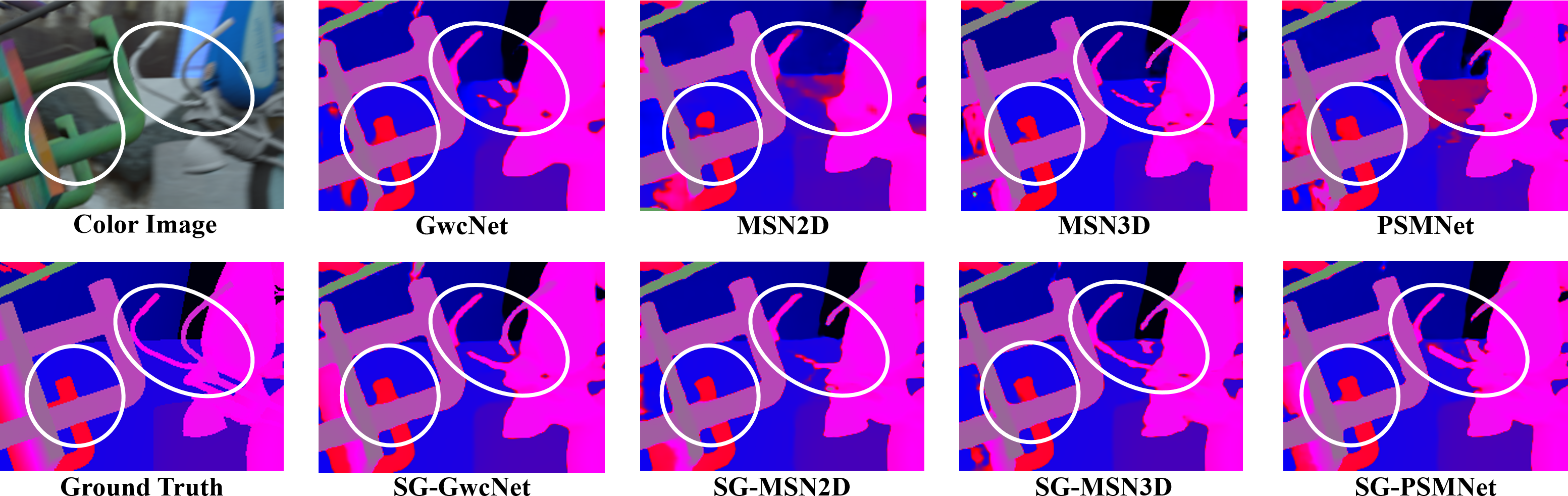
Figure 5: Qualitative comparisons on Sceneflow

Through experiments, we found that our Sampling-Gaussian effectively improves the accuracy of the model to predicts small objects and details, as depicted in Figure 5. The reason is that models trained with Soft-argmax are prone to converge to the majority of the disparity, while details are relatively in the minority. On the other hand, our SG provides explicit supervision for all objects. Therefore, the model gains the ability to capture details.

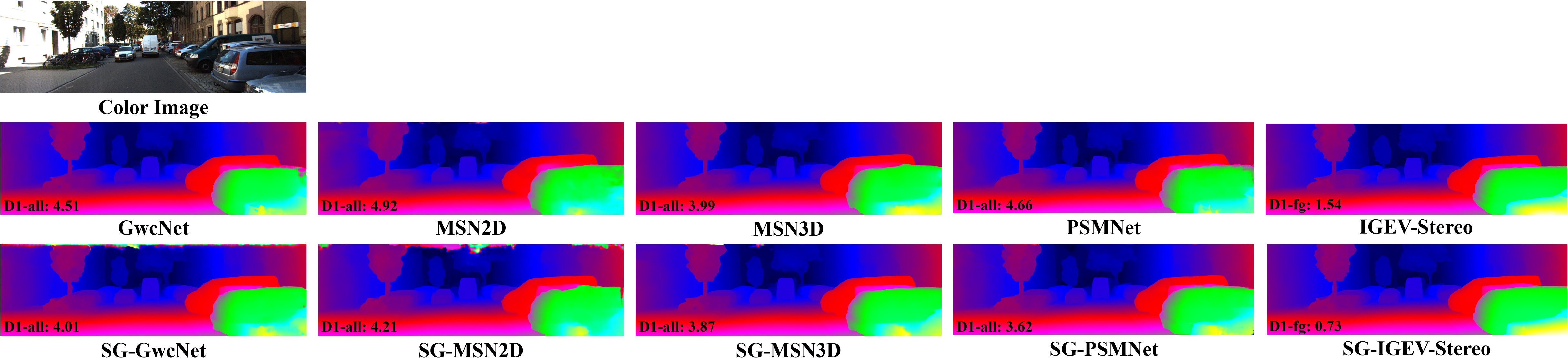
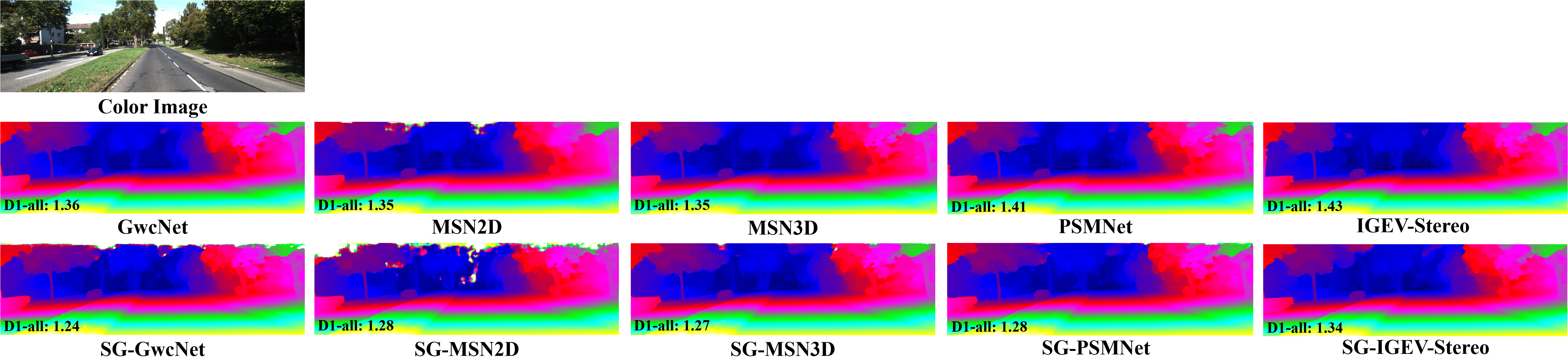
Figure 6: Qualitative comparisons on Kitti2015

In the first example in Fig. 6, it is evident that all baselines trained with SG have gained the ability to capture details to different degrees. For instance, in the disparity of the right side van and the shape of the trees in the background. More of our results are available on the Kitti2012 and Kitti2015 leaderboard.

5.5 Cross-domain generalization

At last, we have conducted experiments to compare the cross-domain generalization ability of our methods. We have trained baselines on Sceneflow, and evaluate on Kitti2015 directly. Our method has improved the generalization ability of the baselines. Qualitative results are available in appendix.

Table 6: Cross-domain generalization evaluation

	Kitti2015-ALL					Kitti2015-ALL
Base	EPE	$>1$	$>2$	$>3$	Ours	EPE	$>1$	$>2$	$>3$
MSN2D	5.03	56.1	33.7	24.4	SG-MSN2D	1.53	48.2	22.2	12.5
MSN3D	29.4	72.2	57.7	50.0	SG-MSN3D	22.5	53.7	26.3	17.3
PSMNet	21.1	88.6	64.7	48.8	SG-PSMNet	24.6	78.0	65.0	57.2

6 Conclusions

In this paper, we introduce a novel training method Sampling-Gaussian for stereo matching. We have solved the fundamental problems of previous distribution-based method by extend the disparity range and bilinear interpolation. Moreover, we interpret the learning process as minimizing the distance in the vector space, and proposed a combined loss. Through comprehensive comparisons with five baseline methods, we demonstrate that our Sampling-Gaussian achieves improvements through all the methods, and fulfill our goal in proposing an effective and easy to implement method. In the future, we are going to study the generalization ability of stereo matching networks in order to solve the applications in real-life.

Appendix A Appendix

A.1 Full equation of Equ. 5

The first part is the full equation of Equ 5.

$$\frac{\partial L}{\partial e^{z_{i}}} =\frac{\partial L}{\partial d}\frac{\partial d}{\partial e^{z_{i}}}$$ (14)

$$=\frac{\partial L}{\partial d}(i\frac{e^{z_{i}}}{\sum e^{*}}(1-\frac{e^{z_{i}}}{\sum e^{*}})+\sum_{j\neq i}j(-\frac{e^{z_{j}}}{\sum e^{*}}*\frac{e^{z_{i}}}{\sum e^{*}}))$$

$$=\frac{\partial L}{\partial d}(i\frac{e^{z_{i}}}{\sum e^{*}}+i(-\frac{e^{z_{i}}}{\sum e^{*}}*\frac{e^{z_{i}}}{\sum e^{*}})+\sum_{j\neq i}j(-\frac{e^{z_{j}}}{\sum e^{*}}*\frac{e^{z_{i}}}{\sum e^{*}}))$$

$$=\frac{\partial L}{\partial d}(i\frac{e^{z_{i}}}{\sum e^{*}}+\sum_{j}(-\frac{e^{z_{j}}}{\sum e^{*}}*\frac{e^{z_{i}}}{\sum e^{*}}))$$

$$=\frac{\partial L}{\partial d}(\frac{e^{z_{i}}}{\sum e^{*}}(i-\underline{\sum j*\frac{e^{z_{j}}}{\sum e^{*}}}))$$

$$=\frac{\partial L}{\partial d}(\frac{e^{z_{i}}}{\sum e^{*}}(i-d))$$

the part with underline is the equation of soft-argmax Equ. 1,

A.2 Python Implementation

This is the python implementation of Sampling-Gaussian.

A.3 Probabilities of Sampling-Gaussian

Table 7: The accuracy of the Sampling-Gaussian’s cumulative possibility and expectation.

$\mu$	$1-\sum_{x}p$	$\mu-\sum_{x}d*p$
4	$0.005296$	$-0.37134$
5	$0.004317$	$-0.02964$
6	$3.14e-05$	$-0.00178$
7	$1.10e-06$	$-6.2e-05$
8	$2.37e-08$	$-1.3e-06$
7	$1.10e-06$	$-6.2e-05$
8	$2.37e-08$	$-1.3e-06$
9	$3.07e-10$	$-1.8e-08$
10	$2.39e-12$	$-1.4e-10$
11	$1.09e-14$	$-6.8e-13$
12	$0.00$	$7.10e-15$
15	$0.00$	$0.00.0$
20	$0.00$	$7.10e-15$

Let’s review the equation 7. First, the probability density function of the discretized Gaussian distribution is defined as

$$q(x)=\frac{1}{\sigma*\sqrt{2\pi}}e^{-\frac{(x-\mu)^{2}}{2\sigma^{2}}}$$ (15)

The Riemann sum of the equation 15 is

$$\int_{a}^{b}e^{-\frac{(x-\mu)^{2}}{2\sigma^{2}}}dx\approx\frac{1}{2}(f(x_{0})+2f(x_{1})\dots+2f(x_{N-1})+f(x_{N}))$$ (16)

We further evaluate the summation of probability of Equ. 16. Thus, we need to evaluate the Sampling-Gaussian’s cumulative possibility. As shown in Table 7. The table shows, that the cumulative possibility is not strictly equals to $1$. However, the probabilities predicted by the network is strictly equals to $1$ due to the softmax operation. Therefore, in Equ. 7, the probabilities is divided by the summation of the probabilities. Thus, the summation is strictly equals to $1$.

The table 7 shown the range inside the $[0,d_{max})$. Which illustrate the reason of why $d_{ext}$ is needed. Moreover, as depicted in table 7. The cumulative possibility is not always equals to 1. Therefore, the division by the summation of the probabilities is an effective to strictly restrict the probability equals to $1$.

Figure 7: The green region represents the integral of Equ. 15, while the red area denotes the difference between the integrals and cumulative probability of $SG$.

A.4 More analysis and properties

During the research, we have discovered that our Sampling-Gaussian possesses two interesting properties: Firstly, within a certain range of $\sigma\in[0.9,1.7]$, its sum approximates to $1$. Secondly, its expectation is equal to $\mu$.

The first property: that a finite integration of Gaussian distribution is defined by $\int_{a}^{a+1}e^{-\frac{(x-\mu)^{2}}{2\sigma^{2}}}dx$. The numerical integration is

$$\int_{a}^{a+1}e^{-\frac{(x-\mu)^{2}}{2\sigma^{2}}}dx\approx\frac{1}{2}(e^{-\frac{(a-\mu)^{2}}{2\sigma^{2}}}+e^{-\frac{(a+1-\mu)^{2}}{2\sigma^{2}}}).$$ (17)

Let $\{x_{k}\}$ be a partition of $[a,b]$, $a=x_{0}<x_{1}\dots<x_{N-1}<x_{N}=b$, and the partition has a regular spacing $x_{k}-x_{k-1}=1$. The approximation formula can be simplified as $\int_{a}^{b}e^{-\frac{(x-\mu)^{2}}{2\sigma^{2}}}dx\approx\frac{1}{2}(f(x_{0})+2f(x_{1})\dots+2f(x_{n-1})+f(x_{n}))$. Let $a=-\infty$, $b=\infty$, then we have

$$\frac{1}{\sigma\sqrt{2\pi}}\int_{-\infty}^{\infty}e^{-\frac{(x-\mu)^{2}}{2\sigma^{2}}}dx\approx\frac{1}{\sigma\sqrt{2\pi}}\sum_{x\in\mathbb{Z}}e^{-\frac{(x-\mu)^{2}}{2\sigma^{2}}}.$$ (18)

Second property: For simplicity, let $f(x)=e^{-\frac{(x-\mu)^{2}}{2\sigma^{2}}}$. $\forall x>\mu,\partial f/\partial x<0$. Let $0\leqslant t\leqslant 1,i<j$, $\forall x\in\{x_{i}|x\geqslant b,x_{i}\in\mathbb{Z}\}$, $f(x)$ satisfies $f(x_{i}+t*(x_{j}-x_{i}))\leqslant f(x_{i})+t[f(x_{j})-f(x_{i})]$. Therefore, the numerical integration $\frac{1}{2}(x_{n}-x_{1})\cdot(f(x_{i})+f(x_{n}))=\epsilon$ satisfies $\epsilon>\sum_{x=b}^{\infty}f(x)>0$. Based on our numerical analysis, when $\delta=5$, $\epsilon<10^{-5}$, the

$$\frac{1}{\sigma\sqrt{2\pi}}\sum_{x\in\mathbb{Z}}f(x)-2\epsilon=\frac{1}{\sigma\sqrt{2\pi}}\sum_{x=\mu-b}^{\mu+b}f(x)\approx 1.$$ (19)

Let $\mu\in(0,d_{max}),\sigma\in[0.5,1.0]$, the expectation

$$E(x|\mu)=\sum_{x=0}^{d_{max}}\frac{1}{\sigma\sqrt{2\pi}}e^{-\frac{(x-\mu)^{2}}{2\sigma^{2}}}\approx\mu.$$ (20)

let $\mu\in(5,d_{max}-5),x^{*}\in\{x^{*}<0\cup x^{*}\geqslant d_{max}\}$. Then $E(x^{*}|\mu)\approx 0$. Given the finite range of disparity $[0,d_{max})$, by subtracting the $E(x^{*}|\mu)$ from the $E(x)$. We have also conducted experiments to quantize the error of the expectations and the error ranges from $10^{-5}$ to $10^{-12}$.

A.5 Training and inference

The training and inference process is illustrated as:

Algorithm 1 Training with sampling-Gaussian

0:  left, right image $I_{l},I_{r}$, ground truth $\hat{d}$, sampling-Gaussian $f$, threshold $T$, set $S_{x}$.

0:  Network $N$.

1:  while $loss>T$ do

2:     $y\leftarrow N(I_{l},I_{r})$

3:     $d\leftarrow Softmax(y)$

4:     $\hat{d}\leftarrow f(x=S_{x}|\mu=\hat{d})$

5:     $loss\leftarrow L1(d,\hat{d})-0.5*cos(d,\hat{d})$

6:     update network by backpropagation

7:  end while

A.6 More quantitative comparisons

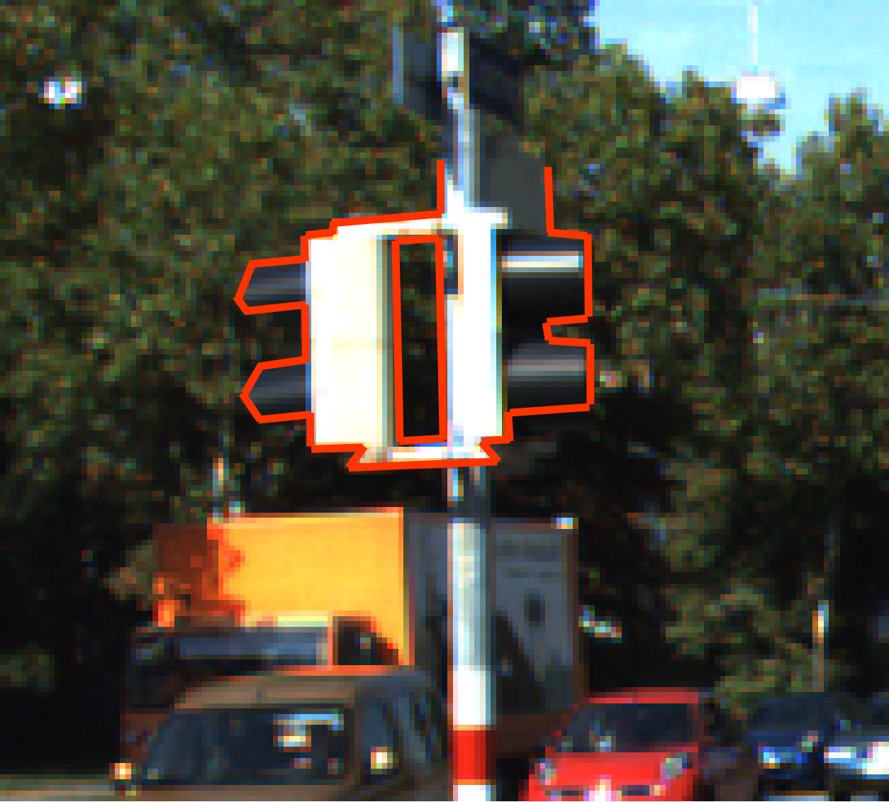
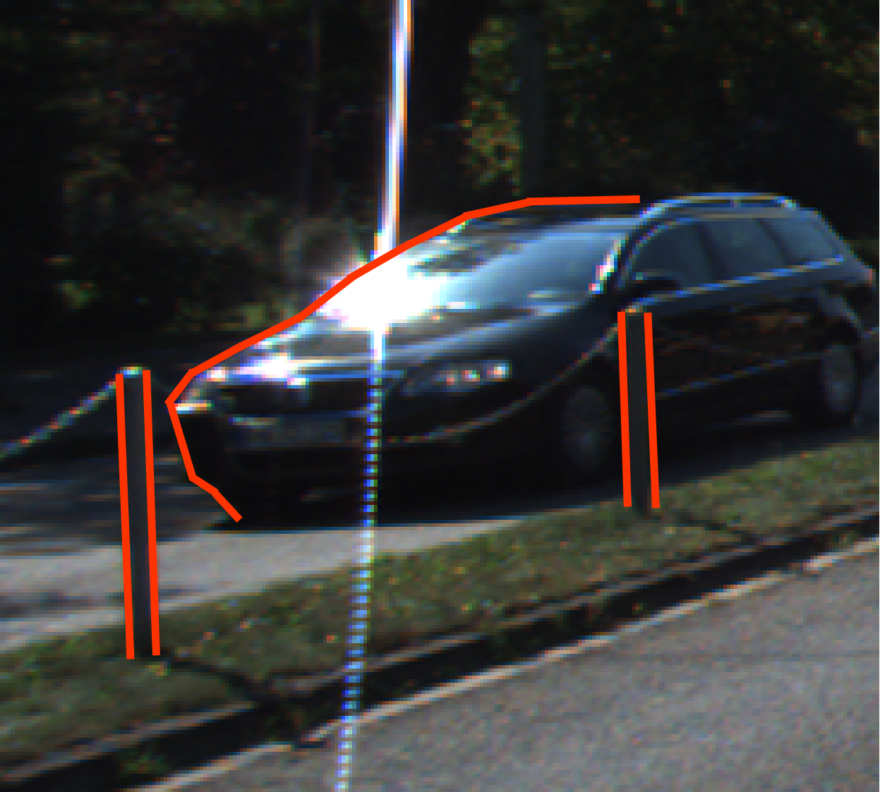
Color Image

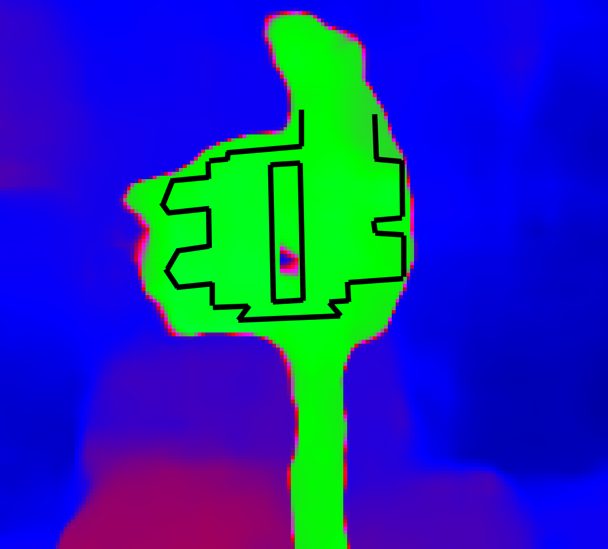
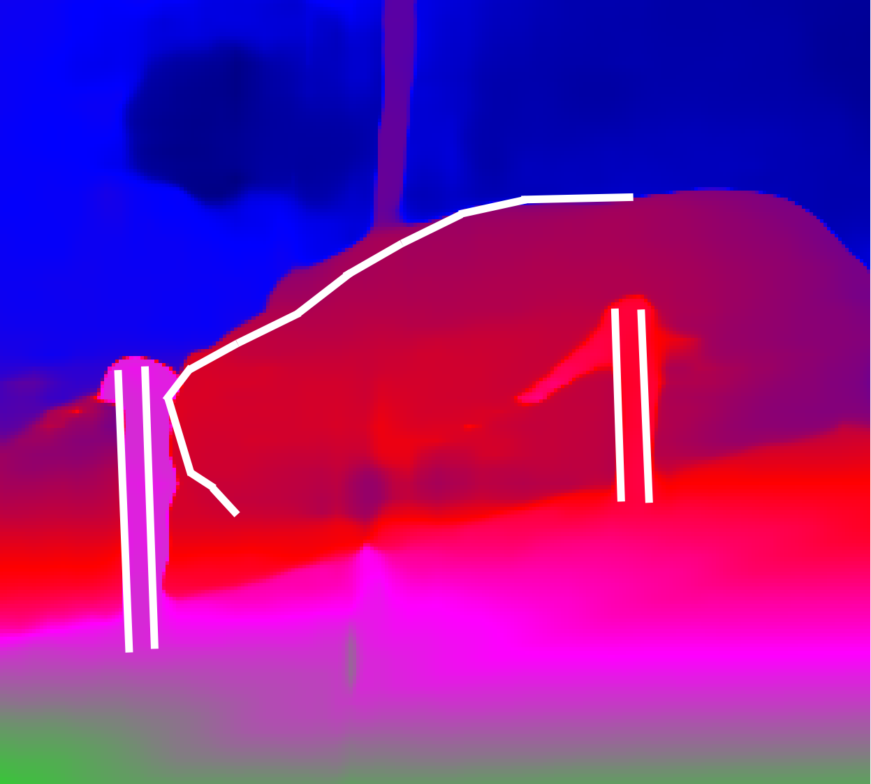
PSMNet

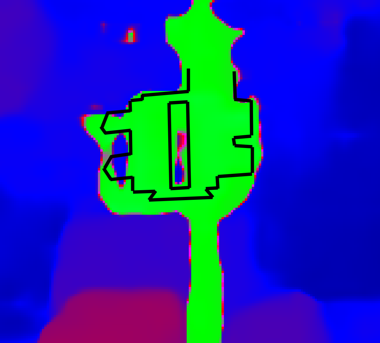
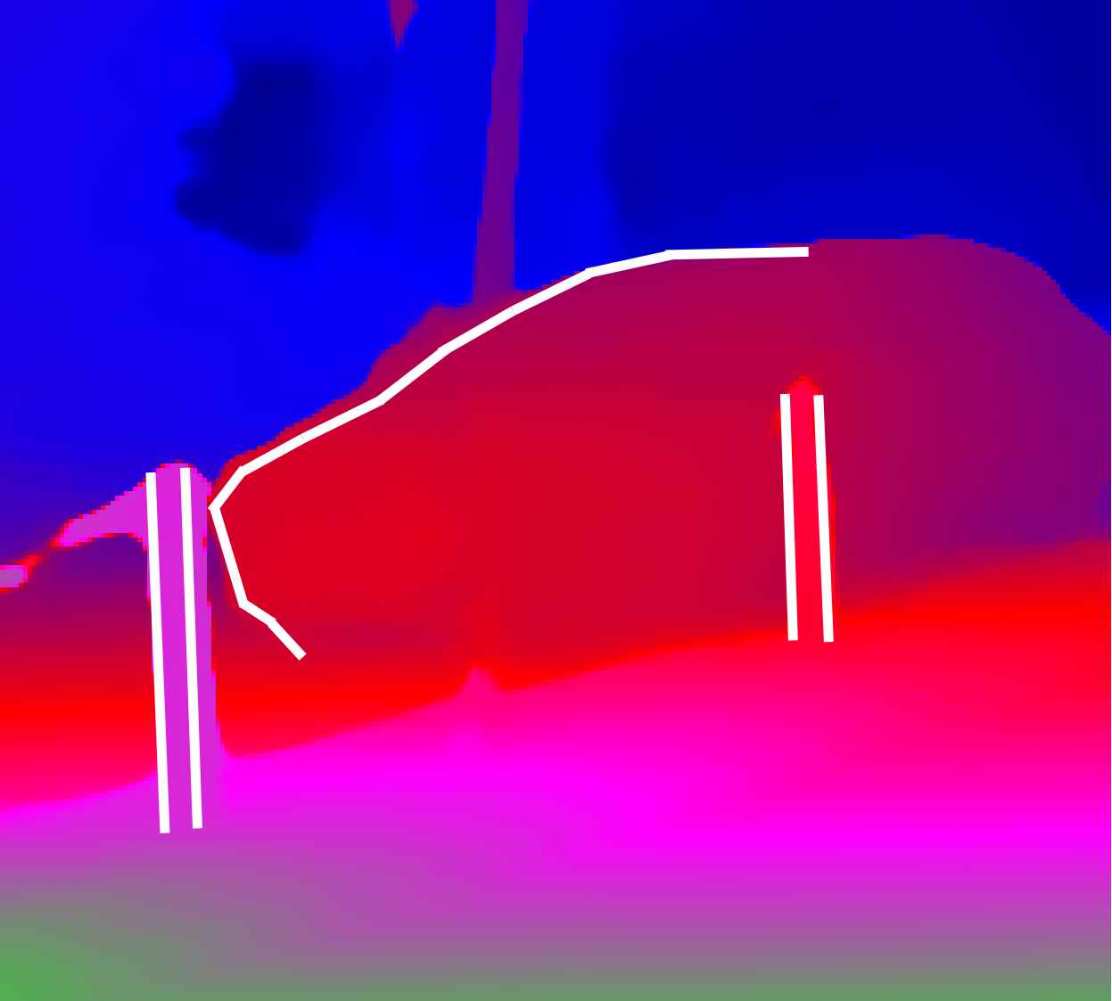
SG-PSMNet

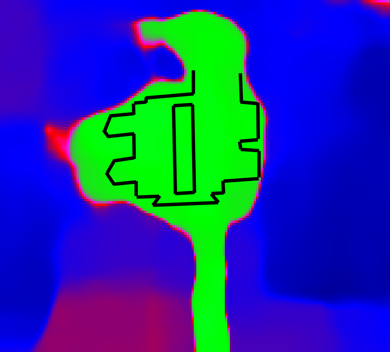
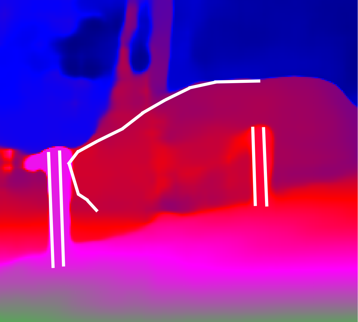
MSN2D

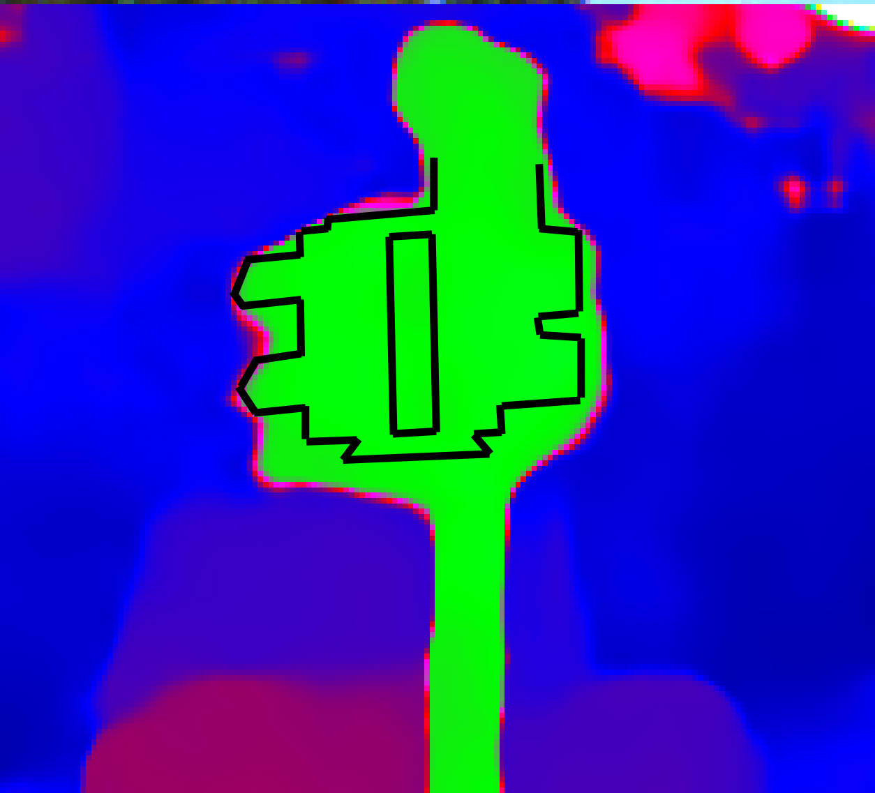
SG-MSN2D

Figure 8: Qualitative comparisons on Kitti2015. We manually marked the outline of the objects for better illustration.

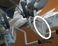
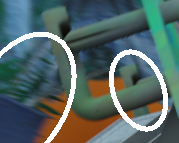
Color Image

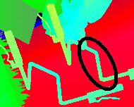
Ground truth

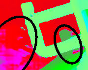
PSMNet

SG-PSMNet

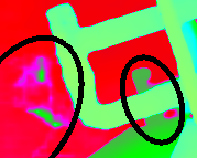
MSN2D

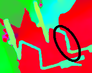
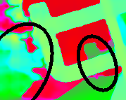
SG-MSN2D

Figure 9: Qualitative comparisons on Sceneflow.

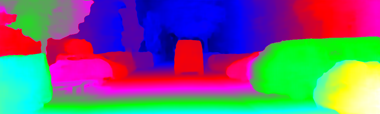
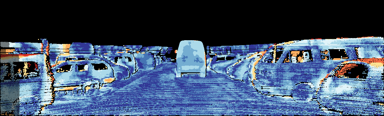
PSMNet

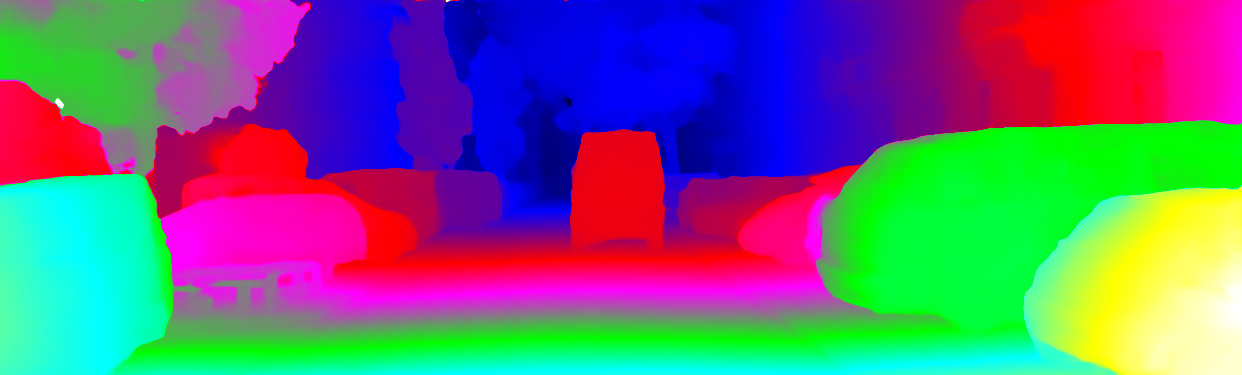
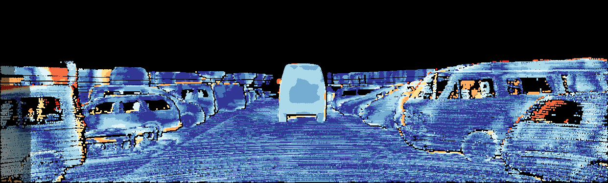
SG-PSMNet

Figure 10: ALL-D1_bg, ALL-D1_fg, ALL-D1_all are PSMNet: ($3.67,1.16,3.45$), SG-PSMNet: ($3.24,1.49,3.08$)

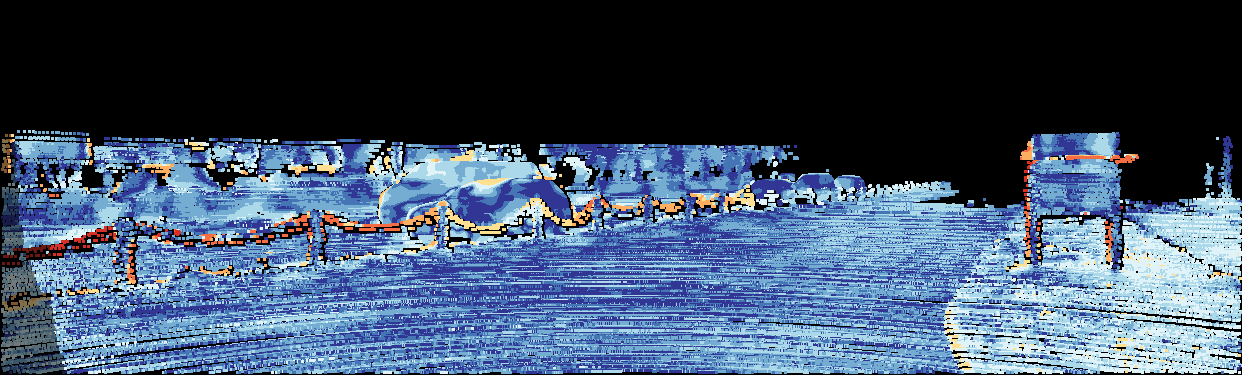
PSMNet

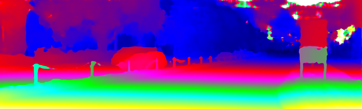
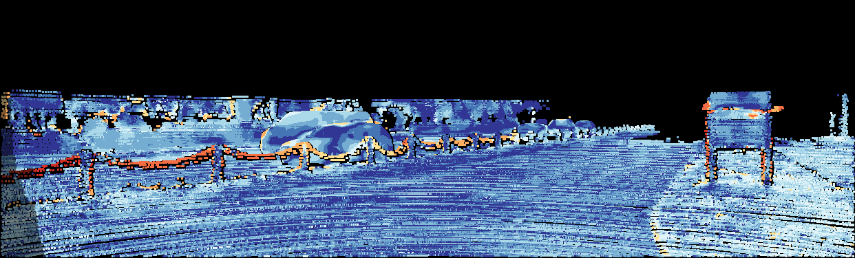
SG-PSMNet

Figure 11: ALL-D1_bg, ALL-D1_fg, ALL-D1_all are PSMNet: ($1.96,2.22,1.99$), SG-PSMNet: ($1.66,0.93,1.58$)

A.7 The results on Kitti2012 and Kitti2015

At last, we provide the URL of our submitted results on Kitti leaderboard. SG-PSMNet on Kitti2015, SG-MSN2D on Kitti2015, SG-MSN3D on Kitti2015, SG-GwcNet-g on Kitti2015, SG-IGEV on Kitti2015. SG-PSMNet on Kitti2012, SG-MSN2D on Kitti2012, SG-MSN3D on Kitti2012, SG-IGEV on Kitti2012.

References

- Bangunharcana et al. (2021) Antyanta Bangunharcana, Jae Won Cho, Seokju Lee, In So Kweon, Kyung-Soo Kim, and Soohyun Kim. Correlate-and-excite: Real-time stereo matching via guided cost volume excitation. In Iros, pp. 3542–3548. IEEE, arXiv, August 2021. arXiv:2108.05773 [cs].
- Chang & Chen (2018) Jia-Ren Chang and Yong-Sheng Chen. Pyramid stereo matching network. arXiv:1803.08669 [cs], pp. 5410–5418, March 2018. arXiv: 1803.08669.
- Chen et al. (2019) Chuangrong Chen, Xiaozhi Chen, and Hui Cheng. On the over-smoothing problem of cnn based disparity estimation. In 2019 IEEE/CVF International Conference on Computer Vision (ICCV), pp. 8996–9004, 2019. doi: 10.1109/ICCV.2019.00909.
- Cheng et al. (2020) Xuelian Cheng, Yiran Zhong, Mehrtash Harandi, Yuchao Dai, Xiaojun Chang, Tom Drummond, Hongdong Li, and Zongyuan Ge. Hierarchical neural architecture search for deep stereo matching. arXiv:2010.13501 [cs], October 2020. arXiv: 2010.13501.
- Geiger et al. (2012) Andreas Geiger, Philip Lenz, and Raquel Urtasun. Are we ready for autonomous driving? the kitti vision benchmark suite. In Conference on Computer Vision and Pattern Recognition (CVPR), 2012.
- Guo et al. (2019) Xiaoyang Guo, Kai Yang, Wukui Yang, Xiaogang Wang, and Hongsheng Li. Group-wise correlation stereo network. arXiv:1903.04025 [cs], March 2019. arXiv: 1903.04025.
- He et al. (2014) Kaiming He, Xiangyu Zhang, Shaoqing Ren, and Jian Sun. Spatial pyramid pooling in deep convolutional networks for visual recognition. In David Fleet, Tomas Pajdla, Bernt Schiele, and Tinne Tuytelaars (eds.), Computer Vision – ECCV 2014, pp. 346–361, Cham, 2014. Springer International Publishing. ISBN 978-3-319-10578-9.
- He et al. (2015) Kaiming He, Xiangyu Zhang, Shaoqing Ren, and Jian Sun. Deep residual learning for image recognition. CoRR, abs/1512.03385, 2015.
- Häger et al. (2021) Gustav Häger, Mikael Persson, and Michael Felsberg. Predicting disparity distributions. In 2021 IEEE International Conference on Robotics and Automation (ICRA), pp. 4363–4369, 2021. doi: 10.1109/ICRA48506.2021.9561617.
- Kendall et al. (2017) Alex Kendall, Hayk Martirosyan, Saumitro Dasgupta, Peter Henry, Ryan Kennedy, Abraham Bachrach, and Adam Bry. End-to-end learning of geometry and context for deep stereo regression. In The IEEE Conference on Computer Vision and Pattern Recognition (CVPR), 2017.
- Li et al. (2021) Jiefeng Li, Tong Chen, Ruiqi Shi, Yujing Lou, Yong-Lu Li, and Cewu Lu. Localization with sampling-argmax. Advances in Neural Information Processing Systems, 34:27236–27248, 2021.
- Liu et al. (2021) Biyang Liu, Huimin Yu, and Yangqi Long. Local similarity pattern and cost self-reassembling for deep stereo matching networks. CoRR, abs/2112.01011, 2021. URL https://arxiv.org/abs/2112.01011.
- Liu & Liu (2022) Jiazhi Liu and Feng Liu. Robust stereo matching with an unfixed and adaptive disparity search range. In 2022 26th International Conference on Pattern Recognition (ICPR), pp. 4016–4022, 2022. doi: 10.1109/ICPR56361.2022.9956286.
- Loshchilov & Hutter (2017) Ilya Loshchilov and Frank Hutter. Fixing weight decay regularization in adam. CoRR, abs/1711.05101, 2017.
- Mayer et al. (2016a) N. Mayer, E. Ilg, P. Häusser, P. Fischer, D. Cremers, A. Dosovitskiy, and T. Brox. A large dataset to train convolutional networks for disparity, optical flow, and scene flow estimation. In The IEEE Conference on Computer Vision and Pattern Recognition (CVPR), June 2016a. arXiv:1512.02134.
- Mayer et al. (2016b) Nikolaus Mayer, Eddy Ilg, Philip Häusser, Philipp Fischer, Daniel Cremers, Alexey Dosovitskiy, and Thomas Brox. A large dataset to train convolutional networks for disparity, optical flow, and scene flow estimation. 2016 IEEE Conference on Computer Vision and Pattern Recognition (CVPR), pp. 4040–4048, 2016b. doi: 10.1109/cvpr.2016.438. arXiv: 1512.02134.
- Menze & Geiger (2015) Moritz Menze and Andreas Geiger. Object scene flow for autonomous vehicles. In The Conference on Computer Vision and Pattern Recognition (CVPR), 2015.
- Nibali et al. (2018) Aiden Nibali, Zhen He, Stuart Morgan, and Luke A. Prendergast. Numerical coordinate regression with convolutional neural networks. CoRR, abs/1801.07372, 2018. URL http://arxiv.org/abs/1801.07372.
- Pan et al. (2020) Baiyu Pan, Liming Zhang, and Hanzi Wang. Multi-stage feature pyramid stereo network based disparity estimation approach for two to three-dimensional video conversion. IEEE Transactions on Circuits and Systems for Video Technology, pp. 1–1, 2020. ISSN 1051-8215, 1558-2205. doi: 10.1109/tcsvt.2020.3014053.
- Pan et al. (2024) Baiyu Pan, Jichao Jiao, Jianxing Pang, and Jun Cheng. Distill-then-prune: An efficient compression framework for real-time stereo matching network on edge devices. In 2024 IEEE International Conference on Robotics and Automation (ICRA), pp. 15113–15120, 2024. doi: 10.1109/ICRA57147.2024.10611085.
- Shamsafar et al. (2021) Faranak Shamsafar, Samuel Woerz, Rafia Rahim, and Andreas Zell. Mobilestereonet: Towards lightweight deep networks for stereo matching. arXiv:2108.09770 [cs], August 2021. arXiv: 2108.09770.
- Shen et al. (2023) Zhelun Shen, Xibin Song, Yuchao Dai, Dingfu Zhou, Zhibo Rao, and Liangjun Zhang. Digging into uncertainty-based pseudo-label for robust stereo matching. IEEE Transactions on Pattern Analysis and Machine Intelligence, 2023.
- Teed & Deng (2021) Zachary Teed and Jia Deng. Raft-3d: Scene flow using rigid-motion embeddings. In Proceedings of the IEEE/CVF conference on computer vision and pattern recognition, pp. 8375–8384, 2021.
- Tulyakov et al. (2018) Stepan Tulyakov, Anton Ivanov, and François Fleuret. Practical deep stereo (PDS): toward applications-friendly deep stereo matching. CoRR, abs/1806.01677, 2018. URL http://arxiv.org/abs/1806.01677.
- Wang et al. (2021) Hengli Wang, Rui Fan, Peide Cai, and Ming Liu. Pvstereo: Pyramid voting module for end-to-end self-supervised stereo matching. IEEE Robotics and Automation Letters, 6(3):4353–4360, 2021.
- Xu et al. (2022) Gangwei Xu, Junda Cheng, Peng Guo, and Xin Yang. Attention concatenation volume for accurate and efficient stereo matching. In Proceedings of the IEEE/CVF Conference on Computer Vision and Pattern Recognition, pp. 12981–12990. arXiv, June 2022. doi: 10.48550/arXiv.2203.02146. arXiv:2203.02146 [cs].
- Xu et al. (2023) Gangwei Xu, Xianqi Wang, Xiaohuan Ding, and Xin Yang. Iterative geometry encoding volume for stereo matching. In Proceedings of the IEEE/CVF Conference on Computer Vision and Pattern Recognition, June 2023.
- Xu et al. (2024a) Gangwei Xu, Xianqi Wang, Zhaoxing Zhang, Junda Cheng, Chunyuan Liao, and Xin Yang. Igev++: Iterative multi-range geometry encoding volumes for stereo matching. arXiv preprint arXiv:2409.00638, 2024a.
- Xu & Zhang (2020) Haofei Xu and Juyong Zhang. Aanet: Adaptive aggregation network for efficient stereo matching. In 2020 IEEE/CVF Conference on Computer Vision and Pattern Recognition (CVPR), pp. 1956–1965, Seattle, WA, USA, June 2020. Ieee. ISBN 978-1-72817-168-5. doi: 10.1109/cvpr42600.2020.00203.
- Xu et al. (2024b) Peng Xu, Zhiyu Xiang, Chengyu Qiao, Jingyun Fu, and Tianyu Pu. Adaptive multi-modal cross-entropy loss for stereo matching. In Proceedings of the IEEE/CVF Conference on Computer Vision and Pattern Recognition (CVPR), pp. 5135–5144, June 2024b.
- Zhang et al. (2019a) Feihu Zhang, Victor Adrian Prisacariu, Ruigang Yang, and Philip H. S. Torr. Ga-net: Guided aggregation net for end-to-end stereo matching. CoRR, abs/1904.06587, 2019a.
- Zhang et al. (2019b) Youmin Zhang, Yimin Chen, Xiao Bai, Jun Zhou, Kun Yu, Zhiwei Li, and Kuiyuan Yang. Adaptive unimodal cost volume filtering for deep stereo matching. CoRR, abs/1909.03751, 2019b. URL http://arxiv.org/abs/1909.03751.