An X-ray Shell Reveals the Supernova Explosion for Galactic Microquasar SS 433

Abstract

How black holes are formed remains an open and fundamental question in Astrophysics. Despite theoretical predictions, it lacks observations to understand whether the black hole formation experiences a supernova explosion. Here we report the discovery of an X-ray shell north of the Galactic micro-quasar SS 433 harboring a stellar-mass black hole spatially associated with radio continuum and polarization emissions, and an HI cloud. Its spectrum can be reproduced by a 1-keV under-ionized plasma, from which the shell is inferred to have been created by a supernova explosion 20–30 kyr ago and its properties constitute evidence for canonical SN explosions to create some black holes. Our analysis precludes other possible origins including heated by jets or blown by disk winds. According to the lower mass limit of the compact object in SS 433, we roughly deduced that the progenitor should be more massive than 25 M_⊙. The existence of such a young remnant in SS 433 can also lead to new insights into the supercritical accretion in young microquasars and the $\gamma$-ray emission of this system. The fallback ejecta may provide accretion materials within tens of thousands of years while the shock of the supernova remnant may play a crucial role in the cosmic ray (re)acceleration.

1 Introduction

The young ($10^{4}-10^{5}$ yr, Zealey et al., 1980; Shkovskii, 1981; van den Heuvel, 1981; Lockman et al., 2007; Goodall et al., 2011; Panferov, 2017) high-mass X-ray binary SS 433 is a famous system with relativistic jets and may be the only Galactic prototype of an ultra-luminous X-ray source (Brinkmann et al., 2007; Safi-Harb et al., 2022). SS 433 stands out from many other X-ray binaries due to its supercritical gas accretion onto a compact object, where the mass-accretion rate greatly exceeds the Eddington rate, defined by balancing the radiation pressure with gravity. The mass of the compact object remains uncertain despite decades of study, but the latest results suggest a high mass ratio of the compact object to the donor star of $q\gtrsim 0.6$ and a compact object mass of 5–15 M_⊙, favoring a stellar black hole over a neutron star (Gies et al., 2002; Bowler, 2018; Cherepashchuk et al., 2019). This energetic system is known to strongly modify its surroundings. SS 433 is harbored within a giant radio nebula, W50 referred to as the Manatee nebula, with an angular size 2°$\times$1° (174 pc$\times$87 pc at a distance of 5 kpc, Su et al., 2018) (Dubner et al., 1998), whose major axis from west to east aligns to the X-ray lobes shaped by the relativistic jets (Figure 1). Perpendicular to the collimated jets, W50 still has a remarkable extension of 1°, requiring other mechanisms to drive the bubble, such as an SNR, equatorial disk winds, or different jet episodes in the past (Fabrika, 2004; Goodall et al., 2011; Farnes et al., 2017). The physical nature of W50 thus links some crucial questions on stellar-mass black holes, the most extreme stellar objects in our Universe: Was the black hole created with an SN explosion? What is the feedback and evolution of a microquasar? Past observations focused primarily on the bright non-thermal X-ray lobes which probe the impact of the jets with the W50 nebula in the east-west direction (Brinkmann et al., 2007; Safi-Harb et al., 2022). With the new XMM-Newton observations, we target the perpendicular direction where other mechanisms may stand out free from contamination by the luminous jets. As such, we conduct the first search and study of the X-ray emission in the northern region of W50 and outside the precession cone of SS 433.

This letter is organized as follows: we present our analysis based on XMM-Newton observations and the newly discovered X-ray shell in §2 and §3, respectively. Then we discuss its origin as an SNR (§4.1), the mass of the supernova progenitor (§4.2), and the new insights the SNR brings us on the supercritical accretion (§4.3) and $\gamma$-ray emission of SS 433/W50 system (§4.4).

2 XMM-Newton observations and data reduction

The North of W50 was observed by XMM-Newton (Jansen et al., 2001) in Oct. 2021 and Apr. 2022 (ObsID: 0882560201 and 0882560101, PI: P. Zhou). Observation 0882560201 was heavily contaminated by soft proton flares, leading to a reduced flare-free exposure time of 19.6, 23.5, and 9.6 ks for MOS1 (Turner et al., 2001), MOS2, and pn camera (Strüder et al., 2001), respectively. We mainly used observation 0882560101 pointing to W50 Northeast, whose flare-filtered exposure is 40.9, 40.4, and 33.2 ks for three instruments. We retrieved archival XMM-Newton data of SS 433 (0694870201, PI: A. Medvedev) and the luminous jet lobes (0840490101, PI: S. Safi-Harb; 0075140401 and 0075140501, PI: W. Brinkmann) for a large-scale X-ray image of W50. We reproduced and analyzed XMM-Newton observations with the XMM-Newton Science Analysis System (SAS, version 20.0, Gabriel et al., 2004) and the XMM-Newton Extended Source Analysis Software (XMM-ESAS, version 0.11.2) for the background modeling (Snowden et al., 2004). All the raw data are reprocessed by emchain and epchain, and then the contamination of flares is filtered using mos-filter and pn-filter.

3 Results

3.1 Morphology

We selected the 0.4–1.2 keV and 2.0–5.0 keV bands for imaging analysis, where the softer band traces thermal emission from hot plasma and where the non-thermal synchrotron emission dominates the harder X-ray band. The intermediate energy band was excluded to avoid the strong instrumental Al K (1.49 keV, for MOS and pn) and Si K (1.75 keV, for MOS) lines. For each observation, mos-spectra and pn-spectra produce images and exposure maps in the two selected bands for each camera. The instrumental background of each image, or rather, quiescent particle background (QPB), is modeled through mos_back or pn_back and projected to the sky by rot-im-det-sky. All the images, exposure maps, and QPB backgrounds were mosaicked using merge_comp_xmm. To underline the faint structure of the diffuse emission, we applied the task cheese to detect and mask point-like sources in each band and subsequently adaptively binned the image based on Weighted Voronoi Tessellation algorithm (Cappellari & Copin, 2003; Diehl & Statler, 2006) to ensure an average signal-to-noise ratio of 10 per bin. The dual-band false-color image (Figure 1) shows the heated gas (red) and synchrotron emission of the jet (cyan).

A shell-like structure appears northeast of SS 433 in the 0.4–1.2 keV band (Figure 1 & 2(a)). Although fainter than in the jet-impact areas in the east and west, the X-ray structure is clearly detected and spatially correlated with the radio shell in the north. The emission of this structure above 2 keV is too weak to be detected in that band, indicative of a soft X-ray spectrum. Figure 2 provides a close-up image of the northern X-ray shell (a), in comparison with the radio emission (b), polarized radio signal (c), and the HI gas (d). The shell has a curvature radius of $\sim 20^{\prime}$ and is roughly centered at the position of SS 433. An X-ray-enhanced clump appears in the north, where the radio emission is locally enhanced (Dubner et al., 1998) and highly polarized (Gao et al., 2011; Farnes et al., 2017). Meanwhile, the X-ray clump is spatially associated with an HI cloud at a distance of $\sim 5$ kpc (Su et al., 2018), probably indicative of a density enhancement due to an interaction with the HI cloud.

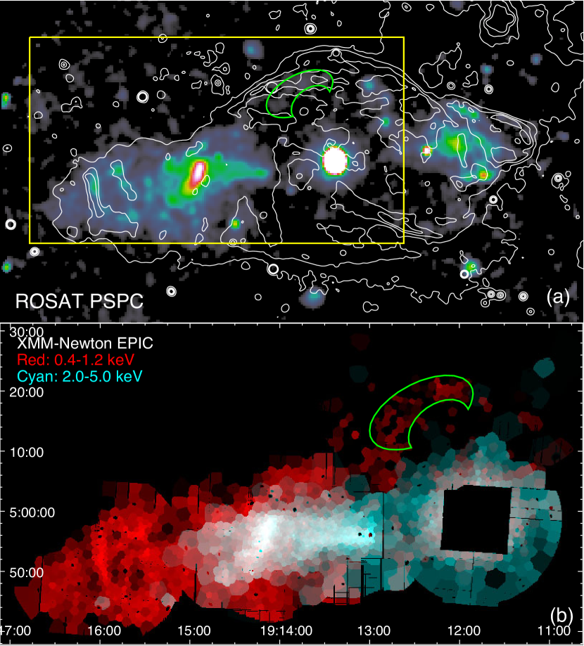
Figure 1: Location of the X-ray shell. (a): ROSAT PSPC X-ray image (see Appendix A) of the nebula W50 overlapped by the intensity contour of the 1.4 GHz VLA observation (Dubner et al., 1998). (b): Zoom-in dual-band XMM-Newton image in the region marked in yellow in 0.4–1.2 keV (red) and 2.0–5.0 keV (cyan) with point-like sources subtracted. Each bin shares an average signal-to-noise ratio of 10. The softer and harder energy bands highlight the thermal and non-thermal emission of the nebula, respectively. The green region labels the shell-like structure.

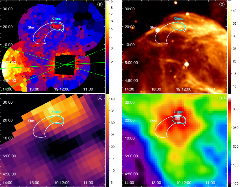
Figure 2: Zoom-in multi-band images of our region of interest. (a): XMM-Newton EPIC 0.4–1.2 keV mosaic in units of counts deg^-2 s^-1. Each bin has a signal-to-noise ratio of $\sim 10$. The X-ray shell and clump are labeled in white and cyan, respectively. The green solid and dashed lines mark the jet axis and cone of the jet precession and nod, respectively (Fabrika, 2004). (b): VLA 1.4 GHz intensity map in units of mJy/beam (Dubner et al., 1998). (c): Sino-German 6 cm polarized fraction map in units of percentage. (Gao et al., 2011) (d): Acrecibo HI intensity in 68–75 km s^-1 in units of K (Peek et al., 2018; Su et al., 2018).

3.2 Spectral Analysis

We analyze the spectra of the whole northern X-ray shell ($\sim 9.4^{\prime}\times 4.9^{\prime}$, defined as “Shell”) and the sub-structure clump ($\sim 3.9^{\prime}\times 2.0^{\prime}$, defined as “Clump”). The source regions are shown in Figure 2 and the sky background is selected outside the radio boundary of W50. The instrumental background matters, especially when analyzing weak diffuse emission and when the instrumental background is non-uniform across the field of view. Therefore, instead of directly subtracting the sky background, we obtained the sky background model by fitting the QPB-subtracted background spectra and applied the model to the source spectra by multiplying an area ratio between the source and background regions. The task mos-spectra and pn-spectra extracted spectra and generated response files, while the QPB spectra of each region are modeled by mos_back and pn_back. The spectra were grouped with ftgrouppha to guarantee at least 50 counts per bin in favor of chi-square statistics. XSPEC (version 12.13.0c, Arnaud, 1996) with AtomDB (version 3.0.9) was used for spectral analysis. The fitting parameters are listed in Table 1 and spectra with folded models are shown in Appendix B.

Table 1: XMM-Newton X-ray spectral fitting results. The errors correspond to 1$\sigma$ uncertainties.

Region	Absorption	plasma								$\chi^{2}$/d.o.f.
	$N_{\rm H}$	model	kT	$\tau$	norm	O	Ne	Mg	Si
	$10^{21}\rm\,cm^{-2}$		keV	$10^{10}$ s cm-3	$10^{-4}\rm\,cm^{-5}$	Z/Z⊙	Z/Z⊙	Z/Z⊙	Z/Z⊙
Shell	$6.61_{-0.81}^{+0.90}$	vnei	$1.23_{-0.33}^{+0.58}$	$2.6_{-0.9}^{+1.9}$	$1.27_{-0.31}^{+0.51}$	$\cdots$	$\cdots$	$1.22_{-0.28}^{+0.33}$	$2.64_{-0.60}^{+0.77}$	546.8/467
	$6.9_{-2.7}^{+1.9}$	vpshock	$1.1_{-0.3}^{+1.0}$	$5.2_{-3.2}^{+10.0}$	$1.63_{-0.81}^{+0.98}$	$0.84_{-0.58}^{+1.02}$	$\cdots$	$1.21_{-0.34}^{+0.49}$	$3.03_{-0.84}^{+0.65}$	547.7/466
	$4.87_{-0.89}^{+0.74}$	vapec	$0.77_{-0.03}^{+0.04}$	$\cdots$	$1.62_{-0.28}^{+0.31}$	$9.4_{-2.7}^{+3.1}$	$\cdots$	$3.3_{-1.1}^{+1.4}$	$3.5_{-1.0}^{+1.1}$	547.4/467
	$5.1_{-1.9}^{+1.2}$	vapec*	$0.74_{-0.04}^{+0.05}$	$\cdots$	$2.07_{-0.74}^{+0.70}$	$\cdots$	$\cdots$	$3.4_{-1.1}^{+2.1}$	$3.5_{-1.0}^{+1.8}$	561.7/468
	$\cdots$	Null	$\cdots$	$\cdots$	$\cdots$	$\cdots$	$\cdots$	$\cdots$	$\cdots$	763.9/472
Clump	$10.3_{-1.6}^{+1.9}$	vnei	$0.8_{-0.3}^{+1.1}$	$1.0_{-0.3}^{+4.8}$	$1.4_{-1.1}^{+2.9}$	$\cdots$	$\cdots$	$1.07_{-0.33}^{+0.39}$	$2.2_{-1.3}^{+2.4}$	195.5/162
	$8.3_{-2.8}^{+8.1}$	vpshock	$0.92_{-0.70}^{+0.78}$	$3.1_{-1.7}^{+9.7}$	$0.8_{-0.5}^{+2.5}$	$0.6_{-0.4}^{+1.0}$	$\cdots$	$1.25_{-0.67}^{+0.64}$	$1.8_{-1.0}^{+2.7}$	194.9/161
	$4.9_{-1.7}^{+1.6}$	vapec	$0.74_{-0.07}^{+0.07}$	$\cdots$	$0.55_{-0.19}^{+0.30}$	$5.9_{-3.6}^{+4.6}$	$<4.5$	$3.8_{-1.7}^{+2.8}$	$1.8_{-1.4}^{+2.0}$	200.4/161
	$6.3_{-2.1}^{+1.6}$	vapec*	$0.71_{-0.06}^{+0.07}$	$\cdots$	$0.86_{-0.33}^{+0.41}$	$\cdots$	$\cdots$	$2.9_{-1.2}^{+2.2}$	$1.5_{-0.9}^{+1.3}$	202.5/163
	$\cdots$	Null	$\cdots$	$\cdots$	$\cdots$	$\cdots$	$\cdots$	$\cdots$	$\cdots$	294.9/167

When fitting the sky background, we considered the X-ray emission from the local hot bubble (apec), Galactic ISM (vapec), and background AGN (powerlaw with a photon index of 1.4, Chen et al., 1997) (Snowden et al., 2004; Kuntz & Snowden, 2008). To further mimic the spectra, we let the abundances of vapec vary and got a reduced chi-square ($\chi^{2}_{r}$) of 0.98 with 191 degrees of freedom. For source spectra, apart from the sky background, we tested four different models, including powerlaw (for non-thermal emission), vapec (plasma in collision-ionization-equilibrium, CIE, Smith et al., 2001), vnei (non-equilibrium ionization, NEI, plasma), and vpshock (plane-parallel shocked non-equilibrium plasma, Borkowski et al., 2001). The absorption component of all these models is TBabs (Wilms et al., 2000).

The non-thermal model gives a high or steep photon index $\Gamma$ of $5.71_{-0.55}^{+0.66}$ for the Shell at a confidence level of 1$\sigma$, much higher than the synchrotron emission detected in the lobes ($\Gamma\approx 1.6$, Safi-Harb et al., 2022; Brinkmann et al., 2007) and a typical value of $<3$ for non-thermal objects. In contrast, such a photon index suggests a soft spectrum probably dominated by thermal X-ray emission. Meanwhile, the reduced chi-square is 1.31 with 470 degrees of freedom, significantly poorer than any other model. The NEI models, vnei and vpshock, are widely used to describe X-ray plasmas in SNRs (Borkowski et al., 2001). Limited by the count rate, we are unable to distinguish between these two NEI models statistically with current data. The fitting result generally supports a hot plasma with a temperature $kT\sim 1$ keV and an ionization timescale $n_{e}t\sim 10^{10}$ s cm^-3 for both two regions. The abundance of Si is over twice the solar abundance (Wilms et al., 2000) for the best-fit model of the Shell, while that of O and Mg are near solar. For the Clump, the abundance seems to be similar but cannot be well constrained. A model describing plasma in CIE is also tested for these two regions. The best-fit CIE model gives similar fitting statistics to the NEI models but needs a very high metal abundance, especially for O and Mg, which often appears in the metal-rich ejecta of young or middle-aged SNRs (see Vink, 2020, and references therein). As O lines (0.5–0.7 keV) are dominated by astrophysical background compared to Mg ($\sim 1.3$ keV) and Si ($\sim 1.8$ keV) lines (see spectra in Appendix B), we also fix O to solar abundance in CIE, named vapec* in Table 1, and use F-test to test the significance of the under-ionization state (i.e. vnei versus vapec). We noticed that a deviation from CIE is significant for the Shell with a null hypothesis probability of $4\times 10^{-4}$, while for the Clump this improvement is less evident (probability $\sim 0.017$). Therefore, we are in favor of the NEI model here but the CIE model cannot be completely excluded from fitting statistics as the ionization timescale and metal abundances need further constraints in the future study. Meanwhile, as the diffuse emission has a low surface brightness, we also consider the “null hypothesis” where the emission is dominated by background fluctuation (i.e. fix the sky background and free its normalization instead of weighting by the sky area) as listed in Table 1. This along with further analysis on the lower limit of the norm parameter indicates a robust detection of the diffuse emission (see Appendix C for details).

4 Discussion

4.1 Origin of the X-ray shell

The newly discovered X-ray shell north of SS 433 is not only much dimmer than the X-ray lobes but also composed of hot and under-ionized plasma, while the thermal emission of the lobe is much cooler ($<0.3$ keV) and close to CIE (Safi-Harb et al., 2022). Thus, we tend to exclude the possibility that the X-ray shell was heated by the past relativistic jet with an extreme precession angle up to $\sim 90^{\circ}$, as we would expect a cooler and CIE plasma as found in bipolar X-ray lobes (Safi-Harb et al., 2022). Moreover, the radio polarization measurement of this region reveals tangential magnetic fields in the northern shell and a high polarization degree up to $\sim 50\%$ (Gao et al., 2011; Farnes et al., 2017), while magnetic fields in the jet region are found to align parallel to the jet direction (Kaaret et al., 2023). As observed in several old SNRs, highly ordered magnetic fields along the shell can be produced by a compression of the ambient gas by shocks (Gao et al., 2011; Dubner & Giacani, 2015). Considering the spectroscopy and polarization properties, we suggest that the X-ray shell has a different physical origin from the elongated jet-blown lobes, but shows properties consistent with an SNR.

Based on the spectral fittings of the X-ray shell with an NEI model, we estimate its average density to be $\sim 0.03$ cm^-3. This is lower than that of the terminal shock of the eastern lobe ($\sim 1$ cm^-3, Safi-Harb et al., 2022), showing that the gas density in the direction along and perpendicular to the jets is different. The high temperature, low density, and faint optical emission (Boumis et al., 2007; Farnes et al., 2017) here suggest that the remnant is still in a Sedov-Taylor phase (Taylor, 1950; Sedov, 1959). Under this assumption, we deduce that its age is $\sim 17$–29 kyr and the explosion energy is $\sim 0.4$–$1.4\times 10^{51}$ erg (see details in Appendix D), a typical value for a core-collapse SN. The super-solar abundance of Si has previously been found in the outflowing matter of SS 433 (Brinkmann et al., 2005), further supporting the existence of chemical enrichment near SS 433 by an SNR.

Another potential physical origin of the X-ray shell could be the equatorial wind from the supercritical accretion disk (Shakura & Sunyaev, 1973; Churazov et al., 2024), where fast winds have been observed with optical or radio observations (Waisberg et al., 2019; Paragi et al., 1999). We estimate the power of the equatorial wind as $\sim 3\times 10^{37}$ erg s^-1, based on a mass loss rate of the gas flow of $10^{-4}$ M_⊙ yr^-1 (van den Heuvel, 1981; Shkovskii, 1981; Fuchs et al., 2006) and an average wind terminal velocity of 1000 km s^-1 (Fabrika, 1997). This power is optimistically high since the wind velocity drops dramatically to $\sim 100$ km s^-1 in areas perpendicular to the jet (Fabrika, 2004). Nevertheless, the wind power is much smaller than $\sim 10^{39}$ erg s^-1, the “average power” of a $\sim 20$-kyr SNR. Based on a self-similar solution of wind bubble (Weaver et al., 1977; Mac Low & McCray, 1988), the plasma would be much cooler ($\sim 0.2$ keV) than the fitting result. To further assess this wind scenario, we simulate the evolution of an isotropic wind driven from SS 433 into a uniform diffuse medium with a density of 0.01 cm^-3 and also consider a dense cloud in a distance of 40 pc to mimic the dense-gas conditions near the Clump. The snapshot of the distribution of density, temperature, and estimated surface brightness at the age of 20, 95, and 150 kyr are shown in Figure 3. For the estimation of the power of wind and supernova along with the details of the simulation, see Appendix E.

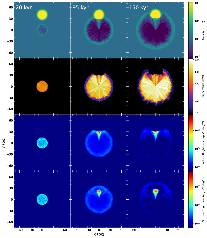
Figure 3: Evolution of a bubble powered by isotropic disk winds with a power of $3\times 10^{37}$ erg s^-1 within a uniform medium and a dense cloud in the north. From top to bottom rows show the evolution of the density, temperature, and the X-ray surface brightness in 0.4–2.5 keV. The bottom panels give the surface brightness evolution for the case where the cloud is rotated 41.4^∘ towards us (so that it is projected 30 pc north of SS 433). From left to right, the age of the wind bubble is 20, 95, and 150 kyr, respectively, corresponding to the age of the SNR, the beginning of the collision with the dense cloud, and the later evolution of the wind bubble.

Our simulation shows that it would take $\sim 95$ kyr for the winds to blow out a cavity with a radius of the minor axis of W50. The challenge is that the wind is not strong enough for the observed X-ray flux and the gas temperature. The brightest emission appears where the winds interact with the cloud, but the surface brightness is still only half of the observed value of the Clump especially when projection effects are taken into consideration (see Appendix E for more details). Without a wind-cloud interaction, other parts of the wind bubble are significantly fainter than the region Shell. Besides, we found that the temperature of the wind bubble is inconsistent with the observation. At around 95 kyr, the bubble shell has a temperature of $\lesssim 0.5$ keV (see Figure 3), significantly cooler than that obtained from the observation. Theoretically, the temperature of the wind shell declines with the age due to the adiabatical cooling (see Equation E4). The shell thus should be hotter at an earlier age, and the simulation gives an effective temperature (emissivity-weighted) of $\sim 0.6$ keV for the shell at 20 kyr. At the wind-cloud interaction region where X-rays are enhanced, the effective temperature is less than 0.6 keV, either in the surface brightness peak ($\sim 90$ kyr) or later evolution (150 kyr as an example). Moreover, a longer evolution timescale of the wind compared to the SNR scenario suggests likely a larger ionization timescale so that the plasma could be in or close to the CIE state. Therefore, we conclude that the equatorial disk wind cannot describe the shell-like X-ray emission north of SS 433.

4.2 Progenitor mass of the compact object in SS 433

As shown above, an SNR provides the best explanation for the newly discovered X-ray structure. Our X-ray study and the previously measured black hole mass of 5–15 M_⊙ in SS 433 (Cherepashchuk et al., 2019; Bowler, 2018; Gies et al., 2002) provide crucial information about the initial stellar mass and the SN properties for creating a black hole. Here we discuss the progenitor mass of the black hole in SS 433 using the pre-SN core mass as predicted by the stellar evolution models (Sukhbold et al., 2016; Woosley & Heger, 2015; Sukhbold & Woosley, 2014; Woosley & Heger, 2007) along with core-collapse SN explosion models (Zhang et al., 2008; Sukhbold et al., 2016; Fryer et al., 2018). Figure 4 shows the pre-SN He core masses and the compact remnant mass as a function of the zero-age main-sequence stellar mass for stars with solar metallicity.

Previous studies suggest that the He core mass sets the upper limit of the compact object mass (Zhang et al., 2008; Sukhbold et al., 2016). For stars with initial mass ranging from 15 to 30 M_⊙, we fitted the data given by Sukhbold et al. (2016) and found that there exists an approximate linear relation between stellar initial mass $M_{\mathrm{ZAMS}}$ and the final mass of He core $M_{\mathrm{He}}$:

$$M_{\mathrm{ZAMS}}\approx 2.44M_{\mathrm{He}}+4.75\,\mathrm{M_{\odot}}.$$ (1)

Above $\sim 40$ M_⊙, the massive star strips most of the envelope mass with strong stellar winds and ends with an intermediate-mass core. To create a 5-M_⊙ compact object needs a progenitor star more massive than $\sim 17$ M_⊙, while a 10-M_⊙ compact object infers the progenitor mass range of $\sim 30-50$ M_⊙. Nevertheless, this estimate can be oversimplified as it does not consider the metal masses taken away by SN ejecta or the explosion parameters that significantly influence the final remnant mass.

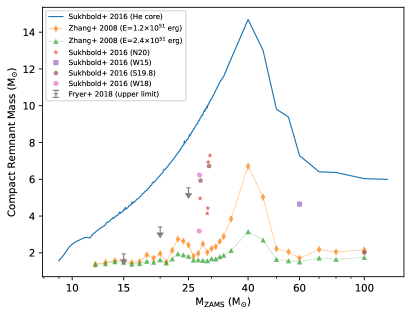
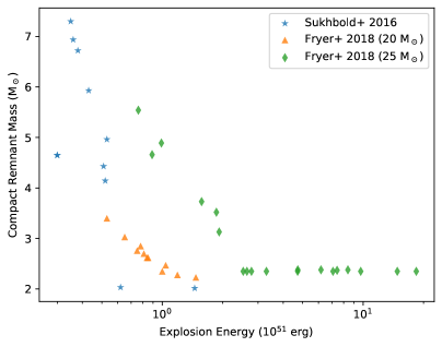
Figure 4: Left panel: mass “budget” of the compact object. The blue solid line represents the mass of He core (Sukhbold et al., 2016). Yellow diamonds and green triangles correspond to models with a given explosion energy (Zhang et al., 2008). Grey scatters label the maximum compact remnant mass among different explosion parameters with a given progenitor mass (Fryer et al., 2018). The others are adopted from 4 different central engines (Sukhbold et al., 2016) and only cases with a compact object mass over 2 M_⊙ are shown here. Right panel: mass of black holes with successful supernova explosion as a function of the explosion energy. Blue stars are given by Sukhbold et al. (2016), while orange triangles (20 M_⊙) and green diamonds (25 M_⊙) are from Fryer et al. (2018). Only cases where the black hole mass exceeds 2  M_⊙ are reserved.

Theoretical studies predict a wide diversity of SNe from these very massive stars, from failed SNe (stars quietly collapse to black holes, Kochanek, 2014) to “hypernovae” with $E_{\rm SN}\gtrsim 10^{52}$ erg (Nomoto et al., 2013). To explore the dependence of the compact remnant mass on the explosion energy, we adopt the predicted results from three SN explosion models for stars with solar metallicities (Zhang et al., 2008; Sukhbold et al., 2016; Fryer et al., 2018). Two of these models are taken from Zhang et al. (2008) for explosion energies of $\sim 1.2\times 10^{51}$ erg and $\sim 2.4\times 10^{51}$ erg. Four models from Sukhbold et al. (2016) applied different central engines (N20 (Nomoto & Hashimoto, 1988), W15 (Woosley et al., 2002), S19.8 (Woosley et al., 2002), and W18 (Sukhbold et al., 2016)) and provide a range of explosion energies (we only take those producing a remnant mass over 2.5 M_⊙ and with SN explosions). We also used models from Fryer et al. (2018), which calculate the remnant masses and explosion energies for stars with initial masses of 15, 20, and 25 M_⊙.

Figure 4(a) illustrates the modeled remnant mass with the zero-age main-sequence stellar mass. The remnant masses from the SN models are much smaller than the He-core-confined mass, showing that a substantial amount of materials are ejected in the SN explosion. Despite some differences, all these explosion models found that $\gtrsim 5$ M_⊙ compact objects are made by stars $\gtrsim 25$ M_⊙. As shown in Figure 4(b), explosion energy strongly influences the compact remnant mass, with a heavier remnant favoring a less energetic explosion.

Therefore, the normal SN explosion energy (0.7/$1.1\times 10^{51}$ erg) for W50 and the 5–15 M_⊙ compact object in SS 433 (Fabrika, 2004; Goodall et al., 2011; Farnes et al., 2017) suggest that this binary system contained a progenitor star with a mass $\gtrsim 25$ M_⊙. Noteworthy, the mass of the black hole predicted by SN explosion models does not exceed 8 M_⊙, although the upper limit of the black hole mass can be increased for failed SN cases. These models would be challenged if the mass of SS 433 is proven heavier than 8 M_⊙. Hence, a more accurate mass measurement of the compact object in SS 433 is of great value.

4.3 Supercritical accretion fed by fallback disk

The existence of an SNR in W50 provides a more strict constraint on the accretion timescale and an alternative origin of accreted materials. It is thought that supercritical mass transfer of SS 433 occurs due to the accretion from the donor star. To maintain the supercritical accretion, the donor star must be highly evolved and overfill the Roche Lobe (Fabrika, 2004) within 20–30 kyr, the age of the SNR. Because of the short timescale of the post-main-sequence evolution, these two stars in the binary system would share almost the same mass, which happens with a low probability (van den Heuvel, 1981).

Alternatively, the accreted material may not purely originate from the companion star, and the SN fallback materials should also be considered. It has already been proposed that some of the young ultraluminous X-ray sources may be black holes accreting from their fallback disks (Li, 2003), but this hypothesis is waiting for an observational test. Here, we consider that a portion of metal-rich ejecta falls back to SS 433 and provides materials for long-term accretion (Li, 2003; Han & Li, 2020), while similar phenomena are observed around some neutron stars but on a smaller scale (e.g., 4U 0142+61 (Wang et al., 2006) and 1E 161348$-$5055 in SNR RCW 103 (Li, 2007)). On the assumption of a uniform distribution of 1-M_⊙ ejecta, we estimate the accretion rate of the fallback disk to be (Mineshige et al., 1997; Li, 2003):

$$\dot{M}\approx(5.1\times 10^{-5}\,\mathrm{M_{\odot}\,yr^{-1}})\left(\frac{M_{c}}{8\,\mathrm{M_{\odot}}}\right)\left(\frac{M_{acc}}{1\,\mathrm{M_{\odot}}}\right)\left(\frac{\alpha}{0.01}\frac{t}{10^{4}\,\mathrm{yr}}\right)^{-1.35},$$ (2)

where $M_{c}$ is the mass of the compact object, $M_{acc}$ is the mass of the fallback materials, $\alpha$ is the viscosity parameter, and $t$ is the age. This is consistent with the observed mass loss rate of $10^{-5}-10^{-4}$ M_⊙ yr^-1(van den Heuvel, 1981; Shkovskii, 1981; Fuchs et al., 2006). This amount of fallback is possible for creating a black hole (Sukhbold et al., 2016; Fryer et al., 2018), but the exact mass of the fallback materials is still highly uncertain. Further supporting evidence is that the abundance of Ni exceeds the solar value by $\sim 10$ and $\sim 2$, respectively, in the jet and winds of SS 433 (Brinkmann et al., 2005; Medvedev et al., 2018). The Ni enhancement can be naturally explained as nucleosynthesis products released in an SN explosion rather than originating from the donor star’s envelope.

4.4 Possible contributions of an SNR to $\gamma$-ray emission

W50 has been suggested to be a potential Galactic PeVatron, accelerating particles to 100’s of TeV energies (Safi-Harb & Petre, 1999). After decades of searches for gamma-rays from this system, it was finally detected recently in the GeV and high-energy TeV bands (Li et al., 2020; Fang et al., 2020; Abeysekara et al., 2018; Cao et al., 2023; H. E. S. S. Collaboration et al., 2024), which has been attributed to the particle acceleration in the jets or winds. The identification of an SNR shell provides us with a new insight into the cosmic ray acceleration processes occurring in the system. Generally, the $\gamma$-ray emission is extended along the luminous X-ray jet lobes, with the peak emission spatially correlated with non-thermal X-ray knots (Abeysekara et al., 2018; Safi-Harb et al., 2022; H. E. S. S. Collaboration et al., 2024, and Mac Intyre et al. in prep.). It is also worth noticing that some portion of the TeV and GeV emission, despite being faint, appear beyond the jet precession cone of SS 433 (Li et al., 2020; Fang et al., 2020; H. E. S. S. Collaboration et al., 2024). To the west of SS 433 where our study is focused, the TeV $\gamma$-ray emission extends to the north in all three bands. The excess seems to have a shell-like morphology, especially above 10 TeV, and shares a similar angular distance to SS 433 with the newly discovered X-ray shell. Unfortunately, the significance of the TeV emission associated with the X-ray shell is $\leq 2\sigma$ based on the current H.E.S.S. data. Modeling of the TeV gamma-ray emission suggests a particle acceleration timescale of $1-30$ kyr (H. E. S. S. Collaboration et al., 2024), consistent with the SNR age. The interpretation of the recent HESS observation suggests the jets are decelerated to speeds of $\sim 0.08c$ by a shock at $\sim 21^{\prime}$ (30 pc at the distance of 5 kpc) away from SS 433 (H. E. S. S. Collaboration et al., 2024), which would coincide nicely with the location of the X-ray shell. Given that SNRs are in general known to be powerful particle accelerators, it will be crucial to examine the role of the SNR in $\gamma$-ray emission in W50 and study the possible interaction between the SNR and jets (Safi-Harb et al., 2022).

Appendix A ROSAT PSPC image

Current XMM-Newton data only cover a portion of the nebula W50 and thus fail to give us an overall view. Instead, we applied archival ROSAT (Truemper, 1982) PSPC data (US400271P, PI: M. Francis; WG500058P; PI: W. Brinkmann; see (Safi-Harb & Ögelman, 1997)) for reference in favor of its large field of view. We mosaic the PSPC images in a scale of 30” per pixel with the CIAO (Fruscione et al., 2006) script reproject_image_grid. To increase the signal-to-noise ratio, we smoothed the PSPC image with a Gaussian kernel with a radius of 3 pixels.

Appendix B Spectra with folded models

Here are the XMM-Newton spectra with folded plasma models. Figure 5(a) is the spectra of the background. Spectra of Shell are listed in Figure 5(b)(c)(d) with vapec, vnei, and vpshock models, respectively. Figure 5(e)(f) shows the spectra of Clump with vapec and vnei models.

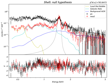
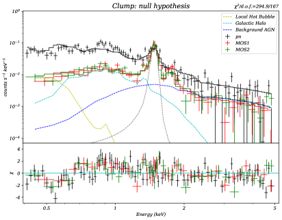
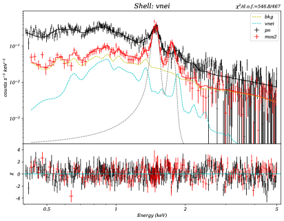
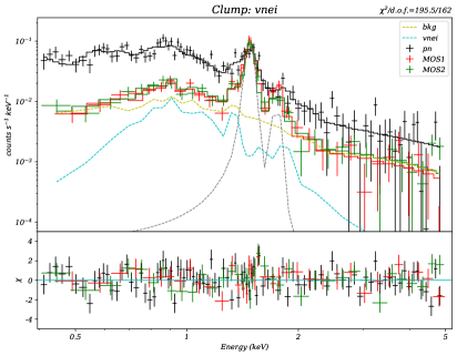
Figure 5: Spectra with folded models of region Shell (left column) and Clump (right column). From top to bottom are null hypothesis, vnei, vpshock, vapec, and vapec* models. Different components of the MOS2 spectra are labeled with dashed lines. The null hypothesis spectra mark the astrophysical background from the local hot bubble, galactic halo, and background in yellow, cyan, and blue, respectively. For the others, the astrophysical background is labeled in yellow while the extra thermal component is marked in cyan. Grey lines represent the Al-K fluorescence lines of the instrument background.

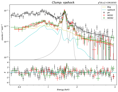
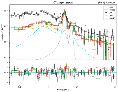
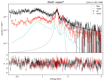
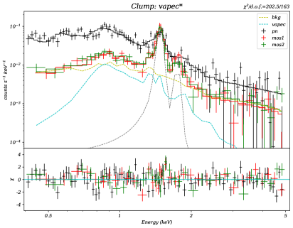
Figure 5: Continued.

Appendix C Significance of diffuse emission

Here we verify the significance of diffuse emission quantitatively mainly based on the following two methods. Firstly, the F-test is widely used to tell the significance of an extra component in spectral fittings . It would give a probability based on the chi-square and degrees of freedom of two different models, one of which has an extra component. A smaller probability (e.g. lower than $10^{-2}$ or $10^{-3}$) indicates higher significance. Besides different models describing the physical property of the diffuse emission mentioned in §3, we also test the “null hypothesis” for comparison. Assuming that the diffuse emission originates from the fluctuation, we directly use the background model to fit the source spectra, and the results are also listed in Table 1. Comparing the null hypothesis with the vnei model, the probabilities given by the F-test are $5\times 10^{-32}$ and $4\times 10^{-13}$, for Shell and Clump, respectively.

Meanwhile, we study the probability distribution of the emission measure, or rather the parameter norm in Table 1, which is proportional to the unabsorbed flux. As the parameter error is asymmetric and non-Gaussian, we use the XSPEC script steppar to fit the spectra while stepping the value of the emission measure logarithmically from $10^{-6}\,\mathrm{cm}^{-5}$ to $10^{-2}\,\mathrm{cm}^{-5}$. The chi-square increases rapidly when the emission measure drops below $\sim 10^{-5}\,\mathrm{cm}^{-5}$ and have a 5$\sigma$ lower limit around this value as plotted in Figure 6. Therefore, we conclude that the detection of the diffuse emission is robust.

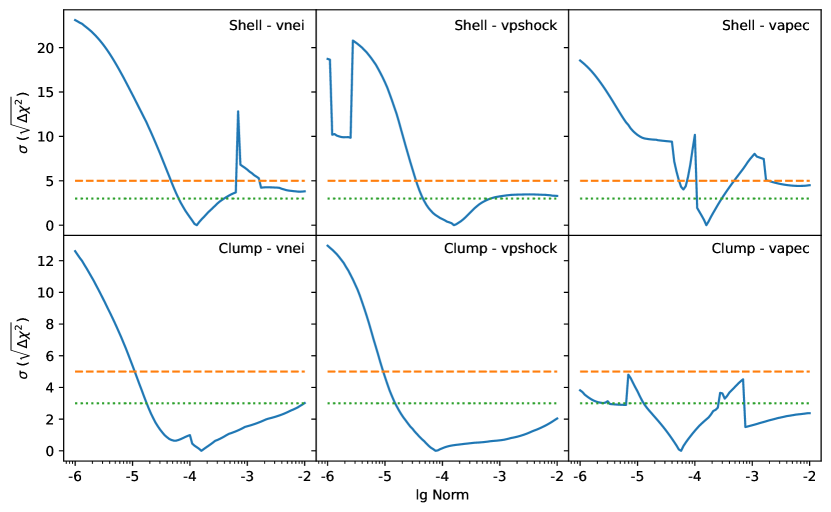
Figure 6: Relation between the change in the chi-square ($\Delta\chi^{2}$) and the value of emission measure (in units of cm^-5) given by steppar for three models in two regions (blue solid lines). Green dotted lines and orange dashed lines mark the fitting statistics corresponding to 3$\sigma$ ($\Delta\chi^{2}$=9) and 5$\sigma$ ($\Delta\chi^{2}$=25) confidence level. With large degrees of freedom, the chi-square distribution can be approximated as the Gaussian distribution.

Appendix D Supernova remnant in Sedov-Taylor phase

The physical properties of the Shell are calculated using the fitting results of NEI models. The density depends on the volume of X-ray-emitting gas and here we assume the Shell and Clump have an average depth of $\sim 5^{\prime}$ (approximately the width of the Shell region) at a distance of 5 kpc (Su et al., 2018). The region area is based on the backscal keyword of the spectra. Hence, we estimate the average density of the Shell is:

$$n=\sqrt{\frac{4\times 10^{14}\pi\,norm\,D^{2}}{1.2\eta V}}\approx(0.03\,\mathrm{cm^{-3}})\left(\frac{norm}{1.4\times 10^{-4}\,\mathrm{cm^{-5}}}\right)^{\frac{1}{2}}\left(\frac{D}{5\,\mathrm{kpc}}\right)^{-\frac{1}{2}},$$ (D1)

where $D\sim 5$ kpc is the distance of W50 (Su et al., 2018). For the Clump where X-ray emission is enhanced, its density is a little higher with $n\approx(0.05\,\mathrm{cm^{-3}})(norm/10^{-4}\,\mathrm{cm^{-5}})^{1/2}(D/5\,\mathrm{kpc})^{-1/2}$.

Noticeably, this density is much lower than that in the X-ray lobe of $\sim$1 cm^-3 95 pc away from SS 433 (Brinkmann et al., 2007; Safi-Harb et al., 2022), indicative of different gas densities in the two regions. Assuming the X-ray shell is located at the radio boundary of W50 ($28^{\prime}$ to SS 433) but projected inside the nebula, the distance of the Shell to SS 433 is obtained as:

$$R=(41\,\mathrm{pc})\,\left(\frac{D}{5\,\mathrm{kpc}}\right)$$ (D2)

and the gas mass swept by the shock $M_{s}$ (assumed in a uniform medium) is:

$$M_{s}=\frac{4}{3}\pi R^{3}\ 1.4m_{p}n_{0}=(74\,\mathrm{M_{\odot}})\left(\frac{norm}{1.4\times 10^{-4}\,\mathrm{cm^{-5}}}\right)^{\frac{1}{2}}\left(\frac{D}{5\,\mathrm{kpc}}\right)^{\frac{5}{2}},$$ (D3)

where $m_{p}$ is the proton mass and $n_{0}=n/4$ is the density of pre-shock gas. As the swept mass exceeds that of the ejecta (in general $<10$ M_⊙ (Sukhbold et al., 2016)) the SNR should have left the free expansion phase and entered the Sedov phase (Sedov, 1959; Taylor, 1950) when the SNR evolves adiabatically. The shock velocity is also typical for SNRs in the Sedov-Taylor phase, but larger than that in the radiative phase ($\lesssim 200$ km s^-1, Vink, 2020).

With the temperature of the plasma, we can derive the shock velocity:

$$v_{s}=\sqrt{\frac{16kT}{3\mu m_{p}}}=(923\,\mathrm{km\,s^{-1}})\,\left(\frac{kT}{1\,\mathrm{keV}}\right)^{\frac{1}{2}}$$ (D4)

where $\mu=0.6$ is the mean atomic weight for fully ionized plasma. Assuming a uniform ambient ISM, the age of W50 is

$$t=\frac{2R}{5v_{s}}=(17.4\,\mathrm{kyr})\,\left(\frac{D}{5\,\mathrm{kpc}}\right)\left(\frac{kT}{1\,\mathrm{keV}}\right)^{-\frac{1}{2}}.$$ (D5)

With age in Equation D5, we can calculate the expected ionization timescale of the hot gas and compare it with the X-ray spectral fitting results:

$$\tau=n_{e}t=(2.0\times 10^{10}\,\mathrm{s\,cm^{-3}})\left(\frac{norm}{1.4\times 10^{-4}\,\mathrm{cm^{-5}}}\right)^{\frac{1}{2}}\left(\frac{D}{5\,\mathrm{kpc}}\right)^{\frac{1}{2}}\left(\frac{kT}{1\,\mathrm{keV}}\right)^{-\frac{1}{2}},$$ (D6)

which is consistent with our spectral analysis ($10^{10}-10^{11}$ s cm^-3). Then we obtained the explosion energy of

$$E_{\rm SN}=\frac{R^{5}}{\xi t^{2}}\ 1.4m_{p}n_{0}=(9.3\times 10^{50}\,\mathrm{erg})\,\left(\frac{norm}{1.4\times 10^{-4}\,\mathrm{cm^{-5}}}\right)^{\frac{1}{2}}\left(\frac{D}{5\,\mathrm{kpc}}\right)^{\frac{5}{2}}\left(\frac{kT}{1\,\mathrm{keV}}\right),$$ (D7)

where dimension-less factor $\xi=2.025$. This is a typical value for a core-collapse SN (Vink, 2020).

As a high-mass X-ray binary, SS 433 should have a massive progenitor system, which can drive strong stellar winds to create a large, low-density wind-blown bubble. If the SNR is evolving in a circumstellar medium with a density $n\propto r^{-2}$ (r is the distance to the central star), the age is derived as $t=\frac{2R}{3v_{s}}\approx 28.6$ kyr (Vink, 2020), higher than in uniform medium but in the same order. In the wind bubble scenario, the dimension-less factor in Equation D7 can be expressed approximately by Truelove & McKee (1999):

$$\xi=\frac{(5-s)(10-3s)}{8\pi},$$ (D8)

where $s=2$ for a wind bubble. Applying it along with the age of 28.6 kyr as mentioned above to the Equation D7, the explosion energy would be $\sim 1.4\times 10^{51}$ erg, $\sim 1.5$ times that in a uniform environment. It should be noted that even adopting the fitting results of the CIE model shown in Table 1, the age (Equation D5) and explosion energy (Equation D7) do not change significantly. Moreover, the expected ionization timescale (Equation D6) is still $\lesssim 10^{11}$ s cm^-3, not reaching CIE yet.

Another factor that needs considering is that the heating timescale of electrons can be longer than the age of an SNR (see Borkowski et al., 2001; Ghavamian et al., 2013, and references therein) but in Equation D4 the electrons and ions are assumed with the same temperature. Here we use the measured ionization timescale $\tau$, although with higher uncertainties compared to the temperature, to recalculate the age in Equation D5:

$$t=\frac{\tau}{n_{e}}=(26.4\mathrm{\,kyr})\,\left(\frac{\tau}{3\times 10^{10}\,\mathrm{s\,cm^{-3}}}\right)\left(\frac{norm}{1.4\times 10^{-4}\,\mathrm{cm^{-5}}}\right)^{-\frac{1}{2}}\left(\frac{D}{5\,\mathrm{kpc}}\right)^{\frac{1}{2}}$$ (D9)

and the explosion energy in Equation D7:

$$E_{\mathrm{SN}}=(4.0\times 10^{50}\mathrm{\,erg})\,\left(\frac{norm}{1.4\times 10^{-4}\,\mathrm{cm^{-5}}}\right)^{\frac{3}{2}}\left(\frac{D}{5\,\mathrm{kpc}}\right)^{\frac{7}{2}}\left(\frac{\tau}{3\times 10^{10}\,\mathrm{s\,cm^{-3}}}\right)^{-2}.$$ (D10)

This explosion energy is slightly lower than that given in Equation D7 but is also reasonable for a core-collapse SNR.

It should be noted that the age and explosion energy here are based on strong assumptions and have uncertainty. Besides the fitting errors in Table 1, the real spatial structure of X-ray-emitting gas is unknown. Meanwhile, the evolution model is based on isotropic explosion and uniform density distribution, while asymmetric explosion may happen for core-collapse SNRs (e.g., Lopez et al., 2011), and current data reveal the density gradients. Anyhow, the calculation here is still representative, indicating that a black hole could form with a canonical SN.

Appendix E Equatorial Disk Wind

The equatorial disk wind may also blow out a bubble. For SS 433, the disk wind velocity has been measured based on independent optical and radio observations for the regions with a polar angle $\alpha>$ 60°. The wind velocity is $\sim 1300$ km s^-1 and $\sim 100$ km s^-1 when $\alpha$ is 60° and 90° respectively, while an average value is $\sim 450$ km s^-1 (Fabrika, 2004; Waisberg et al., 2019). The mass transfer rate as the function of polar angle is unclear, but the total mass loss rate is $10^{-4}$ M_⊙ yr^-1 (van den Heuvel, 1981; Shkovskii, 1981; Fuchs et al., 2006) and it grows as the polar angle $\alpha$ increases (Fabrika, 2004). For simplicity, we assume the wind is isotropic with a mass loss rate of $\dot{M}_{w}=10^{-4}$ M_⊙ yr^-1 and a wind velocity of $v_{w}=1000$ km s^-1, which is around the upper limit of the average wind velocity. Assuming a constant wind, the power of the wind is:

$$L_{w}=\frac{1}{2}\dot{M}_{w}v_{w}^{2}=3\times 10^{37}\,\mathrm{erg\,s^{-1}}.$$ (E1)

To compare with the SNR scenario, we also calculate the “average power” of the SN by simply dividing the explosion energy by the age:

$$L_{SN}=\frac{E_{\rm SN}}{t}=(1.7\times 10^{39}\,\mathrm{erg\,s^{-1}})\,\left(\frac{norm}{1.4\times 10^{-4}\,\mathrm{cm^{-5}}}\right)^{\frac{1}{2}}\left(\frac{D}{5\,\mathrm{kpc}}\right)^{\frac{3}{2}}\left(\frac{kT}{1\,\mathrm{keV}}\right)^{\frac{3}{2}},$$ (E2)

which is significantly higher than the power of equatorial disk wind.

Thus, the disk wind is far from a powerful energy source. For a better illustration, we applied a toy evolution model of a wind bubble based on the self-similar solution (Weaver et al., 1977; Mac Low & McCray, 1988). The radius of the bubble $R$ can be expressed as:

$$R=(10.6\,\mathrm{pc})\left(\frac{L_{37}t_{5}^{3}}{n_{0}}\right)^{1/5},$$ (E3)

where $L_{37}$, $t_{5}$, and $n_{0}$ are the wind power, bubble age, and ambient density in units of $10^{37}$ erg s^-1, $10^{5}$ yr, and 1 cm^-3, respectively. In a wind bubble, the temperature decreases from the center to the edge:

$$kT=(0.39\,\mathrm{keV})L_{37}^{8/35}n_{0}^{2/35}t_{5}^{-6/35}(1-x)^{2/5},$$ (E4)

where $x=\frac{r}{R}$ is the dimensionless distance as the ratio of the distance from the bubble center $r$ to the bubble radius $R$. Its mean value of the whole bubble is:

$$k\bar{T}=(0.21\,\mathrm{keV})L_{37}^{8/35}n_{0}^{2/35}t_{5}^{-6/35}.$$ (E5)

With this equation and Equation E3, we can get a relation among the bubble size, temperature, and wind power independent of its age and ambient gas:

$$k\bar{T}=(0.19\,\mathrm{keV})\left(\frac{L_{w}}{3\times 10^{37}\,\mathrm{erg\,s^{-1}}}\right)^{2/7}\left(\frac{R}{40\mathrm{\,pc}}\right)^{-2/7}.$$ (E6)

Therefore, if the disk wind contributes to the diffuse X-ray emission, the temperature would be significantly lower than the 3$\sigma$ lower limit (0.71 keV for vnei and 0.55 keV for vpshock) according to spectral analysis of the northern X-ray shell. The index $\frac{2}{7}$ suggests the temperature is not sensitive to the size of W50 and the wind power.

We use the moving-mesh hydrodynamical software Arepo (Springel, 2010) to simulate the evolution of the wind-blown bubble and the collision between the isotropic disk wind and a dense cloud 40 pc north of SS 433. The simulation box size is 150 pc$\times$150 pc$\times$150 pc. We initially set $5.2\times 10^{5}$ Voronoi cells, placing a 10-M_⊙ black hole particle in the center of the simulation box. The number density of the dense cloud is defined by a spherically symmetric Gaussian distribution. The maximum density is set to 120 cm^-3 and its 3$\sigma$ radial size is $15^{\prime}$, corresponding to a total mass of 25,000 M_⊙ given by Li et al. (2020). Besides the initial dense cloud, we set a uniform density background of 0.01 cm^-3 inferred from our X-ray spectral analysis. The dense cloud and the homogeneous diffuse gas have a uniform initial gas temperature of $10^{4}$ K.

In every time step of our simulation, we find 32 cells closest to the central black hole and add the corresponding mass, momentum, and kinetic energy of the disk wind to the cells, weighted by the cell solid angles extended to the central point. We include the self-gravity of the gas and multiple cooling mechanisms, which contain thermal bremsstrahlung, hydrogen and helium recombination, and solar-abundance metal line cooling (Li et al., 2019). However, we emphasize that neither self-gravity nor cooling plays an important role in our simulation.

The simulation is applied until the age of the system reaches 224 kyr. We firstly let the cloud on the plane perpendicular to the line of sight to better display the number density $n$ and temperature $T$ distributions of the wind bubble in the simulation snapshots. Then, as the X-ray emission looks inside the radio shell (Figure 2) probably due to the projection effect, we also integrate the surface brightness in a direction where the perpendicular distance from the cloud to the central black hole is 30 pc. To estimate the X-ray emission intensity, we use Xspec to calculate the absorbed X-ray emissivity (unit: erg s^-1 cm^-3) of plasma with a given temperature from 0.1 to 3.0 keV. The foreground column density is set to $7\times 10^{21}$ cm² based on the spectral analysis above. By integrating the emissivity along the line of sight, we can estimate the surface brightness (unit: erg s^-1 deg^-2) of the bubble in 0.4–2.5 keV. The snapshots of the gas number density, gas temperature, and surface brightness map of our simulation are shown in Figure 3.

Here, we compare the surface brightness (in a unit of  erg s^-1 deg^-2) between the simulation and observation. We obtained the surface brightness of $1.1\times 10^{35}$ erg s^-1 deg^-2 and $6.1\times 10^{35}$ erg s^-1 deg^-2 for the Shell and the Clump, respectively. During the whole evolution, the surface brightness of the bubble shell is always more than 1 order of magnitude lower than that of the Shell. For the Clump, we select an elliptical region with a major axis of 12 pc and a minor axis of 6 pc (the same size as the region for spectral analysis) and plot the evolution of its average surface brightness in Figure 7(a). This light curve reaches a peak near 90 kyr when the cloud begins to be shocked by the wind. Even the peak surface brightness only reaches half of that of the Clump.

The comparison of the gas temperature is less straightforward since the X-ray emission of our simulation comes from multi-temperature plasma but the spectral analysis is based on a single-temperature model. In Figure 7(b)(c)(d), we show the normalized X-ray luminosity as a function of the gas temperature for the whole wind-blown bubble at the ages of 20, 90, and 150 kyr. The mean temperature is 0.60, 0.52, and 0.56 keV, respectively, less than that given by the observation. At 20 kyr, the X-ray emission is completely from the shell as the shock has not arrived at the cloud. At 90 and 150 kyr, the X-rays are dominated by the Clump.

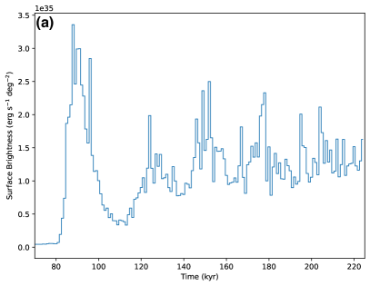
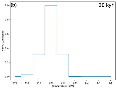
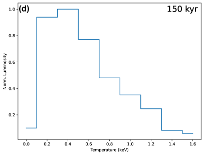
Figure 7: (a): Average surface brightness evolution of the wind bubble in the region Clump. (b)(c)(d): Normalized luminosity distribution of the temperature in 20, 90, and 150 kyr, respectively. At 20 kyr, the X-ray emission is completely from the shell as the shock has not arrived at the cloud. At 90 and 150 kyr, the X-rays are dominated by the clump. The last bin (1.6 keV) represents the temperature range above 1.5 keV.

Appendix F Image of TeV $\gamma$-ray emission

Here we compare the spatial distribution of X-ray $\gamma$-ray emission in different bands in Figure 8. We applied H.E.S.S. (Aharonian et al., 2006) data in the TeV band with relatively good spatial resolution (H. E. S. S. Collaboration et al., 2024). To extend the other energy regimes, we also plot associated $\gamma$-ray sources detected previously with the Fermi-LAT (Atwood et al., 2009) data (0.02-300 GeV, Li et al., 2020) and LHAASO WCDA (1-25 TeV) and KM2A ($>25$ TeV) data (Cao et al., 2023).

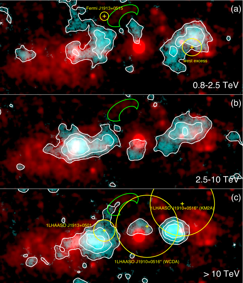
Figure 8: Spatial relations between X-rays and $\gamma$-rays. The dual-band image consists of ROSAT X-ray images of W50 (red) and the significance of H.E.S.S. data in the 0.8–2.5 ((a)), 2.5–10 ((b)), and $>10$ TeV ((c)) bands (H. E. S. S. Collaboration et al., 2024) (cyan). The white contours show the 1.5$\sigma$, 3$\sigma$, and 4.5$\sigma$ confidence level of the TeV emission. The X-ray image is in square root scale and the contour levels are 1.5, 3.0, and 4.5$\sigma$. The newly discovered X-ray shell is labeled in green. In the upper panel, the yellow crosses mark the location of GeV source Fermi J1913+0515 and the “west excess” (Li et al., 2020) and the circle stands for the position uncertainty. In the lower panel, the yellow crosses labels LHAASO source 1LHAASO J1913+0515 (detected by KM2A) and 1LHAASO J1910+0516* (detected by WCDA and KM2A)(Cao et al., 2023), with the circles the 1$\sigma$ extension or 95% extension upper limit of the sources.

References

- Abeysekara et al. (2018) Abeysekara, A. U., Albert, A., Alfaro, R., et al. 2018, Nature, 562, 82, doi: 10.1038/s41586-018-0565-5
- Aharonian et al. (2006) Aharonian, F., Akhperjanian, A. G., Bazer-Bachi, A. R., et al. 2006, A&A, 457, 899, doi: 10.1051/0004-6361:20065351
- Arnaud (1996) Arnaud, K. A. 1996, in Astronomical Society of the Pacific Conference Series, Vol. 101, Astronomical Data Analysis Software and Systems V, ed. G. H. Jacoby & J. Barnes, 17
- Atwood et al. (2009) Atwood, W. B., Abdo, A. A., Ackermann, M., et al. 2009, ApJ, 697, 1071, doi: 10.1088/0004-637X/697/2/1071
- Borkowski et al. (2001) Borkowski, K. J., Lyerly, W. J., & Reynolds, S. P. 2001, ApJ, 548, 820, doi: 10.1086/319011
- Boumis et al. (2007) Boumis, P., Meaburn, J., Alikakos, J., et al. 2007, MNRAS, 381, 308, doi: 10.1111/j.1365-2966.2007.12276.x
- Bowler (2018) Bowler, M. G. 2018, A&A, 619, L4, doi: 10.1051/0004-6361/201834121
- Brinkmann et al. (2005) Brinkmann, W., Kotani, T., & Kawai, N. 2005, A&A, 431, 575, doi: 10.1051/0004-6361:20041768
- Brinkmann et al. (2007) Brinkmann, W., Pratt, G. W., Rohr, S., Kawai, N., & Burwitz, V. 2007, A&A, 463, 611, doi: 10.1051/0004-6361:20065570
- Cao et al. (2023) Cao, Z., Aharonian, F., An, Q., et al. 2023, arXiv e-prints, arXiv:2305.17030, doi: 10.48550/arXiv.2305.17030
- Cappellari & Copin (2003) Cappellari, M., & Copin, Y. 2003, MNRAS, 342, 345, doi: 10.1046/j.1365-8711.2003.06541.x
- Chen et al. (1997) Chen, L. W., Fabian, A. C., & Gendreau, K. C. 1997, MNRAS, 285, 449, doi: 10.1093/mnras/285.3.449
- Cherepashchuk et al. (2019) Cherepashchuk, A. M., Postnov, K. A., & Belinski, A. A. 2019, MNRAS, 485, 2638, doi: 10.1093/mnras/stz610
- Churazov et al. (2024) Churazov, E. M., Khabibullin, I. I., & Bykov, A. M. 2024, arXiv e-prints, arXiv:2401.14770, doi: 10.48550/arXiv.2401.14770
- Diehl & Statler (2006) Diehl, S., & Statler, T. S. 2006, MNRAS, 368, 497, doi: 10.1111/j.1365-2966.2006.10125.x
- Dubner & Giacani (2015) Dubner, G., & Giacani, E. 2015, A&A Rev., 23, 3, doi: 10.1007/s00159-015-0083-5
- Dubner et al. (1998) Dubner, G. M., Holdaway, M., Goss, W. M., & Mirabel, I. F. 1998, AJ, 116, 1842, doi: 10.1086/300537
- Fabrika (2004) Fabrika, S. 2004, Astrophys. Space Phys. Res., 12, 1, doi: 10.48550/arXiv.astro-ph/0603390
- Fabrika (1997) Fabrika, S. N. 1997, Ap&SS, 252, 439, doi: 10.1023/A:1000885810366
- Fang et al. (2020) Fang, K., Charles, E., & Blandford, R. D. 2020, ApJ, 889, L5, doi: 10.3847/2041-8213/ab62b8
- Farnes et al. (2017) Farnes, J. S., Gaensler, B. M., Purcell, C., et al. 2017, MNRAS, 467, 4777, doi: 10.1093/mnras/stx338
- Fruscione et al. (2006) Fruscione, A., McDowell, J. C., Allen, G. E., et al. 2006, in Society of Photo-Optical Instrumentation Engineers (SPIE) Conference Series, Vol. 6270, Society of Photo-Optical Instrumentation Engineers (SPIE) Conference Series, ed. D. R. Silva & R. E. Doxsey, 62701V, doi: 10.1117/12.671760
- Fryer et al. (2018) Fryer, C. L., Andrews, S., Even, W., Heger, A., & Safi-Harb, S. 2018, ApJ, 856, 63, doi: 10.3847/1538-4357/aaaf6f
- Fuchs et al. (2006) Fuchs, Y., Koch Miramond, L., & Ábrahám, P. 2006, A&A, 445, 1041, doi: 10.1051/0004-6361:20042160
- Gabriel et al. (2004) Gabriel, C., Denby, M., Fyfe, D. J., et al. 2004, in Astronomical Society of the Pacific Conference Series, Vol. 314, Astronomical Data Analysis Software and Systems (ADASS) XIII, ed. F. Ochsenbein, M. G. Allen, & D. Egret, 759
- Gao et al. (2011) Gao, X. Y., Han, J. L., Reich, W., et al. 2011, A&A, 529, A159, doi: 10.1051/0004-6361/201016311
- Ghavamian et al. (2013) Ghavamian, P., Schwartz, S. J., Mitchell, J., Masters, A., & Laming, J. M. 2013, Space Sci. Rev., 178, 633, doi: 10.1007/s11214-013-9999-0
- Gies et al. (2002) Gies, D. R., Huang, W., & McSwain, M. V. 2002, ApJ, 578, L67, doi: 10.1086/344436
- Goodall et al. (2011) Goodall, P. T., Alouani-Bibi, F., & Blundell, K. M. 2011, MNRAS, 414, 2838, doi: 10.1111/j.1365-2966.2011.18388.x
- H. E. S. S. Collaboration et al. (2024) H. E. S. S. Collaboration, Olivera-Nieto, L., Reville, B., Hinton, J., & Tsirou, M. 2024, Science, 383, 402, doi: 10.1126/science.adi2048
- Han & Li (2020) Han, Q., & Li, X.-D. 2020, ApJ, 896, 34, doi: 10.3847/1538-4357/ab8d3d
- Jansen et al. (2001) Jansen, F., Lumb, D., Altieri, B., et al. 2001, A&A, 365, L1, doi: 10.1051/0004-6361:20000036
- Kaaret et al. (2023) Kaaret, P., Ferrazzoli, R., Silvestri, S., et al. 2023, arXiv e-prints, 2311.16313, doi: 10.48550/arXiv.2311.16313
- Kochanek (2014) Kochanek, C. S. 2014, ApJ, 785, 28, doi: 10.1088/0004-637X/785/1/28
- Kuntz & Snowden (2008) Kuntz, K. D., & Snowden, S. L. 2008, A&A, 478, 575, doi: 10.1051/0004-6361:20077912
- Li et al. (2019) Li, H., Vogelsberger, M., Marinacci, F., & Gnedin, O. Y. 2019, MNRAS, 487, 364, doi: 10.1093/mnras/stz1271
- Li et al. (2020) Li, J., Torres, D. F., Liu, R.-Y., et al. 2020, Nature Astronomy, 4, 1177, doi: 10.1038/s41550-020-1164-6
- Li (2003) Li, X.-D. 2003, ApJ, 596, L199, doi: 10.1086/379624
- Li (2007) —. 2007, ApJ, 666, L81, doi: 10.1086/521791
- Lockman et al. (2007) Lockman, F. J., Blundell, K. M., & Goss, W. M. 2007, MNRAS, 381, 881, doi: 10.1111/j.1365-2966.2007.12170.x
- Lopez et al. (2011) Lopez, L. A., Ramirez-Ruiz, E., Huppenkothen, D., Badenes, C., & Pooley, D. A. 2011, ApJ, 732, 114, doi: 10.1088/0004-637X/732/2/114
- Mac Low & McCray (1988) Mac Low, M.-M., & McCray, R. 1988, ApJ, 324, 776, doi: 10.1086/165936
- Medvedev et al. (2018) Medvedev, P. S., Khabibullin, I. I., Sazonov, S. Y., Churazov, E. M., & Tsygankov, S. S. 2018, Astronomy Letters, 44, 390, doi: 10.1134/S1063773718060038
- Mineshige et al. (1997) Mineshige, S., Nomura, H., Hirose, M., Nomoto, K., & Suzuki, T. 1997, ApJ, 489, 227, doi: 10.1086/304776
- Nomoto & Hashimoto (1988) Nomoto, K., & Hashimoto, M. 1988, Phys. Rep., 163, 13, doi: 10.1016/0370-1573(88)90032-4
- Nomoto et al. (2013) Nomoto, K., Kobayashi, C., & Tominaga, N. 2013, ARA&A, 51, 457, doi: 10.1146/annurev-astro-082812-140956
- Panferov (2017) Panferov, A. A. 2017, A&A, 599, A77, doi: 10.1051/0004-6361/201629256
- Paragi et al. (1999) Paragi, Z., Vermeulen, R. C., Fejes, I., et al. 1999, A&A, 348, 910, doi: 10.48550/arXiv.astro-ph/9907169
- Peek et al. (2018) Peek, J. E. G., Babler, B. L., Zheng, Y., et al. 2018, ApJS, 234, 2, doi: 10.3847/1538-4365/aa91d3
- Protassov et al. (2002) Protassov, R., van Dyk, D. A., Connors, A., Kashyap, V. L., & Siemiginowska, A. 2002, ApJ, 571, 545–559, doi: 10.1086/339856
- Safi-Harb & Ögelman (1997) Safi-Harb, S., & Ögelman, H. 1997, ApJ, 483, 868, doi: 10.1086/304274
- Safi-Harb & Petre (1999) Safi-Harb, S., & Petre, R. 1999, ApJ, 512, 784, doi: 10.1086/306803
- Safi-Harb et al. (2022) Safi-Harb, S., Mac Intyre, B., Zhang, S., et al. 2022, ApJ, 935, 163, doi: 10.3847/1538-4357/ac7c05
- Sedov (1959) Sedov, L. I. 1959, Similarity and Dimensional Methods in Mechanics
- Shakura & Sunyaev (1973) Shakura, N. I., & Sunyaev, R. A. 1973, A&A, 24, 337
- Shkovskii (1981) Shkovskii, I. S. 1981, Soviet Ast., 25, 315
- Smith et al. (2001) Smith, R. K., Brickhouse, N. S., Liedahl, D. A., & Raymond, J. C. 2001, ApJ, 556, L91, doi: 10.1086/322992
- Snowden et al. (2004) Snowden, S. L., Collier, M. R., & Kuntz, K. D. 2004, ApJ, 610, 1182, doi: 10.1086/421841
- Springel (2010) Springel, V. 2010, MNRAS, 401, 791, doi: 10.1111/j.1365-2966.2009.15715.x
- Strüder et al. (2001) Strüder, L., Briel, U., Dennerl, K., et al. 2001, A&A, 365, L18, doi: 10.1051/0004-6361:20000066
- Su et al. (2018) Su, Y., Zhou, X., Yang, J., et al. 2018, ApJ, 863, 103, doi: 10.3847/1538-4357/aad04e
- Sukhbold et al. (2016) Sukhbold, T., Ertl, T., Woosley, S. E., Brown, J. M., & Janka, H. T. 2016, ApJ, 821, 38, doi: 10.3847/0004-637X/821/1/38
- Sukhbold & Woosley (2014) Sukhbold, T., & Woosley, S. E. 2014, ApJ, 783, 10, doi: 10.1088/0004-637X/783/1/10
- Taylor (1950) Taylor, G. 1950, Proceedings of the Royal Society of London Series A, 201, 159, doi: 10.1098/rspa.1950.0049
- Truelove & McKee (1999) Truelove, J. K., & McKee, C. F. 1999, ApJS, 120, 299, doi: 10.1086/313176
- Truemper (1982) Truemper, J. 1982, Advances in Space Research, 2, 241, doi: 10.1016/0273-1177(82)90070-9
- Turner et al. (2001) Turner, M. J. L., Abbey, A., Arnaud, M., et al. 2001, A&A, 365, L27, doi: 10.1051/0004-6361:20000087
- van den Heuvel (1981) van den Heuvel, E. P. J. 1981, Vistas in Astronomy, 25, 95, doi: 10.1016/0083-6656(81)90050-7
- Vink (2020) Vink, J. 2020, Physics and Evolution of Supernova Remnants (Springer Cham), doi: 10.1007/978-3-030-55231-2
- Waisberg et al. (2019) Waisberg, I., Dexter, J., Petrucci, P.-O., Dubus, G., & Perraut, K. 2019, A&A, 623, A47, doi: 10.1051/0004-6361/201834746
- Wang et al. (2006) Wang, Z., Chakrabarty, D., & Kaplan, D. L. 2006, Nature, 440, 772, doi: 10.1038/nature04669
- Weaver et al. (1977) Weaver, R., McCray, R., Castor, J., Shapiro, P., & Moore, R. 1977, ApJ, 218, 377, doi: 10.1086/155692
- Wilms et al. (2000) Wilms, J., Allen, A., & McCray, R. 2000, ApJ, 542, 914, doi: 10.1086/317016
- Woosley & Heger (2007) Woosley, S. E., & Heger, A. 2007, Phys. Rep., 442, 269, doi: 10.1016/j.physrep.2007.02.009
- Woosley & Heger (2015) —. 2015, ApJ, 810, 34, doi: 10.1088/0004-637X/810/1/34
- Woosley et al. (2002) Woosley, S. E., Heger, A., & Weaver, T. A. 2002, Reviews of Modern Physics, 74, 1015, doi: 10.1103/RevModPhys.74.1015
- Zealey et al. (1980) Zealey, W. J., Dopita, M. A., & Malin, D. F. 1980, MNRAS, 192, 731, doi: 10.1093/mnras/192.4.731
- Zhang et al. (2008) Zhang, W., Woosley, S. E., & Heger, A. 2008, ApJ, 679, 639, doi: 10.1086/526404