Principle and prospect of Bose-Einstein correlation study at BESIII

Abstract

One method to determine the characteristic parameters of a hadron production source is to measure Bose-Einstein correlation functions. In this paper, we present fundamental concepts and formulas related to Bose-Einstein correlations, focusing on the measurement principles and the Lund model from an experimental perspective. We perform Monte Carlo simulations using the Lund model generator in the 2–3 GeV energy range. Through these feasibility studies, we identify key features of Bose-Einstein correlations that offer valuable insights for experimental measurements. Utilizing data samples collected at BESIII, we propose measurements of Bose-Einstein correlation functions, with the expected experimental precision of the hadron source radius and incoherence parameter at the level of a few percent.

I Introduction

The hadron production process in electron-positron collisions is described as $e^{+}$ and $e^{-}$ annihilate into a virtual photon ($\gamma^{\ast}$), which splits into an initial quark-antiquark pair ($q\bar{q}$). The hadronization process consists of three phases: (1) perturbative Quantum Chromodynamics (pQCD) cascade evolutions of quarks and gluons; (2) hadron source formation and preliminary hadrons emission; and (3) the decay of unstable hadrons.

In the energy region of the Beijing Electron Positron Collider II (BEPCII), which ranges from 2 to 5 GeV, the preliminary hadron states include continuous states and resonant states characterized by the quantum numbers $J^{PC}=1^{--}$. Since the hadronization process cannot be predicted comprehensively and quantitatively by pQCD, phenomenological models are used to describe this phase. One of the commonly used model is the semi-classical Lund string fragmentation model lundmodel ; bohu . The Lund model describes the hadron source as a string, which fragments into hadrons.

The production of vector resonant states such as $\rho$, $\omega$, $\phi$, $J/\psi$, $\psi(3686)$, can be summarized as follows: the $\gamma^{\ast}$ evolves into $q\bar{q}$ pair, which constitutes the vector meson. The meson then decays into final states, a process explained by the vector meson dominance model ioffe .

In quantum mechanics, the propagation of hadrons can be described using wave functions. The wave function of a system of identical bosons is symmetric under the interchange of the space-time coordinates of any two bosons. This symmetry results in a higher probability of finding identical bosons in a small phase-space element than different bosons, as illustrated in Fig.1. This phenomenon is known as Bose-Einstein correlation (BEC), which is independent of specific interactions. Measurements of the BEC effect provide valuable space-time information about the hadron source boal ; weiner .

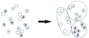
Figure 1: Identical bosons in hadron final states are more likely reassigning in closer phase space.

Theoretical studies of the BEC effect have been conducted for many years, leading to various assumptions about the space-time distribution of the hadron source, including Gaussian-type, ellipsoid-type boal ; weiner , and more generalized L$\acute{e}$vy-distribution phenix ; adare ; csorgo .

Experimental measurements of the BEC effect have been carried out in $e^{+}e^{-}$, $p\bar{p}$ collisions, $ep$ and $Kp$ scattering to select various signal samples at energies ranging from tens of GeV to TeV, as performed by numerous collaborations. Some of these are listed in Table I, with more detailed experiments documented in Ref.boutemeur . All these experiments demonstrate the universal characteristics of the BEC effect.

Collaboration	Beam	$\sqrt{s}$(GeV)	Boson-pairs
MARKII markii	$e^{+}e^{-}$	29	$\pi^{\pm}\pi^{\pm}$
AMY amy	$e^{+}e^{-}$	58	$\pi^{\pm}\pi^{\pm}$
OPAL opal	$e^{+}e^{-}$	91	$\pi^{\pm}\pi^{\pm}$, $\pi^{0}\pi^{0}$
L3 l3 ; achard	$e^{+}e^{-}$	91	$\pi^{0}\pi^{0}$
NA22 na22	$\pi^{+}p$,$K^{+}p$	21.7	$\pi^{\pm}\pi^{\pm}$
ZEUS epzeus	ep	10.5	$\pi^{\pm}\pi^{\pm}$,$K^{\pm}K^{\pm}$
CMS cms	pp	900,2360	$\pi^{\pm}\pi^{\pm}$
ATLAS atlas	pp	13000	$\pi^{\pm}\pi^{\pm}$
ALICE alice	pp	900,7000	$\pi^{+}\pi^{+}$
PHENIX phenix	AuAu	200	$\pi^{\pm}\pi^{\pm}$

Table I. Status of measurements of BEC effect.

However, in the BEPCII energy region, measurements of the BEC effect are still lacking. The BESIII detector at BEPCII has collected data samples with large statistics at certain energies, providing the opportunity to measure the BEC effect. In this paper, we first introduce the basic concepts of the BEC effect and derive the emission amplitude of the hadron source based on the Lund model, along with the wave functions of a two-pion system. We then perform feasibility studies using the Monte Carlo (MC) method by the Lund model generator to explore some properties relevant to measuring the BEC effect.

II Hadron source in Lund model

II.1 Hadron production at space-time point

The hadron source in the Lund model is not static, and it evolves in space-time according to the Lund area law bohu . Hadrons are emitted from convex vertices at various space-time points by string fragmentation. The mass and momentum of a hadron originate from the potential energy stored in the string. Figure 2 shows that meson $i$ is produced at space-time point $i=(x_{i},t_{i})$, composed of $q_{A}$ and $\bar{q}_{B}$ located at adjacent concave vertices A=$(x_{A},t_{A})$ and B=$(x_{B},t_{B})$. The mass and energy-momentum of meson $i$ satisfy relativistic mass-energy relation lundmodel :

$$\frac{E_{i}^{2}-p_{i}^{2}}{\kappa^{2}}=\frac{m_{i}^{2}}{\kappa^{2}}=(x_{A}-x_{B})^{2}-(t_{A}-t_{B})^{2},$$ (1)

where $\kappa$ is the attractive tension constant between quark and antiquark.

Equation (1) indicates that points A and B lie on two hyperbolas, and the space-time interval between A and B cannot be too small to ensure that the produced hadron has the required mass. Consequently, the hadron source in the Lund model is discontinuous in space-time.

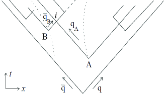
Figure 2: Meson $i$ with constituent quarks $q_{A}$ and $\bar{q}_{B}$ lie on hyperbolas of space-time.

The Lund area law provides a strict solution for the Lund model. The probability of producing $n$ hadrons is given by lundmodel ; bohu :

$$d{\cal P}_{n}(\{p_{j}\})=\delta^{2}(P_{n}-\sum_{j=1}^{n}p_{j})\prod_{j=1}^{n}d^{2}p_{j}\delta(p_{j}^{2}-m_{j}^{2})|{\cal M}_{n}|^{2},$$ (2)

where $p_{j}$ is the momentum component of the hadron parallel to the string, and $m_{j}$ is the transverse mass. The matrix element ${\cal M}_{n}$ is expressed as:

$${\cal M}_{n}=\exp[i\xi{\cal A}_{n}],~{}~{}\xi=1/2\kappa+ib/2$$ (3)

where ${\cal A}_{n}$ is the light-cone area, and $b$ is a dynamics constant.

The space-time $\{x_{i}\}$ and energy-momentum $\{p_{i}\}$ are related through Eq.(1), implying that these sets of quantities are equivalent. Thus, ${\cal M}_{n}$ can be viewed as a function of either $\{x_{i}\}$ or $\{p_{i}\}$ equivalently:

$${\cal M}_{n}={\cal M}_{n}(\{p_{i}\};\{x_{i}\})~{}~{}{\rm or}~{}~{}{\cal M}_{n}={\cal M}_{n}(\{x_{i}\};\{p_{i}\}),$$ (4)

where the quantities in the first braces are the variables of ${\cal M}_{n}$, and those in the second braces are the conjugate parameters. In principle, using the correspondence between $\{x_{i}\}$ and $\{p_{i}\}$ and the Jacobian transformation, $d{\cal P}_{n}(\{p_{j}\})$ in Eq.(2) can be rewritten as the conjugate expression $d{\cal P}_{n}(\{x_{j}\})$ in space-time coordinates, which is the space-time distribution of hadron emitting source.

II.2 Emitting amplitude of hadron source

To match experimental data, the Lund model incorporates phenomenological parameters that represent hadron production ratios at each vertex jetset ; bohu . Consequently, each matrix element ${\cal M}_{n}$ is associated with a set of additional parameters dependent on the hadron type, denoted as the factor $g_{n}$. The exclusive hadron emitting amplitude $F_{n}(\{x_{i}\};\{p_{i}\})$ can be expressed as:

$$F_{n}(\{x_{i}\};\{p_{i}\})\sim g_{n}{\cal M}_{n}(\{x_{i}\};\{p_{i}\}).$$ (5)

The emitting amplitude of a single particle produced at $x_{i}$ and with momentum $p_{i}$ in an event of multiplicity $n$ can be written as:

$$f_{n}(x_{i};p_{i})\sim\sum_{j\not=i}F_{n}(\{x_{j}\};\{p_{j}\}),$$ (6)

which is a complex number and depends on the hadron category.

The quantity $f_{n}(x_{i};p_{i})$ described in Eq.(6) is impossible to calculate analytically. The single-particle emitting probability amplitude is obtained from MC samples with a fixed multiplicity $n$ numerically:

$$f_{n}(x_{i};p_{i})\sim\frac{1}{N_{evt}}\sum_{ievt}^{Nevt}\sum_{j\not=i}F_{n}(\{x_{j}\};\{p_{j}\}),$$ (7)

where $N_{evt}$ is the number of events in the MC sample. The inclusive single hadron emitting probability amplitude in MC simulations corresponds to:

$$f(x_{i};p_{i})\sim\frac{1}{N_{evt}}\sum_{ievt}^{Nevt}\sum_{n}\sum_{j\not=i}F_{n}(\{x_{j}\};\{p_{j}\}).$$ (8)

III Wave function of two-pion system

In relativistic expression, a free and stable particle is described by a plane wave function (strictly speaking, the motion of particles should be described by wave packets):

$$\psi(x;p)\sim\exp(ipx).$$ (9)

For certain hadrons, such as $\pi^{\pm}$ and $K^{\pm}$, their lifetime are sufficiently long to be considered stable in experiments. And for an unstable particle with short life-time (resonance), the wave function can be written as:

$$\psi(x;p)\sim\frac{m\Gamma}{s-m^{2}+im\Gamma}\exp(ipx),$$ (10)

where $m$ is the peak position of resonance (the mass of resonance), $s$ is the square of the center-of-mass energy, $\Gamma$ is the decay width, this indicates the lifetime of particle $\tau=\hbar/\Gamma$. For simplicity, we neglect the phase factor $\exp(i\theta)$ as it does not affect the analysis of the BEC effect.

However, if a particle is influenced by Coulomb and strong interactions, the corresponding wave function becomes significantly more complex hepph9606365 . This study does not discuss the situation of final state interaction.

For BESIII detector, the space coordinate origin $O$ is set at the center of the detector, which also serves as the collision point of $e^{+}e^{-}$, and the time origin is synchronized with the event trigger clock of the data acquisition system.

As shown in Fig.3, two pions ($\pi^{+}\pi^{-}$ and $\pi^{\pm}\pi^{\pm}$) are emitted from the hadron source points at $x_{i}=({\bf r_{i}},t_{i})$ and $x_{j}=({\bf r_{j}},t_{j})$ respectively, and are detected by detectors Da at $x_{a}=({\bf r_{a}},t_{a})$ and Db at $x_{b}=({\bf r_{b}},t_{b})$. Here, ${\it\bf r}_{a}$ and ${\it\bf r}_{b}$ are the central positions of Da and Db relative to $O$, and $t_{a}$ and $t_{b}$ represent the times of particles traveling from $O$ to Da and Db.

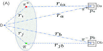
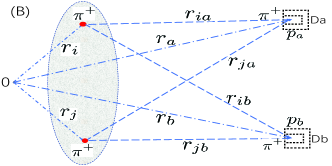
Figure 3: $\pi^{+}\pi^{-}$ and $\pi^{+}\pi^{+}$ are emitted from hadron source and detected by detectors Da and Db.

For a real detector, Da is not a point but has a finite range, and time and momentum are measured with uncertainties, so the detected interval $x_{ia}$ and $p_{a}$ can be expressed as:

$$x_{ia}=x_{a}-x_{i}+\delta x_{ia}~{}~{}{\rm and}~{}~{}p_{a}=p_{i}+\delta p_{a},$$ (11)

where $\delta x_{ia}$ and $\delta p_{a}$ reflect the detected space-time and energy-momentum uncertainties. The wave function of $\pi^{+}$ arriving at $x_{a}$ is given by:

$$\psi(i;a) \equiv \psi(x_{ia};p_{a})=\exp(ip_{a}x_{ia})$$ (12)

$$= \exp(ip_{a}x_{a})\times\exp(-ip_{a}x_{i}+i\delta_{ia}),$$

where $\delta_{ia}=p_{a}\delta x_{ia}+\delta p_{a}x_{ia}$ is a random phase angle, possibly with observable effects on the measurement of correlation functions.

Similarly, the wave function of $\pi^{-}$ emitted from $x_{j}$ with momentum $p_{j}$ and detected by Db at $x_{b}$ with momentum $p_{b}$ is:

$$\psi(j;b) \equiv \psi(x_{jb};p_{b})=\exp(ip_{b}x_{jb})$$ (13)

$$= \exp(ip_{b}x_{b})\times\exp(-ip_{b}x_{j}+i\delta_{jb}),$$

where $x_{jb}=x_{b}-x_{j}+\delta x_{jb}$, $p_{b}=p_{j}+\delta p_{b}$, and $\delta_{jb}=p_{b}\delta x_{jb}+\delta p_{b}x_{jb}$.

The joint wave function of $\pi^{+}\pi^{-}$ arriving at Da and Db is:

$$\psi_{d}(i,j;a,b)\equiv\psi(i,a)\psi(j,b)=\psi(x_{ia};p_{a})\psi(x_{jb};p_{b}).$$ (14)

This expression $\psi_{d}$ also is applicable for $\pi^{\pm}\pi^{0}$.

As depicted in Fig.3(B), $\pi^{+}$ and $\pi^{+}$ are detected by Da and Db with momenta $p_{a}$ and $p_{b}$ respectively. The two identical pions are indistinguishable in measurement, meaning Da and Db cannot determine whether a $\pi^{+}$ was emitted from $x_{i}$ or $x_{j}$. Consequently, the joint wave function of $\pi^{+}\pi^{+}$ has a symmetrized form for interchanging source points $i$ and $j$:

$$\psi_{s}(i,j;a,b)\equiv\frac{1}{\sqrt{2}}[\psi(i;a)\psi(j;b)+\psi(j;a)\psi(i;b)].$$ (15)

The expression $\psi_{s}$ also applicable for $\pi^{-}\pi^{-}$ and $\pi^{0}\pi^{0}$.

If the preliminary state contains unstable particles that decay into stable final states, due to the fact that the lifetimes of most unstable particles are only a few femtometer (much smaller than the spatial resolution of the detector), the decay vertex is considered as part of the uncertainty in the emitting position in experiments.

IV Detection probability amplitudes

The inclusive detection probability amplitudes for $\pi^{+}$ and $\pi^{-}$, emitted from points $x_{i}$ and $x_{j}$ and detected by detectors Da and Db with momenta $p_{a}$ and $p_{b}$, are expressed as follows:

$${\cal A}(i;a)\equiv{\cal A}(x_{ia};p_{a})=f(x_{i};p_{i})\psi(x_{ia};p_{a}),$$ (16)

$${\cal A}(j;b)\equiv{\cal A}(x_{jb};p_{b})=f(x_{j};p_{j})\psi(x_{jb};p_{b}).$$ (17)

In these calculations, we assume $p_{a}=p_{i}$ and $p_{b}=p_{j}$, incorporating measurement uncertainties into the random phase angles $\delta_{ia}$ and $\delta_{jb}$, and they can be absorbed into the functions $f(x_{i};p_{a})$ and $f(x_{j};p_{b})$, respectively. Therefore, the detection probability amplitudes not only encode information about the hadron sources but are also influenced by measurement uncertainties.

The joint probability amplitude for detecting $\pi^{+}$ and $\pi^{-}$ by Da and Db is given by:

$${\cal A}_{d}(i,j;a,b)\equiv{\cal A}(i;a){\cal A}(j;b).$$ (18)

For the case where two identical $\pi^{+}\pi^{+}$ are detected by Da and Db, there are four probability amplitudes, as shown in Fig.3(B). Besides the two already given by Eqs.(16) and (17), the additional amplitudes are:

$$~{}~{}{\cal A}(j,a)\equiv{\cal A}(x_{ja};p_{a})=f(x_{j};p_{j})\psi(x_{ja};p_{a}),$$ (19)

$${\cal A}(i,b)\equiv{\cal A}(x_{ib};p_{b})=f(x_{i};p_{i})\psi(x_{ib};p_{b}),$$ (20)

The joint probability amplitude for detecting $\pi^{+}\pi^{+}$ is then:

$${\cal A}_{s}(i,j;a,b)\equiv\frac{1}{\sqrt{2}}[{\cal A}(i,a){\cal A}(j,b)+{\cal A}(j,a){\cal A}(i,b)],$$ (21)

which is symmetric with respect to the interchange of source points $i$ and $j$.

V Correlation function of two pions

The expression of the correlation function for a two-pion system varies depending on whether the measurement is coherent or incoherent.

V.1 Coherent and incoherent measurements

One of the key considerations in BEC effect measurements is determining whether the measurement is coherent or incoherent. These two types of measurements are represented by different formulas, leading to different results. In other words, the results of the measurement are influenced not only by the detected particles but also by the measurement method and the status of the detector. A more detailed explanation of how to distinguish between coherent and incoherent measurements can be found in Ref.boal .

The principles determining whether a measurement of BEC effect is coherent or incoherent are analogous to those in the well-known electron double-slit experiments. If the experiment does not detect through which slit the electron passes, the screen will display interference (coherent) patterns. Conversely, if the electron’s path is detected, the screen will show non-interferential (incoherent) patterns. Similar results have been observed in double-slit experiments using neutrons and atoms, indicating the universal quantum characteristics of microscopic particles.

Based on the principles found in double-slit experiments, we can define the criteria for a BEC measurement to be coherent or incoherent as follows:

$\bullet$ Incoherent measurement: If the detector can determine the emission position and the trajectory of a particle, such as with the BESIII detector shown in Fig.4(A), using a vertex detector (VD) or track reconstruction in the main drift chamber (MDC), the measurement is considered incoherent. In this scenario, the detection of particle paths eliminates interference effects.

$\bullet$ Coherent measurement: If the detector is such that it cannot determine the emission position and trajectory, like the setup shown in Fig.4(B), where the VD and MDC are turned off and only the electromagnetic calorimeter (EMC) is operational, the measurement is considered coherent. In this case, the inability to track the particle paths allows interference patterns to emerge.

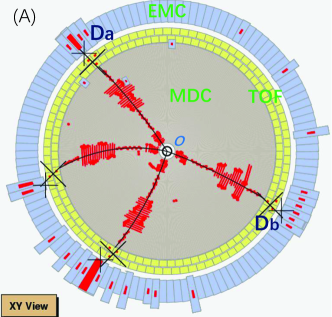
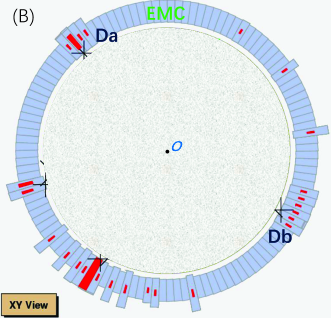
Figure 4: Sketch figures of two kinds of detectors. Detector (A) can determine where the particle emitting from, but detector (B) can not.

For a real detector that falls somewhere between the status of Fig.4(A) and Fig.4(B), the detected correlation functions should be a combination of both incoherent and coherent terms. This mixed measurement results from partial information about particle trajectories, leading to partial interference effects.

V.2 Incoherent correlation distributions

When measurements are performed using data collected with an ideal and perfect detector as shown in Fig.4(A), the measurement is guaranteed to be incoherent. This incoherence is a consequence of the inherent quantum characteristics of the system.

$\bullet$ Single pion distribution: When a hadron source emits a pion from position $x_{i}$ with momentum $p_{i}$, and it is detected by detector Da with momentum $p_{a}$, the inclusive probability distribution is given by:

$$P_{1}^{I}(p_{a})=\sum_{i}|{\cal A}(i;a)|^{2}=\sum_{i}|f(x_{i};p_{a})|^{2},$$ (22)

which depends on the space-time distribution of hadron source only.

$\bullet$ Two different pions distribution: For a pair of $\pi^{+}\pi^{-}$ emitted from positions $x_{i}$ with momentum $p_{i}$ and $x_{j}$ with momentum $p_{j}$, and detected by Da with momentum $p_{a}$ and Db with momentum $p_{b}$, the incoherent correlation distribution is:

$$P_{2d}^{I}(p_{a},p_{b}) = \sum_{i,j}|{\cal A}_{d}(i,j;a,b)|^{2}$$ (23)

$$= P_{1}^{I}(p_{a})P_{1}^{I}(p_{b})=P_{2}^{I}(p_{a},p_{b}).$$

This equation shows that the incoherent correlation distribution for different pion types is the product of individual single-pion probability distributions. The same expression also applies to pairs of $\pi^{\pm}\pi^{0}$.

$\bullet$ Two identical pions distribution: For a pair of $\pi^{+}\pi^{+}$, emitted from positions $x_{i}$ with momentum $p_{i}$ and $x_{j}$ with momentum $p_{j}$, and detected by Da with momentum $p_{a}$ and Db with momentum $p_{b}$, the incoherent correlation distribution is:

$$P_{2s}^{I}(p_{a},p_{b}) = \frac{1}{2}\sum_{i,j}|{\cal A}_{s}(i,j;a,b)|^{2}$$ (24)

$$= P_{2}^{I}(p_{a},p_{b})+P_{s}^{I}(p_{a},p_{b}),$$

where the additional term is defined as:

$$P_{s}^{I}(p_{a},p_{b})=\sum_{i,j}{\cal A}^{\ast}(i;a){\cal A}^{\ast}(j;b){\cal A}(i;b){\cal A}(j;a).$$ (25)

In Eq.(24), the first term represents the genuine incoherent correlation distribution, similar to $P_{2d}^{I}(p_{a},p_{b})$ in Eq.(23). The second term, $P_{s}^{I}(p_{a},p_{b})$, is the interference, which accounts for phase averaging between the detection amplitudes of the two $\pi^{+}$ in ${\cal A}_{s}$ given by Eq.(21). The interference term $P_{s}^{I}(p_{a},p_{b})$ in Eq.(25) disappears if the phases $\{\delta_{ia}\}$ and $\{\delta_{jb}\}$ in wave functions Eq.(12) and Eq.(13) fluctuate randomly. The same expressions also apply to pairs of $\pi^{-}\pi^{-}$ and $\pi^{0}\pi^{0}$.

V.3 Coherent correlation distributions

When data samples are collected using the detector as shown in Fig.4(B), the measurements are coherent.

$\bullet$ Single particle distribution: The inclusive distribution of a pion emitted from $x_{i}$ with momentum $p_{i}$ and detected by Da with momentum $p_{a}$ is given by:

$$P_{1}^{C}(p_{a}) = |\sum_{i}{\cal A}(i;a)|^{2}$$ (26)

$$= P_{1}^{I}(p_{a})+\sum_{i\not=j}{\cal A}^{\ast}(i;a){\cal A}(j;a).$$

In this expression, the first term $P_{1}^{I}(p_{a})$, as given by Eq.(22), represents the incoherent contribution, which depends on the intensity of individual sources, and the second term is the coherent contribution, reflecting interference between different source points. In the summation of these cross terms, each amplitude has a corresponding conjugate term, and their imaginary parts cancel each other out, leaving only the real parts.

$\bullet$ Two different pions correlation: For a pair of $\pi^{+}$ and $\pi^{-}$ detected by Da with momentum $p_{a}$ and by Db with momentum $p_{b}$ respectively, the coherent correlation distribution is:

$$P_{2d}^{C}(p_{a},p_{b}) = |\sum_{i,j}{\cal A}(i;a){\cal A}(j;b)|^{2}$$ (27)

$$= P_{2}^{I}(p_{a},p_{b})+P_{d}^{C}(p_{a},p_{b}),$$

where

$$P_{d}^{C}(p_{a},p_{b})=\sum_{i\not=k,j\not=l}{\cal A}^{\ast}(i;a){\cal A}^{\ast}(j;b){\cal A}(k;a){\cal A}(l;b).$$ (28)

In Eq.(27), the first term is the incoherent correlation function given by Eq.(23), and the second term, $P_{d}^{C}(p_{a},p_{b})$, is the true coherent one.

$\bullet$ Two identical pions correlation: For a pair of identical $\pi^{+}\pi^{+}$ detected by Da and Db with momentum $p_{a}$ and $p_{b}$ respectively, the coherent correlation distribution is:

$$P_{2s}^{C}(p_{a},p_{b}) = |\sum_{i,j}{\cal A}_{s}(i,j;a,b)|^{2}$$

$$= P_{2}^{I}(p_{a},p_{b})+P_{s}^{I}(p_{a},p_{b})+P_{s}^{C}(p_{a},p_{b}),$$

where $P_{s}^{I}(p_{a},p_{b})$ is given by Eq.(25), and

$$P_{s}^{C}(p_{a},p_{b})=\sum_{i\not=k,j\not=l}{\cal A}^{\ast}(k;a){\cal A}(l;a){\cal A}^{\ast}(j;b){\cal A}(l;b)$$ (30)

is true coherent term of the symmetric wave function. The sign (positive or negative) of the summation of cross terms is determined by the average of the random phases in Eqs.(12) and (13). This inherently quantum property leads to the measurement results being experiment-dependent due to the random phase angles caused by experimental uncertainties.

Many factors contribute to correlation effects in the hadron final state. For instance, the $\delta$ function in Eq.(2) imposes strong restrictions on hadron distribution, leading to energy-momentum correlations among all final state particles. The correlation effect caused by energy-momentum conservation depends on the topology of event multiplicity. To avoid bias, both the signal sample and the reference sample should be selected from events with the same multiplicity.

V.4 Correlation function reflecting BEC effect

Now, we focus exclusively on the BEC effect. The BEC function (BECF) in experiments is defined as the ratio of the correlation functions of identical bosons (signal sample) to the correlation functions of different bosons (reference sample). This ratio isolates the BEC effect by counteracting other correlation effects.

In an ideal scenario, if data samples of $\pi^{+}\pi^{+}$ and $\pi^{+}\pi^{-}$ are collected using a perfect detector, as depicted in Fig.4(A), this is termed an ideal measurement, because the precise information of the hadron source is detected. The ratio of their incoherent correlation functions, based on Eqs.(23) and (24), is given by:

$$C_{2}^{I}(p_{a},p_{b})=\frac{P_{2s}^{I}(p_{a},p_{b})}{P_{2d}^{I}(p_{a},p_{b})}=1+R_{2}^{I}(p_{a},p_{b}),$$ (31)

where,

$$R_{2}^{I}(p_{a},p_{b})=\frac{P_{s}^{I}(p_{a},p_{b})}{P_{d}^{I}(p_{a},p_{b})}.$$ (32)

In a more realistic scenario, if data samples of $\pi^{+}\pi^{+}$ and $\pi^{+}\pi^{-}$ are collected using an imperfect detector, as shown in Fig.4(B), this is termed a non-ideal measurement because no information about the hadron emission source is detected. In this case, the measurement is coherent, and the ratio of their correlation functions, based on Eqs.(27) and (V.3), is:

$$C_{2}^{C}(p_{a},p_{b})=\frac{P_{2s}^{C}(p_{a},p_{b})}{P_{2d}^{C}(p_{a},p_{b})}=1+R_{2}^{C}(p_{a},p_{b}),$$ (33)

where,

$$R_{2}^{C}(p_{a},p_{b})=\frac{P_{s}^{C}(p_{a},p_{b})}{P_{d}^{C}(p_{a},p_{b})}.$$ (34)

Ideally, the data collected by the detector shown in Fig.4(A) would be used to measure the BECF. However, real detectors are imperfect, often due to factors like electromagnetic noises in the Main Drift Chamber (MDC) or incomplete reconstruction of particle tracks, which means that not all emitting points of hadron source are detected. Thus, the measured BECF is:

$$C_{2}(p_{a},p_{b})=\frac{P_{2s}(p_{a},p_{b})}{P_{2d}(p_{a},p_{b})},$$ (35)

where $P_{2s}(p_{a},p_{b})$ and $P_{2d}(p_{a},p_{b})$ are combinations of incoherent and coherent correlation functions of signal samples and reference samples respectively:

$$P_{2s}(p_{a},p_{b})=P_{2s}^{I}(p_{a},p_{b})+\alpha P_{2s}^{C}(p_{a},p_{b}),$$ (36)

$$P_{2d}(p_{a},p_{b})=P_{2d}^{I}(p_{a},p_{b})+\beta P_{2d}^{C}(p_{a},p_{b}).$$ (37)

The quantities $\alpha$ and $\beta$ reflect the degree of imperfection in the detector, which causes some of hadron emissions to be measured in a coherent-like manner. Typically, $\alpha$ and $\beta$ are small, and the first-order approximation is:

$$C_{2}(p_{a},p_{b})=1+\lambda^{CI}R_{2}^{I}(p_{a},p_{b}),$$ (38)

where $R_{2}^{I}(p_{a},p_{b})$ is the ideal two-pion correlation function defined in Eq.(32), and

$$\lambda^{CI}=1+\alpha R_{2s}^{CI}(p_{a},p_{b})-\beta R_{2d}^{CI}(p_{a},p_{b}),$$ (39)

with

$$R_{2s}^{CI}(p_{a},p_{b})=\frac{P_{2s}^{C}(p_{a},p_{b})}{P_{2s}^{I}(p_{a},p_{b})},$$ (40)

$$R_{2d}^{CI}(p_{a},p_{b})=\frac{P_{2d}^{C}(p_{a},p_{b})}{P_{2d}^{I}(p_{a},p_{b})}.$$ (41)

Here, $\lambda^{CI}$ represents the deviation of the measured BECF from the ideal BECF due to the real detector’s imperfections. It is noticed that this coefficient $\lambda^{CI}$ is distinct from the incoherent parameter $\lambda$ in phenomenological hadron source models and adopted in fitting of experiment data, which arises from different factors boal .

Currently, there are two main approaches to describing the origin of the BEC effect: the wave function approach and the more general field theory approach. The wave function approach is intuitive for explaining the BEC effect, making it clear that the BECF can appear coherent or incoherent depending solely on the measurement method and experimental equipment, without reference to the coherence of the hadron source. In contrast, the field theory approach assumes that the hadron source is divided into incoherent and coherent field components boal ; weiner ; csorgo .

VI BEC effect in Lund model

The BEC effect is a natural consequence of the Lund model lundmodel ; npb5131998627 . In this model, there can be multiple string configurations that fragment into the same hadron state. For example, as shown in Fig.14.1 of Ref.lundmodel , there are two configurations with light-cone areas ${\cal A}_{12}$ and ${\cal A}_{21}$, both of which fragment into the same hadron final state but with different momentums. In these configurations, two identical bosons are produced at convex vertices 1 and 2. The difference between these two configurations is simply the exchange of the two identical bosons. The total matrix element for this hadron state can be expressed as:

$${\cal M}={\cal M}_{12}+{\cal M}_{21}$$ (42)

leading to

$$|{\cal M}|^{2}=[\exp(-b{\cal A}_{12}+\exp(-b{\cal A}_{21})](1+{\cal H}).$$ (43)

Here, the term ${\cal H}$ is defined as:

$${\cal H}=\frac{\cos(\Delta{\cal A}/\kappa)}{\cosh(b\Delta{\cal A}/2)},$$ (44)

where $\Delta{\cal A}$ is the difference between ${\cal A}_{12}$ and ${\cal A}_{21}$. This shows that the interference between the two configurations ${\cal A}_{12}$ and ${\cal A}_{21}$ results in an enhancement factor of $1+{\cal H}$, This factor increases as $\Delta{\cal A}$ decreases, which occurs when the momenta $p_{1}$ and $p_{2}$ of the two identical bosons become closer to each other.

VII BECF in experimental measurement

In quantum field theory, the distribution functions are related to the differential cross-sections. For the inclusive process $a+b\to c+X$, (where $X$ represents all other particles except $c$), the differential cross-section is defined as:

$$d\sigma(p)=\frac{\sigma_{tot}}{<n>}\tilde{\rho}_{1}(p)d\phi=\sigma_{tot}\rho_{1}(p)d\phi,$$ (45)

where $d\phi$ is the phase-space element of particle $c$, $<n>$ is the average multiplicity, and $\rho_{1}(p)$ is the single-particle density distribution. Similarly, for the two-particle differential cross section in process $a+b\to c_{1}+d_{2}+X$, we have

$$d^{2}\sigma(p_{1},p_{1})=\sigma_{tot}\rho_{2}(p_{1},p_{2})d\phi_{1}d\phi_{2},$$ (46)

where $\rho_{2}(p_{1},p_{2})$ is the two particle density distributions.

The relationships between the dimensionless probability distributions and the density distributions are given by:

$$P_{1}(p)\propto\rho_{1}(p)\\$$

$$P_{2}(p_{1},p_{2})\propto\rho_{2}(p_{1},p_{2}).$$ (47)

In theoretical and model studies, the correlation function often uses the following ratio:

$$R_{2}(p_{1},p_{2})=\frac{\rho_{2}(p_{1},p_{2})}{\rho_{1}(p_{1})\rho_{1}(p_{2})},$$ (48)

which is a 6-dimensional representation. However, it is more convenient to use the 1-dimensional two-particle correlation function:

$$C_{2}(Q)=1+\frac{P_{2}(Q)}{P_{11}(Q)},$$ (49)

where $Q^{2}$ is defined as the invariant squared difference of four-momenta of the two particles:

$$Q^{2}=-(p_{1}-p_{2})^{2}=(p_{1}+p_{2})^{2}-4m_{\pi}^{2}>0.$$ (50)

The correlation functions are obtained by the integrals:

$$P_{11}(Q)=\int d\phi_{1}d\phi_{2}\delta[Q^{2}+(p_{1}-p_{2})^{2}]\rho_{1}(p_{1})\rho_{1}(p_{2})$$ (51)

$$P_{2}(Q)=\int d\phi_{1}d\phi_{2}\delta[Q^{2}+(p_{1}-p_{2})^{2}][\rho_{2}(p_{1},p_{2})-\rho_{1}(p_{1})\rho_{1}(p_{2})],$$ (52)

where the pseudo correlation in $\rho_{2}(p_{1},p_{2})$ is deducted.

In experimental studies, BECFs are often parameterized as:

$${\bullet~{}\rm Exponential~{}form}~{}~{}~{}C(Q)=1+\lambda\exp(-RQ),~{}~{}$$ (53)

$${\bullet~{}\rm Gaussian~{}form}~{}~{}~{}C(Q)=1+\lambda\exp[-(RQ)^{2}],~{}~{}$$ (54)

where $\lambda$ is known as the incoherent or chaotic parameter, and $R$ is often interpreted as the source radius boal ; weiner . The line-shapes of Eqs.(53) and (54) are shown in Fig.5. In which $\lambda=0.75$ and $R=0.4$ fm are used, while the actual values are expected to be determined from fitting experimental data. From Eqs. (53) and (54), two important features of the correlation function are that it goes to $1$ at large $Q$ values, and goes to $1+\lambda$ at $Q=0$.

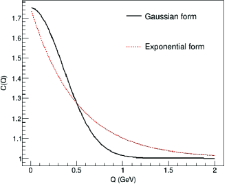
Figure 5: Line-shapes of exponential and Gaussian forms.

It is important to note that, since $Q^{2}$ is defined as a four-dimensional form in Eq.(50), the parameter $R$ in Eq.(53) and Eq.(54) does not necessarily reflect the true spatial scale of the hadron source. Instead, it also depends on the lifetime of the hadron source. Various models attempt to provide a physical explanation for parameter $\lambda$ weiner ; boal ; bolz ; csorgo . While $\lambda$ may have multiple physical factors, the term expressed in Eq.(39) is certainly a component of them.

VIII Correction factors in measurement

To fit the line shape of BECF measured by experimental data, one uses following correlation density:

$$\rho(Q_{i})=K\frac{\Delta n(Q_{i})}{\Delta Q_{i}},$$ (55)

where $\Delta n(Q_{i})$ is the number of particle pairs falling within the interval $(Q_{i},Q_{i}+\Delta Q_{i})$, and $K$ is a normalization factor.

The observed density correlation functions are obtained by selecting signal and reference particle pairs from experimental data. Some preliminary hadrons are unstable and decay into final-state hadrons before reaching the detector. The correlation functions obtained from the decay final-state hadrons are:

$$\rho_{\rm finsig}^{\rm datobs}(Q) = K_{\rm finsig}^{\rm datobs}\frac{\Delta n_{\rm finsig}^{\rm datobs}(Q)}{\Delta Q},$$ (56)

$$\rho_{\rm finref}^{\rm datobs}(Q) = K_{\rm finref}^{\rm datobs}\frac{\Delta n_{\rm finref}^{\rm datobs}(Q)}{\Delta Q},$$ (57)

the final state BECF is defined as:

$$C_{\rm fin}^{\rm datobs}(Q)=\frac{\rho_{\rm finsig}^{\rm datobs}(Q)}{\rho_{\rm finref}^{\rm datobs}(Q)}.$$ (58)

Ideally, BECF should be measured using preliminary-state hadrons. If we can trace back the decay final states to the preliminary states, the preliminary-state density correlation functions are:

$$\rho_{\rm presig}^{\rm datobs}(Q)=K_{\rm presig}^{\rm datobs}\frac{\Delta n_{\rm presig}^{\rm datobs}(Q)}{\Delta Q},$$ (59)

$$\rho_{\rm preref}^{\rm datobs}(Q)=K_{\rm preref}^{\rm datobs}\frac{\Delta n_{\rm preref}^{\rm datobs}(Q)}{\Delta Q},$$ (60)

and the observed preliminary BECF is:

$$C_{\rm pre}^{\rm datobs}(Q)=\frac{\rho_{\rm presig}^{\rm datobs}(Q)}{\rho_{\rm preref}^{\rm datobs}(Q)}.$$ (61)

Both the BECFs expressed by Eqs.(58) and (61) are dependent on data analysis method, and the physical results take into account efficiency correction.

To derive the physical BECF, $C^{\rm phy}(Q)$, from the observed $C_{\rm pre}^{\rm datobs}(Q)$ and $C_{\rm fin}^{\rm datobs}(Q)$, two sets of corrections are required: one to account for the efficiency in the analysis-dependent quantities, and another to convert the final-state $C_{\rm fin}(Q)$ to preliminary state one $C_{\rm pre}(Q)$.

If MC simulations align well with experimental data, the following relationship holds:

$$\frac{C^{\rm phy}(Q)}{C^{obs}(Q)}=\frac{C^{\rm simgen}(Q)}{C^{\rm simobs}(Q)},$$ (62)

where,

$$C^{\rm simgen}(Q)=\frac{\rho_{\rm sig}^{\rm simgen}(Q)}{\rho_{\rm ref}^{\rm simgen}(Q)},$$ (63)

$$C^{\rm simobs}(Q)=\frac{\rho_{\rm sig}^{\rm simobs}(Q)}{\rho_{\rm ref}^{\rm simobs}(Q)}$$ (64)

are the BECFs obtained by MC simulations at generator level and detector level, respectively.

For both preliminary and final states hadron simulated at generator and detector levels, we have:

$$C_{\rm pre}^{\rm simgen}(Q)=\frac{\rho_{\rm presig}^{\rm simgen}(Q)}{\rho_{\rm preref}^{\rm simgen}(Q)},~{}C_{\rm pre}^{\rm simobs}(Q)=\frac{\rho_{\rm presig}^{\rm simobs}(Q)}{\rho_{\rm preref}^{\rm simobs}(Q)},$$ (65)

$$C_{\rm fin}^{\rm simgen}(Q)=\frac{\rho_{\rm finsig}^{\rm simgen}(Q)}{\rho_{\rm finref}^{\rm simgen}(Q)},~{}C_{\rm fin}^{\rm simobs}(Q)=\frac{\rho_{\rm finsig}^{\rm simobs}(Q)}{\rho_{\rm finref}^{\rm simobs}(Q)}.$$ (66)

The experimental physics results of BECFs can be derived from the observed values by applying efficiency corrections:

$$C_{\rm pre}^{\rm datexp}(Q)=\frac{C_{\rm pre}^{\rm datobs}(Q)}{\epsilon_{\rm pre}(Q)},C_{\rm fin}^{\rm datexp}(Q)=\frac{C_{\rm fin}^{\rm datobs}(Q)}{\epsilon_{\rm fin}(Q)},$$ (67)

where the efficiencies $\epsilon_{\rm pre}$ and $\epsilon_{\rm fin}$ are obtained though MC simulations:

$$\epsilon_{\rm pre}(Q)=\frac{C_{\rm pre}^{\rm simobs}(Q)}{C_{\rm pre}^{\rm simgen}(Q)},\epsilon_{\rm fin}(Q)=\frac{C_{\rm fin}^{\rm simobs}(Q)}{C_{\rm fin}^{\rm simgen}(Q)}.$$ (68)

The relation between the experimental raw data and physics result is:

$$C^{\rm phy}(Q)=C_{\rm pre}^{\rm datexp}(Q)=f_{\rm prefin}^{\rm simgen}(Q)\cdot C_{\rm fin}^{\rm datexp}(Q),$$ (69)

where the recover factor is:

$$f_{\rm prefin}^{\rm simgen}(Q)=\frac{C_{\rm pre}^{\rm simgen}(Q)}{C_{\rm fin}^{\rm simgen}(Q)}.$$ (70)

IX Monte Carlo simulations

The MC generators for the Lund model are LUARLW (for middle to low-energy region) bohu and JETSET (for high-energy region) jetset .

The subroutine LUBOEI in LUARLW and JETSET employs algorithms based on mean-field potential attraction between identical bosons to simulate the BEC effect. This is achieved by shifting the final-state momenta of identical bosons closer together while maintaining energy-momentum conservation within the event EurPhysJC21998165 ; plb3511995293 ; BECinMP . LUBOEI offers two options for simulating the BEC effect: the exponential form (given in Eq.(53)) and the Gaussian form (given in Eq.(54)). The analysis of BESIII data indicates that the Gaussian form agrees well with experimental data, so it is used in the following MC simulations.

In this section, we present various BECF line shapes simulated at the generator level. The signal samples typically include $\pi^{+}\pi^{+}$, $\pi^{-}\pi^{-}$ and $\pi^{0}\pi^{0}$, while the reference samples include $\pi^{+}\pi^{-}$, $\pi^{\pm}\pi^{0}$. We provide comparisons between preliminary and final states for different signal and reference samples at the generator level.

In MC simulations, we can generate either preliminary hadron states only or allow unstable hadrons to decay into final states. The inclusive line shapes of normalized density distributions $\rho_{\rm presig}^{\rm simgen}(Q)$ and $\rho_{\rm preref}^{\rm simgen}(Q)$ in Eq.(65), $\rho_{\rm finsig}^{\rm simgen}(Q)$ and $\rho_{\rm finref}^{\rm simgen}(Q)$ in Eq.(66) are shown in Fig.6. The line shapes of $\rho_{\rm presig}^{\rm simgen}(Q)$ and $\rho_{\rm finsig}^{\rm simgen}(Q)$ tend towards the low $Q$ end, which is a characteristic feature of the BEC effect.

In the reference sample, some $\pi^{+}\pi^{-}$ pairs are the decay final states of resonances such as $\rho$, $\eta$, $\eta^{\prime}$, $\omega$, $\phi$. In Fig.6(B), the convexity of $\rho_{\rm finref}^{\rm simgen}(Q)$ is due to resonant effects. We can exclude these $\pi^{+}\pi^{-}$ pairs by requiring their squared invariant mass $q^{2}=(p_{\pi^{+}}+p_{\pi^{-}})^{2}$ to lie outside the resonant peak $[(M_{R}-\Gamma)^{2},(M_{R}+\Gamma)^{2}]$. However, this requirement inevitably removes some $\pi^{+}\pi^{-}$ pairs from non-resonant states.

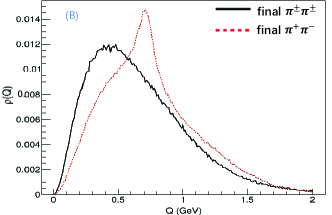
Figure 6: The density correlation function $\rho(Q)$ of preliminary state (A) and final states (B) of signal and reference samples at 3 GeV.

Various schemes for selecting reference samples have been investigated by different collaborations eurphysjc822022608 . However, these schemes can violate energy-momentum conservation. As noted in Ref.boal , the correlations arising from energy-momentum conservation are stronger than those from the BEC effect. It is expected that biases introduced by these schemes can be corrected using good MC simulations and the correction factor given in Eq.(70).

Figure 7 shows the density correlation functions $\rho(Q)$ for $\pi^{+}\pi^{-}$, $\pi^{\pm}\pi^{0}$ and $K^{+}K^{-}$ in preliminary and final states. If $\rho(Q)$ consists of only $\pi^{+}\pi^{-}$ pairs or all of $\pi^{+}\pi^{-}$, $\pi^{\pm}\pi^{0}$ and $K^{+}K^{-}$ pairs, the line shape of $C(Q)$ differs.

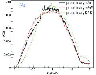
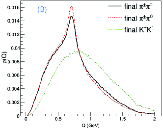
Figure 7: Density correlation function of preliminary and final states reference samples $\pi^{+}\pi^{-}$, $\pi^{\pm}\pi^{0}$ and $K^{+}K^{-}$ at 3 GeV.

Figure 8 illustrates the BECF of inclusive preliminary and final states, along with their ratio as presented by Eq.(70), indicating that the line shape of $C(Q)$ is energy-dependent within the BEPCII energy range. Figure 9 shows the dependence of BECF on preliminary and final states for semi-exclusive continuous states at 3 GeV.

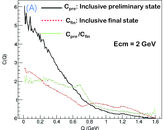
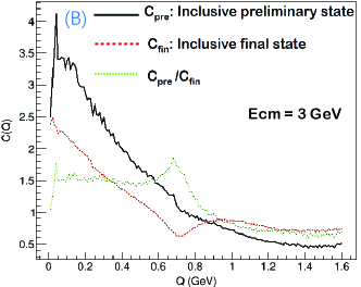
Figure 8: The BECF of inclusive preliminary and final states and their rations at 2 and 3 GeV.

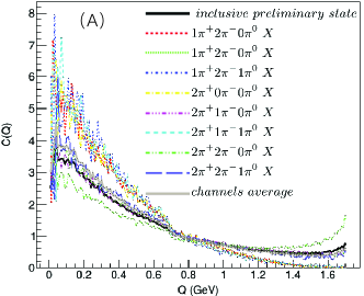
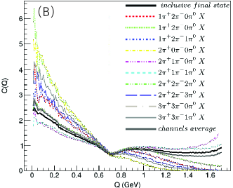
Figure 9: The BECF of semi-exclusive continuous preliminary production and final states.

The $J/\psi$ particle is produced via $e^{+}e^{-}\to\gamma^{\ast}\to c\bar{c}\to J/\psi$, and decays to preliminary states and/or stable final states. It is interesting to examine whether the BEC effect exists in the preliminary and secondary final states of $J/\psi$ decay. MC simulations reveal that both preliminary and secondary decay final states exhibit the BEC effect, as shown in Fig.10, with the line shapes of $C(Q)$ of $J/\psi$ similar to those of continuous states.

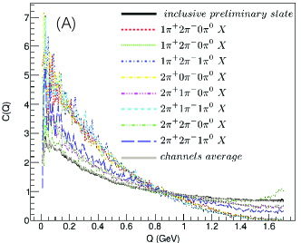
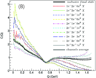
Figure 10: The BECF of semi-exclusive preliminary and secondary decay final states of 3-gluon decay mode of $J/\psi$.

The Lund model predicts that the hadron emission amplitude with a fixed multiplicity given by Eq.(7) differs from that of the inclusive case given by Eq.(8). Figure 11 shows the BECF for preliminary hadron states with $n=4,5,6$, as well as for inclusive states.

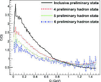
Figure 11: BECF of inclusive hadron states with different preliminary multiplicities.

Figure 12 demonstrates that the line shape of BECF depends on the choice of signal and reference samples. This implies that the BECF of the hadron source should be measured exclusively, as inclusive measurements can only capture the average features of the hadron source.

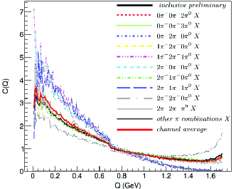
Figure 12: BECF of some semiexclusive channels, the reference sample include $\pi^{+}\pi^{-}$ and $\pi^{\pm}\pi^{0}$.

Figure 13 shows the BECF for preliminary and final states $\pi^{\pm}\pi^{\pm}$, $\pi^{0}\pi^{0}$ and $K^{\pm}K^{\pm}$, $\pi^{\pm}\pi^{\pm}$, $\pi^{0}\pi^{0}$ and $K^{\pm}K^{\pm}$, indicating that the BECF depends on the choice of signal samples.

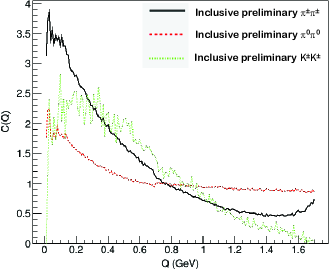
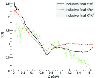
Figure 13: The BECF of preliminary and final states $\pi^{\pm}\pi^{\pm}$, $\pi^{0}\pi^{0}$ and $K^{\pm}K^{\pm}$.

It is noticed that the formulas Eqs.(53) and (54) are simplified parametric forms that describe the main characteristics of BECF. In MC simulations, LUBOEI realizes the BEC effect by the mean-field method, and the actual effects also depend on the specific hadron states. Compared with the Eqs.(53) and (54), the practical BECFs are multiplied by corresponding normalization factors, as done in most experimental data analyses opal ; na22 , and thus the actual distributions in Figs.8-13 seem different as shown in Fig.5, but the overall trends are similar.

In previous experiments, signal samples were selected using cyclic combinations, where any boson could be combined with other identical ones multiple times. This method results in non-independent $Q$ values, introducing extra correlations into $\rho(Q)$. Figure 14 shows that an event with four identical pions can have six possible cyclic combinations.

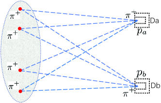
Figure 14: 4 identical $\pi$ production and detected by Da and Db.

Figure 15 illustrates the line shapes of $C(Q)$ obtained by circular and non-circular combinations of pion pairs. The former introduces extra correlation at small $Q$, which is not due to the BEC effect. The correct approach to selecting signal samples is the latter, but the number of signal identical pions is less.

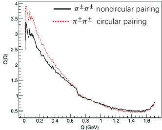
Figure 15: Comparison of BECF line-shapes between circular and noncircular combination of $\pi^{\pm}\pi^{\pm}$.

An alternative generator HYBRID hybrid is also used for the study and similar results are obtained. It combines PHOKARA phokara , CONEXC conexc and LUARLW, developed for the $R$ value measurement at BESIII besiiir .

X Summary and prospect

The semi-classical Lund string fragmentation model is currently the only phenomenological model that can present physical picture of the hadron production source and correlate the spatiotemporal distribution of the hadron source with the energy-momentum distribution of the produced hadrons.

Starting from the Lund model, we have explored some basic concepts and formulas related to the BEC effect and performed MC simulations. From these feasibility studies, several properties of the BEC effect have been identified:
(1). The Lund model establishes the relationships between the space-time points of the hadron source and the momentum of the emitted hadron.
(2). In addition to the coherent or incoherent components of the hadron source, the status of the particle detector also affects the measured values of the incoherence parameter $\lambda$ and the source scale $R$.
(3). Different choices of signal and reference samples result in different line shapes of the BECF.
(4). Experimental measurements of the BEC effect should be conducted exclusively.
(5). The space-time distribution characteristics of the hadron source are energy-dependent.
(6). We have demonstrated how to convert the observed final state BECF to that of the preliminary state one using MC simulations.

Table II presents the integrated luminosity and the number of hadron events of the data samples collected with their large statistics at BESIII, enable precise measurements of the BECF at these energies.

$E_{cm}(GeV)$	${\cal L}_{int.}~{}({\rm pb}^{-1})$	$N_{had}~{}(10^{6})$
2.125	108.5	5.89
2.396	66.9	2.85
2.645	67.8	2.35
2.900	106.0	3.06
3.080	126.0	3.09
J/$\psi$		$10^{4}$
$\psi$(2S)		3$\times 10^{3}$

Table II. Some data samples collected at BESIII.

The measurement of the BECF using the data collected at BESIII is promising. Pion pairs $\pi^{\pm}\pi^{\pm}$ and $\pi^{+}\pi^{-}$ are selected as the signal and reference samples, respectively. The generator LUARLW is used to simulate hadron production, while GEANT4 GEANT4 simulates the propagation and interaction of particles with detector materials. The primary systematic uncertainty comes from the hadron generators, for which the difference between LUARLW and HYBRID is taken as an estimation.

A preliminary analysis of BESIII data indicates that several million same-sign charged pion pairs are available at the five continuum energies. It is expected that the measurement precision for the hadron source parameters, obtained by fitting the line shape of $C(Q)$, will be better than $6\%$ for $\lambda$ and and $3\%$ for $R$. In the future, data collected at the $J/\psi$ and $\psi(2S)$ peaks will be utilized to measure the BEC effect, further enhancing our understanding of hadron source.

- (1) B. Andersson, The Lund Model, (Cambridge University Press, 1998)p. 158
- (2) B. Andersson and H. Hu, hep-ph/9910285
- (3) B.L. Ioffe et al., Hard Processes Volume 1, (Noth-Holland Physics Publising, 1984)
- (4) D.H. Boal and C.K. Gelbke, Rev. Mod. Phys. 62, 553 (1990)
- (5) R.M. Weiner, Phys. Rept. 327, 249 (2000)
- (6) T. Csrg et al., Eur. Phys. J. C 9, 275 (1999), T. Csrg et al., Eur. Phys. J. C 36, 67 (2004)
- (7) T. Novk et al., (PHENIX Collaboration), arXiv:2304.09580 [nucl-ex]
- (8) A. Adare et al., Phys. Rev. C 97, 064911 (2018)6
- (9) M. Boutemeur, Nucl. Phys. B(Proc. Suppl.) 121, 82 (2003)
- (10) I. Juricic et al., (MARKII Collaboration), Phys. Rev. D 39, 1 (1989)
- (11) S. K. Choi et al., (AMY Collaboration), Phys. Lett. B 355, 406 (1995)
- (12) G. Alexander et al., (OPAL Collaboration), Z. Phys. C 72, 389 (1996)
- (13) P. Achard et al., (L3 Collaboration), Phys. Lett. B 524, 55 (2002)
- (14) P. Achard et al., (L3 Collaboration), Eur. Phys. J. C 71, 1648 (2011)
- (15) M. Adamus et al., (EHS/NA22 Collaboration), Z. Phys. C 37, 347 (1988)
- (16) S. Checkanov et al., (ZEUS Collaboration), Phys. Lett. B 652, 1 (2007)
- (17) V. Khachatryan et al., (CMC Collaboration), Phys. Rev. Lett. 105, 032001 (2010)
- (18) G. Aad et al., (ATLAS Collaboration), Eur. Phys. C 82, 608 (2022)
- (19) K. Aamodt et al., (ALICE Collaboration), Phys. Rev. D 84, 112004 (2011)
- (20) T.Sjstrand, CERN-TH 6488/92, @5035/w5036
- (21) T. Osada et al. ArXiv:hep-ph/9606365
- (22) B. Andersson and M. Ringer, Nucl. Phys. B 513, 627 (1998)
- (23) J. Bolz et al., Phys. Rev. D 47, 3860 (1993)
- (24) L. Lnnblad, and T. Sjstrand, Phys. Lett. B 351, 293 (1995)
- (25) L. Lnnblad, and T. Sjstrand, Eur. Phys. J. C 2, 165 (1998)
- (26) T.Sjstrand, in Multiparticle Production, Eds R. Hwa, (Wold Scientific, Singapore, (1979) p.237
- (27) G. Aad et al., (ATLAS Collaboration), Eur. Phys. J. C 82, 608 (2022)
- (28) R. G. Ping et al. Chin. Phys. C 40, 113002 (2016).
- (29) H. Czyz, M. Gunia and J. H. Kuhn, JHEP08, 110 (2013)
- (30) R. G. Ping et al., Chin. Phys. C 28, 083001 (2014)
- (31) M. Ablikim et al., (BESIII Collaboration), Phys. Rev. Lett. 128, 062004 (2022)
- (32) S. Agostinelli et al., (Geant4 Collaboration), Nucl. Instrum. Meth. A 506, 250 (2003)