FedL2G: Learning to Guide Local Training in Heterogeneous Federated Learning

Abstract

Data and model heterogeneity are two core issues in Heterogeneous Federated Learning (HtFL). In scenarios with heterogeneous model architectures, aggregating model parameters becomes infeasible, leading to the use of prototypes (i.e., class representative feature vectors) for aggregation and guidance. However, they still experience a mismatch between the extra guiding objective and the client’s original local objective when aligned with global prototypes. Thus, we propose a Federated Learning-to-Guide (FedL2G ) method that adaptively learns to guide local training in a federated manner and ensures the extra guidance is beneficial to clients’ original tasks. With theoretical guarantees, FedL2G efficiently implements the learning-to-guide process using only first-order derivatives w.r.t. model parameters and achieves a non-convex convergence rate of $\mathcal{O}(1/T)$. We conduct extensive experiments on two data heterogeneity and six model heterogeneity settings using 14 heterogeneous model architectures (e.g., CNNs and ViTs) to demonstrate FedL2G’s superior performance compared to six counterparts.

1 Introduction

With the rapid development of AI techniques (Touvron et al., 2023; Achiam et al., 2023), public data has been consumed gradually, raising the need to access local data inside devices or institutions (Ye et al., 2024). However, directly using local data often raises privacy concerns (Nguyen et al., 2021). Federated Learning (FL) is a promising privacy-preserving approach that enables collaborative model training across multiple clients (devices or institutions) in a distributed manner without the need to move the actual data outside clients (Kairouz et al., 2019; Li et al., 2020). Nevertheless, data heterogeneity (Li et al., 2021; Zhang et al., 2023d; a) and model heterogeneity (Zhang et al., 2024b; Yi et al., 2023) remain two practical issues when deploying FL systems. Personalized FL (PFL) mainly focuses on the data heterogeneity issue (Zhang et al., 2023e), while Heterogeneous FL (HtFL) considers both data and model heterogeneity simultaneously (Zhang et al., 2024a). HtFL’s support for model heterogeneity enables a broader range of clients to participate in FL with their customized models.

In HtFL, sharing model parameters, a widely used technique in traditional FL and PFL, is not applicable (Zhang et al., 2024b). Instead, lightweight knowledge carriers, including small auxiliary models (Shen et al., 2020; Wu et al., 2022; Yi et al., 2024), tiny homogeneous modules (Liang et al., 2020; Yi et al., 2023), and prototypes (i.e., class representative feature vectors) (Jeong et al., 2018; Tan et al., 2022b), can be shared among clients. Of these, prototypes offer the most significant communication efficiency due to their compact size.

However, representative prototype-based methods FedDistill (Jeong et al., 2018) and FedProto (Tan et al., 2022b), still suffer from a mismatch between the prototype-guiding objective and the client’s original local objective. These methods typically introduce an extra guiding objective alongside the original local objective, aiming to guide local features to align with the global ensemble prototypes. Due to the significant variation in width and depth among clients’ heterogeneous models, their feature extraction capabilities also differ considerably (Zhang et al., 2024a; b). On the other hand, the data distribution also diverges across clients (McMahan et al., 2017; Li et al., 2022). Since the global prototypes are derived from aggregating diverse local prototypes, they inherently cannot fully align with specific client models and their respective data. Consequently, directly optimizing the guiding and local objectives together without prioritizing the original local objective has the potential to undermine the local objective of each client due to the objective mismatch. We illustrate an example of this mismatch problem in Fig. 1, where the “negative effect” is measured by the maximum increase between the current local loss and the previous lowest local loss during federated training.

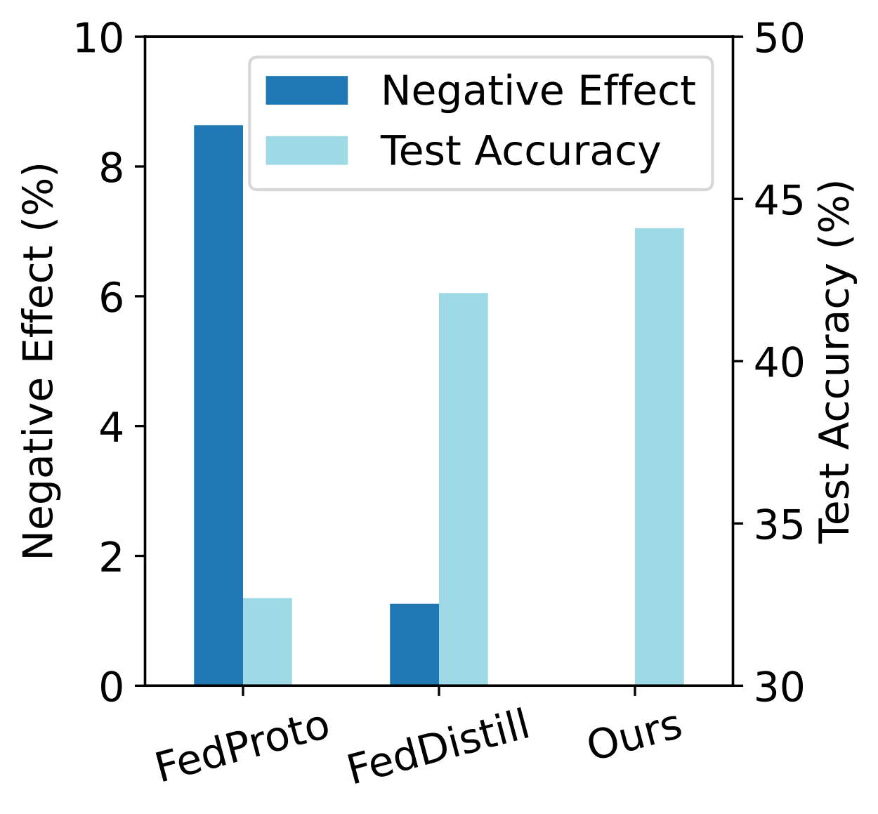
Figure 1: An example of the negative effect and test accuracy of three HtFL methods.

To address the issue of objective mismatch, we propose a novel Federated Learning-to-Guide (FedL2G) method. It gives priority to the original local objective while learning the guiding objective, ensuring that the guiding objective can facilitate each client’s original local task rather than causing negative effects. This is why we term it “learning to guide”. Specifically, we hold out a tiny quiz set from the training set and denote the remaining set as a study set on each client. Then we learn guiding vectors in a federated manner, ensuring that updating client models with both the extra guiding loss and the original local loss on their study sets consistently reduces the original local loss on their quiz sets (which are not used for training and testing). The minimal negative effect (close to zero) and the superior test accuracy illustrated in Fig. 1 embody the design philosophy and effectiveness of our FedL2G. Moreover, in contrast to learning-to-learn (Finn et al., 2017; Jiang et al., 2019; Fallah et al., 2020a), the learning-to-guide process in our FedL2G only requires first-order derivatives w.r.t. model parameters, making it computationally efficient.

We assess the performance of our FedL2G across various scenarios. In addition to test accuracy, we also evaluate communication and computation overhead. We summarize our contributions as:

• In the context of HtFL with data and model heterogeneity, we analyze and observe the objective mismatch issue between the extra guiding objective and the original local objective within representative prototype-based methods.

• We propose a FedL2G method that prioritizes the original local objective while using the extra guiding objective, thus eliminating negative effects.

• We theoretically prove that FedL2G achieves efficiency using only first-order derivatives w.r.t. model parameters, with a non-convex convergence rate of $\mathcal{O}(1/T)$.

• To demonstrate our FedL2G ’s priority, we conducted extensive experiments covering two types of data heterogeneity, six types of model heterogeneity (including 14 distinct model architectures such as CNNs and ViTs), and various system settings.

2 Related Work

2.1 Heterogeneous Federated Learning (HtFL)

Presently, FL is one of the popular collaborative learning and privacy-preserving techniques (Zhang et al., 2023d; Li et al., 2020) and HtFL extends traditional FL by supporting model heterogeneity (Ye et al., 2023). Prevailing HtFL methods primarily consider three types of model heterogeneity: (1) group heterogeneity, (2) partial heterogeneity, and (3) full heterogeneity (Zhang et al., 2024b). Among them, the HtFL methods considering group model heterogeneity extract different but architecture-constraint sub-models from a global model for different groups of clients (Diao et al., 2020; Horvath et al., 2021; Wen et al., 2022; Luo et al., 2023; Zhou et al., 2023). Thus, they cannot support customized client models and are excluded from our consideration. Additionally, sharing and revealing model architectures within each group of clients also raises privacy and intellectual property concerns (Zhang et al., 2024a). As the server is mainly utilized for parameter aggregation in prior FL systems (Tan et al., 2022a; Kairouz et al., 2019), training a server module with a large number of epochs, like (Zhang et al., 2024b; a; Zhu et al., 2021), necessitates additional upgrades or the purchase of a new heavy server, which is impractical. Thus, we focus on the server-lightweight methods.

Both partial and full model heterogeneity accommodate customized client model architectures, but partial heterogeneity still assumes some small parts of all client models to be homogeneous. For example, LG-FedAvg (Liang et al., 2020) and FedGH (Yi et al., 2023) stand out as two representative approaches. LG-FedAvg and FedGH both partition each client model into a feature extractor part and a classifier head part, operating under the assumption that all classifier heads are homogeneous. In LG-FedAvg, the parameters of classifier heads are uploaded to the server for aggregation, whereas FedGH uploads prototypes to the server and trains the lightweight global classifier head for a small number of epochs. Both methods utilize the global head for knowledge transfer among clients but overlook the inconsistency between the global head and local tasks.

In the case of full model heterogeneity, mutual distillation (Zhang et al., 2018) and prototype guidance (Tan et al., 2022b) emerge as two prevalent techniques. Using mutual distillation, FML (Shen et al., 2020) and FedKD (Wu et al., 2022) facilitate knowledge transfer among clients through a globally shared auxiliary model. However, sharing an entire model demands substantial communication resources, even if the auxiliary model is typically small (Zhang et al., 2024b). Furthermore, aggregating a global model in scenarios with data heterogeneity presents numerous challenges, such as client-drift (Karimireddy et al., 2020), ultimately leading to a subpar global model (Li et al., 2022; Zhang et al., 2023a; b; c). As representative prototype guidance methods, FedDistill (Jeong et al., 2018) and FedProto (Tan et al., 2022b) gather prototypes on each client, aggregate them on the server to create the global prototypes, and guide client local training with these global prototypes. Specifically, FedDistill extracts lower-dimensional prototypes than FedProto. This difference stems from FedDistill applying prototype guidance in the logit space, whereas FedProto uses the intermediate feature space. Sharing higher-dimensional prototypes can transfer more information among clients; however, it may also exacerbate the negative effects of objective mismatch.

2.2 Student-Centered Guidance

Our learning-to-guide philosophy draws inspiration from student-centered knowledge distillation approaches (Yang et al., 2024). They are based on the insight that a teacher’s subject matter expertise alone may not match the student’s specific studying ability and style, resulting in negative effects (Sengupta et al., 2023; Yang et al., 2024). To address the mismatch between the teacher’s knowledge and the needs of the student, updating the teacher model with concise feedback from the student on a small quiz set represents a promising direction (Ma et al., 2022; Zhou et al., 2022; Sengupta et al., 2023).

However, these student-centered approaches are built upon a teacher-student framework, assuming the presence of a well-trained large teacher model. They concentrate on a central training scheme without factoring in distributed multiple students and privacy protection (Lee et al., 2022; Hu et al., 2022), rendering them inapplicable in the context of HtFL. Additionally, modifying and extending these student-centered approaches to HtFL requires significant communication and computational resources to update a shared large teacher model based on student feedback (Zhou et al., 2022; Lu et al., 2023). Nevertheless, the student-centered guidance concept inspires us to propose a learning-to-guide approach in HtFL. This involves substituting the large teacher model with compact guiding vectors and updating these guiding vectors based on clients’ feedback from their quiz sets, making our FedL2G lightweight, efficient, and adaptable.

3 Federated Learning-to-Guide: FedL2G

3.1 Notations and Preliminaries

Problem statement.   In an HtFL system, $N$ clients, on one hand, train their heterogeneous local models (with parameters ${\bm{\theta}}_{1},\ldots,{\bm{\theta}}_{N}$) using their private and heterogeneous training data $\mathcal{D}_{1},\ldots,\mathcal{D}_{N}$. On the other hand, they share some global information, denoted by $\mathcal{G}$, with the assistance of a server to facilitate collaborative learning. Formally, the typical objective of HtFL is

$$\min_{{\bm{\theta}}_{1},\ldots,{\bm{\theta}}_{N}}\ \sum_{i=1}^{N}\frac{|\mathcal{D}_{i}|}{n}\mathcal{L}_{\mathcal{D}_{i}}({\bm{\theta}}_{i},\mathcal{G}),$$ (1)

where $|\mathcal{D}_{i}|$ represents the size of the training set $\mathcal{D}_{i}$, $n=\sum_{i=1}^{N}|\mathcal{D}_{i}|$, and $\mathcal{L}_{\mathcal{D}_{i}}$ denotes a total client training objective over $\mathcal{D}_{i}$.

Prototype-based HtFL.   Sharing class-wise prototypes of low-dimensional features in either the intermediate feature space or the logit space among clients has become a prevalent and communication-efficient solution to address model heterogeneity in HtFL (Ye et al., 2023). Take the popular scheme (Jeong et al., 2018) for example, where prototypes are shared in the logit space, $\mathcal{G}$ (the set of global prototypes) is defined by

$$\mathcal{G}=\{{\bm{g}}^{y}\}_{y=1}^{C},\quad{\bm{g}}^{y}=agg(\{{\bm{g}}^{y}_{1},\ldots,{\bm{g}}^{y}_{N}\}),\quad{\bm{g}}^{y}_{i}=\mathbb{E}_{({\bm{x}},y)\sim\mathcal{D}_{i,y}}[f_{i}({\bm{x}},{\bm{\theta}}_{i})],$$ (2)

and $C$ represents the total number of classes of clients’ original local tasks. ${\bm{g}}^{y}$ and ${\bm{g}}^{y}_{i}$ denote the global and local prototypes of class $y$, respectively. Besides, $agg$ is an aggregation function defined by each prototype-based HtFL method, $\mathcal{D}_{i,y}$ stands for a subset of $\mathcal{D}_{i}$ containing all the data of class $y$, and $f_{i}$ represents the local model of client $i$. Given a global $\mathcal{G}$, client $i$ then takes prototype guidance for knowledge transfer among clients via

$$\mathcal{L}_{\mathcal{D}_{i}}({\bm{\theta}}_{i},\mathcal{G}):=\mathbb{E}_{({\bm{x}},y)\sim\mathcal{D}_{i}}[\ell_{ce}(f_{i}({\bm{x}},{\bm{\theta}}_{i}),y)+\ell_{g}(f_{i}({\bm{x}},{\bm{\theta}}_{i}),{\bm{g}}^{y})],$$ (3)

where the weight of $\ell_{g}$ is set to one to balance two objectives equally here, $\ell_{ce}$ is the original local cross-entropy loss (Zhang & Sabuncu, 2018), and $\ell_{g}$ is the guiding loss.

3.2 Learning to Guide

Motivation.   Initially, heterogeneous client models trained by $\ell_{ce}$ can adapt to their individual local data with diverse feature extraction capabilities. However, directly adding $\ell_{g}$ without prioritizing $\ell_{ce}$ can cause the model of each client to deviate from $\ell_{ce}$. On the other hand, since all feature vectors are extracted on heterogeneous client data, the aggregated global prototype, e.g., ${\bm{g}}^{y}$, is data-derived, which may deviate from the features regarding class $y$ on each client. Both the model and data heterogeneity result in the objective mismatch issue between $\ell_{ce}$ and $\ell_{g}$, which causes the negative effect to $\ell_{ce}$ when using $\ell_{g}$, as shown in Fig. 1 and discussed further in Sec. 4.5. Therefore, we propose a novel FedL2G method, which substitutes the data-derived prototypes with trainable guiding vectors $\mathcal{G}=\{{\bm{v}}^{y}\}_{y=1}^{C}$ and ensures that $\mathcal{G}$ is learned to reduce $\ell_{ce}$ when guided by $\ell_{g}$. Formally, we replace Eq. 3 with a new loss to train the client model:

$$\mathcal{L}_{\mathcal{D}_{i}}({\bm{\theta}}_{i},\mathcal{G}):=\mathbb{E}_{({\bm{x}},y)\sim\mathcal{D}_{i}}[\ell_{ce}(f_{i}({\bm{x}},{\bm{\theta}}_{i}),y)+\ell_{g}(f_{i}({\bm{x}},{\bm{\theta}}_{i}),{\bm{v}}^{y})],$$ (4)

where the learning of guiding vectors $\mathcal{G}$ is the key step.

Learning guiding vectors.   Without relying on data-derived information, we initialize the global $\mathcal{G}$ randomly on the server and update it based on the aggregated gradients from participating clients in each communication iteration. Inspired by the technique of outer-inner loops in meta-learning (Zhou et al., 2022), we derive the gradients of client-specific ${\bm{v}}^{y}_{i}$ in the outer-loop, while focusing on reducing the original local loss, i.e., $\ell_{ce}$, in the inner-loop on each client. To implement the learning-to-guide process, we hold out a tiny quiz set $\mathcal{D}^{q}_{i}$ (one batch of data) from $\mathcal{D}_{i}$ and denote the remaining training set as the study set $\mathcal{D}^{s}_{i}$. Notice that we exclusively conduct model updates on $\mathcal{D}^{s}_{i}$ and never train ${\bm{\theta}}_{i}$ on $\mathcal{D}^{q}_{i}$. In particular, $\mathcal{D}^{q}_{i}$ is solely used to evaluate ${\bm{\theta}}_{i}$’s performance regarding the original local loss and derive the gradients (feedback) w.r.t. ${\bm{v}}^{y}_{i}$. Below, we describe the details of FedL2G in the $t$-th iteration, using the notation $t$ solely for the global $\mathcal{G}$ for clarity. We illustrate total processes in Fig. 2. Recall that $\mathcal{G}=\{{\bm{v}}^{y}\}_{y=1}^{C}$, we use the general notation $\mathcal{G}$ in the following descriptions for simplicity, although all operations correspond to each ${\bm{v}}^{y},y\in\{1,\ldots,C\}$ within $\mathcal{G}$.

Firstly, in step , we download $\mathcal{G}^{t-1}$ from the server to client $i$. Then, in step , we perform regular training for ${\bm{\theta}}_{i}$ on $\mathcal{D}^{s}_{i}$ using $\mathcal{L}_{\mathcal{D}^{s}_{i}}({\bm{\theta}}_{i},\mathcal{G}^{t-1})$ (see Eq. 4). Sequentially, the pivotal steps and correspond to our objective of learning-to-guide. In step , we execute a pseudo-train step (without saving the updated model back to disk) on a randomly sampled batch $\mathcal{B}^{s}_{i}$ from $\mathcal{D}^{s}_{i}$, i.e.,

$${\bm{\theta}}^{\prime}_{i}(\mathcal{G}^{t-1})\leftarrow{\bm{\theta}}_{i}-\eta_{c}\nabla_{{\bm{\theta}}_{i}}\mathcal{L}_{\mathcal{B}^{s}_{i}}({\bm{\theta}}_{i},\mathcal{G}^{t-1}),$$ (5)

where $\eta_{c}$ is the client learning rate, and we call ${\bm{\theta}}^{\prime}_{i}(\mathcal{G}^{t-1})$ as the pseudo-trained local model parameters, which is a function of $\mathcal{G}^{t-1}$. In step , our aim is to update the $\mathcal{G}^{t-1}$ in $\mathcal{L}_{\mathcal{B}^{s}_{i}}({\bm{\theta}}_{i},\mathcal{G}^{t-1})$ (see Eq. 4) to minimize $\ell_{ce}$ with ${\bm{\theta}}^{\prime}_{i}(\mathcal{G}^{t-1})$ on $\mathcal{D}^{q}_{i}$, thus we compute the gradients of $\mathcal{G}^{t-1}$ w.r.t. $\ell_{ce}$ on $\mathcal{D}^{q}_{i}$: $\nabla_{\mathcal{G}^{t-1}}\mathbb{E}_{({\bm{x}},y)\sim\mathcal{D}^{q}_{i}}[\ell_{ce}(f_{i}({\bm{x}},{\bm{\theta}}^{\prime}_{i}(\mathcal{G}^{t-1})),y)]$ (see Sec. 3.3 for details). Afterwards, we upload clients’ gradients of $\mathcal{G}^{t-1}$ in step and aggregate them in step . Then, in step , we update the global $\mathcal{G}^{t-1}$ on the server with the aggregated gradients. Put steps , , , , together, we have

$$\mathcal{G}^{t}=\mathcal{G}^{t-1}-\eta_{s}\frac{1}{|\mathcal{I}^{t}|}\sum_{i\in\mathcal{I}^{t}}\nabla_{\mathcal{G}^{t-1}}\mathbb{E}_{({\bm{x}},y)\sim\mathcal{D}^{q}_{i}}[\ell_{ce}(f_{i}({\bm{x}},{\bm{\theta}}_{i}-\eta_{c}\nabla_{{\bm{\theta}}_{i}}\mathcal{L}_{\mathcal{B}^{s}_{i}}({\bm{\theta}}_{i},\mathcal{G}^{t-1})),y)],$$ (6)

where $\eta_{s}$ is the server learning rate and $\mathcal{I}^{t}$ is the set of participating clients in the $t$-th iteration. We utilize the weight $\frac{1}{|\mathcal{I}^{t}|}$ here, considering that all participating clients execute step and with identical sizes of $\mathcal{B}^{s}_{i}$ and $\mathcal{D}^{q}_{i}$, $i\in\{1,\ldots,N\}$. Since some classes may be absent on certain clients, we only upload and aggregate the non-zero gradient vectors to minimize communication costs. We can easily implement Eq. 6 using popular public tools, e.g., higher (Grefenstette et al., 2019).

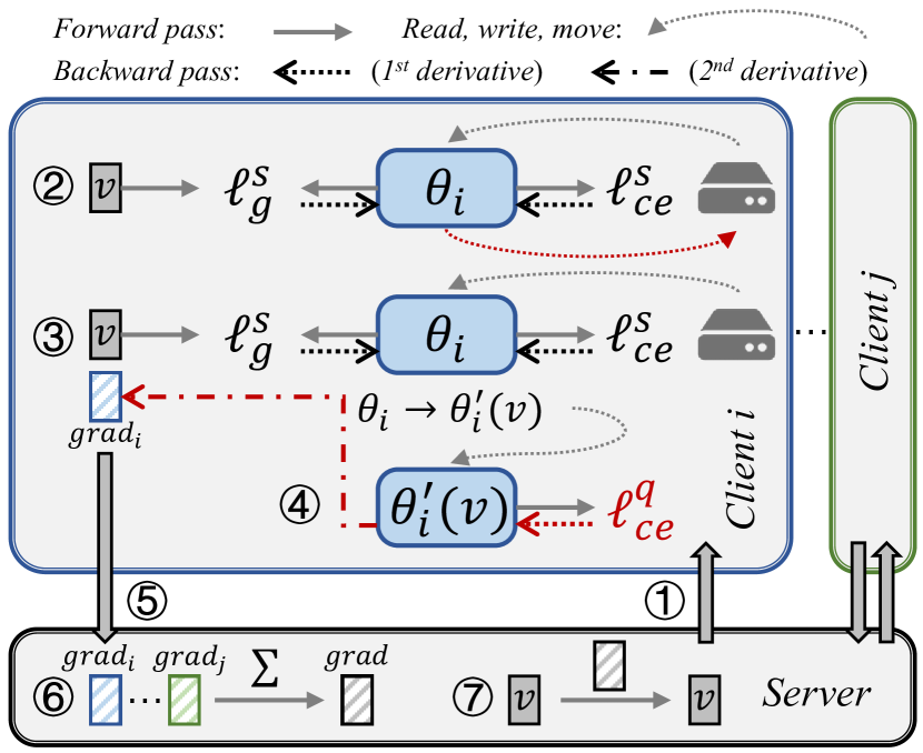
Figure 2: Seven steps of FedL2G in one iteration. $\ell^{s}$ and $\ell^{q}$ denote the loss computed on the study and quiz sets, respectively. For clarity, we only show one $v$ of $\mathcal{G}$ and omit the $y$ and $t$ superscripts of $v$ here. The color red indicates emphasis. Best viewed in color.

Warm-up period.   Since $\mathcal{G}$ is randomly initialized, using an uninformative $\mathcal{G}$ misguides local model training in Eq. 4. Therefore, before conducting regular client training in step , FedL2G requires a warm-up period of $T^{\prime}$ iterations ($T^{\prime}=50$ is enough) with step , , , , , . Without step , the warm-up process only involves one batch of each client’s quiz set, thus demanding relatively small computation overhead.

Twin HtFL methods based on FedL2G.   The above processes assume sharing information in the logit space, denoted as FedL2G-l. Additionally, when considering the intermediate feature space, we can rephrase all the corresponding $\ell_{g}$, for instance, rewriting $\ell_{g}(h_{i}({\bm{x}},{\bm{\theta}}^{h}_{i}),{\bm{v}}^{y})$ in Eq. 4, where $h_{i}$ represents the feature extractor component in $f_{i}$, ${\bm{\theta}}^{h}_{i}\subset{\bm{\theta}}_{i}$ denotes the associated model parameters, and ${\bm{v}}^{y}$ resides in the intermediate feature space. We denote this twin method as FedL2G-f. The server learning rate $\eta_{s}$ is the unique hyperparameter in our FedL2G-l or FedL2G-f. Due to space constraints, we offer a detailed algorithm of our FedL2G-l in Algorithm 1. Extending it to FedL2G-f only requires necessary substitutions.

Algorithm 1 The Learning Processes in FedL2G-l

1:$N$ clients; initial parameters ${\bm{\theta}}^{0}_{1},\ldots,{\bm{\theta}}^{0}_{N}$ and $\mathcal{G}^{0}=\{{\bm{v}}^{y,0}\}_{y=1}^{C}$; $\eta_{c}$: local learning rate; $\eta_{s}$: server learning rate; $\rho$: client joining ratio; $E$: local epochs; $T$: total communication iterations.

2:Well-trained client model parameters ${\bm{\theta}}_{1},\ldots,{\bm{\theta}}_{N}$.

3:All clients split their training data into a study set $\mathcal{D}^{s}$ and a batch of quiz set $\mathcal{D}^{q}$.

4:for communication iteration $t=1,\ldots,T$ do

5:     Server samples a client subset $\mathcal{I}^{t}$ based on $\rho$.

6:     Server sends $\mathcal{G}^{t-1}$ to each client in $\mathcal{I}^{t}$.

7:     for Client $i\in\mathcal{I}^{t}$ in parallel do

8:         if $t>T^{\prime}$ then

9:              Updates ${\bm{\theta}}^{t-1}_{i}$ to ${\bm{\theta}}^{t}_{i}$ using SGD for $E$ epochs via

10:      $\min_{{\bm{\theta}}_{i}}\ \mathbb{E}_{({\bm{x}},y)\sim\mathcal{D}^{s}_{i}}[\ell_{ce}(f_{i}({\bm{x}},{\bm{\theta}}^{t-1}_{i}),y)+\ell_{g}(f_{i}({\bm{x}},{\bm{\theta}}^{t-1}_{i}),{\bm{v}}^{y,t-1})]$

11:         else

12:              Marks ${\bm{\theta}}^{t-1}_{i}$ as ${\bm{\theta}}^{t}_{i}$.          

13:         Executes a pseudo-train step on a randomly sampled batch $\mathcal{B}^{s}_{i}$ via Eq. 5 with ${\bm{\theta}}^{t}_{i}$.

14:         Computes the gradients of $\mathcal{G}^{t-1}$, i.e., $\pi^{t}_{i}$, on $\mathcal{D}^{q}_{i}$ via Eq. 7.

15:         Sends non-zero vectors among $\pi^{t}_{i}$ to the server.      

16:     Server averages the non-zero vectors of $\pi^{t}_{i},i\in\mathcal{I}^{t}$ for each class to obtain $\pi^{t}$.

17:     Server updates $\mathcal{G}^{t-1}$ to $\mathcal{G}^{t}$ via $\mathcal{G}^{t}=\mathcal{G}^{t-1}-\eta_{s}\pi^{t}$.

18:return ${\bm{\theta}}^{T}_{1},\ldots,{\bm{\theta}}^{T}_{N}$.

3.3 Efficiency Analysis

As we compute gradients for two different entities in the outer-loop and inner-loop, respectively, we eliminate the necessity for calculating the second-order gradients of model parameters w.r.t. $\ell_{ce}$ as well as the associated computationally intensive Hessian (Fallah et al., 2020b). Our analysis is founded on Assumption 1 and Assumption 2 in Appendix C. Due to space limit, we leave the derivative details to Eq. C.11 and show client $i$’s gradient w.r.t. $\mathcal{G}$ here:

$$\pi_{i}=-\eta_{c}\mathbb{E}_{({\bm{x}},y)\sim\mathcal{D}^{q}_{i}}\{\nabla_{1}\ell_{ce}\cdot\nabla_{2}f_{i}\cdot\mathbb{E}_{({\bm{x}}^{\prime},y^{\prime})\sim\mathcal{B}^{s}_{i}}[\nabla_{2}f_{i}\cdot{\color[rgb]{1,0,0}\nabla_{\mathcal{G}^{t-1}}\nabla_{1}\ell_{g}}]\},$$ (7)

where $\nabla_{1}\ell_{ce}:=\nabla_{a_{1}}\ell_{ce}(a_{1},a_{2})$, indicating the derivative of $\ell_{ce}$ w.r.t. the first variable, and so for $\nabla_{2}f_{i}$ and $\nabla_{1}\ell_{g}$. The operation $\cdot$ denotes multiplication. Computing $\nabla_{1}\ell_{ce}$ and $\nabla_{2}f_{i}$ is a common practice in deep learning (Zhang & Sabuncu, 2018) and calculating the ${\color[rgb]{1,0,0}\nabla_{\mathcal{G}^{t-1}}\nabla_{1}\ell_{g}}$ term is pivotal. To simplify the calculation, we choose the MSE loss as our $\ell_{g}$, so $\ell_{g}(f_{i}({\bm{x}}^{\prime},{\bm{\theta}}_{i}),{\bm{v}}^{y^{\prime}})=\frac{1}{M}\sum_{m=1}^{M}[f_{i}({\bm{x}}^{\prime},{\bm{\theta}}_{i})_{m}-{\bm{v}}^{y^{\prime}}_{m}]^{2}$, where $M$ is the dimension of ${\bm{v}}^{y^{\prime}}$. Given $\mathcal{G}=\{{\bm{v}}^{y}\}_{y=1}^{C}$, we have

$${\color[rgb]{1,0,0}\nabla_{\mathcal{G}^{t-1}}\nabla_{1}\ell_{g}}=\frac{2}{M}\sum_{m=1}^{M}\nabla_{\mathcal{G}^{t-1}}(f_{i}({\bm{x}}^{\prime},{\bm{\theta}}_{i})_{m}-{\bm{v}}^{y^{\prime}}_{m})=\frac{2}{M}\sum_{m=1}^{M}-1={\color[rgb]{1,0,0}-2}.$$ (8)

Finally, we obtain

$$\pi_{i}=2\eta_{c}\mathbb{E}_{({\bm{x}},y)\sim\mathcal{D}^{q}_{i}}\{\nabla_{1}\ell_{ce}\cdot\nabla_{2}f_{i}\cdot\mathbb{E}_{({\bm{x}}^{\prime},y^{\prime})\sim\mathcal{B}^{s}_{i}}[\nabla_{2}f_{i}]\},$$ (9)

where only first-order derivatives of $f_{i}$ w.r.t. ${\bm{\theta}}_{i}$ are required.

3.4 Convergence Analysis

Given notations, assumptions, and proofs in Appendix C, we have

Theorem 1 (One-iteration deviation).

Let Assumption 1 to Assumption 3 hold. For an arbitrary client, after every communication iteration, we have

$$\mathbb{E}[\mathcal{L}^{(t+1)E+1/2}]\leq\mathcal{L}^{tE+1/2}+(\frac{L_{1}\eta_{c}^{2}}{2}-\eta_{c})\sum_{e=1/2}^{E-1}||\nabla\mathcal{L}^{tE+e}||_{2}^{2}+\frac{L_{1}E\eta_{c}^{2}\sigma^{2}}{2}+2\eta_{c}^{2}\eta_{s}L_{2}R^{\prime}ER.$$

Theorem 2 (Non-convex convergence rate of FedL2G).

Let Assumption 1 to Assumption 3 hold and $\Delta=\mathcal{L}^{0}-\mathcal{L}^{*}$, where $\mathcal{L}^{*}$ refers to the local optimum. Given Theorem 1, for an arbitrary client and an arbitrary constant $\epsilon$, our FedL2G has a non-convex convergence rate $\mathcal{O}(1/T)$ with

$$\frac{1}{T}\sum_{t=0}^{T-1}\sum_{e=1/2}^{E-1}\mathbb{E}[||\nabla\mathcal{L}^{tE+e}||_{2}^{2}]\leq\frac{\frac{2\Delta}{T}+L_{1}E\eta_{c}^{2}\sigma^{2}+4\eta_{c}^{2}\eta_{s}L_{2}R^{\prime}ER}{2\eta_{c}-L_{1}\eta_{c}^{2}}<\epsilon,$$

where $0<\eta_{c}<\frac{2\epsilon}{L_{1}(E\sigma^{2}+\epsilon)+4\eta_{s}L_{2}R^{\prime}ER}$ and $\eta_{s}>0$.

According to Theorem 2, our FedL2G can converge at a rate of $\mathcal{O}(1/T)$, and the server learning rate $\eta_{s}$ can be set to any positive value.

4 Experiments

To evaluate the performance of our FedL2G-l and FedL2G-f alongside six popular server-lightweight HtFL methods: LG-FedAvg (Liang et al., 2020), FedGH (Yi et al., 2023), FML (Shen et al., 2020), FedKD (Wu et al., 2022), FedDistill (Jeong et al., 2018), and FedProto (Tan et al., 2022b), we conduct comprehensive experiments on four public datasets under two widely used data heterogeneity settings, involving up to 14 heterogeneous model architectures. Specifically, we demonstrate the encouraging performance of FedL2G in accuracy, communication cost, and computation cost. Subsequently, we investigate the characteristics behind our FedL2G from an experimental perspective.

Data heterogeneity settings.   Following existing work (Zhang et al., 2023d; Lin et al., 2020; Zhang et al., 2023b; 2024a), we adopt two popular settings across four enduring datasets Cifar10 (Krizhevsky & Geoffrey, 2009), Cifar100 (Krizhevsky & Geoffrey, 2009), Flowers102 (Nilsback & Zisserman, 2008), and Tiny-ImageNet (Chrabaszcz et al., 2017). Concretely, we simulate pathological data heterogeneity settings by allocating sub-datasets with 2/10/10/20 classes of data from Cifar10/Cifar100/Flowers102/Tiny-ImageNet to each client. In Dirichlet data heterogeneity settings, we allocate the data of class $y$ to each client using a client-specific ratio $q^{y}$ from a given dataset. $q^{y}$ is sampled from a Dirichlet distribution with a control parameter $\beta$ as described in (Lin et al., 2020). By default, we set $\beta=0.1$ for Cifar10 and Cifar100, and $\beta=0.01$ for Flowers102 and Tiny-ImageNet to enhance setting diversity. In both the pathological and Dirichlet settings, the data quantity among clients varies to account for unbalanced scenarios.

Model heterogeneity settings.   To neatly denote model heterogeneity settings, we utilize the notation HtFE_X following the convention in (Zhang et al., 2024b) to represent a group of heterogeneous feature extractors, where $X$ denotes the degree of model heterogeneity (positive correlation), while the remaining classifier heads remain homogeneous. For example, HtFE₈ denotes a group of eight heterogeneous feature extractors from eight model architectures (4-layer CNN (McMahan et al., 2017), GoogleNet (Szegedy et al., 2015), MobileNet_v2 (Sandler et al., 2018), ResNet18, ResNet34, ResNet50, ResNet101, and ResNet152 (He et al., 2016)), respectively. In addition, we use the notation HtM_X to denote a group of fully heterogeneous models. Within a specific group, for instance, HtFE_X, we allocate the $(i\mod X)$th model in this group to client $i$ with reinitialized parameters. Given the popularity of all models within HtFE₈ in the FL field, our primary focus is on utilizing HtFE₈. Additionally, some baseline methods, such as LG-FedAvg and FedGH, assume the classifier heads to be homogeneous, making HtM_X inapplicable for them. Moreover, to meet the prerequisite of identical feature dimensions ($K$) for FedGH, FedKD, and FedProto, we incorporate an average pooling layer (Szegedy et al., 2015) before the classifier heads and set $K=512$ for all models.

Other necessary settings.   Following common practice (McMahan et al., 2017), we execute a complete local training epoch with a batch size of 10, i.e., $\lfloor\frac{n_{i}}{10}\rfloor$ update steps, during each communication iteration. We conduct each experiment for up to 1000 iterations across three trials, employing a client learning rate ($\eta_{c}$) of 0.01, and present the best results with error bars. Moreover, we examine full participation ($\rho=1$), for 20 clients, while setting partial participation ($\rho=0.5$) for scenarios involving 50 and 100 clients. Please refer to the Appendix A for more details and results.

4.1 Accuracy in Two Data Heterogeneity Settings

Table 1: The test accuracy (%) on four datasets in two data heterogeneity settings using HtFE₈.

Settings	Pathological Setting				Dirichlet Setting
Datasets	C10	C100	F102	TINY	C10	C100	F102	TINY
LG-FedAvg	86.8$\pm$.3	57.0$\pm$.7	58.9$\pm$.3	32.0$\pm$.2	84.6$\pm$.5	40.7$\pm$.1	70.0$\pm$.9	48.2$\pm$.1
FedGH	86.6$\pm$.2	57.2$\pm$.2	59.3$\pm$.3	32.6$\pm$.4	84.4$\pm$.3	41.0$\pm$.5	69.7$\pm$.2	46.7$\pm$.1
FML	87.1$\pm$.2	55.2$\pm$.1	57.8$\pm$.3	31.4$\pm$.2	85.9$\pm$.1	39.9$\pm$.3	68.4$\pm$1.2	47.1$\pm$.1
FedKD	87.3$\pm$.3	56.6$\pm$.3	54.8$\pm$.4	32.6$\pm$.4	86.5$\pm$.2	40.6$\pm$.3	69.6$\pm$1.6	48.2$\pm$.5
FedDistill	87.2$\pm$.1	57.0$\pm$.3	58.5$\pm$.3	31.5$\pm$.4	86.0$\pm$.3	41.5$\pm$.1	71.2$\pm$.7	48.8$\pm$.1
FedProto	83.4$\pm$.2	53.6$\pm$.3	55.1$\pm$.2	29.3$\pm$.4	82.1$\pm$1.7	36.3$\pm$.3	62.3$\pm$.6	40.0$\pm$.1
FedL2G-l	87.7$\pm$.1	59.2$\pm$.4	60.3$\pm$.9	32.8$\pm$.7	86.5$\pm$.1	42.3$\pm$.1	71.5$\pm$.5	49.5$\pm$.3
FedL2G-f	89.3$\pm$.2	64.2$\pm$.3	64.2$\pm$.2	34.7$\pm$.3	87.6$\pm$.2	43.8$\pm$.4	73.6$\pm$.3	50.3$\pm$.4

To save space, we utilize brief abbreviations to represent the dataset names, specifically: “C10” for Cifar10, “C100” for Cifar100, “F102” for Flowers102, and “TINY” for Tiny-ImageNet. Based on Tab. 1, both FedL2G-l and FedL2G-f show superior performance compared to baseline methods. Notably, FedL2G-f demonstrates better performance across all datasets and scenarios. This can be attributed to the fact that FedL2G-l learns to guide the original local task in the logit space, while FedL2G-f focuses on the intermediate feature space, and the latter contains richer information due to its higher dimension. In terms of accuracy, FedL2G-f surpasses the best baseline FedGH on Cifar100 by 7.0% (a percentage improvement of 12.2%) in the pathological setting. Methods based on mutual distillation, such as FML and FedKD, transfer more information (with more bits) than other methods in each iteration, yet they do not consistently achieve optimal performance due to the absence of a teacher model with prior knowledge. FedProto suffers in the model heterogeneity setting and performs the worst, as client models exhibit varying feature extraction abilities (Zhang et al., 2024a). Conversely, our FedL2G-f excels with learning-to-guide in the intermediate feature space. While FedDistill mitigates this issue by sharing prototypical logits, there is still room for improvement through learning-to-guide in the logit space, a capability offered by FedL2G-l.

4.2 Accuracy in Additional Five Model Heterogeneity Settings

Table 2: The test accuracy (%) on Cifar100 in the default Dirichlet setting with incremental degrees of model heterogeneity or more clients.

Settings	Incremental Degrees of Model Heterogeneity					More Clients ($\rho=0.5$)
	HtFE2	HtFE3	HtFE4	HtFE9	HtM10	$N=50$	$N=100$
LG-FedAvg	46.6$\pm$.2	45.6$\pm$.4	43.9$\pm$.2	42.0$\pm$.3	—	37.8$\pm$.1	35.1$\pm$.5
FedGH	46.7$\pm$.4	45.2$\pm$.2	43.3$\pm$.2	43.0$\pm$.9	—	37.3$\pm$.4	34.3$\pm$.2
FML	45.9$\pm$.2	43.1$\pm$.1	43.0$\pm$.1	42.4$\pm$.3	39.9$\pm$.1	38.8$\pm$.1	36.1$\pm$.3
FedKD	46.3$\pm$.2	43.2$\pm$.5	43.2$\pm$.4	42.3$\pm$.4	40.4$\pm$.1	38.3$\pm$.4	35.6$\pm$.6
FedDistill	46.9$\pm$.1	43.5$\pm$.2	43.6$\pm$.1	42.1$\pm$.2	41.0$\pm$.1	38.5$\pm$.4	36.1$\pm$.2
FedProto	44.0$\pm$.2	38.1$\pm$.6	34.7$\pm$.6	32.7$\pm$.8	36.1$\pm$.1	33.0$\pm$.4	29.0$\pm$.5
FedL2G-l	47.3$\pm$.1	44.5$\pm$.1	44.8$\pm$.1	44.1$\pm$.1	41.8$\pm$.2	38.9$\pm$.2	36.7$\pm$.1
FedL2G-f	47.8$\pm$.3	45.8$\pm$.1	44.7$\pm$.1	45.7$\pm$.2	43.5$\pm$.1	40.5$\pm$.0	37.9$\pm$.3

Besides the HtFE₈ group, we also explore five other model heterogeneity settings, while maintaining consistent data heterogeneity in the Dirichlet setting to control variables. The degree of model heterogeneity escalates from HtFE₂ to HtM₁₀ as follows: HtFE₂ comprises 4-layer CNN and ResNet18; HtFE₃ includes ResNet10 (Zhong et al., 2017), ResNet18, and ResNet34; HtFE₄ comprises 4-layer CNN, GoogleNet, MobileNet_v2, and ResNet18; HtFE₉ includes ResNet4, ResNet6, and ResNet8 (Zhong et al., 2017), ResNet10, ResNet18, ResNet34, ResNet50, ResNet101, and ResNet152; HtM₁₀ contains all the model architectures in HtFE₈ plus two additional architectures ViT-B/16 (Dosovitskiy et al., 2020) and ViT-B/32 (Dosovitskiy et al., 2020). ViT models have a complex classifier head, whereas other CNN-based models only consider the last fully connected layer as the classifier head. Consequently, methods assuming a homogeneous classifier head, such as LG-FedAvg and FedGH, do not apply to HtM₁₀. Referring to Tab. 2, our FedL2G-l and FedL2G-f continue to perform well in these scenarios, particularly in more model-heterogeneous settings. As the setting becomes more heterogeneous, it becomes increasingly challenging to find consistent knowledge to share, and negative transfer (Cui et al., 2022) may also arise. However, the knowledge of learning-to-guide is generic, making it easy for FedL2G to aggregate and distribute this knowledge in diverse scenarios, benefiting all clients.

4.3 Accuracy With More Clients or More Local Training Epochs

More Clients.   In addition to experimenting with a total of 20 clients, we extend our evaluation by incorporating more clients created using the given Cifar100 dataset. With an increase in the number of clients, maintaining a consistent total data amount across all clients results in less local data on each client. In these scenarios, with a partial client participation ratio of $\rho=0.5$, our FedL2G-l and FedL2G-f can still maintain their superiority, as shown in Tab. 2.

More Local Training Epochs.   Increasing the number of local epochs, denoted by $E$, in each communication iteration can reduce the total number of iterations required for convergence, consequently lowering total communication overhead (McMahan et al., 2017; Zhang et al., 2024b). In Tab. 3, FedGH experiences approximately a 1% decrease in accuracy when $E\geq 10$. Since the globally shared model struggles with data heterogeneity, FML and FedKD also exhibit performance degradation with a larger $E$, albeit to a more severe extent. Specifically, both FML and FedKD continue to decrease from $E=5$ to $E=20$, with FML dropping by 3.1% and FedKD dropping by 2.0%. In contrast, our FedL2G-l and FedL2G-f consistently uphold their superior performance even with a larger $E$. Remarkably, FedL2G-f shows an increase of 0.6% in accuracy from $E=5$ to $E=20$, showcasing its exceptional adaptability in scenarios with low communication quality.

Table 3: The test accuracy (%) on Cifar100 in the default Dirichlet setting using HtFE₈ for three experiments. “MB” and “s” are short for megabyte and second, respectively. The time in the brackets represents the warm-up period cost, which is several times less than local training.

Experiments	Local Training Epochs			Comm. (MB)		Computation (s)
	$E=5$	$E=10$	$E=20$	Up.	Down.	Client	Server
LG-FedAvg	40.3$\pm$.2	40.5$\pm$.1	40.9$\pm$.2	3.93	3.93	6.18	0.04
FedGH	41.1$\pm$.3	39.9$\pm$.3	40.2$\pm$.4	1.75	3.93	9.53	0.37
FML	39.1$\pm$.3	38.0$\pm$.2	36.0$\pm$.2	70.57	70.57	8.63	0.07
FedKD	41.1$\pm$.1	40.4$\pm$.2	39.1$\pm$.3	63.02	63.02	9.04	0.07
FedDistill	41.0$\pm$.3	41.3$\pm$.2	41.1$\pm$.4	0.34	0.76	6.52	0.03
FedProto	38.0$\pm$.5	38.1$\pm$.4	38.7$\pm$.5	1.75	3.89	6.65	0.04
FedL2G-l	42.2$\pm$.2	42.0$\pm$.2	42.1$\pm$.1	0.34	0.76	7.49 (2.23)	0.03
FedL2G-f	43.7$\pm$.1	43.8$\pm$.2	44.3$\pm$.3	1.75	3.89	8.84 (2.24)	0.04

4.4 Communication and Computation Overhead

Communication cost.   We consider both the upload and download bytes (across all participating clients) as part of the communication overhead in each iteration, using a float32 (= 4 bytes) data type in PyTorch (Paszke et al., 2019) to store each floating number. In Tab. 3, despite FML and FedKD transmitting a relatively small global model, their communication costs remain significantly high compared to other methods that share lightweight components. The SVD technique in FedKD (Wu et al., 2022), does not significantly reduce the communication overhead. Given that we only upload the gradients of guiding vectors on the client, the communication cost of FedL2G-l and FedL2G-f is equivalent to that of FedDistill and FedProto, respectively. This cost falls within the lowest group among these methods.

Computation cost.   To capture essential operations, we measure the averaged GPU execution time of each client and the server on an idle GPU card in each iteration and show the time cost in Tab. 3. As FedGH gathers prototypes after local training, it costs extra time for inferencing across the entire training set using the trained client model. In contrast, FedDistill and FedProto collect prototypical logits and features, respectively, concurrently with model training in each batch, thereby eliminating this additional cost. Besides, FedGH trains the global head on the server consuming relatively more power, even with one server epoch per iteration. Since we only average gradients on the server and update $\mathcal{G}$ once without backpropagation, our FedL2G-l and FedL2G-f demonstrate similar time-efficiency to FedDistill and FedProto, respectively. Due to the extra learning-to-guide process, FedL2G costs more client time than FedDistill and FedProto. However, FedL2G-l still requires less time than FML, FedKD, and FedGH, and the improved test accuracy justifies this cost.

4.5 FedL2G Prioritizes the Original Task

Beyond presenting the test accuracy, we delve into the intrinsic training process by examining the training losses. For each method, we illustrate only the original local loss, i.e., $\ell_{ce}$, in Fig. 3. Specifically, we aggregate the original local losses of all the clients through weighted averaging, following Eq. 1. These original local loss curves closely align with the accuracy trends in Tab. 2 (HtFE₉), indicating that lower original local loss corresponds to higher test accuracy in our scenarios. Since our FedL2G learns guiding vectors that help the client model focus more on its original task, FedL2G-l and FedL2G-f achieve the second-lowest and lowest losses, respectively.

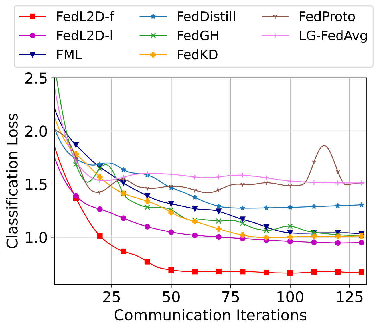
Figure 3: The averaged original local loss ($\ell_{ce}$) of all clients for nine HtFL methods on Cifar100 in the default Dirichlet setting using HtFE₉.

Besides the magnitude of the original local losses, our FedL2G method also offers advantages in smoothness and convergence speed. From Fig. 3, we observe that the loss curves of FedDistill, FedGH, FedProto, and LG-FedAvg fluctuate significantly in the beginning. The growth of $\ell_{ce}$ can be attributed to the mismatch of the shared global information and clients’ tasks. Given that FedL2G-l and FedL2G-f focus on clients’ original tasks, we can introduce more client-required information for guiding vectors, leading to a stable reduction in the original local loss. Because of the same benefits, FedL2G-f can converge at a relatively early iteration and simultaneously achieve the highest test accuracy. Despite the lesser amount of guiding information in FedL2G-l compared to FedL2G-f, FedL2G-l also demonstrates superiority in terms of smoothness and convergence when compared to FedDistill.

4.6 FedL2G Protects Feature Information

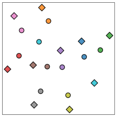
(a) FedL2G-l.

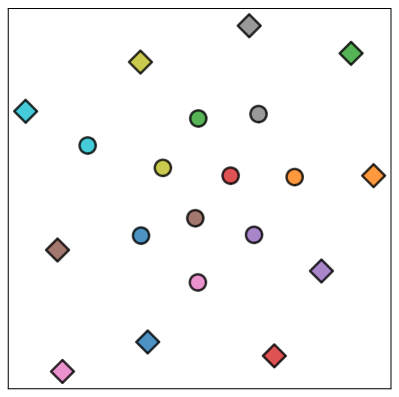
(b) FedL2G-f.

Figure 4: The t-SNE visualization of guiding vectors (diamonds) and feature vectors (circles) on Cifar10 in the default Dirichlet setting using HtFE₈. Different colors represent different classes. Best viewed in color.

Differing from FedDistill and FedProto, which gather data-derived prototypical logits and features from the clients, we collect the gradients of randomly initialized guiding vectors. These gradients are calculated using a complex formula (refer to Eq. 7) to reduce the original local losses for all clients. Therefore, our FedL2G does not directly upload data-related information from clients and safeguards the feature information for clients. In a sense, logit vectors are also feature vectors with lower dimensions. Here, we illustrate the t-SNE (Van der Maaten & Hinton, 2008) visualization of the global prototypes $\{{\bm{g}}^{y}\}_{y=1}^{C}$ (obtained via Eq. 2) and the guiding vectors $\{{\bm{v}}^{y}\}_{y=1}^{C}$ from FedL2G-l and FedL2G-f. As per Fig. 4, guiding vectors differ from global prototypes in that they do not overlap. Moreover, guiding vectors and global prototypes of the same class do not always cluster together. Instead, guiding vectors and global prototypes from different classes can be closer, providing additional protection for the class information of local features. This phenomenon is more pronounced in FedL2G-f, where the distances between guiding vectors and global prototypes are larger than that in FedL2G-l. This is because the guiding vectors in FedL2G-f have relatively more parameters and knowledge to learn. Given that a larger distance signifies improved discrimination and guidance for the class-wise vectors utilized in a guiding loss (Zhang et al., 2024a), our guiding vectors exhibit greater separability than the global prototypes, indicating enhanced guidance capability for the client models.

5 Conclusion

We observe the original local loss growth phenomenon on the client in prior prototype-based HtFL methods when guided by global prototypes. Then we attribute this problem to the mismatch between the guiding objective and the client’s original local objective. To address this issue, we propose a FedL2G approach to reduce the client’s original objective when using guiding vectors by giving priority to the local objective during the learning of guiding vectors. The superiority of FedL2G is evidenced through theoretical analysis and extensive experiments.

Appendix A Additional Experimental Details

Datasets and environment.   We use four datasets with their respective download links: Cifar10, Cifar100, Flowers102, and Tiny-ImageNet. We split all client data into a training set and a test set with a ratio of 75% and 25%, respectively, on each client, and we evaluate the averaged test accuracy on clients’ test sets. All our experiments are conducted on a machine with 64 Intel(R) Xeon(R) Platinum 8362 CPUs, 256G memory, eight NVIDIA 3090 GPUs, and Ubuntu 20.04.4 LTS. Most of our experiments can be completed within 48 hours, while others, involving a large number of clients and extensive local training epochs, may take up to a week to finish.

Hyperparameter settings.   For our baseline methods, we set their hyperparameters following existing work (Zhang et al., 2024a; b). As for our FedL2G-l and FedL2G-f, we tune the server learning rate $\eta_{s}$ (the unique hyperparameter) by grid search on the Cifar100 dataset in the default Dirichlet setting with HtFE₈ and use an identical setting on all experimental tasks without further tuning. Specifically, we search $\eta_{s}$ in the range: $\{0.01,0.05,0.1,0.5,1,10,50,100,500\}$. We set $\eta_{s}=0.1$ for FedL2G-l and set $\eta_{s}=100$ for FedL2G-f. The $\eta_{s}$ hyperparameters of FedL2G-l and FedL2G-f differ due to their discrepancy in the learnable knowledge capacity of the guiding vectors. The dimension of the guiding vectors in FedL2G-f is larger than in FedL2G-l, necessitating more server updates.

The small auxiliary model for FML and FedKD.   As FML and FedKD utilize a global auxiliary model for mutual distillation, this auxiliary model needs to be as compact as possible to minimize communication overhead during model parameter transmission (Wu et al., 2022). Therefore, we opt for the smallest model within each group of heterogeneous models to serve as the auxiliary model in all scenarios.

Appendix B Sensitivity Study

To further study the influence of the server learning rate $\eta_{s}$, we conduct a sensitivity study here. From Tab. 4, we know that FedL2G-l and FedL2G-f benefit from distinct ranges of $\eta_{s}$, which is also attributed to their different trainable parameters and learning capacities. Moreover, FedL2G-f demonstrates higher optimal accuracy than FedL2G-l, while FedL2G-l yields a more stable outcome across different $\eta_{s}$.

	$\eta_{s}=0.01$	$\eta_{s}=0.05$	$\eta_{s}=0.1$	$\eta_{s}=0.5$	$\eta_{s}=1$
FedL2G-l	41.7$\pm$.3	41.6$\pm$.1	42.3$\pm$.1	41.6$\pm$.5	41.8$\pm$.3
	$\eta_{s}=1$	$\eta_{s}=10$	$\eta_{s}=50$	$\eta_{s}=100$	$\eta_{s}=500$
FedL2G-f	41.1$\pm$.5	42.0$\pm$.1	43.5$\pm$.1	43.8$\pm$.4	41.4$\pm$.5

Table 4: The test accuracy (%) of FedL2G-l and FedL2G-f on Cifar100 in the default Dirichlet setting using HtFE₈ with different $\eta_{s}$.

Appendix C Theoretical Analysis

Here we bring some existing equations for convenience. Recall that we have $N$ clients training their heterogeneous local models (with parameters ${\bm{\theta}}_{1},\ldots,{\bm{\theta}}_{N}$) using their private and heterogeneous training data $\mathcal{D}_{1},\ldots,\mathcal{D}_{N}$. Besides, they share global guiding vectors $\mathcal{G}=\{{\bm{v}}^{y}\}_{y=1}^{C}$, with the assistance of a server to facilitate collaborative learning. Formally, the objective of FedL2G is

$$\min_{{\bm{\theta}}_{1},\ldots,{\bm{\theta}}_{N}}\ \sum_{i=1}^{N}\frac{|\mathcal{D}_{i}|}{n}\mathcal{L}_{\mathcal{D}_{i}}({\bm{\theta}}_{i},\mathcal{G}),$$ (C.1)

where the total client loss $\mathcal{L}_{\mathcal{D}_{i}}$ is defined by

$$\mathcal{L}_{\mathcal{D}_{i}}({\bm{\theta}}_{i},\mathcal{G}):=\mathbb{E}_{({\bm{x}},y)\sim\mathcal{D}_{i}}[\ell_{ce}(f_{i}({\bm{x}},{\bm{\theta}}_{i}),y)+\ell_{g}(f_{i}({\bm{x}},{\bm{\theta}}_{i}),{\bm{v}}^{y})],$$ (C.2)

and the original local loss $\mathcal{L}^{\prime}_{\mathcal{D}_{i}}$ is defined by

$$\mathcal{L}^{\prime}_{\mathcal{D}_{i}}({\bm{\theta}}_{i},\mathcal{G}):=\mathbb{E}_{({\bm{x}},y)\sim\mathcal{D}_{i}}[\ell_{ce}(f_{i}({\bm{x}},{\bm{\theta}}_{i}),y)].$$ (C.3)

Here we consider FedL2G-l for simplicity, and it is easy to extend theoretical analysis to FedL2G-f by substituting $\ell_{g}(f_{i}({\bm{x}},{\bm{\theta}}_{i}),{\bm{v}}^{y})$ with $\ell_{g}(h_{i}({\bm{x}},{\bm{\theta}}_{i}^{h}),{\bm{v}}^{y})$. We optimize global $\mathcal{G}$ by

$$\mathcal{G}^{t}=\mathcal{G}^{t-1}-\eta_{s}\frac{1}{N}\sum_{i\in[N]}\nabla_{\mathcal{G}^{t-1}}\mathbb{E}_{({\bm{x}},y)\sim\mathcal{D}^{q}_{i}}[\ell_{ce}(f_{i}({\bm{x}},{\bm{\theta}}_{i}-\eta_{c}\nabla_{{\bm{\theta}}_{i}}\mathcal{L}_{\mathcal{B}^{s}_{i}}({\bm{\theta}}_{i},\mathcal{G}^{t-1})),y)],$$ (C.4)

where we consider full participation for simplicity. The convergence of Eq. C.2 for any client is equivalent to the convergence of FedL2G’s objective in Eq. C.1. Thus, we omit the client notation $i$ and some corresponding notations, such as $\mathcal{D}_{i}$, in the following.

To further examine the local training process, in addition to the communication iteration notation $t$, we introduce $e\in\{1/2,1,2,\ldots,E\}$ to represent the local step. We denote the $e$th local training step in iteration $t$ as $tE+e$. Specifically, $tE+1/2$ refers to the moment when clients receive $\mathcal{G}$ before local training. We adopt four assumptions, partially based on FedProto (Tan et al., 2022b).

Assumption 1 (Unbiased Gradient and Bounded Variance).

The stochastic gradient $\omega^{t}=\nabla\mathcal{L}_{\xi}({\bm{\theta}}^{t},\mathcal{G}^{t})$ is an unbiased estimation of each client’s gradient w.r.t. its loss:

$$\mathbb{E}_{\xi\sim\mathcal{D}}[\omega^{t}]=\nabla\mathcal{L}({\bm{\theta}}^{t},\mathcal{G})=\nabla\mathcal{L}^{t}.$$

and its variance is bounded by $\sigma^{2}$:

$$\mathbb{E}[||\omega^{t}-\nabla\mathcal{L}^{t}||_{2}^{2}]\leq\sigma^{2}.$$

Assumption 2 (Bounded Gradient).

The expectation of the stochastic gradient $\omega^{t}$ and $\omega^{\prime t}=\nabla\mathcal{L}^{\prime}_{\xi}({\bm{\theta}}^{t},\mathcal{G}^{t})$ are bounded by $R$ and $R^{\prime}$, respectively:

$$\mathbb{E}[||\omega^{t}||_{2}]\leq R,\quad\mathbb{E}[||\omega^{\prime t}||_{2}]\leq R^{\prime}.$$

Assumption 3 (Lipschitz Smoothness).

Each total local objective $\mathcal{L}$ is $L_{1}$-Lipschitz smooth, which also means the gradient of $\mathcal{L}$ is $L_{1}$-Lipschitz continuous, i.e.,

$$||\nabla\mathcal{L}^{t_{1}}-\nabla\mathcal{L}^{t_{2}}||_{2}\leq L_{1}||{\bm{\theta}}^{t_{1}}-{\bm{\theta}}^{t_{2}}||_{2},\quad\forall t_{1},t_{2}>0,$$

which implies the following quadratic bound,

$$\mathcal{L}^{t_{1}}-\mathcal{L}^{t_{2}}\leq\left<\nabla\mathcal{L}^{t_{2}},({\bm{\theta}}^{t_{1}}-{\bm{\theta}}^{t_{2}})\right>+\frac{1}{2}L_{1}||{\bm{\theta}}^{t_{1}}-{\bm{\theta}}^{t_{2}}||_{2}^{2},\quad\forall t_{1},t_{2}>0.$$

Besides, each client model function $f$ is $L_{2}$-Lipschitz smooth, i.e.,

$$||\nabla f^{t_{1}}-\nabla f^{t_{2}}||_{2}\leq L_{2}||{\bm{\theta}}^{t_{1}}-{\bm{\theta}}^{t_{2}}||_{2},\quad\forall t_{1},t_{2}>0.$$

Given Assumption 1 and Assumption 2, any client’s gradient w.r.t. $\mathcal{G}$ is

$$\pi^{t-1} =\nabla_{\mathcal{G}^{t-1}}\mathbb{E}_{({\bm{x}},y)\sim\mathcal{D}^{q}}[\ell_{ce}(f({\bm{x}},{\bm{\theta}}-\eta_{c}\nabla_{{\bm{\theta}}}\mathcal{L}_{\mathcal{B}^{s}}({\bm{\theta}},\mathcal{G}^{t-1})),y)]$$ (C.5)

$$=\mathbb{E}_{({\bm{x}},y)\sim\mathcal{D}^{q}}[\nabla_{\mathcal{G}^{t-1}}\ell_{ce}(f({\bm{x}},{\bm{\theta}}-\eta_{c}\nabla_{{\bm{\theta}}}\mathcal{L}_{\mathcal{B}^{s}}({\bm{\theta}},\mathcal{G}^{t-1})),y)]$$ (C.6)

$$=\mathbb{E}_{({\bm{x}},y)\sim\mathcal{D}^{q}}[\nabla_{1}\ell_{ce}\cdot\nabla_{2}f\cdot\nabla_{\mathcal{G}^{t-1}}({\bm{\theta}}-\eta_{c}\nabla_{{\bm{\theta}}}\mathcal{L}_{\mathcal{B}^{s}}({\bm{\theta}},\mathcal{G}^{t-1}))]$$ (C.7)

$$=-\eta_{c}\mathbb{E}_{({\bm{x}},y)\sim\mathcal{D}^{q}}[\nabla_{1}\ell_{ce}\cdot\nabla_{2}f\cdot\nabla_{\mathcal{G}^{t-1}}\nabla_{{\bm{\theta}}}\mathcal{L}_{\mathcal{B}^{s}}({\bm{\theta}},\mathcal{G}^{t-1})]$$ (C.8)

$$=-\eta_{c}\mathbb{E}_{({\bm{x}},y)\sim\mathcal{D}^{q}}\{\nabla_{1}\ell_{ce}\cdot\nabla_{2}f\cdot\mathbb{E}_{({\bm{x}}^{\prime},y^{\prime})\sim\mathcal{B}^{s}}[\nabla_{\mathcal{G}^{t-1}}\nabla_{{\bm{\theta}}}\ell_{g}(f({\bm{x}}^{\prime},{\bm{\theta}}),{\bm{v}}^{y^{\prime}})]\}$$ (C.9)

$$=-\eta_{c}\mathbb{E}_{({\bm{x}},y)\sim\mathcal{D}^{q}}\{\nabla_{1}\ell_{ce}\cdot\nabla_{2}f\cdot\mathbb{E}_{({\bm{x}}^{\prime},y^{\prime})\sim\mathcal{B}^{s}}[\nabla_{2}f\cdot\nabla_{\mathcal{G}^{t-1}}\nabla_{1}\ell_{g}]\}$$ (C.10)

$$=2\eta_{c}\mathbb{E}_{({\bm{x}},y)\sim\mathcal{D}^{q}}\{\nabla_{1}\ell_{ce}\cdot\nabla_{2}f\cdot\mathbb{E}_{({\bm{x}}^{\prime},y^{\prime})\sim\mathcal{B}^{s}}[\nabla_{2}f]\},$$ (C.11)

where $\nabla_{1}\ell_{ce}:=\nabla_{a_{1}}\ell_{ce}(a_{1},a_{2})$, indicating the derivative of $\ell_{ce}$ w.r.t. the first variable, and so for $\nabla_{2}f$ and $\nabla_{1}\ell_{g}$. Under Assumption 1, we can mimic regular training through the pseudo-train step , as $\mathcal{B}^{s}$ is randomly re-sampled in each iteration. All the derivatives in Eq. C.11 are bounded under Assumption 2.

Then, we have two key lemmas:

Lemma 1.

Let Assumption 1 and Assumption 3 hold. The total client loss of an arbitrary client can be bounded:

$$\mathbb{E}[\mathcal{L}^{(t+1)E}]\leq\mathcal{L}^{tE+1/2}+(\frac{L_{1}\eta_{c}^{2}}{2}-\eta_{c})\sum_{e=1/2}^{E-1}||\nabla\mathcal{L}^{tE+e}||_{2}^{2}+\frac{L_{1}E\eta_{c}^{2}\sigma^{2}}{2}.$$

Proof.

This lemma focuses solely on local training at the client level, incorporating both the original local objective and the guiding objective. It can be easily derived by substituting the relevant notations from Lemma 1 of the prototype-based HtFL method, FedProto. ∎

Lemma 2.

Let Assumption 2 and Assumption 3 hold. After the guiding vectors are updated on the server and downloaded to clients, the total client loss of an arbitrary client can be bounded:

$$\mathbb{E}[\mathcal{L}^{(t+1)E+1/2}]\leq\mathcal{L}^{(t+1)E}+2\eta_{c}^{2}\eta_{s}L_{2}R^{\prime}ER.$$

Proof.

$$\mathcal{L}^{(t+1)E+1/2} =\mathcal{L}^{(t+1)E}+\mathcal{L}^{(t+1)E+1/2}-\mathcal{L}^{(t+1)E}$$ (C.12)

$$=\mathcal{L}^{(t+1)E}+||f({\bm{\theta}}^{(t+1)E})-\mathcal{G}^{(t+2)E}||_{2}-||f({\bm{\theta}}^{(t+1)E})-\mathcal{G}^{(t+1)E}||_{2}$$ (C.13)

$$\stackrel{{\scriptstyle(a)}}{{\leq}}\mathcal{L}^{(t+1)E}+||\mathcal{G}^{(t+2)E}-\mathcal{G}^{(t+1)E}||_{2}$$ (C.14)

$$=\mathcal{L}^{(t+1)E}+\eta_{s}||\mathbb{E}_{[N]}(\pi^{(t+1)E}-\pi^{(t+2)E})||_{2}$$ (C.15)

$$\stackrel{{\scriptstyle(b)}}{{\leq}}\mathcal{L}^{(t+1)E}+\eta_{s}\mathbb{E}_{[N]}||\pi^{(t+1)E}-\pi^{(t+2)E}||_{2}$$ (C.16)

$$\stackrel{{\scriptstyle(c)}}{{\leq}}\mathcal{L}^{(t+1)E}+2\eta_{c}\eta_{s}\mathbb{E}_{[N]}\mathbb{E}_{\mathcal{D}}||\nabla_{1}\ell_{ce}^{(t+1)E}\cdot\nabla_{2}f^{(t+1)E}\cdot\mathbb{E}_{\xi}[\nabla_{2}f^{(t+1)E}]-\nabla_{1}\ell_{ce}^{tE}\cdot\nabla_{2}f^{tE}\cdot\mathbb{E}_{\xi}[\nabla_{2}f^{tE}]||_{2}$$ (C.17)

$$\stackrel{{\scriptstyle(d)}}{{\leq}}\mathcal{L}^{(t+1)E}+2\eta_{c}\eta_{s}R^{\prime}\mathbb{E}_{[N]}\mathbb{E}_{\xi}||\nabla_{2}f^{(t+1)E}-\nabla_{2}f^{tE}||_{2}$$ (C.18)

$$\stackrel{{\scriptstyle(e)}}{{\leq}}\mathcal{L}^{(t+1)E}+2\eta_{c}\eta_{s}L_{2}R^{\prime}\mathbb{E}_{[N]}\mathbb{E}_{\xi}||{\bm{\theta}}^{(t+1)E}-{\bm{\theta}}^{tE}||_{2}$$ (C.19)

$$\stackrel{{\scriptstyle(f)}}{{\leq}}\mathcal{L}^{(t+1)E}+2\eta_{c}^{2}\eta_{s}L_{2}R^{\prime}\mathbb{E}_{[N]}\mathbb{E}_{\xi}\sum_{e=1/2}^{E-1}||\omega^{tE+e}||_{2}$$ (C.20)

Take expectations of random variable $\xi$, we have

$$\mathbb{E}[\mathcal{L}^{(t+1)E+1/2}] \leq\mathcal{L}^{(t+1)E}+2\eta_{c}^{2}\eta_{s}L_{2}R^{\prime}\mathbb{E}_{[N]}\mathbb{E}_{\xi}\sum_{e=1/2}^{E-1}||\omega^{tE+e}||_{2}$$ (C.21)

$$\stackrel{{\scriptstyle(g)}}{{\leq}}\mathcal{L}^{(t+1)E}+2\eta_{c}^{2}\eta_{s}L_{2}R^{\prime}ER.$$ (C.22)

In the above inequations, (a) follows from $||a-b||_{2}-||a-c||_{2}\leq||b-c||_{2}$; (b), (c), and (f) follow from $||\sum a_{j}||_{2}\leq\sum||a_{j}||_{2}$, where $\mathbb{E}_{\mathcal{D}}a$ denotes taking expectations of $a$ over set $\mathcal{D}$, e.g., $\mathbb{E}_{[N]}a$ means $\mathbb{E}_{i\sim\{1,\ldots,N\}}a_{j}$; (d) follows from Assumption 1 and Assumption 2, where $\mathcal{L}^{\prime}({\bm{\theta}},\mathcal{G})=\nabla_{1}\ell_{ce}\cdot\nabla_{2}f$; (e) follows from Assumption 3; (g) follows from Assumption 2. ∎

Then, we have

Theorem 1 (One-iteration deviation).

Let Assumption 1 to Assumption 3 hold. For an arbitrary client, after every communication iteration, we have

$$\mathbb{E}[\mathcal{L}^{(t+1)E+1/2}]\leq\mathcal{L}^{tE+1/2}+(\frac{L_{1}\eta_{c}^{2}}{2}-\eta_{c})\sum_{e=1/2}^{E-1}||\nabla\mathcal{L}^{tE+e}||_{2}^{2}+\frac{L_{1}E\eta_{c}^{2}\sigma^{2}}{2}+2\eta_{c}^{2}\eta_{s}L_{2}R^{\prime}ER.$$

Proof.

Taking expectation of ${\bm{\theta}}$ on both sides in Lemma 2, we have

$$\mathbb{E}[\mathcal{L}^{(t+1)E+1/2}]\leq\mathbb{E}[\mathcal{L}^{(t+1)E}]+2\eta_{c}^{2}\eta_{s}L_{2}R^{\prime}ER.$$ (C.23)

Then summing Eq. C.23 and Lemma 1 up, we have

$$\mathbb{E}[\mathcal{L}^{(t+1)E+1/2}]\leq\mathcal{L}^{tE+1/2}+(\frac{L_{1}\eta_{c}^{2}}{2}-\eta_{c})\sum_{e=1/2}^{E-1}||\nabla\mathcal{L}^{tE+e}||_{2}^{2}+\frac{L_{1}E\eta_{c}^{2}\sigma^{2}}{2}+2\eta_{c}^{2}\eta_{s}L_{2}R^{\prime}ER.$$ (C.24)

∎

Theorem 2 (Non-convex convergence rate of FedL2G).

Let Assumption 1 to Assumption 3 hold and $\Delta=\mathcal{L}^{0}-\mathcal{L}^{*}$, where $\mathcal{L}^{*}$ refers to the local optimum. Given Theorem 1, for an arbitrary client and an arbitrary constant $\epsilon$, our FedL2G has a non-convex convergence rate $\mathcal{O}(1/T)$ with

$$\frac{1}{T}\sum_{t=0}^{T-1}\sum_{e=1/2}^{E-1}\mathbb{E}[||\nabla\mathcal{L}^{tE+e}||_{2}^{2}]\leq\frac{\frac{2\Delta}{T}+L_{1}E\eta_{c}^{2}\sigma^{2}+4\eta_{c}^{2}\eta_{s}L_{2}R^{\prime}ER}{2\eta_{c}-L_{1}\eta_{c}^{2}}<\epsilon,$$

where $0<\eta_{c}<\frac{2\epsilon}{L_{1}(E\sigma^{2}+\epsilon)+4\eta_{s}L_{2}R^{\prime}ER}$ and $\eta_{s}>0$.

Proof.

By interchanging the left and right sides of Eq. C.24, we can get

$$\sum_{e=1/2}^{E-1}||\nabla\mathcal{L}^{tE+e}||_{2}^{2}\leq\frac{\mathcal{L}^{tE+1/2}-\mathbb{E}[\mathcal{L}^{(t+1)E+1/2}]+\frac{L_{1}E\eta_{c}^{2}\sigma^{2}}{2}+2\eta_{c}^{2}\eta_{s}L_{2}R^{\prime}ER}{\eta_{c}-\frac{L_{1}\eta_{c}^{2}}{2}},$$ (C.25)

when $\eta_{c}-\frac{L_{1}\eta_{c}^{2}}{2}>0$, i.e., $0<\eta_{c}<\frac{2}{L_{1}}$. Taking the expectation of ${\bm{\theta}}$ on both sides and summing all inequalities overall communication iterations, we obtain

$$\frac{1}{T}\sum_{t=0}^{T-1}\sum_{e=1/2}^{E-1}\mathbb{E}[||\nabla\mathcal{L}^{tE+e}||_{2}^{2}]\leq\frac{\frac{1}{T}\sum_{t=0}^{T-1}(\mathcal{L}^{tE+1/2}-\mathbb{E}[\mathcal{L}^{(t+1)E+1/2}])+\frac{L_{1}E\eta_{c}^{2}\sigma^{2}}{2}+2\eta_{c}^{2}\eta_{s}L_{2}R^{\prime}ER}{\eta_{c}-\frac{L_{1}\eta_{c}^{2}}{2}}.$$ (C.26)

Let $\Delta=\mathcal{L}^{0}-\mathcal{L}^{*}>0$, we have $\frac{1}{T}\sum_{t=0}^{T-1}(\mathcal{L}^{tE+1/2}-\mathbb{E}[\mathcal{L}^{(t+1)E+1/2}])\leq\Delta$ and

$$\frac{1}{T}\sum_{t=0}^{T-1}\sum_{e=1/2}^{E-1}\mathbb{E}[||\nabla\mathcal{L}^{tE+e}||_{2}^{2}]\leq\frac{\frac{2\Delta}{T}+L_{1}E\eta_{c}^{2}\sigma^{2}+4\eta_{c}^{2}\eta_{s}L_{2}R^{\prime}ER}{2\eta_{c}-L_{1}\eta_{c}^{2}}.$$ (C.27)

Given any $\epsilon>0$, let

$$\frac{\frac{2\Delta}{T}+L_{1}E\eta_{c}^{2}\sigma^{2}+4\eta_{c}^{2}\eta_{s}L_{2}R^{\prime}ER}{2\eta_{c}-L_{1}\eta_{c}^{2}}<\epsilon,$$ (C.28)

we have

$$T>\frac{2\Delta}{\epsilon\eta_{c}(2-L_{1}\eta_{c})-\eta_{c}^{2}(L_{1}E\sigma^{2}+4\eta_{s}L_{2}R^{\prime}ER)}.$$ (C.29)

In this context, we have

$$\frac{1}{T}\sum_{t=0}^{T-1}\sum_{e=1/2}^{E-1}\mathbb{E}[||\nabla\mathcal{L}^{tE+e}||_{2}^{2}]\leq\epsilon,$$ (C.30)

when

$$0<\eta_{c}<\frac{2\epsilon}{L_{1}(E\sigma^{2}+\epsilon)+4\eta_{s}L_{2}R^{\prime}ER}<\frac{2}{L_{1}},$$ (C.31)

and

$$\eta_{s}>0$$ (C.32)

Since all the notations of the right side in Eq. C.27 are given constants except for $T$, our FedL2G’s non-convex convergence rate is $\epsilon\sim\mathcal{O}(1/T)$. ∎

Appendix D Visualizations of Data Distributions

We illustrate the data distributions on all clients in the experiments in the following.

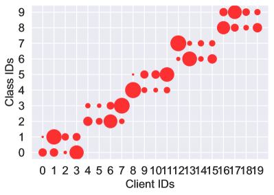
(a) Cifar10

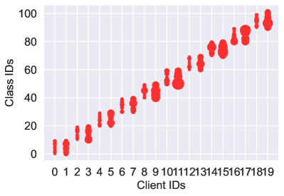
(b) Flowers102

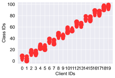
(c) Cifar100

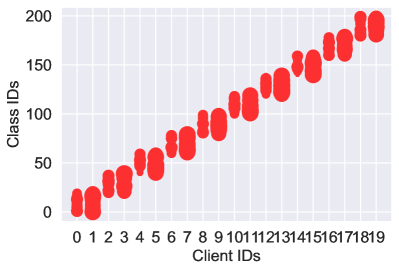
(d) Tiny-ImageNet

Figure 5: The data distribution of each client on Cifar10, Flowers102, Cifar100, and Tiny-ImageNet, respectively, in the pathological settings. The size of a circle represents the number of samples.

(a) Cifar10

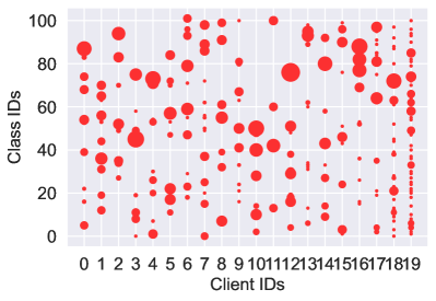
(b) Flowers102

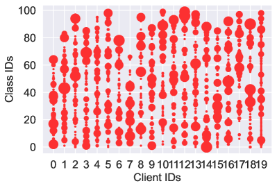
(c) Cifar100

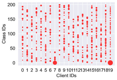
(d) Tiny-ImageNet

Figure 6: The data distribution of each client on Cifar10 ($\beta=0.1$), Flowers102 ($\beta=0.01$), Cifar100 ($\beta=0.1$), and Tiny-ImageNet ($\beta=0.01$), respectively, in Dirichlet setting s. The size of a circle represents the number of samples.

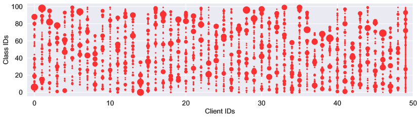
(a) 50 clients

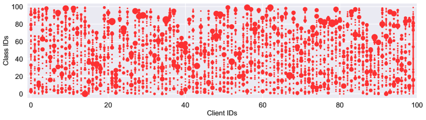
(b) 100 clients

Figure 7: The data distribution of each client on Cifar100 in the Dirichlet setting ($\beta=0.1$) with 50 and 100 clients, respectively. The size of a circle represents the number of samples.

References

- Achiam et al. (2023) Josh Achiam, Steven Adler, Sandhini Agarwal, Lama Ahmad, Ilge Akkaya, Florencia Leoni Aleman, Diogo Almeida, Janko Altenschmidt, Sam Altman, Shyamal Anadkat, et al. Gpt-4 technical report. arXiv preprint arXiv:2303.08774, 2023.
- Chrabaszcz et al. (2017) Patryk Chrabaszcz, Ilya Loshchilov, and Frank Hutter. A Downsampled Variant of Imagenet as an Alternative to the Cifar Datasets. arXiv preprint arXiv:1707.08819, 2017.
- Cui et al. (2022) Sen Cui, Jian Liang, Weishen Pan, Kun Chen, Changshui Zhang, and Fei Wang. Collaboration equilibrium in federated learning. In Proceedings of ACM SIGKDD International Conference on Knowledge Discovery and Data Mining, 2022.
- Diao et al. (2020) Enmao Diao, Jie Ding, and Vahid Tarokh. Heterofl: Computation and communication efficient federated learning for heterogeneous clients. In International Conference on Learning Representations (ICLR), 2020.
- Dosovitskiy et al. (2020) Alexey Dosovitskiy, Lucas Beyer, Alexander Kolesnikov, Dirk Weissenborn, Xiaohua Zhai, Thomas Unterthiner, Mostafa Dehghani, Matthias Minderer, Georg Heigold, Sylvain Gelly, et al. An image is worth 16x16 words: Transformers for image recognition at scale. In International Conference on Learning Representations (ICLR), 2020.
- Fallah et al. (2020a) Alireza Fallah, Aryan Mokhtari, and Asuman Ozdaglar. Personalized Federated Learning with Theoretical Guarantees: A Model-Agnostic Meta-Learning Approach. In Advances in Neural Information Processing Systems (NeurIPS), 2020a.
- Fallah et al. (2020b) Alireza Fallah, Aryan Mokhtari, and Asuman Ozdaglar. On the convergence theory of gradient-based model-agnostic meta-learning algorithms. In International Conference on Artificial Intelligence and Statistics, 2020b.
- Finn et al. (2017) Chelsea Finn, Pieter Abbeel, and Sergey Levine. Model-Agnostic Meta-Learning for Fast Adaptation of Deep Networks. In International Conference on Machine Learning (ICML), 2017.
- Grefenstette et al. (2019) Edward Grefenstette, Brandon Amos, Denis Yarats, Phu Mon Htut, Artem Molchanov, Franziska Meier, Douwe Kiela, Kyunghyun Cho, and Soumith Chintala. Generalized inner loop meta-learning. arXiv preprint arXiv:1910.01727, 2019.
- He et al. (2016) Kaiming He, Xiangyu Zhang, Shaoqing Ren, and Jian Sun. Deep Residual Learning for Image Recognition. In IEEE Conference on Computer Vision and Pattern Recognition (CVPR), 2016.
- Horvath et al. (2021) Samuel Horvath, Stefanos Laskaridis, Mario Almeida, Ilias Leontiadis, Stylianos Venieris, and Nicholas Lane. Fjord: Fair and accurate federated learning under heterogeneous targets with ordered dropout. Advances in Neural Information Processing Systems (NeurIPS), 2021.
- Hu et al. (2022) Chengming Hu, Xuan Li, Dan Liu, Xi Chen, Ju Wang, and Xue Liu. Teacher-student architecture for knowledge learning: A survey. arXiv preprint arXiv:2210.17332, 2022.
- Jeong et al. (2018) Eunjeong Jeong, Seungeun Oh, Hyesung Kim, Jihong Park, Mehdi Bennis, and Seong-Lyun Kim. Communication-efficient on-device machine learning: Federated distillation and augmentation under non-iid private data. arXiv preprint arXiv:1811.11479, 2018.
- Jiang et al. (2019) Yihan Jiang, Jakub Konečnỳ, Keith Rush, and Sreeram Kannan. Improving federated learning personalization via model agnostic meta learning. arXiv preprint arXiv:1909.12488, 2019.
- Kairouz et al. (2019) Peter Kairouz, H Brendan McMahan, Brendan Avent, Aurélien Bellet, Mehdi Bennis, Arjun Nitin Bhagoji, Kallista Bonawitz, Zachary Charles, Graham Cormode, Rachel Cummings, et al. Advances and Open Problems in Federated Learning. arXiv preprint arXiv:1912.04977, 2019.
- Karimireddy et al. (2020) Sai Praneeth Karimireddy, Satyen Kale, Mehryar Mohri, Sashank Reddi, Sebastian Stich, and Ananda Theertha Suresh. Scaffold: Stochastic Controlled Averaging for Federated Learning. In International Conference on Machine Learning (ICML), 2020.
- Krizhevsky & Geoffrey (2009) Alex Krizhevsky and Hinton Geoffrey. Learning Multiple Layers of Features From Tiny Images. Technical Report, 2009.
- Lee et al. (2022) Hung-Yi Lee, Shang-Wen Li, and Thang Vu. Meta learning for natural language processing: A survey. In Proceedings of the 2022 Conference of the North American Chapter of the Association for Computational Linguistics: Human Language Technologies, 2022.
- Li et al. (2022) Qinbin Li, Yiqun Diao, Quan Chen, and Bingsheng He. Federated learning on non-iid data silos: An experimental study. In 2022 IEEE 38th international conference on data engineering (ICDE). IEEE, 2022.
- Li et al. (2020) Tian Li, Anit Kumar Sahu, Ameet Talwalkar, and Virginia Smith. Federated Learning: Challenges, Methods, and Future Directions. IEEE Signal Processing Magazine, 37(3):50–60, 2020.
- Li et al. (2021) Tian Li, Shengyuan Hu, Ahmad Beirami, and Virginia Smith. Ditto: Fair and Robust Federated Learning Through Personalization. In International Conference on Machine Learning (ICML), 2021.
- Liang et al. (2020) Paul Pu Liang, Terrance Liu, Liu Ziyin, Nicholas B Allen, Randy P Auerbach, David Brent, Ruslan Salakhutdinov, and Louis-Philippe Morency. Think locally, act globally: Federated learning with local and global representations. arXiv preprint arXiv:2001.01523, 2020.
- Lin et al. (2020) Tao Lin, Lingjing Kong, Sebastian U Stich, and Martin Jaggi. Ensemble distillation for robust model fusion in federated learning. Advances in Neural Information Processing Systems (NeurIPS), 33:2351–2363, 2020.
- Lu et al. (2023) Menglong Lu, Zhen Huang, Zhiliang Tian, Yunxiang Zhao, Xuanyu Fei, and Dongsheng Li. Meta-tsallis-entropy minimization: a new self-training approach for domain adaptation on text classification. In Proceedings of the Thirty-Second International Joint Conference on Artificial Intelligence, 2023.
- Luo et al. (2023) Kangyang Luo, Shuai Wang, Yexuan Fu, Xiang Li, Yunshi Lan, and Ming Gao. Dfrd: Data-free robustness distillation for heterogeneous federated learning. Advances in Neural Information Processing Systems (NeurIPS), 2023.
- Ma et al. (2022) Xinge Ma, Jin Wang, Liang-Chih Yu, and Xuejie Zhang. Knowledge distillation with reptile meta-learning for pretrained language model compression. In Proceedings of the 29th International Conference on Computational Linguistics, 2022.
- McMahan et al. (2017) Brendan McMahan, Eider Moore, Daniel Ramage, Seth Hampson, and Blaise Aguera y Arcas. Communication-Efficient Learning of Deep Networks from Decentralized Data. In International Conference on Artificial Intelligence and Statistics (AISTATS), 2017.
- Nguyen et al. (2021) Dinh C Nguyen, Ming Ding, Pubudu N Pathirana, Aruna Seneviratne, Jun Li, and H Vincent Poor. Federated Learning for Internet of Things: A Comprehensive Survey. IEEE Communications Surveys & Tutorials, 23(3):1622–1658, 2021.
- Nilsback & Zisserman (2008) Maria-Elena Nilsback and Andrew Zisserman. Automated flower classification over a large number of classes. In 2008 Sixth Indian conference on computer vision, graphics & image processing, pp. 722–729. IEEE, 2008.
- Paszke et al. (2019) Adam Paszke, Sam Gross, Francisco Massa, Adam Lerer, James Bradbury, Gregory Chanan, Trevor Killeen, Zeming Lin, Natalia Gimelshein, Luca Antiga, et al. Pytorch: An imperative style, high-performance deep learning library. Advances in Neural Information Processing Systems (NeurIPS), 2019.
- Sandler et al. (2018) Mark Sandler, Andrew Howard, Menglong Zhu, Andrey Zhmoginov, and Liang-Chieh Chen. Mobilenetv2: Inverted residuals and linear bottlenecks. In IEEE Conference on Computer Vision and Pattern Recognition (CVPR), 2018.
- Sengupta et al. (2023) Ayan Sengupta, Shantanu Dixit, Md Shad Akhtar, and Tanmoy Chakraborty. A good learner can teach better: Teacher-student collaborative knowledge distillation. In International Conference on Learning Representations (ICLR), 2023.
- Shen et al. (2020) Tao Shen, Jie Zhang, Xinkang Jia, Fengda Zhang, Gang Huang, Pan Zhou, Kun Kuang, Fei Wu, and Chao Wu. Federated mutual learning. arXiv preprint arXiv:2006.16765, 2020.
- Szegedy et al. (2015) Christian Szegedy, Wei Liu, Yangqing Jia, Pierre Sermanet, Scott Reed, Dragomir Anguelov, Dumitru Erhan, Vincent Vanhoucke, and Andrew Rabinovich. Going deeper with convolutions. In IEEE Conference on Computer Vision and Pattern Recognition (CVPR), 2015.
- Tan et al. (2022a) Alysa Ziying Tan, Han Yu, Lizhen Cui, and Qiang Yang. Towards Personalized Federated Learning. IEEE Transactions on Neural Networks and Learning Systems, 2022a. Early Access.
- Tan et al. (2022b) Yue Tan, Guodong Long, Lu Liu, Tianyi Zhou, Qinghua Lu, Jing Jiang, and Chengqi Zhang. Fedproto: Federated Prototype Learning across Heterogeneous Clients. In AAAI Conference on Artificial Intelligence (AAAI), 2022b.
- Touvron et al. (2023) Hugo Touvron, Thibaut Lavril, Gautier Izacard, Xavier Martinet, Marie-Anne Lachaux, Timothée Lacroix, Baptiste Rozière, Naman Goyal, Eric Hambro, Faisal Azhar, et al. Llama: Open and efficient foundation language models. arXiv preprint arXiv:2302.13971, 2023.
- Van der Maaten & Hinton (2008) Laurens Van der Maaten and Geoffrey Hinton. Visualizing Data Using T-SNE. Journal of Machine Learning Research, 9(11), 2008.
- Wen et al. (2022) Dingzhu Wen, Ki-Jun Jeon, and Kaibin Huang. Federated dropout—a simple approach for enabling federated learning on resource constrained devices. IEEE wireless communications letters, 11(5):923–927, 2022.
- Wu et al. (2022) Chuhan Wu, Fangzhao Wu, Lingjuan Lyu, Yongfeng Huang, and Xing Xie. Communication-efficient federated learning via knowledge distillation. Nature communications, 13(1):2032, 2022.
- Yang et al. (2024) Shunzhi Yang, Jinfeng Yang, MengChu Zhou, Zhenhua Huang, Wei-Shi Zheng, Xiong Yang, and Jin Ren. Learning from human educational wisdom: A student-centered knowledge distillation method. IEEE Transactions on Pattern Analysis and Machine Intelligence, 2024.
- Ye et al. (2023) Mang Ye, Xiuwen Fang, Bo Du, Pong C Yuen, and Dacheng Tao. Heterogeneous federated learning: State-of-the-art and research challenges. ACM Computing Surveys, 56(3):1–44, 2023.
- Ye et al. (2024) Rui Ye, Wenhao Wang, Jingyi Chai, Dihan Li, Zexi Li, Yinda Xu, Yaxin Du, Yanfeng Wang, and Siheng Chen. Openfedllm: Training large language models on decentralized private data via federated learning. arXiv preprint arXiv:2402.06954, 2024.
- Yi et al. (2023) Liping Yi, Gang Wang, Xiaoguang Liu, Zhuan Shi, and Han Yu. Fedgh: Heterogeneous federated learning with generalized global header. In Proceedings of the 31st ACM International Conference on Multimedia, 2023.
- Yi et al. (2024) Liping Yi, Han Yu, Chao Ren, Gang Wang, Xiaoguang Liu, and Xiaoxiao Li. Federated model heterogeneous matryoshka representation learning. arXiv preprint arXiv:2406.00488, 2024.
- Zhang et al. (2023a) Jianqing Zhang, Yang Hua, Jian Cao, Hao Wang, Tao Song, Zhengui Xue, Ruhui Ma, and Haibing Guan. Eliminating domain bias for federated learning in representation space. Advances in Neural Information Processing Systems (NeurIPS), 2023a.
- Zhang et al. (2023b) Jianqing Zhang, Yang Hua, Hao Wang, Tao Song, Zhengui Xue, Ruhui Ma, Jian Cao, and Haibing Guan. Gpfl: Simultaneously learning global and personalized feature information for personalized federated learning. In IEEE International Conference on Computer Vision (ICCV), 2023b.
- Zhang et al. (2023c) Jianqing Zhang, Yang Hua, Hao Wang, Tao Song, Zhengui Xue, Ruhui Ma, and Haibing Guan. Fedcp: Separating feature information for personalized federated learning via conditional policy. In Proceedings of ACM SIGKDD International Conference on Knowledge Discovery and Data Mining, 2023c.
- Zhang et al. (2023d) Jianqing Zhang, Yang Hua, Hao Wang, Tao Song, Zhengui Xue, Ruhui Ma, and Haibing Guan. FedALA: Adaptive Local Aggregation for Personalized Federated Learning. In AAAI Conference on Artificial Intelligence (AAAI), 2023d.
- Zhang et al. (2023e) Jianqing Zhang, Yang Liu, Yang Hua, Hao Wang, Tao Song, Zhengui Xue, Ruhui Ma, and Jian Cao. Pfllib: Personalized federated learning algorithm library. arXiv preprint arXiv:2312.04992, 2023e.
- Zhang et al. (2024a) Jianqing Zhang, Yang Liu, Yang Hua, and Jian Cao. Fedtgp: Trainable global prototypes with adaptive-margin-enhanced contrastive learning for data and model heterogeneity in federated learning. arXiv preprint arXiv:2401.03230, 2024a.
- Zhang et al. (2024b) Jianqing Zhang, Yang Liu, Yang Hua, and Jian Cao. An upload-efficient scheme for transferring knowledge from a server-side pre-trained generator to clients in heterogeneous federated learning. arXiv preprint arXiv:2403.15760, 2024b.
- Zhang et al. (2018) Ying Zhang, Tao Xiang, Timothy M Hospedales, and Huchuan Lu. Deep mutual learning. In IEEE Conference on Computer Vision and Pattern Recognition (CVPR), 2018.
- Zhang & Sabuncu (2018) Zhilu Zhang and Mert Sabuncu. Generalized Cross Entropy Loss for Training Deep Neural Networks With Noisy Labels. In Advances in Neural Information Processing Systems (NeurIPS), 2018.
- Zhong et al. (2017) Zilong Zhong, Jonathan Li, Lingfei Ma, Han Jiang, and He Zhao. Deep residual networks for hyperspectral image classification. In 2017 IEEE International Geoscience and Remote Sensing Symposium (IGARSS), pp. 1824–1827. IEEE, 2017.
- Zhou et al. (2023) Hanhan Zhou, Tian Lan, Guru Prasadh Venkataramani, and Wenbo Ding. Every parameter matters: Ensuring the convergence of federated learning with dynamic heterogeneous models reduction. Advances in Neural Information Processing Systems (NeurIPS), 2023.
- Zhou et al. (2022) Wangchunshu Zhou, Canwen Xu, and Julian McAuley. Bert learns to teach: Knowledge distillation with meta learning. In Proceedings of the 60th Annual Meeting of the Association for Computational Linguistics (Volume 1: Long Papers), 2022.
- Zhu et al. (2021) Zhuangdi Zhu, Junyuan Hong, and Jiayu Zhou. Data-Free Knowledge Distillation for Heterogeneous Federated Learning. In International Conference on Machine Learning (ICML), 2021.