On the Solution of Linearized Inverse Scattering Problems in Near-Field Microwave Imaging by Operator Inversion and Matched Filtering

Abstract

Microwave imaging is commonly based on the solution of linearized inverse scattering problems by matched-filtering algorithms, i.e., by applying the adjoint of the forward scattering operator to the observation data. A more rigorous approach is the explicit inversion of the forward scattering operator, which is performed in this work for quasi-monostatic imaging scenarios based on a planar plane-wave representation according to the Weyl-identity and hierarchical acceleration algorithms. The inversion is achieved by a regularized iterative linear system of equations solver, where irregular observations as well as full probe correction are supported. In the spatial image generation low-pass filtering can be considered in order to reduce imaging artifacts. A corresponding spectral back-projection algorithm and a spatial back-projection algorithm together with improved focusing operators are also introduced and the resulting image generation algorithms are analyzed and compared for a variety of examples, comprising both simulated and measured observation data.

I Introduction

The great benefits of microwave radiation up to the mm-wave bands are its non-ionizing character but still very good resolution capabilities as well as its potential of penetrating through clothing barriers and dielectric walls [Sheen.Sep.2001, Ahmed.Sep.2012]. Due to these properties, microwave-based imaging techniques are used in various areas such as medical imaging [Chandra.May2015, Tajik., Gilmore.Jun.2009], satellite remote sensing [LeVine.Dec.1999, Krieger.May2014], or non-destructive testing [Kharkovsky.Apr.2007, Lopez.Jun.2022, Brinkmann.Oct.2022]. In particular the concept of synthetic aperture radar (SAR) has been proven as a versatile and reliable method in this regard [Saurer.Oct.2022, Na.Oct.2023]. In SAR, the movement of a carrier platform, e.g., an airplane carrying the transmit and receive antennas is utilized in order to synthesize larger virtual apertures, which consequently lead to an increase of resolution in cross-range direction [Moreira.Mar.2013]. It is clear that this technique is conceptually interesting for various applications such as drone measurements [Punzet.May2022], automotive radar [Farhadi.Apr.2022], or freehand smartphone imaging [AlvarezNarciandi.Mar.2021]. However, for a successful adaption of SAR imaging to these applications, different challenges have to be overcome. This is mainly due to the fact that the data acquisition for these examples is subject to irregular sampling. The realization of flexible and computationally inexpensive reconstruction algorithms, which can handle the irregularities, is, thus, a task of increasing significance [Smith.Jan.2022].

Mathematically, radar and imaging algorithms rely commonly on the solution of a linearized inverse scattering problem, where, according to the Born approximation, independent scattering center distributions are assumed, which only interact with the incident field [Haynes.Jan.2024]. This linearization of the inverse source problem allows to express the scattered electric field as a convolution of the scattering center distribution of the target with the dyadic Green’s function of the underlying homogeneous space [Schnattinger.May2012]. Consequently, employing a plane-wave expansion leads to a diagonalization of the linearized integral operator and, hence, in theory a direct inversion of the inverse source problem is possible. However, even within the first-order Born approximation the forward operator exhibits a null-space [Devaney.2012] leading to uniqueness problems, and the efficient processing of irregularly distributed observation locations and arbitrary probe orientations still poses a great challenge.

The corresponding imaging algorithms can be divided into direct reconstruction methods by adjoint imaging, sometimes also referred to as matched filtering [Dyab.Oct.2013], and operator inversion algorithms. Regarding direct image reconstruction, the standard back-projection algorithm (BPA) [Ahmed.Apr.2014, Batra.Apr.2021], also known as delay and sum method [Pisa.Oct.2018, Alkhodary.May2016], is widely used mainly due to its robustness and ease of implementation. Computationally much more efficient than the BPA are Fourier transform based $\omega$-$k$-methods [Moreira.Mar.2013, Saurer.Jul.2022], which perform the back-projection on a plane-wave basis in the spatial frequency domain and which can consider spectral filtering functions in a straightforward way. For efficient evaluation together with regular observation grids, they rely typically on fast Fourier transforms (FFTs). An efficient treatment of irregular observation grids is, e.g., possible with non-uniform FFTs [Wang.Jan.2020] or utilizing the multi-level fast spectral domain algorithm (MLFSDA) in [Saurer.Jul.2022], which exhibits excellent computational efficiency due to the use of hierarchical multi-level schemes as employed in the multi-level fast multipole method (MLFMM) [Chew.2001].

Common operator inversion methods start with an initial guess of the scattering distribution directly in the spatial domain, which is then further improved in terms of noise suppression or contrast enhancement by iteratively minimizing a least mean squares cost functional [Kelly.Jul.2011, Zhao.Jul.1991, Roberts.Feb.2010]. Alternatively, one may work with a spectral propagating plane-wave decomposition of the forward operator, which allows to solve rather well-conditioned and very compact single-frequency inverse source problems [Schnattinger.Aug.2014, Neitz.May2019]. The solution process can here be effectively accelerated by hierarchical concepts as found in the MLFMM and the spatial images are created by coherent superposition of the single-frequency images, which may, e.g., be obtained by hierarchical disaggregation [Schnattinger.May2012]. While it is clear that operator inversion methods provide an estimate of the solution quality by evaluating the norm of the residual error vector, the iteration process itself is of course more time- and memory consuming than the adjoint imaging methods.

Dependent on the utilized field representation and the imaging configuration, it can occur that the adjoint operator is identical to the inverse operator. Formally, this can be achieved by diagonalization and normalization of the scattering operator, e.g., in the form of a plane-wave or spherical mode expansion of the observations. However, in practical configurations this is typically not feasible due to truncation effects, sampling implications, and probing antenna influences. Another way of improving the adjoint imaging methods is to work with modified imaging operators, which are, e.g., calibrated via the obtained point spread functions [Osipov.Sep.2013, Broquetas.May1998, Watanabe.Mar.2022].

The goal of this article is to study and demonstrate the imaging properties of operator inversion based algorithms and contrast them to the corresponding properties of adjoint imaging methods, where the focus is on practically relevant planar and quasi-planar imaging configurations. The utilized operator inversion method is working according to the concepts of the MLFSDA based $\omega$-$k$-algorithm [Saurer.Jul.2022] for the operator evaluations within the iterative solver and has, thus, the ability to handle irregular observation sample distributions and arbitrary probing antennas. For the adjoint imaging, the MLFSDA based $\omega$-$k$-algorithm is employed as it is, but a standard spatial BPA is used as well, where in particular different focusing operators are derived from the plane-wave based adjoint operator representation. The superiority of the operator inversion method over the direct reconstruction approaches is in particular demonstrated for irregular observation locations, where simulated and measured observation data is used. Moreover, it is shown that spectral low-pass filtering functions can effectively suppress imaging artifacts in all of the considered algorithms.

The rest of this article is organized as follows. The formulation and derivation of the various imaging algorithms are given in Section II. The obtained imaging results by utilizing simulated as well as measured observation data are presented and discussed in Section LABEL:sim_setup and Section LABEL:meas, respectively. Based on this, some conclusions are drawn in Section LABEL:concl.

II Formulation of the imaging algorithms

II-A Problem Statement and Planar Plane-Wave Representation

Consider a quasi-monostatic scattering scenario, where the transmitting antenna (Tx), generating the incident fields, and the receiving antenna (Rx), recording the scattered fields, are either collocated or very close to each other at observation positions $\boldsymbol{r}_{m}$ with $m=1,2,\dots,M$. As depicted in Fig. 1, it is assumed that the scattering centers and the Tx/Rx locations are well separated, thus, allowing to introduce a planar Huygens’ surface in between, which is well suited to define the local support of an equivalent plane-wave representation of the incident and scattered fields.

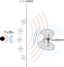
Figure 1: Visualization of the imaging scenario. The scattering behavior of an unknown object is equivalently described by utilizing a planar plane-wave expansion in the Huygens-plane $z=\mathrm{const}$.

Assuming the validity of the first-order Born approximation, the transfer operator between the two antennas via the scatterer can be written as [Schnattinger.Aug.2014]

$$T(\boldsymbol{r}_{m})=\iiint\limits_{V_{\mathrm{S}}}\boldsymbol{E}_{\mathrm{R}}\left({\boldsymbol{r}},\boldsymbol{r}_{m}\right)\cdot\boldsymbol{\bar{s}}_{\mathrm{B}}\left({\boldsymbol{r}}\right)\cdot\boldsymbol{E}_{\mathrm{T}}\left({\boldsymbol{r},\boldsymbol{r}_{m}}\right)\,\mathrm{d}^{3}\boldsymbol{r}\,,$$ (1)

where $\boldsymbol{\bar{s}}_{\mathrm{B}}\left({\boldsymbol{r}}\right)$ is the scattering dyad defined in the volume $V_{\mathrm{S}}$ at the position vector $\boldsymbol{r}=(x,y,z)$ with $r=\abs{\boldsymbol{r}}$, $\boldsymbol{E}_{\mathrm{T}}\left({\boldsymbol{r},\boldsymbol{r}_{m}}\right)$ is the radiated electric field vector of the Tx antenna, and $\boldsymbol{E}_{\mathrm{R}}\left({\boldsymbol{r}},\boldsymbol{r}_{m}\right)$ is the radiated electric field vector of the Rx antenna, which is reciprocal to the scattered field received by the Rx antenna. In order to arrive at a spectral representation of the scattering problem, we utilize the Weyl-identity in its original angular plane-wave spectrum form [Weyl1919, Booker1950]

$$\frac{\e^{-\mathrm{j}kr}}{r}=\frac{-\mathrm{j}k}{2\uppi}\iint\limits_{\Gamma}\e^{-\mathrm{j}k_{z}\abs{z}}\e^{-\mathrm{j}\left(k_{x}x+k_{y}y\right)}\,\mathrm{d}^{2}\hat{\boldsymbol{k}}\,$$ (2)

with an integration contour $\Gamma$ as explained and illustrated in Fig. 2, where the unit vector $\hat{\boldsymbol{{k}}}$ is oriented into the direction of the wave vector $\boldsymbol{k}=(k_{x},k_{y},k_{z})$ with $k=|\boldsymbol{k}|$. Assuming moreover a time dependence $\e^{\,\mathrm{j}\omega t}$ with angular frequency $\omega$, the radiated antenna fields incident on the scatterer can be expressed as [Saurer.Jul.2022, Kong1990, Eibert.2015]

$$\boldsymbol{E}_{\mathrm{T/R}}\left({\boldsymbol{r},\boldsymbol{r}_{m}}\right)=\iint\limits_{\Gamma^{\rm i}}\tilde{\boldsymbol{W}}_{\mathrm{T/R}}\left(\boldsymbol{k}^{\rm i}\right)\e^{-\mathrm{j}\boldsymbol{k}^{\rm i}\cdot\left(\boldsymbol{r}-\boldsymbol{r}_{m}\right)}\,\mathrm{d}^{2}\hat{\boldsymbol{k}}^{\rm i}\,$$ (3)

in terms of the angular plane-wave expansions $\tilde{\boldsymbol{W}}_{\mathrm{T}}\left(\boldsymbol{k}^{\rm i}\right)$ and $\tilde{\boldsymbol{W}}_{\mathrm{R}}\left(\boldsymbol{k}^{\rm i}\right)$ of the Tx and Rx antennas, respectively, which may be obtained from

$$\tilde{\boldsymbol{W}}_{\mathrm{T/R}}\left(\boldsymbol{k}^{\rm i}\right)=\frac{-Zk^{2}}{8\uppi^{2}}\left(\mathbf{\bar{I}}-\hat{\boldsymbol{k}}^{\rm i}\hat{\boldsymbol{k}}^{\rm i}\right)\cdot\iiint\limits_{V_{\mathrm{T/R}}}\boldsymbol{J}_{\mathrm{T/R}}\left(\boldsymbol{r}^{\prime}\right)\e^{\,\mathrm{j}\boldsymbol{k}^{\rm i}\cdot\boldsymbol{r}^{\prime}}\,\mathrm{d}^{3}\boldsymbol{r}^{\prime},$$ (4)

if $\boldsymbol{J}_{\mathrm{T/R}}(\boldsymbol{r}^{\prime})$ are corresponding spatial equivalent electric current densities producing the antenna radiation in free space. $Z=\sqrt{\mu/\varepsilon}$ is the wave impedance and $|\boldsymbol{k}^{\rm i}|=\omega\sqrt{\varepsilon\mu}$ the necessary dispersion relation, where $\varepsilon$ and $\mu$ are the permittivity and the permeability of the homogeneous background space, respectively. Assuming propagating plane waves towards the scatterer only, i.e., $\gamma$ on the integration contour shown in Fig. 2 ranging from 0 to $\uppi/2$, $\tilde{\boldsymbol{W}}_{\mathrm{T}}\left(\boldsymbol{k}^{\rm i}\right)$ and $\tilde{\boldsymbol{W}}_{\mathrm{R}}\left(\boldsymbol{k}^{\rm i}\right)$ correspond to the far-field patterns of the antennas.

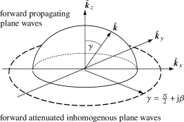
Figure 2: Integration contour $\Gamma$ in $k$-space for the angular spectrum evaluation of the Weyl-identity (2). The integration area is covered by integrating $\gamma$ from 0 to $\uppi/2$ and from $\uppi/2$ to $\uppi/2+\mathrm{j}\infty$ for a full $2\uppi$-integration of the rotation angle around the $\hat{\boldsymbol{k}}_{z}$-axis. The figure is slightly adapted from [Eibert.Jan.2024].

Typically both far-field patterns are expressed in spherical vector components according to

$$\tilde{\boldsymbol{W}}_{\mathrm{T/R}}\left(\boldsymbol{k}^{\rm i}\right)=\tilde{W}_{\mathrm{T/R}}^{\vartheta}\left(\boldsymbol{k}^{\rm i}\right)\hat{\boldsymbol{{\vartheta}}}+\tilde{W}_{\mathrm{T/R}}^{\varphi}\left(\boldsymbol{k}^{\rm i}\right)\hat{\boldsymbol{{\varphi}}}\,,$$ (5)

where $\hat{\boldsymbol{{\vartheta}}}$ and $\hat{\boldsymbol{{\varphi}}}$ are the corresponding spherical unit vectors. Plugging (3) into (1) and assuming the radiating reflectors model or correspondingly that the scattering process is purely monostatic in the $k$-space [Schnattinger.Aug.2014, Claerbout.1985], reduces the 4-D bistatic integral into a monostatic 2D integral and results in a spectral representation of the near-field transfer operator for polarimetric imaging in the form

$$T\left(\boldsymbol{r}_{m}\right)=\iint\limits_{\Gamma}\boldsymbol{\tilde{W}}_{\mathrm{R}}\left(-\boldsymbol{k}\right)\cdot\tilde{\boldsymbol{\bar{s}}}_{\mathrm{B}}\left(2\boldsymbol{k}\right)\cdot\boldsymbol{\tilde{W}}_{\mathrm{T}}\left(-\boldsymbol{k}\right)\e^{\,-\mathrm{j}2\boldsymbol{k}\cdot\boldsymbol{r}_{m}}\,\mathrm{d}^{2}\hat{\boldsymbol{k}}\,,$$ (6)

where $\boldsymbol{k}=-\boldsymbol{k}^{\rm i}$ has been introduced and where $\tilde{\boldsymbol{\bar{s}}}_{\mathrm{B}}\left(2\boldsymbol{k}\right)$ is the spectral scattering distribution defined as

$$\tilde{\boldsymbol{\bar{s}}}_{\mathrm{B}}\left(2\boldsymbol{k}\right)=\iiint\limits_{V_{\mathrm{S}}}\boldsymbol{\bar{s}}_{\mathrm{B}}\left(\boldsymbol{r}\right)\e^{\,\mathrm{j}2\boldsymbol{k}\cdot\boldsymbol{r}}\,\mathrm{d}^{3}\boldsymbol{r}\,.$$ (7)

Mapping of the integration contour $\Gamma$ of the Weyl-identity in (2) into the $(k_{x},k_{y})$-plane [Booker1950], results into its probably even more common planar plane-wave spectrum form [Kong1990]

$$\frac{\e^{-\mathrm{j}kr}}{r}=\iint\limits_{-\infty}^{+\infty}\frac{\e^{-\mathrm{j}k_{z}\abs{z}}}{2\uppi\mathrm{j}k_{z}}\e^{-\mathrm{j}\left(k_{x}x+k_{y}y\right)}\,\mathrm{d}{k}_{x}\mathrm{d}{k}_{y}\,.$$ (8)

Applying the same mapping to the near-field transfer or forward operator in (6) gives finally the planar plane-wave representation of the near-field transfer operator

$$T\left(\boldsymbol{r}_{m}\right)=\iint\limits_{-\infty}^{+\infty}\boldsymbol{\tilde{W}}_{\mathrm{R}}\left(-\boldsymbol{k}\right)\cdot\tilde{\boldsymbol{\bar{s}}}_{\mathrm{B}}\left(2\boldsymbol{k}\right)\cdot\boldsymbol{\tilde{W}}_{\mathrm{T}}\left(-\boldsymbol{k}\right)\frac{\e^{\,-\mathrm{j}2\boldsymbol{k}\cdot\boldsymbol{r}_{m}}}{kk_{z}}\,\mathrm{d}{k}_{x}\mathrm{d}{k}_{y},$$ (9)

which shall be the basis of our subsequent considerations. In literature, this equation is sometimes found with a $k_{z}^{2}$ in the denominator instead of the $k_{z}$. This may happen, if the derivation is carried out with the incident field (3) directly given in a planar plane-wave representation according to the Weyl-identity in (8), instead of (2). According to the concept of the angular spectrum of plane waves [Weyl1919, Booker1950], this is not correct. However, in terms of imaging, such a representation leads often even to better images, since the compensation of the $k_{z}^{2}$ in the denominator during the image generation is equivalent to a low-pass filtering of the image. In order to handle different Tx/Rx probing antenna combinations in a numerical implementation, the transfer or forward operator (9) is rewritten in a column vector format according to

$$T_{p}\left(\boldsymbol{r}_{m}\right)=\iint\limits_{-\infty}^{+\infty}\boldsymbol{\tilde{W}}_{p}\left(-\boldsymbol{k}\right)\cdot\tilde{\boldsymbol{S}}_{\mathrm{B}}\left(2\boldsymbol{k}\right)\frac{\e^{\,-\mathrm{j}2\boldsymbol{k}\cdot\boldsymbol{r}_{m}}}{kk_{z}}\,\mathrm{d}{k}_{x}\mathrm{d}{k}_{y}\,,$$ (10)

where the column vector $\boldsymbol{\tilde{W}}_{p}\left(-\boldsymbol{k}\right)$ contains the spectral probe weighting coefficients for the Tx/Rx probe combination $p$ with $p=1,2,\dots,P$ and the column vector $\tilde{\boldsymbol{S}}_{\mathrm{B}}(2\boldsymbol{k})$ contains the spherical scattering components of the dyad in (7). The 4-D column vector expressions are given as

$$\boldsymbol{\tilde{W}}_{p}\left(\boldsymbol{k}\right)=\left[\begin{array}[]{c}\tilde{W}_{\mathrm{R}_{p}}^{\vartheta}\left(\boldsymbol{k}\right)\tilde{W}_{\mathrm{T}_{p}}^{\vartheta}\left(\boldsymbol{k}\right)\vspace{0.1 cm}\\ \tilde{W}_{\mathrm{R}_{p}}^{\varphi}\left(\boldsymbol{k}\right)\tilde{W}_{\mathrm{T}_{p}}^{\varphi}\left(\boldsymbol{k}\right)\vspace{0.1cm}\\ \tilde{W}_{\mathrm{R}_{p}}^{\varphi}\left(\boldsymbol{k}\right)\tilde{W}_{\mathrm{T}_{p}}^{\vartheta}\left(\boldsymbol{k}\right)\vspace{0.1 cm}\\ \tilde{W}_{\mathrm{R}_{p}}^{\vartheta}\left(\boldsymbol{k}\right)\tilde{W}_{\mathrm{T}_{p}}^{\varphi}\left(\boldsymbol{k}\right)\end{array}\right],\,\,\tilde{\boldsymbol{S}}_{\mathrm{B}}\left(2\boldsymbol{k}\right)=\left[\begin{array}[]{c}\tilde{s}_{\vartheta\vartheta}\left(2\boldsymbol{k}\right)\\ \tilde{s}_{\varphi\varphi}\left(2\boldsymbol{k}\right)\\ \tilde{s}_{\varphi\vartheta}\left(2\boldsymbol{k}\right)\\ \tilde{s}_{\vartheta\varphi}\left(2\boldsymbol{k}\right)\end{array}\right]\,.$$

Utilizing the orthogonality of the plane waves in the observation plane $z=z_{m}$, the spectral scattering distribution is obtained from (10) according to

$$\boldsymbol{\tilde{W}}_{p}\left(-\boldsymbol{k}\right)\cdot\frac{\tilde{\boldsymbol{S}}_{\mathrm{B}}\left(2\boldsymbol{k}\right)}{kk_{z}}=\frac{1}{\uppi^{2}}\iint\limits_{-\infty}^{+\infty}T\left(\boldsymbol{r}_{m}\right)\\ \e^{\,\mathrm{j}2\boldsymbol{k}\cdot\boldsymbol{r}_{m}}\,\mathrm{d}x_{m}\mathrm{d}y_{m}$$ (11)

and the spatial scattering distribution is finally derived in the planar plane-wave representation S_B(r) & = 12 _-∞^+∞H_n(2k)~SB(2k)kkz^ -j2k⋅r dk_xdk_y
=14_-∞^+∞H_n(2k)[~W(-k)]^†⋅_-∞^+∞T(r_m)
                 ^ j2k⋅r_m dx_mdy_m   ^ -j2k⋅r dk_xdk_y , where $\boldsymbol{S}_{\mathrm{B}}(\boldsymbol{r})$ is the column vector representation of the scattering dyad $\boldsymbol{\bar{s}}_{\mathrm{B}}(\boldsymbol{r})$, $\boldsymbol{T}\left(\boldsymbol{r}_{m}\right)$ contains the scattering measurements obtained for different Tx/Rx probe antenna combinations in one vector, $H_{n}(2\boldsymbol{k})$ represents a low-pass filtering function, which can be used to mitigate artifacts due to the truncation of the plane-wave spectrum or the observation area [Devaney.2012]. $\boldsymbol{\tilde{W}}\left(-\boldsymbol{k}\right)$ denotes a probe correction matrix, which is obtained by stacking the vectors $\boldsymbol{\tilde{W}}_{p}\left(-\boldsymbol{k}\right)$ for $p=1,...,P$ row-wise in a matrix. Since this matrix can be severely ill-conditioned dependent on $\boldsymbol{k}$, its pseudo-inverse denoted by the symbol $\dagger$ is used in (11). This equation is the basis for the MLFSDA based $\omega$-$k$-algorithm as introduced in [Saurer.Jul.2022], where the final image is obtained by coherently summing up all the single-frequency images according to (11) for all considered frequencies. Due to its explicit inversion in the spectral domain, (11) can provide more accurate results than a standard adjoint operator evaluation. However, it is strictly correct only for measurements available in an infinite observation plane and for sets of Tx/Rx probe combinations with the same plane-wave spectrum in every measurement location $\boldsymbol{r}_{m}$. In practical implementations, the spatial integral over the observations in $\boldsymbol{T}(\boldsymbol{r}_{m})$ is often just performed as a discrete sum over the available observations where even 3-D irregular observation locations may be considered. Complications in the evaluation of (11) might arise from the computation of the pseudo-inverse of $\tilde{\boldsymbol{W}}(-\boldsymbol{k})$, which can be strongly rank deficient.

The low-pass filtering function $H_{n}(2\boldsymbol{k})={\left(2k_{z}\right)}^{n}$ with $n\in\mathbb{N}_{0}$ as introduced in (11) and (11) can help to improve the image quality. As will be shown later, the chosen form of filtering function allows for a closed-form representation of the focusing operator when utilizing the spatial back-projection algorithm. Since such a filtering operation reduces the bandwidth in the spatial frequency domain and, thus, also the achievable resolution in the reconstructed images, it should be used with care. In literature, such techniques are known as filtered back-projection methods [Devaney.2012].

II-B Iterative Operator Inversion

The operator inversion approach is starting from the near-field transfer operator as given in (10). In order to avoid numerical instabilities at the boundary of the visible region, it is convenient to define the auxiliary spectral scattering vector $\tilde{\boldsymbol{S}}_{\mathrm{B,inv}}(2\boldsymbol{k})$ = $\tilde{\boldsymbol{S}}_{\mathrm{B}}(2\boldsymbol{k})/k_{z}$, which is directly the quantity required to generate the image according to (11). The transverse spherical components of this vector are then discretized on a regular grid in $({k}_{x},k_{y})$ resulting into the $N$ spectral unknowns of the inverse problem, which are collected in the vector $\boldsymbol{x}\in\mathbb{C}^{N}$ and which are assumed to be defined with respect to an appropriately defined Huygens’ surface as, e.g., illustrated in Fig. 1. The $M$ observation samples according to $T_{p}(\boldsymbol{r}_{m})$ are stacked into the measurement vector $\boldsymbol{b}\in\mathbb{C}^{M}$. By defining the matrix $\boldsymbol{A}\in\mathbb{C}^{M\times N}$, which is the discrete numerical representation of the near-field transfer operator according to (10), a linear system of equations is obtained in the form $\boldsymbol{A}\boldsymbol{x}=\boldsymbol{b}$. Since this system of equations is typically at least mildly ill-posed and may have less or more unknowns than equations, it is solved in the form of the normal error system of equations

$$\boldsymbol{A}\boldsymbol{A}^{\mathrm{ad}}\,\boldsymbol{u}=\boldsymbol{b}\,,$$ (12)

where $\boldsymbol{x}=\boldsymbol{A}^{\mathrm{ad}}\,\boldsymbol{u}$ has been introduced with ${}^{\mathrm{ad}}$ indicating the adjoint operator. This systems of equations is solved by the iterative generalized minimal residual (GMRES) solver [Saad.1986], which does not require an explicit matrix formation and is, thus, especially beneficial for large-scale problems. Since the GMRES solver generates a minimum norm solution, the obtained solution vector $\boldsymbol{x}$ is inherently regularized and working with the normal error system of equations is beneficial in the sense that it allows for a direct control of the observation error [Kornprobst.2019]. Hence, the iterative solution process can be directly stopped, once the normalized observation error is below a threshold $\varepsilon$ or the ratio of the normalized observation errors of two consecutive iterations is above a relative threshold $\varepsilon_{\mathrm{rel}}$ [Ostrzyharczik.Feb.2023]. During the iterative solution process it is mandatory that the forward and adjoint operators are efficiently evaluated and this is achieved by following the concepts of the MLFSDA as presented in [Saurer.Jul.2022], which are of course again related to the concepts of the MLFMM [Chew.2001]. For the evaluation of the forward operator according to (10), first the primary sources on the finest level are interpolated by an exact FFT-based global interpolation scheme [Sarvas.2003] in order to compute plane-wave spectra with an oversampling factor of two. The sub-spectra on the finest source level are then aggregated to an overall source spectrum of plane waves by an hierarchical aggregation scheme utilizing local Lagrange interpolations.

Next, the translation operator $T(\boldsymbol{k},\boldsymbol{r}_{m})=\exp\{-\mathrm{j}2\boldsymbol{k}\cdot\boldsymbol{r}_{m}\}$ is multiplied to the $k$-space samples of the scattering distribution, where the translation occurs first into a reference location within the observation plane and the translations into the individual measurement locations $\boldsymbol{r}_{m}$ are finalized during the subsequent hierarchical disaggregation and down-sampling scheme. Finally the influence of the probing antennas is considered by taking the inner product of the plane-wave samples representing the scattering object with the probe weighting coefficients contained in $\tilde{\boldsymbol{W}}_{p}(-\boldsymbol{k})$ and the $k$-space integral is evaluated by summing up all plane-wave samples multiplied with the corresponding quadrature weights. Since the required sampling rate for the representation of the translation operator is proportional to the maximum translation distance, it can be of benefit to utilize spatial filtering strategies as discussed in [Eibert.Jan.2024] in order to reduce the required sample density according to the sizes of the considered source and observation areas. For the evaluation of the adjoint operator, the described process is just performed in reverse order and by considering the conjugate complex of any involved complex coefficients.

In the iterative solution, the joint handling of observation samples obtained with different probing antenna combinations or different probe orientations does not cause any problem, since all the available observation samples are just collected in the vector $\boldsymbol{b}$. In contrast, the MLFSDA based $\omega$-$k$-method according to (11) can only transform observation samples for sets of identical probing antenna combinations and orientations, where probe correction is performed in the spectral domain after combining different transformation results as shown in [Saurer.Jul.2022]. This, however, poses a limitation in terms of flexibility and robustness. The described iterative solution of the inverse source problem requires obviously a larger total amount of computational operations than an adjoint imaging method, but it also provides an error estimate that indicates how well the found solution fits to the given observation data. Due to the factorized form of the forward and adjoint operators, the inverse source based imaging algorithm achieves the same numerical complexity of $\mathcal{O}(N\log N)$ per iteration as the MLFSDA based $\omega$-$k$-algorithm. After obtaining the spectral scattering vector $\boldsymbol{\tilde{S}}_{\mathrm{B,inv}}(2\boldsymbol{k})$ the spatial images are generated by evaluating (11), which can be implemented very efficiently using inverse FFTs or a hierarchical disaggregation scheme as discussed in [Schnattinger.Nov.2012].

II-C Improved Focusing Operator for the Monostatic BPA

Starting from the spatial transfer operator as given in (1), a spatial adjoint monostatic back-projection equation for observation samples in a plane $z=z_{m}$ may formally be written as

$$\boldsymbol{\bar{s}}_{\mathrm{B}}\left({\boldsymbol{r}}\right)=\iint\limits_{-\infty}^{+\infty}\boldsymbol{E}^{\mathrm{ad}}_{\mathrm{R}}\left({\boldsymbol{r}},\boldsymbol{r}_{m}\right)T(\boldsymbol{r}_{m})\,\boldsymbol{E}^{\mathrm{ad}}_{\mathrm{T}}\left({\boldsymbol{r},\boldsymbol{r}_{m}}\right)\,\mathrm{d}x_{m}\mathrm{d}y_{m}\,,$$ (13)

where the vectors in the integral are multiplied in the form of a dyadic product. In a scalar wave formulation with the assumption of a scalar scattering distribution in the far field of the probing antennas with isotropic patterns and ignoring some of the constants, this equation reduces to

$${s}_{\mathrm{B}}\left({\boldsymbol{r}}\right)=\iint\limits_{-\infty}^{+\infty}\frac{\e^{\,\mathrm{j}k\abs{\boldsymbol{r}_{m}-\boldsymbol{r}}}}{\abs{\boldsymbol{r}_{m}-\boldsymbol{r}}}\,T(\boldsymbol{r}_{m})\,\frac{\e^{\,\mathrm{j}k\abs{\boldsymbol{r}_{m}-\boldsymbol{r}}}}{\abs{\boldsymbol{r}_{m}-\boldsymbol{r}}}\,\mathrm{d}x_{m}\mathrm{d}y_{m}\,,$$ (14)

which is recognized as a standard back-projection equation, where the $1/\,\abs{\boldsymbol{r}_{m}-\boldsymbol{r}}$ factors are often neglected in practical implementations. Recognizing that the direct imaging equation (11) is based on an operator inversion in the spatial frequency domain, it can be expected that it produces improved imaging results as compared to (14) and that this can be the starting point for deriving an improved BPA for planar (or quasi-planar) observation configurations. By changing the integration order in (11), a spectral representation of the spatial focusing operator is obtained, where in particular also the spectral filtering function $H_{n}(2\boldsymbol{k})={\left(2k_{z}\right)}^{n}$ can be considered. For the scalar case according to (14), this results in

$$s_{\mathrm{B}}(\boldsymbol{r})=\iint\limits_{-\infty}^{+\infty}T\left(\boldsymbol{r}_{m}\right)\underbrace{\iint\limits_{-\infty}^{\infty}{\left(2k_{z}\right)}^{n}\,\e^{-\mathrm{j}2\boldsymbol{k}\cdot\left(\boldsymbol{r}-\boldsymbol{r}_{m}\right)}\,\mathrm{d}{k}_{x}\mathrm{d}{k}_{y}}_{{F_{n}\left(\boldsymbol{r}-\boldsymbol{r}_{m},2k\right)}}\,\mathrm{d}^{2}\boldsymbol{r}_{m}\,,$$ (15)

where

$$k_{z}=\cases{\sqrt{\hfil}}{k^{2}-k_{x}^{2}-k_{y}^{2}}&\text{for~{}~{}k^{2}>k_{x}^{2}+k_{y}^{2}\,,}\\ -\mathrm{j}\sqrt{k_{x}^{2}+k_{y}^{2}-k^{2}}\text{for~{}~{}k^{2}<k_{x}^{2}+k_{y}^{2}}\,$$ (16)

denotes the dispersion relation of the wave number, which segments the planar plane-wave spectrum into propagating plane waves with $k^{2}>k_{x}^{2}\,+\,k_{y}^{2}$ and an evanescent region for $k^{2}<k_{x}^{2}+k_{y}^{2}$. With the Weyl-identity in planar plane-wave representation as found in (8) and the derivative theorem of the Fourier transform, the improved spatial focusing operator $F_{n}\left(\boldsymbol{R},2k\right)$ for different orders $n$ of the spectral filter turns out to be

$$F_{n}\left(\boldsymbol{R},2k\right)=\cases{}{-2\uppi/4}{{\left(-\mathrm{j}\right)^{n}}}\frac{\partial^{n+1}}{{\left(\partial R_{z}\right)}^{n+1}}\frac{\e^{-\mathrm{j}2kR}}{R}\,,R_{z}>0\\ \frac{+2\uppi/4}{{\left(-\mathrm{j}\right)^{n}}}\frac{\partial^{n+1}}{{\left(\partial R_{z}\right)}^{n+1}}\frac{\e^{+\mathrm{j}2kR}}{R}\,,R_{z}<0$$ (17)

where $\boldsymbol{R}=\boldsymbol{r}-\boldsymbol{r}_{m}=R_{x}\hat{\boldsymbol{{x}}}+R_{y}\hat{\boldsymbol{{y}}}+R_{z}\hat{\boldsymbol{{z}}}$ and $R=\sqrt{R_{x}^{2}+R_{y}^{2}+R_{z}^{2}}$ was utilized. Working out the derivatives for the cases $n=0,1,2$ with the assumption $R_{z}<0$ as considered throughout this work results into

$$F_{0}\left(\boldsymbol{R},2k\right)=\frac{\uppi}{2}\left(\frac{2\mathrm{j}kR_{z}}{R^{2}}-\frac{R_{z}}{R^{3}}\right)\e^{+\mathrm{j}2kR},~{}~{}~{}~{}~{}~{}~{}~{}~{}~{}~{}~{}~{}~{}~{}~{}~{}~{}~{}$$ (18)

F_1(R,2k)= j2[4j2k2Rz2R3+(R_x^2+R_y^2-2R_z^2)
(2jkR4-1R5)]^+j2kR, F_2(R,2k)=-2[8j3k3Rz3R4+R_z(12j2k2(Rx2+Ry2-Rz2)R5+
(3R_x^2+3R_y^2-2R_z^2)(-6jkR6+3R7)