Moving Faster and Reducing Risk:
Using LLMs in Release Deployment

Abstract

Release engineering has traditionally focused on continuously delivering features and bug fixes to users, but at a certain scale, it becomes impossible for a release engineering team to determine what should be released. At Meta’s scale, the responsibility appropriately and necessarily falls back on the engineer writing and reviewing the code. To address this challenge, we developed models of diff risk scores (DRS) to determine how likely a diff is to cause a SEV, i.e., a severe fault that impacts end-users. Assuming that SEVs are only caused by diffs, a naive model could randomly gate X% of diffs from landing, which would automatically catch X% of SEVs on average. However, we aimed to build a model that can capture Y% of SEVs by gating X% of diffs, where $Y>>X$. By training the model on historical data on diffs that have caused SEVs in the past, we can predict the riskiness of an outgoing diff to cause a SEV. Diffs that are beyond a particular threshold of risk can then be gated. We have four types of gating: no gating (green), weekend gating (weekend), medium impact on end-users (yellow), and high impact on end-users (red). The input parameter for our models is the level of gating, and the outcome measure is the number of captured SEVs, i.e., the number of gated diffs that would have led to a SEV. Our research approaches include a logistic regression model, a BERT-based model, and generative LLMs. Our baseline regression model captures 18.7%, 27.9%, and 84.6% of SEVs while respectively gating the top 5% (weekend), 10% (yellow), and 50% (red) of risky diffs. The BERT-based model, StarBERT, only captures 0.61$\times$, 0.85$\times$, and 0.81$\times$ as many SEVs as the logistic regression for the weekend, yellow, and red gating zones, respectively. The generative LLMs, iCodeLlama-34B and iDiffLlama-13B, when risk-aligned, capture more SEVs than the logistic regression model in production: 1.40$\times$, 1.52$\times$, 1.05$\times$, respectively.

I Introduction

Release engineering has focused on continuously delivering features and bug fixes to users. However, at a certain scale [1, 2], it is impossible for a release engineering team to determine what should be released. At our scale, the responsibility appropriately and necessarily falls back on the the engineer writing and reviewing the code. In this work, we develop models of diff risk scores (DRS), to determine how likely the diff, also known as a pull-request, is to cause a SEV, i.e. a severe fault that impacts end users.

Assuming that SEVs are only caused by diffs, a naive model could randomly gate $X\%$ of diffs from landing, i.e. sent to the CI system for release, which would automatically catch $X\%$ of SEVs on average. The question then is can we do better, i.e., can we build a model that can capture $Y\%$ of SEVs by gating $X\%$ of diffs, where $Y>>X$. This is the value-add that machine learning (ML) models can bring to the table. By training the model on historical data on diffs that have caused SEVs in the past, we can predict the riskiness of an outgoing diff to cause a SEV. Diffs that are beyond a particular threshold of risk can then be gated. Effectively, the model gives release engineers a knob that can be tuned to control productivity-risk trade-off.

We are also able to tune such model to be more or less conservative depending on the availability of engineers to deal with SEVs and the potential impacting end users. We have four types of gating: no gating (green), weekend gating (weekend), medium impact on end users (yellow), high impact on end users (red). For example, on the weekend there are fewer engineers available to fix SEVs leading to increased work for the on-call engineers, so diffs are gated to ensure that the author of the diff is confident that the change has been appropriately reviewed. During period of high use of our system, e.g., around Black Friday, we want to ensure that we do not impact end-users as a result, diff landed during this period are gated at a very high level, i.e., 50%, to ensure that engineers take an extra look at any diff that the model perceives to be risky.

We have one input parameter for our models and one outcome measure. The input is the level of gating and is done by picking the top X% of risking diffs according to the model. Our outcome measure for a given model, m, and level of gating, g, is the number of captured SEVs, i.e., the number of gated diffs that would have lead to a SEV. We mine historical data to determine how well the model would have done compared to the one currently running in production. We group our models and model development around our research approaches.

I-A Research Approaches

RA 1. Logistic Regression: How well does the current model capture SEVs? Research into predicting bugs has shown a simple set of predictors to be highly effective [3, 4, 5, 6, 7, 8, 9, 10, 11, 12]. At the time of writing, the model used at Meta has evolved to a logistic regression as it is know for its robustness (not easy to get overfitted), efficiency to train and speed of prediction. As is common for just-in-time defect prediction [7, 9] we include properties of the diff (e.g.,, churn and diffusion measured via number of files modified), author (e.g.,, prior experience modifying changed file), as well as properties used in traditional file-based prediction (e.g.,, [4, 5, 6, 7, 8]) such as file properties and prior SEVs linked to the file.

Results summary. Our baseline regression model captures 18.7%, 27.9%, and 84.6% of SEVs while respectively gating the top 5% (weekend), 10% (yellow), and 50% (red) of risky diffs.

RA 2. BERT-based model: How well does a RoBERTa-based models capture SEVs? StarBERT is a RoBERTa-based [13] large language model that has been pre-trained on millions of artifacts, such as diffs, tasks, notebooks and SEVs at Meta. It was designed to be general purpose, including classification, embedding generation, score computation (regression) and more [14, 15, 16]. For the purpose of gating during code freeze, labeled/annotated code diffs are used to inject task-specific inductive bias into the pre-trained model. The goal is to train (fine-tune) the model to accurately determine whether an unseen diff is likely to cause a SEV.

Results summary. The StarBERT model only captures 0.61$\times$, 0.85$\times$, and 0.81$\times$ as many SEVs as the logistic regression for the weekend, yellow, and red gating zones, respectively.

RA 3. Generative LLMs: The recent rise of generative models has demonstrated their ability to supercharge various software engineering activities [17, 18, 19, 20, 21, 22, 23, 24, 25, 26]. Naturally, the question is can we leverage generative models for predicting diff risk scores? These models possess two desired properties that simpler models do not:

• They have an innate ability to understand textual and code content. Arguably, the highest quality signal on diff risk comes from the code changes in the diff, which cannot be ingested into a logistic regression model.

• Generative LLMs eliminate the need to do feature engineering. They learn these features during their training. On the other hand, Regression models need to be trained on features that could take significant human time to define, curate and implement.

Our research approach includes two generative LLMs:

iCodeLlama-34B: This model is based on the publicly available CodeLlama-34B model [27].

iDiffLlama-13B: Similar to iCodeLlama-34B, this model is based on CodeLlama-13B. The main difference, apart from its smaller size, is that in addition to code and natural language, this model has also been pre-trained on historical data on diffs. It can be considered “change-aware”, as it not only knows about code but also code changes.

For both models, we have two subquestions:

3a. FM LLMs: How well does the foundation pre-trained model capture SEVs?

For this method, we extract embeddings from the pre-trained model and train an off-the-shelf MLP [28] classifier to predict the risk score for each diff. The key challenge is to extract embeddings from a generative model. As input, we provide to the LLM the diff’s title, test plan and code changes.

Results summary. Without aligning for diff risk (aka fine tuning), the iCodeLlama-34B model only captures 0.58$\times$, 0.65$\times$, and 0.82$\times$ as many SEVs as the logistic regression for the weekend, yellow, and red gating zones, respectively. The corresponding numbers for iDiffLlama-13B are 0.65$\times$, 0.81$\times$, and 0.90$\times$.

3b. Risk-aligned LLMs: Does aligning the LLM towards risk prediction allow it capture more SEVs?

For this method, we aligned the foundation model to understand the notion of risk by fine tuning it on past diffs that have or have not caused SEVs, representing the two classes. This step teaches the model the nuances of what causes a diff to be risky. The key challenge here is to fine tune a generative model for a classification problem such as predicting diff risk.

Results summary. When iCodeLlama-34B is risk aligned, captures 1.26$\times$, 1.28$\times$, and 0.98$\times$ as many SEVs as the logistic regression for the weekend, yellow, and red gating zones, respectively. The corresponding number for iDiffLlama-13B are 1.40$\times$, 1.52$\times$, 1.05$\times$.

I-B Contributions and Learnings

In this paper, we make the following contributions:

• We show that generative LLMs can be utilized for predicting diff risk, inherently a classification problem. We explore two possible approaches towards this: (i) embeddings from foundation model, (ii) risk alignment. In both approaches, we address the technical problem of aggregating embeddings from a generative model, and fine-tuning a generative model for classification, respectively.

• We show that change awareness via diff pre-training adds significant value towards model performance, as DRS is a diff-related problem. Our experiments reveal that the change-aware model iDiffLlama-13B outperforms iCodeLlama-34B despite being smaller in size, with the benefit mainly coming from its pre-training on diffs.

• We show that risk alignment further pushes the models’ performance as they learn the nuances of diff risk. In the end, the change-aware risk-aligned model iDiffLlama-13B reaches new state-of-the-art for predicting diff risk at Meta. We also show that this model generalizes effectively to predicting risk for diffs beyond its training domain.

• We discuss practical challenges associated with training and aligning generative LLMs.

The remainder of this paper is structured as follows. In the next section, Section II, we introduce the idiosyncrasies of developing software at Meta, the evolution of code freezes practices at Meta, and how the risk of gated diffs is shown to the developers. In Section III we examine the three types of risk models that are investigated in this paper, namely, a logic regression model, a RoBERTa-based model, and LLMs-based models. Section IV gives details on the evaluation setup and data, and in Section V we present the performance of the models in identifying SEVs. Section VI discusses potential threats to validity of our study, and in Section VII we discuss our results in the context of the current state-of-the-art. In Section IX, we present our concluding remarks.

II Background

II-A Software Development at Meta

At Meta, we develop software for both our servers and client devices, including specialized hardware devices. This approach allows us to have fine-grained control over versioning and configurations, and enables us to quickly push new code updates to production. Before any code is deployed, it undergoes rigorous testing, including peer review, in-house user testing, automated tests, and canary tests. Once the code is deployed, engineers closely monitor logs to identify potential issues.

At Meta, we place a strong emphasis on code reviews as part of our development process. We use Phabricator as the cornerstone of our CI system, which facilitates modern code reviews. Developers submit their code for review, creating a patch representing the initial version of the code. Reviewers can suggest improvements, leading to additional revisions until the diff is either approved and incorporated into the codebase or rejected. This process promotes high coding standards, helps detect flaws, and spreads knowledge throughout the organization.

In addition to our focus on code reviews and testing, we also have a formal process for reporting and addressing bugs, outages, or incidents. These are reported as SEVs (Site Events), which are used when the core functionality of a product is impacted without any workaround, there are numerous and critical customer reports for the same issue, or in case of important nonfunctional problems related to privacy, security, pricing, or billing. By having a clear process for reporting and addressing these issues, we can ensure that we maintain the quality and reliability of our products.

II-B The Evolution of Code Freeze Practice at Meta

Code freeze is an old practice. At Meta, the practice of code freeze is still observed during certain periods of the year, such as holidays or major events. During this time, Meta limits or suspends changes to its production systems to minimize the risk of service disruptions or outages. This means that developers are not allowed to push new code to production, and any ongoing deployments must be completed before the code freeze starts. The exact duration and scope of a code freeze can vary depending on the specific circumstances, but the goal is always to ensure the stability and reliability of Meta’s systems during critical periods. While code freeze may seem like an old practice, it remains an important part of Meta’s development process, as it helps the company maintain the high availability and performance of its products and services.

Unlike traditional code freeze, where a branch is cut and only fixes are integrated, code freeze at Meta is actually a code pause or delay, where code is not landed into the monorepo to be released for a set, and usually, short period of time. For example, over Black Friday the code is frozen for two reasons: (1) Fewer engineers were available and more disruption for SRE and on-call engineers. (2) Black Friday sees high usage of our systems and we did not want to degrade the user experience.

The code freeze process has evolved. (1) Originally, the freeze was based on the decisions of the release engineering team. However, this does not scale [2]. As a result, the decision to land a diff was pushed back to individual engineers. (2) To deal with this, Meta decided to have experts select a set of paths and freeze diffs that touch these paths. The main drawback of relying on individual experts is that it is a perception of risk and requires constant manual effort to update. It is also not very precise including all files on a path. Furthermore, different types of change have different risk, for example, a comment only change to a file on a risky path has no risk. (3) The current solution used in production is a logistic regression model that is based on a careful selection of around a dozen predictors from almost 100 the potential predictors handcrafted to represent various aspects of diff criticality, diffusion, author expertise, and modified file properties. While some of the predictors were obtained from existing literature on just-in-time defect prediction (see a recent survey [12]), most were based on the specifics of Meta’s development process. The selection process and ultimate predictors are described in Section III-A.

II-C Showing the Risk of Gated Diffs to the Developers

Any diff that is above the gated risk threshold, will be blocked from landing. This means that if a diff exceeds the risk threshold set by the team or organization, it will not be allowed to land and make changes to the codebase. This is done to prevent high-risk changes from being introduced into the codebase and potentially causing SEVs. Instead, the diff will need to be reviewed and modified to reduce its risk score before it can be landed.

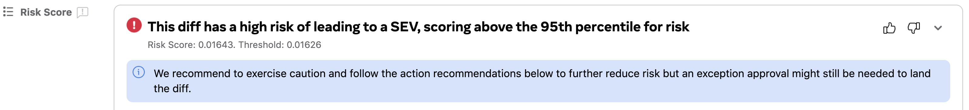
Figure 1: Showing the Risk in the Phabricator UI

The developer can wait until the code freeze is over and then land their diff. For example, if the code freeze starts on a Friday, the developer can wait until the following Monday morning to land their diff. This allows the developer to ensure that any issues or problems that may arise during the code freeze are addressed before their diff is landed. Additionally, waiting until after the code freeze is over ensures that the diff is not blocked from landing due to the increased risk threshold. In the event that the diff needs to land, there is an escalation process. There are a set of standard reasons that will escalate the diff to the managers that may accept the reason for the diff to land during the code freeze.

Figure 1 shows the information provided to the developers in the Phabricator UI, which includes the risk score of the diff, feedback mechanisms, informational section, reasons for the diff to be considered risky, and potential actions. The risk score is a value that represents the level of risk associated with the diff. The feedback mechanisms allow the developer to provide feedback on the usefulness of the diff risk score. The reasons for the diff to be considered risky are also listed, along with potential actions that the developer can take to reduce the risk score and land the diff successfully.

III Models

We examine three types of models: regression model, RoBERTa-based model, and LLMs.

III-A Regression Model

Table III shows the features used in one version of the the final model. For a logistic regression model the fitted model is simply a single vector multiplication of fitted coefficients and predictors, so the only hard part is to ensure that the values of the predictors are available in real time.

The large number of predictors (close to 100 were calculated based on academic literature and specific aspects of the way software development at Meta is structured – see Section II-A) and high correlations among them provide opportunity to select a single predictor from each of the fairly large correlated groups of predictors. Such clusters of predictors tend to be representing distinct phenomena that may increase the risk. For example, how diffuse the diff is and how much code it modifies, how much experience author had modifying the changed code previously, the properties of the modified files, such as programming language used, complexity of the code in the modified files, and external information such as prior history of being modified by a SEV causing diff or being used to implement highly critical service.

This process involves considerations on prioritizing predictors that are actionable and easy to explain to developers. Obviously, any constraints on predictor selection may affect model performance, so this careful manual selection process attempts to balance actionability, ease of understanding, and performance.

Table III shows features of the production model presented in the results section. It includes properties of the change, like how many files are modified, properties of the modified code, like lines of code changed or programming language, properties of the developer making the change like their experience and part of organization. More unusual predictors include an indicator of whether the code is a part of a critical service. Most important software services are classified according to their criticality and code executed as part of such services is then tagged according to that class. To fit the model and do historic performance analysis all measures are calculated as of time the diff was landed.

TABLE I: The features used in the logistic regression that is in production

Feature type	Feature used in Logistic Regression
Diff	$log$ of the added and deleted SLOC relative to size of file (ratio)
	New files created by the diff (boolean)
	Diff only creates new files (boolean)
Diffusion	$\log$ of the number of files in this diff
	$log$ of the number of authors that modified changed files
Criticality	Previous SEV in the file (boolean)
	Previous SEV in the folder (boolean)
	Is file involved in high-criticality service (boolean)
File	Total logical complexity of files touched in this diff
	Programming language (seven boolean indicators if at least one file in that language is modified)
Expertise	If the author is the original creator of the file
	Number of diffs previously landed by the author

TABLE II: The features fed to the LLMs during both training and inference for DRS

Feature type	Feature fed to the LLM
Diff Title	Title of the diff, typically a concise description of the code change in a few words
Test Plan	Commands (build, lint, tests) executed by the diff author to validate the code changes
Code changes	Filenames and the corresponding code changes in the standard unified diff (“unidiff”) format

III-B Why Large Language Models?

The underlying DRS model today is a logistic regression trained on diff metadata such as the diff, file, author and related features. One limitation of such simple models is that they do not understand any content based features, e.g., diff code, summary test plan etc., which arguably can contain the highest signal of diff risk. For instance, a diff that only adds comments to a file can never cause a SEV, but could be flagged by the model because it touches the same file as a previous SEV-causing diff. On the other hand, a particular code pattern that consistently causes a SEV could be missed by the model because of its inability to understand code changes.

Recently, LLMs have been proven to be effective in understanding and generating textual and code content. As a result they have been widely adopted to help improve software engineering productivity [29, 26, 30, 31]

Large language models (or LLMs) in recent years have been proven to be efficient in code understanding, improvement and generation, thus starting to be widely adopted to help improve software engineering efficiency[1,2]. We would like to leverage LLMs to understand the code change when doing diff risk score analysis to improve the accuracy of diff risk score, boosting engineering productivity by highlighting and providing suggestions for engineers.

LLMs also eliminate the potentially expensive feature engineering that is needed by simpler models such as logistic regression. For instance, when dealing with code, LLMs do not need to be fed hand-curated features about what language the code is in, how large it is, whether it is a comment, and so on. They can automatically learn these features internally as part of their training, albeit not human interpretable. Table II lists the textual and code features from a diff that are fed to the LLMs for both training and inference for risk prediction.

III-C StarBERT model

StarBERT is a RoBERTa-based model for understanding semantics of various artifacts across Meta ’s internal platform [13]. It can be used for several different purposes, including classification, embedding generation, score computation (regression) and more [14, 15, 16].

At the core of StarBERT platform are the pretrained models. The representations learned by these models are generic and transfer to downstream tasks of platform users through fine-tuning. Transfer learning provides substantial benefits to user teams by (1) requiring much smaller labeled datasets, (2) immediate benefit of base-line performance out of the box, (3) simplifying feature selection and (4) considerably faster model iterations. Pretraining is essential to save on the research and development that goes into model building and selection as well as enable impact that is otherwise not possible.

To fine tune the model for a specific task such as computing the risk score of a diff, labeled/annotated code diffs are used to inject task-specific inductive bias into the pre-trained model. The goal is to train (finetune) the model to accurately determine whether an unseen diff is likely to cause a SEV.

III-D Generative LLMs

The state-of-the-art generative LLMs of today have been effective at powering several software engineering tasks, ranging from code completion [22, 24], test generation [23], to code review [26]. These models are based on a “foundation model” that is pre-trained on internet-scale data (billions of tokens) on a simple generic task, i.e., next token prediction. They are then prompted as-is or fine-tuned further on domain specific data to elicit increased performance on a specific task.

CodeLlama [27] is such an AI model built on top of Meta GenAI’s Llama 2 [32], fine-tuned for generating and discussing code. Essentially, CodeLlama features enhanced coding capabilities. It can generate code and natural language about code, from both code and natural language prompts (e.g., “Write me a function that outputs the Fibonacci sequence”). It can also be used for code completion and debugging. It supports many of the most popular programming languages used today.

For this work, we considered two models built on top of CodeLlama.

III-D1 iCodeLlama

iCodeLlama is a Meta-internal model that we have developed by further pre-training CodeLlama on Meta’s proprietary code base, including code from our monorepo, natural language comments appearing inline, and other code-related documentation. It exhibits similar capabilities as CodeLlama but on Meta’s internal contexts. iCodeLlama-7B has been used to power Meta’s code completion system, CodeCompose [24, 25].

III-D2 iDiffLlama

iDiffLlama is also based on CodeLlama, but in addition to pre-training on code and natural language, it is also pre-trained on internal diffs, i.e., code changes. This makes the model “change-aware” as it understands the nuances of not just static code, but also the evolution of code through changes. Particularly, diffs represent an intent by a developer to commit their changes to the monorepo. iDiffLlama captures that intent through learning the relationship between a diff’s title, summary, test plan and the corresponding code changes.

III-E Using Generative LLMs for classification

The first question to answer when using today’s LLMs (iCodeLlama or iDiffLlama) for a problem like DRS is, can generative models be used for classification problems? They are designed for generating text or code and having conversations rather than classifying an input into categories.

One simple way to leverage a GenAI model for classification is through prompting (0-shot or few-shot). While this approach works for other applications, there are two problems with it particular to DRS:

• The model needs to provide a risk score rather than a binary label, as the score is used for ranking. Prompting the model to output a score is quite tedious as the model has to generate a numerical score token by token. It is also unreliable, as the model does not have a universal view of risk and may generate uncalibrated scores across different examples.

• The input to DRS is not a simple piece of text but a heavyweight diff which often occupies a significant portion of the context window, making few-shot with current generative models infeasible. DRS is also an inherently hard problem due to its needle-in-the-haystack nature, and it is difficult to provide sufficiently balanced examples for few-shot learning.

Instead, we explored two methods for using LLMs for classification: embeddings from foundation model, and risk alignment.

III-E1 Embeddings from foundation model

The idea here is to extract the relevant features from a given diff, embed the features using the pre-trained foundation LLM, and use those embeddings along with the labeled DRS data to train an off-the-shelf classifier such as an MLP. The pipeline is illustrated in Figure 2.

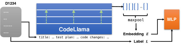
Figure 2: Pipeline: Embeddings from foundation model. A model forward pass is run on the input diff, and hidden states from the final Transformer layer are aggregated via maxpool to form the diff’s embedding $E$. An external classifier is then trained on the embeddings and labeled DRS data.

To compute embeddings for an input diff, we do a single forward pass on the input and aggregate the hidden states in the final layer of the Transformer model. We experimented with meanpool and maxpool, and found maxpool to work slightly better. One advantage of this approach is that it makes it easier to integrate the embeddings with the current logistic model trained on other metadata features.

III-E2 Risk alignment

In this approach (depicted in Figure 3), we run a typical supervised fine-tuning (SFT) phase on the pre-trained LLM using labeled DRS data. In order to transform the classification problem into a generative task, we use special markers [DRS][/DRS] to annotate the input, append the label (0 or 1) to the end, and train the model to “generate” the label token.

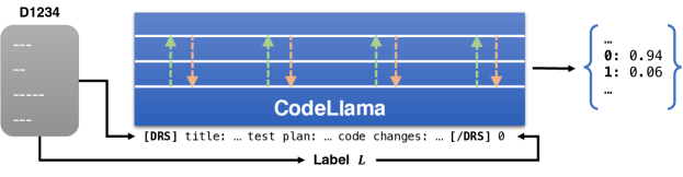
Figure 3: Pipeline: Risk alignment. The LLM undergoes supervised fine-tuning (SFT) on labeled DRS data, where each diff is annotated with special tokens [DRS][/DRS] that denote the model to predict risk. The LLM is trained to generate the label token 0 or 1 appended to the end of the input. During inference, the risk score is computed based on the token probabilities of the labels 0 and 1.

During inference, we can query the model to generate the label token. To get the risk score rather than just the label, we extract the probability of the label tokens “0” and “1” from the next token distribution. If the model is aligned well, all other tokens in the model’s vocabulary should have close to zero probability of being generated.

The advantage of this approach is that it allows the LLM to backpropagate and learn the nuances of diff risk, i.e., makes it “risk-aligned”, rather than serving untuned embeddings that only capture general properties of diffs. However, this requires a computationally expensive fine-tuning of the LLM and deployment of this specialized model.

IV Evaluation Method and Data

To ensure a fair comparison of different models for Diff Risk Scoring (DRS), we use the same dataset and splits across all models. We split our data chronologically (by diff closed date) into training, validation, and testing sets. This approach offers a more realistic split compared to random sampling, as it better reflects the temporal nature of the data.

Although Meta has a monorepo, we scoped our experiment and data to a particular organization’s diffs within the company. This allows us to test the model’s generalization capability (see Section V), as well as focus engineering efforts on deployment within the pilot organization at Meta.

Our testing data consists of $181052$ regular diffs and $305$ SEVs. By using a chronological split, we can evaluate the models’ performance on unseen data that was not used during training or validation. This allows us to better assess their ability to generalize to new, unseen data in real-world scenarios.

TABLE III: Data splits

	diff closing data from	diff closing data to	sample size	SEV count/rate
Training	2022-01-01	2023-05-04	855282	1981 (0.23%)
Validation	2023-05-05	2023-05-06	120967	214 (0.18%)
Testing	2023-07-01	2023-10-02	181052	305 (0.17%)

Dealing with skewed data. When either training an external classifier or aligning the LLM for risk prediction, there is an extreme imbalance in the labeled data, as SEV-causing diffs account for less than 1% of all diffs (see Table III). To deal with this imbalance we resampled the examples in the training data to arrive at a 5:1 negative-positive class ratio. We did this only for the training data to ensure that the model does not regress to overwhelmingly predicting the majority class. We did not modify the validation and testing data in order to preserve the real world distribution. We then froze the resampled training data and used it for all models.

For the dataset we select the top g riskiest diffs from each model, and determine as outcome what percentage of SEVs that would be captured. We use the current production gating levels of 5% (weekend), 10% yellow or intermediate, and 50% red or high.

V Results

TABLE IV: The percentage of captured SEVs by model as well as the percentage increase relative to the current project logistic regression model

Model	Weekend (g = 5%)		Yellow (g = 10%)		Red (g = 50%)
	SEVs Captured	vs Regression	% SEVs Captured	vs Regression	% SEVs Captured	vs Regression
Logistic Regression	18.7 %	$-$ $\times$	27.9 %	$-$ $\times$	84.6 %	$-$ $\times$
StarBERT	11.5 %	0.61 $\times$	23.6 %	0.85 $\times$	68.9 %	0.81 $\times$
iCodeLlama-34B	10.8 %	0.58 $\times$	18.0 %	0.65 $\times$	69.2 %	0.82 $\times$
iCodeLlama-34B risk aligned	23.6 %	1.26 $\times$	35.7 %	1.28 $\times$	83.0 %	0.98 $\times$
iDiffLlama-13B	12.1 %	0.65 $\times$	22.6 %	0.81 $\times$	75.7 %	0.90 $\times$
iDiffLlama-13B risk aligned	26.2 %	1.40 $\times$	42.3 %	1.52 $\times$	88.5 %	1.05 $\times$

RA 1. Logistic Regression

How well does the current model capture SEVs?

For production use at scale, we need a simple model and features that can be calculated across thousands of engineers and diffs. As we discussed in the model development, see Section III-A, we reviewed the literature on defect modelling and selected the represented set of features shown in Table III.

In Table IV, we see that our baseline regression model captures 18.7%, 27.9%, and 84.6% of SEVs while respectively gating the top 5% (weekend), 10% (yellow), and 50% (red) of risky diffs. This regression model has been used in production for more than 9 months.

RA 2. StarBERT

How well does a RoBERTa-based model capture SEVs?

StarBERT is a RoBERTa-based [13] large language model. For the purpose of gating during code freeze, labeled/annotated code diffs are used to inject task-specific inductive bias into the pre-trained model. The goal is to train (finetune) the model to accurately determine whether an unseen diff is likely to cause a SEV. The model develop in fully described in Section III-C.

In Table IV, we see the StarBERT model only captures 0.61$\times$, 0.85$\times$, and 0.81$\times$ as many SEVs as the logistic regression for the weekend, yellow, and red gating zones, respectively. Clearly the RoBERTa-based model cannot replace the logistic regression for production purposes.

RA 3. Generative LLMs

For generative LLMs, we pick the two models. Specifically, we take iCodeLlama-34B and iDiffLlama-13B, having 34B and 13B parameters, respectively. The full details on the model development can be found in Section III-D.

RA 3a. FM LLMs

How well does the foundation pre-trained model capture SEVs?

We use the embedding in the from the iCodeLlama-34B and iDiffLlama-13B and use a classifier to determine the DRS risk score. The method is described in Section III-E1 and the pipeline is shown in Figure 2. We trained an external 3-layer MLP classifier on the embeddings consisting of $(100,150,50)$ hidden units, respectively.

In Table IV, we see that without aligning for risk, the iCodeLlama-34B model only captures 0.58$\times$, 0.65$\times$, and 0.82$\times$ as many SEVs as the logistic regression for the weekend, yellow, and red gating zones, respectively. The corresponding numbers for iDiffLlama-13B are 0.65$\times$, 0.81$\times$, and 0.90$\times$. This shows that unaligned foundation LLMs are not effective at capturing SEVs.

RA 3b. Risk aligned LLMs

Does aligning the LLM towards risk prediction allow it capture more SEVs?

We saw that using the embeddings with an MLP was ineffective. We fine-tune the iCodeLlama-34B and iDiffLlama-13B by running one epoch on the training data with an effective batch size of 64. The training was conducted on a cluster of 64 Nvidia A100 GPUs, and took around 2-4 hours to complete depending on the size of the LLM. The full methodology to make the LLMs risk aligned is described in Section III-E2 and the pipeline is shown in Figure 3.

In Table IV, when iCodeLlama-34B is risk aligned it captures 1.26$\times$, 1.28$\times$, and 0.98$\times$ as many SEVs as the logistic regression for the weekend, yellow, and red gating zones, respectively. The corresponding number for iDiffLlama-13B are 1.40$\times$, 1.52$\times$, 1.05$\times$.

An interesting observation here is that while both risk aligned models outperform the baseline logistic regression, iDiffLlama-13B outperforms iCodeLlama-34B despite being a smaller model. This reveals that change-aware (diff) pre-training adds significant value to an LLM’s performance on predicting diff risk. This makes sense as DRS is essentially a diff related problem. Thus, we have arrived at a new state-of-the-art for diff risk prediction at Meta, with the change-aware risk-aligned model iDiffLlama-13B.

3c. Generalizability

How well does the best performing research approach generalize beyond its organization?

In order to test the model’s generalizability, we used the risk aligned iDiffLlama-13B to predict the diff risk for diffs in another organization under Meta. We ensured that there is no overlap between diffs that land in the two organizations’ part of the code base. As before, we compared the model to an existing logistic regression model used in the other organization.

Out of 160 SEVs the logistic regression model was able to capture 11.9%, 26.3% and 84.4% of SEVs at the three gating thresholds of 5%, 10% and 50%, respectively. However, iDiffLlama-13B was able to capture 21.9%, 39.4%, and 88.8% of SEVs at the same thresholds, translating to a 1.84$\times$, 1.5$\times$, and 1.05$\times$ improvement over the baseline. This shows that LLMs are effective at generalizing beyond their training domain for predicting diff risk.

VI Threats to Validity

VI-A Generalizability

One potential threat to the generalizability of our findings is the limited scope of our dataset. Our study was conducted using data from a single company, which may not be representative of all software development scenarios. The specific tools, processes, and culture of our company may have influenced the results of our study, and other companies may have different factors that impact their release engineering decisions. Therefore, it is unclear whether our findings can be generalized to other contexts.

VI-B Construct Validity

Another potential threat to validity is construct validity. Our study focused on diff risk scoring for SEV prevention only, and did not consider other factors that may impact release engineering decisions, such as business value or user feedback. Therefore, our approach may not fully capture the complexity of the problem and may not be suitable for all release engineering scenarios. Additionally, our models were trained on historical data, which may not be representative of future software development scenarios. Therefore, the performance of our models may degrade over time and require periodic retraining.

VI-C Internal Validity

Finally, there are potential threats to internal validity in our study. One potential threat is the evaluation metric used to assess the performance of our models. We evaluated our models based on a single metric, SEV capture rate, which may not fully capture the complexity of the problem. Other metrics, such as the ultimate goal of reducing the number and impact of SEVs and minimizing disruptions to developer productivity from gating, may provide additional insights into the effectiveness of our approach. Another potential threat is the possibility of unmeasured confounding variables that may have impacted our results. For example, there may be other factors that influence the likelihood of a diff causing a SEV, such as code quality or team dynamics, that were not captured in our analysis.

VII Discussion and Literature

VII-A Release Engineering

Release engineering is a discipline of software engineering that focus on creating pipelines that takes source code and turns it into a final product that is ready for release. This includes compiling, packaging, testing, and signing the code [33]. The goal of release engineering is to ensure that the pipeline is efficient and reliable, so that products can be delivered to customers quickly and with high quality. This is especially important for companies like Meta, providing services to millions of users, as they need to be able to deliver updates to their customers in a timely manner. Code freeze, the main focus of this paper, is a common practice during which no changes are allowed to be made to the codebase, in order to ensure stability and prevent any issues during critical periods such as holidays or major events.

The models we discussed in the paper aim at relaxing the code freeze periods, this way allowing users to land diffs that are considered not to harm the stability of the current release. This is, a move towards a code chill, which is a step in moving away from a hard/strict code freeze, as it allows teams to deploy important changes more freely and gives them the autonomy – and responsibility – to make the call on whether a deployment is important enough to risk deploying. To help teams have that autonomy, and responsibility, we are equipping the teams at Meta with a quantification of the diff risk score of their diffs.

The models presented in the paper aim to reduce the strictness of code freeze periods, enabling developers to land diffs that are deemed safe for the current release (that is, do not compromise the stability of the current release). This approach represents a shift towards a “code chill,” which is a step towards relaxing strict code freeze policies and allows teams to deploy changes more easily while assuming responsibility for their decisions. To support this autonomy and accountability, we are providing Meta teams with a quantitative assessment of the risk associated with their diffs.

VII-B Defect Prediction Models

Code quality is one of the pillars of software engineering and statistical models attempting to predict software defects have been developed in the previous century [5, 6]. While traditional defect prediction models focus on identifying which files will have defects, just-in-time defect prediction models [7, 9] attempt to predict which change (diff) will cause a problem. Both fields are extremely mature (see systematic surveys of recent work in, e.g.,,  [12] for just-in-time prediction,  [34] for the more recent development of application of deep learning methods).

One aspect that distinguishes our effort from almost all prior work is the accuracy of identifying SEVs causing diffs. At Meta, all SEVs undergo a rigorous review process and the trigger (cause) is identified. While sometimes SEV is caused by hardware failures or network outages, often the cause is a software change (diff). Virtually all published work uses rather noisy estimates of which diff caused the problem based on information from issue-fixing diffs, while in our case the data is manually derived by area experts.

VII-C Costs: Human vs. Machine

There is always a cost associated with training and deploying models. For the logistic regression model, the cost is in terms of human time involved in feature engineering, i.e., cleaning the data, curating and implementing features, determining best predictors, feature importance, etc. Whereas, the compute cost involved in training and deploying the model is relatively small. They can be trained on CPUs, and usually take in the order of minutes to complete.

On the other hand, LLMs require heavy compute power to operate. They require GPUs to train and deploy, and take in the order of hours or days to train. However, they completely eliminate the need to do any feature engineering. They are able to take in raw data and learn these (latent) features during their training. They also have a highly desirable property of transfer learning across training phases, as they are based on a powerful foundation model pre-trained on billions of tokens. These characteristics allow LLM-based solutions to follow simpler scaling laws, as data and compute become the only two requirements for scaling up.

VIII Future Work

We discuss two avenues of future work: (1) generative reasoning on why a diff may lead to a SEV (2) ensemble learning combining LLMs and regressions.

VIII-A LLM fine-tuning for generative reasoning

Generative reasoning is an alternative approach to classification. With an appropriate SFT phase, LLMs could potentially synthesize an answer of whether a diff is risky along with an explanation of why, in a purely generative manner. This method is used in the AI community to have LLMs adapt to specific problem domains, such as the work done in Microsoft Research [35]. On the other hand, SFT for generative reasoning than classification is a much longer term effort, owing to the following:

• It requires large investment to collect actual SEV reasoning traces and their root causes, rather than the label of whether the diff caused a SEV. Moreover, discussions around SEVs are multi-modal, involving a combination of natural language, code, screenshots or videos, and so on. Developing a multi-modal LLM capable of reasoning about SEVs is beyond the scope of this paper.

• Hallucinations are a major problem with generative reasoning, which would confuse the user even more if the LLM generated the wrong explanation. Mitigating hallucinations is still very early research, and the industry has little experience on this. There are existing efforts to optimize prompt engineering to mitigate hallucinations, which from our observation provides limited help.

VIII-B Ensembling LLM’s and Logistic Regression’s risk score

The diff, author, and file related features in the logistic regression model continue to be powerful and valuable predictors. Consequently, it is advantageous to ensemble the LLM and the logistic regression model. We incorporated the LLM score as an additional feature into the logistic regression model. During the inference process, an LLM score is initially obtained, followed by the computation of logistic regression. In instances where the LLM score is absent (due to timeout, etc.), we impute it as the mean.

Alternative ensemble strategies include:

• Utilizing the LLM embedding as input variables for logistic regression rather than the prediction score, which may encompass more comprehensive information.

• Implementing a weighted average of the LLM score and logistic regression score, where the weight is determined by maximizing precision/recall on the evaluation dataset.

• Considering the addition of features in logistic regression into the LLM, enabling the LLM to fully supplant the logistic regression model.

IX Conclusion

In conclusion, our study has demonstrated that the use of machine learning models can significantly improve the accuracy of diff risk scoring, which can help release engineers make more informed decisions about which diffs to gate. The logistic regression outperformed the RoBERTa-based models. However, the generative LLM models showed promising results, with the iDiffLlama-13B model capturing the most SEVs among all models tested.

The following are some highlights and learning worthy of note from our experiment:

• Our experiment answered the question of whether generative models can be suited for a classification problem like DRS. We validated using both the foundation models and risk aligned models for classification. Although expected, the results confirm that fine-tuning a model for a problem domain significantly boosts its performance compared to using a pre-trained model, i.e., risk aligned models outperformed pre-trained models across all metrics.

• Directly using the LLM for prediction performs better than using an external classifier trained on foundation LLM embeddings. This is likely due to the fact that there is loss of information when aggregating (pooling) hidden states for embeddings, and there is no self-attention in the external classifier when making the prediction.

• The change-aware model iDiffLlama-13B outperforms the general purpose code LLM iCodeLlama-34B, despite the former being a smaller model. This is due to it being a specialist model specifically trained to understand diff data in the form of patches.

These findings highlight the potential of machine learning models to enhance the efficiency and safety of the software development process. Future work includes further refinement of the models and exploration of additional features to incorporate into the models.

References

- [1] M. T. Rahman, L.-P. Querel, P. C. Rigby, and B. Adams, “Feature toggles: Practitioner practices and a case study,” in Proceedings of the 13th International Conference on Mining Software Repositories, ser. MSR ’16. New York, NY, USA: Association for Computing Machinery, 2016, p. 201–211. [Online]. Available: https://doi.org/10.1145/2901739.2901745
- [2] C. Rossi, “Rapid release at massive scale,” Web site: https://engineering.fb.com/web/rapid-release-at-massive-scale, 2017.
- [3] A. Krutauz, T. Dey, P. C. Rigby, and A. Mockus, “Do code review measures explain the incidence of post-release defects?” vol. 25, no. 5. Springer, 2020, pp. 3323–3356.
- [4] S. R. Dalal and C. L. Mallows, “When should one stop testing software?” Journal of the American Statistical Association, vol. 83, no. 403, pp. 872–879, 1988.
- [5] J. D. Musa, A. Iannino, and K. Okumoto, Software Reliability: Measurement, Prediction, Application. McGraw-Hill Book Company, 1987, iSBN: 0-07-044093-X.
- [6] T. L. Graves, A. F. Karr, J. S. Marron, and H. Siy, “Predicting fault incidence using software change history,” IEEE Transactions on Software Engineering, vol. 26, no. 2, 2000.
- [7] A. Mockus and D. M. Weiss, “Predicting risk of software changes,” Bell Labs Technical Journal, vol. 5, no. 2, pp. 169–180, April–June 2000. [Online]. Available: papers/bltj13.pdf
- [8] N. Nagappan and T. Ball, “Use of relative code churn measures to predict system defect density,” in Proceedings of the 27th international conference on Software engineering, 2005, pp. 284–292.
- [9] Y. Kamei, E. Shihab, B. Adams, A. E. Hassan, A. Mockus, A. Sinha, and N. Ubayashi, “A large-scale empirical study of just-in-time quality assurance,” IEEE Transactions on Software Engineering, 2013. [Online]. Available: http://doi.ieeecomputersociety.org/10.1109/TSE.2012.70
- [10] J. Pachouly, S. Ahirrao, K. Kotecha, G. Selvachandran, and A. Abraham, “A systematic literature review on software defect prediction using artificial intelligence: Datasets, data validation methods, approaches, and tools,” Engineering Applications of Artificial Intelligence, vol. 111, p. 104773, 2022.
- [11] H. Keshavarz and M. Nagappan, “Apachejit: a large dataset for just-in-time defect prediction,” in Proceedings of the 19th International Conference on Mining Software Repositories, 2022, pp. 191–195.
- [12] Y. Zhao, K. Damevski, and H. Chen, “A systematic survey of just-in-time software defect prediction,” ACM Computing Surveys, vol. 55, no. 10, pp. 1–35, 2023.
- [13] M. Beller, H. Li, V. Nair, V. Murali, I. Ahmad, J. Cito, D. Carlson, A. Aye, and W. Dyer, “Learning to learn to predict performance regressions in production at Meta,” in 2023 IEEE/ACM International Conference on Automation of Software Test (AST). IEEE, 2023, pp. 56–67.
- [14] A. Karmakar and R. Robbes, “What do pre-trained code models know about code?” in 2021 36th IEEE/ACM International Conference on Automated Software Engineering (ASE). IEEE, 2021, pp. 1332–1336.
- [15] Z. Ding, H. Li, W. Shang, and T.-H. P. Chen, “Can pre-trained code embeddings improve model performance? revisiting the use of code embeddings in software engineering tasks,” Empirical Software Engineering, vol. 27, no. 3, p. 63, 2022.
- [16] X. Zhou, D. Han, and D. Lo, “Assessing generalizability of codebert,” in 2021 IEEE International Conference on Software Maintenance and Evolution (ICSME). IEEE, 2021, pp. 425–436.
- [17] A. Fan, B. Gokkaya, M. Harman, M. Lyubarskiy, S. Sengupta, S. Yoo, and J. M. Zhang, “Large language models for software engineering: Survey and open problems,” arXiv preprint arXiv:2310.03533, 2023.
- [18] C. Ebert and P. Louridas, “Generative ai for software practitioners,” IEEE Software, vol. 40, no. 4, pp. 30–38, 2023.
- [19] A. Ziegler, E. Kalliamvakou, X. A. Li, A. Rice, D. Rifkin, S. Simister, G. Sittampalam, and E. Aftandilian, “Measuring github copilot’s impact on productivity,” Communications of the ACM, vol. 67, no. 3, pp. 54–63, 2024.
- [20] B. Yetiştiren, I. Özsoy, M. Ayerdem, and E. Tüzün, “Evaluating the code quality of ai-assisted code generation tools: An empirical study on github copilot, amazon codewhisperer, and chatgpt,” arXiv preprint arXiv:2304.10778, 2023.
- [21] A. Hindle, E. T. Barr, M. Gabel, Z. Su, and P. Devanbu, “On the naturalness of software,” Communications of the ACM, vol. 59, no. 5, pp. 122–131, 2016.
- [22] (Accessed 2021) Github copilot. Github. [Online]. Available: https://github.com/features/copilot
- [23] M. Schäfer, S. Nadi, A. Eghbali, and F. Tip, “An empirical evaluation of using large language models for automated unit test generation,” 2023.
- [24] V. Murali, C. Maddila, I. Ahmad, M. Bolin, D. Cheng, N. Ghorbani, R. Fernandez, N. Nagappan, and P. C. Rigby, “Ai-assisted code authoring at scale: Fine-tuning, deploying, and mixed methods evaluation,” in Foundations of Software Engineering (FSE), 2024.
- [25] O. Dunay, D. Cheng, A. Tait, P. Thakkar, P. C. Rigby, A. Chiu, I. Ahmad, A. Ganesan, C. Maddila, V. Murali, A. Tayyebi, and N. Nagappan, “Multi-line ai-assisted code authoring,” 2024.
- [26] A. Frömmgen, J. Austin, P. Choy, N. Ghelani, L. Kharatyan, G. Surita, E. Khrapko, P. Lamblin, P.-A. Manzagol, M. Revaj, M. Tabachnyk, D. Tarlow, K. Villela, D. Zheng, S. Chandra, and P. Maniatis, “Resolving code review comments with machine learning,” in 2024 IEEE/ACM 46th International Conference on Software Engineering: Software Engineering in Practice (ICSE-SEIP), 2024.
- [27] B. Roziere, J. Gehring, F. Gloeckle, S. Sootla, I. Gat, X. E. Tan, Y. Adi, J. Liu, T. Remez, J. Rapin et al., “Code llama: Open foundation models for code,” arXiv preprint arXiv:2308.12950, 2023.
- [28] S. Haykin, Neural networks: a comprehensive foundation. Prentice Hall PTR, 1994.
- [29] N. Nguyen and S. Nadi, “An empirical evaluation of github copilot’s code suggestions,” in Proceedings of the 19th International Conference on Mining Software Repositories, 2022, pp. 1–5.
- [30] M. Schäfer, S. Nadi, A. Eghbali, and F. Tip, “An empirical evaluation of using large language models for automated unit test generation,” IEEE Transactions on Software Engineering, 2023.
- [31] ——, “Adaptive test generation using a large language model,” arXiv e-prints, pp. arXiv–2302, 2023.
- [32] H. Touvron, L. Martin, K. Stone, P. Albert, A. Almahairi, Y. Babaei, N. Bashlykov, S. Batra, P. Bhargava, S. Bhosale et al., “Llama 2: Open foundation and fine-tuned chat models,” arXiv preprint arXiv:2307.09288, 2023.
- [33] B. Adams, S. Bellomo, C. Bird, T. Marshall-Keim, F. Khomh, and K. Moir, “The practice and future of release engineering: A roundtable with three release engineers,” IEEE Software, vol. 32, no. 2, pp. 42–49, 2015.
- [34] Z. M. Zain, S. Sakri, and N. H. A. Ismail, “Application of deep learning in software defect prediction: Systematic literature review and meta-analysis,” Information and Software Technology, vol. 158, p. 107175, 2023.
- [35] T. Ahmed, S. Ghosh, C. Bansal, T. Zimmermann, X. Zhang, and S. Rajmohan, “Recommending root-cause and mitigation steps for cloud incidents using large language models,” in Proceedings of the 45th International Conference on Software Engineering, ser. ICSE ’23. IEEE Press, 2023, p. 1737–1749. [Online]. Available: https://doi.org/10.1109/ICSE48619.2023.00149