Losing Treewidth In The Presence Of Weights

Abstract

In the Weighted Treewidth-$\eta$ Deletion problem we are given a node-weighted graph $G$ and we look for a vertex subset $X$ of minimum weight such that the treewidth of $G-X$ is at most $\eta$. We show that Weighted Treewidth-$\eta$ Deletion admits a randomized polynomial-time constant-factor approximation algorithm for every fixed $\eta$. Our algorithm also works for the more general Weighted Planar $\mathcal{F}$-M-Deletion problem.

This work extends the results for unweighted graphs by [Fomin, Lokshtanov, Misra, Saurabh; FOCS ’12] and answers a question posed by [Agrawal, Lokshtanov, Misra, Saurabh, Zehavi; APPROX/RANDOM ’18] and [Kim, Lee, Thilikos; APPROX/RANDOM ’21]. The presented algorithm is based on a novel technique of random sampling of so-called protrusions.

1 Introduction

Let $\mathcal{H}$ be a class of graphs. A natural vertex deletion problem corresponding to $\mathcal{H}$ is defined as follows: given a graph $G$ find a set $X\subseteq V(G)$ of minimum size for which $G-X\in\mathcal{H}$. This captures numerous fundamental graph problems such as Vertex Cover, Feedback Vertex Set, or Vertex Planarization. Vertex deletion problems have been long studied from the perspective of approximation algorithms, starting from the classic 2-approximation for Vertex Cover [7, 59] from the 70s. It is known that for every non-trivial hereditary class $\mathcal{H}$ the corresponding vertex deletion problem is NP-hard and APX-hard [55] so the best we can hope for in polynomial time is a constant-factor approximation. Alike for Vertex Cover, this can be achieved for any class $\mathcal{H}$ characterized by a finite family of forbidden induced subgraphs via a linear programming relaxation (or sometimes by other means [38, 52, 60]). Lund and Yannakakis [55] conjectured in the early 90s that this condition in fact captures all vertex deletion problems admitting a constant-factor approximation. This was quickly disproved with a 2-approximation for Feedback Vertex Set [5, 10] as the class of acyclic graphs (i.e. forests) does not admit such a characterization. Later, Fujito [35] constructed an infinite family of counterexamples based on matroidal properties. Nowadays, we know several more interesting counterexamples: block graphs [1], 3-leaf power graphs [3], (proper) interval graphs [13, 68], ptolemaic graphs [4], and bounded-treewidth graphs [29, 37].

The landscape of positive results is grimmer when we consider weighted vertex deletion problems. Here, the graph $G$ is equipped with a weight function $w\colon V(G)\to\mathbb{R}^{+}$ and we ask for a vertex set $X\subseteq V(G)$ of minimum total weight for which $G-X\in\mathcal{H}$. The constant-factor approximations for Vertex Cover, Feedback Vertex Set, and for classes defined by a finite family of forbidden induced subgraphs were originally presented already in the weighted setting, but apart from that we are only aware of such algorithms for ptolemaic graphs [4], $\theta_{c}$-free graphs [27, 49] (a special case of bounded-treewidth graphs; explained shortly), and the matroidal classes introduced by Fujito [35].

Treewidth reduction and minor hitting.

The class of forests coincides with the class of graphs with treewidth one [18, §7]. Hence a natural generalization of (Weighted) Feedback Vertex Set is (Weighted) Treewidth-$\eta$ Deletion, a problem studied in the context of bidimensionality theory [21, 31, 33, 34] and satisfiability [6]. Here, we look for a minimum-weight treewidth-$\eta$ modulator, that is, a vertex set $X\subseteq V(G)$ for which the treewidth of $G-X$ is bounded by $\eta$.

Treewidth is closely related to the theory of graph minors (see Section 3 for definitions). Since the graph property “treewidth at most $\eta$” is closed under taking minors, Robertson and Seymour’s Theorem implies that it can be characterized by a finite family of forbidden minors [63]. In addition, a minor-closed graph class has bounded treewidth if and only if at least one of its forbidden minors is planar [61]. The treewidth bound is known to be polynomial in the size of this planar graph [17].

For a finite family of graphs $\mathcal{F}$, the (Weighted) $\mathcal{F}$-M-Deletion problem (also known as $\mathcal{F}$-Minor Cover) asks for a minimum-size (resp. minimum-weight) set $X\subseteq V(G)$ for which $G-X$ does not contain any graph $F\in\mathcal{F}$ as a minor. If the family $\mathcal{F}$ contains a planar graph, we speak of (Weighted) Planar $\mathcal{F}$-M-Deletion. Observe that Treewidth-$\eta$ Deletion is a special case of Planar $\mathcal{F}$-M-Deletion. This special case is paramount to understand the general case: if $X\subseteq V(G)$ is a solution to Planar $\mathcal{F}$-M-Deletion then $\mathrm{\textbf{tw}}(G-X)\leq\eta$ for some constant $\eta$ depending on $\mathcal{F}$. Hence if we were able to compute a constant-approximate treewidth-$\eta$ modulator $Y$, we could then solve the problem optimally on the bounded-treewidth graph $G-Y$, and output the union of both solutions.

Other examples of $\mathcal{F}$-M-Deletion include deletion problems into the classes of outerplanar graphs (for $\mathcal{F}=\{K_{4},K_{3,2}\}$), planar graphs (for $\mathcal{F}=\{K_{5},K_{3,3}\}$), or classes of bounded pathwidth/treedepth. Note that in the second case the family $\mathcal{F}$ does not contain a planar graph, which corresponds to the fact that the class of planar graphs has unbounded treewidth.

Approximating $\mathcal{F}$-M-Deletion.

In their seminal work, Fomin, Lokshtanov, Misra, and Saurabh [29] presented a randomized constant-factor approximation for every Planar $\mathcal{F}$-M-Deletion problem in the unweighted setting. Subsequently, Gupta, Lee, Li, Manurangsi, and Włodarczyk [37] gave a deterministic algorithm with explicit approximation factor $\mathcal{O}(\log\eta)$ where $\eta$ is the treewidth bound imposed by excluding the family $\mathcal{F}$. Obtaining a constant-factor approximation for any family $\mathcal{F}$ without a planar graph is wide open. This includes the Vertex Planarization problem ($\mathcal{F}=\{K_{5},K_{3,3}\}$) for which the best approximation factors are $\mathcal{O}_{\varepsilon}(\mathsf{opt}^{\varepsilon})$ in polynomial time, for any $\varepsilon>0$, and $\log^{\mathcal{O}(1)}(\mathsf{opt})$ in quasi-polynomial time [43, 45].

The current-best approximation algorithms for Weighted Planar $\mathcal{F}$-M-Deletion have factors $\mathcal{O}(\log^{1.5}|V(G)|)$ (randomized), $\mathcal{O}(\log^{2}|V(G)|)$ (deterministic) [2] and $\mathcal{O}(\log|V(G)|\log\log|V(G)|)$ for the edge-deletion version [6]. Apart from Weighted Feedback Vertex Set, the only other case known to admit a constant-factor approximation corresponds to $\mathcal{F}=\{\theta_{c}\}$ [49]. Beforehand, a specialized algorithm was given for $\mathcal{F}=\{\theta_{3}\}$ where the corresponding deletion problem was dubbed Weighted Diamond Hitting Set [27]. Apart from that, Weighted Planar $\mathcal{F}$-M-Deletion admits a PTAS on bounded-genus graphs and a QPTAS on $H$-minor-free graphs [33]. To the best of our knowledge, the existence of a polynomial-time constant-factor approximation for Weighted Planar $\mathcal{F}$-M-Deletion remains open even on $H$-minor-free graphs.

Protrusion replacement.

The results of Fomin et al. [29] are based on the powerful technique of protrusion replacement [26]. An $r$-protrusion in a graph $G$ is a vertex subset $A\subseteq V(G)$ for which $\mathrm{\textbf{tw}}(G[A])\leq r$ and $|\partial_{G}(A)|\leq r$, where $\partial_{G}(A)$ is the subset of vertices from $A$ that have neighbors outside $A$. The idea of protrusion replacement is to analyze the behavior of an $r$-protrusion with respect to the considered problem and replace it with an equivalent subgraph of constant size. Apart from constant-factor approximations, the same work spawned single-exponential FPT algorithms parameterized by the solution size (under some additional restriction) and polynomial kernelizations (using a more advanced concept of a near-protrusion). For other applications of this technique, see e.g., [9, 12, 32, 43, 54].

The caveat of protrusion replacement is that in general it is only known to work for the unweighted problems. Kim, Lee, and Thilikos [49] designed a weighted variant of this technique for the special case of Weighted Planar $\mathcal{F}$-M-Deletion with $\mathcal{F}=\{\theta_{c}\}$. They suggested a roadmap to achieve a constant-factor approximation for the general case, concluding that “($\dots$) the most challenging step is to design a weighted protrusion replacer”.

We remark that the techniques used by Gupta et al. [37] in their constant-factor approximation for Planar $\mathcal{F}$-M-Deletion also fall short to process weighted graphs. Their algorithm repeatedly improves a solution $X$ by removing a small vertex set $Y$ to reduce the number of $X$-vertices in each connected component to $\mathcal{O}_{\mathcal{F}}(1)$. The argument ensuring the existence of such a set $Y$ relies on the properties of separators in a bounded-treewidth graph and breaks down when we replace “small” with “of small weight”.

FPT algorithms for weighted problems.

Apart from approximation, $\mathcal{F}$-M-Deletion has been studied extensively from the perspective of fixed-parameter tractability (FPT) [15, 20, 25, 42, 44, 50, 51, 53, 58, 65]. It is known that every Planar $\mathcal{F}$-M-Deletion problem can be solved in time $2^{\mathcal{O}_{\mathcal{F}}(k)}\cdot n^{\mathcal{O}(1)}$ where $k$ stands for the solution size [48]. Such a single-exponential parameter dependency is best possible under the Exponential Time Hypothesis already for Vertex Cover [39].

We will consider parameterized algorithms for weighted problems under the parameterization by the solution size $k$. More precisely, we look for a solution of minimum weight among those on at most $k$ vertices, called a $k$-optimal solution (see, e.g., [19, 24, 30, 46, 47, 56, 67]). Observe that the treewidth of a solvable instance of Weighted Planar $\mathcal{F}$-M-Deletion cannot exceed $k+\mathcal{O}_{\mathcal{F}}(1)$. Therefore, we can find a solution in time $2^{\mathcal{O}_{\mathcal{F}}(k\log k)}\cdot n^{\mathcal{O}(1)}$ via dynamic programming on a tree decomposition [9] (see [65, §7] for a discussion on treating weights). A single-exponential FPT algorithm is known for Weighted Feedback Vertex Set [1, 14]. Although we are not aware of any more general results, it is plausible that the techniques developed by Kim et al. [48] can be adapted to solve general Weighted Planar $\mathcal{F}$-M-Deletion in single-exponential time [64].

1.1 Our results

Our main conceptual message is that the need to design a weighted counterpart of the protrusion replacement technique can be circumvented. Instead, our algorithms are based on a new structural result about protrusions and treewidth modulators. We say that a non-empty family of $r$-protrusions $\mathcal{P}$ in $G$ forms an $(\eta,r,c)$-modulator hitting family if for every treewidth-$\eta$ modulator $X$ in $G$ at least $|\mathcal{P}|\,/\,c$ sets in $\mathcal{P}$ have a non-empty intersection with $X$.

Theorem 1.1.

For each $\eta>0$, every graph $G$ with $\mathrm{\textbf{tw}}(G)>\eta$ has an $\left(\eta,\mathcal{O}(\eta),2^{\mathcal{O}(\eta)}\right)$-modulator hitting family $\mathcal{P}$ of size $|V(G)|^{\mathcal{O}(\eta)}$. Furthermore, $\mathcal{P}$ can be constructed in time $|V(G)|^{\mathcal{O}(\eta)}$.

Equipped with a modulator hitting family $\mathcal{P}$ we can randomly sample an $\mathcal{O}(\eta)$-protrusion $A\in\mathcal{P}$ and then guess a piece of an optimal solution $X\cap A$ by considering $\mathcal{O}_{\eta}(1)$ options. The concrete choice of the probability distribution will be adjusted to specific applications.

This strategy bears some resemblance to random sampling of important separators [18, §8] used in the FPT algorithm for Multicut by Marx and Razgon [57]. Moreover, the proof of Theorem 1.1 also involves important separators and structures somewhat similar to important clusters from [57]. We remark however that the setups of these two techniques are disparate when it comes to the separator size (constant vs. parameter), the desired subset property (bounded treewidth vs. disjointedness with a given set) and the objective (intersect a solution vs. cover vertices that are in some sense irrelevant). Theorem 1.1 can also be compared to the algorithm by Fomin el al. [28] that involves random sampling of low-treewidth subgraphs in an apex-minor-free graph to cover an unknown small connected vertex set. That construction however relies on totally different techniques.

Our new tool enables us to design a first constant-factor approximation for Weighted Planar $\mathcal{F}$-M-Deletion, extending the results by Fomin et al. [29] and Gupta et al. [37] to the weighted realm. This resolves an open problem by Agrawal et al. [2] and Kim et al. [49]. In the statement below, $\eta(\mathcal{F})$ denotes the treewidth bound for the class of graphs excluding all $F\in\mathcal{F}$ as minors.

Theorem 1.2.

Let $\mathcal{F}$ be a finite family of graphs containing a planar graph. The Weighted $\mathcal{F}$-M-Deletion problem admits a randomized constant-factor approximation algorithm with running time $\mathcal{O}_{\mathcal{F}}\left(|V(G)|^{\mathcal{O}(\eta(\mathcal{F}))}\right)$.

Notably, all the known approximation algorithms for Weighted Planar $\mathcal{F}$-M-Deletion [2, 6, 33] and its special cases [5, 10, 27, 35, 49] rely on LP techniques whereas our algorithm is purely combinatorial. In particular, we do not follow the roadmap suggested by Kim et al. [49]. Circumventing protrusion replacement helps us avoid another issue troubling that technique, namely non-constructivity. Instead, our treatment of protrusions relies on explicit bounds on the sizes of minimal representative boundaried graphs in a certain equivalence relation by Baste, Sau, and Thilikos [9]. The values of the approximation factor and the constant hidden in the $\mathcal{O}_{\mathcal{F}}$-notation can be retraced from that work but they are at least double-exponential in $\eta(\mathcal{F})$.

As another application of Theorem 1.1, we present a single-exponential FPT algorithm for Weighted Planar $\mathcal{F}$-M-Deletion parameterized by the solution size $k$. As noted before, such a result could possibly be achieved by combining the protrusion decomposition by Kim et at. [48] with the exhaustive families described in Section 5, without using Theorem 1.1. Nevertheless, we include it as an illustration of versatility of our approach.

Theorem 1.3.

Let $\mathcal{F}$ be a finite family of graphs containing a planar graph. A $k$-optimal solution to Weighted $\mathcal{F}$-M-Deletion can be computed in randomized time $2^{\mathcal{O}_{\mathcal{F}}(k)}\cdot|V(G)|^{\mathcal{O}(\eta(\mathcal{F}))}$.

This algorithm returns a $k$-optimal solution with constant probability; otherwise it may either output a solution of larger weight or report a failure.

2 Techniques

We will now discuss how Theorem 1.1 facilitates designing approximation algorithms and compare our techniques to the previous works.

Protrusion replacement.

The starting point is the following randomized algorithm for unweighted Feedback Vertex Set. First, we can perform a simple preprocessing to remove vertices of degree 1 and 2. Then the number of edges in an $n$-vertex graph $G$ is at least $\frac{3n}{2}$. But when $X$ is a feedback vertex set then $G-X$ is a forest, which can have at most $n-1$ edges. Therefore at least $\frac{1}{3}$-fraction of edges is incident to $X$. We can thus sample a random edge and remove one of its endpoints, also chosen at random. The expected number of steps before we hit a vertex from $X$ is at most 6 so this algorithm yields 6-approximation in expectation.

Fomin et al. [29] invented a far-reaching generalization of this idea for the case when $X$ is a treewidth-$\eta$ modulator, i.e., $\mathrm{\textbf{tw}}(G-X)\leq\eta$ for some constant $\eta\in\mathbb{N}$. Their preprocessing procedure does not merely remove vertices of low degree but it detects and simplifies $r$-protrusions. A simple yet crucial observation is that the subgraph $G-X$ can be covered by $\mathcal{O}(|N(X)|)$ many $r$-protrusions for $r=2\eta+2$. Hence if we could only ensure that each $r$-protrusion has size $\mathcal{O}_{r}(1)$ then again a constant fraction of edges would be incident to $X$ and we could apply the same argument as above. This is what protrusion replacement is about: given an $r$-protrusion $A$ we would like to perform a “surgery” on $G$ to replace $G[A]$ with a subgraph of size $\mathcal{O}_{r}(1)$ that exhibits the same behavior.

The property of “being $\mathcal{F}$-minor-free” (as well as “having bounded treewidth”) can be expressed in counting monadic second-order (CMSO) logic. For such graph properties, Courcelle’s Theorem [12, Lemma 3.2] guarantees that subgraphs of constant-size boundary can be divided into a constant number of equivalence classes and replacing a subgraph with an equivalent one does not affect the property in question. But this is not enough as we do not know which vertices from such a subgraph are being removed by a solution. Protrusion replacement relies crucially on the observation that it is cheap to take into the solution the entire boundary of an $r$-protrusion. For a broad spectrum of problems this property (formalized as strong monotonicity [12, 29]) implies that the difference in cost between any two solutions over an $r$-protrusion is bounded by $\mathcal{O}_{r}(1)$. Consequently, there may be only finitely many non-equivalent “behaviors” of an $r$-protrusion. For each such equivalence class there is some $r$-protrusion of minimal size and it can be safely used as a replacement. Then the maximal size of such a replacement is some (implicit) function of $r$.

This technique breaks down for weighted graphs because it is no longer true that removing the boundary of an $r$-protrusion is cheap. Here, it is unclear whether the number of different “behaviors” can be bounded in terms of $r$ alone.

Sampling with weights.

Before we deal with weighted protrusions, let us sketch how to adapt the algorithm for Feedback Vertex Set to the weighted setting. First, we can still safely remove vertices of degree 1. Even though we cannot remove all vertices of degree 2, we can preprocess the graph to ensure that each such vertex is adjacent to higher degree vertices. After such preprocessing the number of edges is at least $\frac{5n}{4}$ and so at least $\frac{1}{5}$-fraction of edges is incident to the optimal feedback vertex set $X$. Observe that sampling a random endpoint of a random edge is equivalent to sampling a vertex proportionally to its degree so $\sum_{v\in X}\deg(v)\geq\frac{1}{10}\cdot\sum_{v\in V(G)}\deg(v)$. It is futile though to sample vertices according to the same distribution as before because the solution may consist of light-weighted vertices only and guessing just a few heavy vertices can blow up the solution weight. As we want to make the light-weighted vertices more preferable, we will sample a vertex $v$ of weight $w(v)$ with probability proportional to $\frac{\deg(v)}{w(v)}$. Let $W=\sum_{v\in V(G)}\frac{\deg(v)}{w(v)}$. Then the expected weight of the chosen vertex equals

$$\mathbb{E}\left[w(v)\right]=\sum_{v\in V(G)}w(v)\cdot\frac{\deg(v)}{w(v)\cdot W}=\sum_{v\in V(G)}\frac{\deg(v)}{W}.$$

On the other hand, the expected value of the revealed part of the solution equals

$$\mathbb{E}\left[w(v)\cdot 1_{v\in X}\right]=\sum_{v\in X}w(v)\cdot\frac{\deg(v)}{w(v)\cdot W}=\sum_{v\in X}\frac{\deg(v)}{W}\geq\frac{1}{10}\cdot\mathbb{E}\left[w(v)\right].$$

Even though the expected number of steps before we hit a vertex from $X$ might be large, the expected decrease of the optimum in each step is within a constant factor from the expected cost paid by the solution in this step. Such an algorithm can be still proven to yield 10-approximation via a martingale argument.

Sampling with protrusions.

The main obstacle remains how to deal with a situation when only a small fraction of edges is incident to a solution because of large protrusions. Let $X$ be a treewidth-$\eta$ modulator in $G$ of minimum weight and $r=\mathcal{O}(\eta)$. We exploit the structure of $G-X$ in a different way: since $G-X$ can be covered by few $r$-protrusions, we will sample a set $A$ from a family of $r$-protrusions that are in some sense maximal and hope that we pick a set $A$ that intersects $X$. This is exactly the idea formalized in Theorem 1.1. Next, we try to guess the set $X\cap A$ or some subset $Y\subseteq A$ which is “at least as good”. Even though the number of different “behaviors” of a weighted $r$-protrusion may be a priori unbounded, we can still use Courcelle’s Theorem to bound the number of different “types” of the partial solution $X\cap A$. Intuitively speaking, it is easier to enumerate “types of a partial solution” than “types of a protrusion” because in the latter case we need to understand all the behaviors of subgraphs attainable after removal of an unknown vertex set.

Suppose now that we are given an $r$-protrusion $A$ that is promised to intersect $X$. Using the “graph gluing” technique [40, 48], we enumerate a family $\mathcal{A}\subseteq 2^{A}$ of size $\mathcal{O}_{r}(1)$ such that either $X\cap A\in\mathcal{A}$ or there exists $Y\in\mathcal{A}$ for which $(X\setminus A)\cup Y$ is also an optimal solution. Next, we sample a random non-empty set from $\mathcal{A}$ in such a way that the probability of picking a particular $Y\in\mathcal{A}$ is proportional to $\frac{1}{w(Y)}$. By the same calculation as before, the expected value of the revealed part of a solution is within a multiplicative factor $|\mathcal{A}|=\mathcal{O}_{r}(1)$ from $\mathbb{E}\left[w(Y)\right]$, which is the key observation to design a constant-factor approximation. It is crucial that we can assume $X\cap A\neq\emptyset$ because the proposed sampling procedure makes sense only for sets $Y$ with a positive weight.

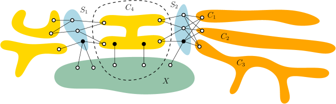
Figure 1: The set $X$ is a treewidth-$\eta$ modulator and $N(X)$ is represented by black discs. The blue sets $S_{1},S_{2}$ are two bags in a tree decomposition of $G-X$ that contain the marked vertices. The yellow and orange sets are the connected components of $G-(X\cup S_{1}\cup S_{2})$. For $i=1,2,3$ we have that $G[C_{i}]$ is connected, $\mathrm{\textbf{tw}}(G[C_{i}])\leq\eta$, and $N(C_{i})=S_{2}$, hence $(C_{i},S_{2})$ is a simple $\eta$-separation. The pair $(C_{1}\cup C_{2}\cup C_{3},\,S_{2})$ forms a semi-simple $\eta$-separation. The vertex set $C_{4}$ is enclosed by the dashed cycle. The simple $\eta$-separation $(C_{4},N(C_{4}))$ covers two edges outgoing from $X$ and so the set $N(C_{4})\setminus X$ has been marked. In the proof we take advantage of the fact that there can be no inclusion-wise maximal simple $\eta$-separation $(C,S)$ for which $C$ is contained in the yellow subset of $C_{4}$.

Main proof sketch.

Finally, we provide some intuition behind the proof of Theorem 1.1. It is more convenient for us not to work directly with protrusions but with pairs $(C,S)$ of vertex sets, where $N(C)\subseteq S$ and $\mathrm{\textbf{tw}}(G[C])+|S|$ is bounded. For technical reasons, we define an $\eta$-separation as such a pair in which $\mathrm{\textbf{tw}}(G[C])\leq\eta$ and $|S|\leq 2\eta+2$. Note that then $C\cup S$ forms a $(3\eta+2)$-protrusion. We call an $\eta$-separation simple when $G[C]$ is connected and $S=N(C)$.

We enumerate the family of inclusion-wise maximal simple $\eta$-separations. Since a bounded-treewidth subgraph may contain a large subfamily of such pairs $(C_{i},S_{i})$ for which $S_{i}$ coincide (see Figure 1), we need to merge such a subfamily into a single $\eta$-separation, that is called semi-simple. These structures can be compared to important clusters from the work [57]. Next, we would like every edge in the graph to be covered by some $\eta$-separation in the family, so if some edge $uv$ has not been covered so far, we insert the pair $(\emptyset,\{u,v\})$ to the family. Note that this forms a valid $\eta$-separation for any $\eta\geq 1$. Let $\mathcal{S}$ denote the family constructed according to this procedure.

Consider an unknown treewidth-$\eta$ modulator $X$ is $G$ and let $\mathcal{S}^{-}_{X}\subseteq\mathcal{S}$ denote the subset of those pairs $(C,S)$ for which $X\cap(C\cup S)=\emptyset$. Our goal is to show that $|\mathcal{S}^{-}_{X}|\leq\alpha\cdot|\mathcal{S}|$ for some $\alpha(\eta)<1$. First, for simplicity, assume that for every edge $uv$ outgoing from $X$ the pair $(\emptyset,\{u,v\})$ belongs to $\mathcal{S}$. Then it suffices to prove that the size of $\mathcal{S}^{-}_{X}$ is bounded by $\mathcal{O}(|N(X)|)$. This can be done using known techniques by analyzing a tree decomposition of $G-X$. However, the assumption above is clearly unrealistic because we do not know the set $E(X,V(G)\setminus X)$ and in general we cannot insert into $\mathcal{S}$ pairs $(\emptyset,\{u,v\})$ covered by larger $\eta$-separations as we want to keep the number of such pairs in $\mathcal{S}^{-}_{X}$ bounded.

The problematic case occurs when there is some $(C,S)\in\mathcal{S}$ that covers many edges outgoing from $X$ and so the comparison to $|N(X)|$ is no longer meaningful. Our strategy is to mark the vertices of $G-X$ that appear as $S$-vertices in some $(C,S)\in\mathcal{S}$ covering an edge $e\in E(X,V(G)\setminus X)$. We show that in fact the size of $\mathcal{S}^{-}_{X}$ is proportional to the number of marked vertices, which is bounded by $\mathcal{O}(|\mathcal{S}\setminus\mathcal{S}^{-}_{X}|)$. The proof is based on a case analysis inspecting the relative location of $(C,S)\in\mathcal{S}^{-}_{X}$ with respect to the marked set. We employ a win-win argument: in the problematic case the existence of a large simple $\eta$-separation covering many edges in $E(X,V(G)\setminus X)$ implies that a large piece of $G-X$ cannot contain simple $\eta$-separations that are inclusion-wise maximal (see Figure 1). These arguments allow us to bound the number of pairs $(C,S)\in\mathcal{S}^{-}_{X}$ for which $C$ is disjoint from the marked set. To handle the remaining pairs, we make a connection between simple $\eta$-separations and important separators. A key observation is that when $(C,S)$ is an inclusion-wise maximal simple $\eta$-separation with $X\cap(C\cup S)=\emptyset$ and $v\in C$ then $S$ forms an important $(v,X)$-separator. The number of such separators of size $\leq 2\eta+2$ is bounded by a function of $\eta$ for each marked vertex $v\in V(G-X)$ which results in the claimed bound.

3 Preliminaries

Graph notation.

We consider simple undirected graphs without self-loops. We follow the standard graph terminology from Diestel’s book [22] and here we only list the most important notation. For a vertex subset $A\subseteq V(G)$ we denote by $N_{G}(A)$ the open neighborhood of $A$, that is, the set of vertices from $V(G)\setminus A$ that have a neighbor in $A$. The closed neighborhood $N_{G}[A]$ is defined as $A\cup N_{G}(A)$. We sometimes omit the subscript when $G$ is clear from context. The boundary of $A$ is the set $\partial_{G}(A)=N_{G}(V(G)\setminus A)$. For a vertex $v\in V(G)$ the reachability set $R_{G}(v)$ of $v$ is the set of all vertices lying in the same connected component of $G$ as $v$. We use shorthand $G-A$ for the graph $G[V(G)\setminus A]$. A graph $G$ is node-weighted if it is equipped with a function $w\colon V(G)\to\mathbb{R}^{+}$.

Important separators.

We only define separators in an asymmetric special case, sufficient for our needs. Let $X\subseteq V(G)$ and $v\in V(G)\setminus X$. A vertex set $S\subseteq V(G)\setminus(X\cup\{v\})$ is an $(v,X)$-separator if $R_{G-S}(v)\cap X=\emptyset$. An $(v,X)$-separator $S$ is inclusion-minimal if no proper subset of $S$ is a $(v,X)$-separator. We say that $S$ is an important $(v,X)$-separator if it is inclusion-minimal and there is no $(v,X)$-separator $S^{\prime}\subseteq V(G)\setminus(X\cup\{v\})$ such that $|S^{\prime}|\leq|S|$ and $R_{G-S}(v)\subsetneq R_{G-S^{\prime}}(v)$.

Lemma 3.1 ([18, Lemma 8.51]).

For any $X\subseteq V(G)$, $v\in V(G)\setminus X$, and $k\in\mathbb{N}$, there are at most $4^{k}$ important $(v,X)$-separators of size at most $k$.

Treewidth.

A tree decomposition of a graph $G$ is a pair $(T,\chi)$ where $T$ is a rooted tree, and $\chi\colon V(T)\to 2^{V(G)}$, such that:

1. For each $v\in V(G)$ the nodes $\{t\mid v\in\chi(t)\}$ form a non-empty connected subtree of $T$.

2. For each edge $uv\in E(G)$ there is a node $t\in V(G)$ with $\{u,v\}\subseteq\chi(t)$.

The width of a tree decomposition is defined as $\max_{t\in V(T)}|\chi(t)|-1$. The treewidth of a graph $G$, denoted $\mathrm{\textbf{tw}}(G)$, is the minimum width of a tree decomposition of $G$.

Lemma 3.2 ([18, §7]).

For every graph $G$ it holds that $|E(G)|\leq\mathrm{\textbf{tw}}(G)\cdot|V(G)|$.

A set $X\subseteq V(G)$ is a treewidth-$\eta$ modulator in $G$ if $\mathrm{\textbf{tw}}(G-X)\leq\eta$. We say that a vertex set $A\subseteq V(G)$ forms an $\eta$-protrusion in $G$ if $\mathrm{\textbf{tw}}(G[A])\leq\eta$ and $|\partial_{G}(A)|\leq\eta$.

Definition 3.3.

Let $\eta,r,c\in\mathbb{N}$ and $G$ be a graph. We say that a family $\mathcal{P}\subseteq 2^{V(G)}$ is a $(\eta,r,c)$-modulator hitting family for $G$ if $(i)$ $\mathcal{P}$ is non-empty, $(ii)$ each $A\in\mathcal{P}$ is an $r$-protrusion, and $(iii)$ for every treewidth-$\eta$ modulator $X\subseteq V(G)$ the number of sets $A\in\mathcal{P}$ for which $A\cap X\neq\emptyset$ is at least $|\mathcal{P}|\,/\,c$.

LCA closure.

We will use the following concept in the analysis of tree decompositions.

Definition 3.4.

Let $T$ be a rooted tree and $S\subseteq V(T)$. We define the least common ancestor of (not necessarily distinct) $u,v\in V(T)$, denoted as $\mathsf{LCA}(u,v)$, to be the deepest node $x$ which is an ancestor of both $u$ and $v$. The LCA closure of $S$ is defined as

$$\overline{\mathsf{LCA}}(S)=\{\mathsf{LCA}(u,v):u,v\in S\}.$$

Lemma 3.5 ([29, Lemma 1]).

Let $T$ be a rooted tree, $S\subseteq V(T)$, and $L=\overline{\mathsf{LCA}}(S)$. Then $|L|\leq 2|S|$ and for every connected component $C$ of $T-L$, $|N_{T}(C)|\leq 2$.

Minors.

The operation of contracting an edge $uv\in E(G)$ introduces a new vertex adjacent to all of $N_{G}(\{u,v\})$, after which $u$ and $v$ are deleted. We say that $H$ is a contraction of $G$, if we can turn $G$ into $H$ by a (possibly empty) series of edge contractions. We say that $H$ is a minor of $G$, denoted $H\preccurlyeq_{m}G$, if we can turn $G$ into $H$ by a (possibly empty) series of edge contractions, edge deletions, and vertex deletions. The condition $H\preccurlyeq_{m}G$ implies $\mathrm{\textbf{tw}}(H)\leq\mathrm{\textbf{tw}}(G)$.

Let $\mathcal{F}$ be a finite family of graphs. We say that a graph $G$ is $\mathcal{F}$-minor-free if $G$ contains no $F$ from $\mathcal{F}$ as a minor. Whenever $\mathcal{F}$ contains a planar graph, there exists a constant $\eta(\mathcal{F})$ such that being $\mathcal{F}$-minor-free implies having treewidth bounded by $\eta(\mathcal{F})$ [17]. Conversely, the class of graphs of treewidth bounded by $\eta$ can be characterized by a finite family $\mathcal{F}(\eta)$ of forbidden minors that contains a planar graph [63].

The condition $H\preccurlyeq_{m}G$ can be tested in time $\mathcal{O}_{H}(|V(G)|^{3})$ by the classic result of Robertson and Seymour [62], however there are no explicit upper bounds on the constant hidden in the $\mathcal{O}_{H}$-notation. As we want to design constructive algorithms, we will rely on the simpler algorithm by Bodlaender, which is sufficient for our applications.

Theorem 3.6 ([11]).

There is a computable function $f\colon\mathbb{N}\to\mathbb{N}$ for which the following holds. For any finite family $\mathcal{F}$ of graphs containing a planar graph, there is an algorithm that checks if $G$ is $\mathcal{F}$-minor-free in time $f(\max_{F\in\mathcal{F}}|V(F)|)\cdot|V(G)|$. Furthermore, testing if $\mathrm{\textbf{tw}}(G)\leq\eta$ can be done in time $f(\eta)\cdot|V(G)|$.

Boundaried graphs.

The following definitions are imported from the work [9].

Definition 3.7.

Let $t\in\mathbb{N}$. A $t$-boundaried graph is a triple $\mathbf{G}=(G,B,\rho)$, where $G$ is a graph, $B\subseteq V(G)$, $|B|=t$, and $\rho:B\rightarrow[t]$ is a bijection, also called a labeling.

We refer to the set $B$ as the boundary of $\mathbf{G}$, also denoted $\partial(\mathbf{G})$. We say that $\mathbf{G}$ is simply a boundaried graph if it is a $t$-boundaried graph for some $t\in\mathbb{N}$.

We say that two boundaried graphs $\mathbf{G}_{1}=(G_{1},B_{1},\rho_{1})$ and $\mathbf{G}_{2}=(G_{2},B_{2},\rho_{2})$ are compatible if $\rho_{2}^{-1}\circ\rho_{1}$ is an isomorphism from $G_{1}[B_{1}]$ to $G_{2}[B_{2}]$. Given two compatible $t$-boundaried graphs $\mathbf{G}_{1}=(G_{1},B_{1},\rho_{1})$ and $\mathbf{G}_{2}=(G_{2},B_{2},\rho_{2})$, we define $\mathbf{G}_{1}\oplus\mathbf{G}_{2}$ as the graph obtained if we take the disjoint union of $G_{1}$ and $G_{2}$ and, for every $i\in[t]$, we identify vertices $\rho_{1}^{-1}(i)$ and $\rho_{1}^{-2}(i)$.

Given $h\in\mathbb{N}$, we define an equivalence relation $\equiv_{h}$. We write $\mathbf{G}_{1}\equiv_{h}\mathbf{G}_{2}$ if $\mathbf{G}_{1}$ and $\mathbf{G}_{2}$ are compatible and, for every graph $H$ on at most $h$ vertices and $h$ edges and every boundaried graph $\mathbf{F}$ that is compatible with $\mathbf{G}_{1}$ (hence, with $\mathbf{G}_{2}$ as well), it holds that

$$H\preccurlyeq_{m}\mathbf{F}\oplus\mathbf{G}_{1}\Longleftrightarrow H\preccurlyeq_{m}\mathbf{F}\oplus\mathbf{G}_{2}.$$

Observation 3.8.

Let $\mathcal{F}$ be a family of graphs with size bounded by $h$. and $\mathbf{G}_{1},\mathbf{G}_{2},\mathbf{G}_{3}$ be compatible boundaried graphs. If $\mathbf{G}_{1}\equiv_{h}\mathbf{G}_{2}$ and $X\subseteq V(\mathbf{G}_{3})\setminus\partial(\mathbf{G}_{3})$ is an $\mathcal{F}$-minor hitting set in $\mathbf{G}_{1}\oplus\mathbf{G}_{3}$, then $X$ is an $\mathcal{F}$-minor hitting set in $\mathbf{G}_{2}\oplus\mathbf{G}_{3}$ as well.

It follows from Courcelle’s Theorem that the relation $\equiv_{h}$ has finitely many equivalence classes over the family of $t$-boundaried graphs, for every fixed $t\in\mathbb{N}$ (see [12, Lemma 3.2]). A set of $t$-representatives for $\equiv_{h}$ is a collection containing minimum-sized representative for each equivalence class of $\equiv_{h}$, restricted to $t$-boundaried graphs. Given $t,h\in\mathbb{N}$ we fix a set of representatives $\mathcal{R}_{h}^{(t)}$ breaking the ties arbitrarily. What is important for us, there is an explicit bound on a maximal size of a $t$-representative.

Theorem 3.9 ([9, Theorem 6.6]).

There is computable function $f\colon\mathbb{N}^{2}\to\mathbb{N}$ such that if $t,q,h\geq 1$ and $\mathbf{G}=(G,B,\rho)$ is a $K_{q}$-minor-free $t$-boundaried graph in $\mathcal{R}_{h}^{(t)}$, then $|V(G)|\leq f(q,h)\cdot t$.

The dependence on $q$ is immaterial for our work. Note that whenever $\mathbf{G}_{1}$ contains $K_{h}$ as a minor, then for any compatible $\mathbf{G}_{2}$ and any $H$ on at most $k$ vertices it holds that $H\preccurlyeq_{m}\mathbf{G}_{1}\oplus\mathbf{G}_{2}$. Consequently, $\mathbf{G}_{1}\equiv_{h}\mathbf{G}_{3}$ where $\mathbf{G}_{3}$ is a graph with an isomorphic boundary plus $K_{h}$. This bounds the size of the unique boundaried graph in $\mathcal{R}_{h}^{(t)}$ that is not $K_{h}$-minor-free so we can simplify the statement of Theorem 3.9. Finally, we can construct family $\mathcal{R}_{h}^{(t)}$ by enumerating all graphs within the given size bound.

Corollary 3.10.

There is computable function $f\colon\mathbb{N}\to\mathbb{N}$ such that if $t,h\geq 1$ and $\mathbf{G}=(G,B,\rho)\in\mathcal{R}_{h}^{(t)}$, then $|V(G)|\leq f(h)\cdot t$. Furthermore, family $\mathcal{R}_{h}^{(t)}$ can be computed in time $\mathcal{O}(2^{f(h)^{2}t^{2}})$.

Minor hitting problems.

For a finite graph family $\mathcal{F}$, a set $X\subseteq V(G)$ is an $\mathcal{F}$-minor hitting set in $G$ if $G-X$ is $\mathcal{F}$-minor-free. For a node-weighted graph $G$ we denote by $\mathsf{opt}_{\mathcal{F}}(G)$ the minimum total weight of an $\mathcal{F}$-minor hitting set in $G$. The problem of finding an $\mathcal{F}$-minor hitting set of minimum weight is called Weighted $\mathcal{F}$-M-Deletion. In the special case when $\mathcal{F}$ contains at least one planar graph, we deal with the Weighted Planar $\mathcal{F}$-M-Deletion problem. For $k\in\mathbb{N}$ we denote by $\mathsf{opt}_{\mathcal{F},k}(G)$ the minimum weight of a $k$-optimal $\mathcal{F}$-minor hitting set, that is, optimal among those on at most $k$ vertices. If there is no such set, we define $\mathsf{opt}_{\mathcal{F},k}(G)=\infty$.

In the Weighted Treewidth-$\eta$ Deletion problem we seek a treewidth-$\eta$ modulator of minimum weight, denoted $\mathsf{opt}_{\eta}(G)$. We have $\mathsf{opt}_{\eta}(G)=\mathsf{opt}_{\mathcal{F}(\eta)}(G)$. In the other direction we only have inequality $\mathsf{opt}_{\eta(\mathcal{F})}(G)\leq\mathsf{opt}_{\mathcal{F}}(G)$ because not every graph of treewidth bounded by $\eta(\mathcal{F})$ must be $\mathcal{F}$-minor-free.

Baste, Sau, and Thilikos [8, 9] gave an algorithm for general $\mathcal{F}$-M-Deletion on bounded-treewidth graphs. Their dynamic programming routine stores a minimum-sized partial solution for each equivalence class in the relation $\equiv_{h}$ where $h$ is the maximal size of a graph in $\mathcal{F}$. As advocated in the follow-up work [65, §7], this algorithm can be easily adapted to handle weights, both for computing $\mathsf{opt}_{\mathcal{F}}(G)$ and $\mathsf{opt}_{\mathcal{F},k}(G)$. The first adaptation is straightforward and for the second one observe that the DP routine can store a minimum-weight partial solution for each equivalence class and each size bound $\ell\in[k]$. This incurs an additional factor $\text{poly}(k)\leq\text{poly}(|V(G)|)$ in the running time.

Theorem 3.11 ([9]).

There is a computable function $f\colon\mathbb{N}^{2}\to\mathbb{N}$ for which Weighted $\mathcal{F}$-M-Deletion can be solved in time $f(\max_{F\in\mathcal{F}}|V(F)|,\,t)\cdot|V(G)|^{\mathcal{O}(1)}$ on graphs of treewidth at most $t$. Furthermore, for a given $k\in\mathbb{N}$, a $k$-optimal solution can be found within the same running time bound.

Martingales.

We will need the following concept from probability theory.

Definition 3.12.

A sequence of random variables $\mathbf{X}=(X_{0},X_{1},X_{2},\dots)$ is called a supermartingale if for each $k\in\mathbb{N}$ it holds that (i) $\mathbb{E}\left[|X_{k}|\right]<\infty$ and (ii) $\mathbb{E}\left[X_{k+1}\mid X_{0},\dots,X_{k}\right]\leq X_{k}$.

A random variable $\tau\in\mathbb{N}$ is called a stopping time with respect to the process $\mathbf{X}$ if for each $k\in\mathbb{N}$ the event $(\tau\leq k)$ depends only on $X_{0},\dots,X_{k}$.

The following theorem is also known in more general forms when the variable $\tau$ may be unbounded but in our applications $\tau$ will be always bounded by the number of vertices in the input graph. Intuitively, it says that when we observe the values $X_{0},X_{1},\dots$ before choosing $X_{\tau}$, then the optimal strategy maximizing $X_{\tau}$ is to quit at the very beginning with $\tau=0$.

Theorem 3.13 (Doob’s Optional-Stopping Theorem [36, §12.5]).

Let $\mathbf{X}=(X_{0},X_{1},X_{2},\dots)$ be a supermartingale and $\tau$ be a stopping time with respect to $\mathbf{X}$. Suppose that $\mathbb{P}\left[\tau\leq n\right]=1$ for some integer $n\in\mathbb{N}$. If so, then $\mathbb{E}\left[X_{\tau}\right]\leq\mathbb{E}\left[X_{0}\right]$.

4 Constructing a modulator hitting family

This section is devoted to the proof of Theorem 1.1. First, we need several additional definitions (to be used only within this section). Instead of working directly with protrusions we will phrase the construction in terms of $\eta$-separations.

Definition 4.1.

For a graph $G$ and $\eta\geq 1$, an $\eta$-separation is a pair $(C,S)$ such that $C,S\subseteq V(G)$, $N_{G}(C)\subseteq S$, $\mathrm{\textbf{tw}}(G[C])\leq\eta$, and $|S|\leq 2\eta+2$.

An $\eta$-separation $(C,S)$ is called simple if $G[C]$ is connected and $N_{G}(C)=S$.

An $\eta$-separation $(C,S)$ is called semi-simple if for every $v\in C$ the pair $(R_{G-S}(v),S)$ forms a simple $\eta$-separation.

We define a partial order relation on $\eta$-separations $(C_{1},S_{1})\vartriangleleft(C_{2},S_{2})$ as $C_{1}\subseteq C_{2}$.

We could alternatively define an $\eta$-separation with a second parameter bounding $|S|$ but it would be pointless as we never consider other bounds than $2\eta+2$. This bound corresponds to the maximal size of a bag in a tree decomposition of width $\eta$, times 2. Since $C_{1}\subseteq C_{2}$ implies $N[C_{1}]\subseteq N[C_{2}]$ we can observe the following.

Observation 4.2.

If $(C_{1},S_{1})$ and $(C_{2},S_{2})$ are simple $\eta$-separations and $(C_{1},S_{1})\vartriangleleft(C_{2},S_{2})$ then $(C_{1}\cup S_{1})\subseteq(C_{2}\cup S_{2})$.

We say that a simple $\eta$-separation $(C_{1},S_{1})$ is $\vartriangleleft$-maximal if there is no other simple $\eta$-separation $(C_{2},S_{2})$ for which $(C_{1},S_{1})\vartriangleleft(C_{2},S_{2})$.

When $(C,S)$ is an $\eta$-separation and $(T,\chi)$ is a tree decomposition of $G[C]$ of width $\leq\eta$, we can easily turn it into a tree decomposition of $G[C\cup S]$ of width $3\eta+2$ by inserting the vertices of $S$ into every bag of $(T,\chi)$. Consequently, we have the following.

Observation 4.3.

If $(C,S)$ is an $\eta$-separation in $G$, then $C\cup S$ is a $(3\eta+2)$-protrusion in $G$.

The definition of a simple $\eta$-separation is tailored to make a convenient connection with important separators.

Lemma 4.4.

Let $X\subseteq V(G)$ satisfy $\mathrm{\textbf{tw}}(G-X)\leq\eta$, $(C,S)$ be a simple $\eta$-separation that is $\vartriangleleft$-maximal, and $v\in C$. If $X\cap(C\cup S)=\emptyset$ then $S$ is an important $(v,X)$-separator.

Proof.

Since $v\in C\subseteq V(G)\setminus X$ and $N(C)=S\subseteq V(G)\setminus X$, the set $S$ is a $(v,X)$-separator. We argue that $S$ is inclusion-minimal. Suppose that this is not the case and let $S^{\prime}\subsetneq S$ be an inclusion-minimal $(v,X)$-separator. Let $C^{\prime}=R_{G-S^{\prime}}(v)$ so $N(C^{\prime})=S^{\prime}$. Observe that $C^{\prime}\cap X=\emptyset$ so $\mathrm{\textbf{tw}}(G[C^{\prime}])\leq\eta$ and $(C^{\prime},S^{\prime})$ is also a simple $\eta$-separation. We have $C\subseteq C^{\prime}$ and $S\setminus S^{\prime}\subseteq C^{\prime}$ so $C$ is a proper subset $C^{\prime}$. Hence $(C,S)$ could not have been $\vartriangleleft$-maximal.

Next, suppose that there is a $(v,X)$-separator $\widehat{S}$ for which $C=R_{G-S}(v)\subsetneq R_{G-\widehat{S}}(v)$ and $|\widehat{S}|\leq|S|$. We can assume that $\widehat{S}$ is inclusion-minimal. Consider $\widehat{C}=R_{G-\widehat{S}}(v)$; we have $N(\widehat{C})=\widehat{S}$. Again, $\widehat{C}\cap X=\emptyset$ so $\mathrm{\textbf{tw}}(G[\widehat{C}])\leq\eta$ and $(\widehat{C},\widehat{S})$ is a simple $\eta$-separation. We have $C\subsetneq\widehat{C}$ and $(C,S)\vartriangleleft(\widehat{C},\widehat{S})$. This yields a contradiction and implies that indeed $S$ is an important $(v,X)$-separator. ∎

In the following construction we will use an equivalence relation $(C_{1},S_{1})\approx(C_{2},S_{2})$ defined as $S_{1}=S_{2}$. For a family $\{(C_{1},S),\dots,(C_{\ell},S)\}$ we define its merge as $(C_{1}\cup\dots\cup C_{\ell},S)$. Note that when each $(C_{i},S)$ is a simple $\eta$-separation then the merge is semi-simple.

Definition 4.5.

We construct the family ${\mathcal{S}}(G,\eta)$ as follows.

1. Let $\mathcal{S}_{all}(G,\eta)$ be the set of all simple $\eta$-separations in $G$.

2. Let $\mathcal{S}_{max}(G,\eta)$ be the set of those elements in $\mathcal{S}_{all}(G,\eta)$ that are $\vartriangleleft$-maximal.

3. Initialize ${\mathcal{S}}(G,\eta)$ as empty.

4. For each $(\approx)$-equivalence class in $\mathcal{S}_{max}(G,\eta)$ insert its merge into ${\mathcal{S}}(G,\eta)$.

5. For each $uv\in E(G)$, if there is no $(C,S)\in\mathcal{S}_{all}(G,\eta)$ for which $\{u,v\}\subseteq C\cup S$, insert the pair $(\emptyset,\{u,v\})$ into ${\mathcal{S}}(G,\eta)$.

We will refer to the pairs considered in the last step as edge-pairs. Note that every edge-pair forms an $\eta$-separation for any $\eta\geq 1$.

We make note of several important properties of this construction, to be used in the main proof.

Observation 4.6.

The family ${\mathcal{S}}(G,\eta)$ enjoys the following properties.

1. Each element of ${\mathcal{S}}(G,\eta)$ is either an edge-pair or a semi-simple $\eta$-separation.

2. If $(C,S)\in{\mathcal{S}}(G,\eta)$ is an edge-pair $(C,S)=(\emptyset,\{u,v\})$ then there exists no simple $\eta$-separation $(C^{\prime},S^{\prime})$ in $G$ for which $\{u,v\}\subseteq C^{\prime}\cup S^{\prime}$.

3. If $(C,S)\in{\mathcal{S}}(G,\eta)$ is semi-simple and $v\in C$ then $(R_{G-S}(v),S)$ is a $\vartriangleleft$-maximal simple $\eta$-separation.

4. For each edge $uv\in E(G)$ there exists $(C,S)\in{\mathcal{S}}(G,\eta)$ with $\{u,v\}\subseteq C\cup S$.

5. For each $S\subseteq V(G)$ there is at most one $C\subseteq V(G)$ for which $(C,S)\in{\mathcal{S}}(G,\eta)$.

Lemma 4.7.

For an $n$-vertex graph $G$, the family ${\mathcal{S}}(G,\eta)$ has size $n^{\mathcal{O}(\eta)}$ and it can be computed in time $n^{\mathcal{O}(\eta)}$.

Proof.

Each simple $\eta$-separation $(C,S)$ can be characterized by the choice of $S$ and the choice of a single connected component of $G-S$. There are $n^{2\eta+2}$ possibilities for $S$ and $n$ possibilities to choose a component of $G-S$. Therefore, $|\mathcal{S}_{all}(G,\eta)|\leq n^{\mathcal{O}(\eta)}$.

It suffices to observe that $|{\mathcal{S}}(G,\eta)|\leq|\mathcal{S}_{max}(G,\eta)|+n^{2}\leq|\mathcal{S}_{all}(G,\eta)|+n^{2}$. Identification of the $\vartriangleleft$-maximal elements and the $(\approx)$-equivalence classes can be easily performed in polynomial time with respect to the size of $\mathcal{S}_{all}(G,\eta)$. ∎

Before we move on to the main proof, we need one more technical lemma to bound the number of simple $\eta$-separations of a certain kind.

Lemma 4.8.

Let $(T,\chi)$ be a tree decomposition of $G$ of width $\eta$, $S\subseteq V(T)$, $L=\overline{\mathsf{LCA}}(S)$, and $\widehat{D}=\bigcup_{t\in L}\chi(t)$. Then there exists a family $\mathcal{B}$ of subsets of $\widehat{D}$ such that $|\mathcal{B}|\leq 4^{\eta+2}\cdot|L|+1$ and for each connected component $C$ of $G-\widehat{D}$ it holds that $N_{G}(C)\in\mathcal{B}$.

Proof.

First suppose that $L=\emptyset$. Then $\widehat{D}=\emptyset$ and for every connected component $C$ of $G-\widehat{D}=G$ we have $N_{G}(C)=\emptyset$. Hence $\mathcal{B}=\{\emptyset\}$ satisfies the lemma.

From now on we assume $L\neq\emptyset$ and so we have $\widehat{D}\neq\emptyset$. Consider a graph $T^{\prime}$ obtained from $T$ by contracting each connected component of $T-L$ into a one of its neighbors in $L$. Clearly $T^{\prime}$ is a tree as a contraction of $T$. We construct $\mathcal{B}$ as follows: for each $x\in L$ take all the subsets of $\chi(x)$ and for each edge $xy\in E(T^{\prime})$ add take all the subsets of $\chi(x)\cup\chi(y)$. Since $|E(T^{\prime})|=|L|-1$ we have $|\mathcal{B}|\leq 2^{\eta+1}\cdot|L|+4^{\eta+1}\cdot(|L|-1)\leq 4^{\eta+2}\cdot|L|$.

Lemma 3.5 states that every connected component of $T-L$ has at most 2 neighbors in $L$. Consider a connected component $C$ of $G-\widehat{D}$. There is a unique connected component $C_{T}$ of $T-L$ such that $C\subseteq\bigcup_{t\in C_{T}}\chi(t)$. If $N_{T}(C_{T})=\{x\}$ then $N_{G}(C)$ is contained in $\chi(x)$. If $N_{T}(C_{T})=\{x,y\}$ then $xy\in E(T^{\prime})$ and $N_{G}(C)\subseteq\chi(x)\cup\chi(y)$. In both cases $N_{G}(C)$ belongs to $\mathcal{B}$. ∎

We are ready to prove our main technical result, leading to Theorem 1.1. We need to assume $\mathrm{\textbf{tw}}(G)>\eta$ because otherwise $X$ might be empty while ${\mathcal{S}}(G,\eta)$ would contain a single semi-simple $\eta$-separation $(V(G),\emptyset)$.

Lemma 4.9.

Suppose that $\mathrm{\textbf{tw}}(G)>\eta$ and $\mathrm{\textbf{tw}}(G-X)\leq\eta$. Let ${\mathcal{S}}(G,\eta)_{X}^{+}\subseteq{\mathcal{S}}(G,\eta)$ comprise those pairs $(C,S)$ for which $X\cap(C\cup S)\neq\emptyset$. Then $|{\mathcal{S}}(G,\eta)|\leq 2^{\mathcal{O}(\eta)}\cdot|{\mathcal{S}}(G,\eta)_{X}^{+}|$.

Proof.

First, observe that it suffices to prove the lemma for $X$ being an inclusion-minimal treewidth-$\eta$ modulator because adding vertices to $X$ can only increase $|{\mathcal{S}}(G,\eta)_{X}^{+}|$. Since $\mathrm{\textbf{tw}}(G)>\eta$ we know that $X$ is non-empty. We also know that $N_{G}(X)\neq\emptyset$: otherwise removing a single vertex $u$ from $X$ would create a singleton connected component in $G-(X\setminus\{u\})$ which does not increase the treewidth (i.e., $\mathrm{\textbf{tw}}(G-(X\setminus\{u\}))=\mathrm{\textbf{tw}}(G-X)$) and that would contradict minimality of $X$.

We begin by constructing a certain subset ${\mathcal{S}}_{X}\subseteq{\mathcal{S}}(G,\eta)_{X}^{+}$. For each $v\in N_{G}(X)$ pick some $u\in X$ such that $uv\in E(G)$; then choose some $(C_{v},S_{v})\in{\mathcal{S}}(G,\eta)$ such that $\{u,v\}\subseteq C_{v}\cup S_{v}$ and insert $(C_{v},S_{v})$ to ${\mathcal{S}}_{X}$. We know by 4.6(4) that such a pair exists in ${\mathcal{S}}(G,\eta)$. Furthermore, $u\in X$ guarantees that $(C_{v},S_{v})\in{\mathcal{S}}(G,\eta)_{X}^{+}$. Note that we may use the same pair $(C_{v},S_{v})$ multiple times so it might be that $|{\mathcal{S}}_{X}|<|N_{G}(X)|$. But $N_{G}(X)\neq\emptyset$ ensures that ${\mathcal{S}}_{X}\neq\emptyset$.

For each $(C,S)\in|{\mathcal{S}}_{X}|$ we mark the vertices in $S\setminus X$. Let $D$ denote the set of marked vertices; we have $|D|\leq 2(\eta+1)\cdot|{\mathcal{S}}_{X}|$. Next, consider a tree decomposition $(T,\chi)$ of $G-X$ of width $\leq\eta$. For each $v\in D$ we mark some $t\in V(T)$ for which $v\in\chi(t)$. Let $L$ denote the LCA closure of the set of marked nodes in $T$; we have $|L|\leq 2\cdot|D|$ (Lemma 3.5). Finally, let $\widehat{D}$ denote the union of vertices appearing in $\{\chi(t)\mid t\in L\}$. We have $D\subseteq\widehat{D}$ and $|\widehat{D}|\leq(\eta+1)\cdot|L|\leq 4(\eta+1)^{2}\cdot|{\mathcal{S}}_{X}|$.

We denote ${\mathcal{S}}(G,\eta)_{X}^{-}={\mathcal{S}}(G,\eta)\setminus{\mathcal{S}}(G,\eta)_{X}^{+}$, that is, this set comprises those pairs $(C,S)$ for which $X\cap(C\cup S)=\emptyset$. Our current goal is to prove that $|{\mathcal{S}}(G,\eta)_{X}^{-}|\leq 2^{\mathcal{O}(\eta)}\cdot|{\mathcal{S}}_{X}|$. Since ${\mathcal{S}}_{X}$ is a subset of ${\mathcal{S}}(G,\eta)_{X}^{+}$, this will entail the claimed inequality. To this end, we will inspect the types of elements appearing in ${\mathcal{S}}(G,\eta)_{X}^{-}$: they are either edge-pairs or semi-simple $\eta$-separations. See Figure 2 for an illustration.

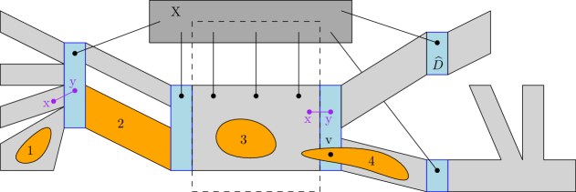
Figure 2: An illustration of the case analysis in Lemma 4.9. The graph $G-X$ has treewidth bounded by $\eta$ and $\widehat{D}\subseteq V(G)\setminus X$ is the union of vertices from the marked bags, drawn in blue. The light-gray polygons are the connected components of $G-(X\cup\widehat{D})$. Each orange set represents $C_{sim}$ in some scenario. The options 1 and 2 illustrate the Case (1.a.i). If $C_{sim}$ is a proper subset of $\widehat{C}$ (the gray one in option 1) then $(C_{sim},S)$ is not $\vartriangleleft$-maximal. If $C_{sim}=\widehat{C}$ then $S$ is located within two bags of the tree decomposition of $G-X$ and this option boils down to Lemma 4.8. The option 3 corresponds to Case (1.a.ii). Here the dashed rectangle depicts the interior of a $\vartriangleleft$-greater simple $\eta$-separation (denoted $(C^{v}_{sim},S_{v})$ in the proof) which covers the three vertices from $N(X)$ as well as $C_{sim}$. Also, two arrangements of the edge $xy$ from Case (2.a) are showed in purple. The option 4 illustrates Case (1.b) with $v\in C_{sim}\cap\widehat{D}$. By Lemma 4.4 the set $S=N(C_{sim})$ must be an important $(v,X)$-separator.

1. We bound the number of semi-simple $\eta$-separations in ${\mathcal{S}}(G,\eta)_{X}^{-}$. Let $\mathcal{B}_{X}^{-}$ be the family of subsets $S\subseteq V(G)\setminus X$ for which there exists $C_{sim}\subseteq V(G)\setminus X$ such that $(C_{sim},S)$ is a $\vartriangleleft$-maximal simple $\eta$-separation in $G$. By 4.6(3) for each semi-simple $(C,S)\in{\mathcal{S}}(G,\eta)_{X}^{-}$ there exists $C_{sim}\subseteq C$ so that $(C_{sim},S)$ is a $\vartriangleleft$-maximal simple $\eta$-separation. Hence by 4.6(5) the number of semi-simple $\eta$-separations in ${\mathcal{S}}(G,\eta)_{X}^{-}$ is bounded by $|\mathcal{B}_{X}^{-}|$ and it suffices to estimate the latter quantity.

   Let $S\in\mathcal{B}_{X}^{-}$ and $C_{sim}\subseteq V(G)\setminus X$ be such that $(C_{sim},S)$ is a $\vartriangleleft$-maximal simple $\eta$-separation.

   1. Suppose that $C_{sim}\cap\widehat{D}=\emptyset$. Let $\widehat{C}$ induce the connected component of $G-(X\cup\widehat{D})$ that contains $C_{sim}$.

      1. Suppose that $\widehat{C}\cap N_{G}(X)=\emptyset$. By Lemma 3.5 the set $N_{G-X}(\widehat{C})=N_{G}(\widehat{C})$ is contained in at most two bags from $L$ so $|N_{G}(\widehat{C})|\leq 2\eta+2$ and $(\widehat{C},N_{G}(\widehat{C}))$ forms a simple $\eta$-separation. If $C_{sim}$ was a proper subset of $\widehat{C}$ then it would not be $\vartriangleleft$-maximal. Hence $C_{sim}$ corresponds to a connected component of $(G-X)-\widehat{D}$: we have $C_{sim}=\widehat{C}$ and $S=N_{G}(\widehat{C})$. Lemma 4.8 bounds the number of distinct neighborhoods of such components: the number of possibilities for the choice of such $S$ is bounded by $2^{\mathcal{O}(\eta)}\cdot|L|+1\leq 2^{\mathcal{O}(\eta)}\cdot|{\mathcal{S}}_{X}|$. Here we exploited the fact that $|L|\leq 4(\eta+1)\cdot|{\mathcal{S}}_{X}|$ and that $|{\mathcal{S}}_{X}|\geq 1$.

      2. Now consider the case $\widehat{C}\cap N_{G}(X)\neq\emptyset$. Let $v\in\widehat{C}\cap N_{G}(X)$ and $u$ be its neighbor in $X$ that has been used during the construction of ${\mathcal{S}}_{X}$. Then there exists $(C_{v},S_{v})\in{\mathcal{S}}_{X}$ for which $\{u,v\}\subseteq C_{v}\cup S_{v}$. If $(C_{v},S_{v})$ was an edge-pair we would have marked the vertex $v$ but since $v\not\in\widehat{D}$ then $(C_{v},S_{v})$ must be semi-simple. We also know that $v\in C_{v}$ because $v$ is not marked.

         Let $C^{v}_{sim}=R_{G-S_{v}}(v)$; then $(C^{v}_{sim},S_{v})$ is a simple $\eta$-separation because $(C_{v},S_{v})$ is semi-simple. We have $\widehat{C}\cap S_{v}=\emptyset$ (because $S_{v}\setminus X\subseteq\widehat{D}$ by the marking scheme) so $C^{v}_{sim}\supseteq\widehat{C}\supseteq C_{sim}$. See Figure 2 for a visualization. In addition, $N_{G}[C^{v}_{sim}]\cap X\neq\emptyset$ implies that $C^{v}_{sim}\neq C_{sim}$ and so $(C_{sim},S)$ is not $\vartriangleleft$-maximal; a contradiction.

   2. Suppose that $C_{sim}\cap\widehat{D}\neq\emptyset$. Let $v\in C_{sim}\cap\widehat{D}$. From Lemma 4.4 we know that $S$ must be an important $(v,X)$-separator. For each $v\in\widehat{D}$ the number of important $(v,X)$-separators of size $\leq(2\eta+2)$ is bounded by $4^{2\eta+2}=2^{\mathcal{O}(\eta)}$ (Lemma 3.1). Therefore the maximal number of sets $S$ occurring in this scenario is $2^{\mathcal{O}(\eta)}\cdot|\widehat{D}|\leq 2^{\mathcal{O}(\eta)}\cdot|{\mathcal{S}}_{X}|$.

2. We bound the number of edge-pairs in ${\mathcal{S}}(G,\eta)_{X}^{-}$. When $(C,S)\in{\mathcal{S}}(G,\eta)_{X}^{-}$ is an edge-pair then $S=\{x,y\}$ for some $xy\in E(G-X)$ and $C=\emptyset$. By 4.6(2) we know that there can be no simple $\eta$-separation $(C^{\prime},S^{\prime})$ in $G$ for which $\{x,y\}\subseteq C^{\prime}\cup S^{\prime}$.

   1. Suppose that $\{x,y\}\not\subseteq\widehat{D}$. W.l.o.g. assume that $x\not\in\widehat{D}$. Let $\widehat{C}$ induce the connected component of $G-(X\cup\widehat{D})$ that contains $x$.

      1. If $\widehat{C}\cap N_{G}(X)=\emptyset$, we can use an analogous argument as in Case (1.a.i): $\{x,y\}\subseteq N[\widehat{C}]$ so $(\widehat{C},N_{G}(\widehat{C}))$ is a simple $\eta$-separation covering $xy$; a contradiction.

      2. If $\widehat{C}\cap N_{G}(X)\neq\emptyset$, we follow the argument from Case (1.a.ii): we use an arbitrary $v\in\widehat{C}\cap N_{G}(X)$ to certify the existence of a simple $\eta$-separation $(C^{v}_{sim},S_{v})$ for which $\widehat{C}\subseteq C^{v}_{sim}$. Then again $\{x,y\}\subseteq N_{G}[\widehat{C}]\subseteq N_{G}[C^{v}_{sim}]$ yields a contradiction.

   2. In remains to handle the case $\{x,y\}\subseteq\widehat{D}$. Then $xy$ is an edge in the graph $G[\widehat{D}]$. But the treewidth of this graph is at most $\eta$ so the number of edges in $G[\widehat{D}]$ is bounded by $\eta\cdot|\widehat{D}|\leq 4(\eta+1)^{3}\cdot|{\mathcal{S}}_{X}|$ (Lemma 3.2).

We have established that $|{\mathcal{S}}(G,\eta)_{X}^{-}|\leq 2^{\mathcal{O}(\eta)}\cdot|{\mathcal{S}}_{X}|$. Recall that ${\mathcal{S}}_{X}\subseteq{\mathcal{S}}(G,\eta)_{X}^{+}$. This implies that $|{\mathcal{S}}(G,\eta)|=|{\mathcal{S}}(G,\eta)_{X}^{+}|+|{\mathcal{S}}(G,\eta)_{X}^{-}|\leq|{\mathcal{S}}(G,\eta)_{X}^{+}|+2^{\mathcal{O}(\eta)}\cdot|{\mathcal{S}}_{X}|\leq 2^{\mathcal{O}(\eta)}\cdot|{\mathcal{S}}(G,\eta)_{X}^{+}|$, as promised. ∎

To derive Theorem 1.1 from Lemma 4.9, recall that when $(C,S)$ is an $\eta$-separation then $(C\cup S)$ is a $(3\eta+2)$-protrusion. Hence ${\mathcal{S}}(G,\eta)$ constitutes an $(\eta,3\eta+2,2^{\mathcal{O}(\eta)})$-modulator hitting family. The size bound and the running time to construct ${\mathcal{S}}(G,\eta)$ follow from Lemma 4.7.

5 Exhaustive families

We explain how to enumerate the relevant partial solutions within an $r$-protrusion with Courcelle’s Theorem. A similar idea has been used for trimming the space of partial solutions in DP algorithms on tree decomposition [8, 30]. Our treatment of protrusions is a combination of ideas from [48] for processing protrusion decompositions and from [40] for processing hybrid graph decompositions. We adapt their methods to the weighted setting.

Definition 5.1 ([40]).

Let $\mathcal{F}$ be a finite family of graphs and $A$ be a vertex subset in a node-weighted graph $G$. We say that a family $\mathcal{A}\subseteq 2^{A}$ of subsets of $A$ is $(A,\mathcal{F})$-exhaustive if for every $\mathcal{F}$-minor hitting set $X$ there exists $X_{A}\in\mathcal{A}$ such that $X^{\prime}=(X\setminus A)\cup X_{A}$ is also an $\mathcal{F}$-minor hitting set and $w(X^{\prime})\leq w(X)$.

Additionally, for $\ell\in\mathbb{N}$ we say that a family $\mathcal{A}\subseteq 2^{A}$ of size-$(\leq\ell)$ subsets of $A$ is $(A,\mathcal{F},\ell)$-exhaustive if for every $\mathcal{F}$-minor hitting set $X$ satisfying $|X\cap A|\leq\ell$ there exists $X_{A}\in\mathcal{A}$ such that $X^{\prime}=(X\setminus A)\cup X_{A}$ is also an $\mathcal{F}$-minor hitting set and $w(X^{\prime})\leq w(X)$.

When $X$ is an optimal solution then the replacement $X_{A}$ cannot be cheaper than $X\cap A$ as otherwise we would have $w(X^{\prime})<w(X)$. In particular, whenever $X$ is optimal and $X\cap A$ is non-empty then $w(X_{A})=w(X\cap A)>0$ so $X_{A}$ must be non-empty as well.

Observation 5.2.

Let $X$ be an optimal $\mathcal{F}$-minor hitting set in $G$, $A$ be a vertex subset intersecting $X$, and $\mathcal{A}\subseteq 2^{A}$ be an $(A,\mathcal{F})$-exhaustive family. Then there exists a non-empty $X_{A}\in\mathcal{A}$ such that $\mathsf{opt}_{\mathcal{F}}(G)-\mathsf{opt}_{\mathcal{F}}(G-X_{A})=w(X_{A})$.

An analogous statement holds for $k$-optimal solutions as well but the justification is slightly less obvious so we provide a full proof.

Lemma 5.3.

Let $k,\ell\geq 1$, $X$ be a $k$-optimal $\mathcal{F}$-minor hitting set in $G$, $A$ be a vertex subset satisfying $|X\cap A|=\ell$, and $\mathcal{A}\subseteq 2^{A}$ be an $(A,\mathcal{F},\ell)$-exhaustive family. Then there exists a non-empty $X_{A}\in\mathcal{A}$ such that $\mathsf{opt}_{\mathcal{F},k}(G)-\mathsf{opt}_{\mathcal{F},k-\ell}(G-X_{A})=w(X_{A})$.

Proof.

By the definition of an $(A,\mathcal{F},\ell)$-exhaustive family there exists $X_{A}\in\mathcal{A}$ such that $|X_{A}|\leq\ell$, $X^{\prime}=(X\setminus A)\cup X_{A}$ is an $\mathcal{F}$-minor hitting set, and $w(X^{\prime})\leq w(X)$. We have $|X^{\prime}|=|X\setminus A|+|X_{A}|\leq(k-\ell)+\ell=k$. But $X$ is $k$-optimal so in fact we must have $w(X^{\prime})=w(X)$ and $w(X_{A})=w(X\cap A)$. In particular, this implies that $X_{A}\neq\emptyset$ because $w(X\cap A)>0$ by assumption. Next, $X\setminus A$ forms an $\mathcal{F}$-minor hitting set in $G-X_{A}$ of size $\leq k-\ell$ so $\mathsf{opt}_{\mathcal{F},k-\ell}(G-X_{A})\leq w(X\setminus A)=w(X)-w(X\cap A)=\mathsf{opt}_{\mathcal{F},k}(G)-w(X_{A})$. On the other hand, we have $\mathsf{opt}_{\mathcal{F},k}(G)\leq\mathsf{opt}_{\mathcal{F},k-\ell}(G-X_{A})+w(X_{A})$ so in fact these two quantities must be equal. ∎

We take advantage of the fact that when $A$ is an $r$-protrusion then the graph $G-A$ can “communicate” with $A$ only through $\partial(A)$. To construct the exhaustive families, we utilize the bounds on the minimum-sized representatives in the the relation $\equiv_{h}$ over boundaried graphs [9]. The following proof is similar in spirit to [41, Lemma 5.33]. The difference is that here we compute partial solutions using an FPT algorithm parameterized by treewidth while therein they were computed with an FPT algorithm parameterized by the solution size.

Lemma 5.4.

There is a computable function $f\colon\mathbb{N}^{2}\to\mathbb{N}$ so that the following holds. Let $r,h\in\mathbb{N}$ and $\mathcal{F}$ be a family of graphs with sizes bounded by $h$. Next, let $A\subseteq V(G)$ be an $r$-protrusion in a graph $G$. Then there exists an $(A,\mathcal{F})$-exhaustive family $\mathcal{A}\subseteq 2^{A}$ of size at most $f(h,r)$ and it can be computed in time $f(h,r)\cdot|V(G)|^{\mathcal{O}(1)}$.

Furthermore, for each $\ell\in\mathbb{N}$ there exists an $(A,\mathcal{F},\ell)$-exhaustive family $\mathcal{A}\subseteq 2^{A}$ of size at most $f(h,r)$ and it can be computed in time $f(h,r)\cdot|V(G)|^{\mathcal{O}(1)}$.

Proof.

Recall that $\partial_{G}(A)=N_{G}(V(G)\setminus A)$. We will also denote $A\setminus\partial_{G}(A)$ by $\triangle_{G}(A)$. We first give an algorithm to construct a family $\mathcal{A}\subseteq 2^{A}$ and then we will prove that it is $(A,\mathcal{F})$-exhaustive.

We begin by computing families $\mathcal{R}_{h}^{(\ell)}$ for each $\ell\in[r]$ (Corollary 3.10). For each subset $S\subseteq\partial_{G}(A)$ consider the graph $G-S$, in which $A\setminus S$ still forms an $r$-protrusion. Let $\ell=|\partial_{G}(A)\setminus S|$ and consider the boundaried graph $\mathbf{G}_{S}=(G[A\setminus S],\partial_{G-S}(A\setminus S),\rho)$ where $\rho$ is an arbitrary labeling. Next, for each $\mathbf{H}\in\mathcal{R}_{h}^{(\ell)}$ that is compatible with $\mathbf{G}_{S}$, consider the graph $G_{S,H}=\mathbf{G}_{S}\oplus\mathbf{H}$. We define the weight function on $G_{S,H}$ by preserving the weights from $G$ on $\triangle_{G}(A)$ and setting the remaining weights to $\infty$. Note that the size of $\mathbf{H}$ is bounded by some function of $h$ and $r$ (Corollary 3.10) so the treewidth of $G_{S,H}$ is likewise bounded. Therefore, we can take advantage of Theorem 3.11 to solve Weighted $\mathcal{F}$-M-Deletion on $G_{S,H}$ in time $f(h,r)\cdot|V(G_{S,H})|^{\mathcal{O}(1)}$; let $X_{H}$ denote the computed optimal solution. If there is no finite-weight solution then we move on to the next $\mathbf{H}\in\mathcal{R}_{h}^{(\ell)}$, otherwise we have $X_{H}\subseteq\triangle_{G}(A)$. In this case we insert $S\cup X_{H}$ into $\mathcal{A}$. The size of $\mathcal{A}$ can be bounded by the number of choices of $S$, that is, $2^{r}$, times the bound on $|\mathcal{R}_{h}^{(\ell)}|$, for $\ell\leq r$, which follows from Corollary 3.10.

We argue that $\mathcal{A}$ is $(A,\mathcal{F})$-exhaustive. Consider an $\mathcal{F}$-minor hitting set $X$. Let $\widehat{S}=X\cap\partial_{G}(A)$ and $\mathbf{G}^{X}=(G-(X\cup\triangle_{G}(A)),\partial_{G}(A)\setminus X,\rho)$; note that $\mathbf{G}^{X}\oplus\mathbf{G}_{\widehat{S}}=G-(X\setminus\triangle_{G}(A))$. Next, let $\mathbf{H}\in\mathcal{R}_{h}^{(\ell)}$ be a boundaried graph that is $\equiv_{h}$-equivalent to $\mathbf{G}^{X}$. By 3.8 set $Y\subseteq\triangle_{G}(A)$ is an $\mathcal{F}$-minor hitting set in $\mathbf{G}^{X}\oplus\mathbf{G}_{\widehat{S}}$ if and only if it is an $\mathcal{F}$-minor hitting set in $\mathbf{H}\oplus\mathbf{G}_{\widehat{S}}$. Consequently, $X\cap\triangle_{G}(A)$ is an $\mathcal{F}$-minor hitting set in $\mathbf{H}\oplus\mathbf{G}_{\widehat{S}}$. This means that the algorithm above must have detected some $X_{H}\subseteq\triangle_{G}(A)$ of weight $w(X_{H})\leq w(X\cap\triangle_{G}(A))$ and inserted $\widehat{S}\cup X_{H}$ into $\mathcal{A}$. On the other hand, $X_{H}$ forms an $\mathcal{F}$-minor hitting set in $\mathbf{G}^{X}\oplus\mathbf{G}_{\widehat{S}}=G-(X\setminus\triangle_{G}(A))$. So $X^{\prime}=(X\setminus\triangle_{G}(A))\cup X_{H}$ is an $\mathcal{F}$-minor hitting set in $G$ and $w(X^{\prime})\leq w(X)$. As $X\cap\partial_{G}(A)=\widehat{S}$ we can alternatively write $X^{\prime}=(X\setminus A)\cup(\widehat{S}\cup X_{H})$. This means that $\mathcal{A}$ includes a replacement for $X\cap A$ and proves that $\mathcal{A}$ is indeed $(A,\mathcal{F})$-exhaustive.

Constructing an $(A,\mathcal{F},\ell)$-exhaustive family is analogous. The only difference is that when considering the graph $G_{S,H}$ we compute an $\ell$-optimal solution, i.e., a minimum-weight $\mathcal{F}$-minor hitting set among those on at most $\ell$ vertices. This is doable within the same time bound (Theorem 3.11).∎

6 Applications

6.1 The approximation algorithm

For the ease of presentation, we first give an algorithm for Weighted Treewidth-$\eta$ Deletion and then use it as a subroutine to solve general Weighted Planar $\mathcal{F}$-M-Deletion. We begin with the analysis of a single iteration and compare the expected drop in the optimum to the expected cost of the sampled partial solution.

Lemma 6.1.

For each $\eta\in\mathbb{N}$ there is a constant $c\in\mathbb{N}$ and an algorithm that, given a node-weighted $n$-vertex graph $G$ with $\mathrm{\textbf{tw}}(G)>\eta$, runs in time $\mathcal{O}_{\eta}\left(n^{\mathcal{O}(\eta)}\right)$, and outputs a non-empty random subset $Y\subseteq V(G)$ with a following guarantee.

$$\mathbb{E}\left[w(Y)\right]\leq c\cdot\mathbb{E}\left[\mathsf{opt}_{\eta}(G)-\mathsf{opt}_{\eta}(G-Y)\right]$$

Proof.

We apply Theorem 1.1 to compute an $(\eta,r,c_{1})$-modulator hitting family $\mathcal{P}$ for $G$ with $r=\mathcal{O}(\eta)$ and $c_{1}=2^{\mathcal{O}(\eta)}$. This takes time $n^{\mathcal{O}(\eta)}$. Next, we use Lemma 5.4 to compute, for each $A\in\mathcal{P}$, an $(A,\mathcal{F}(\eta))$-exhaustive family $\mathcal{A}_{A}$ of size $\leq c_{2}$, where $c_{2}=f(\max_{F\in\mathcal{F}(\eta)}|V(F)|,r)$ and $f$ is the function from that lemma. This takes time $n^{\mathcal{O}(\eta)}\cdot\mathcal{O}_{\eta}\left(n^{\mathcal{O}(1)}\right)$. Note that $c_{1},c_{2}$ are constants depending only on $\eta$ and recall that a graph has treewidth bounded by $\eta$ if and only if it is $\mathcal{F}(\eta)$-minor-free so $\mathsf{opt}_{\eta}(G)=\mathsf{opt}_{\mathcal{F}(\eta)}(G)$. Now, consider the family $\mathcal{B}$ of all pairs $(A,Y)$ where $A\in\mathcal{P}$ and $Y\in\mathcal{A}_{A}$ is non-empty. We sample an element $(A,Y)$ from $\mathcal{B}$ with probability proportional to $\frac{1}{w(Y)}$. Note that $w(Y)>0$ because $Y\neq\emptyset$. Let $\widehat{Y}$ denote the corresponding random variable.

We claim that the random variable $\widehat{Y}$ satisfies the guarantee of the lemma. Let $W=\sum_{(A,Y)\in\mathcal{B}}\frac{1}{w(Y)}$. Then the probability of choosing a pair $(A,Y)$ equals $\frac{1}{w(Y)\cdot W}$. We have

$$\mathbb{E}\left[w(\widehat{Y})\right]=\sum_{(A,Y)\in\mathcal{B}}w(Y)\cdot\frac{1}{w(Y)\cdot W}=\frac{|\mathcal{B}|}{W}.$$

Now we estimate the expected value of $\mathsf{opt}_{\eta}(G)-\mathsf{opt}_{\eta}(G-\widehat{Y})$. Clearly, for every $Y$ this quantity is non-negative. Let $X$ be an optimal solution to Weighted Treewidth-$\eta$ Deletion on $G$. By the definition of a modulator hitting family, we know that there is a subfamily $\mathcal{P}_{X}\subseteq\mathcal{P}$ of size at least $|\mathcal{P}|/c_{1}$ so that for each $A\in\mathcal{P}_{X}$ we have $A\cap X\neq\emptyset$. Furthermore, 5.2 implies that for each $A\in\mathcal{P}_{X}$ there is some non-empty $Y_{A}\in\mathcal{A}_{A}$ satisfying $\mathsf{opt}_{\eta}(G)-\mathsf{opt}_{\eta}(G-Y_{A})=w(Y_{A})$. In particular, we have $(A,Y_{A})\in\mathcal{B}$ and we can estimate

$$\mathbb{E}\left[\mathsf{opt}_{\eta}(G)-\mathsf{opt}_{\eta}(G-\widehat{Y})\right]\geq\sum_{A\in\mathcal{P}_{X}}w(Y_{A})\cdot\frac{1}{w(Y_{A})\cdot W}=\frac{|\mathcal{P}_{X}|}{W}.$$

It holds that $|\mathcal{B}|\leq c_{2}\cdot|\mathcal{P}|\leq c_{2}\cdot c_{1}\cdot|\mathcal{P}_{X}|$. Hence the claimed inequality holds for $c=c_{1}\cdot c_{2}$. ∎

In the proof it was important that when $Y\subseteq V(G)$ belongs to multiple $(A_{i},\mathcal{F}(\eta))$-exhaustive families for different sets $(A_{i})$ then we consider all its copies in the family $\mathcal{B}$. Alternatively, we could multiply the probability of choosing $Y$ by the number of such sets $(A_{i})$. By the same reason we had to include the factor $\deg(v)$ in the probabilities in the simplified algorithm for Weighted Feedback Vertex Set in Section 2.

We will perform the described sampling iteratively. At each step, the expected value of the revealed part of a solution is within a factor $c$ from the cost of the chosen set $Y$. The algorithm is terminated when the value of optimum drops to 0, so the expected value of $w(Y_{1})+w(Y_{2})+\dots$ should be bounded by $c$ times the initial optimum. We will formalize this intuition by analyzing a random process being a supermartingale (see Section 3).

Lemma 6.2.

For each $\eta\in\mathbb{N}$ there is a constant $c\in\mathbb{N}$ and a randomized algorithm that, given a node-weighted $n$-vertex graph $G$ graph $G$, runs in time $\mathcal{O}_{\eta}\left(n^{\mathcal{O}(\eta)}\right)$, and outputs a treewidth-$\eta$ modulator $X$ in $G$ such that $\mathbb{E}\left[w(X)\right]\leq c\cdot\mathsf{opt}_{\eta}(G)$.

Proof.

We will use the constant $c$ defined in Lemma 6.1. Consider the following random process $(X_{i})$ where $X_{i}\subseteq V(G)$. We start with $X_{0}=\emptyset$. Next, for $i\geq 0$ we compute a random non-empty subset $Y_{i+1}\subseteq V(G)\setminus X_{i}$ by applying Lemma 6.1 to the graph $G_{i}=G-X_{i}$. Then we set $X_{i+1}=X_{i}\cup Y_{i+1}$. The process stops at iteration $\tau$ when $\mathrm{\textbf{tw}}(G_{\tau})$ becomes bounded by $\eta$ and the algorithm returns $X=X_{\tau}$. Note that $X_{i}$ grows at each iteration so $\tau$ is always bounded by $|V(G)|$. We will show that $X$ is a $c$-approximate solution in expectation.

We claim that the process $P_{i}=w(X_{i})+c\cdot\mathsf{opt}_{\eta}(G_{i})$ is a supermartingale, which means that $\mathbb{E}\left[P_{i+1}\mid P_{0},\dots P_{i}\right]\leq P_{i}$. This condition is equivalent to $\mathbb{E}\left[P_{i+1}-P_{i}\mid P_{0},\dots P_{i}\right]\leq 0$.

$$P_{i+1}-P_{i}=w(Y_{i+1})+c\cdot\left(\mathsf{opt}_{\eta}(G_{i+1})-\mathsf{opt}_{\eta}(G_{i})\right)=w(Y_{i+1})-c\cdot\left(\mathsf{opt}_{\eta}(G_{i})-\mathsf{opt}_{\eta}(G_{i}-Y_{i+1})\right)$$

Lemma 6.1 states that the expected value of such a random variable is upper bounded by 0 for any fixed graph $G_{i}$. Hence the process $(P_{i})$ is indeed a supermartingale. Consider the stopping time $\tau$, for which it holds that $\mathsf{opt}_{\eta}(G_{\tau})=0$. We can now take advantage of the Doob’s Optional-Stopping Theorem (3.13) which states that $\mathbb{E}\left[P_{\tau}\right]\leq\mathbb{E}\left[P_{0}\right]$.

$$\mathbb{E}\left[w(X)\right]=\mathbb{E}\left[w(X_{\tau})+c\cdot\mathsf{opt}_{\eta}(G_{\tau})\right]=\mathbb{E}\left[P_{\tau}\right]\leq\mathbb{E}\left[P_{0}\right]=w(X_{0})+c\cdot\mathsf{opt}_{\eta}(G_{0})=c\cdot\mathsf{opt}_{\eta}(G)$$

This concludes the proof. ∎

Finally, we solve Weighted Planar $\mathcal{F}$-M-Deletion by first reducing the treewidth to $\eta(\mathcal{F})$.

See 1.2

Proof.

Any $\mathcal{F}$-minor hitting set is also a treewidth-$\eta(\mathcal{F})$ modulator so it holds that $\mathsf{opt}_{\eta(\mathcal{F})}(G)\leq\mathsf{opt}_{\mathcal{F}}(G)$. We apply Lemma 6.2 to compute a set $X_{1}\subseteq V(G)$ such that $\mathrm{\textbf{tw}}(G-X_{1})\leq\eta(\mathcal{F})$ and $\mathbb{E}\left[w(X_{1})\right]\leq c\cdot\mathsf{opt}_{\eta(\mathcal{F})}(G)$. Since the treewidth of $G-X_{1}$ is bounded, we can now solve Weighted $\mathcal{F}$-M-Deletion optimally on $G-X_{1}$ using Theorem 3.11. We compute $X_{2}\subseteq V(G)\setminus X_{1}$ such that $w(X_{2})=\mathsf{opt}_{\mathcal{F}}(G-X_{1})\leq\mathsf{opt}_{\mathcal{F}}(G)$. The union $X_{1}\cup X_{2}$ forms a solution that is $(c+1)$-approximate in expectation. ∎

6.2 The single-exponential FPT algorithm

Unlike for approximation, this time we cannot afford to first solve Weighted Treewidth-$\eta$ Deletion and then process a bounded-treewidth graph, so we will treat the bounded-treewidth scenario as a special case in the branching algorithm. The main difference compared to Theorem 1.2 is that now we will sample both the protrusion $A\in\mathcal{P}$ and the replacement $Y\in\mathcal{A}$ according to a uniform distribution. We also need to guess the integer $\ell=|X\cap A|$ to guide the construction of an $(A,\mathcal{F},\ell)$-exhaustive family; note that we can compute such a family of size $\mathcal{O}_{\mathcal{F}}(1)$ only when $\ell$ is known. However, we cannot sample $\ell$ uniformly from $[1,k]$ because when the correct value of $\ell$ is always $\mathcal{O}(1)$ we need to achieve constant success probability in every step. As a remedy, we will use geometric distribution to sample $\ell$.

See 1.3

Proof.

We will abbreviate $\eta=\eta(\mathcal{F})$. Consider an instance $(G,k)$ and proceed as follows. If $k=0$ check if $G$ is $\mathcal{F}$-minor-free in time $\mathcal{O}_{\mathcal{F}}(n)$ (Theorem 3.6); if yes return an empty set and otherwise abort the computation. If $\mathrm{\textbf{tw}}(G)\leq\eta$ solve the problem optimally in time $\mathcal{O}_{\mathcal{F}}(n^{\mathcal{O}(1)})$ using Theorem 3.11.

We will assume now that $k\geq 1$ and $\mathrm{\textbf{tw}}(G)>\eta$. In order to prepare a recursive call, we make three random choices.

1. Use Theorem 1.1 to compute an $(\eta,r,c_{1})$-modulator hitting family $\mathcal{P}$ for $r=\mathcal{O}(\eta)$ and $c_{1}=2^{\mathcal{O}(\eta)}$. This takes time $n^{\mathcal{O}(\eta)}$. Then choose a set $A\in\mathcal{P}$ uniformly at random.

2. Consider a random variable $L\in[1,k]$ where the probability of choosing $L=\ell$ is proportional to $2^{-\ell}$. Note that we have $\mathbb{P}\left[L=\ell\right]\geq 2^{-\ell}$ for each $\ell\in[1,k]$.

3. Use Lemma 5.4 to compute an $(A,\mathcal{F},L)$-exhaustive family $\mathcal{A}$ of size $\leq c_{2}$, where $c_{2}=f(\max_{F\in\mathcal{F}}|V(F)|,r)$ and $f$ is the function from that lemma. This takes time $\mathcal{O}_{\mathcal{F}}(n^{\mathcal{O}(1)})$. Then choose a non-empty set $Y\in\mathcal{A}$ again uniformly at random (if $\mathcal{A}=\{\emptyset\}$ abort the computation). Add $Y$ to the solution and recurse on $(G-Y,k-L)$.

Let $Q(G,k)$ denote the event that the algorithm returns a $k$-optimal solution to the instance $(G,k)$ under an assumption that $\mathsf{opt}_{\mathcal{F},k}(G)<\infty$. We will prove that $\mathbb{P}\left[Q(G,k)\right]\geq(2c_{1}c_{2})^{-k}$ by induction on $k$. The claim clearly holds for $k=0$ so we will assume that $k>0$ and that the claim holds for all $k^{\prime}<k$. First, if $\mathrm{\textbf{tw}}(G)\leq\eta$ then the algorithm always returns a $k$-optimal solution. We will now assume $\mathrm{\textbf{tw}}(G)>\eta$ and analyze the three random guesses performed before a recursive call.

Let $X$ be a fixed $k$-optimal solution to Weighted $\mathcal{F}$-M-Deletion. It is also a solution to Weighted Treewidth-$\eta$ Deletion. By Definition 3.3 of an $(\eta,r,c_{1})$-modulator hitting family, we know that $\mathbb{P}\left[A\cap X\neq\emptyset\right]\geq 1/c_{1}$ for a random choice of $A\in\mathcal{P}$. Suppose that $A$ has been chosen successfully and let $\ell_{A}=|A\cap X|\geq 1$. Then $\mathbb{P}\left[L=\ell_{A}\right]\geq 2^{-\ell_{A}}$. Lemma 5.3 states that the $(A,\mathcal{F},\ell_{A})$-exhaustive family $\mathcal{A}$ contains a non-empty set $X_{A}$ of size $\leq\ell_{A}$ for which $\mathsf{opt}_{\mathcal{F},k}(G)-\mathsf{opt}_{\mathcal{F},k-\ell_{A}}(G-X_{A})=w(X_{A})$. The probability of choosing $Y=X_{A}$ in the third step is $1/|\mathcal{A}|\geq 1/c_{2}$. The call $(G,k)$ will be processed correctly if all these guesses are correct and the call $(G-X_{A},k-\ell_{A})$ is processed correctly. We are ready to estimate the probability of $Q(G,k)$, by first analyzing the success probability for a fixed $A\in\mathcal{P}$.

$$\mathbb{P}\left[Q(G,k)\mid A\cap X\neq\emptyset\right] \geq\mathbb{P}\left[L=\ell_{A}\right]\cdot\mathbb{P}\left[Y=X_{A}\right]\cdot\mathbb{P}\left[Q(G-X_{A},k-\ell_{A})\right]$$

$$\geq 2^{-\ell_{A}}\cdot c_{2}^{-1}\cdot(2c_{1}c_{2})^{-(k-\ell_{A})}\geq(2c_{2})^{-1}\cdot(2c_{1}c_{2})^{-(k-1)}$$

We have used the inductive assumption and the fact that $\ell_{A}\geq 1$ when $A\cap X\neq\emptyset$.

$$\mathbb{P}\left[Q(G,k)\right]\geq\mathbb{P}\left[A\cap X\neq\emptyset\right]\cdot\mathbb{P}\left[Q(G,k)\mid A\cap X\neq\emptyset\right]\geq c_{1}^{-1}\cdot(2c_{2})^{-1}\cdot(2c_{1}c_{2})^{-(k-1)}=(2c_{1}c_{2})^{-k}$$

We have thus proven that the success probability of the presented procedure is at least $c^{-k}$ for $c=2c_{1}c_{2}$ whereas its running time is $\mathcal{O}_{\mathcal{F}}\left(n^{\mathcal{O}(\eta)}\right)$. Note that if the computation has not been aborted, then the returned solution has at most $k$ vertices. We repeat this procedure $c^{k}$ many times and output the outcome with the smallest weight. This gives constant probability of witnessing a $k$-optimal solution. The total running time is $c^{k}\cdot\mathcal{O}_{\mathcal{F}}\left(n^{\mathcal{O}(\eta)}\right)=2^{\mathcal{O}_{\mathcal{F}}(k)}\cdot n^{\mathcal{O}(\eta)}$. ∎

7 Conclusion

We have shown that constant approximation for Planar $\mathcal{F}$-M-Deletion can be extended to the weighted setting, by introducing a new technique that circumvents the need to perform weighted protrusion replacement. There are several natural questions about potential refinements of Theorem 1.2. Can the algorithm be derandomized? Can we improve the running time so that the degree of the polynomial is a universal constant that does not depend on $\eta$? Can the approximation factor be bounded by a slowly growing function of $\eta$? All these improvements are possible in the unweighted realm [29, 37]. It is however unknown whether there exists a universal constant $c$ for which every unweighted Planar $\mathcal{F}$-M-Deletion problem admits a $c$-approximation algorithm.

Even though our approximation factor is a computable function of the treewidth bound, this function grows very rapidly. Is it possible to get a “reasonable” approximation factor (say, under 100) for Weighted Treewidth-2 Deletion or Weighted Outerplanar Deletion? In the unweighted setting, the approximation factor (for both problems) can be pinned down to 40 [23, 37]. As another potential direction, can we combine the ideas from Theorem 1.1 and the scaling lemma from [33] to improve the status of Weighted Planar $\mathcal{F}$-M-Deletion on $H$-minor-free graphs from QPTAS to PTAS?

One message of our work is that Planar $\mathcal{F}$-M-Deletion does not get any harder for approximation or FPT algorithms when we consider weighted graphs. What about a polynomial kernelization under parameterization by the number of vertices in the sought solution? While this is well-understood on unweighted graphs [29], we are only aware of a polynomial kernelization for Weighted Vertex Cover [24]. This result could be possibly extended to the weighted variants of Feedback Vertex Set, Treewidth-2 Deletion, and Outerplanar Deletion, for which we know kernelization algorithms based on explicit reductions rules [23, 66]. Does general Weighted Planar $\mathcal{F}$-M-Deletion admit a polynomial kernelization for every fixed family $\mathcal{F}$?

References

- [1] Akanksha Agrawal, Sudeshna Kolay, Daniel Lokshtanov, and Saket Saurabh. A faster FPT algorithm and a smaller kernel for block graph vertex deletion. In LATIN 2016: Theoretical Informatics: 12th Latin American Symposium, Ensenada, Mexico, April 11-15, 2016, Proceedings 12, pages 1–13. Springer, 2016.
- [2] Akanksha Agrawal, Daniel Lokshtanov, Pranabendu Misra, Saket Saurabh, and Meirav Zehavi. Polylogarithmic approximation algorithms for Weighted--Deletion problems. In Eric Blais, Klaus Jansen, José D. P. Rolim, and David Steurer, editors, Approximation, Randomization, and Combinatorial Optimization. Algorithms and Techniques, APPROX/RANDOM 2018, August 20-22, 2018 - Princeton, NJ, USA, volume 116 of LIPIcs, pages 1:1–1:15. Schloss Dagstuhl - Leibniz-Zentrum für Informatik, 2018.
- [3] Jungho Ahn, Eduard Eiben, O-joung Kwon, and Sang-il Oum. A polynomial kernel for 3-leaf power deletion. Algorithmica, 85(10):3058–3087, 2023.
- [4] Jungho Ahn, Eun Jung Kim, and Euiwoong Lee. Towards constant-factor approximation for chordal/distance-hereditary vertex deletion. Algorithmica, 84(7):2106–2133, 2022.
- [5] Vineet Bafna, Piotr Berman, and Toshihiro Fujito. A 2-approximation algorithm for the undirected feedback vertex set problem. SIAM Journal on Discrete Mathematics, 12(3):289–297, 1999.
- [6] Nikhil Bansal, Daniel Reichman, and Seeun William Umboh. Lp-based robust algorithms for noisy minor-free and bounded treewidth graphs. In Philip N. Klein, editor, Proceedings of the Twenty-Eighth Annual ACM-SIAM Symposium on Discrete Algorithms, SODA 2017, Barcelona, Spain, Hotel Porta Fira, January 16-19, pages 1964–1979. SIAM, 2017.
- [7] Reuven Bar-Yehuda and Shimon Even. A linear-time approximation algorithm for the weighted vertex cover problem. Journal of Algorithms, 2(2):198–203, 1981.
- [8] Julien Baste, Ignasi Sau, and Dimitrios M. Thilikos. Hitting minors on bounded treewidth graphs. I. General upper bounds. SIAM J. Discret. Math., 34(3):1623–1648, 2020.
- [9] Julien Baste, Ignasi Sau, and Dimitrios M. Thilikos. Hitting minors on bounded treewidth graphs. IV. An optimal algorithm. SIAM J. Comput., 52(4):865–912, 2023.
- [10] Ann Becker and Dan Geiger. Approximation algorithms for the loop cutset problem. In Uncertainty in Artificial Intelligence, pages 60–68. Elsevier, 1994.
- [11] Hans L Bodlaender. A linear-time algorithm for finding tree-decompositions of small treewidth. SIAM J. Comput., 25(6):1305–1317, 1996.
- [12] Hans L Bodlaender, Fedor V Fomin, Daniel Lokshtanov, Eelko Penninkx, Saket Saurabh, and Dimitrios M Thilikos. (Meta) kernelization. Journal of the ACM (JACM), 63(5):1–69, 2016.
- [13] Yixin Cao. Linear recognition of almost interval graphs. In Proceedings of the Twenty-Seventh Annual ACM-SIAM Symposium on Discrete Algorithms, pages 1096–1115. SIAM, 2016.
- [14] Jianer Chen, Fedor V Fomin, Yang Liu, Songjian Lu, and Yngve Villanger. Improved algorithms for feedback vertex set problems. Journal of Computer and System Sciences, 74(7):1188–1198, 2008.
- [15] Jianer Chen, Iyad A Kanj, and Ge Xia. Improved upper bounds for vertex cover. Theoretical Computer Science, 411(40-42):3736–3756, 2010.
- [16] Fabián A Chudak, Michel X Goemans, Dorit S Hochbaum, and David P Williamson. A primal–dual interpretation of two 2-approximation algorithms for the feedback vertex set problem in undirected graphs. Operations Research Letters, 22(4-5):111–118, 1998.
- [17] Julia Chuzhoy and Zihan Tan. Towards tight (er) bounds for the excluded grid theorem. Journal of Combinatorial Theory, Series B, 146:219–265, 2021.
- [18] Marek Cygan, Fedor V. Fomin, Lukasz Kowalik, Daniel Lokshtanov, Dániel Marx, Marcin Pilipczuk, Michał Pilipczuk, and Saket Saurabh. Parameterized Algorithms. Springer, 2015.
- [19] Marek Cygan, Daniel Lokshtanov, Marcin Pilipczuk, Michał Pilipczuk, and Saket Saurabh. Minimum bisection is fixed parameter tractable. In Proceedings of the forty-sixth annual ACM symposium on Theory of computing, pages 323–332, 2014.
- [20] Marek Cygan, Marcin Pilipczuk, Michał Pilipczuk, and Jakub Onufry Wojtaszczyk. An improved FPT algorithm and a quadratic kernel for pathwidth one vertex deletion. Algorithmica, 64:170–188, 2012.
- [21] Erik D Demaine and Mohammad Taghi Hajiaghayi. Bidimensionality: new connections between FPT algorithms and PTASs. In SODA, volume 5, pages 590–601, 2005.
- [22] R. Diestel. Graph theory 3rd ed. Graduate texts in mathematics, 173(33):12, 2005.
- [23] Huib Donkers, Bart M. P. Jansen, and Michał Włodarczyk. Preprocessing for outerplanar vertex deletion: An elementary kernel of quartic size. Algorithmica, 84(11):3407–3458, 2022.
- [24] Michael Etscheid, Stefan Kratsch, Matthias Mnich, and Heiko Röglin. Polynomial kernels for weighted problems. J. Comput. Syst. Sci., 84:1–10, 2017.
- [25] Michael R Fellows and Michael A Langston. Nonconstructive tools for proving polynomial-time decidability. Journal of the ACM (JACM), 35(3):727–739, 1988.
- [26] Michael R Fellows and Michael A Langston. An analogue of the Myhill-Nerode theorem and its use in computing finite-basis characterizations. In 30th Annual Symposium on Foundations of Computer Science, pages 520–525. IEEE Computer Society, 1989.
- [27] Samuel Fiorini, Gwenaël Joret, and Ugo Pietropaoli. Hitting diamonds and growing cacti. In International Conference on Integer Programming and Combinatorial Optimization, pages 191–204. Springer, 2010.
- [28] Fedor V. Fomin, Daniel Lokshtanov, Dániel Marx, Marcin Pilipczuk, Michał Pilipczuk, and Saket Saurabh. Subexponential parameterized algorithms for planar and apex-minor-free graphs via low treewidth pattern covering. SIAM J. Comput., 51(6):1866–1930, 2022.
- [29] Fedor V. Fomin, Daniel Lokshtanov, Neeldhara Misra, and Saket Saurabh. Planar -Deletion: Approximation, kernelization and optimal FPT algorithms. In 53rd Annual IEEE Symposium on Foundations of Computer Science, FOCS 2012, New Brunswick, NJ, USA, October 20-23, 2012, pages 470–479. IEEE Computer Society, 2012.
- [30] Fedor V Fomin, Daniel Lokshtanov, Fahad Panolan, and Saket Saurabh. Efficient computation of representative families with applications in parameterized and exact algorithms. Journal of the ACM (JACM), 63(4):1–60, 2016.
- [31] Fedor V Fomin, Daniel Lokshtanov, and Saket Saurabh. Bidimensionality and geometric graphs. In Proceedings of the Twenty-Third Annual ACM-SIAM Symposium on Discrete Algorithms, pages 1563–1575. SIAM, 2012.
- [32] Fedor V. Fomin, Daniel Lokshtanov, Saket Saurabh, and Dimitrios M. Thilikos. Bidimensionality and kernels. SIAM J. Comput., 49(6):1397–1422, 2020.
- [33] Fedor V. Fomin, Daniel Lokshtanov, Saket Saurabh, and Meirav Zehavi. Approximation schemes via width/weight trade-offs on minor-free graphs. In Shuchi Chawla, editor, Proceedings of the 2020 ACM-SIAM Symposium on Discrete Algorithms, SODA 2020, Salt Lake City, UT, USA, January 5-8, 2020, pages 2299–2318. SIAM, 2020.
- [34] Fedorr V Fomin, Daniel Lokshtanov, and Saket Saurabh. Excluded grid minors and efficient polynomial-time approximation schemes. Journal of the ACM (JACM), 65(2):1–44, 2018.
- [35] Toshihiro Fujito. A primal-dual approach to approximation of node-deletion problems for matroidal properties. In Automata, Languages and Programming: 24th International Colloquium, ICALP’97 Bologna, Italy, July 7–11, 1997 Proceedings 24, pages 749–759. Springer, 1997.
- [36] Geoffrey Grimmett and David Stirzaker. Probability and random processes. Oxford university press, 2020.
- [37] Anupam Gupta, Euiwoong Lee, Jason Li, Pasin Manurangsi, and Michał Włodarczyk. Losing treewidth by separating subsets. In Timothy M. Chan, editor, Proceedings of the Thirtieth Annual ACM-SIAM Symposium on Discrete Algorithms, SODA 2019, San Diego, California, USA, January 6-9, 2019, pages 1731–1749. SIAM, 2019.
- [38] Venkatesan Guruswami and Euiwoong Lee. Inapproximability of H-transversal/packing. SIAM Journal on Discrete Mathematics, 31(3):1552–1571, 2017.
- [39] Russell Impagliazzo, Ramamohan Paturi, and Francis Zane. Which problems have strongly exponential complexity? Journal of Computer and System Sciences, 63(4):512–530, 2001.
- [40] Bart M. P. Jansen, Jari J. H. de Kroon, and Michał Włodarczyk. Vertex deletion parameterized by elimination distance and even less. In Samir Khuller and Virginia Vassilevska Williams, editors, STOC ’21: 53rd Annual ACM SIGACT Symposium on Theory of Computing, Virtual Event, Italy, June 21-25, 2021, pages 1757–1769. ACM, 2021.
- [41] Bart M. P. Jansen, Jari J. H. de Kroon, and Michał Włodarczyk. Vertex deletion parameterized by elimination distance and even less. CoRR, abs/2103.09715, 2021.
- [42] Bart M. P. Jansen, Daniel Lokshtanov, and Saket Saurabh. A near-optimal planarization algorithm. In Proceedings of the twenty-fifth annual ACM-SIAM symposium on Discrete algorithms, pages 1802–1811. SIAM, 2014.
- [43] Bart M. P. Jansen and Michał Włodarczyk. Lossy planarization: a constant-factor approximate kernelization for planar vertex deletion. In Stefano Leonardi and Anupam Gupta, editors, STOC ’22: 54th Annual ACM SIGACT Symposium on Theory of Computing, Rome, Italy, June 20 - 24, 2022, pages 900–913. ACM, 2022.
- [44] Gwenaël Joret, Christophe Paul, Ignasi Sau, Saket Saurabh, and Stéphan Thomassé. Hitting and harvesting pumpkins. SIAM Journal on Discrete Mathematics, 28(3):1363–1390, 2014.
- [45] Ken-ichi Kawarabayashi and Anastasios Sidiropoulos. Polylogarithmic approximation for minimum planarization (almost). In 2017 IEEE 58th Annual Symposium on Foundations of Computer Science (FOCS), pages 779–788. IEEE, 2017.
- [46] Eun Jung Kim, Stefan Kratsch, Marcin Pilipczuk, and Magnus Wahlström. Directed flow-augmentation. In Stefano Leonardi and Anupam Gupta, editors, STOC ’22: 54th Annual ACM SIGACT Symposium on Theory of Computing, Rome, Italy, June 20 - 24, 2022, pages 938–947. ACM, 2022.
- [47] Eun Jung Kim, Stefan Kratsch, Marcin Pilipczuk, and Magnus Wahlström. Flow-augmentation II: Undirected Graphs. ACM Trans. Algorithms, 20(2), mar 2024.
- [48] Eun Jung Kim, Alexander Langer, Christophe Paul, Felix Reidl, Peter Rossmanith, Ignasi Sau, and Somnath Sikdar. Linear kernels and single-exponential algorithms via protrusion decompositions. ACM Transactions on Algorithms (TALG), 12(2):1–41, 2015.
- [49] Eun Jung Kim, Euiwoong Lee, and Dimitrios M. Thilikos. A constant-factor approximation for Weighted Bond Cover. In Mary Wootters and Laura Sanità, editors, Approximation, Randomization, and Combinatorial Optimization. Algorithms and Techniques, APPROX/RANDOM 2021, August 16-18, 2021, University of Washington, Seattle, Washington, USA (Virtual Conference), volume 207 of LIPIcs, pages 7:1–7:14. Schloss Dagstuhl - Leibniz-Zentrum für Informatik, 2021.
- [50] Eun Jung Kim, Christophe Paul, and Geevarghese Philip. A single-exponential FPT algorithm for the -minor cover problem. In Algorithm Theory–SWAT 2012: 13th Scandinavian Symposium and Workshops, Helsinki, Finland, July 4-6, 2012. Proceedings 13, pages 119–130. Springer, 2012.
- [51] Tomasz Kociumaka and Marcin Pilipczuk. Deleting vertices to graphs of bounded genus. Algorithmica, 81(9):3655–3691, 2019.
- [52] Euiwoong Lee. Partitioning a graph into small pieces with applications to path transversal. Math. Program., 177(1-2):1–19, 2019.
- [53] Jason Li and Jesper Nederlof. Detecting feedback vertex sets of size k in time. ACM Trans. Algorithms, 18(4):34:1–34:26, 2022.
- [54] Daniel Lokshtanov, M. S. Ramanujan, Saket Saurabh, and Meirav Zehavi. Reducing CMSO model checking to highly connected graphs. In Ioannis Chatzigiannakis, Christos Kaklamanis, Dániel Marx, and Donald Sannella, editors, 45th International Colloquium on Automata, Languages, and Programming, ICALP 2018, July 9-13, 2018, Prague, Czech Republic, volume 107 of LIPIcs, pages 135:1–135:14. Schloss Dagstuhl - Leibniz-Zentrum für Informatik, 2018.
- [55] Carsten Lund and Mihalis Yannakakis. The approximation of maximum subgraph problems. In International Colloquium on Automata, Languages, and Programming, pages 40–51. Springer, 1993.
- [56] Soumen Mandal, Pranabendu Misra, Ashutosh Rai, and Saket Saurabh. Parameterized approximation algorithms for weighted vertex cover. In José A. Soto and Andreas Wiese, editors, LATIN 2024: Theoretical Informatics - 16th Latin American Symposium, Puerto Varas, Chile, March 18-22, 2024, Proceedings, Part II, volume 14579 of Lecture Notes in Computer Science, pages 177–192. Springer, 2024.
- [57] Dániel Marx and Igor Razgon. Fixed-parameter tractability of multicut parameterized by the size of the cutset. SIAM J. Comput., 43(2):355–388, 2014.
- [58] Laure Morelle, Ignasi Sau, Giannos Stamoulis, and Dimitrios M. Thilikos. Faster parameterized algorithms for modification problems to minor-closed classes. In Kousha Etessami, Uriel Feige, and Gabriele Puppis, editors, 50th International Colloquium on Automata, Languages, and Programming, ICALP 2023, July 10-14, 2023, Paderborn, Germany, volume 261 of LIPIcs, pages 93:1–93:19. Schloss Dagstuhl - Leibniz-Zentrum für Informatik, 2023.
- [59] George L Nemhauser and Leslie E Trotter Jr. Properties of vertex packing and independence system polyhedra. Mathematical programming, 6(1):48–61, 1974.
- [60] Michael Okun and Amnon Barak. A new approach for approximating node deletion problems. Information Processing Letters, 88(5):231–236, 2003.
- [61] Neil Robertson and Paul D Seymour. Graph minors. V. Excluding a planar graph. Journal of Combinatorial Theory, Series B, 41(1):92–114, 1986.
- [62] Neil Robertson and Paul D Seymour. Graph minors. XIII. The disjoint paths problem. Journal of Combinatorial Theory, Series B, 63(1):65–110, 1995.
- [63] Neil Robertson and Paul D Seymour. Graph minors. XX. Wagner’s conjecture. Journal of Combinatorial Theory, Series B, 92(2):325–357, 2004.
- [64] Ignasi Sau. Personal communication, 2024.
- [65] Ignasi Sau, Giannos Stamoulis, and Dimitrios M. Thilikos. k-apices of minor-closed graph classes. II. Parameterized algorithms. ACM Trans. Algorithms, 18(3):21:1–21:30, 2022.
- [66] Jeroen L. G. Schols. Kernelization for Treewidth-2 Vertex Deletion, 2022.
- [67] Hadas Shachnai and Meirav Zehavi. A multivariate framework for weighted FPT algorithms. Journal of Computer and System Sciences, 89:157–189, 2017.
- [68] Pim van ’t Hof and Yngve Villanger. Proper interval vertex deletion. Algorithmica, 65(4):845–867, 2013.
- [69] Meirav Zehavi. Personal communication, 2024.