Bayesian Estimation and Tuning-Free Rank Detection for Probability Mass Function Tensors

Abstract

Obtaining a reliable estimate of the joint probability mass function (PMF) of a set of random variables from observed data is a significant objective in statistical signal processing and machine learning. Modelling the joint PMF as a tensor that admits a low-rank canonical polyadic decomposition (CPD) has enabled the development of efficient PMF estimation algorithms. However, these algorithms require the rank (model order) of the tensor to be specified beforehand. In real-world applications, the true rank is unknown. Therefore, an appropriate rank is usually selected from a candidate set either by observing validation errors or by computing various likelihood-based information criteria, a procedure which is computationally expensive for large datasets. This paper presents a novel Bayesian framework for estimating the joint PMF and automatically inferring its rank from observed data. We specify a Bayesian PMF estimation model and employ appropriate prior distributions for the model parameters, allowing for tuning-free rank inference via a single training run. We then derive a deterministic solution based on variational inference (VI) to approximate the posterior distributions of various model parameters. Additionally, we develop a scalable version of the VI-based approach by leveraging stochastic variational inference (SVI) to arrive at an efficient algorithm whose complexity scales sublinearly with the size of the dataset. Numerical experiments involving both synthetic data and real movie recommendation data illustrate the advantages of our VI and SVI-based methods in terms of estimation accuracy, automatic rank detection, and computational efficiency.

I Introduction

In statistical signal processing and machine learning, one of the most essential, yet challenging, problems is obtaining a reliable estimate of the joint distribution of a set of random variables from observed data. In the case of multivariate discrete random variables, the joint distribution is represented by a joint probability mass function (PMF) which describes the probability of each of the possible realizations of the random variables. Knowledge of the joint PMF enables many statistical learning tasks to be solved in an explainable and optimal manner. For instance, two common tasks which are ubiquitous in statistical learning are predicting missing data (e.g., item ratings) given a subset of observations and predicting class/cluster labels given the associated features. Applications of these learning tasks arise in recommender systems (e.g., for movies, music, etc.) and data classification/clustering, respectively. Using the joint PMF, the posterior distribution of the missing data given the observed data can be computed, from which the conditional expectation of missing data can be found. Similarly, the posterior distribution of the class labels given the features can be computed from the joint PMF. The predicted class label is then the maximizer of the posterior distribution. It is known that these estimates are optimal in that they minimize the mean squared error and the probability of misclassification, respectively (see, e.g., [1]).

A classical non-parametric technique for estimating a joint PMF from observed data is histogram estimation, i.e., counting the number of instances each possible realization of the random variables is observed. However, this approach faces the curse of dimensionality: the number of observations required for a reliable estimate grows exponentially with the number of variables. This drawback limits the applicability of histogram estimation for many practical cases of interest. Therefore, recent work on PMF estimation has focused on developing alternative approaches which mitigate the curse of dimensionality. These approaches exploit the fact that a joint PMF of a set of $N$ random variables can be represented as an $N$-dimensional tensor which admits a low-rank canonical polyadic decomposition (CPD) (see, e.g., [2], [3]). Importantly, the work in [4] showed the connection between various latent variable models and tensor decompositions. In particular, the author drew a parallel between the naïve Bayes model and the CPD. This connection was proved more rigorously in [5], where it was shown that any joint PMF can be represented by a naïve Bayes model with one latent variable taking a finite number of states. Furthermore, the number of latent states is the rank of the joint PMF tensor, i.e., the minimum number of rank-one components in the CPD. The authors then developed a PMF estimation algorithm based on coupled tensor factorization of third-order marginal PMF tensors. Further works have proposed various PMF estimation approaches, ranging from coupled tensor factorization based on lower-order marginals [6, 7, 8, 9, 10] to maximum-likelihood based approaches in which no lower-order marginals need to be computed [11, 12].

In all the aforementioned approaches, the rank (or the model order) of the joint PMF tensor needs to be somehow specified before estimation. However, while there exist some results regarding bounds on the tensor rank (see, e.g., [2], [3]), in real-world scenarios, the exact tensor rank is unknown. In practice, the most common approach is to treat the rank as a hyperparameter to be tuned via cross-validation (CV) (this is done, e.g., in [5]). Alternatively, there are well-established model order selection criteria based on likelihood functions. These include the Akaike information criterion (AIC) [13] and the Bayesian information criterion (BIC) [14]. In recent years, the decomposed normalized maximum likelihood criterion (DNML) [15], which is based on the minimum description length principle, has also been proposed for model order selection in hierarchical latent variable models. While these techniques are well-established and have theoretical guarantees, they require that the rank be selected from a prespecified candidate set. For PMF estimation problems involving large datasets, this model order selection procedure could be costly in terms of computation time. One way to curb the high computation cost could be to decrease the size of the candidate set, e.g., by decreasing the range of values or by having larger intervals between the elements. However, there is always the possibility of model order misspecification in case the true model order is not included in the candidate set.

Automatic methods for determining the rank of a tensor have been extensively studied in the context of probabilistic tensor factorization [16, 17, 18, 19]. In these works, the goal is to obtain a low-rank decomposition of tensorized (i.e., multidimensional) data and to simultaneously infer the rank of the tensor. This is typically achieved by assigning sparsity-promoting prior distributions which constrain the number of low-rank components to a minimum, allowing the rank to be determined as part of the inference procedure. For tractability, posterior inference is carried out using variational inference (VI) [20] which is a well-established method for approximating posterior distributions.

In this paper, we propose a novel Bayesian framework to estimate the joint PMF tensor of a set of discrete random variables and automatically infer the rank of the tensor from observed data. In contrast to existing PMF estimation techniques, our approach requires no parameter tuning, thus paving the way for efficient PMF estimation for large-scale problems due to the reduction in computational complexity. Our work has the following specific contributions:

• We propose a deterministic Bayesian algorithm for joint PMF tensor estimation and automatic rank inference. We exploit the naïve Bayes representation of the joint PMF to specify a probabilistic PMF estimation model. In particular, we assign Dirichlet priors to the CPD components (the model parameters), namely, the factor matrices and the loading vector. Due to the underlying connection between the low-rank model and the naïve Bayes model, this choice of a prior distribution is important since the CPD components are constrained to the probability simplex (i.e., nonnegativity and sum-to-one). In addition, we use a sparsity-promoting Dirichlet prior for the loading vector, which controls the number of rank-one CPD components, allowing for automatic rank detection. Our choice of prior leads to a Bayesian model which is markedly different from the existing models used in probabilistic tensor factorization, e.g., [16, 17, 18, 19]. Performing exact Bayesian inference to determine the posterior distribution of the model parameters given the data is computationally infeasible with our resulting model. Therefore, we invoke VI to derive a deterministic solution that approximates the posterior distributions of the model parameters. An initial version of the VI-based approach was presented at CAMSAP 2023 [21]. Here, we provide more details on the Bayesian model specification and the derivation of important expressions, an in-depth discussion on the automatic rank inference properties of the algorithm, as well as an appendix elaborating how the optimization objective function is derived. Moreover, in [21], the algorithm was only tested on synthetic data. Therefore, in this work, we present results based on real data to further validate our method.

• We propose a scalable Bayesian PMF estimation algorithm by extending the deterministic VI-based approach. The computational complexity of the VI-based algorithm grows linearly with the size of the dataset. While this is tolerable for small and medium-sized problems, it is desirable to have an algorithm which can scale to large problem sizes involving many random variables and/or massive datasets. To this end, we develop an efficient estimation algorithm whose computational complexity scales sub-linearly with the size of the dataset. The algorithm is based on stochastic variational inference (SVI), a scalable VI-based method that was originally applied to topic modeling [22]. Recently, SVI has been applied to biomedical data analysis [23] and probabilistic tensor factorization [24, 25]. To the best of our knowledge, this work is the first to present an SVI-based algorithm for joint PMF tensor estimation and rank detection. The algorithm computes noisy gradients of the objective function from randomly sampled minibatches of data, in contrast to the VI-based approach, where the entire dataset needs to be analyzed in each iteration before the posterior distributions can be updated. This SVI approach presents remarkable gains in computational efficiency, making it suitable for big data applications.

• We validate our Bayesian PMF estimation approaches based on extensive numerical simulations. Experiments on synthetic data demonstrate the advantages of our methods in terms of automatic rank detection, robustness to overfitting, and computational efficiency. Additionally, results from a real-world movie recommendation experiment reveal that our methods outperform state-of-the-art approaches in terms of accuracy and computational efficiency.

I-A Notation

This paper uses bold lowercase letters (e.g., $\bm{a}$) to denote vectors, bold uppercase letters (e.g., $\bm{A}$) to represent matrices, and bold calligraphic letters (e.g., $\bm{\mathcal{A}}$) to represent tensors. Uppercase letters (e.g., $A$) denote scalar random variables while lowercase letters (e.g. $a$) denote realizations of the corresponding random variables. The outer product is represented by $\circ$ while ^T denotes the transpose operator.

II Problem Statement

Consider a discrete random vector $\bm{x}=[X_{1},\dotsc,X_{N}]^{\mathsf{T}}\in\mathbb{R}^{N}$ where each random variable $X_{n}$ can take discrete values in $\{1,\dotsc,I_{n}\}$, $n=1,\dotsc,N$. The joint PMF $p(\bm{x})$ can be described by an $N$-dimensional tensor $\bm{\mathcal{X}}\in\mathbb{R}^{I_{1}\times\dots\times I_{N}}$ whereby each element of the tensor is the joint probability of a particular realization of the random variables, i.e., $\mathsf{Pr}(X_{1}=i_{1},\dotsc,X_{N}=i_{N})=\bm{\mathcal{X}}(i_{1},\dotsc,i_{N})$. In general, a tensor $\bm{\mathcal{X}}$ can be expressed as a sum of rank-one terms via the CPD

$$\bm{\mathcal{X}}=\sum_{r=1}^{R}\lambda_{r}\bm{A}_{1}(:,r)\circ\bm{A}_{2}(:,r)\dotsc\circ\bm{A}_{N}(:,r),$$ (1)

where $\bm{A}_{n}\in\mathbb{R}^{I_{n}\times R}$ denotes a factor matrix and $\bm{A}_{n}(:,r)$ denotes the $r$-th column of $\bm{A}_{n}$. Without loss of generality, the columns of the factor matrices can be restricted to have unit norm such that $\|\bm{A}_{n}(:,r)\|_{p}=1$ for $p\geq 1$, $\forall~{}n,r$. Then, $\bm{\lambda}=[\lambda_{1},\dotsc,\lambda_{r}]^{\mathsf{T}}$ is the loading vector which ‘absorbs’ the norms of the columns. The minimum number $R$ of rank-1 terms required for the decomposition to hold is referred to as the rank of the tensor. In terms of the CPD, a particular element of the tensor is given by

$$\bm{\mathcal{X}}(i_{1},\dotsc,i_{N})=\sum_{r=1}^{R}\lambda_{r}\prod_{n=1}^{N}\bm{A}_{n}(i_{n},r).$$ (2)

It has been shown in [4] and [5] that a rank-$R$ CPD can be interpreted as a particular kind of latent variable model known as the naïve Bayes model. This model assumes that the random variables $\{X_{n}\}_{n=1}^{N}$ are conditionally independent given a hidden (latent) variable $H$ which can take a finite number of $R$ states. Under this interpretation, each element $\lambda_{r}$ of the loading vector is the probability $\mathsf{Pr}(H=r)$ of the hidden variable, while each factor matrix column $\bm{A}_{n}(:,r)$ is the conditional PMF $p(X_{n}\,|\,H=r)$. Thus, (1) is subject to a set of probability simplex constraints, i.e., $\bm{\lambda}>\bm{0},\bm{A}_{n}\geq\bm{0}$ (nonnegativity) and $\bm{1}^{\mathsf{T}}\bm{\lambda}=1$, $\bm{1}^{\mathsf{T}}\bm{A}_{n}=\bm{1}^{\mathsf{T}}$ (sum-to-one).

We assume that we observe a discrete random vector $\bm{y}=[Y_{1},\dotsc,Y_{N}]^{\mathsf{T}}$ according to the model (see, e.g., [11])

$$Y_{n}=\begin{cases}X_{n}&\text{w.p. }1-p\\ 0&\text{w.p. }p\end{cases},\quad n=1,\dotsc,N,$$ (3)

(independently for each $n$ and independently of the values in $\bm{x}$), where the outage probability $p$ denotes the probability that $X_{n}$ is unobserved in $\bm{y}$. We have at hand a dataset $\bm{Y}=[\bm{y}_{1},\dotsc,\bm{y}_{T}]$ containing $T$ i.i.d. realizations of $\bm{y}$, where $\bm{y}_{t}=[y_{1,t},\dotsc,y_{N,t}]^{\mathsf{T}}$. The goal is to estimate the joint PMF tensor $\bm{\mathcal{X}}$ from the observations $\bm{Y}$.

III Variational Bayesian PMF Estimation

Estimates of the CPD components $\bm{\lambda}$ and $\{\bm{A}_{n}\}_{n=1}^{N}$ (and, therefore, of the joint PMF tensor $\bm{\mathcal{X}}$) can be readily obtained from $\bm{Y}$ by first obtaining empirical estimates of third-order marginal PMF tensors from $\bm{Y}$, followed by coupled tensor factorization [5], [7]. Alternatively, a maximum likelihood (ML) estimate of the PMF tensor can be obtained by fitting the observed data to the CPD model [11], [12]. While these approaches work quite well, they assume that the CPD rank $R$ is known, a scenario which rarely arises in practice. We therefore seek to formulate the problem within the Bayesian paradigm and design an algorithm to estimate the CPD components and automatically detect the rank of $\bm{\mathcal{X}}$.

III-A Model Specification

The Bayesian model is specified by first identifying the model parameters than one wishes to estimate, finding an expression for the likelihood of the observations given the model parameters, and then assigning prior distributions to the model parameters.

For the PMF estimation problem, we wish to estimate the CPD components, i.e., the loading vector $\bm{\lambda}$ and the columns of the factor matrices $\{\bm{A}_{n}\}_{n=1}^{N}$. For convenience of notation and without loss of generality, let us assume that $p=0$, i.e., there are no missing observations in the data. Following the observation model (3), the joint likelihood of the observations given the model parameters, up to a constant, is (cf. (2))

$$p\big{(}\bm{Y}\,\big{|}\,\bm{\lambda},\{\bm{A}_{n}\}_{n=1}^{N}\big{)}=\prod_{t=1}^{T}\sum_{r=1}^{R}\lambda_{r}\prod_{n=1}^{N}\bm{A}_{n}(y_{n,t},r).$$ (4)

The naïve Bayes model assumption allows us to introduce a latent variable $\bm{z}\in\mathbb{R}^{R}$ which contains the hidden structure that governs the observation $\bm{y}$. Let $\bm{z}=[z_{1},\dotsc,z_{R}]^{\mathsf{T}}$ where a particular element $z_{r}$ is equal to 1 and all other elements are equal to 0. Therefore, the elements of $\bm{z}$ satisfy $z_{r}\in\{0,1\}$ and $\sum_{r=1}^{R}z_{r}=1$. Each observation $\bm{y}$ is associated with a latent variable $\bm{z}$ which identifies the latent component from which $\bm{y}$ (and, therefore, $\bm{x}$) was drawn. In other words, if $\bm{y}$ is drawn from component $s\in\{1,\dotsc,R\}$ then $z_{r}=1$ if $s=r$ and $z_{r}=0$ if $s\neq r$. Defining $\bm{Z}=[\bm{z}_{1},\dotsc,\bm{z}_{T}]$ where $\bm{z}_{t}=[z_{1,t},\dotsc,z_{r,t}]^{\mathsf{T}}$, we can express the conditional distribution of $\bm{Y}$ given $\bm{Z}$ and $\{\bm{A}_{n}\}_{n=1}^{N}$ (up to a constant) as

$$p\big{(}\bm{Y}\,\big{|}\,\bm{Z},\{\bm{A}_{n}\}_{n=1}^{N}\big{)}=\prod_{t=1}^{T}\prod_{r=1}^{R}\prod_{n=1}^{N}\Big{(}\bm{A}_{n}(y_{n,t},r)\Big{)}^{z_{r,t}}.$$ (5)

From the definition of the latent variable $\bm{z}$, it can be seen that $\mathsf{Pr}(z_{r}=1)=\lambda_{r}$. Due to fact that $\bm{z}$ is a one-hot-encoded vector (only one element is equal to 1), we can equivalently express this probability as $p(\bm{z})=\prod_{r=1}^{R}\lambda_{r}^{z_{r}}$. Thus, for $T$ observations, the conditional distribution of $\bm{Z}$ given $\bm{\lambda}$ is

$$p(\bm{Z}\,|\ \bm{\lambda})=\prod_{t=1}^{T}\prod_{r=1}^{R}\lambda_{r}^{z_{r,t}}.$$ (6)

Next, we specify prior distributions for the component parameters $\bm{\lambda}$ and $\{\bm{A}_{n}\}_{n=1}^{N}$, which are subject to the probability simplex constraints (see Section II). An appropriate distribution for variables defined on a probability simplex is the Dirichlet distribution, which is a multivariate distribution over a set random variables that are subject to nonnegativity and sum-to-one constraints. In particular, given $K$ random variables $\bm{\mu}=[\mu_{1},\dotsc,\mu_{K}]^{\mathsf{T}}$ where $0\leq\mu_{k}\leq 1$, $k=1,\dotsc,K$ and $\sum_{k=1}^{K}\mu_{k}=1$, the Dirichlet distribution is given by (e.g., [1])

$$\mathrm{Dir}(\bm{\mu}\,|\,\bm{\alpha})=C(\bm{\alpha})\prod_{k=1}^{K}\mu_{k}^{\alpha_{k}-1},~{}~{}\alpha_{k}>0{\color[rgb]{0,0,0},}~{}\forall k,$$ (7)

where $C(\bm{\alpha})$ is the normalization constant, defined in terms of the standard gamma function $\Gamma(\cdot)$ as

$$C(\bm{\alpha})=\frac{\Gamma\big{(}\sum_{k=1}^{K}\alpha_{k}\big{)}}{\prod_{k=1}^{K}\Gamma(\alpha_{k})},$$ (8)

and $\bm{\alpha}=[\alpha_{1},\dotsc,\alpha_{K}]^{\mathsf{T}}$ are the Dirichlet parameters. These parameters govern how evenly or sparsely distributed the resulting distributions are. In particular, $\alpha\rightarrow 0$ favors distributions with nearly all mass concentrated on one of their components (i.e., sparse), $\alpha\rightarrow\infty$ favors near-uniform distributions, while for $\alpha=1$, all distributions are equally likely. This property is crucial in designing an algorithm which can automatically detect the model order of the PMF tensor (see Section III-D for more details).

Some standard properties of the Dirichlet distribution will be useful in the sequel. The expected value of a Dirichlet-distributed random variable $\mu_{k}$ is its normalized Dirichlet parameter, i.e.,

$$\mathbb{E}[\mu_{k}]=\frac{\alpha_{k}}{\sum_{k=1}^{K}\alpha_{k}},$$ (9)

while the expectation of its logarithm is defined in terms of the digamma function $\psi(\cdot)$, which is the first derivative of the logarithm of the standard gamma function, i.e.,

$$\mathbb{E}[\log\mu_{k}]=\psi(\alpha_{k})-\psi\Big{(}\sum_{k=1}^{K}\alpha_{k}\Big{)}.$$ (10)

where $\psi(x)\triangleq\frac{\mathrm{d}}{\mathrm{d}x}\log\Gamma(x)$.

Having reviewed the Dirichlet distribution, we now apply it to the model parameters. Let $p(\bm{\lambda})$ and $p(\bm{a}_{n,r})$ be the prior distributions for the loading vector $\bm{\lambda}$ and the $r$-th column $\bm{A}_{n}(:,r)$ of the $n$-th factor matrix $\bm{A}_{n}$, respectively. Further, define $\bm{a}_{n,r}\triangleq\bm{A}_{n}(:,r)=[a_{n,r,1},\dotsc,a_{n,r,I_{n}}]^{\mathsf{T}}\in\mathbb{R}^{I_{n}}$. Then,

$$p(\bm{\lambda}) =\mathrm{Dir}(\bm{\lambda}\,|\,\bm{\alpha}_{\lambda})=C(\bm{\alpha}_{\lambda})\prod_{r=1}^{R}\lambda_{r}^{\alpha_{\lambda,r}-1},$$ (11)

$$p(\bm{a}_{n,r}) =\mathrm{Dir}(\bm{a}_{n,r}\,|\,\bm{\alpha}_{n,r})=C(\bm{\alpha}_{n,r})\prod_{i_{n}=1}^{I_{n}}a_{n,r,i_{n}}^{\alpha_{n,r,i_{n}}-1},$$ (12)

where $\bm{\alpha}_{\lambda}=[\alpha_{\lambda,1},\dotsc,\alpha_{\lambda,R}]^{\mathsf{T}}$ and $\bm{\alpha}_{n,r}=[\alpha_{n,r,1},\dotsc,\alpha_{n,r,I_{n}}]^{\mathsf{T}}$ are the respective parameters for the prior distributions. In the absence of any prior information favoring one element over another, we choose symmetric Dirichlet distributions as priors, i.e., $\alpha_{\lambda,r}=\alpha_{\lambda}{\color[rgb]{0,0,0},}\,\,\forall r$, and $\alpha_{n,r,i_{n}}=\alpha_{n,r}{\color[rgb]{0,0,0},}\,\,\forall i_{n}$.

Let $\bm{\Theta}=\{\bm{Z},\bm{\lambda},\bm{A}_{1},\dotsc,\bm{A}_{N}\}$ be the collection of all unknown quantities, i.e., latent variables and parameters. The joint distribution of the observations and the unknown quantities is given by

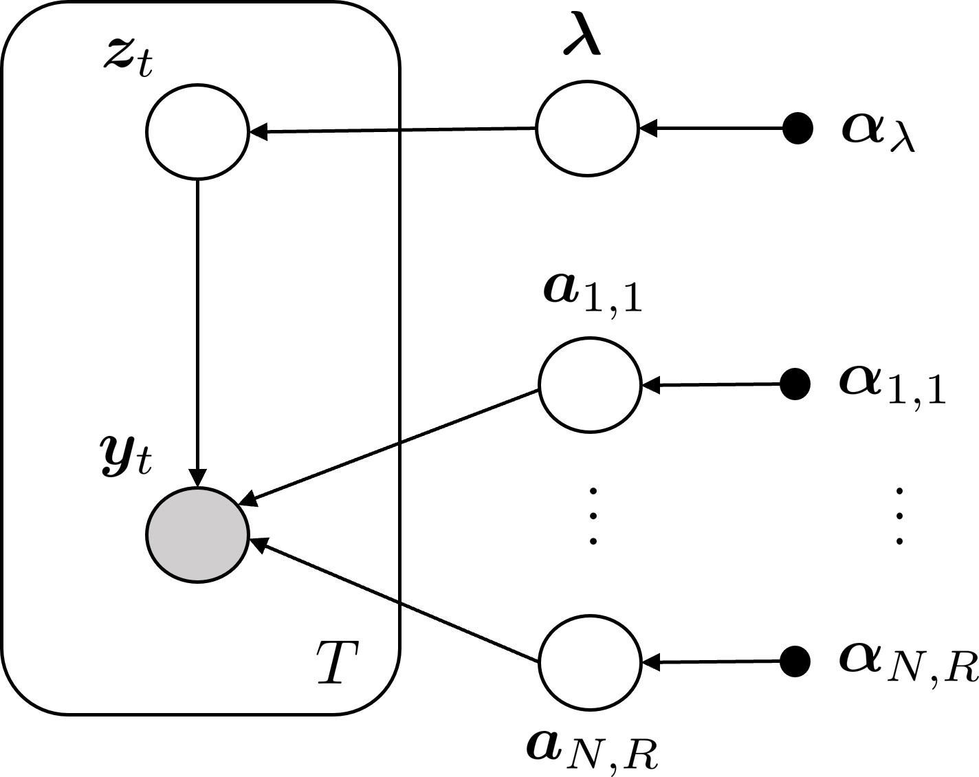
Figure 1: Probabilistic graphical model representation of the joint distribution $p(\bm{Y},\bm{\Theta})$.

$$p(\bm{Y},\bm{\Theta}) =p\big{(}\bm{Y}\,\big{|}\,\bm{Z},\{\bm{A}_{n}\}_{n=1}^{N}\big{)}\cdot p(\bm{Z}\,|\,\bm{\lambda})$$ (13)

$$\qquad\times p(\bm{\lambda})\cdot\prod_{n=1}^{N}\prod_{r=1}^{R}p(\bm{a}_{n,r}).$$

The probabilistic graphical model representation of $\eqref{eq:joint_distrib}$ is shown in Fig. 1. The latent variables $\{\bm{z}_{t}\}_{t=1}^{T}$ are said to be local parameters since $\bm{z}_{t}$ only governs the data in the $t$-th context. On the other hand, $\bm{\lambda}$ and $\bm{a}_{n,r},\forall n,r$, are global parameters since they are fixed in number independently of the size of the dataset.

The logarithm of the joint distribution is given by (cf. (5), (6), (11), and (12))

$$\log p(\bm{Y},\bm{\Theta}) =\sum_{t=1}^{T}\sum_{r=1}^{R}z_{r,t}\Big{(}\log\lambda_{r}+\sum_{n=1}^{N}\log a_{n,r,y_{n,t}}\Big{)}$$ (14)

$$+(\alpha_{\lambda}-1)\sum_{r=1}^{R}\log\lambda_{r}$$

$$+\sum_{n=1}^{N}\sum_{r=1}^{R}\sum_{i_{n}=1}^{I_{n}}(\alpha_{n,r}-1)\log a_{n,r,i_{n}}+\mathrm{const},$$

where ‘const’ refers to terms which do not depend on $\bm{Y}$ or $\bm{\Theta}$ and $a_{n,r,y_{n,t}}\triangleq\bm{A}_{n}(y_{n,t},r)$.

Our goal is to infer the posterior distribution $p(\bm{\Theta}\,|\,\bm{Y})$, i.e., the distribution of the unknown quantities given the observations. The classical approach is through Bayes theorem,

$$p(\bm{\Theta}\,|\,\bm{Y})=\frac{p(\bm{Y},\bm{\Theta})}{\int_{\bm{\Theta}}p(\bm{Y},\bm{\Theta})\mathrm{d}\bm{\Theta}}.$$ (15)

Exact inference requires integration over all variables in $\bm{\Theta}$ in order to calculate the denominator. In the present case, this is a high-dimensional problem involving integration over the model parameters and summation over all possible (discrete) states of the latent variables, which is computationally infeasible. In the following, we resort to approximate Bayesian inference which yields closed-form expressions for the posterior distribution.

III-B Posterior Approximation using Variational Inference

In variational inference (VI) [20], we seek a variational distribution $q(\bm{\Theta})$ that is closest to the true posterior distribution $p(\bm{\Theta}\,|\,\bm{Y})$ such that the Kullback-Leibler divergence (KLD) between them is minimized. The KLD is given by

$$D(q(\bm{\Theta})\,\|\,p(\bm{\Theta}\,|\,\bm{Y})) =\int_{\bm{\Theta}}q(\bm{\Theta})\log\frac{q(\bm{\Theta})}{p(\bm{\Theta}\,|\,\bm{Y})}\mathrm{d}\bm{\Theta}$$ (16)

$$=\log p(\bm{Y})-\underbrace{\int_{\bm{\Theta}}\bm{q}(\bm{\Theta})\log\frac{p(\bm{Y},\bm{\Theta})}{q(\bm{\Theta})}\mathrm{d}\bm{\Theta}}_{\mathcal{L}(q)}.$$

A closer examination of (16) reveals that since the KLD is nonnegative and the logarithm of the marginal likelihood $\log p(\bm{Y})$ is independent of $\bm{\Theta}$, then maximizing the term $\mathcal{L}(q)$ is equivalent to minimizing $D(q(\bm{\Theta})\,\|\,p(\bm{\Theta}\,|\,\bm{Y}))$. Therefore, $\mathcal{L}(q)$ is a lower bound on $\log p(\bm{Y})$ and is usually referred to as the evidence lower bound (ELBO).

If all possible variational distributions $q(\bm{\Theta})$ are considered, then the KLD vanishes when $q(\bm{\Theta})=p(\bm{\Theta}\,|\,\bm{Y})$. However, since the true posterior distribution is intractable, some restrictions need to be imposed on $q(\bm{\Theta})$ to ensure tractability. A common way to restrict the family of variational distributions is to assume that $q(\bm{\Theta})$ can be factorized such that $q(\bm{\Theta})=\prod_{i}q_{i}(\bm{\Theta}_{i})$, where $\cup_{i}\bm{\Theta}_{i}=\bm{\Theta}$ and $\cap_{i}\bm{\Theta}_{i}=\varnothing$. In other words, the unknown quantities in $\bm{\Theta}$ are assumed to be mutually independent with each quantity being governed by a distinct variational distribution. This approach is called mean-field approximation. In our case, given that $\bm{\Theta}=\{\bm{Z},\bm{\lambda},\bm{A}_{1},\dotsc,\bm{A}_{N}\}$, the mean-field approximation yields

$$q(\bm{\Theta})=\prod_{t=1}^{T}q_{z}(\bm{z}_{t})\cdot q_{\lambda}(\bm{\lambda})\cdot\prod_{n=1}^{N}\prod_{r=1}^{R}q_{n,r}(\bm{a}_{n,r}).$$ (17)

Under this setup, it can be shown that the optimal distribution $q_{i}^{\ast}(\bm{\Theta}_{i})$ for the $i$-th component of $q(\bm{\Theta})$ (i.e., the distribution for which $\mathcal{L}(q)$ is largest) is

$$\log q_{i}^{\ast}(\bm{\Theta}_{i})=\mathbb{E}_{q(\bm{\Theta}\backslash\bm{\Theta}_{i})}[\log p(\bm{Y},\bm{\Theta})]+\mathrm{const}.$$ (18)

Here, $\mathbb{E}_{q(\bm{\Theta}\backslash\bm{\Theta}_{i})}[\cdot]$ denotes the expectation with respect to ${q(\bm{\bm{\Theta}})}$ over all components except $\bm{\Theta}_{i}$, while $\log p(\bm{Y},\bm{\Theta})$ is given in (14). The constant is found by normalizing the distribution $q_{i}^{\ast}(\bm{\Theta}_{i})$, i.e.,

$$q_{i}^{\ast}(\bm{\Theta}_{i})=\frac{\exp\big{(}\mathbb{E}_{q(\bm{\Theta}\backslash\bm{\Theta}_{i})}[\log p(\bm{Y},\bm{\Theta})]\big{)}}{\int_{\bm{\Theta}_{i}}\exp\big{(}\mathbb{E}_{q(\bm{\Theta}\backslash\bm{\Theta}_{i})}[\log p(\bm{Y},\bm{\Theta})]\big{)}\mathrm{d}\bm{\Theta}_{i}}.$$ (19)

However, in most cases, the normalization constant will be readily apparent upon inspecting the resulting optimal distributions.

It can be seen from (18) that computing a particular variational distribution requires the knowledge of the other variational distributions. Therefore, the variational distributions are updated iteratively using a coordinate ascent algorithm (see Section III-D). In the following, we present the derivations of each variational distribution in (17).

III-B1 Posterior distribution $q^{\ast}_{\lambda}(\bm{\lambda})$ of the loading vector $\bm{\lambda}$

To derive $q^{\ast}_{\lambda}(\bm{\lambda})$, we first select, from (14), terms that depend on $\bm{\lambda}$ and then apply (18) by evaluating expectations over all other parameters (w.r.t. their respective $q(\cdot)$) except $\bm{\lambda}$. We have

$$\log q^{\ast}_{\lambda}(\bm{\lambda})=\sum_{r=1}^{R}\Big{(}\alpha_{\lambda}-1+\sum_{t=1}^{T}\mathbb{E}[z_{r,t}]\Big{)}\log\lambda_{r}+\mathrm{const}.$$ (20)

Taking exponentials on both sides reveals that

$$q^{\ast}_{\lambda}(\bm{\lambda})\propto\prod_{r=1}^{R}\lambda_{r}^{(\alpha_{\lambda}+\sum_{t=1}^{T}\mathbb{E}[z_{r,t}])-1},$$ (21)

which we immediately recognize as a Dirichlet distribution with parameters defined by

$$\widetilde{\alpha}_{\lambda,r}\triangleq\alpha_{\lambda}+\sum_{t=1}^{T}\mathbb{E}[z_{r,t}],~{}r=1,\dotsc,R.$$ (22)

Thus, the optimal variational distribution is given by

$$q_{\lambda}^{\ast}(\bm{\lambda})=\mathrm{Dir}(\bm{\lambda}\,|\,\widetilde{\bm{\alpha}}_{\lambda})=C(\widetilde{\bm{\alpha}}_{\lambda})\prod_{r=1}^{R}\lambda_{r}^{\widetilde{\alpha}_{\lambda,r}-1},$$ (23)

where $\widetilde{\bm{\alpha}}_{\lambda}=[\widetilde{\alpha}_{\lambda,1},\dotsc,\widetilde{\alpha}_{\lambda,R}]^{\mathsf{T}}$ are the global variational parameters (for the global parameter $\bm{\lambda}$) and $C(\widetilde{\bm{\alpha}}_{\lambda})$ is the normalization constant, which can be computed as in (8). A point estimate $\widehat{\bm{\lambda}}$ can be found by computing the posterior expectation over $q^{\ast}_{\lambda}(\bm{\lambda})$ (cf. (9)), i.e.,

$$\widehat{\lambda}_{r}=\mathbb{E}_{q_{\lambda}^{\ast}(\bm{\lambda})}[\lambda_{r}]=\frac{\widetilde{\alpha}_{\lambda,r}}{\sum_{j=1}^{R}\widetilde{\alpha}_{\lambda,j}},~{}r=1,\dotsc,R.$$ (24)

III-B2 Posterior distribution $q^{\ast}_{n,r}(\bm{a}_{n,r})$ of the factor matrix columns $\bm{a}_{n,r}$

From (14), we select terms with a dependence on $\bm{a}_{n,r}$ and then apply (18). This yields

$$\sum_{n=1}^{N}\sum_{r=1}^{R}\log q_{n,r}^{\ast}(\bm{a}_{n,r}) =\sum_{n=1}^{N}\sum_{r=1}^{R}\Bigg{(}\sum_{t=1}^{T}\mathbb{E}[z_{r,t}]\log a_{n,r,y_{n,t}}$$ (25)

$$+\sum_{i_{n}=1}^{I_{n}}(\alpha_{n,r}-1)\log a_{n,r,i_{n}}\Bigg{)}+\mathrm{const}.$$

In order to simplify (25), we need to introduce a summation over the index $i_{n}$ in the first term. Since $y_{n,t}\in\{1,\dotsc,I_{n}\}$, (25) can be equivalently expressed as

$$\sum_{n=1}^{N}\sum_{r=1}^{R}\log q_{n,r}^{\ast}(\bm{a}_{n,r}) =$$ (26)

$$\sum_{n=1}^{N}\sum_{r=1}^{R}\sum_{i_{n}=1}^{I_{n}}\Bigg{(}\Big{(}\sum_{t\in\Omega_{n,i_{n}}}\mathbb{E}[z_{r,t}]\Big{)}\log a_{n,r,i_{n}}$$

$$+(\alpha_{n,r}-1)\log a_{n,r,i_{n}}\Bigg{)}+\mathrm{const},$$

where $\Omega_{n,i_{n}}\triangleq\{t:y_{n,t}=i_{n}\}\subset\{1,\dotsc,T\}$ is the set of indices $t$ in which the observation $y_{n,t}$ equals the discrete value $i_{n}$. Restricting the summation range of the index $t$ in this way ensures that (26) and (25) are equivalent.

We can now isolate the $(n,r)$-th distribution, factor out $\log a_{n,r,i_{n}}$, and take exponentials on both sides, giving

$$q^{\ast}_{n,r}(\bm{a}_{n,r})\propto\prod_{i_{n}=1}^{I_{n}}a_{n,r,i_{n}}^{(\alpha_{n,r}+\sum_{t\in\Omega_{n,i_{n}}}\mathbb{E}[z_{r,t}])-1},~{}~{}\forall n,r.$$ (27)

This is also a Dirichlet distribution with parameters given by

$$\widetilde{\alpha}_{n,r,i_{n}}\triangleq\alpha_{n,r}+\sum_{t\in\Omega_{n,i_{n}}}\mathbb{E}[z_{r,t}],~{}i_{n}=1,\dotsc,I_{n}.$$ (28)

Thus, the optimal variational distribution is given by

$$q^{\ast}_{n,r}(\bm{a}_{n,r})=\mathrm{Dir}(\bm{a}_{n,r}\,|\,\bm{\alpha}_{n,r})=C(\widetilde{\bm{\alpha}}_{n,r})\prod_{i_{n}=1}^{I_{n}}a_{n,r,i_{n}}^{\widetilde{\alpha}_{n,r,i_{n}}-1},$$ (29)

where $\widetilde{\bm{\alpha}}_{n,r}=[\widetilde{\alpha}_{n,r,1},\dotsc,\widetilde{\alpha}_{n,r,I_{n}}]^{\mathsf{T}}$, $\forall n,r$, are the global variational parameters (for the global parameters $\bm{a}_{n,r}$) and $C(\widetilde{\bm{\alpha}}_{n,r})$ is the normalization constant, which can be computed as in (8). A point estimate $\widehat{\bm{a}}_{n,r}$ is found by computing the posterior expectation over $q^{\ast}_{n,r}(\bm{a}_{n,r})$ (cf. (9)), i.e.,

$$\widehat{a}_{n,r,i_{n}}=\mathbb{E}_{q^{\ast}_{n,r}(\bm{a}_{n,r})}[a_{n,r,i_{n}}]=\frac{\widetilde{\alpha}_{n,r,i_{n}}}{\sum_{j=1}^{I_{n}}\widetilde{\alpha}_{n,r,j}},~{}\forall i_{n}.$$ (30)

III-B3 Posterior distribution $q^{\ast}_{z}(\bm{z}_{t})$ of the latent variable $\bm{z}_{t}$

From (14), we select terms that have a dependence on $\bm{z}_{t}$ and then apply (18). We have

$$\log q^{\ast}_{z}(\bm{z}_{t})=\sum_{r=1}^{R}z_{r,t}\Big{(}\log\widetilde{\lambda}_{r}+\sum_{n=1}^{N}\log\widetilde{a}_{n,r,y_{n,t}}\Big{)}$$ (31)

where $\log\widetilde{x}\triangleq\mathbb{E}[\log x]$ and the expectations are taken with respect to the variational distributions $q^{\ast}_{\lambda}(\bm{\lambda})$ and $q^{\ast}_{n,r}(\bm{a}_{n,r})$, respectively. Therefore, the expectations are given by (cf. (10))

$$\log\widetilde{\lambda}_{r} =\psi(\widetilde{\alpha}_{\lambda,r})-\psi\Big{(}\sum_{j=1}^{R}\widetilde{\alpha}_{\lambda,r}\Big{)},$$ (32)

$$\log\widetilde{a}_{n,r,y_{n,t}} =\psi(\widetilde{\alpha}_{n,r,y_{n,t}})-\psi\Big{(}\sum_{j=1}^{I_{n}}\widetilde{\alpha}_{n,r,j}\Big{)}.$$

Taking exponentials on both sides of (31) yields

$$q^{\ast}_{z}(\bm{z}_{t})\propto\prod_{r=1}^{R}\gamma_{r,t}^{z_{r,t}},$$ (33)

where we have defined $\gamma_{r,t}$ as

$$\gamma_{r,t}\triangleq\exp\Big{\{}\log\widetilde{\lambda}_{r}+\sum_{n=1}^{N}\log\widetilde{a}_{n,r,y_{n,t}}\Big{\}}.$$ (34)

Normalizing (33) gives us the optimal variational distribution as

$$q^{\ast}_{z}(\bm{z}_{t})=\prod_{r=1}^{R}\rho_{r,t}^{z_{r,t}},$$ (35)

where

$$\rho_{r,t}\triangleq\frac{\gamma_{r,t}}{\sum_{j=1}^{R}\gamma_{j,t}}$$ (36)

is the local variational parameter (for the local parameter $z_{r,t}$). Recall that $\bm{z}_{t}$ is one-hot encoded (see Section III-A). Thus, taking the expectation with respect to (35) reveals that

$$\widehat{z}_{r,t}=\mathbb{E}_{q^{\ast}_{z}(\bm{z}_{t})}[z_{r,t}]=\rho_{r,t},$$ (37)

and this expectation can be inserted into (22) and (28) to compute the respective Dirichlet parameters.

Algorithm 1. VB-PMF Input: Dataset $\bm{Y}$, initial rank $R$ Output: CPD estimates $\widehat{\bm{\lambda}}$ and $\{\widehat{\bm{A}}_{n}\}_{n=1}^{N}$, rank estimate $\widehat{R}$ 1: Set prior hyperparameters $\alpha_{\lambda}$ and $\alpha_{n,r},\,\forall n,r$. 2: Initialize $\widetilde{\bm{\alpha}}_{\lambda}$ and $\widetilde{\bm{\alpha}}_{n,r},\forall n,r$ randomly. 3: repeat 4:     Update $\rho_{r,t},\,\forall r,t$ using (32), (34), and (36). 5:     Update $\widetilde{\alpha}_{\lambda,r},\,\forall r$ using (22). 6:     Update $\widetilde{\alpha}_{n,r,i_{n}},\,\forall n,r,i_{n}$ using (28). 7:     Evaluate the ELBO using (39). 8: until the ELBO converges 9: Find $\widehat{\bm{\lambda}}$ and $\{\widehat{\bm{A}}_{n}\}_{n=1}^{N}$ using (24) and (30), respectively. 10: Find $\widehat{R}$ by deleting components corresponding to $\quad\widehat{\lambda}_{r}<\epsilon$.

III-C Computing the ELBO

As mentioned earlier in Section III-B, the goal of variational inference is to find a distribution $q(\bm{\Theta})$ that is closest to the true posterior distribution $p(\bm{\Theta}\,|\,\bm{Y})$ in terms of the KLD. According to (16), instead of directly optimizing the KLD, we only need to maximize the ELBO $\mathcal{L}(q)$. Since $\mathcal{L}(q)$ is a lower bound, it should increase at each iteration during optimization and can therefore be used to evaluate the correctness of the mathematical expressions, as well as to test for convergence. From (16), the ELBO can be written as

$$\mathcal{L}(q)=\mathbb{E}_{q(\bm{\Theta})}[\log p(\bm{Y},\bm{\Theta})]-\mathbb{E}_{q(\bm{\Theta})}[\log q(\bm{\Theta})],$$ (38)

where the first term denotes the posterior expectation of the joint distribution (cf. (14)), while the second term is the (negative) entropy of the posterior distributions. The expectations are taken with respect to the optimal variational distributions in turn. For the first term in (38), the joint distribution $p(\bm{Y},\bm{\Theta})$ can be decomposed into various terms as shown in (13). Evaluating the expectations yields the closed-form expression in (39) for computing the ELBO. Details on the derivation of (39) can be found in the appendix.

 

$$\mathcal{L}(q) =\sum_{t=1}^{T}\sum_{r=1}^{R}\rho_{r,t}\Big{(}\log\widetilde{\lambda}_{r}+\sum_{n=1}^{N}\log\widetilde{a}_{n,r,y_{n,t}}\Big{)}+\sum_{n=1}^{N}\sum_{r=1}^{R}\Big{(}\log C(\bm{\alpha}_{n,r})+(\alpha_{n,r}-1)\sum_{i_{n}=1}^{I_{n}}\log\widetilde{a}_{n,r,i_{n}}\Big{)}$$ (39)

$$+\Big{(}\log C(\bm{\alpha}_{\lambda})+(\alpha_{\lambda}-1)\sum_{r=1}^{R}\log\widetilde{\lambda}_{r}\Big{)}-\sum_{t=1}^{T}\sum_{r=1}^{R}\rho_{r,t}\log\rho_{r,t}-\Big{(}\log C(\widetilde{\bm{\alpha}}_{\lambda})+\sum_{r=1}^{R}(\widetilde{\alpha}_{\lambda,r}-1)\log\widetilde{\lambda}_{r}\Big{)}$$

$$-\sum_{n=1}^{N}\sum_{r=1}^{R}\Big{(}\log C(\widetilde{\bm{\alpha}}_{n,r})+\sum_{i_{n}=1}^{I_{n}}(\widetilde{\alpha}_{n,r,i_{n}}-1)\log\widetilde{a}_{n,r,i_{n}}\Big{)}$$

III-D Algorithm: VB-PMF

The variational Bayesian PMF estimation procedure (VB-PMF) is outlined in Algorithm 1. The algorithm estimates the CPD components of the PMF tensor and also simultaneously and automatically infers the tensor rank. The automatic rank detection property arises from exploiting the sparsity-promoting properties of the Dirichlet distribution. Recall that the value of the Dirichlet parameter influences whether the resulting random variables are evenly or sparsely distributed within the probability simplex (see Section III-A). In particular, if the prior parameter $\alpha_{\lambda}$ is set to a small value close to 0 (e.g., $10^{-6}$), the point estimate $\widehat{\bm{\lambda}}$ obtained will be a sparse vector. This can be understood by noticing that (24) can be expressed as

$$\widehat{\lambda}_{r}=\frac{\alpha_{\lambda}+\sum_{t=1}^{T}\rho_{r,t}}{R\alpha_{\lambda}+T},$$ (40)

where we have used (22) and (37) together with the fact that $\sum_{t,r}\rho_{r,t}=T$. If the $r$-th component is not responsible for explaining the observations, then $\sum_{t}\rho_{r,t}\approx 0$. Therefore, for such a component, if $\alpha_{\lambda}\rightarrow 0$, then $\widehat{\lambda}_{r}\approx 0$ and the entire rank-one component (i.e., $\widehat{\lambda}_{r}$ and $\{\widehat{\bm{a}}_{n,r}\}_{n=1}^{N}$) can be pruned out of the model. The rank can therefore be determined via a single training run in which the algorithm is initialized with $R>R_{\mathrm{true}}$ components (where $R_{\mathrm{true}}$ is the unknown true rank of the PMF tensor), followed by pruning out components with a value less than some specified small positive constant $\epsilon$ after convergence. One strategy for choosing the initial number of components is to set $R$ to be the maximum possible rank for which the Kruskal uniqueness conditions for the CPD are satisfied [26], [27]. Alternatively, the initial rank can be set manually for computational efficiency. The algorithm is deemed to have converged when the difference between successive ELBO values is less than a specified threshold. Alternatively, instead of computing the ELBO of the full dataset, which could be expensive, the log-likelihood of a small held-out dataset can be used to test for convergence.

The complexity of the VB-PMF algorithm consists of updating the parameters of the variational distributions and computing the ELBO to check for convergence. The parameters $\rho_{r,t}$ are computed in $\mathcal{O}(NRT)$ while the combined complexity of computing $\widetilde{\bm{\alpha}}_{\lambda}$ and $\widetilde{\bm{\alpha}}_{n,r}$ is $\mathcal{O}(NR)$. In addition, the complexity of computing the ELBO is $\mathcal{O}(NRT)$. Thus, the overall complexity is $\mathcal{O}(NRT)$.

IV Scalable Bayesian PMF Estimation

In Section III, we have presented a PMF estimation approach based on variational Bayesian inference. One drawback of the VB-PMF algorithm is that, due to the coordinate ascent structure, the entire dataset needs to be analyzed at each iteration before updating the global variational parameters $\widetilde{\bm{\alpha}}_{\lambda}$ and $\widetilde{\bm{\alpha}}_{n,r}$. Thus, as the size of the dataset grows, VB-PMF does not scale well because each iteration becomes more computationally expensive. Scalability is especially important in the PMF estimation problem when the number of variables is large since a lot of data is required to obtain a reasonably accurate estimate of the joint PMF (even more if there are missing observations in the data). In this section, we present an improvement to VB-PMF which allows for scalability to massive datasets. The proposed algorithm is based on stochastic variational inference (SVI) [22], a method that scales variational inference by employing stochastic gradient-based optimization techniques in order to maximize the ELBO.

IV-A Preliminaries

We begin by briefly reviewing the exponential family of distributions (see, e.g., [1]). Given a random vector $\bm{x}\in\mathbb{R}^{n}$ governed by parameters $\bm{\theta}\in\mathbb{R}^{n}$, the exponential family of distributions over $\bm{x}$ given $\bm{\theta}$ is of the form

$$p(\bm{x}\,|\,\bm{\theta})=h(\bm{x})g(\bm{\theta})\exp\{\bm{\eta}\!^{\mathsf{T}}\!(\bm{\theta})\bm{u}(\bm{x})\},$$ (41)

where $h(\bm{x}):\mathbb{R}^{n}\mapsto\mathbb{R}$ is the base measure, $\bm{u}(\bm{x}):\mathbb{R}^{n}\mapsto\mathbb{R}^{n}$ are the sufficient statistics, $\bm{\eta}(\bm{\theta}):\mathbb{R}^{n}\mapsto\mathbb{R}^{n}$ are the natural parameters, and $g(\bm{\theta}):\mathbb{R}^{n}\mapsto\mathbb{R}$ is the normalization constant which ensures that $\int p(\bm{x}\,|\,\bm{\theta})\mathrm{d}\bm{x}=1$. Many of the most common probability distributions (e.g., normal, exponential, Bernoulli, Dirichlet, among others) are members of the exponential family. One attractive property of the exponential family is that certain moments can be easily calculated using differentiation. For instance, it can be shown that the expected value and the covariance of the sufficient statistics are given by

$$\mathbb{E}[\bm{u}(\bm{x})]=-\nabla\log g(\bm{\theta}),$$ (42)

$$\mathrm{cov}[\bm{u}(\bm{x}),\bm{u}(\bm{x})]=\nabla^{2}\log g(\bm{\theta}).$$ (43)

In addition, since $\bm{u}(\bm{x})$ are sufficient statistics, then (43) is also the Fisher information provided by the sample $\bm{x}$ about the parameter $\bm{\theta}$.

We are interested in using SVI to optimize the global variational parameters $\widetilde{\bm{\alpha}}_{\lambda}$ and $\widetilde{\bm{\alpha}}_{n,r}$, whose optimal variational distributions were found to be Dirichlet distributions (see (23) and (29)). It is useful to express the Dirichlet distribution in exponential form as such representation will come in handy in the sequel. Given a general Dirichlet distribution over a random vector $\bm{\mu}\in\mathbb{R}^{K}$ with parameters $\bm{\alpha}\in\mathbb{R}^{K}$, the exponential form is written as (cf. (7))

$$\mathrm{Dir}(\bm{\mu}\,|\,\bm{\alpha})=h(\bm{\mu})g(\bm{\alpha})\exp\{\bm{\eta}\!^{\mathsf{T}}\!(\bm{\alpha})\bm{u}(\bm{\mu})\},$$ (44)

with $h(\bm{\mu})=1$, $g(\bm{\alpha})=C(\bm{\alpha})$, $\bm{\eta}(\bm{\alpha})=[\alpha_{1}-1,\dotsc,\alpha_{K}-1]^{\mathsf{T}}$, and $\bm{u}(\bm{\mu})=[\log\mu_{1},\cdots,\log\mu_{K}]^{\mathsf{T}}$.

In the next subsection, we will use the exponential forms and the properties thereof to derive expressions for the natural gradient of the ELBO. These expressions will subsquently play an important role in the development of an SVI-based algorithm.

IV-B Computing the natural gradient of the ELBO

In classical gradient-based optimization where the goal is to maximize an objective function, the algorithm takes steps in the direction that results in the largest value for the function, but also maintains the shortest Euclidean distance between the steps (i.e., the direction of steepest ascent). However, the Euclidean distance does not capture the notion of (dis)similarity between probability distributions meaningfully; a more appropriate metric is the symmetric KLD, defined as $D(p\,\|\,q)+D(q\,\|\,p)$ for two distributions $p$ and $q$. Let the optimization problem be defined such that the steps taken minimize the symmetric KLD (as opposed to the Euclidean distance). The gradient which points in the direction of steepest ascent in the symmetric KLD metric space is termed the natural gradient [28].

Consider the parameter vector $\bm{\theta}$ defined in (41) and assume its assigned prior distribution is in the exponential family, i.e., $p(\bm{\theta}\,|\,\bm{\beta})=h(\bm{\theta})g(\bm{\beta})\exp\{\bm{\eta}\!^{\mathsf{T}}\!(\bm{\beta})\bm{u}(\bm{\theta})\}$. Suppose that we have approximated the true posterior distribution $p(\bm{\theta}\,|\,\bm{x})$ using a variational distribution $q^{\ast}_{\theta}(\bm{\theta}\,|\,\widetilde{\bm{\beta}})$. Our goal is to maximize the ELBO $\mathcal{L}(\widetilde{\bm{\beta}})$ over the variational parameter $\widetilde{\bm{\beta}}$. It has been shown in [22] that if $q^{\ast}_{\theta}(\bm{\theta}\,|\,\widetilde{\bm{\beta}})$ is in the exponential family, then the natural gradient of the ELBO is given by

$$\widetilde{\nabla}\mathcal{L}(\widetilde{\bm{\beta}})=\big{(}-\nabla^{2}\log g(\widetilde{\bm{\beta}})\big{)}^{-1}\cdot\nabla\mathcal{L}(\widetilde{\bm{\beta}}),$$ (45)

where $\nabla^{2}\log g(\widetilde{\bm{\beta}})$ is the Fisher information and $\nabla\mathcal{L}(\widetilde{\bm{\beta}})$ is the gradient of $\mathcal{L}(\widetilde{\bm{\beta}})$.

We are now ready to derive the natural gradients with respect to the global variational parameters $\widetilde{\bm{\alpha}}_{\lambda}$ and $\widetilde{\bm{\alpha}}_{n,r}$. The ELBO expressed as a function of $\widetilde{\alpha}_{\lambda,r}$ is given by (cf. (39))

$$\mathcal{L}(\widetilde{\alpha}_{\lambda,r})=\mathbb{E}[\log\lambda_{r}]\Bigg{(}\alpha_{\lambda}+\sum_{t=1}^{T}\rho_{r,t}-\widetilde{\alpha}_{\lambda,r}\Bigg{)}+\mathrm{const},$$ (46)

where we have explicitly written out the expected value in place of the notation $\log\widetilde{\lambda}_{r}$. Applying the exponential family property in (42) together with the general form in (44), we note that $\mathbb{E}[\log\lambda_{r}]=-\nabla_{{\widetilde{\alpha}_{\lambda,r}}}\log C(\widetilde{\bm{\alpha}}_{\lambda})$. Taking the gradient, we have

$$\nabla_{\widetilde{\alpha}_{\lambda,r}}\mathcal{L}{\color[rgb]{0,0,0}(\widetilde{\alpha}_{\lambda,r})}=-\nabla_{\widetilde{\alpha}_{\lambda,r}}^{2}\log C(\widetilde{\bm{\alpha}}_{\lambda})\Bigg{(}\alpha_{\lambda}+\sum_{t=1}^{T}\rho_{r,t}-\widetilde{\alpha}_{\lambda,r}\Bigg{)},$$ (47)

which is the gradient of the ELBO w.r.t the parameter $\widetilde{\alpha}_{\lambda,r}$. Finally, applying (45) with $\widetilde{\bm{\beta}}=\widetilde{\bm{\alpha}}_{\lambda}$ yields the natural gradient

$$\widetilde{\nabla}_{\widetilde{\alpha}_{\lambda,r}}\mathcal{L}{\color[rgb]{0,0,0}(\widetilde{\alpha}_{\lambda,r})}=\alpha_{\lambda}+\sum_{t=1}^{T}\rho_{r,t}-\widetilde{\alpha}_{\lambda,r},~{}\forall r.$$ (48)

By following a similar procedure, the natural gradient with respect to the parameter $\widetilde{\alpha}_{n,r,i_{n}}$ can also be found as

$$\widetilde{\nabla}_{\widetilde{\alpha}_{n,r,i_{n}}}\mathcal{L}{\color[rgb]{0,0,0}(\widetilde{\alpha}_{n,r,i_{n}})}=\alpha_{n,r}+\sum_{t\in\Omega_{n,i_{n}}}\rho_{r,t}-\widetilde{\alpha}_{n,r,i_{n}},~{}\forall n,r,i_{n}.$$ (49)

Notice the relationship between the natural gradients derived here and the variational update steps in (22) and (28), respectively. The natural gradient is therefore the difference between the variational updates and the current setting of the parameters.

Algorithm 2. SVB-PMF

Input: Dataset $\bm{Y}$, initial rank $R$, batch size $M$

Output: CPD estimates $\widehat{\bm{\lambda}}$ and $\{\widehat{\bm{A}}_{n}\}_{n=1}^{N}$, rank estimate $\widehat{R}$

1: Set prior hyperparameters $\alpha_{\lambda}$ and $\alpha_{n,r},\,\forall n,r$.

2: Initialize $\widetilde{\bm{\alpha}}_{\lambda}$ and $\widetilde{\bm{\alpha}}_{n,r},\forall n,r$ randomly.

3: repeat

4:     Randomly sample data points $\{\bm{y}_{t_{m}}\}_{m=1}^{M}$ from $\bm{Y}$.

5:     Update $\rho_{r,t_{m}},\,\forall r,t_{m}$ using (32), (34), and (36).

6:     Compute noisy gradients $\widehat{\nabla}_{\widetilde{\alpha}_{\lambda,r}}\mathcal{L}_{m}$ and

$\widehat{\nabla}_{\widetilde{\alpha}_{n,r,i_{n}}}\mathcal{L}_{m}$, $\forall m$ using (50) and (51), respectively.

7:     Compute the learning rates $\xi_{\lambda}$ and $\xi_{n,r},\forall n,r$

(e.g., (54)).

8:     Update $\widetilde{\alpha}_{\lambda,r},\,\forall r$ using (52).

9:     Update $\widetilde{\alpha}_{n,r,i_{n}},\,\forall n,r,i_{n}$ using (53).

10: until the log-likelihood of a held-out dataset converges.

11: Find $\widehat{\bm{\lambda}}$ and $\{\widehat{\bm{A}}_{n}\}_{n=1}^{N}$ using (24) and (30), respectively.

12: Find $\widehat{R}$ by deleting components corresponding to

$\quad\widehat{\lambda}_{r}<\epsilon$.

IV-C Stochastic optimization of the ELBO

The natural gradients in (48) and (49) can be used directly in a steepest ascent algorithm to maximize the ELBO. However, this approach would have the same computational complexity as the VB-PMF algorithm since it would require analyzing the entire dataset and computing the local variational parameters for each data point. This problem is solved using stochastic optimization, a technique which follows noisy estimates of the gradient in order to optimize an objective function. The noisy gradients are cheaper to compute since they are estimated by subsampling the data.

A noisy natural gradient is constructed by sampling $M\ll T$ data points at random, computing the natural gradient for each data point as though it was replicated $T$ times, and finally averaging over all $M$ data points in the minibatch. It was shown in [22] that this approach yields an unbiased estimate of the natural gradient. Let the random data points be $\{\bm{y}_{t_{1}},\dotsc,\bm{y}_{t_{M}}\}$, where $t_{m}\sim U(1,T)$ and $\bm{y}_{t_{m}}=[y_{1,t_{m}},\dotsc,y_{N,t_{m}}]^{\mathsf{T}}$ for $m=1,\dotsc,M$. Thus, proceeding from (48) and (49), the noisy natural gradients of the ELBO as a function of the global variational parameters $\widetilde{\bm{\alpha}}_{\lambda}$ and $\widetilde{\bm{\alpha}}_{n,r}$ at the $m$-th data point and the $k$-th iteration are given by

$$\widehat{\nabla}_{\widetilde{\alpha}^{(k)}_{\lambda,r}}\mathcal{L}_{m}=\alpha_{\lambda}+T\rho^{(k)}_{r,t_{m}}-\widetilde{\alpha}^{(k-1)}_{\lambda,r},$$ (50)

$$\widehat{\nabla}_{\widetilde{\alpha}^{(k)}_{n,r,i_{n}}}\mathcal{L}_{m}=\alpha_{n,r}+I\{y_{n,t_{m}}=i_{n}\}T\rho^{(k)}_{r,t_{m}}-\widetilde{\alpha}^{(k-1)}_{n,r,i_{n}},$$ (51)

where the indicator function $I\{\cdot\}$ yields 1 when $y_{n,t_{m}}=i_{n}$ and 0 otherwise.

These noisy gradients can now be used in a steepest ascent algorithm. For the $k$-th iteration, we have the following updates

$$\widetilde{\alpha}_{\lambda,r}^{(k)}=\widetilde{\alpha}_{\lambda,r}^{(k-1)}+\xi^{(k)}_{\lambda}\Bigg{(}\frac{1}{M}\sum_{m=1}^{M}\widehat{\nabla}_{\widetilde{\alpha}_{\lambda,r}^{(k)}}\mathcal{L}_{m}\Bigg{)},$$ (52)

$$\widetilde{\alpha}_{n,r,i_{n}}^{(k)}=\widetilde{\alpha}_{n,r,i_{n}}^{(k-1)}+\xi^{(k)}_{n,r}\Bigg{(}\frac{1}{M}\sum_{m=1}^{M}\widehat{\nabla}_{\widetilde{\alpha}_{n,r,i_{n}}^{(k)}}\mathcal{L}_{m}\Bigg{)},$$ (53)

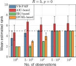
(a)

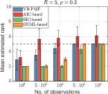
(b)

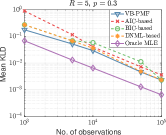
(c)

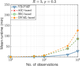
(d)

Figure 2: Joint PMF estimation and rank detection for different number of observations $T$. The true rank of the PMF tensor is $R=5$. (a) Mean estimated rank ($p=0$); (b) Mean estimated rank ($p=0.3$); (c) Mean KLD between the estimated and true PMF tensors ($p=0.3$); (d) Mean runtime ($p=0.3$).

where $\xi^{(k)}_{\lambda}$ and $\xi^{(k)}_{n,r}$ are the learning rates for $\widetilde{\bm{\alpha}}_{\lambda}$ and $\widetilde{\bm{\alpha}}_{n,r}$, respectively. To guarantee convergence, both learning rate sequences should be chosen to satisfy the Robbins-Monro conditions [29], i.e., $\sum_{k}\xi^{(k)}=\infty$ and $\sum_{k}\xi^{(k)^{2}}<\infty$. Alternatively, the authors in [30] have proposed a method to compute the learning rate adaptively, based on minimizing the expected squared norm of the error between the stochastic updates (e.g., (52)) and the optimal variational parameters (e.g., (22)). The learning rate requires no hand-tuning and performs better than the former approach. Therefore, we adopt the method in [30] to compute the learning rates. As an example, the learning rate for the update of $\widetilde{\bm{\alpha}}_{\lambda}$ is computed as follows (a similar procedure holds for $\widetilde{\bm{\alpha}}_{n,r}$). Let $\bm{g}^{(k)}\in\mathbb{R}^{R}$ contain the noisy natural gradients defined in (50) for all $r$. Then, the learning rate at the $k$-th iteration is given by [30]

$$\xi_{\lambda}^{(k)}=\frac{\mathbb{E}[\bm{g}^{(k)}]^{\mathsf{T}}\cdot\mathbb{E}[\bm{g}^{(k)}]}{\mathbb{E}[\bm{g}^{(k)^{\mathsf{T}}}\bm{g}^{(k)}]}\approx\frac{\overline{\bm{g}}^{(k)^{\mathsf{T}}}\overline{\bm{g}}^{(k)}}{\overline{\bm{h}}^{(k)}},$$ (54)

where the expected values $\mathbb{E}[\bm{g}^{(k)}]$ and $\mathbb{E}[\bm{g}^{(k)^{\mathsf{T}}}\bm{g}^{(k)}]$ are approximated by their respective exponential moving averages $\overline{\bm{g}}^{(k)}$ and $\overline{\bm{h}}^{(k)}$.

The complete algorithm, which we call stochastic VB-PMF (SVB-PMF), is summarized in Algorithm 2. The algorithm has a number of attractive properties. Firstly, all the quantities that need to be computed in SVB-PMF are already in place once VB-PMF is implemented, thus VB-PMF can be converted into its stochastic counterpart without much effort. Secondly, as pointed out earlier, the key advantage of the stochastic approach is scalability as the size of the dataset increases. The overall complexity of the algorithm is $\mathcal{O}(NRM)$, where $M$ is the batch size. Thus, if the batch size is chosen such that $M$ has a sub-linear dependence on $T$ (e.g., $M=T^{1/b},b>1$), considerable savings in computation time can be achieved.

V Results

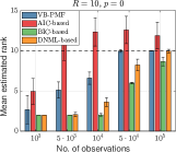
(a)

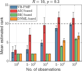
(b)

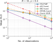
(c)

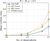
(d)

Figure 3: Joint PMF estimation and rank detection for different number of observations $T$. The true rank of the PMF tensor is $R=10$. (a) Mean estimated rank ($p=0$); (b) Mean estimated rank ($p=0.3$); (c) Mean KLD between the estimated and true PMF tensors ($p=0.3$); (d) Mean runtime ($p=0.3$).

In this section, we evaluate the performance of the proposed Bayesian estimation algorithms through carefully designed synthetic data simulations. In addition, both approaches are applied to movie recommendation data to demonstrate their effectiveness in real statistical learning tasks.

V-A Synthetic-Data Experiments

V-A1 VB-PMF performance

We consider a small-scale experiment with $N=5$ discrete random variables each taking $I_{n}=10$ states. We assume that the 5-dimensional joint PMF tensor $\bm{\mathcal{X}}$ admits a naïve Bayes model. The number of states that the hidden variable $H$ can take is set to $R=\{5,10\}$. The elements of $\bm{\lambda}\in\mathbb{R}^{R}$ and $\{\bm{A}_{n}\}_{n=1}^{N}\in\mathbb{R}^{I_{n}\times R}$ are drawn randomly from $U(0.3,1)$ and $U(0,1)$, respectively, followed by normalization according to the probability simplex constraints. The tensor $\bm{\mathcal{X}}$ is then constructed according to (2) and is fixed for the rest of the experiment. For each trial, a dataset $\bm{Y}\in\mathbb{R}^{N\times T}$ containing observations $\bm{y}_{t}$ is obtained by first sampling $\bm{x}_{t}$ from $\bm{\mathcal{X}}$ (according to the naïve Bayes model), then randomly and independently zeroing out its elements according to the outage probability $p$ (cf. Section II). The values of the outage probability are set to $p=\{0,0.3\}$. The accuracy of the estimate is evaluated in terms of the KLD

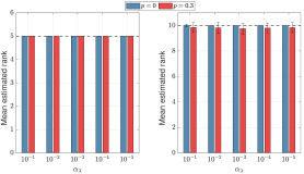
Figure 4: VB-PMF rank estimation performance under various values of the hyperparameter $\alpha_{\lambda}$ for true ranks $R=5$ (left) and $R=10$ (right). Here, $T=10^{5}$ and the outage probabilities are $p=\{0,0.3\}$.

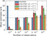
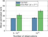
Figure 5: SVB-PMF rank estimation performance versus the number of observations $T$ under various minibatch sizes $M$. The true rank is $R=25$. Left: Maximum runtime allowed is 10 hours with the convergence threshold set to $10^{-7}$. Right: Maximum runtime allowed is 15 hours with the convergence threshold set to zero.

between the true PMF $\bm{\mathcal{X}}$ and the estimated PMF $\widehat{\bm{\mathcal{X}}}$, computed as

$$D(\bm{\mathcal{X}}\,\|\,\widehat{\bm{\mathcal{X}}})=\sum_{i_{1},\dotsc,i_{N}}\bm{\mathcal{X}}(i_{1},\dotsc,i_{N})\log\frac{\bm{\mathcal{X}}(i_{1},\dotsc,i_{N})}{\widehat{\bm{\mathcal{X}}}(i_{1},\dotsc,i_{N})}.$$

The performance of VB-PMF is compared with three model selection techniques for naïve Bayes models [15]: the Akaike information criterion (AIC), the Bayesian information criterion (BIC), and the decomposed normalized maximum likelihood (DNML) criterion. These techniques require cross-validation in order to find the best rank. To estimate the CPD components, we use SQUAREM-PMF [12], an accelerated form of the expectation maximization (EM) algorithm [11], and test candidate ranks in the range $\{1,\dotsc,R+5\}$. We initialize VB-PMF with $R=23$ components and set the hyperparameters $\alpha_{\lambda}$ and $\alpha_{n,r}$ to $10^{-6}$ and $1$, respectively. This hyperparameter setting favors sparse solutions for $\bm{\lambda}$ and all possible solutions for $\{\bm{A}_{n}\}_{n=1}^{N}$, allowing the rank to be estimated as part of the inference. In addition, the pruning threshold is set to $\epsilon=10^{-3}$

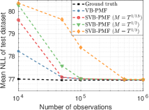
Figure 6: Mean negative log-likelihood (NLL) of a held-out test dataset versus the number of observations $T$. Three SVB-PMF variants with different minibatch sizes $M$ are shown.

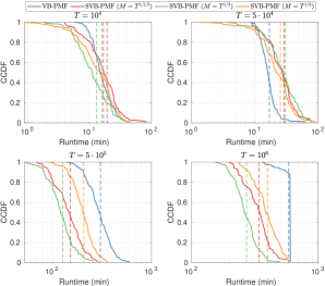
Figure 7: Complementary cumulative distribution function (CCDF) of the runtime for different number of observations $T$. The vertical dashed lines indicate the mean runtime. Maximum allowed runtime is 10 hours with the convergence threshold set to $10^{-7}$.

while the convergence thresholds for both SQUAREM-PMF and VB-PMF are set to $10^{-7}$.

Figs. 2 and 3 presents results (averaged over 100 independent trials) for a rank-$5$ and a rank-$10$ PMF tensor, respectively. For both outage values $p=\{0,0.3\}$, the rank inferred by VB-PMF converges to the true rank as the number of observations is increased. A similar observation can be made for BIC and DNML. However, for $R=10$ and $p=0.3$, BIC and DNML are not able to detect the correct rank and would need much more data to do so. On the other hand, AIC exhibits a large variance in the inferred rank, which is unsurprising as AIC is not a consistent criterion [31]. In terms of the accuracy, VB-PMF performs comparably to or better than the other model order estimation techniques. Here, the ‘Oracle’ ML estimate (MLE), which assumes that the true hidden state associated with each observation is known, serves as an empirical lower bound for the KLD. This result can be attributed to the fact that VB-PMF detects the correct rank with minimal or no misfit as the size of the dataset increases. Moreover, the runtime plots show that VB-PMF provides significant gains in computational efficiency as the size of the dataset grows, even though the runtime increases linearly with the dataset size. This is because the rank is estimated via a single training run, while the other model order selection techniques need multiple training runs over the candidate ranks.

Fig. 4 shows the rank estimation performance as a function of the loading vector hyperparameter $\alpha_{\lambda}$. The estimated rank is consistent regardless of the choice of $\alpha_{\lambda}$. It is only required that $\alpha_{\lambda}\ll 1$ in order to obtain a sparse loading vector for rank inference. As mentioned earlier, in the absence of prior information, it is reasonable to set $\alpha_{n,r}=1$ in order to allow all possible solutions for the factor matrix columns. This result demonstrates the robustness of VB-PMF to the choice of the hyperparameter $\alpha_{\lambda}$.

V-A2 SVB-PMF performance

TABLE I: Performance of different algorithms on the MovieLens dataset.

Estimation algorithm	Model order selection criterion	RMSE	MAE	NLL	Most common CPD rank	Mean runtime (hrs)
VB-PMF (proposed)	-	$\mathbf{0.726\pm 0.005}$	$\mathbf{0.540\pm 0.003}$	$\mathbf{20.543\pm 0.080}$	$44$	$3.17$
SVB-PMF (proposed)	-	$0.737\pm 0.006$	$0.551\pm 0.004$	$20.594\pm 0.082$	$31$	$\mathbf{0.52}$
SQUAREM-PMF [12]	ValErr	$0.731\pm 0.005$	$0.544\pm 0.003$	$20.552\pm 0.083$	$30$	$21.27$
	AIC [13]	$0.732\pm 0.006$	$0.544\pm 0.004$	$20.553\pm 0.079$	$30$	$59.53$
	BIC [14]	$0.790\pm 0.010$	$0.592\pm 0.008$	$20.727\pm 0.083$	$10$	$59.53$
	DNML [15]	$0.759\pm 0.010$	$0.567\pm 0.008$	$20.638\pm 0.088$	$15$	$59.98$
CTF3D [5]	ValErr	$0.846\pm 0.020$	$0.617\pm 0.022$	$21.838\pm 0.139$	$30$	$41.55$
BMF [32]	ValErr	$0.958\pm 0.006$	$0.740\pm 0.004$	-	-	-

Next, we consider a larger problem with $N=50$ discrete random variables each taking $I_{n}=10$ states and with rank $R=25$. The outage probability is set to $p=0.3$. As before, the elements of $\bm{\lambda}$ and $\{\bm{A}_{n}\}_{n=1}^{N}$ are drawn from $U(0.3,1)$ and $U(0,1)$, respectively, and normalized to fulfill the probability simplex constraints.

We investigate three choices for the SVB-PMF minibatch size $M$. In particular, since we would like the asymptotic complexity of SVB-PMF to be sublinear in $T$, we set $M=T^{1/b}$, where $b\in\{1.5,2,3\}$. The performance of SVB-PMF is compared with that of VB-PMF. For both algorithms, the hyperparameters are set to $\alpha_{\lambda}=10^{-6}$ and $\alpha_{n,r}=1$, the pruning threshold is set to $\epsilon=10^{-3}$, and the initial rank is $R=50$. Furthermore, $10\%$ of the observations are held out as a test dataset to check for convergence. The results are averaged over 100 independent trials.

In Fig. 5, we present the mean estimated rank as a function of the number of observations $T$ in the dataset. For $T=10^{4}$, all algorithms are unable to determine the correct model order due to an insufficient number of samples. As $T$ is increased, we observe that VB-PMF accurately determines the model order. On the other hand, while SVB-PMF benefits from larger minibatch sizes for intermediate values of $T$, overfitting is observed for $T=\{5\cdot 10^{5},{\color[rgb]{0,0,0}10^{6}}\}$, although to a reduced extent for the smallest minibatch size, $M=T^{1/3}$. The overfitting in our experiments arises as a result of imposing a maximum allowed runtime for both algorithms, as well as a convergence threshold. Higher accuracy can be obtained by increasing the maximum allowed runtime and/or decreasing the convergence threshold. The plot on the right in Fig. 5 shows a reduction in overfitting for both algorithms when the maximum allowed runtime is increased from 10 hours to 15 hours with the convergence threshold set to zero.

To gain further insight, we study the mean negative log-likelihood (NLL) of the held-out test dataset, which serves as an indicator of the quality of the learned model. As shown in Fig. 7, the mean NLL for all three SVB-PMF variants approaches the ground truth as $T$ increases, with larger minibatch sizes leading to faster convergence. Even though there is some overfitting for $T=\{5\cdot 10^{5},10^{6}\}$ (see Fig. 5), the effect on the quality of the model is quite minimal.

Finally, in Fig. 7, we present the distribution of the runtime for each value of $T$. For $T=10^{4}$, both VB-PMF and SVB-PMF have roughly equivalent runtimes, while VB-PMF is more computationally efficient for $T=5\cdot 10^{4}$. For moderately large values of $T$, VB-PMF is able to converge faster by analyzing the entire dataset, while SVB-PMF takes longer due to the minibatch operation. However, for $T=\{5\cdot 10^{5},10^{6}\}$, the linear dependence of VB-PMF on $T$ starts to become a bottleneck and the computational advantage of SVB-PMF is readily apparent. Note that even though one could argue that such a large dataset is not required in this case (cf. Fig. 7), in a real-world scenario, the true PMF (and, hence, the true NLL) is unknown. Therefore, it would be difficult to know in advance how much data is required for a good estimate.

V-B Real-Data Experiments

We evaluate the performance of the proposed algorithms in a real-world movie recommendation application. For this purpose, we utilize the MovieLens 25M dataset [33] which contains 25 million movie ratings on a 5-star scale with half-star increments, i.e., $\{0.5,\dotsc,5.0\}$. From the entire dataset, we select the ratings of $N=50$ top-rated movies. We perform some pre-processing by omitting users who have rated only one or none of the selected movies and mapping the ratings to a discrete scale $\{1,\dotsc,10\}$. Thus, we obtain a movie-user rating matrix $\bm{Y}\in\mathbb{R}^{N\times T}$ where the number of users $T=1.{\color[rgb]{0,0,0}5}2\times 10^{5}$. The percentage of missing ratings in the rating matrix is about 67% (outage probability $p=0.67$). Moreover, since we are dealing with real data, the true rank (model order) is unknown.

Our aim is to estimate the joint PMF (i.e., $\{\bm{A}_{n}\}_{n=1}^{N}$ and $\bm{\lambda}$) of the ratings from the observations in order to predict missing ratings. In this scenario, the joint PMF to be estimated is a 50-dimensional tensor $\bm{\mathcal{X}}\in\mathbb{R}^{I_{1}\times\cdots\times I_{N}}$ with each dimension $I_{n}=10$, $n=1,\dotsc,50$. We run 20 Monte Carlo trials whereby 70% of the ratings are used to estimate the joint PMF, 10% serve as a validation set for model order selection (choosing the CPD rank) or to check for convergence, and 20% are used for testing the algorithms. In each trial, a different training/validation/testing split is applied to the rating matrix.

The proposed algorithms, VB-PMF and SVB-PMF, require no cross-validation for model order selection. Hence, in both cases, the NLL of the validation set is used to test for convergence. Both algorithms are initialized with $R=50$ components and the hyperparameters $\alpha_{\lambda}$ and $\alpha_{n,r}$ are set to $10^{-6}$ and $1$, respectively. The batch size for SVB-PMF is set to $M=500$ ($\approx T^{1/2}$). For comparison, we include AIC, BIC, and DNML, for which the best model order is chosen based on the respective criterion evaluated on the training set. We also include ValErr, for which the best model order is chosen based on the root mean square error (RMSE) of the validation set, as is the standard practice in the machine learning literature. The estimation algorithm for these four techniques is SQUAREM-PMF [12] (cf. Section V-A). We also include coupled tensor factorization based on 3D marginals (CTFD) [5] as a benchmark for PMF estimation algorithms. For computational efficiency, the set of candidate ranks was restricted to $\{5,10,15,20,25,30\}$. These PMF-based approaches are compared with biased matrix factorization (BMF) [32] which is a classical technique for recommendation systems.

During the testing phase (also during validation for the ValErr approach), for each test sample, one rating is hidden and predicted using the estimated PMF from each approach. The predicted rating is found by computing its conditional expectation with respect to the estimated joint PMF. In particular, let the current test sample be $\bm{y}_{t}=[y_{1,t},\dotsc,y_{N,t}]^{\mathsf{T}}$ and suppose that $y_{N,t}=0$, i.e., hidden. The predicted rating is then

$$\hat{y}_{N,t}=\sum_{i_{N}=1}^{I_{N}}i_{N}\mathsf{Pr}(i_{N}\,|\,y_{1,t},\dotsc,y_{N-1,t}),$$ (55)

where the conditional PMF can be computed from the joint PMF via Bayes’ theorem. The quality of the predictions is evaluated by computing the RMSE and the mean absolute error (MAE) between the predicted and true ratings. Moreover, the mean NLL of the test dataset is presented as a means of comparing the overall quality of the models (the lower the better).

Table I presents the performance of the various PMF estimation algorithms in terms of the RMSE, the MAE and the mean NLL. In addition, we also report the most common (estimated) rank as well as the mean runtime. It can be observed that VB-PMF achieves the best performance across all metrics. In comparison, SVB-PMF experiences some performance loss. This result is expected since SVB-PMF operates on minibatches of data while VB-PMF processes the entire dataset. However, SVB-PMF yields remarkable savings in the computation time compared to VB-PMF, and thus the marginal degradation in accuracy can be tolerated. As expected, there is a huge computational cost incurred by SQUAREM-PMF and CTF3D due to model order selection, although SQUAREM-PMF performs comparably to the Bayesian algorithms in some cases. Note that the number of candidate ranks for SQUAREM-PMF and CTF3D was restricted for computational efficiency; our approaches would be even more advantageous if more candidate ranks were considered. Compared to the other PMF estimation algorithms, CTF3D experiences performance degradation due to the restriction to only use 3D marginals. In terms of the RMSE and the MAE, all PMF estimation algorithms outperform BMF. This result demonstrates that the estimated joint PMF tensor captures the user-movie interactions more accurately than the matrix factorization techniques on which BMF is based.

Finally, we attempt to provide some interpretation regarding the most common (estimated) ranks. The rank of the PMF tensor is the number of states that the latent variable in the naïve Bayes model can take (cf. Section II). Since the true rank is unknown, it is difficult to determine how good the estimates are. However, the performance metrics provide at least an indication of the quality of the rank estimates. In particular, VB-PMF infers the largest rank and achieves the best performance. Similarly, the performance of SVB-PMF and SQUAREM-PMF (with model selection criteria ValErr and AIC) is comparable, and so are the inferred/selected ranks. The BIC and DNML selection criteria result in much lower ranks with an accompanying performance degradation. These observations could be explained by remarking that the rank is connected to the complexity of the learned model, i.e., how well the model can capture the underlying patterns in the data. Note that VB-PMF and SVB-PMF were initialized with relatively complex models having rank $R=50$. Both algorithms then inferred simpler models with sufficient complexity. However, VB-PMF learned a more complex model compared to SVB-PMF by processing the entire dataset in each iteration.

VI Conclusion

In this work, we have presented a Bayesian PMF estimation approach that simultaneously allows the rank (model order) of the joint PMF tensor to be inferred from observed data. Our approach only requires a single training run in order to infer the rank, obviating the need for computationally intensive cross-validation procedures typical of classical model order selection techniques. Moreover, we have developed a scalable version of the PMF estimation approach which leverages stochastic optimization techniques, enabling efficient handling of massive datasets with minimal performance loss. Numerical simulations on synthetic data have demonstrated the validity of our approaches in terms of computational efficiency, robustness to missing data, tuning-free rank inference, and scalability. Additionally, results from a real-world experiment demonstrate that our proposed algorithms outperform state-of-the-art techniques in both accuracy and computational efficiency, further highlighting their practical applicability.

Derivation of the ELBO

We begin by expanding the first term on the right-hand side of (38) into its constituent distributions. This gives (cf. (13))

$$\mathbb{E}[\log p(\bm{Y}\,|\bm{\Theta})] =$$ (56)

$$\mathbb{E}\Big{[}\log p\big{(}\bm{Y}\,\big{|}\,\bm{Z},\{\bm{A}_{n}\}_{n=1}^{N}\big{)}\Big{]}+\mathbb{E}\Big{[}\log p(\bm{Z}\,|\,\bm{\lambda})\Big{]}$$

$$+\mathbb{E}\Big{[}\log p(\bm{\lambda})\Big{]}+\sum_{n=1}^{N}\sum_{r=1}^{R}\mathbb{E}\Big{[}\log p(\bm{a}_{n,r})\Big{]},$$

where the explicit dependence of the expected values on the variational distributions $q(\cdot)$ has been dropped for brevity. Next, we substitute for each distribution and take the expected value of each parameter with respect to its variational distribution in turn. Thus (cf. (14)),

$$\mathbb{E}\Big{[}\log p\big{(}\bm{Y}\,\big{|}\,\bm{Z},\{\bm{A}_{n}\}_{n=1}^{N}\big{)}\Big{]}+\mathbb{E}\Big{[}\log p(\bm{Z}\,|\,\bm{\lambda})\Big{]}$$

$$=\sum_{t=1}^{T}\sum_{r=1}^{R}\mathbb{E}[z_{r,t}]\Big{(}\mathbb{E}\big{[}\log\lambda_{r}\big{]}+\sum_{n=1}^{N}\mathbb{E}\big{[}\log a_{n,r,y_{n,t}}\big{]}\Big{)}$$ (57)

$$\mathbb{E}\Big{[}\log p(\bm{\lambda})\Big{]} =\log C(\bm{\alpha}_{\lambda})+(\alpha_{\lambda}-1)\sum_{r=1}^{R}\mathbb{E}[\log\lambda_{r}]$$ (58)

$$\mathbb{E}\Big{[}\log p(\bm{a}_{n,r})\Big{]} =\log C(\bm{\alpha}_{n,r})$$

$$+(\alpha_{n,r}-1)\sum_{i_{n}=1}^{I_{n}}\mathbb{E}[\log a_{n,r,i_{n}}]$$ (59)

Solving the expectations using (32) and (37) yields the first three terms of (39). Similarly, the second term on the right-hand side of (38) is given by (cf. (17))

$$\mathbb{E}[\log q(\bm{\Theta})] =\sum_{t=1}^{T}\mathbb{E}[\log q_{z}(\bm{z}_{t})]+\mathbb{E}[\log q_{\lambda}(\bm{\lambda})]$$ (60)

$$+\sum_{n=1}^{N}\sum_{r=1}^{R}\mathbb{E}[\log q_{n,r}(\bm{a}_{n,r})].$$

Substituting for the variational distributions gives (cf. (35), (23), and (29))

$$\mathbb{E}[\log q_{z}(\bm{z}_{t})] =\sum_{r=1}^{R}\mathbb{E}[z_{r,t}]\log\rho_{r,t}$$ (61)

$$\mathbb{E}[\log q_{\lambda}(\bm{\lambda})] =\log C(\widetilde{\bm{\alpha}}_{\lambda})+(\widetilde{\alpha}_{\lambda}-1)\mathbb{E}[\log\lambda_{r}]$$ (62)

$$\mathbb{E}[\log q_{n,r}(\bm{a}_{n,r})] =\log C(\widetilde{\bm{\alpha}}_{n,r})$$

$$+(\widetilde{\alpha}_{n,r}-1)\sum_{i_{n}=1}^{I_{n}}\mathbb{E}[\log a_{n,r,i_{n}}]$$ (63)

after which the expectations are solved via (32) and (37) to yield the last three terms of (39).

References

- [1] C. M. Bishop, Pattern Recognition and Machine Learning (Information Science and Statistics). Berlin, Heidelberg: Springer-Verlag, 2006.
- [2] T. G. Kolda and B. W. Bader, “Tensor Decompositions and Applications,” SIAM Rev., vol. 51, no. 3, pp. 455–500, Aug. 2009.
- [3] N. D. Sidiropoulos, L. De Lathauwer, X. Fu, K. Huang, E. E. Papalexakis, and C. Faloutsos, “Tensor Decomposition for Signal Processing and Machine Learning,” IEEE Transactions on Signal Processing, vol. 65, no. 13, pp. 3551–3582, Jul. 2017.
- [4] M. Ishteva, “Tensors and Latent Variable Models,” in Latent Variable Analysis and Signal Separation, E. Vincent, A. Yeredor, Z. Koldovský, and P. Tichavský, Eds., 2015, pp. 49–55.
- [5] N. Kargas, N. D. Sidiropoulos, and X. Fu, “Tensors, Learning, and “Kolmogorov Extension” for Finite-Alphabet Random Vectors,” IEEE Trans. Signal Process., vol. 66, no. 18, pp. 4854–4868, Sep. 2018.
- [6] M. Amiridi, N. Kargas, and N. D. Sidiropoulos, “Statistical Learning Using Hierarchical Modeling of Probability Tensors,” in Proc. IEEE Data Science Workshop (DSW), Jun. 2019.
- [7] A. Yeredor and M. Haardt, “Estimation of a Low-Rank Probability-Tensor from Sample Sub-Tensors via Joint Factorization Minimizing the Kullback-Leibler Divergence,” in Proc. 27th IEEE European Signal Processing Conference (EUSIPCO), A Coruna, Spain, Sep. 2019.
- [8] S. Ibrahim and X. Fu, “Recovering Joint Probability of Discrete Random Variables from Pairwise Marginals,” IEEE Transactions on Signal Processing, 2021.
- [9] J. Vora, K. S. Gurumoorthy, and A. Rajwade, “Recovery of Joint Probability Distribution from One-Way Marginals: Low Rank Tensors and Random Projections,” in Proc. IEEE Statistical Signal Processing Workshop (SSP), Jul. 2021.
- [10] P. Flores, G. Harle, A.-B. Notarantonio, K. Usevich, M. D’Aveni, S. Grandemange, M.-T. Rubio, and D. Brie, “Coupled Tensor Factorization for Flow Cytometry Data Analysis,” in Proc. 32nd IEEE International Workshop on Machine Learning for Signal Processing (MLSP), Xi’an, China, Aug. 2022.
- [11] A. Yeredor and M. Haardt, “Maximum Likelihood Estimation of a Low-Rank Probability Mass Tensor From Partial Observations,” IEEE Signal Process. Lett., vol. 26, no. 10, pp. 1551–1555, Oct. 2019.
- [12] J. K. Chege, M. J. Grasis, A. Manina, A. Yeredor, and M. Haardt, “Efficient Probability Mass Function Estimation from Partially Observed Data,” in Proc. 56th IEEE Asilomar Conference on Signals, Systems, and Computers, Oct. 2022.
- [13] H. Akaike, “A New Look at the Statistical Model Identification,” IEEE Transactions on Automatic Control, vol. 19, no. 6, pp. 716–723, 1974.
- [14] G. Schwarz, “Estimating the Dimension of a Model,” The Annals of Statistics, pp. 461–464, 1978.
- [15] K. Yamanishi, T. Wu, S. Sugawara, and M. Okada, “The Decomposed Normalized Maximum Likelihood Code-Length Criterion for Selecting Hierarchical Latent Variable Models,” Data Mining and Knowledge Discovery, vol. 33, no. 4, pp. 1017–1058, 2019.
- [16] Q. Zhao, L. Zhang, and A. Cichocki, “Bayesian CP Factorization of Incomplete Tensors with Automatic Rank Determination,” IEEE Transactions on Pattern Analysis and Machine Intelligence, vol. 37, no. 9, pp. 1751–1763, 2015.
- [17] L. Cheng, Y.-C. Wu, and H. V. Poor, “Probabilistic Tensor Canonical Polyadic Decomposition With Orthogonal Factors,” IEEE Transactions on Signal Processing, vol. 65, no. 3, pp. 663–676, 2017.
- [18] L. Cheng, X. Tong, S. Wang, Y.-C. Wu, and H. V. Poor, “Learning Nonnegative Factors From Tensor Data: Probabilistic Modeling and Inference Algorithm,” IEEE Transactions on Signal Processing, vol. 68, pp. 1792–1806, 2020.
- [19] L. Cheng, Z. Chen, Q. Shi, Y.-C. Wu, and S. Theodoridis, “Towards Flexible Sparsity-Aware Modeling: Automatic Tensor Rank Learning Using the Generalized Hyperbolic Prior,” IEEE Transactions on Signal Processing, vol. 70, pp. 1834–1849, 2022.
- [20] M. I. Jordan, Z. Ghahramani, T. S. Jaakkola, and L. K. Saul, “An Introduction to Variational Methods for Graphical Models,” in Learning in Graphical Models, M. I. Jordan, Ed., 1998, pp. 105–161.
- [21] J. K. Chege, M. J. Grasis, A. Yeredor, and M. Haardt, “Bayesian Estimation of a Probability Mass Function Tensor with Automatic Rank Detection,” in Proc. 9th IEEE International Workshop on Computational Advances in Multi-Sensor Adaptive Processing (CAMSAP), Herradura, Costa Rica, Dec. 2023.
- [22] M. D. Hoffman, D. M. Blei, C. Wang, and J. Paisley, “Stochastic Variational Inference,” Journal of Machine Learning Research, vol. 13, no. 1, pp. 1303–1347, 2013.
- [23] L. Antelmi, N. Ayache, P. Robert, and M. Lorenzi, “Multi-channel Stochastic Variational Inference for the Joint Analysis of Heterogeneous Biomedical Data in Alzheimer’s Disease,” in Understanding and Interpreting Machine Learning in Medical Image Computing Applications, 2018, pp. 15–23.
- [24] L. Cheng, Y.-C. Wu, and H. V. Poor, “Scaling Probabilistic Tensor Canonical Polyadic Decomposition to Massive Data,” IEEE Transactions on Signal Processing, vol. 66, no. 21, pp. 5534–5548, 2018.
- [25] C. Hawkins, X. Liu, and Z. Zhang, “Towards Compact Neural Networks via End-to-End Training: A Bayesian Tensor Approach with Automatic Rank Determination,” SIAM Journal on Mathematics of Data Science, vol. 4, no. 1, pp. 46–71, 2022.
- [26] J. B. Kruskal, “Three-Way Arrays: Rank and Uniqueness of Trilinear Decompositions, with Application to Arithmetic Complexity and Statistics,” Linear Algebra and its Applications, vol. 18, no. 2, pp. 95–138, 1977.
- [27] N. D. Sidiropoulos and R. Bro, “On the Uniqueness of Multilinear Decomposition of N-Way Arrays,” Journal of Chemometrics, vol. 14, no. 3, pp. 229–239, 2000.
- [28] S.-I. Amari, “Natural Gradient Works Efficiently in Learning,” Neural Computation, vol. 10, no. 2, pp. 251–276, 1998.
- [29] H. Robbins and S. Monro, “A Stochastic Approximation Method,” The Annals of Mathematical Statistics, vol. 22, no. 3, pp. 400 – 407, 1951.
- [30] R. Ranganath, C. Wang, B. David, and E. Xing, “An Adaptive Learning Rate for Stochastic Variational Inference,” in Proc. 30th International Conference on Machine Learning, Atlanta, Georgia, USA, Jun 2013.
- [31] J. E. Cavanaugh and A. A. Neath, “The Akaike information criterion: Background, derivation, properties, application, interpretation, and refinements,” WIREs Computational Statistics, vol. 11, no. 3, 2019.
- [32] Y. Koren, R. Bell, and C. Volinsky, “Matrix Factorization Techniques for Recommender Systems,” Computer, vol. 42, no. 8, pp. 30–37, 2009.
- [33] F. M. Harper and J. A. Konstan, “The MovieLens Datasets: History and Context,” ACM Transactions on Interactive Intelligent Systems, vol. 5, no. 4, pp. 1–19, 2016.