Is Pontryagin’s Maximum Principle All You Need? Solving optimal control problems with PMP-inspired neural networks

Abstract

Calculus of Variations is the mathematics of functional optimization, i.e., when the solutions are functions over a time interval. This is particularly important when the time interval is unknown like in minimum-time control problems, so that forward in time solutions are not possible. Calculus of Variations offers a robust framework for learning optimal control and inference. How can this framework be leveraged to design neural networks to solve challenges in control and inference? We propose the Pontryagin’s Maximum Principle Neural Network (PMP-net) that is tailored to estimate control and inference solutions, in accordance with the necessary conditions outlined by Pontryagin’s Maximum Principle. We assess PMP-net on two classic optimal control and inference problems: optimal linear filtering and minimum-time control. Our findings indicate that PMP-net can be effectively trained in an unsupervised manner to solve these problems without the need for ground-truth data, successfully deriving the classical “Kalman filter” and “bang-bang” control solution. This establishes a new approach for addressing general, possibly yet unsolved, optimal control problems.

1 Introduction

Standard neural networks excel at learning from labeled data, but often lack inherent knowledge of physical principles. In many engineering and scientific applications, there is a wealth of accumulated knowledge and practices that could inform the architecture of learning models. In addition, data in these fields are often scarce, difficult, or expensive to obtain. For instance, telecommunications, data processing, automation, robotics, and control problems frequently have little or no labeled data, making traditional supervised learning methods challenging to apply.

This paper presents a method for designing deep models from first principles by incorporating prior knowledge, specifically existing design principles that have been successful in various engineering, scientific, and technology practices. It focuses on two design problems of broad practical interest: determining the optimal linear estimator and solving the optimal minimum time control problem. The solution to the first is the well-known Kalman filter, while the solution to the second is the bang-bang control, also known as on-off control.

Optimizing over functions, i.e., when the optimizing variable is a set of whole functions over an interval, falls under the realm of the Calculus of Variations, and a principled methodology can be based on Pontryagin’s maximum principle (PMP). PMP offers valuable prior knowledge about the necessary conditions for optimal solutions and often provides sufficient conditions, making the optimal solution unique in many cases. This motivates the integration of PMP into machine learning training methodologies.

Related work has focused on integrating physics priors to learn physical systems. One type of approach involves designing network architectures that enforce physical constraints (Chen et al., 2018; Ben-Yishai et al., 1995; Lu et al., 2021b). Another approach uses physical dynamics as soft constraints in the empirical loss function, applying standard machine learning techniques to train the model. Physics-informed neural networks (PINNs) (Raissi et al., 2019) and Hamiltonian neural networks (HNNs) (Greydanus et al., 2019) have shown the ability to learn and predict physical quantities while adhering to physical laws, demonstrating promise in solving both forward and inverse differential equation problems. While these works differ in scope and implementation, they provide valuable motivation for incorporating prior knowledge into the design of learning models.

In this paper, we draw inspiration from the Calculus of Variations—a field focused on finding the maxima and minima of functionals through variations—to design a neural network based on basic principles, which we call the “Pontryagin’s Maximum Principle Neural Network” (PMP-net). This network is designed to solve optimization problems like Kalman filtering and those arising in control contexts. We start by formulating a variational approach to these problems, using the calculus of variations to derive the necessary conditions for optimization by applying Pontryagin’s Maximum Principle. Although mathematicians and engineers typically solve these conditions analytically or numerically, such methods can be challenging when dealing with nonlinear, second-order differential equations with complex boundary conditions. Instead, we propose using a neural network to learn the optimal solution from PMP’s necessary conditions.

Standard network architectures and optimization methods for minimizing differential equation residuals can face issues, especially with a naive approach, as noted by others (Krishnapriyan et al., 2021). One major challenge is the non-smooth nature of the loss landscape, which complicates optimization for neural networks. Unlike learning a physical system, which involves a single differential equation, the variational problems we address involve additional differential equations for Lagrange multipliers and functions like the Kalman gain or control functions.

Additionally, in minimum-time problems such as the bang-bang control problem, there are two key challenges. First, because the terminal time $t_{f}$ is to be optimized, the optimization is over a functional space, meaning the optimal solutions are functions over the entire interval $\left[0\,,\,t_{f}\right]$, where $t_{f}$ itself is unknown. Second, the extra constraints, such as functions being bounded or living in a compact set, restrict the control functions to be learned. The optimal solution in these cases is often discontinuous, resembling a step function, and may be undefined in certain regions. These complexities frequently result in vanishing or exploding gradients during neural network training.

To tackle these challenges, we introduce a PMP-based architecture that incorporates prior knowledge from Pontryagin’s maximum principle into our loss function, ensuring effective training to derive the optimal solution.

This paper presents a method to integrate prior knowledge from Calculus of Variations to functional optimization and classical control into the architectural design of deep models. We incorporate dynamical constraints, control constraints, and conditions derived from PMP into the loss function for training neural networks, enabling unsupervised learning. Our contributions are as follows.

Main contributions:

• Incorporate Pontryagin’s Maximum Principle as soft constraints in ML training methodology.

• Account in the design for dynamical constraints and other constraints on the variables and functions of interest

• Engineer a novel neural network architecture, PMP-net, that mimics the design of feedback controllers used in optimal control.

• Propose learning paradigms that effectively train PMP-net to derive the optimal solution.

• Show that our PMP-net replicates the design of the Kalman filter and the bang-bang control without using labeled data.

2 Theory

2.1 Optimal control problem

We illustrate our approach in the context of a control problem. Given an initial value problem, specified by a dynamical system and its initial condition

$$\dot{x}(t) =f(x(t),u(t))$$ (1)

$$x(0) =x_{0}$$

where $x$ is the state, $u$ is the control, and $f$ is a known function representing the dynamics. Optimal control problems involve finding for example a control function $u^{\star}$ such that the trajectory $(x^{\star}(t),u^{\star}(t))_{t\in\left[0,t_{f}\right]}$ minimizes some performance measure $J(x,u)$ of the form

$$J(x,u)=q_{T}(x(t_{f}),t_{f})+\displaystyle\int\limits_{0}^{t_{f}}g(x(t),u(t))dt$$ (2)

where $q_{T}$ is the terminal cost, $g$ is the running cost, and $t_{f}$ is the terminal time. The terminal state $x(t_{f})$ and time $t_{f}$ can be free or specified. Note that not all pairs of functions $(x,u)$ are admissible trajectories since trajectories must satisfy a dynamical constraint $\dot{x}(t)=f(x(t),u(t))$. The optimal control problem is therefore the constrained optimization

$$\min_{x,u} J(x,u)$$ (3)

s.t. $$\dot{x}(t)=f(x(t),u(t))$$

In equation 3, the optimization variables are functions, say $\left\{u(t),t\in[0\,,\,t_{f}]\right\}$, where $t_{f}$ may be fixed or to be optimized itself (in minimum time problem).

There are two primary methods for solving the constrained optimization problem given by equation 3. The first approach is the elimination method: we first derive $x$ in terms of $u$ and solve the one variable optimization problem. This method often involves integration that can be hard to solve analytically. Neural ODE (Chen et al., 2018) explored using numerical integration, where the parameters of the networks are learned with the help of ODE solver. The second approach avoids integration by introducing the Lagrangian $\cal{L}$,

$$\mathcal{L}(x,u,\lambda)=q_{T}(x(t_{f}),t_{f})+\displaystyle\int\limits_{0}^{t_{f}}g(x(t),u(t))+\lambda^{T}(f(x,u)-\dot{x})dt$$ (4)

For all admissible trajectories $(x,u)$, i.e. $(x,u)$ satisfying the dynamic constraint $\dot{x}=f(x,u)$, we have $\mathcal{L}(x,u,\lambda)=J(x,u)$. Therefore, the admissible optimal solution for equation 4 is also the optimal solution for equation 3.

Calculus of variations enables us to identify the optimal functions $(x,u,\lambda)$ that minimize $\mathcal{L}$. By examining variations, we can derive the necessary conditions — known as Pontryagin’s maximum principle (PMP) — at the optimal solution $(x^{\star},u^{\star},\lambda^{\star})$ for equation 4.

$$\dot{x}^{\star} =f(x^{\star},u^{\star})$$ (5)

$$\dot{\lambda^{\star}}^{T} =-\frac{\partial\cal{H}}{\partial x}\Big{|}_{\star}$$

$$\frac{\partial\cal{H}}{\partial u}\Big{|}_{\star} =0$$

$$\left(\mathcal{H}(x^{\star}(t_{f}),u^{\star},\lambda^{\star},t_{f})+\frac{\partial q_{T}}{\partial t}\Big{|}_{\star,t^{\star}_{f}}\right)\delta t_{f} =-\left(\frac{\partial q_{T}}{\partial x}\Big{|}_{\star,t^{\star}_{f}}-\lambda^{\star}(t_{f})^{T}\right)\delta x_{f}$$

where $\lambda(t)$ represents the (function vector) Lagrange multiplier (also known as the costate), and $\mathcal{H}$ denotes the scalar function called the “Hamiltonian,” defined as $\mathcal{H}(x,u,\lambda,t)=g(x(t),u(t))+\lambda^{T}f(x(t),u(t))$. The variations $\delta x_{f}$ and $\delta t_{f}$ are essential in learning the optimal control when the terminal state or terminal time are unknown and to be optimized; they provide us the necessary boundary conditions. The system of partial differential equation 5 is generally nonlinear, time-varying, second-order, and hard-to-solve. Numerical methods also pose challenges due to the split boundary conditions–neither the initial values $(x(0),\dot{x}(0))$ nor the final values $(\lambda(t_{f}),\dot{\lambda}(t_{f}))$ are fully known.

2.2 Pontryagin’s Maximum Principle Network

Instead of solving equation 5 analytically or numerically, we propose leveraging neural networks’ well-known capability as universal function approximators (Cybenko, 1989) to learn $\left\{x(t),u(t),\lambda(t),t\in[0\,,\,T]\right\}$ that satisfy PMP. In the training stage, rather than directly matching the PMP-net’s outputs to ground truth data $\left\{x(t)^{\star},u(t)^{\star},\lambda(t)^{\star},t\in[0\,,\,T]\right\}$, our PMP-net learns to predict solutions that adhere to the PMP constraints. Because this process incorporates a solution methodology, the PMP, we interpret it as bringing to the neural networks “prior knowledge.” Our approach introduces an inductive bias into the PMP-net, allowing it to learn the optimal solution in an unsupervised manner. By simultaneously predicting both the state and control, PMP-net eliminates the need for integration and can address optimal control problems with unknown terminal time.

During the forward pass, PMP-net takes time as input and predicts the state $x(t)$, the control $u(t)$, and the costate $\lambda(t)$. The Hamiltonian $\mathcal{H}$ is then calculated based on these predictions. By leveraging the automatic differentiation capabilities of neural networks (Baydin et al., 2017), we can efficiently compute the derivatives and partial derivatives present in equation 5 by computing in-graph gradients of the relevant output nodes with respect to their corresponding inputs. We then calculate the residuals of the differential equations in PMP and incorporate them into the loss function, along with $L_{2}$ loss between the predicted and target states at the boundary conditions. In our following experiments in Sections 3 and 4, we also incorporate additional architectural features into our PMP-net to enforce hard constraints and to allow PMP-net to learn when terminal time is unknown.

3 Designing optimal linear filter

In this section, our goal is to design a linear filter that provides the best estimate of the current state based on noisy observations. The optimal solution is known as “Kalman Filtering” (Kalman & Bucy, 1961), which is one of the most practical and computationally efficient methods for solving estimation, tracking, and prediction problems. The Kalman filter has been widely applied in various fields from satellite data assimilation in physical oceanography, to econometric studies, or to aerospace-related challenges (Leonard et al., 1985; Auger et al., 2013).

3.1 Kalman Filter

Reference Athans & Tse (1967) formulated a variational approach to derive the Kalman filter as an optimal control problem. We consider the dynamical system

$$\dot{x}(t) =Ax(t)+Bw(t),\>\>0\leq t\leq t_{f},\>\>\>\mbox{ $w_{t-1}\sim\mathcal{N}(0,\textbf{Q})$}$$ (6)

$$y(t) =Cx(t)+v(t),\mbox{ $v_{t-1}\sim\mathcal{N}(0,\textbf{R})$}$$

$$x(0) \sim\mathcal{N}(x_{0},\Sigma_{0})$$

where $x(t)\in\mathbb{R}^{n}$ is the state, $y(t)\in\mathbb{R}^{m}$ is the observation. $A\in\mathbb{R}^{n\times n}$ is the state transition matrix, $B\in\mathbb{R}^{n\times r}$ is the input matrix and $C\in\mathbb{R}^{n\times r}$ is the measurement matrix. The white Gaussian noise $w(t)$ (respectively $v(t)$) is the process (respectively measurement) with covariance Q (resp. R) noise. We assume that $x(0),w(t),v(t)$ are independent of each other. Kalman designed a recursive filter that estimate the state by

$$\dot{\hat{x}}(t) =A\hat{x}(t)+G(t)\Big{[}Cy(t)-A\hat{x}(t)\Big{]}$$ (7)

$$\hat{x}(0) =x_{0}$$

where $G(t)$ is the Kalman gain to be determined. Given the state estimation $\hat{x}(t)$ at time $t$, the error covariance defined as

$$\Sigma(t)=\mathbb{E}\Big{[}(\hat{x}-x)(\hat{x}-x)^{T}\Big{]}$$

has the following dynamics

$$\begin{split}\dot{\Sigma}(t)=&\Big{[}A-G(t)C\Big{]}\Sigma(t)+\Sigma(t)\Big{[}A-G(t)C\Big{]}^{T}\\ &+BQB^{T}+G(t)RG(t)^{T}\\ \Sigma(0)=&\Sigma_{0}\end{split}$$ (8)

where $\Sigma(t)$ is the $n\times n$ error covariance matrix. The goal of Kalman filter is to find the optimal gain (perceived in this variational approach as a control) $G^{\star}(t)$ such that the final cost

$$q_{T}(\Sigma(T))=\textrm{tr}\left[\Sigma(T)\right]$$

is minimized, or equivalently the $L_{2}$ norm between the estimation and the actual state is minimized.

Applying Pontryagin’s maximum principle to equation 8 (see Appendix B), the necessary conditions to solve for the optimal Kalman gain are

$$\begin{split}\dot{\Sigma}^{\star}&=f(\Sigma^{\star},G^{\star})\\ \displaystyle\dot{\lambda^{\star}}^{T}&=-\frac{\partial\mathcal{H}}{\partial\Sigma}\Big{|}_{\star}\\ \displaystyle\frac{\partial\mathcal{H}}{\partial G}\Big{|}_{\star}&=0\\ \lambda^{\star}(T)^{T}&=\bm{I}_{n}\\ \end{split}$$ (9)

where the Hamiltonian $\mathcal{H}=\textrm{tr}\left[\lambda^{T}f(\Sigma^{\star},G^{\star})\right]$

3.2 Learning Kalman Filter with PMP-Net

Architecture: The PMP-Net architecture is shown in Figure 1. Since $\Sigma$ is both symmetric and positive semi-definite, we embed this inductive bias into our neural network architecture. Specifically, the state estimator outputs an intermediate matrix $P$ and estimates the error covariance $\Sigma$ as $\Sigma=P^{T}P$, ensuring symmetry and positive semi-definiteness. The state, costate, and control estimators are modeled by a 6-layer feedforward neural networks with hyperbolic tangent activation.

Training: We adopt the curriculum training, as optimizing loss with multiple soft constraints can be challenging (Krishnapriyan et al., 2021). We set the loss function to be

$$\textrm{Loss}_{\theta}=\textrm{Loss}_{\textrm{BC}}+\alpha\textrm{Loss}_{\textrm{PDE}}$$

where

$$\textrm{Loss}_{\textrm{BC}} =\|\Sigma(0)-\Sigma_{0}\|_{2}+\|\lambda(T)-I_{n}\|_{2}$$

$$\textrm{Loss}_{\textrm{PDE}} =\frac{1}{N}\sum\limits_{i=0}^{N}\|\dot{x}(t_{i})-f(x(t_{i}),u(t_{i}))\|_{2}+\|\dot{\lambda}(t_{i})+\mathcal{H}(x,u,\lambda,t_{i})\|_{2}+\left\|\frac{\partial\mathcal{H}}{\partial u}\Big{|}_{t_{i}}\right\|_{2}$$

During each epoch, 5000 points are uniformly sampled from time $[0\,,\,T]$. After every $5000$ epochs, we increment the value of $\alpha$ by a factor of $1.04$. All neural networks are initialized with Glorot uniform initialization (Glorot & Bengio, 2010). We train PMP-net using stochastic gradient descent with the initial learning rate $8\times 10^{-4}$.

Evaluation: For a fair evaluation, we take the estimated control from PMP-Net and use the fourth-order Runge-Kutta integrator (Runge, 1895) in $\mathtt{scipy.integrate.solve\_ivp}$ to derive the trajectory of the state. This is necessary because the estimated state by PMP-Net might not adhere to the dynamics constraints, making it into an implausible trajectory.

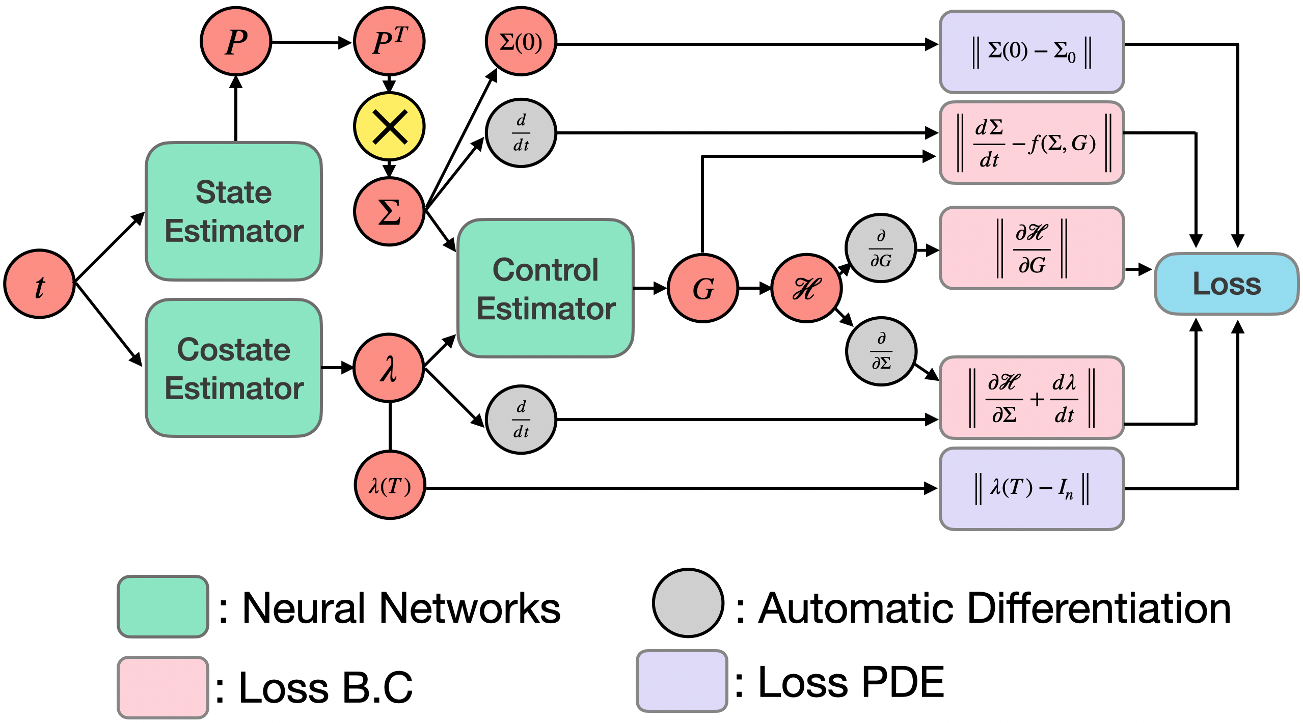
Figure 1: Our PMP-Net architecture for learning optimal linear filter. The state estimator, the costate estimator, and the control estimator are neural networks. We engineer the state estimator to output an intermediate matrix $P$ and estimates $\Sigma$ as $\Sigma=PP^{T}$ to ensure its symmetry and positive semi-definiteness. We compute the Hamiltonian $\mathcal{H}$, relevant derivatives, and residual of differential equations in PMP. The total loss function consists of loss from residuals and loss from boundary conditions. Since all loss terms are calculated based on predictions, no labeled data is needed for training

3.3 Results

For our experiment, we set

$$A\!=\!\begin{bmatrix}\bm{0}&\bm{I}_{2}\\ \bm{0}&\bm{0}\end{bmatrix}\!\in\!\mathbb{R}^{4\times 4},B=\begin{bmatrix}\bm{0}\\ \bm{I}_{2}\end{bmatrix}\!\in\!\mathbb{R}^{4\times 2},C=\bm{I}_{4},Q=0.5\bm{I}_{2},R=\!\begin{bmatrix}4.0&1.5&0&0\\ 1.5&4.0&0&0\\ 0&0&2.0&1.0\\ 0&0&1.0&2.0\end{bmatrix}\!,T=5.0$$

This dynamics system models a kinematics system where the state $x$ corresponds to position and velocity and the control $u$ corresponds to the force applied to the state. With these experimental settings, Kalman filtering reaches a steady state where $\Sigma^{\star}$ converges (hence, the Kalman gain converges to $G^{\star}_{\infty}$). We compare our method against traditional supervised learning method (baseline) trained with 50 points of ground truth control $u^{\star}$ sampled from the time interval $[0\,,\,2.0]$, covering the transient phase of the Kalman filter before it reaches steady-state.

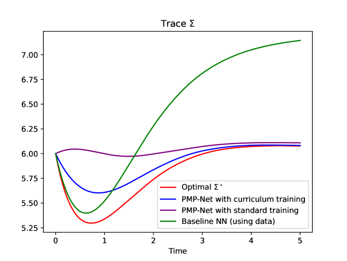
(a) Trace $\Sigma$

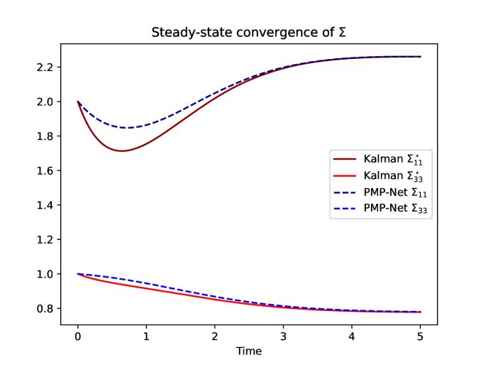
(b) Steady state convergence of $\Sigma$

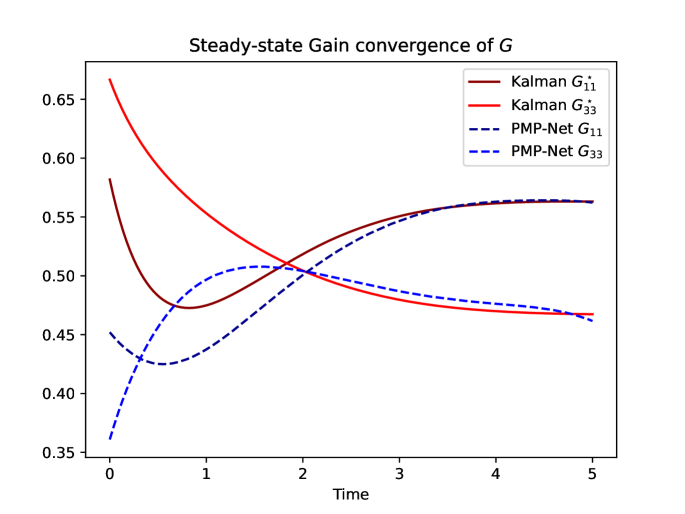
(c) Steady state convergence of $G$

Figure 2: Designing optimal linear filter with PMP-net. PMP-net has shown to replicate Kalman filter, especially deriving the optimal steady-state Kalman gain $G^{\star}_{\infty}$. While baseline NN performs well in the time interval where ground truth is available, it fails to learn the optimal steady-state Kalman gain $G^{\star}_{\infty}$, resulting in diverging error.

We evaluate and compare the trace of $\Sigma$ generated by PMP-net, the baseline method and the optimal Kalman gain. Since the objective is to minimize the trace of $\Sigma$ at the terminal time $T$, we focus primarily on the final value $\textrm{tr}(\Sigma(T))$. Figure 2(a) shows that the estimated control by PMP-net has created a trajectory with the same performance measure as the optimal Kalman gain, while the baseline diverges. Figure 2(b) and 2(c) further show that PMP-Net generates a trajectory of $(\Sigma,G)$ that converges to the optimal values. Note that there is a discrepancy between PMP-net’s control output $G$ and the Kalman gain $G^{\star}$ during the transient phase. However, this discrepancy does not affect the overall performance since PMP-net’s control $G$ converges at the optimal steady-state value $G^{\star}_{\infty}$. In practice, the steady-state $G^{\star}_{\infty}$ is often pre-computed and used instead of $G^{\star}(t)$ for efficiency.

In addition, we also investigated the effect of using curriculum training. As shown in Fig 2(a), using curriculum training results in a trajectory with smaller trace of error covariance throughout the interval of interest, especially during the transient phase. We leave further problem of optimizing $G$ during the transient phase to future work.

4 Learning optimal control for a Minimum Time problem

In this section, we seek an optimal control strategy that drives a state from an arbitrary initial position to a specified terminal position in the shortest possible time. In practice, the control is subject to constraints, such as maximum output levels. The optimal control strategy for the minimum time problem is commonly known as “bang-bang” control. Examples of bang-bang control applications include guiding a rocket to the moon in the shortest time possible while adhering to acceleration constraints (Athans & Falb, 1996); maintaining desired temperatures industrial furnaces (Burns et al., 1991); decision-making in stock options, where control switches between buying and selling based on market conditions (Kamien & Schwartz, 1991).

4.1 Minimum time problem

We illustrate the PMP-net with the following problem. Consider the kinematics system

$$\begin{bmatrix}\dot{x}_{1}(t)\\ \dot{x}_{2}(t)\end{bmatrix}=\begin{bmatrix}0&1\\ 0&0\end{bmatrix}\begin{bmatrix}x_{1}(t)\\ x_{2}(t)\end{bmatrix}+\begin{bmatrix}0\\ 1\end{bmatrix}u$$

where $x_{1},x_{2},u$ correspond to the position, velocity and acceleration. The goal is to drive the system from the initial state $(x_{1}(0),x_{2}(0))=(p_{0},v_{0})$ to a final destination $(p_{f},v_{f})$ where $x(t)\in\mathbb{R}^{n}$ is the state at time $t$, $u(t)\in\mathbb{R}^{m}$ is the control at time $t$, $A\in\mathbb{R}^{n\times n}$ is the state transition matrix and $B\in\mathbb{R}^{n\times m}$ is the input matrix. We are interested in finding the optimal control $\left\{u^{\star}(t),t\in[0\,,\,t^{\star}]\right\}$ that drives the state from $x_{0}$ to $x_{f}$ in a minimum time $t^{\star}_{f}$. The performance measure can be written as

$$J(x,u)=\displaystyle\int\limits_{0}^{t_{f}}1dt$$ (10)

where $t_{f}$ is the time in which the sequence $(x,u)$ reaches the terminal state. Note that here $t_{f}$ is a function of $(x,u)$ since the time to reach the target state depends on the state and control. In practice, the control components may be constrained by requirements such as a maximum acceleration or maximum thrust

$$|u_{i}(t)|\leq 1,\quad i\in[1,m]\quad t\in[t_{0},t_{f}]$$ (11)

where $u_{i}$ is the $i$th component of $u$. Pontryagin’s maximum principle gives us the necessary conditions at the optimal solution $(x^{\star},u^{\star},\lambda^{\star})$ for equation 12.

$$\begin{split}\begin{bmatrix}\dot{x}_{1}^{\star}\\ \dot{x}_{2}^{\star}\end{bmatrix}&=\begin{bmatrix}x_{1}^{\star}\\ 0\end{bmatrix}+\begin{bmatrix}0\\ u^{\star}\end{bmatrix}\\ \dot{\lambda^{\star}}&=\begin{bmatrix}0\\ -\lambda_{1}^{\star}\end{bmatrix}\\ u^{\star}&=\operatorname*{arg\,min}_{u}1+\lambda^{\star}_{1}x^{\star}_{2}+\lambda_{2}^{\star}u\\ 1+\lambda_{2}(t^{\star}_{f})u(t^{\star}_{f})&=0\\ x(t^{\star}_{f})&=\bm{0}\end{split}$$ (12)

4.2 Learning bang-bang control with PMP-Net

Architecture: Our PMP-Net for the minimum time problem is depicted in Figure 3. This design is inspired by classical feedback control, where the control variable $u$ is a function of both the state and the costate. In our approach, the state estimator, costate estimator, and control estimator are modeled by 6-layer feedforward networks. It is important to note that all equations and functions in equation 12 are only valid for $t\in\left[0,t^{\star}_{f}\right]$. However, since the final time $t^{\star}_{f}$ is unknown, we design our architecture to extend the applicability of equation 12 beyond time $t^{\star}_{f}$. To achieve this, we multiply the output of the control estimator by $1_{x\neq x_{f}}$, which simulates a controller that sets the control to zero once the state reaches the target destination. Because the indicator function is not differentiable, we approximate it using a scaled sigmoid function $\sigma(L\|x-x_{f}\|)$.

Lastly, instead of defining the terminal time to be the time the state reaches the target, we introduce an additional intrinsic parameter $t_{f}$ subject to the constraint $x(t_{f})=x_{f}$. This difference is subtle, yet it allows PMP-Net to learn $t_{f}$ during backpropagation.

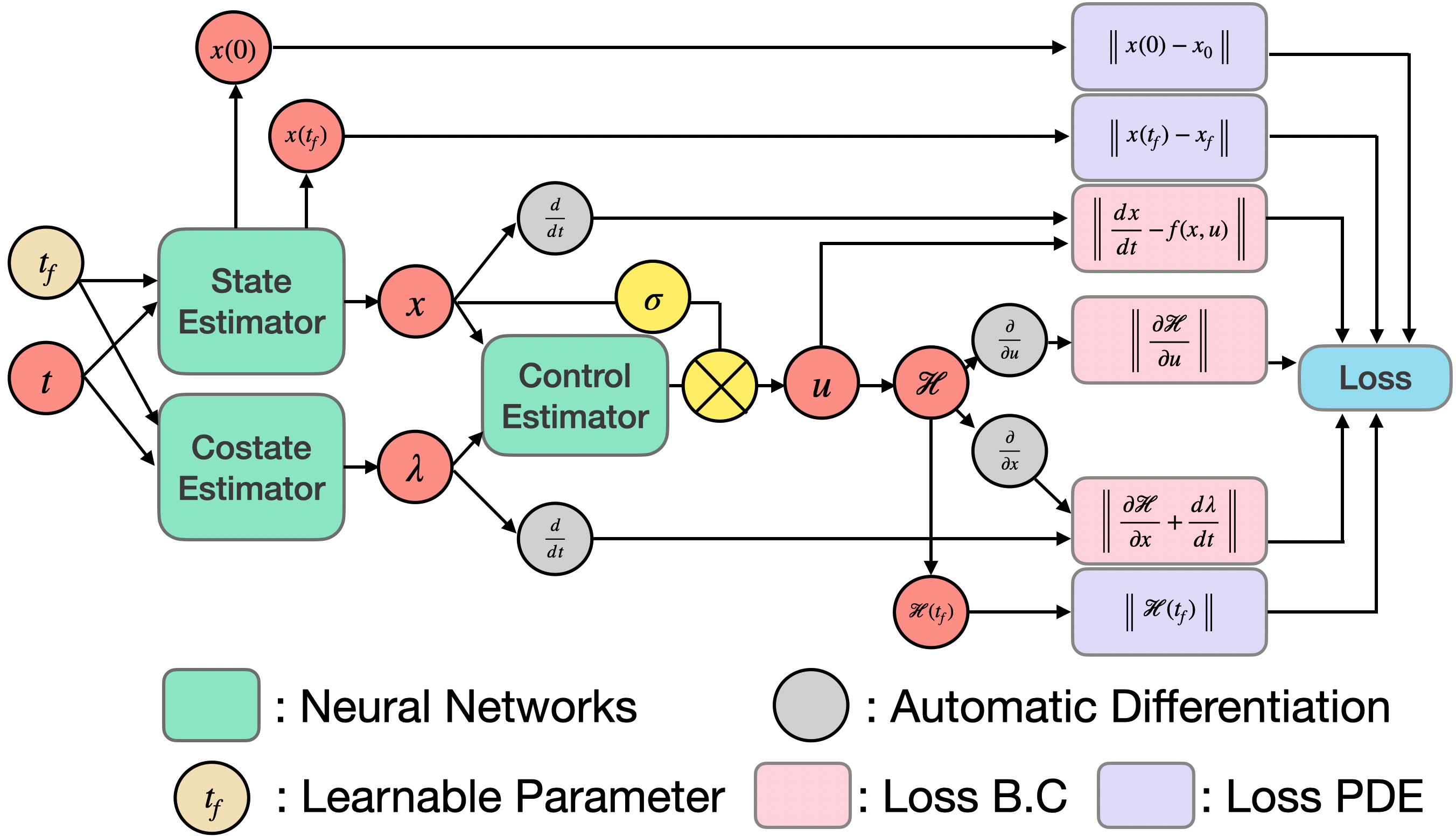
Figure 3: Our PMP-net architecture for the minimum time problem. We engineer PMP-net as follows: 1) we multiply the control estimator’s output by a scaled sigmoid of the estimated state to deactivate control once the state reaches the target, and 2) we introduce a learnable intrinsic parameter, $t_{f}$, which estimates the minimum time. These features ensure the validity of PMP beyond $t^{\star}_{f}$, enabling us to learn both bang-bang control and $t_{f}$without prior knowledge of $t^{\star}_{f}$.

Training: We propose a new paradigm for training PMP-Net for the minimum-time problems. First, we set a time $T$ that is sufficiently larger than $t^{\star}_{f}$. Firstly, we pretrain the costate estimator such that the costate estimator is not a zero function (see Appendix C). This can be achieved by training the costate estimator to output $a$ at time $0$ and $b$ at time $T$, where $a,b$ are heuristic non-zero values. Secondly, equation 12 suggests that the optimal control $u^{\star}$ as a function of $(x^{\star},\lambda^{\star})$ can be learned without knowing $(x^{\star},\lambda^{\star})$. Therefore, we can generate a random $(x,\lambda)$ and train the control estimator to minimize $\mathcal{H}(x,\lambda,u)$. Note that we freeze the state and costate estimator while training the control estimator since $u^{\star}=\operatorname*{arg\,min}_{u}\mathcal{H}(x,\lambda,u)$. We train PMP-net by uniformly sampling 5000 points are uniformly sampled from time $[0,T]$. We also compute gradient of the loss function with respect to variable $t_{f}$, allowing it to be optimized during backpropagation. We train PMP-net using stochastic gradient descent with the initial learning rate $8\times 10^{-4}$.

Evaluation: Similar to the experiment in Section 3.2, we generate the control estimate from PMP-net and use a fourth-order Runge-Kutta integrator to estimate the state trajectory. For the baseline, we employ the optimal (bang-bang) control and integrate it with the fourth-order Runge-Kutta method. During prediction, we consider the state to have reached the target if the Euclidean distance between them is less than $\epsilon=0.05$.

4.3 Results

For our experiment, we set $x_{0}=\begin{bmatrix}1\\ 0\end{bmatrix},x_{f}=\begin{bmatrix}0\\ 0\end{bmatrix}$, $T=3.0$. The optimal control is to apply the acceleration $-1$ from time $[0,1]$ and acceleration $+1$ from time $]1,2]$ that will drive the state from the initial state $x_{0}$ to the target state $x_{f}$ in minimum time $t^{\star}_{f}=2$ seconds. The control switches from $-1$ to $+1$ at the switching time at $t=1$ where $\lambda^{\star}_{2}(t)=0$ as shown in Fig 4(b)

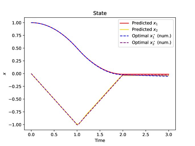
(a) Estimated state $x$

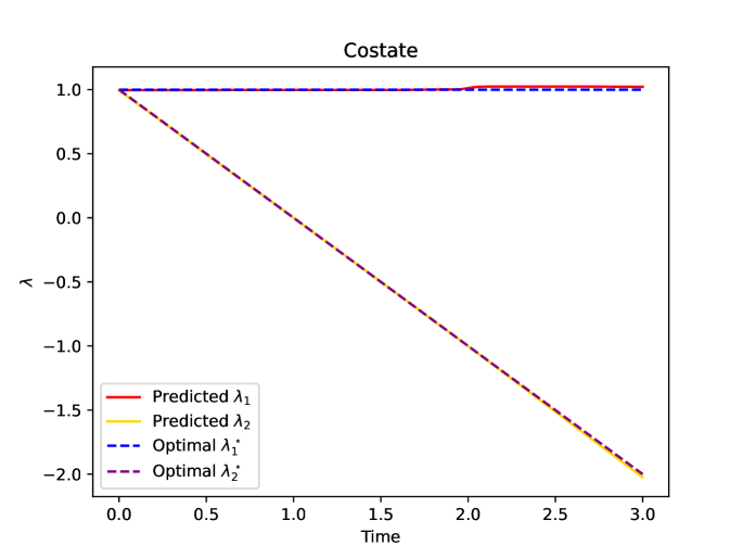
(b) Estimated costate $\lambda$

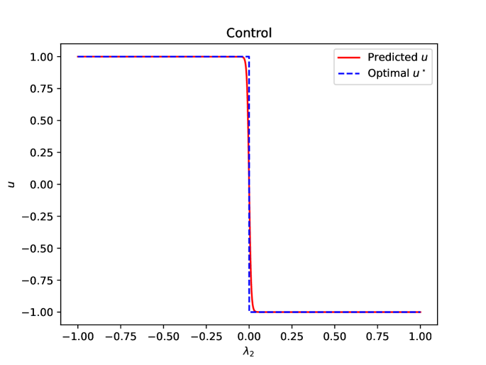
(c) Estimated control as a function of $\lambda_{2}$

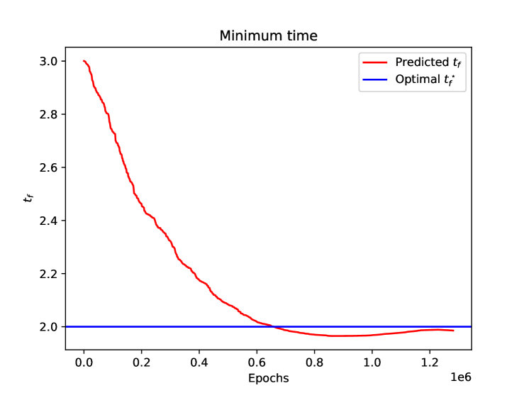
(d) Estimated $t_{f}$ learned by our PMP-net

Figure 4: Learning optimal control for minimum time problem with PMP-net. PMP-net estimates the trajectory of the state, the costate and the control over the time interval of interest that matches the optimal trajectory. Most importantly, PMP-net learns the bang-bang behavior where control $u$ is a negative sign function of $\lambda_{2}$ and correctly learns the minimum time $t^{\star}_{f}$.

Figure 4(a) and 4(b) show that the generated trajectory of state and costate matches the optimal solution. Figure 4(c) shows that PMP-net learns a control strategy that exhibits “bang-bang” behavior, switching from $+1$ to $-1$ when $\lambda_{2}$ changes sign. Since standard neural networks inherently produce continuous functions, there is a small discrepancy between the predicted control and the theoretical bang-bang control, as shown in Fig 4(c). This limitation may, in fact, better reflect real-world scenarios, as the control cannot switch instantaneously between two extremes. While reducing this discrepancy is possible by using a larger control estimator and more computational resources to compute gradients of higher magnitude, such optimization is beyond the scope of this work. Figure 4(d) has demonstrates that the trainable variable $t_{f}$ in PMP-Net successfully converges to the true value of $t^{\star}_{f}=2$. This key result highlights PMP-net’s ability to learn when the terminal time is unknown.

(a) Effect of pretraining the costate estimator

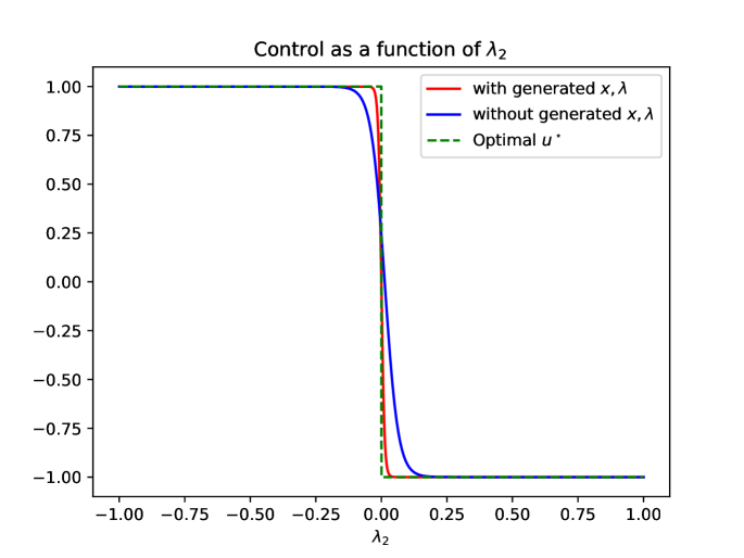
(b) Effect of using additional $x,\lambda$ to train the control estimator

Figure 5: Ablation study. We investigate the effect of pretraining the costate estimator and the effect of using additional $x,\lambda$ to train the control estimator. Fig 5(a)): PMP-net fails to train when the costate estimator is not pretrained and is initialized close to zero. Fig 5(b)): Generating additional $x,\lambda$ data to train the control estimator reduces the discrepancy between the learned control function and the optimal bang-bang solution.

We also conducted an ablation study to examine the impact of our training methods. Fig 5(a) demonstrates that when the costate estimator is initialized near the zero function, PMP-Net struggles to learn effectively, resulting in loss divergence. Moreover, we investigated the effect of adding the generated $x$ and $\lambda$ to train the control estimator. Fig 5(b) shows that the output control by the control estimator trained without using additional data does not switch at $\lambda_{2}=0$ and its rate of switching between two extremes is slower than that of the control estimator trained using additional data $x,\lambda$.

5 Related Work

Physics priors for neural network: Numerous prior works have aimed to integrate physics-based priors into neural networks for supervised learning tasks. Physics-informed Neural Networks learn supervised learning tasks while respecting any given laws of physics described by general nonlinear partial differential equations Raissi et al. (2019); Lu et al. (2021a). Hamiltonian Neural Networks (Greydanus et al., 2019) and Lagrangian Neural Networks (Lutter et al., 2019; Cranmer et al., 2020) apply physics laws and parameterize and learn Hamiltonian and Lagrangian that match observations of the systems. All of these approaches use labeled data to learn physical parameters of the dynamics system. Our approach, in contrast, does not require any labeled data to learn the optimal control function.

Learning optimal control using neural networks: Böttcher et al. (2022) enforces the dynamics constraint in neural networks using neural ODEs (Chen et al., 2018) to learn optimal control. However, this ODE-based approach does not take advantage of other optimality conditions in PMP. ODE-based methods solve the forward problem by integrating the state up to the terminal time, calculating and minimizing the loss function, but they are not applicable when the terminal time $t^{\star}_{f}$ is unknown and needs to be optimized, or when the terminal state is specified. In contrast, our work leverages the calculus of variations and PMP, enabling us to account for variations in both terminal time and terminal state, and simultaneously learn the optimal control and minimum time under these conditions.

6 Conclusion

We present a novel paradigm that integrates Pontryagin’s maximum principle into neural networks for learning the solutions to functional optimization problems arising in many engineering and technology and scientific problems. Our PMP-Net is unsupervised, generalizable and can be applied to any optimal control problem where Pontryagin’s maximum principle is applicable. We illustrate the PMP-net strategy with two classical problems of great applied significance and show that it successfully recovers the Kalman filter and bang-bang control. By leveraging the Calculus of Variations, we can analyze variations in terminal time, and PMP-Net successfully optimizes this variable in the minimum time problem—something forward methods like ODE-based approaches cannot achieve. Although these solutions have been derived analytically in the past, our work paves the way for applying PMP-based neural networks to more complex, higher-dimensional, and analytically intractable control problems.

Appendix A Calculus of variation and Pontryagin’s maximum principle

Suppose we want to find the control $u^{\star}$ that causes the system

$$\dot{x}=f(x,u)$$ (13)

to follow an admissible trajectory $x^{\star}$ that minimizes the performance measure

$$J(x,u)=q_{T}(x(t_{f}),t_{f})+\int_{0}^{t_{f}}g(x(t),u(t),t)dt$$

Assuming that $q_{T}$ is twice differentiable,

$$J(x,u) =q_{T}(x(0),0)+\int_{0}^{t_{f}}\frac{dq_{T}}{dt}(x,t)+g(x(t),u(t),t)dt$$

We introduce the Lagrange multipliers $\lambda$, also known as costates. The primary function of $\lambda$ is to enable us to make perturbations $(\delta x,\delta u)$ to an admissible trajectory $(x,u)$ while ensuring the dynamics constraints in equation 13 remain satisfied. Suppose we have an admissible trajectory $(x,u,\lambda)$ such that reaches the terminal state $x_{f}$ at time $t_{f}$, the lagrangian $\mathcal{L}$ is defined as

$$\mathcal{L}(x,u,\lambda,x_{f},t_{f}) =q_{T}(x_{0},0)+\displaystyle\int\limits_{0}^{t_{f}}\frac{dq_{T}}{dt}(x,t)+g(x,u)+\lambda^{T}(f(x,u)-\dot{x})dt$$

$$=q_{T}(x_{0},0)+\displaystyle\int\limits_{0}^{t_{f}}\frac{dq_{T}}{dt}(x(t),t)+g(x,u)+\lambda^{T}f(x,u)-\lambda^{T}\dot{x})dt$$

$$=q_{T}(x_{0},0)+\displaystyle\int\limits_{0}^{t_{f}}\frac{dq_{T}}{dt}(x(t),t)+\mathcal{H}(x,u,\lambda,t)-\lambda^{T}\dot{x})dt$$

where the Hamiltonian $\mathcal{H}=g(x,u)+\lambda^{T}f(x,u)$. The calculus of variations studies how making a small pertubation to $(x,u,\lambda)$ changes the performance. Suppose the new trajectory $(x+\delta x,u+\delta u,\lambda+\delta\lambda)$ reaches new terminal state $(x_{f}+\delta x_{f},t_{f}+\delta t_{f})$. The change in performance is

$$\Delta\mathcal{L} =\mathcal{L}(x+\delta x,u+\delta u,\lambda+\delta\lambda,x_{f}+\delta x_{f},t_{f}+\delta t_{f})-\mathcal{L}(x,u,\lambda,x_{f},t_{f})$$

$$=\displaystyle\int\limits_{0}^{t_{f}}\frac{\partial}{\partial x}\frac{dq_{T}}{dt}(x,t)\delta x+\frac{\partial\mathcal{H}}{\partial x}\delta x+\frac{\partial\mathcal{H}}{\partial u}\delta u+\left(\frac{\partial\mathcal{H}}{\partial\lambda}-\dot{x}\right)^{T}\delta\lambda-\lambda^{T}\delta xdt$$

$$\quad+\left[\frac{dq_{T}}{dt}(x(t_{f}),t_{f})+\mathcal{H}(x,u,\lambda,t_{f})-\lambda(t_{f})^{T}\dot{x}(t_{f}))\right]\delta t_{f}+o(\|\delta x\|,\|\delta u\|,\|\delta\lambda\|,\|\delta t_{f}\|)dt$$

$$=\displaystyle\int\limits_{0}^{t_{f}}\frac{\partial^{2}q_{T}}{\partial x^{2}}\dot{x}\delta x+\frac{\partial^{2}q}{\partial x\partial t}\delta x+\frac{\partial q}{\partial x}\dot{\delta x}-\lambda^{T}\dot{\delta x}+\frac{\partial\mathcal{H}}{\partial x}\delta x+\frac{\partial\mathcal{H}}{\partial u}\delta u+\left[f(x,u)-\dot{x}\right]^{T}\delta\lambda dt$$

$$\quad+\left[\frac{dq_{T}}{dt}(x(t_{f}),t_{f})+\mathcal{H}(x,u,\lambda,t_{f})-\lambda(t_{f})^{T}\dot{x}(t_{f}))\right]\delta t_{f}+o(\|\delta x\|,\|\delta u\|,\|\delta\lambda\|,\|\delta t_{f}\|)dt$$

$$=\displaystyle\left[\frac{\partial q_{T}}{\partial x}\Big{|}_{t_{f}}-\lambda(t_{f})^{T}\right]\delta x(t_{f})+\int\limits_{0}^{t_{f}}\left[\dot{\lambda}+\frac{\partial\mathcal{H}}{\partial x}\right]\delta x+\frac{\partial\mathcal{H}}{\partial u}\delta u+\left[f(x,u)-\dot{x}\right]^{T}\delta\lambda dt$$

$$\quad+\left[\frac{\partial q_{T}}{\partial x}\Big{|}_{t_{f}}\dot{x}(t_{f})+\frac{\partial q_{T}}{\partial t}\Big{|}_{t_{f}}+\mathcal{H}(x,u,\lambda,t_{f})-\lambda(t_{f})^{T}\dot{x}(t_{f}))\right]\delta t_{f}+o(\|\delta x\|,\|\delta u\|,\|\delta\lambda\|,\|\delta t_{f}\|)dt$$

$$=\left[\frac{\partial q_{T}}{\partial x}\Big{|}_{t_{f}}-\lambda(t_{f})^{T}\right]\delta x_{f}+\int\limits_{0}^{t_{f}}\left[\dot{\lambda}+\frac{\partial\mathcal{H}}{\partial x}\right]\delta x+\frac{\partial\mathcal{H}}{\partial u}\delta u+\left[f(x,u)-\dot{x}\right]^{T}\delta\lambda dt$$

$$\quad+\left[\frac{\partial q_{T}}{\partial t}\Big{|}_{t_{f}}+\mathcal{H}(x,u,\lambda,t_{f})\right]\delta t_{f}+o(\|\delta x\|,\|\delta u\|,\|\delta\lambda\|,\|\delta t_{f}\|)dt$$

The fundamental theorem of calculus of variation states that if $(x^{\star},u^{\star})$ is extrema, then the variations $\delta J$ (linear terms of $\delta x,\delta u,\delta x_{f},\delta t_{f}$) must be zero. Since $\lambda$ can be chosen arbitrarily, we choose $\lambda^{\star}$ such that the linear terms of $\delta x$ is $0$, i.e.

$$\dot{\lambda}^{\star}+\frac{\partial\mathcal{H}}{\partial x}\Big{|}_{\star}=0$$ (14)

Since the $(x^{\star},u^{\star})$ must satisfy the constraint in equation 13,

$$f(x^{\star},u^{\star})-\dot{x}^{\star}=0$$ (15)

The remaining variation $\delta u$ is independent, so its coefficient must be zero; thus,

$$\frac{\partial\mathcal{H}}{\partial u}\Big{|}_{\star}=0$$ (16)

The rest of variations are therefore $0$, i.e.,

$$\left[\frac{\partial q_{T}}{\partial x}\Big{|}_{\star,t^{\star}_{f}}-\lambda(t^{\star}_{f})^{T}\right]\delta x_{f}+\left[\frac{\partial q_{T}}{\partial t}\Big{|}_{\star,t^{\star}_{f}}+\mathcal{H}(x^{\star},u^{\star},\lambda^{\star},t^{\star}_{f})\right]\delta t_{f}=0$$

If the terminal state is fixed and terminal time is free, $\delta x_{f}=0$ and $\delta t_{f}$ can be arbitrarily. The coefficients of $\delta t_{f}$ must be $0$, i.e.,

$$\begin{split}\left[\frac{\partial q_{T}}{\partial t}\Big{|}_{\star,t^{\star}_{f}}+\mathcal{H}(x^{\star},u^{\star},\lambda^{\star},t^{\star}_{f})\right]&=0\\ x^{\star}(t^{\star}_{f})=x_{f}\end{split}$$ (17)

If the terminal time is fixed and terminal state is free, $\delta t_{f}=0$ and $\delta x_{f}$ can be arbitrarily. The coefficients of $\delta x_{f}$ must be $0$, i.e.,

$$\begin{split}\left[\frac{\partial q_{T}}{\partial x}\Big{|}_{\star,t^{\star}_{f}}-\lambda(t^{\star}_{f})^{T}\right]=0\\ t^{\star}_{f}=t_{f}\end{split}$$ (18)

The equation 17 and equation 18 allow us to determine the optimal terminal state or optimal terminal time when they are free and to be optimized. These equations from 14 to  18 are called Pontryagin’s maximum principle.

Appendix B Kalman Filtering Derivation

The performance measure for designing optimal linear filter is

$$J(\Sigma,G) =q_{T}(\Sigma(T),T)$$

$$=\textrm{tr}(\Sigma(T))$$

Since the terminal time $t_{f}=T$ is specified and terminal state is free,  equation 18 applies. Pontryagin’s maximum principle yields

$$\dot{\Sigma}^{\star}=\Bigl{[}A-G^{\star}C\Bigr{]}\Sigma\!+\Sigma\Big{[}A\!-G^{\star}C\Big{]}^{T}\!+BQB^{T}\!+G^{\star}R{G^{\star}}^{T}$$ (19a)

$$\frac{\partial\textrm{tr}(\lambda^{\star}\dot{\Sigma}^{\star})}{\partial\Sigma}\Big{|}_{\star}+\dot{\lambda^{\star}}^{T}=0$$ (19b)

$$\frac{\partial\textrm{tr}(\lambda^{\star}\dot{\Sigma}^{\star})}{\partial G}\Big{|}_{\star}=0$$ (19c)

$$\lambda^{\star}(T)^{T}=\bm{I}_{n}$$ (19d)

$$\Sigma^{\star}(0)=\Sigma_{0}$$ (19e)

Simplifying equation 19b yields,

$$\dot{\lambda}^{\star}=-\lambda^{\star}\Bigl{[}A-G^{\star}C\Bigr{]}-\Bigl{[}A-G^{\star}C\Bigr{]}^{T}\lambda^{\star}$$ (20)

From equation 19d and equation 20, we can conclude that $\lambda^{\star}$ is symmetric positive definite. Substitute $\dot{\Sigma}^{\star}$ in equation 19c by R.H.S expression in equation 19a yields,

$$2\lambda^{\star}\Bigl{[}2G^{\star}R-2{\Sigma^{\star}}C^{T}\Bigr{]}=0$$ (21)

Since $\lambda^{\star}$ is invertible,

$$G^{\star}={\Sigma^{\star}}C^{T}R^{-1}$$ (22)

Plugging this solution $G^{\star}$ in equation 19a yields

$$\dot{\Sigma}^{\star}=A\Sigma^{\star}+\Sigma^{\star}A^{T}+BQB-\Sigma^{\star}C^{T}R^{-1}C\Sigma^{\star}$$ (23)

which is the matrix differential equation of the Riccati type. The solution $\Sigma^{\star}$ can be derived from the initial condition $\Sigma^{\star}(0)=\Sigma_{0}$ and the differential equation 23.

Appendix C Bang-bang control derivation

Since the terminal state $x_{f}$ is specified and terminal time is free,  equation 17 applies. Pontryagin’s maximum principle yields

$$\dot{x}^{\star}=\begin{bmatrix}x^{\star}_{2}\\ 0\end{bmatrix}+\begin{bmatrix}0\\ u^{\star}\end{bmatrix}$$ (24a)

$$\dot{\lambda}^{\star}=\begin{bmatrix}0\\ -\lambda_{1}^{\star}\end{bmatrix}\\$$ (24b)

$$u^{\star}=\operatorname*{arg\,min}_{u}1+\lambda^{\star}_{1}x^{\star}_{2}+\lambda^{\star}_{2}u$$ (24c)

$$1+\lambda_{1}^{\star}(t^{\star}_{f})x^{\star}_{2}(t^{\star}_{f})+\lambda^{\star}_{2}(t^{\star}_{f})u^{\star}(t^{\star}_{f})=0$$ (24d)

$$\begin{bmatrix}x^{\star}_{1}(0)\\ x^{\star}_{2}(0)\end{bmatrix}=\begin{bmatrix}x_{0}\\ v_{0}\end{bmatrix}$$ (24e)

$$\begin{bmatrix}x^{\star}_{1}(t^{\star}_{f})\\ x^{\star}_{2}(t^{\star}_{f})\end{bmatrix}=\begin{bmatrix}0\\ 0\end{bmatrix}$$ (24f)

The equation 24c yield

$$\forall u,1+\lambda_{1}^{\star}x_{2}+\lambda_{2}^{\star}u^{\star} \leq 1+\lambda_{1}^{\star}x_{2}+\lambda_{2}^{\star}u$$

$$u^{\star}=\begin{cases}-\textrm{sign}(\lambda_{2})&\textrm{if $\lambda_{2}^{\star}\neq 0$}\\ \quad\textrm{indeterminate}&\textrm{if $\lambda_{2}^{\star}=0$}\end{cases}$$

Assuming that $\lambda^{\star}_{2}$ is not a zero function, the equation 24b yields

$$\begin{split}\lambda^{\star}_{1}(t)&=c_{1}\\ \lambda^{\star}_{2}(t)&=-c_{1}t+c_{2}\\ \end{split}$$ (25)

where $c_{1},c_{2}$ are constants to be determined. We see from equation 25 that $\lambda_{2}$ changes sign at most once. There are two possible cases:

1. $\lambda^{\star}_{2}$ sign remains constant in $[0,t^{\star}_{f}]$

2. $\lambda^{\star}_{2}$ changes sign in $[0,t^{\star}_{f}]$

For case 1, we have the general form of

$$\begin{split}x_{2}(t)&=v_{0}+at\quad\qquad\textrm{for $t\in[0,t^{\star}_{f}]$}\\ x_{1}(t)&=p_{0}+v_{0}t+\displaystyle\frac{1}{2}at^{2}\;\ \quad\textrm{for $t\in[0,t^{\star}_{f}]$}\end{split}$$ (26)

For case 2, we have the general form of $x$

$$\begin{split}x_{2}(t)&=\begin{cases}v_{0}+at&\quad\textrm{if }{t\leq t_{m}}\\ v_{0}+at_{m}-a(t-t_{m})&\quad\textrm{if }{t^{\star}_{f}\geq t\geq t_{m}}\end{cases}\\ x_{1}(t)&=\begin{cases}p_{0}+v_{0}t+\displaystyle\frac{1}{2}at^{2}&\quad\textrm{if }{t\leq t_{m}}\\ x_{0}+v_{0}t+3att_{m}-2at_{m}^{2}-\displaystyle\frac{1}{2}at^{2}&\quad\textrm{if }{t\geq t_{m}}\\ \end{cases}\end{split}$$ (27)

where $a=\pm 1$ and $t_{m}$ is the time where $\lambda^{\star}_{2}$ switches sign. To determine which case corresponds to the system, we validate with the boundary condition. Suppose we try with the general expression in equation 27 and substitute in boundary conditions in equation 24:

$$\begin{split}-c_{1}t_{m}+c_{2}&=0\quad\quad\textrm{( From the condition $\lambda^{\star}_{2}(t_{m})=0$)}\\ a&=\pm 1\\ v_{0}+at_{m}-a(t_{f}-t_{m})&=0\quad\quad\textrm{( From equation~{}\ref{eq:bangbang_end}})\\ p_{0}+v_{0}t+3at_{f}t_{m}-2at_{m}^{2}-\displaystyle\frac{1}{2}at_{f}^{2}&=0\quad\quad\textrm{( From equation~{}\ref{eq:bangbang_end}})\\ 1-a(c_{1}t_{f}+c_{2})&=0\quad\quad\textrm{( From equation~{}\ref{eq:bangbang_bc}})\end{split}$$ (28)

Specific example: $x_{0}=1,v_{0}=0$.

Solving equation 28 yields

$$\begin{split}t_{f}&=2t_{m}\\ 1&=-at_{m}^{2}\\ a&=-1\\ t_{m}&=1\\ c_{1}&=1\\ c_{2}&=1\end{split}$$ (29)

which means the system with initial state condition $(1,0)$ falls the second case. If we substitute the general expression equation 26 instead, there would be no solutions satisfying equation 28.

Remarks: This derivation of bang-bang solution is based on assumption that $\lambda$ is not a zero function.

References

- Athans & Falb (1996) J. M. Athans and P. L. Falb. Optimal Control: An Introduction to the Theory and Its Applications. McGraw- Hill, New York, 1996.
- Athans & Tse (1967) M. Athans and E. Tse. A direct derivation of the optimal linear filter using the maximum principle. IEEE Transactions on Automatic Control, 12(6):690–698, 1967. doi: 10.1109/TAC.1967.1098732.
- Auger et al. (2013) François Auger, Mickael Hilairet, Josep M. Guerrero, Eric Monmasson, Teresa Orlowska-Kowalska, and Seiichiro Katsura. Industrial applications of the kalman filter: A review. IEEE Transactions on Industrial Electronics, 60(12):5458–5471, 2013. doi: 10.1109/TIE.2012.2236994.
- Baydin et al. (2017) Atılım Günes Baydin, Barak A. Pearlmutter, Alexey Andreyevich Radul, and Jeffrey Mark Siskind. Automatic differentiation in machine learning: a survey. J. Mach. Learn. Res., 18(1):5595–5637, jan 2017. ISSN 1532-4435.
- Ben-Yishai et al. (1995) Rani Ben-Yishai, Ruth Lev Bar-Or, , H Sompolinskyt, and Pierre Hohenberg. Theory of orientation tuning in visual cortex. Proceedings of the National Academy of Sciences of the United States of America, 92:3844 – 3848, 1995. URL https://api.semanticscholar.org/CorpusID:1338584.
- Burns et al. (1991) Patrick J. Burns, Kyuil Han, and C.Byron Winn. Dynamic effects of bang-bang control on the thermal performance of walls of various constructions. Solar Energy, 46(3):129–138, 1991. ISSN 0038-092X. doi: https://doi.org/10.1016/0038-092X(91)90086-C. URL https://www.sciencedirect.com/science/article/pii/0038092X9190086C.
- Böttcher et al. (2022) Lucas Böttcher, Nino Antulov-Fantulin, and Thomas Asikis. Ai pontryagin or how artificial neural networks learn to control dynamical systems. Nature Communications, 13, 01 2022. doi: 10.1038/s41467-021-27590-0.
- Chen et al. (2018) Ricky T. Q. Chen, Yulia Rubanova, Jesse Bettencourt, and David K Duvenaud. Neural ordinary differential equations. In S. Bengio, H. Wallach, H. Larochelle, K. Grauman, N. Cesa-Bianchi, and R. Garnett (eds.), Advances in Neural Information Processing Systems, volume 31. Curran Associates, Inc., 2018. URL https://proceedings.neurips.cc/paper_files/paper/2018/file/69386f6bb1dfed68692a24c8686939b9-Paper.pdf.
- Cranmer et al. (2020) Miles Cranmer, Sam Greydanus, Stephan Hoyer, Peter Battaglia, David Spergel, and Shirley Ho. Lagrangian neural networks, 2020. URL https://arxiv.org/abs/2003.04630.
- Cybenko (1989) George V. Cybenko. Approximation by superpositions of a sigmoidal function. Mathematics of Control, Signals and Systems, 2:303–314, 1989. URL https://api.semanticscholar.org/CorpusID:3958369.
- Glorot & Bengio (2010) Xavier Glorot and Yoshua Bengio. Understanding the difficulty of training deep feedforward neural networks. In International Conference on Artificial Intelligence and Statistics, 2010. URL https://api.semanticscholar.org/CorpusID:5575601.
- Greydanus et al. (2019) Samuel Greydanus, Misko Dzamba, and Jason Yosinski. Hamiltonian neural networks. In H. Wallach, H. Larochelle, A. Beygelzimer, F. d'Alché-Buc, E. Fox, and R. Garnett (eds.), Advances in Neural Information Processing Systems, volume 32. Curran Associates, Inc., 2019. URL https://proceedings.neurips.cc/paper_files/paper/2019/file/26cd8ecadce0d4efd6cc8a8725cbd1f8-Paper.pdf.
- Kalman & Bucy (1961) Rudolf E. Kalman and Richard S. Bucy. New results in linear filtering and prediction theory. Journal of Basic Engineering, 83:95–108, 1961. URL https://api.semanticscholar.org/CorpusID:8141345.
- Kamien & Schwartz (1991) Morton I. Kamien and Nancy L. Schwartz. Dynamic Optimization: The Calculus of Variations and Optimal Control in Economics and Management. North-Holland, 1991.
- Krishnapriyan et al. (2021) Aditi S. Krishnapriyan, Amir Gholami, Shandian Zhe, Robert Kirby, and Michael W Mahoney. Characterizing possible failure modes in physics-informed neural networks. Advances in Neural Information Processing Systems, 34, 2021.
- Leonard et al. (1985) Leonard, A. McGee, Stanley, and Frank R. Schmidt. Discovery of the kalman filter as a practical tool for aerospace and industry. 1985. URL https://api.semanticscholar.org/CorpusID:106584647.
- Lu et al. (2021a) Lu Lu, Xuhui Meng, Zhiping Mao, and George Em Karniadakis. DeepXDE: A deep learning library for solving differential equations. SIAM Review, 63(1):208–228, 2021a. doi: 10.1137/19M1274067.
- Lu et al. (2021b) Lu Lu, Raphaël Pestourie, Wenjie Yao, Zhicheng Wang, Francesc Verdugo, and Steven G. Johnson. Physics-informed neural networks with hard constraints for inverse design. SIAM Journal on Scientific Computing, 43(6):B1105–B1132, 2021b. doi: 10.1137/21M1397908. URL https://doi.org/10.1137/21M1397908.
- Lutter et al. (2019) Michael Lutter, Christian Ritter, and Jan Peters. Deep lagrangian networks: Using physics as model prior for deep learning. In International Conference on Learning Representations, 2019. URL https://openreview.net/forum?id=BklHpjCqKm.
- Raissi et al. (2019) M. Raissi, P. Perdikaris, and G.E. Karniadakis. Physics-informed neural networks: A deep learning framework for solving forward and inverse problems involving nonlinear partial differential equations. Journal of Computational Physics, 378:686–707, 2019. ISSN 0021-9991. doi: https://doi.org/10.1016/j.jcp.2018.10.045. URL https://www.sciencedirect.com/science/article/pii/S0021999118307125.
- Runge (1895) C. Runge. Ueber die numerische auflösung von differentialgleichungen. Mathematische Annalen, 46:167–178, 1895. URL http://eudml.org/doc/157756.