Think While You Generate: Discrete Diffusion with Planned Denoising

Abstract

Discrete diffusion has achieved state-of-the-art performance, outperforming or approaching autoregressive models on standard benchmarks. In this work, we introduce Discrete Diffusion with Planned Denoising (DDPD), a novel framework that separates the generation process into two models: a planner and a denoiser. At inference time, the planner selects which positions to denoise next by identifying the most corrupted positions in need of denoising, including both initially corrupted and those requiring additional refinement. This plan-and-denoise approach enables more efficient reconstruction during generation by iteratively identifying and denoising corruptions in the optimal order. DDPD outperforms traditional denoiser-only mask diffusion methods, achieving superior results on language modeling benchmarks such as text8, OpenWebText, and token-based generation on ImageNet $256\times 256$. Notably, in language modeling, DDPD significantly reduces the performance gap between diffusion-based and autoregressive methods in terms of generative perplexity. Code is available at github.com/liusulin/DDPD.

1 Introduction

Generative modeling of discrete data has recently seen significant advances across various applications, including text generation [5], biological sequence modeling [25; 4], and image synthesis [8; 9]. Autoregressive transformer models have excelled in language modeling but are limited to sequential sampling, with performance degrading without annealing techniques such as nucleus (top-p) sampling [20]. In contrast, diffusion models offer more flexible and controllable generation, proving to be more effective for tasks that lack natural sequential orderings, such as biological sequence modeling [25; 1] and image token generation [8]. In language modeling, the performance gap between discrete diffusion and autoregressive models has further narrowed recently, thanks to improved training strategies [29; 36; 34; 13], however, a gap still remains on some tasks [36; 29].

State-of-the-art discrete diffusion methods train a denoiser (or score) model that determines the transition rate (or velocity) from the current state to predicted values. During inference, the generative process is discretized into a finite number of steps. At each step, the state values are updated based on the transition probability, which is obtained by integrating the transition rate over the timestep period.

In order to further close the performance gap with autoregressive models, we advocate for a rethinking of the standard discrete diffusion design methodology. We propose a new framework Discrete Diffusion with Planned Denoising (DDPD), that divides the generative process into two key components: a planner and a denoiser, facilitating a more adaptive and efficient sampling procedure. The process starts with a sequence of tokens initialized with random values. At each timestep, the planner model examines the sequence to identify the position most likely to be corrupted and in need of denoising. The denoiser then predicts the value for the selected position, based on the current noisy sequence. The key insight behind our plan-and-denoise approach is that the generative probability at each position can be factorized into two components: 1) the probability that a position is corrupted, and 2) the probability of denoising it according to the data distribution.

The advantages of our approach are two-fold, providing both a simplified learning process and a more effective sampling algorithm. First, by decomposing the originally complex task into two distinct sub-tasks, the task becomes easier for each neural network model. In particular, the task of planning is simpler to learn compared to denoising. In contrast, the original uniform diffusion model relies on a single neural network to perform both tasks simultaneously.

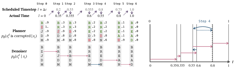
Figure 1: An example generation trajectory from $t=0$ to $1$ with a sequence of $5$ letters. At each step, the planner predicts the probability of each token being corrupted (indicated by the numbers next to the tokens). Based on these probabilities, a position is selected, and the denoiser makes its prediction. The actual time progression may not always align with the scheduled timestep, and is determined based on planner’s assessment of the noise level of the sequence. For instance, in step $2$, the denoiser makes minimal improvement and time progresses slower than scheduled. In step $4$, the denoiser made an unintended error, the time progression is effectively backward. Sampling continues until all corrupted tokens are reconstructed.

Under our framework, the mask diffusion approach achieves a comparable decomposition by using a mask token to indicate whether a position contains noise or data. However, a critical limitation of this is that once tokens are filled in, they cannot be further corrected, even if the denoiser makes errors. Furthermore, our plan-and-denoise framework enables an improved adaptive sampling scheme that leverages the planner’s predictions in two ways. Our sampling method employs finer discretization when the planner detects that the sequence is noisier than expected for the current timestep, i.e., more denoising moves are needed for the time left. Additionally, the planner can identify errors from previous steps, allowing the sampling process to adjust its time back and continue until the denoiser corrects all previously accumulated mistakes, resulting in a more robust generation. Fig. 1 provides an illustrative example of how the planner operates during inference.

Our contributions are as follows:

• We introduce Discrete Diffusion with Planning and Denoising (DDPD), a novel framework for discrete generative modeling that decomposes the generation process into planning and denoising.

• Our proposed plan-and-denoise framework introduces an adaptive sampling scheme, guided by the planner’s output, enabling continuous self-correction of errors in an optimal order. This results in improved generation by scaling the number of sampling steps.

• We derive simple and effective training objectives for the planner and denoiser models, grounded in maximizing the Evidence Lower Bound (ELBO) for discrete diffusion processes.

• In experiments on GPT-2 scale language modeling and $256\times 256$ image token generation, DDPD significantly outperforms its mask diffusion counterparts when using the same denoiser. Furthermore, we demonstrate that incorporating a planner substantially enhances generation quality, even when using a smaller or weaker denoiser model compared to baseline methods.

2 Preliminaries

We begin by introducing the problem setup and notations. Following [7; 13], we then explain the Continuous Time Markov Chain (CTMC) framework [31], which is used to define the forward and reverse processes of discrete diffusion, and how the discrete timestep version is derived from it.

Setup and Notations.  We aim to model discrete data where a sequence $x\in\{1,\cdots,S\}^{D}$ is $D$-dimensional and each element $x^{d}$ takes $S$ possible states. $x^{\backslash d}$ denotes all dimensions except $d$. For clarity in presentation, we assume $D=1$ and all results hold for $D>1$ (see Section 3.1). We use $p(x)$ to denote the probability mass function (PMF). The $\delta\left\{i,j\right\}$ is the Kronecker delta function, which is $1$ when $i=j$ and $0$ otherwise.

Continuous Time Markov Chains and Discretization.  We adopt the CTMC framework to define the discrete diffusion process. A realization of the CTMC dynamics is defined by a trajectory $x_{t}$ over time $t\in[0,1]$ that makes jumps to another state after a random waiting period known as the holding time. The transition rates and the next states are governed by the rate matrix $R_{t}\in{}^{S\times S}$ (analogous to the velocity field $\nu_{t}$ in continuous state spaces), where the off-diagonal elements, representing jumps to different states, are non-negative. For an infinitesimal timestep $\mathrm{d}t$, the probability of transitioning from $x_{t}$ to a different state $j$ is given by $R_{t}(x_{t},j)\mathrm{d}t$.

In practice, the trajectory is simulated using finite time intervals $\Delta t$. As a result, the transition probability follows a categorical distribution with the PMF [39]:

$$p_{t+\Delta t|t}(j|x_{t})=\delta\left\{x_{t},j\right\}+R_{t}(x_{t},j)\Delta t,$$ (1)

where we denote this as $\mathrm{Cat}(\delta\left\{x_{t},j\right\}+R_{t}(x_{t},j)\Delta t)$, and $R_{t}(x_{t},x_{t})\vcentcolon=-\sum_{s\neq x_{t}}R_{t}(x_{t},s)$ to ensure that the transition probabilities sum to 1.

Forward Corruption Process.  Following [7; 34; 13], which were inspired by flow matching in continuous state space [26; 27; 2], we construct the forward process by interpolating from noise $p_{0}(x_{0})=p_{\mathrm{noise}}(x_{0})$ to clean data $p_{1}(x_{1})=p_{\mathrm{data}}(x_{1})$. Common choices for the noise distribution include: (i) $p_{\mathrm{noise}}^{\mathrm{unif}}(x_{t})=\nicefrac{{1}}{{S}}$, a uniform distribution over $\{1,\cdots,S\}$; and (ii) $p_{\mathrm{noise}}^{\mathrm{mask}}(x_{t})=\delta\left\{\mathbb{M},x_{t}\right\}$, a delta PMF concentrated on an artificially introduced mask state $\mathbb{M}$. Let $\alpha_{t}$ be the noise schedule that introduces noise to the data over time $t$. For example, a linear schedule is given by $\alpha_{t}=t$. The conditional marginal $p_{t|1}(x_{t}|x_{1})$ is given in closed form:

$$p_{t|1}^{\mathrm{unif}}(x_{t}|x_{1}) =\mathrm{Cat}(\alpha_{t}\delta\left\{x_{1},x_{t}\right\}+(1-\alpha_{t})\frac{1}{S}),$$ (2)

$$p_{t|1}^{\mathrm{mask}}(x_{t}|x_{1}) =\mathrm{Cat}(\alpha_{t}\delta\left\{x_{1},x_{t}\right\}+(1-\alpha_{t})\delta\left\{\mathbb{M},x_{t}\right\}).$$ (3)

At $t=1$, the conditional marginal converges to the datapoint $x_{1}$, i.e. $\delta\left\{x_{1},x_{t}\right\}$. At $t=0$, the conditional marginal converges to the noise distribution $p_{\mathrm{noise}}(x_{t})$.

Reverse Generation Process.  Sampling from $p_{\mathrm{data}}$ is achieved by learning a generative rate matrix $R_{t}(x_{t},j)$ to reverse simulate the process from $t=0$ to $t=1$ using Eq. 1, such that we begin with samples of $p_{\mathrm{noise}}$ and end with samples of $p_{\mathrm{data}}$. The datapoint conditional reverse rate $R_{t}(x_{t},j|x_{1})$ for $j\neq x_{t}$ under the uniform or mask noise distributions is given by [7; 13]:

$$R_{t}^{\mathrm{unif}}(x_{t},j|x_{1})=\frac{\dot{\alpha_{t}}}{1-\alpha_{t}}\delta\left\{x_{1},j\right\}(1-\delta\left\{x_{1},x_{t}\right\}),\quad R_{t}^{\mathrm{mask}}(x_{t},j|x_{1})=\frac{\dot{\alpha_{t}}}{1-\alpha_{t}}{\delta\left\{x_{1},j\right\}\delta\left\{x_{t},\mathbb{M}\right\}}.$$

[7; 13] show that the rate we aim to learn for generating $p_{\mathrm{data}}$ is the expectation of the data-conditional rate, taken over the denoising distribution, i.e., $R_{t}(x_{t},j)\vcentcolon=\mathbb{E}_{p_{1|t}(x_{1}|x_{t})}\left[R_{t}(x_{t},j|x_{1})\right]$:

$$R_{t}^{\mathrm{unif}}(x_{t},j)=\frac{\dot{\alpha_{t}}}{1-\alpha_{t}}p_{1|t}\left(x_{1}=j|x_{t}\right),\quad R_{t}^{\mathrm{mask}}(x_{t},j)=\frac{\dot{\alpha_{t}}}{1-\alpha_{t}}{\delta\left\{x_{t},\mathbb{M}\right\}}p_{1|t}\left(x_{1}=j|x_{t}\right).$$ (4)

The goal is to approximate this rate using a neural network. During inference, the generative process is simulated with the learned rate by taking finite timesteps, as described in Eq. 1.

Table 1: Specific design choices employed by different discrete diffusion models.

	SDDM [39]	SEDD [29]	DFM [7] / Discrete FM [13]	MDLM [34] / MD4 [36]	Ours (‘DDPD’) Ö
Sampling (Section 3.2)
Method	Tau-leaping	Tau-leaping	Tau-leaping	Tau-leaping	Adaptive Gillespie
Time steps $t_{i}$	$\nicefrac{{i}}{{N}}$	$\nicefrac{{i}}{{N}}$	$\nicefrac{{i}}{{N}}$	$\nicefrac{{i}}{{N}}$	[t][5ex]$t_{\theta}(x_{i})+\tau_{i}$,
					$\tau_{i}\sim\mathrm{Exp}\left(\lambda_{\theta}(x_{i})\right)$     (${\dagger}$)
Noise schedule$=\nicefrac{{1}}{{4}}/\sqrt{\sigma^{2}+1}\sigma_{\text{data}}^{2}/\left(\sigma^{2}+\sigma_{\text{data}}^{2}\right)$	$\alpha_{t}$	$\alpha_{t}$	$\alpha_{t}$    (${\ddagger}$)	$\alpha_{t}$    ($*$)	$\alpha_{t}$
Generative rate parameterization (Section 3.1)
Masking$=\nicefrac{{1}}{{4}}/\sqrt{\sigma^{2}+1}\sigma_{\text{data}}^{2}/\left(\sigma^{2}+\sigma_{\text{data}}^{2}\right)$	–	[t][5ex]$\frac{\dot{\alpha_{t}}}{\alpha_{t}}\delta\left\{x_{t}^{d},M\right\}\cdot$
$s_{\theta}\left(x_{t}\right)_{x_{t}^{d}\to j}$	[t][5ex]$\nicefrac{{\dot{\alpha_{t}}\delta\left\{x_{t}^{d},M\right\}}}{{1-\alpha_{t}}}\cdot$
$p_{\theta}\left(x_{1}^{d}=j|x_{t}\right)$	[t][5ex]$\nicefrac{{\dot{\alpha_{t}}\delta\left\{x_{t}^{d},M\right\}}}{{1-\alpha_{t}}}\cdot$
$p_{\theta}\left(x_{1}^{d}=j|x_{t}\right)$	–
Uniform$=\nicefrac{{1}}{{4}}/\sqrt{\sigma^{2}+1}\sigma_{\text{data}}^{2}/\left(\sigma^{2}+\sigma_{\text{data}}^{2}\right)$$\underset{i}{\operatorname{arg\,min}}$$=\nicefrac{{1}}{{4}}/\sqrt{\sigma^{2}+1}\sigma_{\text{data}}^{2}/\left(\sigma^{2}+\sigma_{\text{data}}^{2}\right)$	[t][5ex]$\frac{\dot{\alpha_{t}}}{S\alpha_{t}}\cdot$
$\frac{p_{\theta}\left(x_{t}^{d}=j|x_{t}^{\backslash d}\right)}{p_{\theta}\left(x_{t}^{d}=x_{t}^{d}|x_{t}^{\backslash d}\right)}$	[t][5ex]$\frac{\dot{\alpha_{t}}}{S\alpha_{t}}\cdot$
$s_{\theta}\left(x_{t}\right)_{x_{t}^{d}\to j}$	[t][5ex]$\nicefrac{{\dot{\alpha_{t}}}}{{1-\alpha_{t}}}\cdot$
$p_{\theta}\left(x_{1}^{d}=j|x_{t}\right)$	–	[t][5ex]$\nicefrac{{\dot{\alpha_{t}}}}{{1-\alpha_{t}}}p_{\theta}(z_{t}^{d}=N|x_{t})\cdot$
$p_{\theta}\left(x_{1}^{d}=j|x_{t},z_{t}^{d}=N\right)$
‡ DFM assumes a linear schedule. ∗ MD4 also supports learnable schedule of $\alpha_{t}$. † $\lambda_{\theta}(x_{i})$ is the total rate of jump determined by the planner.

3 Method

3.1 Decomposing Generation into Planning and Denoising

Recent state-of-the-art discrete diffusion methods [39; 29; 7; 36; 34; 13] have converged on parameterizing the generative rate using a denoising neural network and deriving cross-entropy-based training objectives. This enables simplified and effective training, leading to better and SOTA performance in discrete generative modeling compared to earlier approaches [3; 6]. In Table 1, we summarize the commonalities and differences in the design choices across various methods.

Based on the optimal generative rate in Eq. 4, we propose a new approach to parameterizing the generative rate by dividing it into two distinct components: planning and denoising. We begin by examining how the generative rate in mask diffusion can be interpreted within our framework, followed by a derivation of the decomposition for uniform diffusion.

Mask Diffusion.  For mask diffusion, the planning part is assigning probability of $\frac{\dot{\alpha_{t}}}{1-\alpha_{t}}{\delta\left\{x_{t},\mathbb{M}\right\}}\Delta t$ for the data to be denoised with an actual value. ${\delta\left\{x_{t},\mathbb{M}\right\}}$ tells if the data is noisy ($\mathbb{M}$) or clean. $\frac{\dot{\alpha_{t}}}{1-\alpha_{t}}$ is the rate of denoising, which is determined by the remaining time according to the noise schedule. The denoiser $p_{1|t}$ assigns probabilities to the possible values to be filled in if this transition happens.

$$\textstyle R_{t}^{\mathrm{mask}}(x_{t},j)\Delta t=\underbrace{\frac{\dot{\alpha_{t}}}{1-\alpha_{t}}{\delta\left\{x_{t},\mathbb{M}\right\}}}_{\text{rate of making correction}}\Delta t\underbrace{p_{1|t}\left(x_{1}=j|x_{t}\right)}_{\text{prob. of denoising}}$$ (5)

Uniform Diffusion.  Similarly, we would want to decompose the transition probability into two parts: the planning probability based on if the data is corrupted and the denoising probability that determines which value to change to. But in contrast to the mask diffusion case, the noise/clean state of the data is not given to us during generation. We use $z_{t}^{d}\in\{N,D\}$ as a latent variable to denote if a dimension is corrupted, with $N$ denoting noise and $D$ denoting data.

From Bayes rule, for $j\neq x_{t}$, since $p_{1|t}\left(x_{1}=j|x_{t},z_{t}=D\right)=\frac{p\left(x_{t}|x_{1}=j,z_{t}=D\right)p\left(x_{1}=j\right)}{p(x_{t}|z_{t}=D)}=0$

$$p_{1|t}\left(x_{1}=j|x_{t}\right)=\sum_{z_{t}\in\{N,D\}}p(z_{t}|x_{t})p_{1|t}(x_{1}=j|x_{t},z_{t})=\underbrace{p(z_{t}=N|x_{t})}_{\text{prob. of being corrupted}}\underbrace{p_{1|t}(x_{1}=j|x_{t},z_{t}=N)}_{\text{prob. of denoising}}$$ (6)

The first part of the decomposition is the posterior probability of $x_{t}$ being corrupted, and the second part gives the denoising probability to recover the value of $x_{t}$ if $x_{t}$ is corrupted. Plugging Eq. 6 into Eq. 4, we arrive at:

$$R_{t}^{\mathrm{unif}}(x_{t},j)\Delta t=\underbrace{\frac{\dot{\alpha_{t}}}{1-\alpha_{t}}p(z_{t}=N|x_{t})}_{\text{rate. of making correction}}\Delta t\underbrace{p_{1|t}(x_{1}=j|x_{t},z_{t}=N)}_{\text{prob. of denoising}}$$ (7)

By comparing Eq. 7 and Eq. 5, we find that they share the same constant part $\frac{\dot{\alpha_{t}}}{1-\alpha_{t}}$ which represents the rate determined by the current time left according to the noise schedule. The main difference is in the middle part that represents the probability of $x_{t}$ being corrupted. In mask diffusion case, this can be readily read out from the $\mathbb{M}$ token. But in the uniform diffusion case, we need to compute/approximate this probability instead. The last part is the denoising probability conditioned on $x_{t}$ being corrupted, which again is shared by both and needs to be computed/approximated.

Generative Rate for Multi-Dimensions.  The above mentioned decomposition extends to $D>1$. We have the following reverse generative rate [7; 13] for mask diffusion:

$$R_{t}^{\mathrm{mask}}(x_{t},j^{d})\Delta t =\frac{\dot{\alpha_{t}}}{1-\alpha_{t}}\Delta t\;{\delta\left\{x_{t}^{d},\mathbb{M}\right\}}{p_{1|t}\left(x_{1}^{d}=j^{d}|x_{t}\right)},\quad\forall j^{d}\neq x_{t}^{d},$$ (8)

and we derive the following decomposition result for uniform diffusion (proof in Section A.1):

Proposition 3.1.

The reverse generative rate at $d$-th dimension can be decomposed into the product of recovery rate, probability of corruption and probability of denoising:

$$\textstyle R_{t}^{\mathrm{unif}}\left(x_{t},j^{d}\right)\Delta t \textstyle={\frac{\dot{\alpha_{t}}}{1-\alpha_{t}}}p_{1|t}\left(x_{1}^{d}=j^{d}|x_{t}\right)\Delta t\,$$ (9)

$$\textstyle=\underbrace{\frac{\dot{\alpha_{t}}}{1-\alpha_{t}}}_{\text{noise removal rate}}\underbrace{p\left(z_{t}^{d}=N|x_{t}\right)}_{\text{prob. of corruption}}\underbrace{p_{1|t}\left(x_{1}^{d}=j^{d}|x_{t},z_{t}^{d}=N\right)}_{\text{prob. of denoising}}\Delta t,\quad\forall j^{d}\neq x_{t}^{d}$$

$$\textstyle\text{where}\quad\quad p\left(z_{t}^{d}=N|x_{t}\right)=1-p_{1|t}\left(x_{1}^{d}=x_{t}^{d}|x_{t}\right)\frac{\alpha_{t}}{\alpha_{t}+{\left(1-\alpha_{t}\right)}/{S}}$$ (10)

$$\textstyle p_{1|t}\left(x_{1}^{d}=j^{d}|x_{t},z_{t}^{d}=N\right)=\frac{p_{1|t}\left(x_{1}^{d}=j^{d}|x_{t}\right)}{p\left(z_{t}^{d}=N|x_{t}\right)}$$ (11)

We observe that the term ${p\left(z_{t}^{d}=N|x_{t}\right)}$ determines how different dimensions are reconstructed at different rates, based on how likely the dimension is clean or noise given the current context.

Previous Parameterization.  In the case of mask diffusion, as studied in recent works [29; 7; 36; 34; 13], the most effective parameterization for learning is to directly model the denoising probability with a neural network, as this is the only component that needs to be approximated.

In the case of uniform diffusion, the conventional approach uses a single model to approximate the generative rate as a whole, by modeling the posterior $p_{1|t}\left(x_{1}^{d}=j^{d}|x_{t}\right)$ as shown in Eq. 9. However, despite its theoretically greater flexibility – allowing token values to be corrected throughout sampling, akin to the original diffusion process in the continuous domain – its performance has not always outperformed mask diffusion, particularly in tasks like image or language modeling.

Plan-and-Denoise Parameterization.  Based on the observation made in Proposition 3.1, we take the view that generation should consist of two models: a planner model for deciding which position to denoise and a denoiser model for making the denoising prediction for a selected position.

$$\textstyle R_{t,\text{jump}}^{\mathrm{unif}}\left(x_{t},j^{d}\right)\Delta t=\!\!\!\underbrace{\frac{\dot{\alpha_{t}}}{1-\alpha_{t}}}_{\text{noise removal rate}}\!\!\!\!\Delta t\,\underbrace{p_{\theta}\left(z_{t}^{d}=N|x_{t}\right)}_{\text{planner}}\underbrace{p_{1|t}^{\theta}\left(x_{1}^{d}=j^{d}|x_{t},z_{t}^{d}=N\right)}_{\text{denoiser}},\quad\forall x_{t}\neq j^{d}$$ (12)

This allows us to utilize the planner’s output to design an improved sampling algorithm that optimally identifies and corrects errors in the sequence in the most effective denoising order. Additionally, the task decomposition enables separate training of the planner and denoiser, simplifying the learning process for each neural network. Often, a pretrained denoiser is already available, allowing for computational savings by only training the planner, which is generally faster and easier to train.

Remark 3.2.

Under this perspective, masked diffusion (Eq. 8) can be interpreted as a denoiser-only modeling paradigm with a fixed planner, i.e., $p_{\theta}\left(z_{t}^{d}=N|x_{t}\right)=\delta\left\{x_{t}^{d},\mathbb{M}\right\}$, which assumes that mask tokens represent noise while actual tokens represent clean data. This planner is optimal under the assumption of a perfect denoiser, which rarely holds in practice. When the denoiser makes errors, this approach does not provide a mechanism for correcting those mistakes.

Next, we demonstrate how our plan-and-denoise framework enables an improved sampling algorithm that effectively leverages the planner’s predictions. From this point forward, we assume uniform diffusion by default and use $R_{t,\text{jump}}$ to denote the reverse jump rate, unless explicitly stated otherwise.

3.2 Sampling

Prior Works: Tau-leaping Sampler.  The reverse generative process is a CTMC that consists of a sequence of jumps from $t=0$ to $t=1$. The most common way [6; 39; 29; 36; 34; 13] is to discretize it into equal timesteps and simulate each step following the reverse generative rate using an approximate simulation method called tau-leaping. During step $[t,t+\Delta t]$, all the transitions happening according to Eq. 1 are recorded first and simultaneously applied at the end of the step. When the discretization is finer than the number of denoising moves required, some steps may be wasted when no transitions occur during those steps. In such cases when no transition occurs during $[t-\Delta t,t]$, a neural network forward pass can be saved for step $[t,t+\Delta t]$ by using the cached $p_{1|t}(x_{1}^{d}|x_{t-\Delta t})$ from the previous step [10; 34], assuming the denoising probabilities remain unchanged during $[t-\Delta t,t]$. However, as discussed in literature [6; 39; 29; 7], such modeling of the reverse denoiser is predicting single dimension transitions but not joint transitions of all dimensions. Therefore, the tau-leaping simulation will introduce approximation errors if multiple dimensions are changed during the same step.

Gillespie Sampler.  Instead, we adopt the Gillespie algorithm [15; 16; 41], a simulation method that iteratively repeats the following two-step procedure: (1) sampling $\Delta t$, the holding time spent at current state until the next jump and (2) sampling which state transition occurs. In the first step, the holding time $\Delta t$ is drawn from an exponential distribution, with the rate equal to the total jump rate, defined as the sum of all possible jump rates in Eq. 12: $R_{t,\text{total}}(x_{t}):=\sum_{d}\sum_{j^{d}\neq x_{t}^{d}}R_{t,\text{jump}}(x_{t},j^{d})$. For the second step, the event at the jump is sampled according to ${R_{t,\text{jump}}\left(x_{t},j^{d}\right)}/R_{t,\text{total}}(x_{t})$, such that the likelihood of the next state is proportional to the rate from the current position. A straightforward way is using ancestral sampling by first selecting the dimension ${\bar{d}}$, followed by sampling the value to jump to $j^{\bar{d}}$:

$$\textstyle{\bar{d}}\sim\mathrm{Cat}\left(\sum_{j^{\bar{d}}\neq x_{t}^{\bar{d}}}R_{t,\text{jump}}(x_{t},j^{\bar{d}})/R_{t,\text{total}}(x_{t})\right),\quad j^{\bar{d}}\sim\mathrm{Cat}\left(R_{t,\text{jump}}(x_{t},j^{\bar{d}})/\sum_{j^{\bar{d}}\neq x_{t}^{\bar{d}}}R_{t,\text{jump}}(x_{t},j^{\bar{d}})\right).$$

We find we can simplify the calculation of the total jump rate and next state transition by introducing the possibility of self-loop jumps into the CTMC. These allow the trajectory to remain in the current state after a jump occurs. This modification results in an equivalent but simpler simulated process with our plan-and-denoise method, formalized in the following proposition:

Proposition 3.3.

The original CTMC defined by the jump rate $R_{t,\text{jump}}$ given by Eq. 12 has the same distribution over trajectories as the modified self-loop CTMC with rate matrix

$$\textstyle\tilde{R}_{t}(x_{t},j^{d})=\frac{\dot{\alpha}_{t}}{1-\alpha_{t}}p_{\theta}(z_{t}^{d}=N|x_{t})p_{1|t}^{\theta}(x_{1}^{d}=j^{d}|x_{t},z_{t}^{d}=N),\quad\forall x_{t},j^{d}$$

For this self-loop Gillespie algorithm, the total jump rate and next state distribution have the form

$$\textstyle\sum_{d,j^{d}}\tilde{R}_{t}(x_{t},j^{d})=\frac{\dot{\alpha}_{t}}{1-\alpha_{t}}\sum_{d}p_{\theta}(z_{t}^{d}=N|x_{t})$$

$$\textstyle{\bar{d}}\sim\mathrm{Cat}\left(p_{\theta}(z_{t}^{\bar{d}}=N|x_{t})\right),\quad j^{\bar{d}}\sim\mathrm{Cat}\left(p_{1|t}^{\theta}(x_{1}^{\bar{d}}=j^{\bar{d}}|x_{t},z_{t}^{\bar{d}}=N)\right).$$

Intuitively, the modification preserves the inter-state jump rates, ensuring that the distribution of effective jumps remains unchanged. A detailed proof is provided in Section A.3.

Remark 3.4.

The Gillespie algorithm sets $\Delta t$ adaptively, which is given by the holding time until the next transition. This enables a more efficient discretization of timesteps, such that one step leads to one token denoised (if denoising is correct). In contrast, tau-leaping with equal timesteps can result in either no transitions or multiple transitions within the same step. Both scenarios are suboptimal: the former wastes a step, while the latter introduces approximation errors.

Adaptive Time Correction.  According to the sampled timesteps $\Delta t$, the sampling starts from noise at $t=0$ and reaches data at $1$. However, in practice, the actual time progression can be faster or slower than scheduled. For example, sometimes the progress is faster in the beginning when the starting sequence contains some clean tokens. More often, later in the process, the denoiser makes mistakes and hence time progression is slower than the scheduled $\Delta t$ or even negative for some steps.

This raises the question: can we leverage the signal from the planner to make adaptive adjustments? For example, even if scheduled time is reaches $t=1.0$, but according to the planner $10\%$ of the data is still corrupted, the actual time progression under a linear schedule should be closer to $t=0.9$. The reasonable approach is to assume the process is not yet complete and continue the plan-and-denoise sampling. Under this ‘time correction’ mechanism, the stopping criterion is defined as continuing the sampling procedure until the planner determines that all positions are denoised, i.e., when $p_{\theta}\left(z_{t}^{d}=N|x_{t}\right)\approx 0$. In practice, we don’t need to know the exact time; instead, we can continue sampling until either the stopping criterion is satisfied or the maximum budget of steps, $T$, is reached. The pseudo-algorithm for our proposed sampling method is presented in Algorithm 1. In cases where the denoiser use time information as input, we find it helpful to use the estimated time $\tilde{t}$ from the planner. At time $t$, from the noise schedule, we expect there to be $(1-\alpha_{t})D$ noised positions. The estimate of the number of noised positions from the denoiser is $\sum_{d^{\prime}}p_{\theta}(z_{t}^{d^{\prime}}=N|x_{t})$. Therefore, the planner’s estimate of the corruption time is $\tilde{t}=\alpha_{t}^{-1}(1-\sum_{d^{\prime}}p_{\theta}(z_{t}^{d^{\prime}}=N|x_{t})/D)$ where $\alpha_{t}^{-1}$ is the inverse noise schedule. This adjustment better aligns the time-data pair with the distribution that the denoiser was trained on.

Based on the decomposition of the generation into planning and denoising, the proposed sampling method maximally capitalizes on the available sampling steps budget. The Gillespie-based plan-and-denoise sampler allows for exact simulation and ensures no step is wasted by prioritizing the denoising of noisy tokens first. The time correction mechanism enables the planner to identify both initial and reintroduced noisy tokens, continuously denoising them until all are corrected. This mechanism shares similarities with the stochastic noise injection-correction step in EDM [22]. Instead of using hyperparameters for deciding how much to travel back, our time correction is based on the planner’s estimate of the noise removal progress.

Algorithm 1 DDPD Sampler

1:init $i\leftarrow 0,x_{0}\sim p_{0}$, planner $p_{\theta}$, denoiser $p_{1|t}^{\theta}$, maximum steps $T$, stopping criteria $\epsilon$

2:while $i<T$ or $p_{\theta}(z_{i}^{d}=N|x_{i})<\epsilon,\forall d$ do

3:     Plan sample dimension ${\bar{d}}\sim\operatorname{Cat}\left(p_{\theta}(z_{i}^{\bar{d}}=N|x_{i})\right)$

4:     if denoiser uses time as input then

5:         $t\leftarrow\alpha_{t}^{-1}\left(1-\sum_{d^{\prime}}p_{\theta}(z_{t}^{d^{\prime}}=N|x_{t})/D\right)$      

6:     Denoise sample $j^{\bar{d}}\sim\operatorname{Cat}\left(p_{1|t}^{\theta}(x_{1}^{\bar{d}}=j^{\bar{d}}|x_{i},z_{i}^{\bar{d}}=N)\right)$, $x_{i+1}^{\bar{d}}\leftarrow j^{\bar{d}}$

7:     $i\leftarrow i+1$

8:return $x_{i}$

Utilizing a Pretrained Mask Diffusion Denoiser.  In language modeling and image generation, mask diffusion denoisers have been found to be more accurate than uniform diffusion counterparts [3; 29], with recent efforts increasingly focused on training mask diffusion denoisers [36; 34; 13]. The following proposition offers a principled way to sample from the uniform denoiser by leveraging a strong pretrained mask diffusion denoiser, coupled with a separately trained planner.

Proposition 3.5.

From the following marginalization over $z_{t}$, which indicates if tokens are noise or data:

$$\textstyle p_{1|t}\left(x_{1}^{d}|x_{t},z_{t}^{d}=N\right)=\sum_{z_{t}}p\left(z_{t}|x_{t},z_{t}^{d}=N\right)p_{1|t}(x_{1}^{d}|x_{t},z_{t}),$$ (13)

samples from $p_{1|t,\text{uniform}}\left(x_{1}^{d}|x_{t},z_{t}^{d}=N\right)$ can be drawn by first sampling $z_{t}$ from $p(z_{t}|x_{t},z_{t}^{d}=N)$ and then using a mask diffusion denoiser to sample $x_{1}^{d}$ with $p_{1|t,\text{mask}}\left(x_{1}^{d}|\tilde{x}_{t}\right)$, where $\tilde{x}_{t}$ is the masked version of $x_{t}$ according to $z_{t}$.

In practice, we can approximately sample $z^{\backslash d}$ from $p(z_{t}|x_{t},z_{t}^{d}=N)\approx\prod_{d^{\prime}\neq d}p_{\theta}(z_{t}^{d^{\prime}}|x_{t})$. This approximation becomes exact if $p(z_{t}^{d}|x_{t})$ is either very close to $0$ or $1$, which holds true for most dimensions during generation. We validated this holds most of time in language modeling in Section E.4. Even if approximation errors in $z_{t}$ occasionally lead to increased denoising errors, our sampling algorithm can effectively mitigate this by using the planner to identify and correct these unintentional errors. In our controlled experiments, we validate this and observe improved generative performance by replacing the uniform denoiser with a mask diffusion denoiser trained on the same total number of tokens, while keeping the planner fixed.

4 Training

Training objectives.  Our plan-and-denoise parameterization in Eq. 12 enables us to use two separate neural networks for modeling the planner and the denoiser. Alternatively, both the planner and denoiser outputs can be derived from a single uniform diffusion model, $p_{1|t}^{\theta}(x_{1}^{d}|x_{t})$, as described in Proposition 3.1. This approach may offer an advantage on simpler tasks, where minimal approximation errors for neural network training can be achieved, avoiding the sampling approximation introduced in Proposition 3.5. However, in modern generative AI tasks, training is often constrained by neural network capacity and available training tokens, making approximation errors inevitable. By using two separate networks, we can better decompose the complex task, potentially enabling faster training – especially since planning is generally easier than denoising.

The major concern with decomposed modeling is that joint modeling could introduce unnecessarily coupled training dynamics, hindering effective backpropagation of the training signal across different models. However, as we prove in Theorem 4.1, the evidence lower bound (ELBO) of discrete diffusion decomposes neatly, allowing the use of direct training signals from the noise corruption process for independent training of the planner and denoiser (proof in Section A.2).

Theorem 4.1.

Let $x_{1}$ be a clean data point, and $x_{t},z_{t}$ represent a noisy data point and its state of corruption drawn from $p_{t|1}(x_{t},z_{t}|x_{1})$. The ELBO for uniform discrete diffusion simplifies into the sum of the following separate cross-entropy-type objectives. The training of the planner $p_{\theta}$ reduces to a binary classification, where the goal is to estimate the corruption probability by maximizing:

$$\textstyle\mathcal{L}_{\text{planner}}=\mathbb{E}_{\mathcal{U}(t;0,1)p_{\mathrm{data}}(x_{1})p_{t|1}\left(z_{t},x_{t}\mid x_{1}\right)}\left[\frac{\dot{\alpha_{t}}}{1-\alpha_{t}}\sum_{d=1}^{D}\log p_{\theta}\left(z_{t}^{d}|x_{t}\right)\right].$$ (14)

The denoiser $p_{1|t}^{\theta}$ is trained to predict clean data reconstruction distribution:

$$\textstyle\mathcal{L}_{\text{denoiser}}=\mathbb{E}_{\mathcal{U}(t;0,1)p_{\mathrm{data}}\left(x_{1}\right)p\left(x_{t},z_{t}\mid x_{1}\right)}\left[\frac{\dot{\alpha_{t}}}{1-\alpha_{t}}\sum_{d=1}^{D}\delta\{z_{t}^{d},N\}\log p_{1|t}^{\theta}({x}_{1}^{d}|x_{t},z_{t}^{d}=N)\right].$$ (15)

Standard transformer architectures can be used to parameterize both the denoiser and the planner, where the denoiser outputs $S$ logits and the planner outputs a single logit per dimension.

5 Related work

Discrete Diffusion/Flow Models.  Previous discrete diffusion/flow methods, whether in discrete time [3; 21; 34] or continuous time [6; 39; 29; 7; 36; 13], adopt the denoiser-only or score-modeling perspective. In contrast, we introduce a theoretically grounded decomposition of the generative process into planning and denoising. DFM [7] and the Reparameterized Diffusion Model (RDM) [46] introduce stochasticity into the reverse flow/diffusion process, allowing for adjustable random jumps between states. This has been shown to improve the generation quality by providing denoiser more opportunities to correct previous errors. Additionally, RDM uses the denoiser’s prediction confidence as a heuristic [14; 35; 8] for determining which tokens to denoise first. Lee et al. [24] introduces another heuristic in image generation that aims at correcting previous denoising errors by first generating all tokens and then randomly regenerating them in batches.

Self-Correction Sampling.  Predictor-corrector sampling methods are proposed for both continuous and discrete diffusion [37; 6] that employ MCMC steps for correction after each predictor step. However, for continuous diffusion, this approach has been found to be less effective compared to the noise-injection stochasticity scheme [22; 42]. In the case of discrete diffusion, an excessively large number of corrector steps is required, which limits the method’s overall effectiveness.

6 Experiment

Before going into details, we note that DDPD incurs 2 NFE v.s. 1 NFE per step in denoiser-only approaches, an extra cost we pay for planning. To ensure a fair comparison, we also evaluate denoiser-only methods that are either $2\times$ large or use $2\times$ steps. Our findings show that spending compute on planning is more effective than doubling compute on denoising when cost is a factor.

Text8.  We first evaluate DDPD on the small-scale character-level text modeling benchmark, text8 [30], which consists of 100 million characters extracted from Wikipedia, segmented into chunks of 256 letters. Our experimental setup follows that of [7]. Methods for comparison include 1) autoregressive model 2) DFM: discrete flow model (and $2\times$ param. version) [7], the best available discrete diffusion/flow model for this task, 3) DFM-Uni: original DFM uniform diffusion using tau-leaping, 4) DDPD-DFM-Uni: DDPD using uniform diffusion model as planner and denoiser, 5) DDPD-UniD: DDPD with separately trained planner and uniform denoiser, 6) DDPD-MaskD: DDPD with separately planner and mask denoiser. Details in the sampling differences are summarized in Table 3. All models are of same size (86M) and trained for $750k$ iterations of batch size $2048$, except for autoregressive model, which requires fewer iterations to converge. Generated samples are evaluated using the negative log-likelihood (NLL) under the larger language model GPT-J-6B [40]. Since NLL can be manipulated by repeating letters, we also measure token distribution entropy. High-quality samples should have both low NLL and entropy values close to the data distribution.

Fig. 2 shows the performance of various methods with different sampling step budgets. DFM methods use tau-leaping while DDPD methods use our proposed adaptive Gillespie sampler. The original mask diffusion (DFM, $\eta=0$) and uniform diffusion (DFM-Uni) perform similarly, and adding stochasticity ($\eta=15$) improves DFM’s sample quality. Our proposed plan-and-denoise DDPD sampler consistently enhances the quality vs. diversity trade-off and significantly outperforms significantly outperforms DFM with $2\times$ parameters. Moreover, DDPD makes more efficient use of the inference-time budget (Fig. 2, middle), continuously refining the generated sequences.

We observe that DDPD with a single network (DDPD-DFM-Uni) outperforms using separately trained planner and denoiser, as the task simplicity allows all models to achieve $\geq 90\%$ denoising accuracy at $t=0.85$. The benefit of reducing each model’s burden is outweighed by compounded approximation errors (Algorithm 1). The weaker performance of $\tau$-leaping (P$\times$MaskD in Fig. 9) confirms this issue lies in approximation errors, not the sampling scheme. To emulate a practical larger-scale task where the models are undertrained due to computational or capacity budget limitations, we reduced training steps from $750k$ to $20k$ (Fig. 2, right). With only $20k$ steps, using separate planner and denoiser performs comparably to DFM at $750k$, while the single model suffers mode collapse due to larger approximation errors, highlighting the benefits of faster separate learning.

Further ablation studies on imperfect training of either the planner or denoiser (Figs. 7 and 8) show that performance remains robust to varying levels of denoiser imperfection, thanks to the self-correction mechanism in the sampling process. An imperfect planner has a greater impact, shifting the quality-diversity Pareto front. In this case, training separate models proves more robust in preserving diversity and preventing mode collapse compared to training a single model. The ablation in Fig. 9 examines the individual effects of the modifications introduced in the DDPD sampler. We also measure the denoising error terms in the ELBO for the planner + denoiser setup vs. the single neural network approach, as shown in Tables 4, 5 and 6 of Section E.1.3, which further validates the performance difference of various design choices.

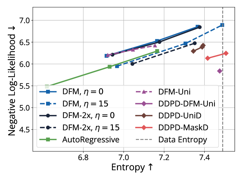
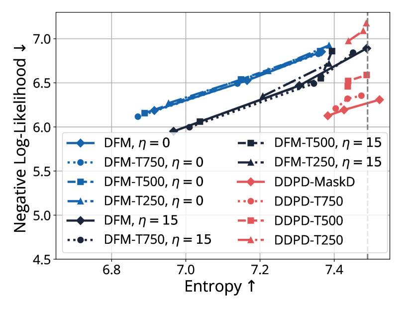
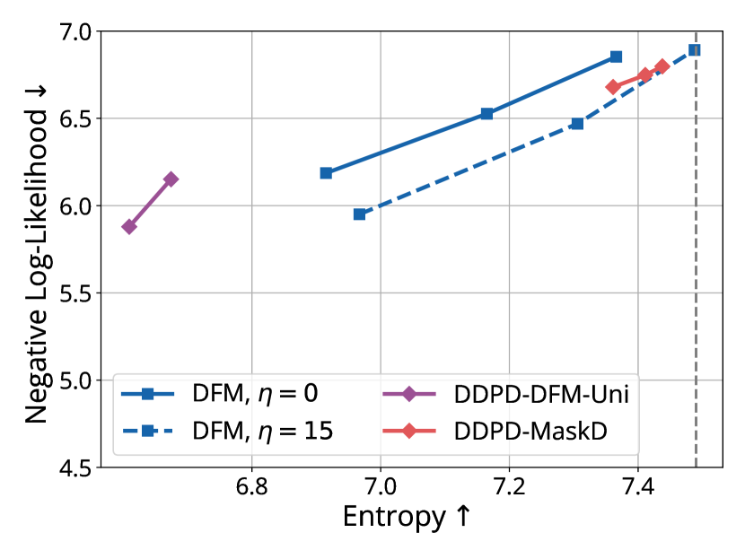
Figure 2: Negative log-likelihood measured with GPT-J versus sample entropy (in terms of tokens), with logit temperatures of the denoiser swept over $\{0.8,0.9,1.0\}$. Left: DDPD v.s. SOTA baselines. Middle: Varying sampling steps from $250$ to $1000$; both DFM and DDPD use the same mask-based denoiser. Right: DDPD single-neural-network v.s. DDPD planner + mask denoiser, both trained for $20k$ iterations. DFM at $750k$ iter.

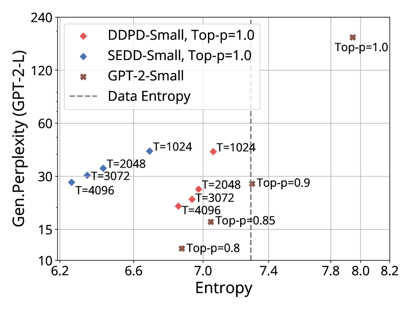
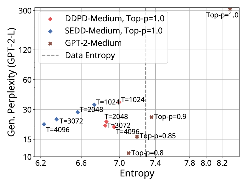
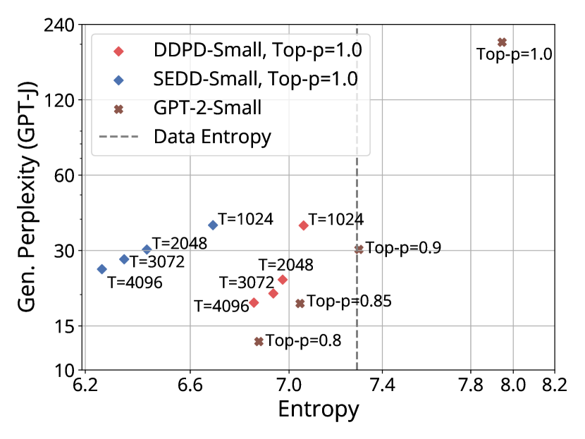
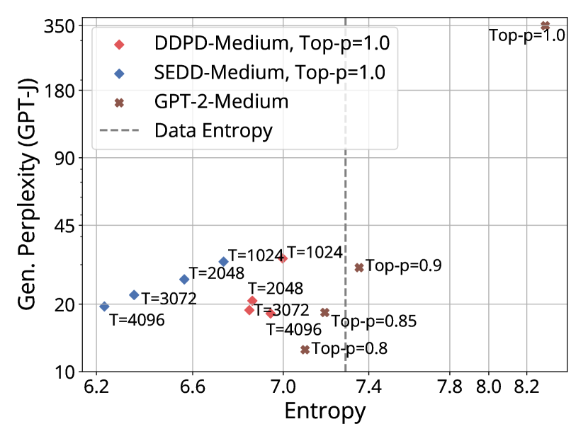
Figure 10: Using $\text{softmax}(\texttt{logit\_if\_noise})$ for planning. Generative perplexity evaluated with GPT-2 Large (GPT-2-L) and GPT-J: SEDD v.s. DDPD using the same denoiser.

OpenWebText Language Modeling.  In Fig. 3, we compare DDPD with SEDD [29], both trained on the larger OpenWebText dataset [18]. We maintained the same experimental settings as in SEDD, with token vocabulary size $S=50257$ and $D=1024$, to validate whether planning improves generative performance under controlled conditions. We use the same pretrained SEDD-small or SEDD-medium score model as a mask diffusion denoiser, based on the conversion relationship outlined in Table 1. A separate planner network, with the same configuration as SEDD-small (90M), is trained for $400k$ iterations with batch size $512$. We evaluated the quality of unconditional samples using generative perplexity, measured by larger language models GPT-2-L (774M) [33] and GPT-J (6B) [40]. Both SEDD and DDPD were simulated using 1024 to 4096 steps, with $\text{top-p}=1.0$. SEDD used tau-leaping, while DDPD employed our newly proposed sampler. We also include GPT-2 [33] as the autoregressive baseline, with top-p sweeping from $0.7$ to $1.0$. We experimented DDPD sampler with both softmax selection (Fig. 10) and proportional selection (Fig. 11).

SEDD shows marginal improvement with additional steps, similar to DFM in the text8 case. In contrast, DDPD leveraged planning to continuously improve sample quality, with the most improvements in early stages and diminishing returns in later steps as the sequence gets mostly corrected. This shows that the planner optimally selects the denoising order and adaptively corrects accumulated mistakes.

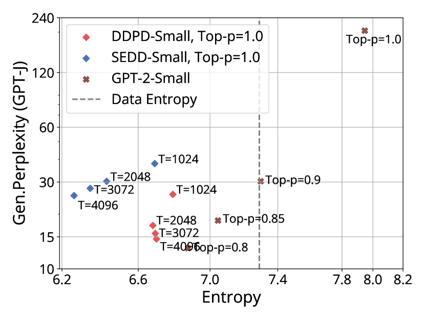
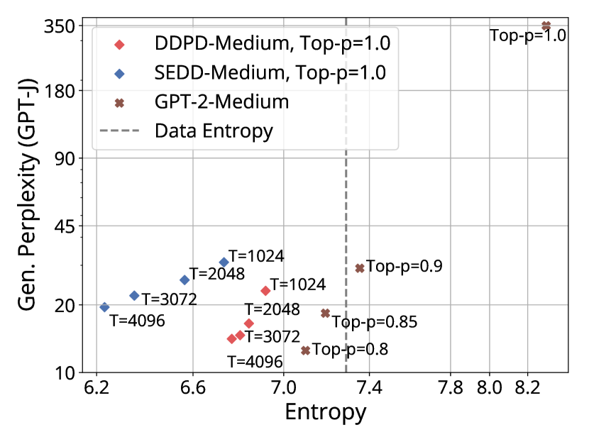
Figure 3: Generative perplexity $\downarrow$ v.s. entropy $\uparrow$ (both plotted in log-scale) of SEDD, DDPD and GPT-2.

ImageNet $256\times 256$ Generation with Discrete Tokens.  An image is represented using discrete-valued tokens with a pre-trained tokenizer and a decoder. The generative model is used for generating sequences in the token space. We focus on understanding how DDPD compares to existing sampling methods using the same denoiser, instead of aiming for SOTA performance. The pretrained tokenizer and mask denoiser from Yu et al. [45] is used, where the token length of an image is $D=128$.

We compare DDPD with two mask diffusion type baselines: 1) standard mask diffusion and 2) MaskGIT [8], which selects the next tokens based on the denoiser’s confidence of its predicted logits. To prevent MaskGIT from making overly greedy selections, random noise is added to the confidence scores, with its magnitude annealed to zero following a linear schedule. We test all methods from $8$ to $128$ steps. Parallel sampling is used if $\#\,\text{steps}<128$. The results on FID scores ([19], lower is better) are presented in Table 2. More results on inception scores and comparison with SOTA are in Section E.3. Generated samples are in Section F.3. In DDPD, the sampling process is divided into two stages: the first half follows a parallel sampling schedule, while the second half adopts an adaptive step size based on the noise level, allowing for finer discretization towards the end of sampling.

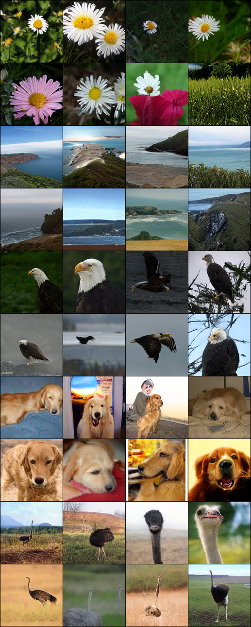
(a) DDPD $16+16$ steps

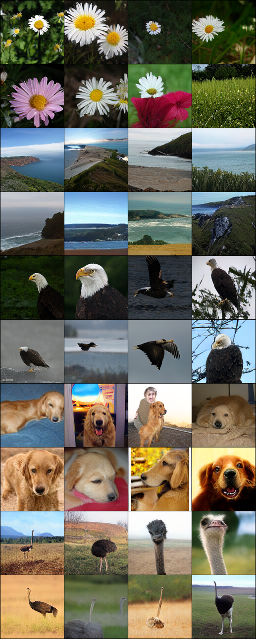
(b) DDPD $16+32$ steps

Figure 13: DDPD No Annealing, increasing number of refinement steps. The added refinement steps act as “touch-up” to improve the aesthetic quality without losing its original content.

Notably, we observe that the standard mask performs poorly, with no significant improvement even with more sampling steps. This is attributed to the low accuracy of the denoiser, which is much worse than in OpenWebText language modeling ($3\%$ v.s. $60\%$ at $t=0.85$). The confidence-based sampling of MaskGIT proves effective, but its greedy selection, despite the added randomness, sacrifices the sample diversity for quality, leading to higher FID values compared to DDPD. This issue becomes particularly pronounced when more steps are used, resulting in an overly greedy sampling order. While DDPD requires a minimum number of sampling steps to correct sampling errors from earlier stages, it achieves the best results and more steps do not lead to worse FID. We also conducted ablation to study the effect of increasing number of second-stage steps for DDPD in Fig. 13.

To enhance the empirical performance in image token generation, we tested all methods with logit temperature annealing, a common approach to lower sampling temperature $\tau$ for improved denoising accuracy. We found $\tau=0.6$ gives the best results among $\tau=1.0,0.9,0.8,0.7,0.6,0.5$, greatly improving mask diffusion and resulting in competitive FID scores. However, for MaskGIT, this reduces sample diversity, leading to even higher FID scores compared to no annealing. We also tried another annealing trick from Yu et al. [45], where $\tau$ is linearly reduced from $1.0$ to $0.0$ during generation. This trick worked well for mask diffusion, allowing for further improvement over fixed-temperature annealing. For DDPD, performance remained relatively stable, with minor improvements or degradations compared to no annealing.

Table 2: FID score ($\downarrow$) on ImageNet $256\times 256$. MaskD refers to mask diffusion. The denoiser and parallel sampling schedule are kept the same as [45], without classifier-free guidance.

	No Logit Annealing			Logit temp $0.6$			Logit temp $1.0$ $\rightarrow$ $0.0$
Steps $T$	MaskD	MaskGIT	DDPD	MaskD	MaskGIT	DDPD	MaskD	MaskGIT	DDPD
$8$	38.06	5.51	6.8	5.69	10.02	5.71	4.99	8.53	5.99
$16$	32.44	6.66	5.12	4.85	11.24	4.92	4.69	9.21	5.03
$32$	29.12	8.09	4.75	4.86	11.93	4.91	4.62	9.9	4.98
$64$	27.54	9.08	4.73	4.98	12.26	5.14	4.6	10.35	5.26
$128$	26.83	9.34	4.89	5.13	12.52	5.39	4.89	10.2	5.54

7 Conclusion

We introduced Discrete Diffusion with Planned Denoising (DDPD), a novel framework that decomposes the discrete generation process into planning and denoising. We propose a new adaptive sampler that leverages the planner for more effective and robust generation by adjusting time step sizes and prioritizing the denoising of the most corrupted positions. Additionally, it simplifies the learning process by allowing each model to focus specifically on either planning or denoising. The incorporation of planning makes the generative process more robust to errors made by the denoiser during generation. On GPT-2 scale language modeling and ImageNet $256\times 256$ token generation, DDPD enables a significant performance boost compared to denoiser-only discrete diffusion models.

Acknowledgments

We thank Jiaxin Shi for valuable discussions on evaluation of ELBO. SL and RGB acknowledge funding from MIT-IBM Watson AI Lab, NSF Award 2209892 and compute from NERSC GenAI award m4737. JN acknowledges support from Toyota Research Institute. AC acknowledges support from the EPSRC CDT in Modern Statistics and Statistical Machine Learning (EP/S023151/1).

Appendix

Appendix A Proofs

A.1 Proof of Proposition 3.1

Part 1: Calculate $p\left(z_{t}^{d}=N|x_{t}\right)$ in Eq. 10.

We first derive how to calculate $p\left(z_{t}^{d}=N|x_{t}\right)$ in Eq. 10 using $p_{1|t}$.

First, from law of total probability,

$$p\left(z_{t}^{d}=N|x_{t}\right)=\sum_{\bar{j}^{d}}p_{1|t}\left(x_{1}^{d}=\bar{j}^{d}|x_{t}\right)p\left(z_{t}^{d}=N|x_{1}^{d}=\bar{j}^{d},x_{t}\right)$$ (16)

Next we derive closed form of $p\left(z_{t}^{d}=N|x_{1}^{d}=\bar{j}^{d},x_{t}\right)$.

According to the noise schedule,

$$p\left(z_{t}^{d},x_{t}^{d}|x_{1}\right) =\begin{cases}\alpha_{t}&\text{if}\,\,z_{t}^{d}=D,x_{t}^{d}=x_{1}^{d}\\ 0&\text{if}\,\,z_{t}^{d}=D,x_{t}^{d}\neq x_{1}^{d}\\ \nicefrac{{\left(1-\alpha_{t}\right)}}{{S}}&\text{if}\,\,z_{t}^{d}=N,x_{t}^{d}=x_{1}^{d}\\ \nicefrac{{\left(1-\alpha_{t}\right)}}{{S}}&\text{if}\,\,z_{t}^{d}=N,x_{t}^{d}\neq x_{1}^{d}\\ \end{cases}$$ (17)

Using Bayes rule $p\left(z_{t}^{d}|x_{t}^{d},x_{1}\right)=p\left(z_{t}^{d},x_{t}^{d}|x_{1}\right)/p\left(x_{t}^{d}|x_{1}\right)$, we have

$$p\left(z_{t}^{d}|x_{t}^{d},x_{1}\right) =\begin{cases}\frac{\alpha_{t}}{\alpha_{t}+{\left(1-\alpha_{t}\right)}/{S}}&\text{if}\,\,z_{t}^{d}=D,x_{t}^{d}=x_{1}^{d}\\ 0&\text{if}\,\,z_{t}^{d}=D,x_{t}^{d}\neq x_{1}^{d}\\ \frac{{\left(1-\alpha_{t}\right)}/{S}}{\alpha_{t}+{\left(1-\alpha_{t}\right)}/{S}}&\text{if}\,\,z_{t}^{d}=N,x_{t}^{d}=x_{1}^{d}\\ 1&\text{if}\,\,z_{t}^{d}=N,x_{t}^{d}\neq x_{1}^{d}\\ \end{cases}$$ (18)

Plugging Eq. 18 into Eq. 16, we have

$$p\left(z_{t}^{d}=N|x_{t}\right) =\sum_{\bar{j}^{d}}p\left(x_{1}^{d}=\bar{j}^{d}|x_{t}\right)p\left(z_{t}^{d}=N|x_{1}^{d}=\bar{j}^{d},x_{t}\right)$$ (19)

$$=\sum_{\bar{j}^{d}\neq x_{t}^{d}}p\left(x_{1}^{d}=\bar{j}^{d}|x_{t}\right)\cdot 1+p\left(x_{1}^{d}=x_{t}^{d}|x_{t}\right)\cdot\frac{{\left(1-\alpha_{t}\right)}/{S}}{\alpha_{t}+{\left(1-\alpha_{t}\right)}/{S}}$$ (20)

$$=\sum_{\bar{j}^{d}\neq x_{t}^{d}}p\left(x_{1}^{d}=\bar{j}^{d}|x_{t}\right)\cdot 1+p\left(x_{1}^{d}=x_{t}^{d}|x_{t}\right)\cdot\left(1-\frac{\alpha_{t}}{\alpha_{t}+{\left(1-\alpha_{t}\right)}/{S}}\right)$$ (21)

$$=1-p\left(x_{1}^{d}=x_{t}^{d}|x_{t}\right)\frac{\alpha_{t}}{\alpha_{t}+{\left(1-\alpha_{t}\right)}/{S}}$$ (22)

which gives us the form in Eq. 10.

Part 2: Calculate $p_{1|t}\left(x_{1}^{d}=j^{d}|x_{t},z_{t}^{d}=N\right)$ in Eq. 11.

From Bayes rule, we have

$$p_{1|t}\left(x_{1}^{d}=j^{d}|x_{t},z_{t}^{d}=N\right) =\frac{p\left(x_{1}^{d}=j^{d},z_{t}^{d}=N|x_{t}\right)}{p\left(z_{t}^{d}=N|x_{t}\right)}$$ (23)

$$=\frac{p\left(x_{1}^{d}=j^{d}|x_{t}\right)p\left(z_{t}^{d}=N|x_{t},x_{1}^{d}=j^{d}\right)}{p\left(z_{t}^{d}=N|x_{t}\right)}$$ (24)

$$=\frac{p\left(x_{1}^{d}=j^{d}|x_{t}\right)}{p\left(z_{t}^{d}=N|x_{t}\right)},\quad\forall x_{t}^{d}\neq j^{d}$$ (25)

Eq. 25 is by plugging in the following from Eq. 18 that $p\left(z_{t}^{d}=N|x_{t},x_{1}^{d}=j^{d}\right)=1$ if $x_{t}^{d}\neq j^{d}$.

Part 3: Verify equivalence to the original optimal rate in Eq. 9.

By plugging in Eq. 10 and Eq. 11 into Eq. 9, we have

$$R_{t}^{\mathrm{unif}}\left(x_{t},j^{d}\right)=\underbrace{\frac{\dot{\alpha_{t}}}{1-\alpha_{t}}}_{\text{recovery rate}}\underbrace{p\left(z_{t}^{d}=N|x_{t}\right)}_{\text{prob. of corruption}}\underbrace{p_{1|t}\left(x_{1}^{d}=j^{d}|x_{t},z_{t}^{d}=N\right)}_{\text{prob. of denoising}}=\underbrace{\frac{\dot{\alpha_{t}}}{1-\alpha_{t}}}_{\text{recovery rate}}\underbrace{p_{1|t}\left(x_{1}^{d}=j^{d}|x_{t}\right)}_{\text{composed denoising prob.}}$$ (26)

A.2 Proof of Theorem 4.1: Deriving the ELBO for training

This derivation follows the Continuous Time Markov Chain framework. We refer the readers to Appendix C.1 of Campbell et al. [7] for a primer on CTMC. Here we provide the proof for $D=1$ case. The result holds for $D>1$ case following same arguments from Appendix E of Campbell et al. [7].

Let $W$ be a CTMC trajectory, fully described by its jump times $T_{1},\cdots,T_{n}$ and state values between jumps $W_{0},W_{T_{0}},\cdots,W_{T_{n}}$. At time $T_{k}$, the state jumps from $W_{T_{k-1}}$ to $W_{T_{k}}$. With its path measure properly defined, we start with the following result from Campbell et al. [7] Appendix C.1, the ELBO of $\mathbb{E}_{p_{\mathrm{data}}(x_{1})}\left[\log p_{\theta}(x_{1})\right]$ is given by introducing the corruption process as the variational distribution:

$$\mathbb{E}_{p_{\mathrm{data}}(x_{1})}\left[\log p_{\theta}(x_{1})\right]\geq\int p_{\mathrm{data}}(\mathrm{d}x_{1})\mathbb{Q}^{|x_{1}}(\mathrm{d}\omega)\log\frac{\mathrm{d}\mathbb{P}^{\theta}}{\mathrm{d}\mathbb{Q}^{|x_{1}}}(\omega),$$ (27)

where

$$\frac{\mathrm{d}\mathbb{P}^{\theta}}{\mathrm{d}\mathbb{Q}^{|x_{1}}}(\omega)=\frac{p_{0}(W_{0})\exp\left(-\int_{t=0}^{t=1}R_{t}^{\theta}(W_{t}^{-})\mathrm{d}t\right)\prod_{t:W_{t}\neq W_{t}^{-}}R_{t}^{\theta}(W_{t}^{-},W_{t})}{p_{0|1}(W_{0}|x_{1})\exp\left(-\int_{t=0}^{t=1}R_{t}(W_{t}^{-}|x_{1})\mathrm{d}t\right)\prod_{t:W_{t}\neq W_{t}^{-}}R_{t}(W_{t}^{-},W_{t}|x_{1})}.$$ (28)

Intuitively, the measure (probability) of a trajectory is determined by: the starting state from the prior distribution $p_{0}(W_{0})$, and the product of the probability of waiting from $T_{k-1}$ to $T_{k}$ (which follows an Exponential distribution) and the transition rate of the jump from $W_{t}^{-}$ to $W_{t}$.

For our method, when simulating the data corruption process, we augment $W_{t}^{\text{aug}}$ to record both state values $W_{t}$ and its latent value $Z_{t}\in\{N,D\}^{D}$. The jump is defined to happen when the latent value jumps from $Z_{k-1}$ to $Z_{k}$ with one of the dimensions corrupted and the state value jumps from $W_{k-1}$ to $W_{k}$. Similarly, the ELBO of $\mathbb{E}_{p_{\mathrm{data}}(x_{1})}\left[\log p_{\theta}(x_{1})\right]$ can be defined as:

$$\mathbb{E}_{p_{\mathrm{data}}(x_{1})}\left[\log p_{\theta}(x_{1})\right]\geq\int p_{\mathrm{data}}(\mathrm{d}x_{1})\mathbb{Q}^{|x_{1}}(\mathrm{d}\omega^{\text{aug}})\log\frac{\mathrm{d}\mathbb{P}^{\theta}}{\mathrm{d}\mathbb{Q}^{|x_{1}}}(\omega^{\text{aug}})$$ (29)

where the Radon-Nikodym derivative is given by:

$$\frac{\mathrm{d}\mathbb{P}^{\theta}}{\mathrm{d}\mathbb{Q}^{\mid x_{1}}}(\omega^{\text{aug}})=\frac{p_{0}\left(W_{0}\right)\exp\left(-\int_{t=0}^{t=1}R_{t}^{\theta}\left(W_{t}^{-}\right)\mathrm{d}t\right)\prod_{t}R_{t}^{\theta}\left(W_{t}^{-},W_{t}\right)}{p_{0\mid 1}\left(W_{0},Z_{0}\mid x_{1}\right)\exp\left(-\int_{t=0}^{t=1}R_{t}\left(W_{t}^{-},Z_{t}^{-}\mid x_{1}\right)\mathrm{d}t\right)\prod_{t}R_{t}\left(W_{t}^{-},W_{t},Z_{t}^{-},Z_{t}\mid x_{1}\right)}$$ (30)

By plugging in Eq. 30 into Eq. 29, we arrive at

$$\mathcal{L}_{\text{ELBO }} =\int p_{\mathrm{data}}\left(\mathrm{d}x_{1}\right)\int_{\omega^{\text{aug}}:\mathbb{Q}^{\mid x_{1}}(\omega^{\text{aug}})>0}\mathbb{Q}^{\mid x_{1}}(\mathrm{d}\omega^{\text{aug}})\left\{-\int_{t=0}^{t=1}{R}_{t}^{\theta}\left(W_{t}^{-}\right)\mathrm{d}t+\sum_{t}\log{R}_{t}^{\theta}\left(W_{t}^{-},W_{t}\right)\right\}$$

$$=\int p_{\mathrm{data}}\left(\mathrm{d}x_{1}\right)\int_{\omega^{\text{aug}}:\mathbb{Q}^{\mid x_{1}}(\omega^{\text{aug}})>0}\mathbb{Q}^{\mid x_{1}}(\mathrm{d}\omega^{\text{aug}})\Bigg{\{}-\int_{t=0}^{t=1}\frac{\dot{\alpha_{t}}}{1-\alpha_{t}}p_{\theta}\left(Z_{t}^{-}=N|W_{t}^{-}\right)$$

$$+\sum_{t}\log\frac{\dot{\alpha_{t}}}{1-\alpha_{t}}p_{\theta}\left(Z_{t}^{-}=N|W_{t}^{-}\right)p_{1|t}^{\theta}\left(x_{1}=W_{t}|W_{t}^{-},Z_{t}^{-}=N\right)\Bigg{\}}$$

$$=\int p_{\mathrm{data}}\left(\mathrm{d}x_{1}\right)\int_{\omega^{\text{aug}}:\mathbb{Q}^{\mid x_{1}}(\omega^{\text{aug}})>0}\mathbb{Q}^{\mid x_{1}}(\mathrm{d}\omega^{\text{aug}})\Bigg{\{}-\int_{t=0}^{t=1}\frac{\dot{\alpha_{t}}}{1-\alpha_{t}}p_{\theta}\left(Z_{t}^{-}=N|W_{t}^{-}\right)$$

$$+\sum_{t\in\{T_{1},\cdots,T_{N}\}}\left(\log\frac{\dot{\alpha_{t}}}{1-\alpha_{t}}p_{\theta}\left(Z_{t}^{-}=N|W_{t}^{-}\right)+\log p_{1|t}^{\theta}\left(x_{1}=W_{t}|W_{t}^{-},Z_{t}^{-}=N\right)\right)\Bigg{\}}$$ (31)

Eq. 31 contain terms that depend on the planner $p_{\theta}\left(z_{t}=N|x_{t}\right)$ and the denoiser $p_{1|t}^{\theta}\left(x_{1}=j|x_{t},z_{t}=N\right)$. Next, we show those terms can be separated into two parts:

$$\mathcal{L}_{\text{denoiser}} =\mathbb{E}_{\mathcal{U}(t;0,1)p_{\mathrm{data}}\left(x_{1}\right)p\left(x_{t},z_{t}\mid x_{1}\right)}\left[\frac{\dot{\alpha_{t}}}{1-\alpha_{t}}\delta\{z_{t},N\}\log p_{1|t}^{\theta}({x}_{1}|x_{t},z_{t}=N)\right]$$ (32)

$$\mathcal{L}_{\text{planner}} =\mathbb{E}_{\mathcal{U}(t;0,1)p_{\mathrm{data}}(x_{1})p_{t|1}\left(z_{t},x_{t}\mid x_{1}\right)}\left[\frac{\dot{\alpha_{t}}}{1-\alpha_{t}}\log p_{\theta}\left(z_{t}|x_{t}\right)\right]$$ (33)

First part: cross-entropy loss on $x_{1}$ denoising.

All terms associated with $p_{1|t}^{\theta}\left(x_{1}=W_{t}|W_{t}^{-},Z_{t}^{-}=N\right)$ are:

$$\mathcal{L}_{\text{denoising}} =\int p_{\mathrm{data}}\left(\mathrm{d}x_{1}\right)\int_{\omega^{\text{aug}}}\mathbb{Q}^{\mid x_{1}}(\mathrm{d}\omega^{\text{aug}})\sum_{t}\log p_{1|t}^{\theta}\left(x_{1}=W_{t}|W_{t}^{-},Z_{t}^{-}=N\right)$$

$$=\int p_{\mathrm{data}}\left(\mathrm{d}x_{1}\right)\int_{\omega^{\text{aug}}}\mathbb{Q}^{\mid x_{1}}(\mathrm{d}\omega^{\text{aug}})\int_{t=0}^{t=1}\sum_{(y,u)}R_{t}\left((W_{t},Z_{t}),(y,u)|x_{1}\right)\log p_{1|t}^{\theta}\left(x_{1}=W_{t}|W_{t}^{-},Z_{t}^{-}=N\right)\;\text{Dynkin}$$

$$=\int p_{\mathrm{data}}\left(\mathrm{d}x_{1}\right)\int_{\omega^{\text{aug}}}\mathbb{Q}^{\mid x_{1}}(\mathrm{d}\omega^{\text{aug}})\int_{t=0}^{t=1}\sum_{(y,u)}\frac{\dot{\alpha_{t}}}{1-\alpha_{t}}\delta\{Z_{t},N\}\delta\{u,D\}\delta\{y,x_{1}\}\log p_{1|t}^{\theta}\left(x_{1}=W_{t}|W_{t}^{-},Z_{t}^{-}=N\right)$$

$$=\int\int_{t=0}^{t=1}p_{\mathrm{data}}\left(\mathrm{d}x_{1}\right)\int_{\omega^{\text{aug}}}\mathbb{Q}^{\mid x_{1}}(\mathrm{d}\omega^{\text{aug}})\frac{\dot{\alpha_{t}}}{1-\alpha_{t}}\delta\{Z_{t},N\}\log p_{1|t}^{\theta}\left(x_{1}=W_{t}|W_{t}^{-},Z_{t}^{-}=N\right)$$

$$=\mathbb{E}_{\mathcal{U}(t;0,1)p_{\mathrm{data}}\left(x_{1}\right)p_{t|1}\left(z_{t},x_{t}\mid x_{1}\right)}\left[\frac{\dot{\alpha_{t}}}{1-\alpha_{t}}\delta\{z_{t},N\}\log p_{1|t}^{\theta}\left(x_{1}|x_{t},z_{t}=N\right)\right]$$

At the second equation, we use Dynkin’s formula

$$\int p_{\mathrm{data}}\left(\mathrm{d}x_{1}\right)\mathbb{Q}^{\mid x_{1}}(\mathrm{d}\omega)\sum_{t:\text{all jump times}}f\left(W_{t}^{-},W_{t}\right)=\int p_{\mathrm{data}}\left(\mathrm{d}x_{1}\right)\mathbb{Q}^{\mid x_{1}}(\mathrm{d}\omega)\int_{t=0}^{t=1}\sum_{y}R_{t}\left(W_{t},y\mid x_{1}\right)f\left(W_{t},y\right)\mathrm{d}t$$

which allows us to switch from a sum over jump times into a full integral over time interval weighted by the probability of the jump happening and the next state the jump goes to.

Second part: cross-entropy loss on $z_{t}=N$ prediction.

The remaining terms are associated with $\frac{\dot{\alpha_{t}}}{1-\alpha_{t}}p_{\theta}\left(Z_{t}^{-}=N|W_{t}^{-}\right)$ which is the jump rate at $W_{t}^{-}$, i.e. $R_{t,\text{jump}}^{\theta}(W_{t}^{-})=\sum_{j}R_{t,\text{jump}}^{\theta}(W_{t}^{-},j)=\frac{\dot{\alpha_{t}}}{1-\alpha_{t}}p_{\theta}\left(Z_{t}^{-}=N|W_{t}^{-}\right)$ according to Eq. 12. In this proof, we will use $R_{t}^{\theta}$ in short for $R_{t,\text{jump}}^{\theta}$. The remaining loss terms

$$\mathcal{L}_{\text{planner}} =\int p_{\mathrm{data}}\left(\mathrm{d}x_{1}\right)\int_{\omega^{\text{aug}}}\mathbb{Q}^{|x_{1}}(\mathrm{d}\omega^{\text{aug}})\left\{-\int_{t=0}^{t=1}R_{t}^{\theta}\left(W_{t}^{-}\right)\mathrm{d}t+\sum_{t}\log R_{t}^{\theta}\left(W_{t}^{-}\right)\right\}$$

$$=\int p_{\mathrm{data}}\left(\mathrm{d}x_{1}\right)\int_{\omega^{\text{aug}}}\mathbb{Q}^{|x_{1}}(\mathrm{d}\omega^{\text{aug}})\left\{-\int_{t=0}^{t=1}R_{t}^{\theta}\left(W_{t}\right)\mathrm{d}t+\int_{t=0}^{t=1}\sum_{(y,u)}R_{t}\left((W_{t},Z_{t}),(y,u)|x_{1}\right)\log R_{t}^{\theta}\left(W_{t}\right)\mathrm{d}t\right\}$$

Dynkin

$$=\int p_{\mathrm{data}}\left(\mathrm{d}x_{1}\right)\int_{\omega^{\text{aug}}}\mathbb{Q}^{|x_{1}}(\mathrm{d}\omega^{\text{aug}})\left\{-\int_{t=0}^{t=1}R_{t}^{\theta}\left(W_{t}\right)\mathrm{d}t+\int_{t=0}^{t=1}\frac{\dot{\alpha_{t}}}{1-\alpha_{t}}\delta\{Z_{t},N\}\log R_{t}^{\theta}\left(W_{t}\right)\mathrm{d}t\right\}$$

$$=\mathbb{E}_{\mathcal{U}(t;0,1)p_{\mathrm{data}}(x_{1})p\left(x_{t},z_{t}|x_{1}\right)}\left[-R_{t}^{\theta}\left(x_{t}\right)+\frac{\dot{\alpha_{t}}}{1-\alpha_{t}}\delta\{z_{t},N\}\log R_{t}^{\theta}\left(x_{t}\right)\right]$$

We first rewrite the loss as

$$\mathbb{E}_{\mathcal{U}(t;0,1)p(x_{t})p\left(x_{1},z_{t}|x_{t}\right)}\left[-R_{t}^{\theta}\left(x_{t}\right)+\frac{\dot{\alpha_{t}}}{1-\alpha_{t}}\delta\{z_{t},N\}\log R_{t}^{\theta}\left(x_{t}\right)\right]$$

$$= \mathbb{E}_{\mathcal{U}(t;0,1)p(x_{t})p\left(x_{1},z_{t}|x_{t}\right)}\left[-\frac{\dot{\alpha_{t}}}{1-\alpha_{t}}p_{\theta}\left(z_{t}=N|x_{t}\right)+\frac{\dot{\alpha_{t}}}{1-\alpha_{t}}\delta\{z_{t},N\}\log\frac{\dot{\alpha_{t}}}{1-\alpha_{t}}p_{\theta}\left(z_{t}=N|x_{t}\right)\right]$$ (34)

If $x_{t}$ is given fixed, by taking the derivative of $p_{\theta}\left(z_{t}=N|x_{t}\right)$ and setting it to zero, we have the optimal solution to be:

$$p_{\theta}\left(z_{t}=N|x_{t}\right)=\mathbb{E}_{p\left(x_{1},z_{t}\mid x_{t}\right)}\delta\{z_{t},N\}$$

This is equivalent to optimizing the cross-entropy loss, which has the same optimal solution:

$$\mathbb{E}_{p\left(x_{1},z_{t}\mid x_{t}\right)}\left[\delta\{z_{t},N\}\log p_{\theta}\left(z_{t}=N|x_{t}\right)+\left(1-\delta\{z_{t},N\}\right)\log\left(1-p_{\theta}\left(z_{t}=N|x_{t}\right)\right)\right]$$

Plugging this $x_{t}$-conditional loss back to Eq. 34, we arrive at the cross entropy training loss for the planner:

$$\mathcal{L}_{\text{planner}}=\mathbb{E}_{\mathcal{U}(t;0,1)p_{\mathrm{data}}(x_{1})p_{t|1}\left(z_{t},x_{t}\mid x_{1}\right)}\left[\frac{\dot{\alpha_{t}}}{1-\alpha_{t}}\log p_{\theta}\left(z_{t}|x_{t}\right)\right].$$

A.3 Proof of Proposition 3.3: Continuous Time Markov Chains with Self-Connections

We first describe the stochastic process that includes self-loops as this differs slightly from the standard CTMC formulation. We have a rate matrix $\tilde{R}(i,j)$ that is non-negative at all entries, $\tilde{R}(i,j)\geq 0$. To simulate this process, we alternate between waiting for an exponentially distributed amount of time and sampling a next state from a transition distribution. The waiting time is exponentially distributed with rate $\sum_{k}\tilde{R}(i,k)$. The next state transition distribution is $\tilde{P}(j|i)=\frac{\tilde{R}(i,j)}{\sum_{k}\tilde{R}(i,k)}$. Note that $\tilde{P}(i|i)$ can be non-zero due to the self-loops in this style of process.

We can find an equivalent CTMC without self-loops that has the same distribution over trajectories as this self-loop process. To find this, we look at the infinitesimal transition distribution from time $t$ to time $t+\Delta t$. We let $J$ denote the event that the exponential timer expires during the period $[t,t+\Delta t]$. We let $\bar{J}$ denote the no jump event. For the self-loop process, the infinitesimal transition distribution is

$$p_{t+\Delta t|t}(j|i) =\mathbb{P}(J,j|i)+\mathbb{P}(\bar{J},j|i)$$

$$=\mathbb{P}(J|i)\mathbb{P}(j|J,i)+\mathbb{P}(\bar{J}|i)\mathbb{P}(j|\bar{J},i)$$

We have the following relations

$$\mathbb{P}(J|i) =\sum_{k}\tilde{R}(i,k)\Delta t\quad\text{property of exponential distribution}$$

$$\mathbb{P}(j|J,i) =\frac{\tilde{R}(i,j)}{\sum_{k}\tilde{R}(i,k)}$$

$$\mathbb{P}(j|\bar{J},i) =\delta\{j=i\}$$

Our infinitesimal transition distribution therefore becomes

$$p_{t+\Delta t|t}(j|i) =\left(\sum_{k}\tilde{R}(i,k)\Delta t\right)\frac{\tilde{R}(i,j)}{\sum_{k}\tilde{R}(i,k)}+\left(1-\Delta t\sum_{k}\tilde{R}(i,k)\right)\delta\{j=i\}$$

$$=\Delta t\tilde{R}(i,j)+\delta\{j=i\}-\delta\{j=i\}\Delta t\sum_{k}\tilde{R}(i,k)$$

$$=\delta\{i=j\}+\Delta t\left(\tilde{R}(i,j)-\delta\{i=j\}\sum_{k}\tilde{R}(i,k)\right)$$

We now note that for a standard CTMC without self-loops and rate matrix $R(i,j)$, the infinitesimal transition probability is

$$p_{t+\Delta t|t}(j|i)=\delta\{i=j\}+\Delta tR(i,j)$$

Therefore, we can see our self-loop process is equivalent to the CTMC with rate matrix equal to

$$R(i,j) =\tilde{R}(i,j)\quad i\neq j$$

$$R(i,i) =-\sum_{k}\tilde{R}(i,k)$$

In other words, the CTMC rate matrix is the same as the self-loop matrix except simply removing the diagonal entries and replacing them with negative row sums as is standard.

In our case, the original CTMC without self-loops is defined by rate matrix

$$R_{t}(x_{t},j^{d})=\frac{\dot{\alpha}_{t}}{1-\alpha_{t}}p_{\theta}(z_{t}^{d}=N|x_{t})p_{1|t}^{\theta}(x_{1}^{d}=j^{d}|x_{t},z_{t}^{d}=N),\qquad\forall x_{t}^{d}\neq j^{d}$$

We have free choice over the diagonal entries in our self-loop rate matrix and so we set the diagonal entries to be exactly the above equation evaluated at $x_{t}^{d}=j^{d}$.

$$\tilde{R}_{t}(x_{t},j^{d})=\frac{\dot{\alpha}_{t}}{1-\alpha_{t}}p_{\theta}(z_{t}^{d}=N|x_{t})p_{1|t}^{\theta}(x_{1}^{d}=j^{d}|x_{t},z_{t}^{d}=N),\forall x_{t}^{d},j^{d}$$

We can now evaluate the quantities needed for Gillespie’s Algorithm. The first is the total jump rate

$$\sum_{d}\sum_{j^{d}}\tilde{R}_{t}(x_{t},j^{d}) =\frac{\dot{\alpha}_{t}}{1-\alpha_{t}}\sum_{d}\sum_{j^{d}}p_{\theta}(z_{t}^{d}=N|x_{t})p_{1|t}^{\theta}(x_{1}=j^{d}|x_{t},z_{t}^{d}=N)$$ (35)

$$=\frac{\dot{\alpha}_{t}}{1-\alpha_{t}}\sum_{d}p_{\theta}(z_{t}^{d}=N|x_{t})$$ (36)

We now need to find the next state jump distribution. To find the dimension to jump to we use

$$\frac{\sum_{j^{d}}\tilde{R}_{t}(x_{t},j^{d})}{\sum_{d}\sum_{j^{d}}\tilde{R}_{t}(x_{t},j^{d})}=\frac{\frac{\dot{\alpha}_{t}}{1-\alpha_{t}}p_{\theta}(z_{t}^{d}=N|x_{t})}{\frac{\dot{\alpha_{t}}}{1-\alpha_{t}}}=p_{\theta}(z_{t}^{d}=N|x_{t})$$ (37)

To find the state within the chosen jump, the distribution is

$$\frac{\tilde{R}_{t}(x_{t},j^{d})}{\sum_{j^{d}}\tilde{R}_{t}(x_{t},j^{d})} =\frac{\frac{\dot{\alpha}_{t}}{1-\alpha_{t}}p_{\theta}(z_{t}^{d}=N|x_{t})p_{1|t}^{\theta}(x_{1}^{d}=j^{d}|x_{t},z_{t}^{d}=N)}{\frac{\dot{\alpha}_{t}}{1-\alpha_{t}}p_{\theta}(z_{t}^{d}=N|x_{t})}$$ (38)

$$=p_{1|t}^{\theta}(x_{1}^{d}=j^{d}|x_{t},z_{t}^{d}=N)$$ (39)

Appendix B General formulation

B.1 Score-entropy based: SDDM [39], SEDD [29]

For coherence, we assume $t=0$ is noise and $t=1$ is data, while discrete diffusion literature consider a flipped notion of time. Following Campbell et al. [6], (see Sec. H.1 of Campbell et al. [7]), the conditional reverse rate of discrete diffusion considered in [39; 29] is defined to be:

$$R_{t}^{\text{diff }}\left(x_{t},j^{d}\mid x_{1}^{d}\right)=R_{t}(j^{d},x_{t}^{d})\frac{p_{t\mid 1}\left(j^{d}\mid x_{1}^{d}\right)}{p_{t\mid 1}\left(x_{t}^{d}\mid x_{1}^{d}\right)}$$ (40)

with the forward corruption rate $R_{t}=\frac{\dot{\alpha_{t}}}{S\alpha_{t}}\left(\mathds{1}\mathds{1}^{\top}-S\mathbf{I}\right)$ for uniform diffusion or $R_{t}=\frac{\dot{\alpha_{t}}}{\alpha_{t}}\left(\mathds{1}\mathbf{e}_{\mathbb{M}}^{\top}-\mathbf{I}\right)$ for mask diffusion, such that the corruption schedule is according to $\alpha_{t}$.

And the expected reverse rate for $x_{t}^{d}\neq j^{d}$ is given by:

$$R_{t}^{\text{diff }}\left(x_{t},j^{d}\right) =\mathbb{E}_{p_{1|t}(x_{1}^{d}\mid x_{t})}R_{t}^{\text{diff }}\left(x_{t},j^{d}\mid x_{1}^{d}\right)$$ (41)

$$=\sum_{x_{1}^{d}}p_{1\mid t}\left(x_{1}^{d}\mid x_{t}\right)R_{t}(j^{d},x_{t}^{d})\frac{p_{t\mid 1}\left(j^{d}\mid x_{1}^{d}\right)}{p_{t\mid 1}\left(x_{t}^{d}\mid x_{1}^{d}\right)}$$ (42)

$$=R_{t}\sum_{x_{1}^{d}}p_{1\mid t}\left(x_{1}^{d}\mid x_{t}\right)\frac{p_{t\mid 1}\left(j^{d}\mid x_{1}^{d}\right)}{p_{t\mid 1}\left(x_{t}^{d}\mid x_{1}^{d}\right)}$$ (43)

$$=R_{t}\sum_{x_{1}^{d}}\frac{p\left(x_{t}^{d}\mid x_{1}^{d},x_{t}^{{\backslash d}}\right)p\left(x_{1}^{d}\mid x_{t}^{{\backslash d}}\right)}{p\left(x_{t}^{d}\mid x_{t}^{{\backslash d}}\right)}\frac{p_{t\mid 1}\left(j^{d}\mid x_{1}^{d}\right)}{p_{t\mid 1}\left(x_{t}^{d}\mid x_{1}^{d}\right)}$$ (44)

$$=R_{t}\sum_{x_{1}^{d}}\frac{p\left(x_{1}^{d}\mid x_{t}^{{\backslash d}}\right)}{p\left(x_{t}^{d}\mid x_{t}^{{\backslash d}}\right)}{p_{t\mid 1}\left(j^{d}\mid x_{1}^{d}\right)}$$ (45)

$P_{t}^{\theta}$ Parameterization in SDDM.  From here we can derive the rate derived in Eq. (16) in SDDM [39] which uses a neural network to parameterize $p^{\theta}\left(x_{t}^{d}\mid x_{t}^{{\backslash d}}\right)$

$$R_{t}^{\text{diff }}\left(x_{t},j^{d}\right) =R_{t}\frac{\sum_{x_{1}^{d}}p\left(x_{1}^{d}\mid x_{t}^{{\backslash d}}\right){p_{t\mid 1}\left(j^{d}\mid x_{1}^{d}\right)}}{p\left(x_{t}^{d}\mid x_{t}^{{\backslash d}}\right)}=R_{t}\frac{p_{t}^{\theta}\left(j^{d}\mid x_{t}^{{\backslash d}}\right)}{p_{t}^{\theta}\left(x_{t}^{d}\mid x_{t}^{{\backslash d}}\right)}$$

$S_{t}^{\theta}$ Parameterization in SEDD.  SEDD [29] introduces the notion of score that directly models $\frac{p_{t}(j^{d},x_{t}^{{\backslash d}})}{p_{t}(x_{t}^{d},x_{t}^{{\backslash d}})}$ with $s_{\theta}\left(x_{t}\right)_{x_{t}^{d}\to j}$. Hence the reverse rate is parameterized by:

$$R_{t}^{\text{diff }}\left(x_{t},j^{d}\right)=R_{t}\frac{p_{t}\left(j^{d}\mid x_{t}^{{\backslash d}}\right)}{p_{t}\left(x_{t}^{d}\mid x_{t}^{{\backslash d}}\right)}=R_{t}\frac{p_{t}\left(j^{d},x_{t}^{{\backslash d}}\right)}{p_{t}\left(x_{t}^{d},x_{t}^{{\backslash d}}\right)}=R_{t}s_{\theta}\left(x_{t}\right)_{x_{t}^{d}\to j}$$

$p_{1|t}^{\theta}$ Parameterization in SDDM.  In Eq. (24) of Sun et al. [39], the alternative parameterization uses a neural network to parameterize $p_{1|t}^{\theta}\left(x_{1}^{d}\mid x_{t}^{{\backslash d}}\right)$ and the rate is given by:

$$R_{t}^{\text{diff }}\left(x_{t},j^{d}\right) =R_{t}\frac{p\left(j^{d}\mid x_{t}^{{\backslash d}}\right)}{p\left(x_{t}^{d}\mid x_{t}^{{\backslash d}}\right)}$$

$$=R_{t}\frac{\sum_{x_{1}^{d}}p_{1|t}^{\theta}\left(x_{1}^{d}\mid x_{t}^{{\backslash d}}\right){p_{t\mid 1}\left(j^{d}\mid x_{1}^{d}\right)}}{\sum_{x_{1}^{d}}p_{1|t}^{\theta}\left(x_{1}^{d}\mid x_{t}^{{\backslash d}}\right){p_{t\mid 1}\left(x_{t}^{d}\mid x_{1}^{d}\right)}}$$

Connection to reverse rate in Campbell et al. [7].  In mask diffusion case, the rate of SDDM/SEDD coincides with the rate used in Eq. 42, i.e. rate of discrete diffusion and discrete flow formulation are the same for the mask diffusion case, $R_{t}^{\mathrm{diff}}=R_{t}^{*,\mathrm{DFM}}$. We have for $x_{t}^{d}=\mathbb{M}$ and $j^{d}\neq\mathbb{M}$:

$$R_{t}^{\text{diff }}\left(x_{t},j^{d}\right) =\sum_{x_{1}^{d}}p_{1\mid t}\left(x_{1}^{d}\mid x_{t}\right)R_{t}(j^{d},x_{t}^{d})\frac{p_{t\mid 1}\left(j^{d}\mid x_{1}^{d}\right)}{p_{t\mid 1}\left(x_{t}^{d}\mid x_{1}^{d}\right)}$$

$$=R_{t}p_{1|t}\left(x_{1}^{d}=j^{d}\mid x_{t}\right)\frac{\alpha_{t}}{1-\alpha_{t}}$$

$$=\frac{\dot{\alpha_{t}}}{\alpha_{t}}p_{1|t}\left(x_{1}^{d}=j^{d}\mid x_{t}\right)\frac{\alpha_{t}}{1-\alpha_{t}}$$

$$=\dot{\alpha_{t}}\frac{1}{1-\alpha_{t}}p_{1|t}\left(x_{1}^{d}=j^{d}\mid x_{t}\right)$$

We can find that the parameterization of the generative rate used in DFM is only different from the SDDM/SEDD’s parameterization by a scalar.

In the uniform diffusion case, the reverse rate used for discrete diffusion effectively generates the same marginal distribution $p_{t|1}$ and $p_{t}$, but the difference lies in that the rate used for discrete diffusion is the sum of the rate introduced in Campbell et al. [7] plus a special choice of the CTMC stochasticity that preserve detailed balance: $R_{t}^{\mathrm{diff}}=R_{t}^{*,\mathrm{DFM}}+R_{t}^{\mathrm{DB}}$. Details are proved in H.1 in Campbell et al. [7]

Appendix C Additional technical details

C.1 Evaluating the ELBO

Note that the ELBO values are only comparable between uniform diffusion methods or mask diffusion methods, since they have different marginal distribution $p_{t|1}$ and hence different trajectory path distribution $\mathbb{Q}(W\in\mathrm{d}\omega)$. Based on Eq. 29, we write out the ELBO terms for mask diffusion and uniform diffusion. Results about log-likelihood in prior works [3; 7; 29; 36; 34] are reporting the (denoising) rate transitioning term only, i.e., $\log p_{1|t}^{\theta}\left(x_{1}^{d^{\prime}}=W_{t}^{d^{\prime}}|W_{t}^{-}\right)$.

C.1.1 Mask diffusion ELBO

Term 1: Prior ratio $\log\frac{p_{0}(W_{0})}{p_{0|1}(W_{0}|x_{1})}=0$.

We observe that $\frac{p_{0}(W_{0})}{p_{0|1}(W_{0}|x_{1})}=1$ since the starting noise distribution is the same. Hence $\log\frac{p_{0}(W_{0})}{p_{0|1}(W_{0}|x_{1})}=0$.

Term 2: Rate Matching $\log\frac{\exp\left(-\int_{t=0}^{t=1}R_{t}^{\theta}(W_{t}^{-})\mathrm{d}t\right)}{\exp\left(-\int_{t=0}^{t=1}R_{t}(W_{t}^{-}|x_{1})\mathrm{d}t\right)}=0$.

In the mask diffusion case, this term equals to $1$, since

$$R_{t}^{\theta}(W_{t}^{-})=\frac{\dot{\alpha_{t}}}{1-\alpha_{t}}\sum_{d=1}^{D}\delta\left\{W_{t}^{-,d},\mathbb{M}\right\},\quad R_{t}(W_{t}^{-}|x_{1})=\frac{\dot{\alpha_{t}}}{1-\alpha_{t}}\sum_{d=1}^{D}\delta\left\{W_{t}^{-,d},\mathbb{M}\right\}$$

For any trajectory $W_{t},t\in[0,1)$, $R_{t}^{\theta}(W_{t}^{-})=R_{t}(W_{t}^{-}|x_{1})$ and hence Term 2 equals to $0$, i.e. $\log\frac{\exp\left(-\int_{t=0}^{t=1}R_{t}^{\theta}(W_{t}^{-})\mathrm{d}t\right)}{\exp\left(-\int_{t=0}^{t=1}R_{t}(W_{t}^{-}|x_{1})\mathrm{d}t\right)}=0$.

Term 3: Rate Transitioning $\log\frac{R_{t}^{\theta}(W_{t}^{-},W_{t})}{R_{t}(W_{t}^{-},W_{t}|x_{1})}$.

Let the jump at $t$ happens at dimension $d^{\prime}$, we have

$$R_{t}^{\theta}(W_{t}^{-},W_{t})=\frac{\dot{\alpha_{t}}}{1-\alpha_{t}}\delta\left\{W_{t}^{-,d^{\prime}},\mathbb{M}\right\}p_{1|t}^{\theta}\left(x_{1}^{d^{\prime}}=W_{t}^{d^{\prime}}|W_{t}^{-}\right),\quad R_{t}(W_{t}^{-},W_{t}|x_{1})=\frac{\dot{\alpha_{t}}}{1-\alpha_{t}}\delta\left\{W_{t}^{-,d^{\prime}},\mathbb{M}\right\}$$

Since before the jump $W_{t}^{-,d^{\prime}}$ must be at mask state in order for jump to happen, hence this term simplifies to $\log\frac{R_{t}^{\theta}(W_{t}^{-},W_{t})}{R_{t}(W_{t}^{-},W_{t}|x_{1})}=\log p_{1|t}^{\theta}\left(x_{1}^{d^{\prime}}=W_{t}^{d^{\prime}}|W_{t}^{-}\right)$.

C.1.2 Uniform diffusion ELBO

Term 1: Prior ratio $\log\frac{p_{0}(W_{0})}{p_{0|1}(W_{0}|x_{1})}=0$.

We observe that $\frac{p_{0}(W_{0})}{p_{0|1}(W_{0}|x_{1})}=1$ since the starting noise distribution is the same uniform distribution. Hence $\log\frac{p_{0}(W_{0})}{p_{0|1}(W_{0}|x_{1})}=0$.

Term 2: Rate Matching $\log\frac{\exp\left(-\int_{t=0}^{t=1}R_{t}^{\theta}(W_{t}^{-})\mathrm{d}t\right)}{\exp\left(-\int_{t=0}^{t=1}R_{t}(W_{t}^{-}|x_{1})\mathrm{d}t\right)}$.

If the generative process is parameterized by $p_{1|t}^{\theta}(x_{1}^{d}|x_{t})$ in Eq. 4:

$$R_{t}^{\theta}(W_{t}^{-})=\frac{\dot{\alpha_{t}}}{1-\alpha_{t}}\sum_{d=1}^{D}p_{1|t}^{\theta}(x_{1}^{d}\neq W_{t}^{-,d}|x_{t}),\quad R_{t}(W_{t}^{-}|x_{1})=\frac{\dot{\alpha_{t}}}{1-\alpha_{t}}\sum_{d=1}^{D}(1-\delta\left\{W_{t}^{-,d},x_{1}^{d}\right\})$$

If the reverse generative process is parameterized as our approach in Eq. 12:

$$R_{t}^{\theta}(W_{t}^{-})=\frac{\dot{\alpha_{t}}}{1-\alpha_{t}}\sum_{d=1}^{D}p^{\theta}(z_{t}^{-,d}=N|x_{t}),\quad R_{t}(W_{t}^{-},Z_{t}^{-}|x_{1})=\frac{\dot{\alpha_{t}}}{1-\alpha_{t}}\sum_{d=1}^{D}\delta\left\{Z_{t}^{-,d},N\right\}$$

Term 2 simplifies to:

$$\int_{t=0}^{t=1}R_{t}(W_{t}^{-}|x_{1})\mathrm{d}t-\int_{t=0}^{t=1}R_{t}^{\theta}(W_{t}^{-})\mathrm{d}t$$

$$= \int_{t=0}^{t=1}\left[R_{t}\left(W_{t}^{-}|x_{1}\right)-R_{t}^{\theta}\left(W_{t}^{-}\right)\right]\mathrm{d}t$$

$$= \mathbb{E}_{\mathcal{U}(t;0,1)}\left[R_{t}\left(W_{t}^{-}|x_{1}\right)-R_{t}^{\theta}\left(W_{t}^{-}\right)\right]$$

Similarly, it simplifies to $\mathbb{E}_{\mathcal{U}(t;0,1)}\left[R_{t}\left(W_{t}^{-},Z_{t}^{-}|x_{1}\right)-R_{t}^{\theta}\left(W_{t}^{-}\right)\right]$ for DDPD.

For a given $W_{t}$ or $W_{t}^{\text{aug}}$, we can approximate this term with Monte-Carlo samples from $t\sim\mathcal{U}(t;0,1)$.

Term 3: Rate Transitioning $\log\frac{R_{t}^{\theta}(W_{t}^{-},W_{t})}{R_{t}(W_{t}^{-},W_{t}|x_{1})}$.

If using parameterization $p_{1|t}^{\theta}(x_{1}^{d}|x_{t})$ in Eq. 4:

$$R_{t}^{\theta}(W_{t}^{-},W_{t})=\frac{\dot{\alpha_{t}}}{1-\alpha_{t}}p_{1|t}^{\theta}\left(x_{1}^{d^{\prime}}=W_{t}^{d^{\prime}}|W_{t}^{-}\right),\quad R_{t}(W_{t}^{-},W_{t}|x_{1})=\frac{\dot{\alpha_{t}}}{1-\alpha_{t}}\left(1-\delta\left\{W_{t}^{-,d^{\prime}},x_{1}^{d}\right\}\right)\delta\left\{W_{t}^{d^{\prime}},x_{1}^{d}\right\}$$

We know for the trajectory $W_{t}$, before the jump $W_{t}^{-,d^{\prime}}\neq x_{1}^{d}$ and after the jump $W_{t}^{d^{\prime}}=x_{1}^{d}$, therefore $R_{t}(W_{t}^{-},W_{t}|x_{1})=\frac{\dot{\alpha_{t}}}{1-\alpha_{t}}$. Hence the term simplifies to

$$\log\frac{R_{t}^{\theta}(W_{t}^{-},W_{t})}{R_{t}(W_{t}^{-},W_{t}|x_{1})}=\log p_{1|t}^{\theta}\left(x_{1}^{d^{\prime}}=W_{t}^{d^{\prime}}|W_{t}^{-}\right)$$

If using our parameterization in Eq. 12:

$$R_{t}^{\theta}(W_{t}^{-},W_{t}) =\frac{\dot{\alpha_{t}}}{1-\alpha_{t}}p^{\theta}\left(z_{t}^{-,d^{\prime}}=N|W_{t}^{-}\right)p_{1|t}^{\theta}\left(x_{1}^{d^{\prime}}=W_{t}^{d^{\prime}}|W_{t}^{-},z_{t}^{-,d^{\prime}}=N\right),$$

$$R_{t}(W_{t}^{-},W_{t},Z_{t}^{-},Z_{t}|x_{1}) =\frac{\dot{\alpha_{t}}}{1-\alpha_{t}}\delta\left\{z_{t}^{-,d^{\prime}},N\right\}\delta\left\{z_{t}^{d^{\prime}},D\right\}\delta\left\{W_{t}^{d^{\prime}},x_{1}^{d}\right\}=\frac{\dot{\alpha_{t}}}{1-\alpha_{t}}$$

The term simplifies to

$$\log\frac{R_{t}^{\theta}(W_{t}^{-},W_{t})}{R_{t}(W_{t}^{-},W_{t}|x_{1})}=\log\left[p^{\theta}\left(z_{t}^{-,d^{\prime}}=N|W_{t}^{-}\right)p_{1|t}^{\theta}\left(x_{1}^{d^{\prime}}=W_{t}^{d^{\prime}}|W_{t}^{-},z_{t}^{-,d^{\prime}}=N\right)\right]$$

Appendix D Implementation details

D.1 text8

Models and training.

We used the same transformer architecture from the DFM [7] for the denoiser model, with architectural details provided in Appendix I of [7]. For the planner, we modified the final layer to output a logit value representing the probability of noise. To prevent the planner model from exploiting the the current time step information to cheating on predicting the noise level, we find it necessary to not use time-embedding. Unlike the original DFM implementation, which uses self-conditioning inputs with previously predicted $x_{1}$, we omit self-conditioning in all of our trained models, as we found it had minimal impact on the results. When training the planner and denoiser, we implemented the optimization objectives in Theorem 4.1 as the cross entropy between target and predicted noise state and tokens, averaged over the corrupted dimensions. A linear noise schedule is used. We do not apply the time-dependent prefactor $\frac{\dot{\alpha}_{t}}{1-\alpha_{t}}$ to the training examples, as the signals from each corrupted token are independent. All models follow Campbell et al. [7] which is based on the smallest GPT2 architecture (768 hidden dimensions, 12 transformer blocks, and 12 attention heads) and have 86M parameters. We increase the model size to 176M parameters for DFM-$2\times$ with 1024 hidden dimensions, 14 transformer blocks, and 16 attention heads.

The following models were trained for text8:

• Autoregressive: $p(x^{d}|x^{1:d-1})$

• Uniform diffusion denoiser (DFM-Uni): $p_{1|t}(x_{1}^{d}|x_{t})$

• Planner: $p(z_{t}^{d}|x_{t})$

• Noise-conditioned uniform diffusion denoiser (UniD): $p_{1|t}(x_{1}^{d}|x_{t},z_{t}^{d}=N)$

• Mask diffusion denoiser (MaskD): $p_{1|t}(x_{1}^{d}|x_{t},x_{t}^{d}=\mathbb{M})$

We maintained the training procedure reported in [7], which we reproduce here for completeness. For all models, we used an effective batch size of $2048$ with micro-batch $512$ accumulated every $4$ steps. For optimization, we used AdamW [28] with a weight decay factor of $0.1$. Learning rate was linearly warmed up to $10^{-4}$ over 1000 steps, and decayed using a cosine schedule to $10^{-5}$ at 1M steps. We used the total training step budget of 750k steps. We saved checkpoints every 150k steps for ablation studies reported in Figs. 7 and 8. EMA was not used for text8 models. We trained our models on four A100 80GB GPUs, and it takes around $100$ hours to finish training for $750k$ iterations.

Table 3: Sampling schemes used for text8 experiments.

Method	Planner	Denoiser	Sampling	Options
DFM	N/A	MaskD	tau-leaping	stochasticity $\eta=0,15$
DFM-Uni	DFM-Uni		tau-leaping
DDPD-DFM-Uni	DFM-Uni	DFM-Uni	Gillespie	A, A+B, A+B+C
P$\times$UniD	Planner	UniD	tau-leaping
P$\times$MaskD	Planner	MaskD	tau-leaping
DDPD-UniD	Planner	UniD	Gillespie	A, A+B, A+B+C
DDPD-MaskD	Planner	MaskD	Gillespie	A, A+B, A+B+C

Sampling schemes.

The sampling schemes used for experiments in the main text are outlined in Table 3. Gillespie Algorithm options A, B, and C are defined as follows:

• A: Default DDPD Gillespie sampling in Algorithm 1

• $+$B: Continue sampling until the maximum time step budget is reached

• $+$C: Use the softmax of noise prediction logits (over the dimension axis) instead of normalized prediction values to select the dimensions that will be denoised

The implementation of these options when the uniform diffusion denoiser (DFM-Uni) is decomposed as a planner and a denoiser is presented in Fig. 4. In Fig. 5, we include the implementation of option B and option C when a separate planner and a separate denoiser are used. Option A of using a separate planner and a denoiser follows the same logic of Fig. 4 except using separate output from the planner and the denoiser.

Figure 4: Gillespie Algorithm sampling loop with uniform diffusion denoiser (DFM-Uni) decomposed as a planner and a denoiser.

⬇

import torch

import torch.nn.functional as F

\parB = batch_size

D = num_dimensions

S = mask_token_id = vocab_size

eps = stopping_criteria

\parsamples = torch.randint(0, S, (B, D), dtype=torch.int64)

time = torch.zeros(B, dtype=torch.float)

is_time_up = torch.zeros(B, dtype=torch.bool)

\parfor i in range(timesteps):

# Planning: compute probabilities of changing each dimension

logits = model(samples, time) # (B, D, S+1)

logits[:, :, mask_token_id] = -1e4

pt_x1_probs = F.softmax(logits, dim=-1)

pt_x1_probs_at_xt = torch.gather(pt_x1_probs, -1, samples[:, :, None]) # (B, D, 1)

p_if_change = 1 - pt_x1_probs_at_xt.squeeze()

p_if_change = torch.clamp(p_if_change, min=1e-20, max=1.0) # (B, D)

total_noise = p_if_change.sum(-1)

\par# Continue (Gillespie option B) or check stopping criteria

if allow_time_backwards:

pass

else:

is_time_up = (p_if_change < eps).all(-1)

if is_time_up.all():

break

\par# Planning: get dimensions that change

if use_softmax_for_dim_change: # Use softmax instead (Gillespie option C)

logits_dim_change = torch.logit(p_if_change.to(torch.float64), eps=1e-10)

dim_change = torch.multinomial(

torch.softmax(logits_dim_change, dim=-1), 1

).squeeze() # (B,)

else:

dim_change = torch.multinomial(p_if_change, 1).squeeze()

\par# Compute time input from planner output

time = 1.0 - total_noise / D

\par# Denoising: sample new values for the dimensions that change

logits = model(samples, time)

logits[:, :, mask_token_id] = -1e4

pt_x1_probs = F.softmax(logits, dim=-1) # (B, D, S+1)

\parprobs_change = pt_x1_probs[torch.arange(B), dim_change, :] # (B, S+1)

probs_change[torch.arange(B), samples[torch.arange(B), dim_change]] = 0.0

x1_values = torch.multinomial(probs_change, 1).squeeze() # (B,)

samples[~is_time_up, dim_change[~is_time_up]] = x1_values[~is_time_up]

Figure 5: DDPD sampling loop with a separate planner and a denoiser.

⬇

import torch

import torch.nn.functional as F

\partimesteps = T

B = batch_size

D = num_dimensions

S = mask_token_id = vocab_size

eps = stopping_criteria

\parsamples = torch.randint(0, S, (B, D), dtype=torch.int64)

time = torch.zeros(B, dtype=torch.float)

\parfor i in range(timesteps):

# Planning: compute probabilities of each dimension being corrupted

if_noise_logits = planner_model(samples) # (B, D)

# check for early stopping criteria: if every dimension is denoised

prob_if_noise = torch.sigmoid(if_noise_logits)

if (prob_if_noise < eps).all():

break

if use_softmax_for_dim_change: # Option C

dim_change = torch.multinomial(

torch.softmax(if_noise_logits, dim -1), 1

).squeeze()

else: # Option B

dim_change = torch.multinomial(prob_if_noise, 1).squeeze()

\par# Denoising: sample new values for the dimensions that change

# compute time input from planner output

if use_mask_denoiser:

mask = torch.bernoulli(prob_if_noise).bool().long() # sampling z_t

mask[torch.arange(B), dim_change] = 1 # always mask the dimensions that are picked for denoising

masked_sample = torch.where(mask, samples, mask_token_id)

time = 1.0 - mask.sum(-1)/D

logits = denoiser_model(masked_sample, time)

logits[:, :, mask_token_id] = -1e4

else:

time = 1.0 - prob_if_noise.sum(-1) / D

logits = denoiser_model(samples, time)

pt_x1_probs = F.softmax(logits, dim=-1) # (B, D, S+1)

probs_change = pt_x1_probs[torch.arange(B), dim_change, :] # (B, S+1)

x1_values = torch.multinomial(probs_change, 1).squeeze() # (B,)

samples[torch.arange(B), dim_change] = x1_values

Evaluation.

For each specified sampling scheme and sampling time step budget, we sampled 512 sequences with $D=256$. Using the GPT-J (6B) model [40], we computed the average negative log-likelihood for each sequence, and using the same tokenization scheme (BPE in [33]), we calculated sequence entropy as the sum over all dimensions.

D.2 OpenWebText

Models and training.

We used the same model architectures from SEDD [29], which are based on the diffusion transformer (DiT) [32] and use rotary positional encodings [38]. We followed their training procedure closely for the OpenWebText experiments. Like the text8 models, we modified the final layer of DiT to serve as a noise probability logit predictor for the planner model. SEDD models use the noise level $\sigma$ instead of time $t$ for the time embeddings. While we retain this model input by using their $\sigma(t)$, we replace it with zero when training the planner, similarly to the text8 models. All models were trained with a batch size of $128$ and gradients were accumulated every $4$ steps. We used AdamW [28] with a weight decay factor of 0, and the learning rate was linearly warmed up to $3\times 10^{-4}$ over the first 2500 steps and then held constant. EMA with a decay factor of 0.9999 was applied to the model parameters. We validated the models on the OpenWebText dataset [17]. The mask denoisers are taken from the pretrained checkpoints of Lou et al. [29]. SEDD-small has 90M parameters and SEDD-medium has 320M parameters. We trained our planner models on nodes with four A100 80GB GPUs for $400k$ iterations. We only trained the planner models in the size of GPT-2-Small, which is 768 hidden dimensions, 12 layers, and 12 attention heads.

Sampling and evaluation.

We employed Tweedie tau-leaping denoising scheme for SEDD, and adaptive Gillespie sampler for DDPD, and different nucleus sampling thresholds (top-p values of 0.8, 0.85, 0.9, and 1.0) for GPT-2. For all models and sampling schemes, we generated $200$ samples of sequence length $1024$ and evaluated the generative perplexity using the GPT-2 Large [33] and GPT-J [40] models.

D.3 Image Generation with Tokens

Models and training.

For tokenization and decoding of images, we use TiTok-S-128 model [45], which tokenizes $256\times 256$ image into $D=128$ tokens with the codebook size of $S=4096$. Both mask diffusion denoiser and planner models use the U-Vit model architecture of MaskGIT [8] as implemented in the codebase of [45], with 768 hidden dimensions, 24 layers, and 16 attention heads. The mask denoisers are taken from pretrained checkpoints from Yu et al. [45]. The planner is trained with batch size $2048$ for $400k$ iterations on 4 A100-80GB GPUs. We used AdamW [28] optimizer with a weight decay factor of 0.03, $\beta_{1}=0.9$, and $\beta_{2}=0.96$, and a learning rate of $2\times 10^{-4}$. The learning rate schedule included a linear warmup over the first 10k steps, followed by cosine annealing down to a final learning rate of $10^{-5}$. EMA was applied with a decay factor of 0.999.

Evaluation.

We utilize the evaluation code from ADM [11] to compute the FID scores [19] and inception scores. For this evaluation, 50,000 images are generated across all classes. Each image is produced by first generating tokens, followed by decoding with the TiTok-S-128 decoder.

Appendix E Additional results

E.1 text8

E.1.1 Effect of approximation errors in denoiser and planner

We conducted experiments to measure the effect of approximation errors in denoiser and planner on the generation quality. Results are summarized in Figs. 7, 8 and 6.

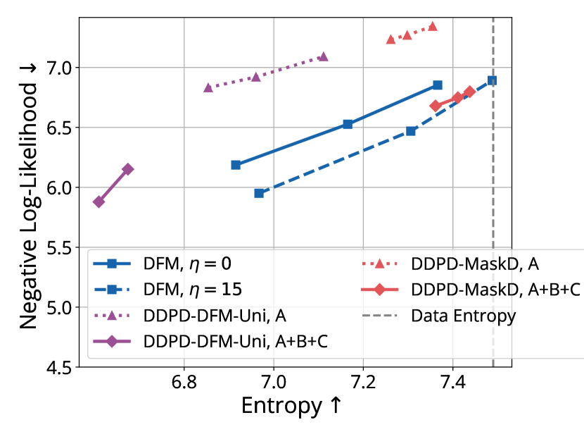
Figure 6: Comparing DDPD sampling under imperfect learning: 1) a single uniform diffusion model as planner + denoiser v.s. 2) separately trained planner + mask denoiser. The single uniform diffusion model converge slower in training and using DDPD sampler results in collapse in sample entropy. Using separate networks for planner and denoiser achieves results more close to SOTA methods in terms of quality v.s. diversity.

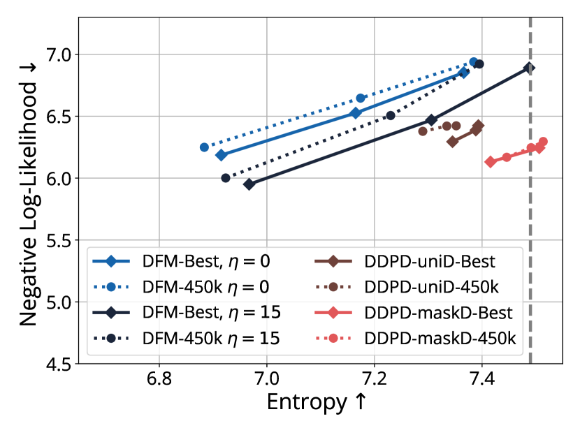
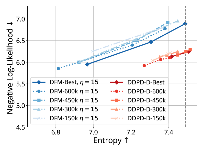
Figure 7: Left: Denoiser checkpoints at 450k v.s. 750k iterations. Right: Denoiser checkpoints at 150k, 300k, 450k, 600k, 750k iterations. DDPD is able to use an imperfect denoiser to achieve the same performance as the best possible.

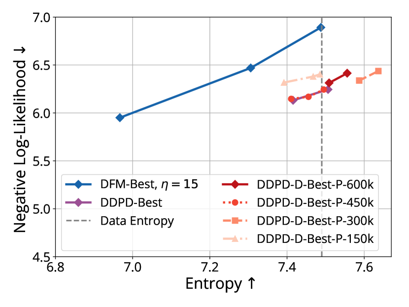
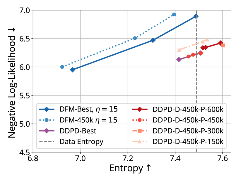
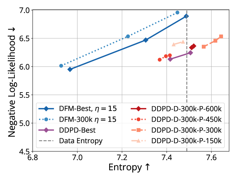
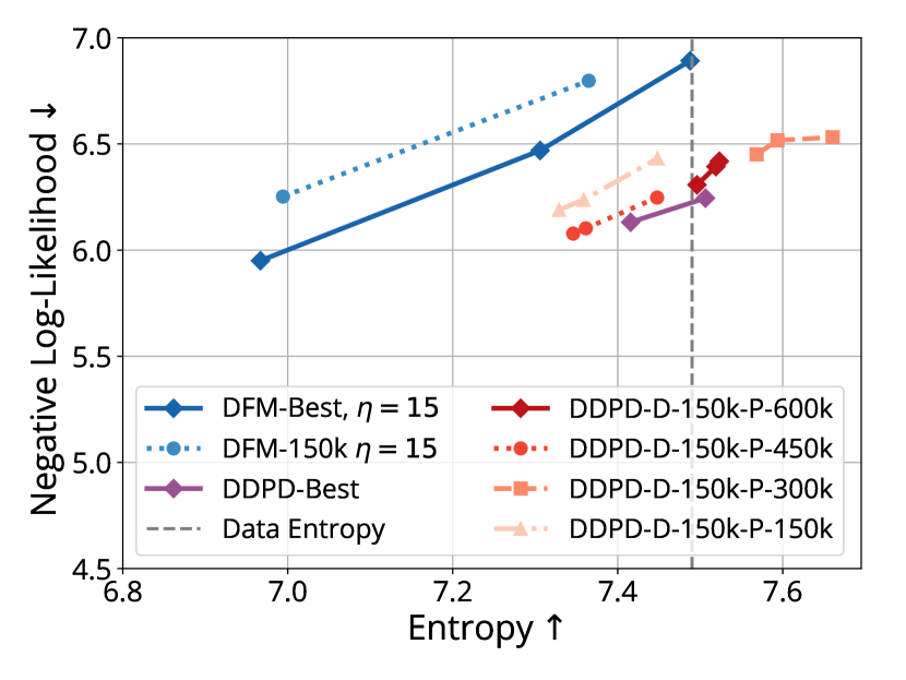
Figure 8: More ablation studies on pairing an imperfect denoiser with an imperfect planner.

E.1.2 Ablation of changes introduced in DDPD sampler

We conducted controlled experiment to measure the individual effect of the changes we introduced to the sampling process. Results are summarized in Fig. 9

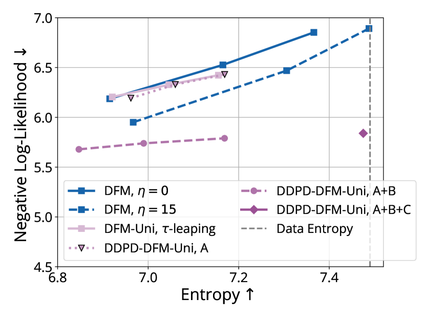
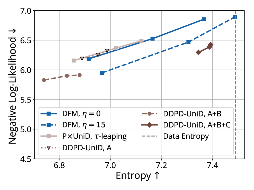
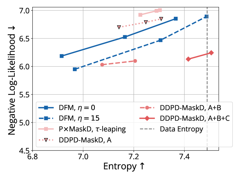
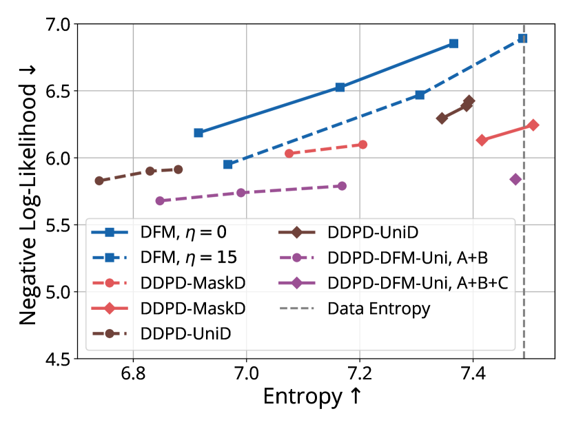
Figure 9: Ablation on introduced changes to discrete diffusion. A: Original Gillespie sampling. B: Time-adjustment based on the planner, continue sample until maximum number of steps is reached. C: Use $\text{softmax}(\texttt{logit\_if\_noise})$ instead of $\text{sigmoid}(\texttt{logit\_if\_noise})$ to pick which dimension to denoise next. The softmax trick makes the planning slightly more greedy than the original planning probability.

E.1.3 Model log-likelihoods on test data

Following ELBO terms derived in Section C.1, we calculate them for three different design choices:

• A single uniform diffusion neural network, but decomposed into planner and denoiser.

• Separate planner network and uniform diffusion denoiser network

• Separate planner network and mask diffusion denoiser network

In Table 4, we evaluate the ELBO terms for three methods both trained for $750k$ iterations (near optimality). We observe that the mask diffusoin denoiser has a better denonising performance even with mask approximation error introduced in the step of Proposition 3.5. In Table 5, We also observe mask diffusion denoiser performs better than uniform diffusion denoiser in terms the denoising log-likelihood.

Table 4: ELBO terms computed on the test set of text8 in bits-per-character (BPC) with fully trained models. Denoising likelihood only evaluates the probability of correctly denoising, for Planer + Mask Diffusion Denoiser, a mask is first sampled according to the planner.

Method	Rate Matching (BPC)	Transitioning (BPC)	Combined (BPC)
Uniform Diffusion	$\leq 0.0131$	$\leq 2.252$	$\leq 2.265$
Planner + Uniform Diffusion Denoiser	$\leq 0.0176$	$\leq 2.284$	$\leq 2.244$
Planner + Mask Diffusion Denoiser (given correct mask for denoising)	$\leq 0.0176$	$\leq 2.226$	$\leq 2.302$
Planner + Mask Diffusion Denoiser (use planner-predicted mask for denoising)	$\leq 0.0176$	$\leq 2.605$	$\leq 2.623$

Table 5: Denoising performance in bits-per-character (BPC). Mask Denoiser v.s. Uniform Diffusion Denoiser. Note that those are not entirely comparable as ELBO terms for uniform diffusion and mask diffusion are different.

Method	Denoising (BPC)	Denoising Accuracy at $\alpha_{t}=0.85$
Uniform Diffusion Denoiser	$\leq 2.063$	$92.2\%$
Mask Diffusion Denoiser	$\leq 1.367$	$96.8\%$

Table 6: ELBO terms computed on the test set of text8 in bits-per-character (BPC) with imperfect models trained at $20k$ iterations.

Method	Transitioning (BPC)	Combined (BPC)
Uniform Diffusion	$\leq 3.060$	$\leq 3.076$
Planner + Mask Diffusion Denoiser (given correct mask for denoising)	$\leq 2.854$	$\leq 2.843$
Planner + Mask Diffusion Denoiser (use planner-predicted mask for denoising)	$\leq 3.166$	$\leq 3.155$

E.2 OpenWebText

In Figs. 11 and 10, we measure generative perplexity of unconditional samples from GPT-2-small, GPT-2-medium, SEDD-small, SEDD-medium, DDPD-Small: Planner-small + SEDD-small-denoiser, DDPD-Medium: Planner-small + SEDD-small-denoiser. We also tested using $\text{sigmoid}(\texttt{logit\_if\_noise})$ and $\text{softmax}(\texttt{logit\_if\_noise})$ for planning. The difference is not as significant as in the text8 case. Using $\text{softmax}(\texttt{logit\_if\_noise})$ slightly increases entropy at the expense of perplexity. In Fig. 12, we find that DDPD using Planner-Small and SEDD-Denoiser-Small outperforms simply scaling up denoiser to SEDD-Medium.

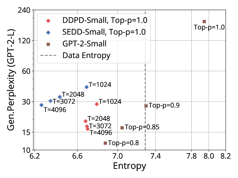
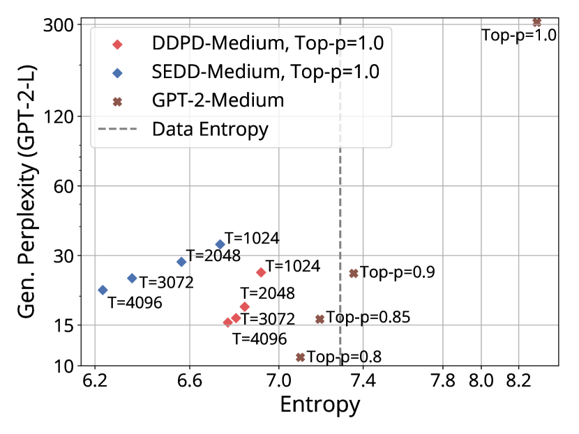
Figure 11: Using $\text{sigmoid}(\texttt{logit\_if\_noise})$ for planning. Generative perplexity evaluated with GPT-2 Large (GPT-2-L) and GPT-J: SEDD v.s. DDPD using the same denoiser.

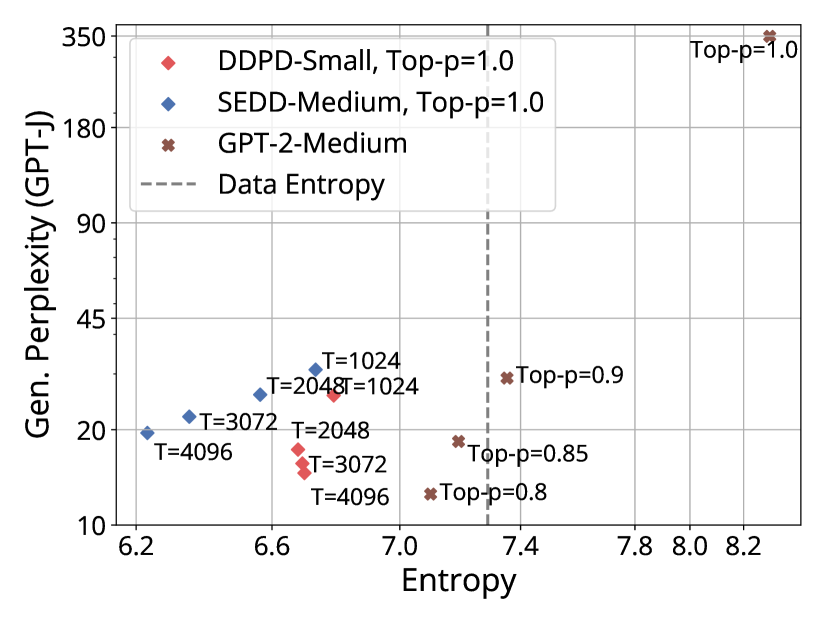
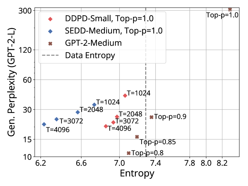
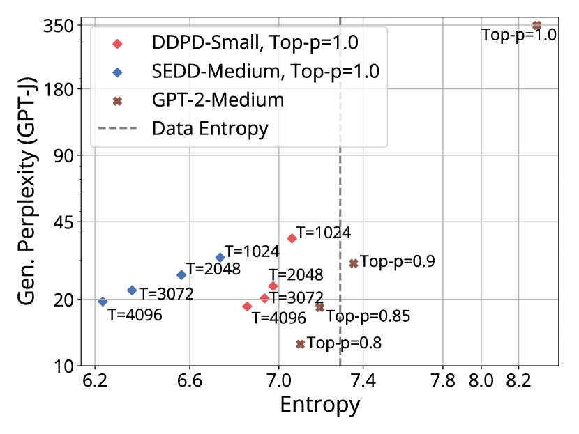
Figure 12: DDPD SEDD-small denoiser (90M) + Planner-small (90M) v.s. SEDD medium denoiser (320M) v.s. GPT-2-Medium (355M). DDPD with a smaller (less perfect) denoiser achieve better performance than simply using a larger (better) denoiser.

E.3 ImageNet $256\times 256$

Table 7: Inception Scores ($\uparrow$) on ImageNet $256\times 256$. MaskD refers to mask diffusion. The denoiser and parallel sampling schedule are kept the same as [45], without classifier-free guidance.

	No Logit Annealing			Logit temp $0.6$			Logit temp $1.0$ $\rightarrow$ $0.0$
Steps $T$	MaskD	MaskGIT	DDPD	MaskD	MaskGIT	DDPD	MaskD	MaskGIT	DDPD
$8$	33.56	199.83	149.98	149.28	271.73	201.67	157.19	249.86	213.03
$16$	39.36	248.88	178.17	179.85	281.73	173.48	164.01	263.47	185.25
$32$	43.30	266.17	169.49	200.33	281.36	156.22	170.73	268.88	158.14
$64$	45.06	274.56	160.74	206.06	281.14	146.27	171.62	269.45	145.95
$128$	45.56	276.45	152.61	210.27	278.88	138.55	142.40	272.73	137.19

Table 8: ImageNet $256\times 256$ generation results

Method	FID $\downarrow$	Inception Score $\uparrow$	Model size	$\#$ tokens	codebook
Taming-VQGAN [12]	15.78	78.3	1.4B	256	1024
RQ-VAE [23]	8.71	119.0	1.4B	256	16384
MaskGIT-VQGAN [8]	6.18	182.1	177M	256	1024
ViT-VQGAN [43]	4.17	175.1	1.7B	1024	8192
MAGVIT-v2 [44]	3.65	200.5	307M	2048	262144
1D-tokenizer [45] (annealing tricks)	4.61	166.7	287M	128	4096
DDPD-1D-tokenizer (w/o annealing tricks)	4.63	176.28	287M + 287M	128	4096

We study the effect of planned denoising with an increased number of refinement steps in Table 9. The FID first increases and then converges. The inception score also improves with increased refinement steps and then converges. From the visualized samples, we can see that plan-and-denoise sampling is very effective at fixing errors without losing its original content.

Table 9: FID Scores on ImageNet $256\times 256$. Increasing the number of refinement steps.

	Base steps $T=8$		Base steps $T=16$
Refinement Steps $T$	FID $\downarrow$	Inception Score $\uparrow$	FID $\downarrow$	Inception Score $\uparrow$
$8$	5.12	178.17	5.12	161.17
$16$	4.92	187.59	4.75	169.49
$32$	4.93	192.93	4.63	176.28
$48$	4.94	192.99	4.71	176.22

E.4 Noise estimation error using independent noise output $p_{\theta}(z_{t}^{d}|x_{t})$

We tested the assumption made in utilizing a pretrained mask diffusion denoiser by sampling joint noise latent variables using independent marginal prediction from a transformer for $p(z_{t}|x_{t},z_{t}^{d}=N)\approx\prod_{d^{\prime}\neq d}p_{\theta}(z_{t}^{d^{\prime}}|x_{t})$ in Table 10. We observe that the assumption holds almost perfectly in language modeling such as OpenWebText. On character modeling task text8, the assumption also holds most of the time, especially near the end of generation, but it is more complicated than word tokens due to a much smaller vocabulary. This is also discovered in Table 4 where we observe the two-step sampling introduces approximation errors and hence makes the log-likelihood for denoising lower.

Table 10: Accuracy on Mask Prediction for text8 and OpenWebText at fixed times. Mask accuracy measures if the independent sampling matches the joint noise variable values. Almost deterministic measures the assumption $p(z_{t}^{\bar{d}}|x_{t},z_{t}^{d}=N)\approx 1$. We set the threshold to be $\mathrm{logit.abs()}>3.0$.

Fixed Time	text8		OpenWebText
$t=1\rightarrow 0$	Mask Accuracy	If Deterministic	Mask Accuracy	If Deterministic
(Data) 1.0	0.9988	0.9975	0.9999	0.9997
0.95	0.9915	0.9864	0.9985	0.9960
0.8	0.9623	0.9238	0.9943	0.9851
0.6	0.8784	0.6789	0.9847	0.9585
0.4	0.7416	0.2261	0.9679	0.9100
0.2	0.7402	0.2125	0.9476	0.8466
0.05	0.8878	0.4800	0.9599	0.8817
(Noise) 0.0	0.9465	0.5974	0.9975	0.9906

Appendix F Generation examples

F.1 Generated samples from models trained on text8

We compare samples between DFM and DDPD. For DDPD, we include samples from three models: 1) DDPD-DFM-Uni: planner and denoiser from a single uniform diffusion denoiser model $p_{1|t}^{\theta}(x_{1}^{d}|x_{t})$ using Eq. 10 and Eq. 11; 2) DDPD-UniD: a planner network $p(z_{t}^{d}|x_{t})$ and a uniform diffusion denoiser network $p_{1|t}(x_{1}^{d}|x_{t},z_{t}^{d}=N)$; 3) DDPD-MaskD: a planner network $p(z_{t}^{d}|x_{t})$ and a mask diffusion denoiser network $p_{1|t}(x_{1}^{d}|x_{t},z_{t}^{d}=N)$.

F.2 Generated samples from models trained on OpenWebText

In general, samples from DDPD demonstrate a better ability to capture word correlations, leading to greater coherence compared to those generated by SEDD. However, both methods exhibit less coherence in longer contexts when compared to samples from GPT-2 models.

F.3 Generated samples from models trained on ImageNet $256\times 256$

In Figs. 14, 15 and 16, we visualize samples of DDPD, Mask Diffusion and MaskGIT.

Without logit temperature annealing, Mask Diffusion captures diversity, but the sample quality suffers due to imperfections in the denoiser. On the other hand, MaskGIT’s confidence-based strategy significantly improves sample quality, but at the cost of reduced diversity. DDPD trades off diversity v.s. quality naturally without the need for any annealing or confidence-based tricks.

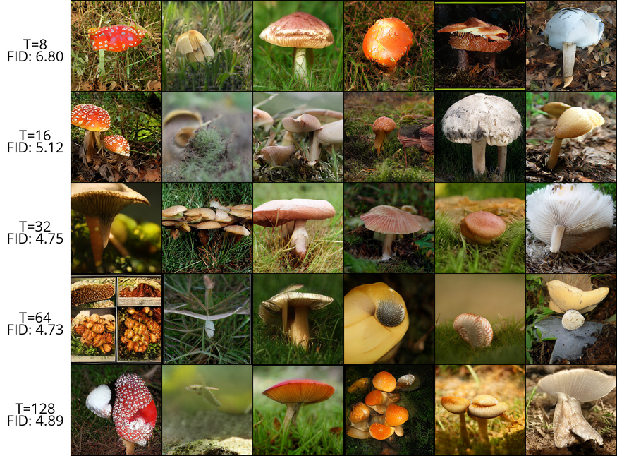
(a) DDPD: No Annealing

(b) Mask Diffusion: No Annealing

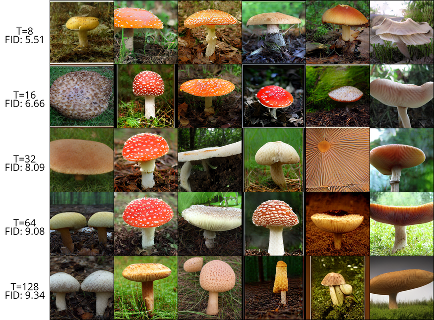
(c) MaskGIT: No Annealing

Figure 14: DDPD v.s. Mask Diffusion v.s. MaskGIT, No Logit Annealing

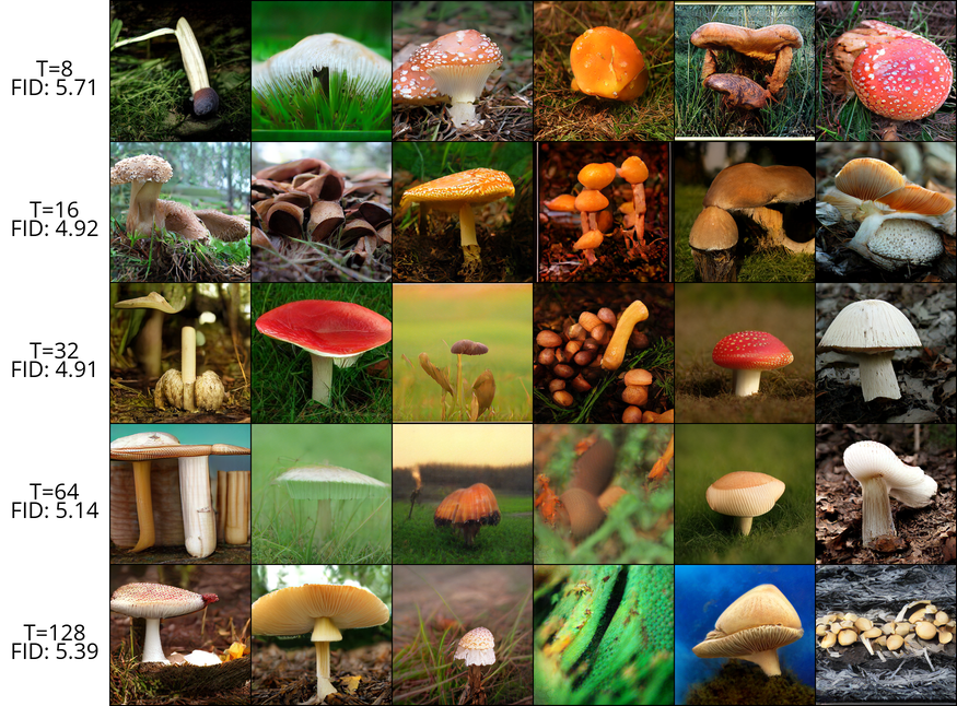
(a) DDPD: Logit Annealing $=0.6$

(b) Mask Diffusion: Logit Annealing $=0.6$

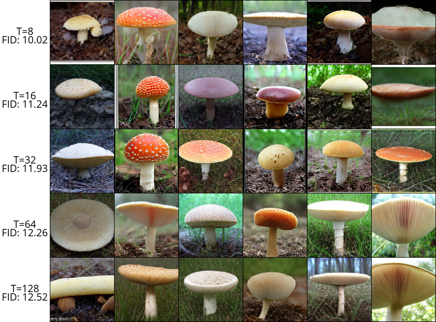
(c) MaskGIT: No Logit Annealing $1.0\rightarrow 0.0$

Figure 15: DDPD v.s. Mask Diffusion v.s. MaskGIT, Logit Annealing $=0.6$

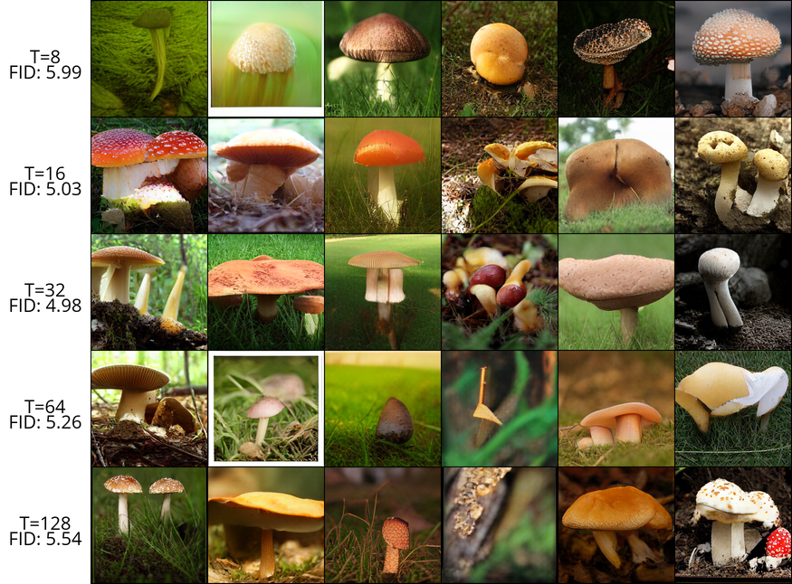
(a) DDPD: Logit Annealing $1.0\rightarrow 0.0$

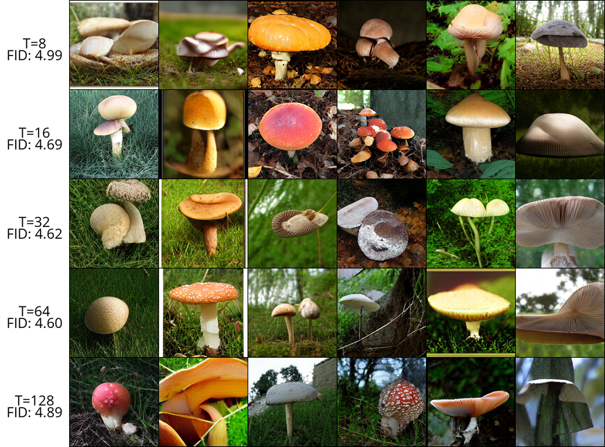
(b) Mask Diffusion: Logit Annealing $1.0\rightarrow 0.0$

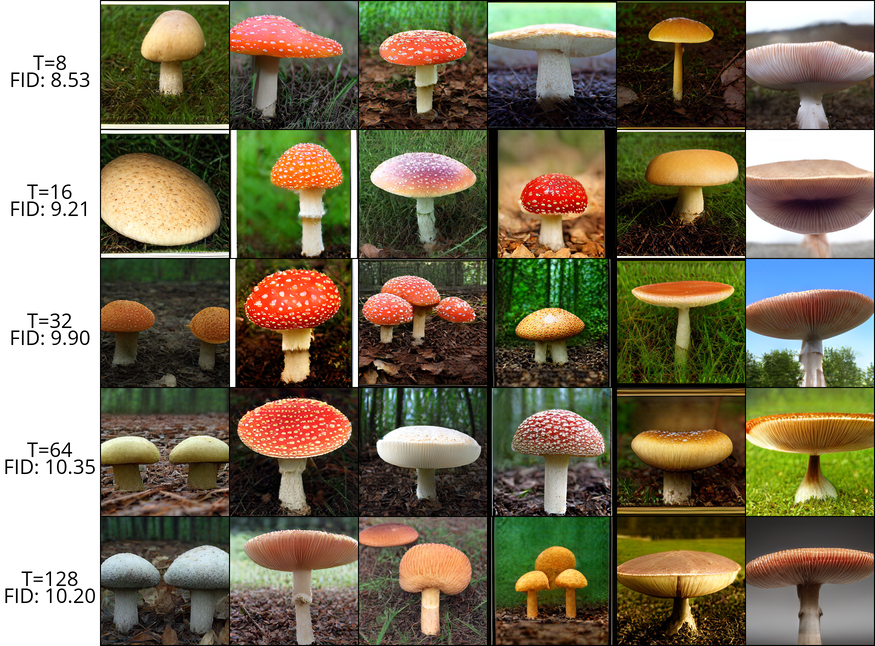
(c) MaskGIT: Logit Annealing $1.0\rightarrow 0.0$

Figure 16: DDPD v.s. Mask Diffusion v.s. MaskGIT, Logit Annealing $1.0\rightarrow 0.0$

(a) DDPD $32$ steps

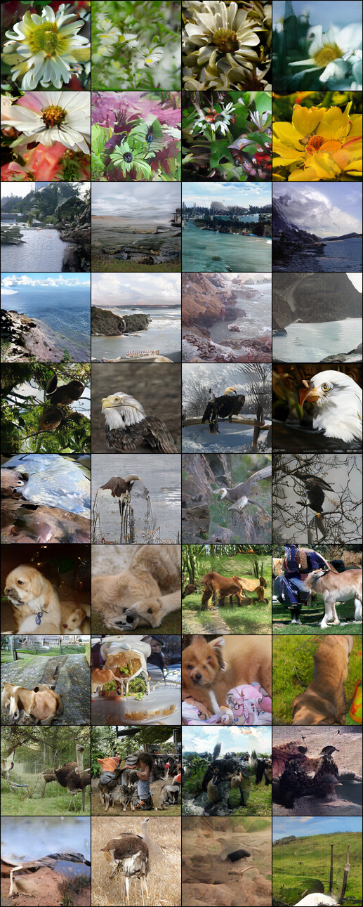
(b) Mask Diffusion $32$ steps

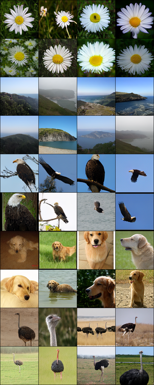
(c) MaskGIT $32$ steps

Figure 17: DDPD v.s. Mask Diffusion v.s. MaskGIT, No Logit Annealing

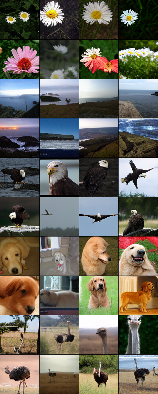
(a) DDPD $32$ steps

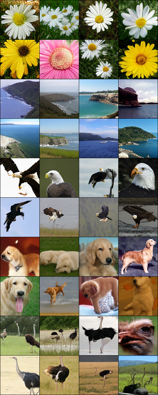
(b) Mask Diffusion $32$ steps

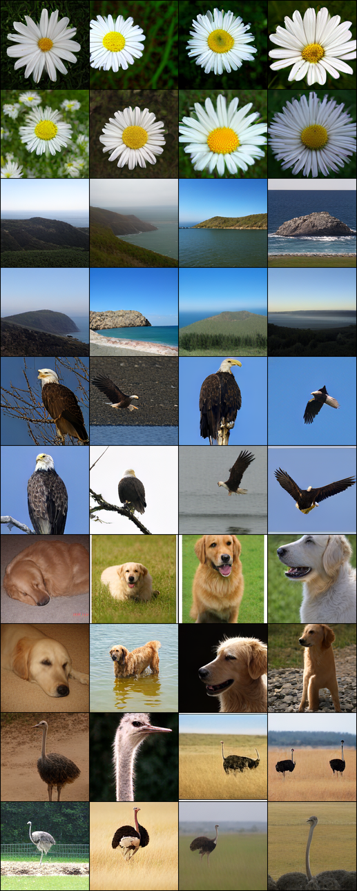
(c) MaskGIT $32$ steps

Figure 18: DDPD v.s. Mask Diffusion v.s. MaskGIT, Logit Annealing $1.0\rightarrow 0.0$

(a) DDPD $16+16$ steps

(b) DDPD $16+32$ steps

Figure 19: DDPD No Annealing, increasing number of refinement steps. The added refinement steps act as “touch-up” to improve the aesthetic quality without losing its original content.

Appendix G Reproducibility statement

To facilitate reproducibility, we provide comprehensive details of our method in the main paper and Appendix D. This includes the model designs, hyper-parameters in training, sampling schemes and evaluation protocols for all the experiments. We further provide PyTorch pseudocode for the proposed adaptive Gillespie sampling algorithm.

Appendix H Ethics Statement

This work raises ethical considerations common to deep generative models. While offering potential benefits such as generating high-quality text/image contents, these models can also be misused for malicious purposes like creating deepfakes or generating spam and misinformation. Mitigating these risks requires further research into guardrails for reducing harmful contents and collaboration with socio-technical experts.

Furthermore, the substantial resource costs associated with training and deploying deep generative models, including energy and water consumption, present environmental concerns. This work is able save cost on training by reusing a pretrained denoisers and just focusing on training different planner models for slightly different tasks. At inference time, our newly proposed sampler is able to generate at better quality as compared to existing methods that use same amount of compute.

References

- Alamdari et al. [2023] Sarah Alamdari, Nitya Thakkar, Rianne van den Berg, Alex X Lu, Nicolo Fusi, Ava P Amini, and Kevin K Yang. Protein generation with evolutionary diffusion: sequence is all you need. BioRxiv, pp. 2023–09, 2023.
- Albergo & Vanden-Eijnden [2023] Michael S Albergo and Eric Vanden-Eijnden. Building normalizing flows with stochastic interpolants. International Conference on Learning Representations, 2023.
- Austin et al. [2021] Jacob Austin, Daniel D Johnson, Jonathan Ho, Daniel Tarlow, and Rianne Van Den Berg. Structured denoising diffusion models in discrete state-spaces. Advances in Neural Information Processing Systems, 2021.
- Avdeyev et al. [2023] Pavel Avdeyev, Chenlai Shi, Yuhao Tan, Kseniia Dudnyk, and Jian Zhou. Dirichlet diffusion score model for biological sequence generation. In International Conference on Machine Learning, 2023.
- Brown et al. [2020] Tom B Brown, Benjamin Mann, Nick Ryder, Melanie Subbiah, Jared Kaplan, Prafulla Dhariwal, Arvind Neelakantan, Pranav Shyam, Girish Sastry, Amanda Askell, et al. Language models are few-shot learners. In Advances in neural information processing systems, 2020.
- Campbell et al. [2022] Andrew Campbell, Joe Benton, Valentin De Bortoli, Thomas Rainforth, George Deligiannidis, and Arnaud Doucet. A continuous time framework for discrete denoising models. Advances in Neural Information Processing Systems, 2022.
- Campbell et al. [2024] Andrew Campbell, Jason Yim, Regina Barzilay, Tom Rainforth, and Tommi Jaakkola. Generative flows on discrete state-spaces: Enabling multimodal flows with applications to protein co-design. International Conference on Machine Learning, 2024.
- Chang et al. [2022] Huiwen Chang, Han Zhang, Lu Jiang, Ce Liu, and William T Freeman. Maskgit: Masked generative image transformer. In Proceedings of the IEEE/CVF Conference on Computer Vision and Pattern Recognition, pp. 11315–11325, 2022.
- Chang et al. [2023] Huiwen Chang, Han Zhang, Jarred Barber, Aaron Maschinot, Jose Lezama, Lu Jiang, Ming-Hsuan Yang, Kevin Patrick Murphy, William T Freeman, Michael Rubinstein, et al. Muse: Text-to-image generation via masked generative transformers. In International Conference on Machine Learning, 2023.
- Chen et al. [2023] Zixiang Chen, Huizhuo Yuan, Yongqian Li, Yiwen Kou, Junkai Zhang, and Quanquan Gu. Fast sampling via de-randomization for discrete diffusion models. arXiv preprint arXiv:2312.09193, 2023.
- Dhariwal & Nichol [2021] Prafulla Dhariwal and Alexander Nichol. Diffusion models beat gans on image synthesis. Advances in neural information processing systems, 34:8780–8794, 2021.
- Esser et al. [2021] Patrick Esser, Robin Rombach, and Björn Ommer. Taming transformers for high-resolution image synthesis. In Proceedings of the IEEE/CVF Conference on Computer Vision and Pattern Recognition (CVPR), pp. 12873–12883, 2021.
- Gat et al. [2024] Itai Gat, Tal Remez, Neta Shaul, Felix Kreuk, Ricky TQ Chen, Gabriel Synnaeve, Yossi Adi, and Yaron Lipman. Discrete flow matching. arXiv preprint arXiv:2407.15595, 2024.
- Ghazvininejad et al. [2019] Marjan Ghazvininejad, Omer Levy, Yinhan Liu, and Luke Zettlemoyer. Mask-predict: Parallel decoding of conditional masked language models. In EMNLP-IJCNLP, 2019.
- Gillespie [1976] Daniel T Gillespie. A general method for numerically simulating the stochastic time evolution of coupled chemical reactions. Journal of computational physics, 22(4):403–434, 1976.
- Gillespie [1977] Daniel T Gillespie. Exact stochastic simulation of coupled chemical reactions. The journal of physical chemistry, 81(25):2340–2361, 1977.
- Gokaslan & Cohen [2019a] A. Gokaslan and V. Cohen. Openwebtext corpus. http://Skylion007.github.io/OpenWebTextCorpus, 2019a.
- Gokaslan & Cohen [2019b] Aaron Gokaslan and Vanya Cohen. OpenWebText Corpus, 2019b. URL http://Skylion007.github.io/OpenWebTextCorpus.
- Heusel et al. [2017] Martin Heusel, Hubert Ramsauer, Thomas Unterthiner, Bernhard Nessler, and Sepp Hochreiter. GANs trained by a two time-scale update rule converge to a local Nash equilibrium. Advances in neural information processing systems, 30, 2017.
- Holtzman et al. [2019] Ari Holtzman, Jan Buys, Li Du, Maxwell Forbes, and Yejin Choi. The curious case of neural text degeneration. In International Conference on Learning Representations, 2019.
- Hoogeboom et al. [2021] Emiel Hoogeboom, Didrik Nielsen, Priyank Jaini, Patrick Forré, and Max Welling. Argmax flows and multinomial diffusion: Learning categorical distributions. Advances in Neural Information Processing Systems, 34:12454–12465, 2021.
- Karras et al. [2022] Tero Karras, Miika Aittala, Timo Aila, and Samuli Laine. Elucidating the design space of diffusion-based generative models. Advances in neural information processing systems, 2022.
- Lee et al. [2022a] Doyup Lee, Chiheon Kim, Saehoon Kim, Minsu Cho, and Wook-Shin Han. Autoregressive image generation using residual quantization. In Proceedings of the IEEE/CVF Conference on Computer Vision and Pattern Recognition (CVPR), pp. 11452–11461, 2022a.
- Lee et al. [2022b] Doyup Lee, Chiheon Kim, Saehoon Kim, Minsu Cho, and WOOK SHIN HAN. Draft-and-revise: Effective image generation with contextual rq-transformer. Advances in Neural Information Processing Systems, 35:30127–30138, 2022b.
- Lin et al. [2023] Zeming Lin, Halil Akin, Roshan Rao, Brian Hie, Zhongkai Zhu, Wenting Lu, Nikita Smetanin, Robert Verkuil, Ori Kabeli, Yaniv Shmueli, et al. Evolutionary-scale prediction of atomic-level protein structure with a language model. Science, 379(6637):1123–1130, 2023.
- Lipman et al. [2023] Yaron Lipman, Ricky TQ Chen, Heli Ben-Hamu, Maximilian Nickel, and Matt Le. Flow matching for generative modeling. International Conference on Learning Representations, 2023.
- Liu et al. [2023] Xingchao Liu, Chengyue Gong, and Qiang Liu. Flow straight and fast: Learning to generate and transfer data with rectified flow. International Conference on Learning Representations, 2023.
- Loshchilov & Hutter [2019] Ilya Loshchilov and Frank Hutter. Decoupled weight decay regularization. arXiv preprint arXiv:1711.05101, 2019.
- Lou et al. [2024] Aaron Lou, Chenlin Meng, and Stefano Ermon. Discrete diffusion language modeling by estimating the ratios of the data distribution. International Conference on Machine Learning, 2024.
- Mahoney [2011] Matt Mahoney. Large text compression benchmark, 2011. URL http://mattmahoney.net/dc/textdata.html.
- Norris [1998] James R Norris. Markov chains. Number 2. Cambridge university press, 1998.
- Peebles & Xie [2023] William Peebles and Saining Xie. Scalable diffusion models with transformers, 2023.
- Radford et al. [2019] Alec Radford, Jeffrey Wu, Rewon Child, David Luan, Dario Amodei, Ilya Sutskever, et al. Language models are unsupervised multitask learners. OpenAI blog, 1(8):9, 2019.
- Sahoo et al. [2024] Subham Sekhar Sahoo, Marianne Arriola, Yair Schiff, Aaron Gokaslan, Edgar Marroquin, Justin T Chiu, Alexander Rush, and Volodymyr Kuleshov. Simple and effective masked diffusion language models. arXiv preprint arXiv:2406.07524, 2024.
- Savinov et al. [2022] Nikolay Savinov, Junyoung Chung, Mikolaj Binkowski, Erich Elsen, and Aaron van den Oord. Step-unrolled denoising autoencoders for text generation. In International Conference on Learning Representations, 2022.
- Shi et al. [2024] Jiaxin Shi, Kehang Han, Zhe Wang, Arnaud Doucet, and Michalis K Titsias. Simplified and generalized masked diffusion for discrete data. arXiv preprint arXiv:2406.04329, 2024.
- Song et al. [2020] Yang Song, Jascha Sohl-Dickstein, Diederik P Kingma, Abhishek Kumar, Stefano Ermon, and Ben Poole. Score-based generative modeling through stochastic differential equations. International Conference on Learning Representations, 2020.
- Su et al. [2024] Jianlin Su, Murtadha Ahmed, Yu Lu, Shengfeng Pan, Wen Bo, and Yunfeng Liu. Roformer: Enhanced transformer with rotary position embedding. Neurocomputing, 568:127063, 2024.
- Sun et al. [2023] Haoran Sun, Lijun Yu, Bo Dai, Dale Schuurmans, and Hanjun Dai. Score-based continuous-time discrete diffusion models. International Conference on Learning Representations, 2023.
- Wang & Komatsuzaki [2021] Ben Wang and Aran Komatsuzaki. GPT-J-6B: A 6 billion parameter autoregressive language model, 2021. URL https://github.com/kingoflolz/mesh-transformer-jax.
- Wilkinson [2018] Darren J Wilkinson. Stochastic modelling for systems biology. Chapman and Hall/CRC, 2018.
- Xu et al. [2023] Yilun Xu, Mingyang Deng, Xiang Cheng, Yonglong Tian, Ziming Liu, and Tommi Jaakkola. Restart sampling for improving generative processes. Advances in Neural Information Processing Systems, 36:76806–76838, 2023.
- Yu et al. [2022] Jiahui Yu, Xin Li, Jing Yu Koh, Han Zhang, Ruoming Pang, James Qin, Alexander Ku, Yuanzhong Xu, Jason Baldridge, and Yonghui Wu. Vector-quantized image modeling with improved vqgan. In International Conference on Learning Representations (ICLR), 2022.
- Yu et al. [2024a] Lijun Yu, José Lezama, Nitesh B Gundavarapu, Luca Versari, Kihyuk Sohn, David Minnen, Yong Cheng, Agrim Gupta, Xiuye Gu, Alexander G Hauptmann, et al. Language model beats diffusion–tokenizer is key to visual generation. In International Conference on Learning Representations (ICLR), 2024a.
- Yu et al. [2024b] Qihang Yu, Mark Weber, Xueqing Deng, Xiaohui Shen, Daniel Cremers, and Liang-Chieh Chen. An image is worth 32 tokens for reconstruction and generation. arXiv preprint arXiv:2406.07550, 2024b.
- Zheng et al. [2023] Lin Zheng, Jianbo Yuan, Lei Yu, and Lingpeng Kong. A reparameterized discrete diffusion model for text generation. arXiv preprint arXiv:2302.05737, 2023.