On the impact of neutrinos on the launching of relativistic jets from “magnetars” produced in neutron-star mergers

Abstract

A significant interest has emerged recently in assessing whether collimated and ultra-relativistic outflows can be produced by a long-lived remnant from a binary neutron-star (BNS) merger, with different approaches leading to different outcomes. To clarify some of the aspect of this process, we report the results of long-term (i.e., $\sim~{}110\,{\rm ms}$) state-of-the-art general-relativistic magnetohydrodynamics simulations of the inspiral and merger of a BNS system of magnetized stars. We find that after $\sim~{}50\,{\rm ms}$ from the merger, an $\alpha$-$\Omega$ dynamo driven by the magnetorotational instability (MRI) sets-in in the densest regions of the disk and leads to the breakout of the magnetic-field lines from the accretion disk around the remnant. The breakout, which can be associated with the violation of the Parker-stability criterion, is responsible for the generation of a collimated, magnetically-driven outflow with only mildly relativistic velocities that is responsible for a violent eruption of electromagnetic energy. We provide evidence that this outflow is partly collimated via a Blandford-Payne mechanism driven by the open field lines anchored in the inner disk regions. Finally, by including or not the radiative transport via neutrinos, we determine the role they play in the launching of the collimated wind. In this way, we conclude that the mechanism of magnetic-field breakout we observe is robust and takes place even without neutrinos. Contrary to previous expectations, the inclusion of neutrinos absorption and emission leads to a smaller baryon pollution in polar regions, and hence accelerates the occurrence of the breakout, yielding a larger electromagnetic luminosity. Given the mildly relativistic nature of these disk-driven breakout outflows, it is difficult to consider them responsible for the jet phenomenology observed in short gamma-ray bursts.

1 Introduction

Binary neutron star (BNS) mergers are known to be the progenitors of transient electromagnetic (EM) emission phenomena such as kilonovae and short gamma-ray bursts. The mass distribution of pulsars in galactic binaries, combined with estimates on the maximum mass that can be supported against gravitational collapse by the equation of state (EOS), and the results of numerical-relativity simulations, suggest that the outcome of a typical merger of two neutron stars is a differentially rotating hypermassive neutron star (HMNS), which survives for a timescale on the order of $\sim~{}100\,{\rm ms}$ to $\sim~{}1\,{\rm s}$ before collapsing to form a black hole (see, e.g.,  Baiotti & Rezzolla, 2017; Paschalidis, 2017, for some reviews). This timescale is also relevant for the development of the EM counterparts to BNS mergers, as testified by the GW170817 event (Abbott et al., 2017), where a delay of $\sim~{}1.7\,{\rm s}$ was measured between the EM and the gravitational-wave (GW) signal. This time is normally associated to the survival of the HMNS and the launching of a highly relativistic collimated jet, which successfully broke out of the ejected material surrounding the central engine (Gill et al., 2019; Murguia-Berthier et al., 2016, 2021), see also Metzger & Fernández (2014) for additional constraints from changes in the afterglow.

Since the launching of such a jet is likely to require an ordered and large-scale magnetic field, it is important to study in detail whether and how such a structure can emerge in the presence of a magnetized HMNS, or “magnetar”. Moreover, the massive blue kilonova that was also observed following GW170817 implies that a large quantity of high electron-fraction material, i.e., with $Y_{e}>0.25$, was ejected at mildly relativistic speeds by the merger remnant. Since the progenitors in the BNS system are initially very neutron rich, this material can only be explained by the re-processing of the ejecta by weak interactions and hence the irradiation of neutrinos (Metzger & Fernández, 2014). Furthermore, because the disk around the black hole formed after merger is unlikely to reach temperatures and densities high enough to emit a sufficient amount of electron anti-neutrinos, a long-lived HMNS remnant is probably the only viable explanation to the blue-kilonova mass observed in GW170817. Clearly, a detailed understanding of the evolution of a magnetized HMNS on secular timescales is essential for the modelling of the EM counterparts of BNS mergers in general, and for the launching of collimated outflows from metastable BNS merger remnants, in particular.

A recent study based on long-term, numerical-relativity simulation of black-hole–neutron-star mergers (Gottlieb et al., 2023a) suggests that while a sub-population of compact merger long gamma-ray bursts are likely powered by black holes surrounded by an accretion disk, short gamma-ray bursts may be better explained by magnetar engines (Gottlieb et al., 2023b). However, direct ab-initio numerical evidence of whether a HMNS can power a gamma-ray burst remains inconclusive (see, e.g.,  Ciolfi, 2020; Mösta et al., 2020; Most & Quataert, 2023; Combi & Siegel, 2023; Kiuchi et al., 2024; Bamber et al., 2024; Aguilera-Miret et al., 2024). This is due, in great part, to the significant challenges involved with simulating a differentially rotating HMNS remnant at a sufficiently high resolution and over a sufficiently long timescale to be able to track the evolution of the topology and strength of the magnetic field.

By employing ultra-high resolutions, a recent work (Kiuchi et al., 2024) has also highlighted how a magneto-rotational instability (MRI) driven $\alpha$-$\Omega$ dynamo (Ruediger & Kichatinov, 1993; Bonanno et al., 2003), might be at play in the outer layers of the remnant, which might ultimately lead to breakout of the magnetic field from the surface of the star and to a magnetically driven collimated outflow. These direct simulations have been followed by other studies that have tried to reproduce the effect of an $\alpha$-$\Omega$ dynamo in simulations by incorporating effective dynamo terms in the equations themselves (Most, 2023). An important caveat in this process is the impact of neutrino-driven winds from the stellar surface, which are expected to lower the Lorentz factor reached in these outflows (Dessart et al., 2009).

The study presented here is meant to address and hopefully shed light on a number of the open questions discussed above. In particular, we focus on the impact of neutrinos on the outflows and present a launching mechanism driven by buoyant magnetic field breakout from the remnant accretion disk. To this end, we perform long-term and full general-relativistic magnetohydrodynamics (GRMHD) evolutions of the inspiral and merger of a binary system of magnetized neutron stars with a full moment-based treatment of neutrinos. We find that contrary to previous expectations, the inclusion of neutrinos do not lead to additional baryon pollution of the outflows, nor do they inhibit magnetic field breakout, but speed-up this process compared to a scenario where they are not included.

2 Methods

We perform our simulations within the ideal-GRMHD approximation (see, e.g.,  Mizuno & Rezzolla, 2024, for a recent review) with adaptive-mesh-refinement (AMR) provided by the EinsteinToolkit (Haas & et al., 2020). The GRMHD equations are solved with fourth-order accurate finite differences by the Frankfurt/IllinoisGRMHD (FIL) code (Most et al., 2019; Etienne et al., 2015) and the divergence-free constraint of the magnetic field is ensured via constrained transport evolution of the magnetic vector potential (Londrillo & Del Zanna, 2004) (see also Etienne et al. (2010, 2012)). FIL provides its own spacetime evolution code based on the Z4c system (Hilditch et al., 2013), as well as a framework for handling temperature and composition-dependent equations of state (EOSs) (Most et al., 2019, 2020). Neutrinos are accounted for through the energy-integrated, moment-based M1 scheme FIL-M1 (see Musolino & Rezzolla, 2024, for details on our implementation), which self-consistently accounts for energy and momentum transfers between neutrinos and the astrophysical plasma as well as for composition changes in the fluid due to weak processes. In order to investigate the impact of dynamo processes in the disk unambiguously, we do not employ the mean-field dynamo module available in FIL (Most, 2023). Last but not least, high quality initial data for our binaries is obtained with the FUKA solver Papenfort et al. (2021); Tootle (2024).

Using this computational infrastructure, we have performed two long-term, i.e., $\gtrsim 110\,{\rm ms}$, simulations of equal-mass BNS mergers described by the BHB$\Lambda\phi$ EOS (Banik et al., 2014), where each of the star has an isolated ADM mass of $M_{\rm ADM}=1.25\,M_{\odot}$. This value is chosen as to ensure that the HMNS is metastable over a timescale of a few $100\,{\rm ms}$ before collapsing to form a black hole. We perform our simulations on a fixed mesh-refinement (FMR) grid with eight levels, where the finest one has a spacing of $dx_{\rm f}\sim 210\,{\rm m}$ and covers a volume of $[-70,70]^{2}\times[0,35]\,{\rm km}$ to ensure that the HMNS and the densest regions of the disk are contained within the finest refinement level. The entire domain covers $\sim[-10^{4},10^{4}]^{2}\times[0,10^{4}]\,{\rm km}$ and we employ $z$-reflection symmetry to save computational costs.

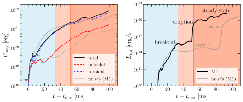
Figure 1: Left panel: Evolution of the total magnetic energy (black solid line) but also of the poloidal (red dashed line) and toroidal components (blue dotted line). Also shown with gray lines of the same type are the corresponding evolutions when no neutrinos are taken into account (no ${\rm M1}$). Right panel: Evolution of the EM luminosity during the simulation. Note the large jump when the magnetically-driven wind, that is emitted at the “breakout” reaches the detector at the “eruption” time and is sustained in a steady state. Shown with gray lines is the luminosity in the absence of neutrinos (no ${\rm M1}$) and highlighting that neutrinos are useful to trigger the breakout but not necessary.

The magnetic field is initially confined to the stars and is initialised so that the maximum magnetic-field strength is $B_{0}=10^{16.5}\,{\rm G}$ (see Chabanov et al., 2023, for more details). We caution that our choice of spatial resolutions – dictated by the of acceptable computational costs over the long timescales considered here – is insufficient to capture all aspects of magnetic field amplification associated with the MRI-driven dynamo, which especially inside the outer layers of the HMNS have been shown to require at least $70\,\rm m$ (Kiuchi et al., 2018). However, the mechanism presented in this work only relies on dynamo processes in the accretion disk, which are fully captured at this resolution. In addition, the extremely large value of the magnetic field is chosen to be able to resolve at least partially the MRI in the inner layers of the disk after merger. Finally, to assess the role neutrinos play in the breakout of the magnetic field, and the baryon pollution of polar outflows, we perform two sets of simulations with and without the inclusion of neutrinos vi an M1 scheme. This choice doubles our computational costs but, as we will discuss, provides precious information.

3 Results

3.1 Magnetic evolution and observables

Because much of our focus here is on the long-term post-merger dynamics of the remnant, we will not discuss in detail the main aspects of the inspiral of magnetized binaries, which have been presented in several works before (see, e.g.,  Liu et al., 2008; Giacomazzo et al., 2009; Palenzuela et al., 2015, for some early investigations). Similarly, we will not present the complex dynamics that takes place at the merger and though the development of the KHI and that has also been discussed in a number of publications over the years (see, e.g.,  Price & Rosswog, 2006; Giacomazzo et al., 2011; Kiuchi et al., 2015a; Aguilera-Miret et al., 2020; Chabanov et al., 2023, for some early and recent works). Hence, our discussion will be restricted to the post-merger remnant starting from a timescale of few tens of milliseconds after the merger. At this point, the HMNS has reached a quasi-stationary equilibrium that is essentially axisymmetric but for the presence of small non-axisymmetric perturbations – quantifiable mostly in the $m=1$ and $m=2$ modes (see, e.g.,  Lehner et al., 2016; Radice et al., 2016; East et al., 2019; Papenfort et al., 2022; Topolski et al., 2024) – and in a differential-rotation profile characterized by a slowly uniformly rotating core and a Keplerian mantle or “disk” (Kastaun & Galeazzi, 2015; Hanauske et al., 2017; Uryū et al., 2017; Cassing & Rezzolla, 2024).

Under these conditions, turbulence in the remnant is fully developed (with properties that depend on resolution Aguilera-Miret et al. (2022); Palenzuela et al. (2022); Chabanov & Rezzolla (2023)) and more stationary, so that large-scale shearing motions can be produced and lead to the so-called “magnetic-winding”. We recall that, under the infinite-conductivity conditions of ideal MHD, coherent large-scale shearing motions lead a growth of the magnetic-field strength that is linear in time (Liu & Shapiro, 2004). Obviously, as kinetic energy is progressively transformed into magnetic energy, the winding stage cannot continue indefinitely and is expected to terminate when the magnetic-field energy is in rough equipartition with the kinetic energy stored in the differential rotation, so that further amplification is energetically disfavoured. All of this can be directly deduced from the left panel of Fig. 1, which reports the evolution of the total magnetic energy (black solid line) and of its poloidal (red dashed line) and toroidal (blue dotted line) components. Note that the KHI takes place at merger and leads to an exponential growth of the toroidal and poloidal components for $t-t_{\rm mer}\lesssim 5\,{\rm ms}$. After the KHI is quenched and the merger has taken place, the poloidal component essentially stops growing, while the toroidal component – which was absent before merger – becomes the dominant component (see, e.g.,  Kiuchi et al., 2015b; Palenzuela et al., 2022; Chabanov et al., 2023, for a detailed discussion of the magnetic-field evolution soon after the merger). It is worth noting that the initial magnetic-field strength in our simulations is considerably stronger than what is expected for old magnetized neutron stars in a merger process. This has been shown to impact the topology of the field after the initial amplification phase is terminated (Aguilera-Miret et al., 2024).

While these dynamics largely concern the magnetic field inside the high-density region of the HMNS, the accretion-disk dynamics and dynamo inside the disk will largely be governed by the MRI and shear-current effects (Christie et al., 2019; Liska et al., 2018; Jacquemin-Ide et al., 2024). It is this dynamics that leads to the growth of the poloidal component and to a subsequent breakout as the one we will describe below.

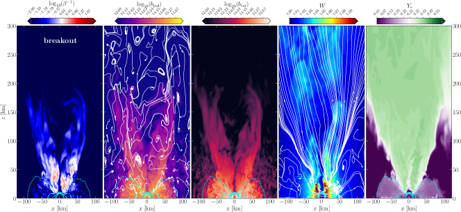
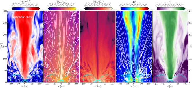
Figure 2: Two-dimensional distributions in the $(x,z)$ plane of various quantities computed in the simulations. Starting from the left, we report: the inverse plasma-$\beta$, i.e., the ratio of the magnetic to thermal pressures the poloidal, $b_{\rm pol}$, and toroidal, $b_{\rm tor}$, components of the magnetic field in the comoving frame, the Lorentz factor, $W$, and the electron fraction, $Y_{e}$. While the top row refers to a time around the breakout, i.e., at $t-t_{\rm mer}=39.8\,{\rm ms}$, the bottom row shows the evolution in the steady-state, i.e., at $t-t_{\rm mer}=77.9\,{\rm ms}$. Light-blue contours refer to different rest-mass densities (dotted, dot-dashed, dashed and solid lines for $10^{10},\,10^{12},\,10^{13}$ and $10^{14}\,{\rm g/cm^{3}}$, respectively).

While the short-term dynamics described so far is well-known and has been reported in a number of works, the subsequent long-term evolution is far less studied in fully consistent simulations that account not only for magnetic fields but also the influence of neutrino transport (see, e.g.,  Combi & Siegel, 2023). To this scope, we report in the right panel of Fig. 1 the evolution of the EM luminosity as recorded via a Poynting flux on a spherical 2-sphere with coordinate radius $\sim 1033\,{\rm km}$. What is clear from this panel is that the EM emission from the remnant increases steadily and exponentially from the merger, reaching a luminosity of $L_{{}_{\rm EM}}\simeq 10^{46}\,{\rm erg/s}$ at about $15\,{\rm ms}$, when a sudden change takes place. We mark this stage as the “breakout” and will further discuss it in detail below. After the breakout and for about $20\,{\rm ms}$, the EM luminosity remains approximately constant to then increase by more than four orders of magnitude to $L_{{}_{\rm EM}}\simeq 10^{50-51}\,{\rm erg/s}$ at $\sim 52\,{\rm ms}$; we mark this stage as the “eruption”, which should therefore be considered as the manifestation of the breakout for a distant observer. This behavior is consistent with recent observations of dynamo-driven breakout from HMNS (Most & Quataert, 2023; Most, 2023; Kiuchi et al., 2024). The subsequent evolution sees again an almost constant EM emission up to the end of the simulation at $\sim 100\,{\rm ms}$; we will refer to this as the “steady-state” stage. Under the conditions reached at this state, the EM luminosity follows a simple scaling law in terms of the initial magnetic field $B_{0}$, of the average equatorial radius of the HMNS $R_{e}$ and of its peak rotation period $P$ (see, e.g.,  Siegel et al., 2014)

$$L_{{}_{\mathrm{EM}}}\!\simeq\!10^{51}\left(\frac{B_{0}}{10^{16}\,\mathrm{G}}\right)^{\!\!2}\!\!\left(\frac{R_{e}}{10^{6}\,\mathrm{cm}}\right)^{\!\!3}\!\!\left(\frac{P}{10^{-3}\,\mathrm{s}}\right)^{\!\!-1}\!\!\!\!\mathrm{erg/s}\,.$$ (1)

This behaviour is rather robust upon variations of the EOS and of the topology of the magnetic field (Siegel et al., 2014). Finally, before closing this section, we should remark that what discussed so far in terms of magnetic-energy evolution and EM luminosity applies qualitatively also in the case in which neutrinos are completely ignored. This is in part because neutrinos do not change the internal remnant structure, such as the convectively stable stratification (Radice & Bernuzzi, 2023), albeit they affect the degree of baryon loading of the outflows (Dessart et al., 2009). The direct comparison with a simulation not including neutrino transport is shown with gray lines in Fig. 1, highlighting an important result of our simulations: neutrinos do play a role in promoting and speeding-up the magnetic breakout, but are not necessary. We will return to this point below, when discussing more in detail the role of neutrinos.

3.1.1 Magnetically-driven winds

To understand the physical processes responsible for the breakout and eruption stages discussed above, it is useful to make use of the various panels shown in Fig. 2. Starting from the left, and for both rows, we report: the ratio of the magnetic-to-thermal pressures (this is also known as the inverse plasma-$\beta$), the poloidal ($b_{\rm pol}$) and toroidal ($b_{\rm tor}$) components of the comoving magnetic field, the Lorentz factor ($W$), and the distribution of the electron fraction ($Y_{e}$). Importantly, the top row refers to a time around breakout, i.e., at $t-t_{\rm mer}=39.8\,{\rm ms}$, while the bottom row shows the evolution in the steady-state, i.e., at $t-t_{\rm mer}=77.9\,{\rm ms}$.

When contrasting the top and bottom panels of Fig. 2, it is clear that something dramatic takes place at the breakout and that this is most evident in the changes that occur in the pressure ratio [indeed, $\log_{10}(\beta^{-1})\ll-2$ everywhere before breakout; see Appendix A] and in the topology of the magnetic field. Equally clear is that after breakout the magnetic pressure $p_{\rm mag}$ dominates over the thermal pressure $p$ in the whole polar region, underlining the magnetically-dominated nature of the outflow and its large electron-fraction content (rightmost panel). Similarly, the open poloidal magnetic-field lines, which were about to be formed and were anchored in the disk at breakout, subsequently fill the polar region and are anchored in the differentially rotating HMNS (the total magnetic field lines are also anchored in the disk). The magnetically-driven wind that ensues exhibits a clear jet-like structure, with velocities that are high close to the surface of the HMNS and become increasingly larger as the outflow moves to larger distance.

Furthermore, the wind has a characteristic angular structure where the flow is slower closer to the rotation axis, where the toroidal field is necessarily less strong due to the reduced winding. This feature has been observed in numerous other works describing similar phenomenology, across different systems and mass scales (see, e.g.,  Combi & Siegel, 2023; Most & Quataert, 2023; Bamber et al., 2024). Finally, while the magnetically driven wind has a clear collimated structure, the corresponding outflow is only mildly relativistic, with Lorentz factors that are everywhere $W\lesssim 1.2$. We caution that the value we find is lower than that recently reported by Kiuchi et al. (2024), i.e., $W\simeq 10-20$. This may indicate that the disk breakout scenario presented does not yet produce strong enough fields compared to simulations that fully capture the MRI also inside the HMNS or that longer evolution timescales are needed to reach larger Lorentz factors. When this highly magnetized and energetic wind reaches the detector at $t-t_{\rm mer}\sim 50\,{\rm ms}$, it will manifests itself in a sudden jump in the EM luminosity, exactly as reported in the right panel of Fig. 1. As we will comment below, the outbreak of this magnetically-driven wind also sweeps material in the funnel region, increasing the neutrino luminosity.

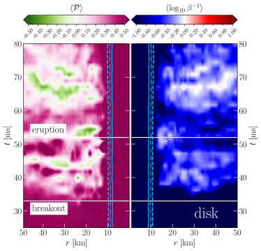
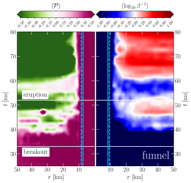
Figure 3: Left panel: Spacetime diagram of the averaged inverse plasma-$\beta$ (right part) and of the averaged Parker-stability criterion (left part); both parts report data associated with the “disk”. Right panel: The same as in the left panel but for the region associated with the “funnel”. Both panels show the time of “breakout” marked with a horizontal white line and blue contours for different rest-mass densities (dashed, dot-dashed and solid lines for $10^{14},\,10^{13.5}$ and $10^{13}\,{\rm g/cm^{3}}$; the latter can be taken as to mark the surface of the HMNS).

3.2 $\alpha$-$\Omega$ dynamo, Parker criterion, and breakout

If the phenomenology discussed so far has a simple and consequential interpretation where, at one point in the evolution, a magnetic breakout takes place yielding a magnetically driven flow that fills the polar region and enhances the EM emission, the actual origin of the instability leading to the breakout still requires a proper explanation. We have mentioned above that after the turbulent amplification of the magnetic field via the KHI, the shearing flows in the HMNS transfer the kinetic and binding energy from the fluid over to the magnetic fields via two main mechanisms. The first one is the simple magnetic winding via the differential rotation in the HMNS leading to the growth of a predominantly toroidal magnetic field. The second one, instead, involves the MRI and produces mostly poloidal magnetic field (see left panel of Fig. 1). Recent simulations of BNS mergers at ultra-high resolution (Kiuchi et al., 2024) have shown the presence of an MRI-driven $\alpha$-$\Omega$ dynamo (Bonanno et al., 2003) in the remnant HMNS, which can lead to the growth of the magnetic field close to the HMNS polar cap and ultimately to a breakout of the field, although the location of the breakout (disk, star or both) will depend crucially on the dynamo processes (Most & Quataert, 2023; Most, 2023).

Our resolution of $\sim 200~{}{\rm m}$ is high but does not allow us to resolve the wavelength of the fastest-growing MRI mode within the high-density region of the HMNS (Siegel et al., 2013), and indeed we do not observe any growth of the magnetic field in regions of rest-mass density $\rho\gtrsim 10^{12}~{}{\rm g/cm^{3}}$ besides linear winding. However, less severe resolutions requirements are needed to resolve the MRI in the inner region of the accretion disc, where the density is $\gtrsim 10^{9}\,{\rm g/cm^{3}}$, which in fact we do resolve accurately. This allows us to point out that a mechanism similar to that reported by Most & Quataert (2023); Combi & Siegel (2023); Kiuchi et al. (2024) can act self-consistently also in the disk and ultimately lead to a buoyant instability with consequent breakout of the magnetic field.

To demonstrate this mechanism, and disentangle the various parts of the flow involved in this complex process, we distinguish the contributions coming from two distinct regions: (i) the “funnel”, i.e., a region near the equatorial plane with radial extent $1<r/{\rm km}<50$ and polar excursion $0<\theta<\pi/6$; (ii) the “disk”, i.e., a region with the same radial extent but around the polar cap, i.e., with $1<r/{\rm km}<50$ and $\pi/6<\theta<\pi/2$. We then use Fig. 3 to report the spacetime diagrams for two quantities relevant to the breakout dynamics: the inverse plasma-$\beta$, and the “Parker-stability criterion” $\mathcal{P}$, namely, a measure of the onset of the magneto-convective instability (Parker, 1966)

$$\mathcal{P}:=\frac{d\log{p}}{d\log{\rho}}-1-\frac{\beta^{-1}\left(1+2\beta^{-1}\right)}{2+3\beta^{-1}}\,.$$ (2)

Both quantities are displayed on the $(x,z)$ plane as an average over the azimuthal angle and refer to either the disk (left panel) or to the funnel (right panel). Within each panel, we distinguish the evolution of the Parker criterion (left side) from that of the inverse plasma-$\beta$ (right side). Furthermore, we mark with light blue lines the worldlines of fluid elements at reference rest-mass densities, i.e., $\log_{10}(\rho)=(13,14,15)\,{\rm g/cm^{3}}$ (solid, dashed, and dot-dashed lines); in this way, the thick solid line can be taken to mark approximately the surface of the remnant HMNS (see Cassing & Rezzolla, 2024, for a detailed discussion).

The four spacetime diagrams in Fig. 3 clearly help realizing that the breakout time marks the moment when the Parker criterion changes sign and hence a buoyant instability is allowed to take place in the disk. The two panels in Fig. 3 also highlight that the conditions in the breakout first take place in the disk and only a few milliseconds later in the funnel. Also apparent is the fact that while the outer regions of the disk are no longer matter-dominated after breakout (dark blue turns to white), it is really the funnel that experiences the largest excursion from a matter-dominated to a magnetically-dominated regime (dark blue turns to dark red); a similar phenomenology has been reported also in other simulations under different approximations but comparable conditions (Kiuchi et al., 2024; Most & Quataert, 2023; Most, 2023).

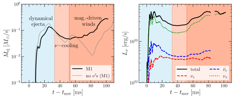
Figure 4: Left panel: Evolution of the ejection rest-mass rate ${\dot{M}}_{\rm ej}$, showing first the peak of the dynamical ejecta and subsequently that the cooling by neutrinos reduces the efficiency of ${\dot{M}}_{\rm ej}$ (the color-shading is the same as in Fig. 1). After eruption, however, the mass-ejection rate increases thanks to the launching of the magnetically-driven winds; a gray line shows the corresponding evolution when no neutrinos are taken into account (no ${\rm M1}$). Right panel: Evolution of the total neutrino luminosity (black solid line) together with the contributions from heavy neutrinos (green dashed line), electron neutrinos and antineutrinos (red and blue dashed lines, respectively).

3.3 Mass ejection and the role of neutrinos

The magnetic-field breakout and eruption also has an impact on the amount of mass that is ejected from the merger remnant. This is illustrated in the left panel of Fig. 4, where we report the rest-mass ejection rate computed as the surface integral of the unbound mass flux (according to the standard “Bernoulli” criterion $hu_{t}<-1$) at the same detector where we measure the Poynting flux. The evolution prior to the eruption shows the well-understood initial burst of unbound material that is commonly referred to as the “dynamical ejection”, i.e., the launching of high specific-entropy material accelerated by the collision of the two merging stars and typically occurring in multiple waves as the stellar cores bounce repeatedly (Bovard et al., 2017; Bernuzzi et al., 2020; Dietrich & Ujevic, 2017; Neuweiler et al., 2023; Papenfort et al., 2018; Most et al., 2021; Zappa et al., 2023). This initial phase of dynamical ejection is followed by a sustained wind of unbound matter (see Fig. 4), which is largely caused by neutrino energy deposition in the funnel (see also the discussion in Appendix B). This “neutrino-driven” wind (Dessart et al., 2009), which kicks-in shortly after merger, dominates at intermediate times between the end of the dynamical ejection phase and the onset of the magnetic ejection and, as we will discuss next, plays an important role in clearing the funnel and promoting the proper conditions for the launching of the outflow.

As can be observed from Fig. 1, after breakout the mass-ejection rate slowly grows together with the Poynting flux, indicating that the unbound material becomes progressively more magnetized. Once the magnetic field completely fills the polar region above the HMNS and the funnel becomes magnetically dominated, the Poynting flux luminosity increases steeply and the wind becomes essentially magnetically driven, forming a jet-like configuration (Lynden-Bell, 1996; Rezzolla et al., 2011; Shibata et al., 2011), which can clearly be observed in Fig. 2. This phenomenology is similar to what is described by Most (2023) in the case of maximum amplification of the turbulent magnetization, where a steady, high-Poynting flux outflow is observed. However, we can highlight for the the first time that a Blandford-Payne magneto-centrifugal mechanism (Blandford & Payne, 1982) is also active and contributing to the the acceleration and collimation of the outflow and quantifiable in terms of the magnetic lever-arm contribution to the fluid energy [see the detailed discussion of Eq. (B1) and Figs. 7-8 in Appendix B].

Overall, the values measured in our simulations are $\dot{M}_{\rm ej}\sim 4-5\times 10^{-2}\,M_{\odot}/{\rm s}$ and hence about a factor two-three larger than those estimated by Gill et al. (2019). The magnetically-driven wind has generally larger speeds than those of the neutrino-driven wind, with the former having Lorentz factors $W\lesssim 1.05$ and terminal Lorentz factors $W_{\infty}:=-h\,u_{t}\lesssim 1.2$, while the latter reaches Lorentz factors of $W\sim 1.1$ and terminal Lorentz factors of $W_{\infty}\sim 1.5$.

The merger obviously lead also to a dramatic change in the thermodynamical state of the neutron stars, raising their temperature from a few eV minutes prior to merger to tens of MeV in the course of a few milliseconds after the merger. As the HMNS reaches a quasi-stationary MHD equilibrium, so does its temperature stratification, which is represented by a dense and relatively cold core surrounded by a hotter ring of rapidly rotating matter, whose temperature gradually decreases when moving outwards to smaller rest-mass densities (see, e.g.,  Kastaun & Galeazzi, 2015; Hanauske et al., 2017). As a result of this quasi-stationary thermodynamical equilibrium, a copious amount of neutrinos are produced and emitted.

In turn, neutrinos are also responsible for the ejection of substantial amounts of matter via neutrino-driven winds, which have been the subject of numerous studies in the context of BNS mergers (Dessart et al., 2009; Perego et al., 2014; Martin et al., 2015; Fujibayashi et al., 2017, 2017). At the risk of oversimplification, these neutrino-driven winds consist in polar outflows with relatively high electron fraction ($0.3\leq Y_{e}\leq 0.5$) and mildly relativistic speeds ($W\lesssim 1.1$). They are caused by transfer of momentum from the neutrinos to the matter in the outer layers of the star and of the high-density regions of the disk. As a result, they contribute to the large mass-ejection rates measured in our simulations prior to breakout. Indeed, until breakout, neutrinos can be considered as the main “driver” of the mass outflow. This can be readily deduced from the rightmost panel in the top row of Fig. 2, which shows the velocity field as a stream-plot. Note the presence of an ordered outflow in the funnel where matter is unbound (see discussion in Appendix B), where however the magnetic field is still very low (see leftmost panel of Fig. 2) and the thermal pressure dominates over the magnetic pressure ($\beta^{-1}\ll 1$). Under these conditions, the source of acceleration of the unbound material in the funnel is not magnetic in origin and hence the outflow is neutrino driven.

The evolution of the neutrino luminosities is shown in the right panel of Fig. 4, where we report the total luminosity (black solid line) and also the contributions coming from heavy neutrinos (green dashed line), electron neutrinos and antineutrinos (red and blue dashed lines, respectively). Note how the main component of the total neutrino luminosity, that reaches values $L_{\nu}\sim 4\times 10^{53}\,{\rm erg/s}$, comes from the heavy neutrinos, whose luminosity is more than twice that of electron neutrinos and antineutrinos. Of course, these considerable losses in energy come at the expense of the thermal and kinetic energies of the system. The former manifests itself in a cooling of the remnant and a corresponding gradual reduction of the neutrino luminosity at about $10\,{\rm ms}$ after merger. Moreover, the energy carried away by neutrinos leads to a reduced dynamical ejection of matter. Indeed, including neutrino transport in simulations of BNS mergers generally reduces the total amount of dynamically ejected material by up to a factor of two compared to simulations that exclude neutrino effects, as can be evinced by comparing the gray and black curves in the left panel of Fig. 4 (see also Zappa et al., 2023). In addition, the absence of neutrino essentially quenches the mass-ejection rate after the dynamical-ejection episode at $\sim 15\,{\rm ms}$ after the merger, and will be necessary to wait for the subsequent breakout, occurring much later and at about $100\,{\rm ms}$ after the merger, to see a significant increase the mass-ejection rate.

Before breakout, neutrinos also play the very important role of “cleaning up” the funnel, namely, of reducing the baryon loading in the funnel and hence promote the breakout of magnetic field from the torus surface. This is clearly correlated with the evolution in the neutrino luminosity, that stops decreasing between breakout and eruption and then increases after eruption (see the black solid line in the right panel of Fig. 4). This is simply the consequence of the fact that the funnel has now been cleaned up of baryons (hence reducing neutrino capture and scattering) and neutrinos can be emitted more easily.

When neutrinos are ignored and the cleaning up does not take place, the polar regions of the remnant are filled with baryon-rich material that cannot be blown out via a neutrino-driven wind. As a result, the mass stops being ejected after the initial dynamical ejection and, as it can be appreciated from the gray line in the left panel of Fig. 4, the mass-ejection rate steadily decreases till $t-t_{\rm mer}\simeq 85\,{\rm ms}$, when it is revived by the magnetic breakout. More importantly, the baryon pollution outside the HMNS prevents the expulsion of magnetic field from the disk surface, which takes place at $t-t_{\rm mer}\simeq 35\,{\rm ms}$, when neutrinos are accounted for. Much larger magnetic fields will have to be produced via winding to reach the critical Parker-stability limit and start launching and magnetically driven outflow. This is particularly clear when looking at the right panel of Fig. 1, where the solid gray line shows how the EM luminosity is essentially constant at the eruption of magnetic field takes place at $t-t_{\rm mer}\simeq 80\,{\rm ms}$ (the breakout in this case happens somewhat earlier, i.e., at $t-t_{\rm mer}\sim 50\,{\rm ms}$; see also Fig. 6 in Appendix B). This result, should help resolve the on-going debate within the literature and concerned on whether neutrinos or magnetic fields are responsible for the generation a powerful and collimated but non-relativistic outflow (Ciolfi, 2020; Mösta et al., 2020). The black and gray lines in the right panel in Fig. 1 address this question beyond debate and clearly show what we have already anticipated: neutrinos play an important and promoting role in launching a magnetically-driven outflow but are not strictly necessary. To the best of our knowledge this is the first time that point is addressed with self-consistent GRMHD and M1 neutrino-transfer calculations (see also Combi & Siegel, 2023, for one-moment approaches).

4 Conclusion

Whether the metastable remnant of a BNS merger can launch a relativistic, magnetized and collimated outflow has been a matter of debate over the last few years, with different approaches reaching different conclusions. Examples include the development of magnetically-driven outflows for simplified microphysics treatments (e.g.,  Ciolfi, 2020; Pavan et al., 2023; Bamber et al., 2024), or simplified magnetic-field evolutions with more realistic neutrino microphysics (e.g.,  Mösta et al., 2020; de Haas et al., 2023; Curtis et al., 2024)), or both (Combi & Siegel, 2023). Recently, several works have also investigated the importance of dynamo processes (Most & Quataert, 2023; Most, 2023; Kiuchi, 2024) as a prerequisite for field breakout and the formation of a collimated outflow. With the goal of clarifying this picture in particular with regards to the importance and role of neutrinos, we have carried out long-term simulations of the inspiral, merger and post-merger evolution of a BNS system in which both magnetic fields and neutrino absorption and emission are properly described. In addition, we have replicated the same simulation setup neglecting neutrinos, so as to highlight and distinguish the role played by magnetic fields and neutrinos.

This analysis has allowed us to reach a number of conclusions, which we briefly summarise below. First, right after merger an intense neutrino emission takes place that generates a neutrino-driven wind and “clears-up” the polar region above the remnant from matter. Second, after $\sim~{}50\,{\rm ms}$ from the merger, a dynamo driven by the MRI develops in the densest regions of the disk and leads to the breakout of the magnetic field lines in the polar region. Third, the breakout, which can be directly associated with the violation of the Parker-instability criterion and is responsible for a collimated, magnetically driven, Poynting-flux dominated outflow with only mildly relativistic velocities. Based on higher Lorentz factors reached in very high resolution studies (Kiuchi, 2024), we speculate that the details may strongly depend on the regions where the dynamo is active and breakout eventually happens. The outflow we observe is partly accelerated and collimated via a Blandford-Payne mechanism driven by the open field lines anchored in the inner-disk regions. Finally, contrasting the simulations with and without neutrino transport we were able to ascertain that the physical mechanism of magnetic-field breakout is robust and takes place even without neutrinos. The latter, however, lead to a cooler, geometrically thinner disk and a lower degree of baryon pollution in polar regions, hence anticipating the occurrence of the breakout and yielding a larger Poynting flux.

The overall conclusion of this work is that while magnetically-driven and magnetically-confined outflows can and are produced robustly from the metastable merger remnant of BNS mergers, the associated jet-like outflows launched via disk-driven breakout are only mildly relativistic nature. In the absence of additional field amplification in denser regions (Kiuchi, 2024) (however, see also Aguilera-Miret et al. (2024)), the mechanism presented here might be insufficient to account for outflows responsible for powering short gamma-ray bursts. However, a more conclusive statement will have to wait for new simulations of this type at even larger resolutions, or using suitably tuned effective mean-field dynamo models (Most, 2023). These are needed in order to properly resolve the MRI also in the regions of the HMNS with the highest magnetic fields and densities, which are precluded from our analysis with the present resolution. While these regions are much smaller in size than the those involved in the magnetic breakout from the disk (i.e., $\sim 10\,{\rm km}$ vs $\sim 50\,{\rm km}$) and will not prevent the breakout observed here, it is possible that they will also contribute to the breakout and hence to the launching of collimated and magnetically-driven winds from the remnant. We will assess this possibility in future studies.

Appendix A Simulations without neutrino transfer

As already mentioned in several instances in the main text, the study carried out here and the results obtained are corroborated by a parallel set of simulations in which neutrino radiative transfer via an M1 approach is neglected. Of course, we do not neglect neutrinos because unimportant. Rather, since this is still a matter of a lively debate, we do so in order to disentangle their role from that of magnetic fields and assess whether they are necessary to launch a magnetically-driven and collimated outflow or not.

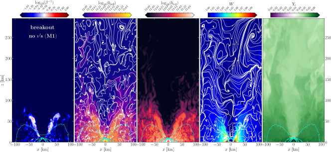
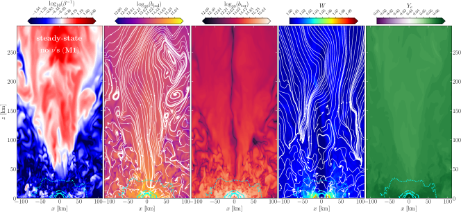
Figure 5: The same as in Fig. 2 but for a GRMHD simulation without neutrino transfer. Note that the breakout still takes place but at much later times ($t-t_{\rm mer}\simeq 50\,{\rm ms}$) and that the steady-state ($t-t_{\rm mer}\simeq 100\,{\rm ms}$) shows weaker, less collimated and slower outflows. Note the considerably different rage in which $Y_{e}$ is shown.

Figure 1 reports with gray lines of various type the evolution of the corresponding quantities when neutrinos are neglected (no ${\rm M1}$) and clearly shows that neglecting neutrinos does not introduce a qualitative change in the evolution of the magnetic energy (left panel) or of the EM luminosity (right panel). At the same time, and from a more quantitative point of view, it also highlights that neutrinos do actually facilitate the breakout, anticipating it by several tens of milliseconds.

Another qualitative and quantitative comparison between the two scenarios is offered in Fig. 5, which is the same as in Fig. 2, but for a GRMHD simulation without neutrino transfer, and where it should be noted the considerably different range in which $Y_{e}$ is shown. Note that the breakout still takes place but at much later times ($t-t_{\rm mer}\simeq 50\,{\rm ms}$) and that before breakout both the poloidal and toroidal magnetic fields are stronger than when considering neutrinos. This is because the remnant is not losing kinetic and binding energy via neutrinos and hence it is more efficient in converting the latter two into magnetic energy, thus amplifying the magnetic-field strength after merger (see also the left panel of Fig. 1). In addition, the lack of neutrinos and the corresponding neutrino-driven winds implies that when a steady-state is reached ($t-t_{\rm mer}\simeq 100\,{\rm ms}$), a larger baryon pollution is present in the remnant’s polar regions and that the corresponding poloidal magnetic-field component will be more irregular and with a smaller large-scale component. As a result, the magnetically-driven outflow will be shows weaker, less collimated and slower.

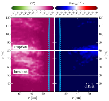
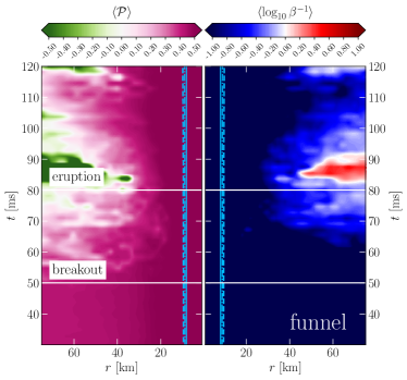
Figure 6: The same as in Fig. 3 but for a GRMHD simulation without neutrino transfer.

Figure 6 provides another point of comparison by offering the equivalent of the spacetime diagrams presented in Fig. 6 in the case when neutrino are neglected. Note that the qualitative behaviour is the same and that a sharp transition takes place when the Parker-stability criterion is violated. Also in this case, the inverse plasma-$\beta$ goes from being very small to being very large. However, the time when this takes place is considerably later and the breakout can here be seen to start at $t-t_{\rm mer}\simeq 50\,{\rm ms}$.

In summary, the discussion presented here, combined with that in the main text, reinforces a point we have already highlighted repeatedly: while neutrinos promoting and speed-up the magnetic breakout, they are not necessary. When neglected, a magnetically-driven wind will be produced nevertheless, although it will be less collimated and with smaller Lorentz factors. In either case, it is difficult to associate these outflows with the ultra-relativistic jets expects in short gamma-ray bursts.

Appendix B Decomposition of outflow energetics

Having in mind the description of the mass-ejection dynamics discussed in the main text, we now switch to a more quantitative discussion of the energetics of the magnetically-driven winds with the scope of determining the role and weight played by the various contributions in generating the outflow. To this end, we consider a “magnetized extension” of the classic Bernoulli criterion (Rezzolla & Zanotti, 2013) that is customarily used to determine whether an unmagnetized fluid element is gravitationally bound to a gravitational field central object. More specifically, assuming a stationary and axisymmetric spacetime, we consider a magnetized fluid element unbound if (Bekenstein & Oron, 1978; Gourgoulhon et al., 2011).

$$\left(h+\frac{b^{2}}{\rho}\right)u_{t}-\frac{b_{t}}{\kappa}<-1\,,$$ (B1)

where, again, $h$ is specific enthalpy of the fluid, $b$ and $b_{t}$ are respectively the strength of the magnetic field in the comoving frame and its covariant time component, $-u_{t}$ is the fluid energy at infinity (i.e., the covariant time component of the fluid four-velocity), and $\kappa:=\rho u^{\rm pol}/b^{\rm pol}$ is proportional to the ratio of the kinetic-to-magnetic energies in the comoving frame (in a spherical coordinate system, $u^{\rm pol}:=\sqrt{[(u^{\theta})^{2}+(u^{r})^{2}]/2}$).

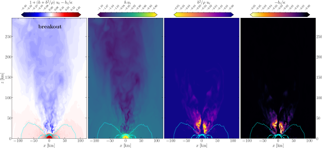
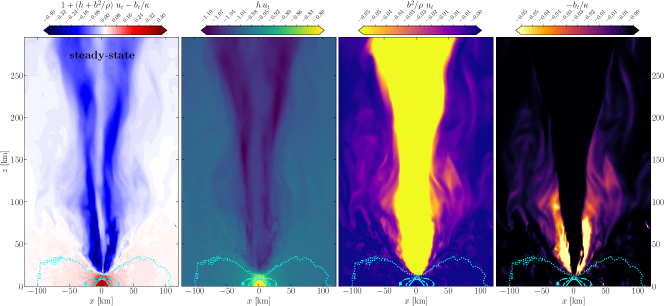
Figure 7: Two-dimensional distributions in the $(x,z)$ plane of various terms contributing to the extended Bernoulli criterion in Eq. (B1). Shown from left to right are: the extended Bernoulli criterion $1+(h+b^{2}/\rho)~{}u_{t}-b_{t}/\kappa$, the geodesic criterion $h\,u_{t}$, the magnetization $b^{2}/\rho$, and the magneto-centrifugal contribution $b_{t}/\kappa$. The top row refers to the breakout time, while the bottom row to the steady-state stage; neutrinos are properly accounted in these simulations; see also Fig. 2.

We can now analyse separately the various terms in Eq. (B1). Starting from the left, the first term $h\,u_{t}$ is the classic and the purely kinetic “geodesic” term that is traditionally considered when judging whether or not a fluid element is bound or not (see, e.g.,  Bovard & Rezzolla, 2017; Musolino et al., 2024, for a detailed discussion). The second term, on the other hand, is magnetic in origin and is often referred to as the “magnetisation” of the plasma, $\sigma:=b^{2}/\rho$, that is, the ratio of magnetic-to-rest-mass energy of the fluid. This term accounts therefore for the purely magnetic energy reservoir that can accelerate the plasma generating an outflow; the larger $\sigma$, the larger the weight of the magnetic field and, of course, $\sigma>1$ signals a magnetically-dominated plasma. Finally, the third term in (B1), expresses the ratio between the toroidal magnetic field and th so-called “mass-loading” parameter $\kappa$ that is a combination of the poloidal components of the fluid velocity and of the poloidal comoving magnetic field. As a result, in the Newtonian limit the whole term $b_{t}/\kappa$ reduces to a magnetic lever-arm contribution to the total fluid energy (Zhu & Stone, 2018). This last term, while only active in the outer layers of the wind, provides an important contribution to the conserved energy of fluid elements in that region, and is responsible for a Blandford-Payne type magneto-centrifugal acceleration and collimation of the wind. Indeed, Blandford-Payne winds in the context of Newtonian astrophysical simulations are identified precisely through the evaluation of this energy component, which is observed here for the first time in a general-relativistic context. Clearly, the larger the third term in Eq. (B1), the larger the Blandford-Payne magneto-centrifugal acceleration imparted on the fluid.

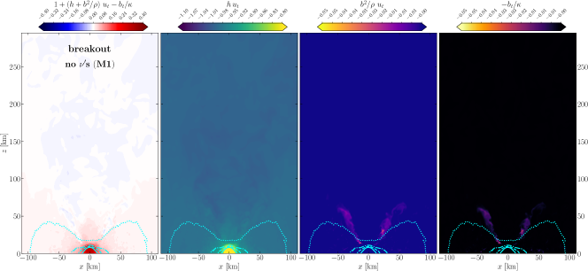
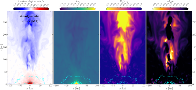
Figure 8: The same as in Fig. 7 but when neutrinos are not taken into account; see also Fig. 2.

Figure 7 provides two snapshots of all of these terms at either the breakout time (top row) or in the steady-state phase (bottom row). More specifically, from left to right, we present the extended Bernoulli criterion $1+(h+b^{2}/\rho)~{}u_{t}-b_{t}/\kappa$, the geodesic criterion $h\,u_{t}$, the magnetization $b^{2}/\rho$, and the magneto-centrifugal contribution $b_{t}/\kappa$. When looking at the top row, it is then apparent that at breakout only a mild wind is present (first two panels from left) and that this wind is neutrino-driven, given that the magnetization in the funnel is very small (third panel from left; compare also with the first two panels in Fig. 8) and is larger at the edges of the disk, exactly where the $\alpha$-$\Omega$ dynamo will lead to the breakout of the magnetic field. At this stage, the magneto-centrifugal acceleration (rightmost panel) is clearly very small. On the other hand, exploring the bottom row in the steady-state stage, it is clear that a strong unbound wind is launched (first two panels from left) and that this is magnetically-driven, given the very large magnetization in the funnel (third panel from left). Importantly, note how at this point the magneto-centrifugal acceleration provides a significant contribution and that this is essentially absent in the regions very close to the pole. This is simply because there is no lever-arm to produce a magneto-centrifugal acceleration there, and this can be active only in the upper edges of the disk. To the best of our knowledge, this is the first time that a Blandford-Payne type of acceleration is shown to be active in the metastable remnant from a BNS merger.

Figure 8 provides the same type of diagnostic shown in Fig. 7 but for the GRMHD simulations that have neglected neutrino transport (no ${\rm M1}$). Contrasting the top rows of the two figures, it is very simple (and obvious) to recognise that no neutrino-driven wind is present in this latter case, but also that no magneto-centrifugal acceleration can be observed. This provides a very robust evidence that the outflowing wind measured before breakout is generated by neutrinos. Similarly, when contrasting the bottom rows of the two figures it is east to capture the very similar qualitative behaviour of the outflows. However, as already commented for other fluid quantities, the lack of neutrinos in Fig. 8 implies that the baryon pollution affects the outflow, which is therefore less collimated, less magnetized and with a smaller Blandford-Payne contribution. The disk too is impacted by the absence of neutrinos and of the associated cooling. As a result, the disk will be more extended in on the equatorial plane and also with a larger thickness (compare the top rows of Figs.7 and 8), making the breakout harder to achieve. While our simulations end at about $t-t_{\rm mer}\sim 110\,{\rm ms}$, it is reasonable to assume that that the bottom panels of Figure 8 will resemble closely those of Fig. 7 on sufficiently large timescales.

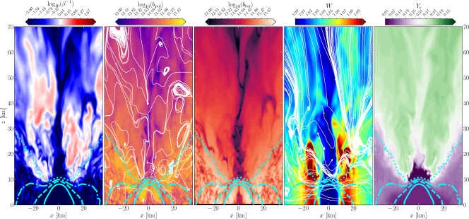
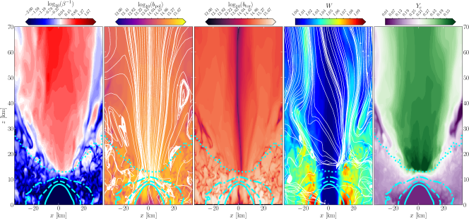
Figure 9: The same as Fig. 2 but on a smaller scale to highlight features near the HMNS.

Appendix C Close-up view of the plasma properties

We have already commented on the features of Fig. 2 and how the two rows illustrate the status of various properties of the plasma at breakout (top bottom rows and in the steady-state stage (bottom row). Figure 9 provides the same information but when zooming-in on lengthscales that are representative of the HMNS. In this case, a number of features can be appreciated at breakout: (i) the breakout clearly takes place from the disk and not from the HMNS and, in particular, from plasma at densities between $10^{11}$ and $10^{12}\,{\rm G}$; (ii) the toroidal magnetic field is weak along the rotation axis and essentially zero in the core of the HMNS; (iii) because of the high differential rotation of the HMNS, the maximum velocity and hence Lorentz factors are achieved at $\simeq 10$-$15\,{\rm km}$ from the rotation axis and are very small on the rotation axis because of the axial symmetry; (iv) the regions where neutrinos start to modify the electron fraction coincide with those where the breakout takes place, leaving the regions very close to the pole of the HMNS with very small values of $Y_{e}$. On the other hand, in the late steady-state stage we note that: (i) the magnetically-driven wind now comes also from the polar regions of the HMNS, filling the funnel completely; (ii) the regions where the toroidal magnetic field is weak reduce considerably and are only along the rotation axis; (iii) because of high-speed magnetically driven wind, the regions where breakout took place, i.e., on the disk edges, have much lower velocities now in the azimuthal direction, while differential rotation in the HMNS does not change considerably; (iv) the regions very close to the pole of the HMNS have now larger values of $Y_{e}$ and although this is true for the whole funnel, rapid changes still take place when moving from the center to the pole of the HMNS.

Data Availability

Data is available upon reasonable request from the corresponding author.

References

- Abbott et al. (2017) Abbott, B. P., Abbott, R., Abbott, T. D., et al. 2017, Phys. Rev. Lett., 119, 161101, doi: 10.1103/PhysRevLett.119.161101
- Aguilera-Miret et al. (2024) Aguilera-Miret, R., Palenzuela, C., Carrasco, F., Rosswog, S., & Viganò, D. 2024. https://arxiv.org/abs/2407.20335
- Aguilera-Miret et al. (2020) Aguilera-Miret, R., Viganò, D., Carrasco, F., Miñano, B., & Palenzuela, C. 2020, Phys. Rev. D, 102, 103006, doi: 10.1103/PhysRevD.102.103006
- Aguilera-Miret et al. (2022) Aguilera-Miret, R., Viganò, D., & Palenzuela, C. 2022, Astrophys. J. Lett., 926, L31, doi: 10.3847/2041-8213/ac50a7
- Baiotti & Rezzolla (2017) Baiotti, L., & Rezzolla, L. 2017, Rept. Prog. Phys., 80, 096901, doi: 10.1088/1361-6633/aa67bb
- Bamber et al. (2024) Bamber, J., Tsokaros, A., Ruiz, M., & Shapiro, S. L. 2024, Phys. Rev. D, 110, 024046, doi: 10.1103/PhysRevD.110.024046
- Banik et al. (2014) Banik, S., Hempel, M., & Bandyopadhyay, D. 2014, Astrohys. J. Suppl., 214, 22, doi: 10.1088/0067-0049/214/2/22
- Bekenstein & Oron (1978) Bekenstein, J. D., & Oron, E. 1978, Phys. Rev. D, 18, 1809, doi: 10.1103/PhysRevD.18.1809
- Bernuzzi et al. (2020) Bernuzzi, S., Breschi, M., Daszuta, B., et al. 2020, arXiv e-prints, arXiv:2003.06015. https://arxiv.org/abs/2003.06015
- Blandford & Payne (1982) Blandford, R. D., & Payne, D. G. 1982, Mon. Not. R. Astron. Soc., 199, 883
- Bonanno et al. (2003) Bonanno, A., Rezzolla, L., & Urpin, V. 2003, Astron. Astrophys., 410, L33. https://arxiv.org/abs/astro-ph/0309783
- Bovard et al. (2017) Bovard, L., Martin, D., Guercilena, F., et al. 2017, Phys. Rev. D, 96, 124005. https://arxiv.org/abs/1709.09630
- Bovard & Rezzolla (2017) Bovard, L., & Rezzolla, L. 2017, Classical and Quantum Gravity, 34, 215005, doi: 10.1088/1361-6382/aa8d98
- Cassing & Rezzolla (2024) Cassing, M., & Rezzolla, L. 2024, Mon. Not. R. Astron. Soc., 532, 945, doi: 10.1093/mnras/stae1527
- Chabanov & Rezzolla (2023) Chabanov, M., & Rezzolla, L. 2023, arXiv e-prints, arXiv:2307.10464, doi: 10.48550/arXiv.2307.10464
- Chabanov et al. (2023) Chabanov, M., Tootle, S. D., Most, E. R., & Rezzolla, L. 2023, Astrophys. J. Lett., 945, L14, doi: 10.3847/2041-8213/acbbc5
- Christie et al. (2019) Christie, I. M., Lalakos, A., Tchekhovskoy, A., et al. 2019, Mon. Not. R. Astron. Soc., 490, 4811, doi: 10.1093/mnras/stz2552
- Ciolfi (2020) Ciolfi, R. 2020, Mon. Not. R. Astron. Soc., 495, L66, doi: 10.1093/mnrasl/slaa062
- Combi & Siegel (2023) Combi, L., & Siegel, D. M. 2023, Phys. Rev. Lett., 131, 231402, doi: 10.1103/PhysRevLett.131.231402
- Curtis et al. (2024) Curtis, S., Bosch, P., Mösta, P., et al. 2024, ApJ, 961, L26, doi: 10.3847/2041-8213/ad0fe1
- de Haas et al. (2023) de Haas, S., Bosch, P., Mösta, P., Curtis, S., & Schut, N. 2023, Mon. Not. Roy. Astron. Soc., 527, 2240, doi: 10.1093/mnras/stad2931
- Dessart et al. (2009) Dessart, L., Ott, C. D., Burrows, A., Rosswog, S., & Livne, E. 2009, Astrophys. J., 690, 1681, doi: 10.1088/0004-637X/690/2/1681
- Dietrich & Ujevic (2017) Dietrich, T., & Ujevic, M. 2017, Classical and Quantum Gravity, 34, 105014, doi: 10.1088/1361-6382/aa6bb0
- East et al. (2019) East, W. E., Paschalidis, V., Pretorius, F., & Tsokaros, A. 2019, Phys. Rev. D, 100, 124042, doi: 10.1103/PhysRevD.100.124042
- Etienne et al. (2010) Etienne, Z. B., Liu, Y. T., & Shapiro, S. L. 2010, Phys. Rev. D, 82, 084031, doi: 10.1103/PhysRevD.82.084031
- Etienne et al. (2015) Etienne, Z. B., Paschalidis, V., Haas, R., Mösta, P., & Shapiro, S. L. 2015, Class. Quantum Grav., 32, 175009, doi: 10.1088/0264-9381/32/17/175009
- Etienne et al. (2012) Etienne, Z. B., Paschalidis, V., Liu, Y. T., & Shapiro, S. L. 2012, Phys. Rev. D, 85, 024013, doi: 10.1103/PhysRevD.85.024013
- Fujibayashi et al. (2017) Fujibayashi, S., Sekiguchi, Y., Kiuchi, K., & Shibata, M. 2017, The Astrophysical Journal, 846, 114, doi: 10.3847/1538-4357/aa8039
- Fujibayashi et al. (2017) Fujibayashi, S., Sekiguchi, Y., Kiuchi, K., & Shibata, M. 2017, ApJ, 846, 114, doi: 10.3847/1538-4357/aa8039
- Giacomazzo et al. (2009) Giacomazzo, B., Rezzolla, L., & Baiotti, L. 2009, Mon. Not. R. Astron. Soc., 399, L164, doi: 10.1111/j.1745-3933.2009.00745.x
- Giacomazzo et al. (2011) Giacomazzo, B., Rezzolla, L., & Baiotti, L. 2011, Phys. Rev. D, 83, 044014, doi: 10.1103/PhysRevD.83.044014
- Gill et al. (2019) Gill, R., Nathanail, A., & Rezzolla, L. 2019, Astrophys. J., 876, 139, doi: 10.3847/1538-4357/ab16da
- Gottlieb et al. (2023a) Gottlieb, O., et al. 2023a, Astrophys. J. Lett., 954, L21, doi: 10.3847/2041-8213/aceeff
- Gottlieb et al. (2023b) Gottlieb, O., Metzger, B. D., Quataert, E., et al. 2023b, Astrophys. J. Lett., 958, L33, doi: 10.3847/2041-8213/ad096e
- Gourgoulhon et al. (2011) Gourgoulhon, E., Markakis, C., Uryū, K., & Eriguchi, Y. 2011, Physical Review D, 83, doi: 10.1103/physrevd.83.104007
- Haas & et al. (2020) Haas, R., & et al. 2020, The Einstein Toolkit, The ”DeWitt-Morette” release, ET_2020_11, Zenodo, doi: 10.5281/zenodo.4298887
- Hanauske et al. (2017) Hanauske, M., Takami, K., Bovard, L., et al. 2017, Phys. Rev. D, 96, 043004, doi: 10.1103/PhysRevD.96.043004
- Hilditch et al. (2013) Hilditch, D., Bernuzzi, S., Thierfelder, M., et al. 2013, Phys. Rev. D, 88, 084057, doi: 10.1103/PhysRevD.88.084057
- Jacquemin-Ide et al. (2024) Jacquemin-Ide, J., Rincon, F., Tchekhovskoy, A., & Liska, M. 2024, Mon. Not. Roy. Astron. Soc., 532, 1522, doi: 10.1093/mnras/stae1538
- Kastaun & Galeazzi (2015) Kastaun, W., & Galeazzi, F. 2015, Phys. Rev. D, 91, 064027, doi: 10.1103/PhysRevD.91.064027
- Kiuchi (2024) Kiuchi, K. 2024, arXiv preprint arXiv:2405.10081
- Kiuchi et al. (2015a) Kiuchi, K., Cerdá-Durán, P., Kyutoku, K., Sekiguchi, Y., & Shibata, M. 2015a, Phys. Rev. D, 92, 124034, doi: 10.1103/PhysRevD.92.124034
- Kiuchi et al. (2018) Kiuchi, K., Kyutoku, K., Sekiguchi, Y., & Shibata, M. 2018, Phys. Rev. D, 97, 124039, doi: 10.1103/PhysRevD.97.124039
- Kiuchi et al. (2024) Kiuchi, K., Reboul-Salze, A., Shibata, M., & Sekiguchi, Y. 2024, Nature Astronomy, 8, 298, doi: 10.1038/s41550-024-02194-y
- Kiuchi et al. (2015b) Kiuchi, K., Sekiguchi, Y., Kyutoku, K., et al. 2015b, Phys. Rev. D, 92, 064034, doi: 10.1103/PhysRevD.92.064034
- Lehner et al. (2016) Lehner, L., Liebling, S. L., Palenzuela, C., et al. 2016, Classical and Quantum Gravity, 33, 184002, doi: 10.1088/0264-9381/33/18/184002
- Liska et al. (2018) Liska, M. T. P., Tchekhovskoy, A., & Quataert, E. 2018, arXiv e-prints, arXiv:1809.04608. https://arxiv.org/abs/1809.04608
- Liu & Shapiro (2004) Liu, Y. T., & Shapiro, S. L. 2004, Phys. Rev. D, 69, 044009, doi: 10.1103/PhysRevD.69.044009
- Liu et al. (2008) Liu, Y. T., Shapiro, S. L., Etienne, Z. B., & Taniguchi, K. 2008, Phys. Rev. D, 78, 024012, doi: 10.1103/PhysRevD.78.024012
- Londrillo & Del Zanna (2004) Londrillo, P., & Del Zanna, L. 2004, Journal of Computational Physics, 195, 17
- Lynden-Bell (1996) Lynden-Bell, D. 1996, Mon. Not. R. Astron. Soc., 279, 389, doi: 10.1093/mnras/279.2.389
- Martin et al. (2015) Martin, D., Perego, A., Arcones, A., et al. 2015, Astrophys. J., 813, 2, doi: 10.1088/0004-637X/813/1/2
- Metzger & Fernández (2014) Metzger, B. D., & Fernández, R. 2014, Mon. Not. R. Astron. Soc., 441, 3444, doi: 10.1093/mnras/stu802
- Mizuno & Rezzolla (2024) Mizuno, Y., & Rezzolla, L. 2024, arXiv e-prints, arXiv:2404.13824, doi: 10.48550/arXiv.2404.13824
- Most (2023) Most, E. R. 2023, Phys. Rev. D, 108, 123012, doi: 10.1103/PhysRevD.108.123012
- Most et al. (2020) Most, E. R., Jens Papenfort, L., Dexheimer, V., et al. 2020, Eur. Phys. J. A, 56, 59, doi: 10.1140/epja/s10050-020-00073-4
- Most et al. (2019) Most, E. R., Papenfort, L. J., Dexheimer, V., et al. 2019, Phys. Rev. Lett., 122, 061101, doi: 10.1103/PhysRevLett.122.061101
- Most et al. (2019) Most, E. R., Papenfort, L. J., & Rezzolla, L. 2019, Mon. Not. R. Astron. Soc., 490, 3588, doi: 10.1093/mnras/stz2809
- Most et al. (2021) Most, E. R., Papenfort, L. J., Tootle, S. D., & Rezzolla, L. 2021, Astrophys. J., 912, 80, doi: 10.3847/1538-4357/abf0a5
- Most & Quataert (2023) Most, E. R., & Quataert, E. 2023, Astrophys. J. Lett., 947, L15, doi: 10.3847/2041-8213/acca84
- Mösta et al. (2020) Mösta, P., Radice, D., Haas, R., Schnetter, E., & Bernuzzi, S. 2020, Astrophys. J. Lett., 901, L37, doi: 10.3847/2041-8213/abb6ef
- Murguia-Berthier et al. (2021) Murguia-Berthier, A., Ramirez-Ruiz, E., De Colle, F., et al. 2021, Astrophys. J., 908, 152, doi: 10.3847/1538-4357/abd08e
- Murguia-Berthier et al. (2016) Murguia-Berthier, A., Ramirez-Ruiz, E., Montes, G., et al. 2016, Astrophys. J. Lett., 835, L34, doi: 10.3847/2041-8213/aa5b9e
- Musolino et al. (2024) Musolino, C., Duqué, R., & Rezzolla, L. 2024, Astrophys. J. Lett., 966, L31, doi: 10.3847/2041-8213/ad3bb3
- Musolino & Rezzolla (2024) Musolino, C., & Rezzolla, L. 2024, Mon. Not. R. Astron. Soc., 528, 5952, doi: 10.1093/mnras/stae224
- Neuweiler et al. (2023) Neuweiler, A., Dietrich, T., Bulla, M., et al. 2023, Phys. Rev. D, 107, 023016, doi: 10.1103/PhysRevD.107.023016
- Palenzuela et al. (2022) Palenzuela, C., Aguilera-Miret, R., Carrasco, F., et al. 2022, Phys. Rev. D, 106, 023013, doi: 10.1103/PhysRevD.106.023013
- Palenzuela et al. (2015) Palenzuela, C., Liebling, S. L., Neilsen, D., et al. 2015, Phys. Rev. D, 92, 044045, doi: 10.1103/PhysRevD.92.044045
- Papenfort et al. (2018) Papenfort, L. J., Gold, R., & Rezzolla, L. 2018, Phys. Rev. D, 98, 104028, doi: 10.1103/PhysRevD.98.104028
- Papenfort et al. (2022) Papenfort, L. J., Most, E. R., Tootle, S., & Rezzolla, L. 2022, Mon. Not. Roy. Astron. Soc., 513, 3646, doi: 10.1093/mnras/stac964
- Papenfort et al. (2021) Papenfort, L. J., Tootle, S. D., Grandclément, P., Most, E. R., & Rezzolla, L. 2021, Phys. Rev. D, 104, 024057, doi: 10.1103/PhysRevD.104.024057
- Parker (1966) Parker, E. N. 1966, Astrophys. J., 145, 811, doi: 10.1086/148828
- Paschalidis (2017) Paschalidis, V. 2017, Classical and Quantum Gravity, 34, 084002, doi: 10.1088/1361-6382/aa61ce
- Pavan et al. (2023) Pavan, A., Ciolfi, R., Kalinani, J. V., & Mignone, A. 2023, Monthly Notices of the Royal Astronomical Society, 524, 260, doi: 10.1093/mnras/stad1809
- Perego et al. (2014) Perego, A., Rosswog, S., Cabezón, R. M., et al. 2014, Mon. Not. R. Astron. Soc., 443, 3134, doi: 10.1093/mnras/stu1352
- Price & Rosswog (2006) Price, D. J., & Rosswog, S. 2006, Science, 312, 719, doi: 10.1126/science.1125201
- Radice & Bernuzzi (2023) Radice, D., & Bernuzzi, S. 2023, arXiv preprint arXiv:2306.13709
- Radice et al. (2016) Radice, D., Bernuzzi, S., & Ott, C. D. 2016, Phys. Rev. D, 94, 064011, doi: 10.1103/PhysRevD.94.064011
- Rezzolla et al. (2011) Rezzolla, L., Giacomazzo, B., Baiotti, L., et al. 2011, Astrophys. J. Letters, 732, L6, doi: 10.1088/2041-8205/732/1/L6
- Rezzolla & Zanotti (2013) Rezzolla, L., & Zanotti, O. 2013, Relativistic Hydrodynamics (Oxford University Press), doi: 10.1093/acprof:oso/9780198528906.001.0001
- Ruediger & Kichatinov (1993) Ruediger, G., & Kichatinov, L. L. 1993, A&A, 269, 581
- Shibata et al. (2011) Shibata, M., Suwa, Y., Kiuchi, K., & Ioka, K. 2011, Astrophys. J.l, 734, L36, doi: 10.1088/2041-8205/734/2/L36
- Siegel et al. (2013) Siegel, D. M., Ciolfi, R., Harte, A. I., & Rezzolla, L. 2013, Phys. Rev. D R, 87, 121302, doi: 10.1103/PhysRevD.87.121302
- Siegel et al. (2014) Siegel, D. M., Ciolfi, R., & Rezzolla, L. 2014, Astrophys. J., 785, L6, doi: 10.1088/2041-8205/785/1/L6
- Tootle (2024) Tootle, S., e. a. 2024, in preparation. https://arxiv.org/abs/in preparation
- Topolski et al. (2024) Topolski, K., Tootle, S. D., & Rezzolla, L. 2024, Astrophys. J., 960, 86, doi: 10.3847/1538-4357/ad0152
- Uryū et al. (2017) Uryū, K., Tsokaros, A., Baiotti, L., et al. 2017, Phys. Rev. D, 96, 103011, doi: 10.1103/PhysRevD.96.103011
- Zappa et al. (2023) Zappa, F., Bernuzzi, S., Radice, D., & Perego, A. 2023, Mon. Not. R. Astron. Soc., 520, 1481, doi: 10.1093/mnras/stad107
- Zhu & Stone (2018) Zhu, Z., & Stone, J. M. 2018, The Astrophysical Journal, 857, 34, doi: 10.3847/1538-4357/aaafc9