Don’t Cut Corners: Exact Conditions for Modularity in Biologically Inspired Representations

Abstract

Why do biological and artificial neurons sometimes modularise, each encoding a single meaningful variable, and sometimes entangle their representation of many variables? In this work, we develop a theory of when biologically inspired representations—those that are nonnegative and energy efficient—modularise with respect to source variables (sources). We derive necessary and sufficient conditions on a sample of sources that determine whether the neurons in an optimal biologically-inspired linear autoencoder modularise. Our theory applies to any dataset, extending far beyond the case of statistical independence studied in previous work. Rather, we show that sources modularise if their support is “sufficiently spread”. From this theory, we extract and validate predictions in a variety of empirical studies on how data distribution affects modularisation in nonlinear feedforward and recurrent neural networks trained on supervised and unsupervised tasks. Furthermore, we apply these ideas to neuroscience data. First, we explain why two studies that recorded prefrontal activity in working memory tasks conflict on whether memories are encoded in orthogonal subspaces: the support of the sources differed due to a critical discrepancy in experimental protocol. Second, we use similar arguments to understand why preparatory and potent subspaces in RNN models of motor cortex are only sometimes orthogonal. Third, we study spatial and reward information mixing in entorhinal recordings, and show our theory matches data better than previous work. And fourth, we suggest a suite of surprising settings in which neurons can be (or appear) mixed selective, without requiring complex nonlinear readouts as in traditional theories. In sum, our theory prescribes precise conditions on when neural activities modularise, providing tools for inducing and elucidating modular representations in brains and machines.

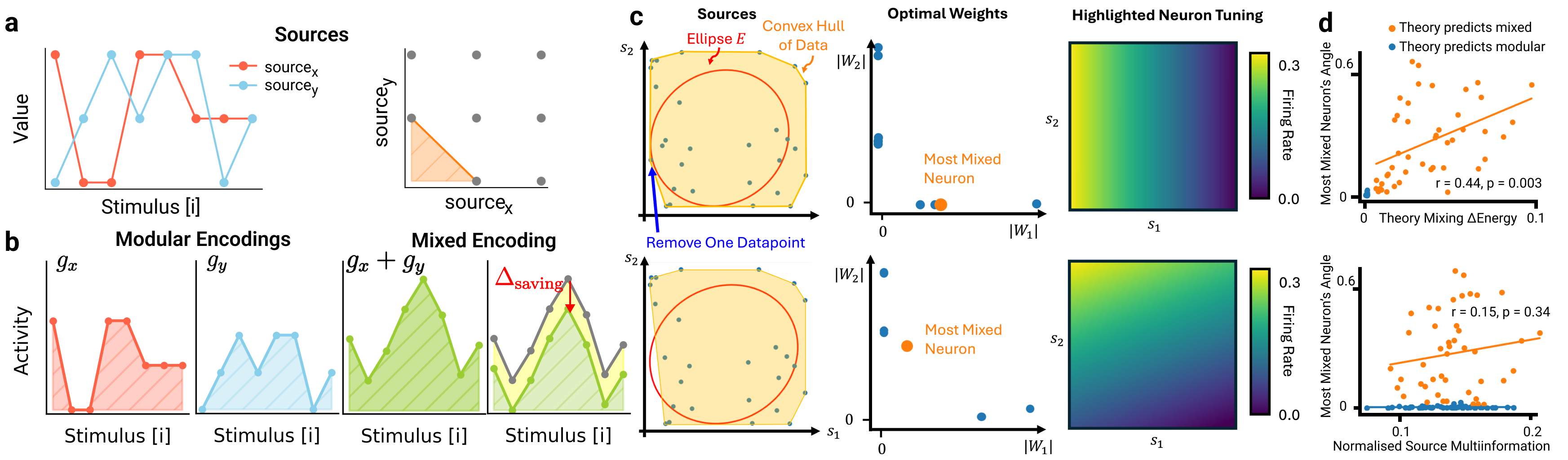
Figure 1: a) Values of two sources as a stimulus varies (left) and corresponding source distribution (right). A corner is missing. b) Whether a biologically inspired model constrained to have a nonnegative and energy efficient latent representation will modularise (left) or mix (right) the sources depends on the relative energy costs. c) Our modularisation conditions (Theorem 2.1) are equivalent to whether the data convex hull encloses a data-dependent ellipse (Theorem 2.2). The precision of these conditions is validated in two experiments (rows) in which the source support differs by a single datapoint. Removing this datapoint stops the convex hull from enclosing the key ellipse, and hence the optimal representation contains a mixed-selective neuron. d) Our conditions (top) predict modularisation better than measures of statistical independence such as source multiinformation (bottom).

1 Introduction

Our brains are modular. At the macroscale, different regions, such as visual or language cortex, perform specialised roles; at the microscale, single neurons often precisely encode single variables such as self-position [22] or the orientation of a visual edge [29]. This mysterious alignment of meaningful concepts with single neuron activity has for decades fuelled hope for understanding a neuron’s function by finding its associated concept. Yet, as neural recording technology has improved, it has become clear that many neurons behave in ways that elude such simple categorisation: they appear to be mixed selective, responding to a mixture of variables in linear and nonlinear ways [50, 65]. The modules vs. mixtures debate has recently been reprised in the machine learning community. Both the disentangled representation learning and mechanistic interpretability subfields are interested in when neural network representations decompose into meaningful components. Findings have been similarly varied, with some studies showing meaningful single unit response properties and others showing clear cases of mixed tuning (for a full discussion on related work see Appendix A). This brings us to the main research question considered in this work: Why are neurons, biological and artificial, sometimes modular and sometimes mixed selective?

In this work, we develop a theory that precisely determines, for any dataset, whether the optimal learned representations will be modular or not. More precisely, in the linear autoencoder setting, we show that modularity in biologically constrained representations is governed by a sufficient spread condition that can roughly be thought of as measuring the extent to which the support of the source variables (sources, aka factors of variation) is rectangular. This sufficient spread condition bears resemblance to identifiability conditions derived in the matrix factorisation literature [61, 62], though both the precise form of the problem we study and the condition we derive differ (Appendix A). This condition on the sources is much weaker than the case of mutual independence studied in previous work [69], and commensurately broadens the settings we can understand using our theory. For example, the loosening from statistical independence to rectangular support enables us to predict when linear recurrent neural network (RNN) representations of dynamic variables modularise.

Further, these results empirically generalise to nonlinear settings: we show that our source support conditions predict modularisation in nonlinear feedforward networks on supervised and autoencoding tasks as well as in nonlinear RNNs. We also fruitfully apply our theory to neuroscience data. First, we explain why previous works studying working memory representation in prefrontal cortex reported conflicting results on whether memories are encoded in orthogonal subspaces: the support of the sources differed due to a critical discrepancy in experimental protocol. Second, we use these same ideas to understand why preparatory and potent subspaces in RNN models of motor cortex are only sometimes orthogonal. Third, compared to previous theories, we more precisely explain why grid cells only sometimes warp in the presence of rewards. And fourth, we highlight a variety of settings in which neurons are optimally mixed-selective without any need for flexible nonlinear categorisation, offering a plausible alternative justification for the existence of mixed-selectivity. In summary, our work contributes to the growing understanding of neural modularisation by highlighting how source support determines modularisation and explaining puzzling observations from both the brain and neural networks in a cohesive normative framework.

2 Modularisation in Biologically Inspired Linear Autoencoders

We begin with our main technical result: necessary and sufficient conditions for the modularisation of biologically inspired linear autoencoders.

2.1 Preliminaries

Let ${\bm{s}}\in\mathbb{R}^{d_{s}}$ be a vector of $d_{s}$ scalar source variables (sources, aka factors of variation). We are interested in how the empirical distribution, $p({\bm{s}})$, affects whether the sources’ neural encoding (latents), ${\bm{z}}\in\mathbb{R}^{d_{z}}$, are modular with respect to the sources, i.e., whether each neuron (latent) is functionally dependent on at most one source. Following [69], we build a simplified model in which neural firing rates perfectly linearly autoencode the sources while maintaining nonnegativity (since firing rates are nonnegative):

$${\bm{z}}={\bm{W}}_{\text{in}}{\bm{s}}+{\bm{b}}_{\text{in}},\quad{\bm{s}}={\bm{W}}_{\text{out}}{\bm{z}}+{\bm{b}}_{\text{out}},\quad{\bm{z}}\geq 0\text{.}$$ (1)

Subject to the above constraints, we study the representation that uses the least energy, as in the classic efficient coding hypothesis [4]. We quantify this using the $\ell^{2}$ norm of the firing rates and weights:

$$\operatorname*{minimize}_{{\bm{W}}_{\text{in}},{\bm{b}}_{\text{in}},{\bm{W}}_{\text{out}},{\bm{b}}_{\text{out}}}\;\left\langle||{\bm{z}}||_{2}^{2}\right\rangle_{p({\bm{s}})}+\lambda\left(||{\bm{W}}_{\text{out}}||_{F}^{2}+||{\bm{W}}_{\text{in}}||_{F}^{2}\right)\text{ s.t.}\;\text{\lx@cref{creftype~refnum}{eq:biological_constraints}.}$$ (2)

We remark that there are common analogues of representational nonnegativity and weight energy efficiency in machine learning (ReLU activation functions and weight decay, respectively). When the sources are statistically independent, i.e. $p({\bm{s}})=\prod_{i=1}^{d_{s}}p(s_{i})$, then the optima of Equation 2 have modular latents [69]. We now improve on this result by showing necessary and sufficient conditions that guarantee modularisation for any dataset, not just those that have statistically independent sources.

2.2 Intuition for Source Support Modularisation Conditions

To provide intuition, consider a hypothetical mixed selective neuron,

$$z_{j}=w_{j1}s_{1}+w_{j2}s_{2}+b_{j},$$ (3)

that is functionally dependent on both $s_{1}$ and $s_{2}$. Perhaps, however, a modular representation, in which this neuron is broken into two separate modular encodings, would be better. If so, the optimal solution would have neurons that only code for single sources:

$$z_{j^{\prime}}=w_{j1}s_{1}+b_{j^{\prime}},\quad z_{j^{\prime\prime}}=w_{j2}s_{2}+b_{j^{\prime\prime}}.$$ (4)

For simplicity, we assume the two sources are linearly uncorrelated, have mean zero, and are supported on an interval centered at zero (Figure 1a; we relax these assumptions in our full theory). Then, for fixed $w_{j1}$ and $w_{j2}$, the optimal (energy efficient) bias should be large enough to keep the representation nonnegative, but no larger:

$$b_{j}=-\min_{s_{1},s_{2}}\left[w_{j1}s_{1}+w_{j2}s_{2}\right],\quad b_{j^{\prime}}=-\min_{s_{1}}w_{j1}s_{1},\quad b_{j^{\prime\prime}}=-\min_{s_{2}}w_{j2}s_{2},$$ (5)

where the minimizations are constrained to the support of the empirical distribution $p(s_{1},s_{2})$. Now that both representations are specified, we can compare their costs. When calculating the energy loss one finds that, in this simplified setting, most terms are zero or cancel, and hence the mixed selective case uses less energy Equation 2 when

$$b_{j}^{2}<b_{j^{\prime}}^{2}+b_{j^{\prime\prime}}^{2}.$$ (6)

The key takeaway from this exercise lies in how $b_{j}$ is determined by a joint minimization over $s_{1}$ and $s_{2}$ Equation 5. Mixing occurs when $s_{1}$ and $s_{2}$ do not take on their most negative values at the same time, since then $b_{j}$ does not have to be large in order to maintain positivity. Graphically, this corresponds to a large-enough corner missing from the support of the sources’ joint distribution (Figure 1).

2.3 Precise Conditions for Modularising Biologically Inspired Linear Autoencoders

We now make precise the intuition developed above. All proofs are deferred to Appendix B.

Theorem 2.1.

Let ${\bm{s}}\in\mathbb{R}^{d_{s}}$, ${\bm{z}}\in\mathbb{R}^{d_{z}}$, ${\bm{W}}_{\mathrm{in}}\in\mathbb{R}^{d_{z}\times d_{s}}$, ${\bm{b}}_{\mathrm{in}}\in\mathbb{R}^{d_{z}}$, ${\bm{W}}_{\mathrm{out}}\in\mathbb{R}^{d_{s}\times d_{z}}$, and ${\bm{b}}_{\mathrm{out}}\in\mathbb{R}^{d_{s}}$, with $d_{z}>d_{s}$. Consider the constrained optimization problem

$$\min_{{\bm{W}}_{\mathrm{in}},{\bm{b}}_{\mathrm{in}},{\bm{W}}_{\mathrm{out}},{\bm{b}}_{\mathrm{out}}} \quad\left\langle||{\bm{z}}^{[i]}||_{2}^{2}\right\rangle_{i}+\lambda\left(||{\bm{W}}_{\mathrm{in}}||_{F}^{2}+||{\bm{W}}_{\mathrm{out}}||_{F}^{2}\right)$$ (7)

s.t. $$\quad{\bm{z}}^{[i]}={\bm{W}}_{\mathrm{in}}{\bm{s}}^{[i]}+{\bm{b}}_{\mathrm{in}},\;{\bm{s}}^{[i]}={\bm{W}}_{\mathrm{out}}{\bm{z}}^{[i]}+{\bm{b}}_{\mathrm{out}},\;{\bm{z}}^{[i]}\geq 0,$$

where $i$ indexes a finite set of samples of ${\bm{s}}$. At the minima of this problem, the representation modularises, i.e. each row of ${\bm{W}}_{\mathrm{in}}$ has at most one non-zero entry, iff the following inequality is satisfied for all ${\bm{w}}\in\mathbb{R}^{d_{s}}$:

$$\left(\min_{i}[{\bm{w}}^{\top}\bar{{\bm{s}}}^{[i]}]\right)^{2}+\sum^{d_{s}}_{j,j^{\prime}\neq j}w_{j}w_{j^{\prime}}\left\langle\bar{s}^{[i]}_{j}\bar{s}^{[i]}_{j^{\prime}}\right\rangle_{i}>\sum_{j=1}^{d_{s}}\left(w_{j}\min_{i}\bar{s}^{[i]}_{j}\right)^{2},$$ (8)

where $\bar{{\bm{s}}}:={\bm{s}}-\left\langle{\bm{s}}^{[i]}\right\rangle_{i}$ and assuming that $\left|\min_{i}\bar{s}^{[i]}_{j}\right|\leq\max_{i}\bar{s}^{[i]}_{j}\;\forall j\in[d_{s}]$ w.l.o.g.

Our theory prescribes a set of inequalities that determine whether an optimal representation is modular. If a single inequality is broken, the representation is mixed (at least in part); else, the representation is modular: each neuron’s activity is a function of a single source. These inequalities depend on two key properties of the sources: the shape of the source distribution support in extremal regions, and the pairwise source correlations. Remarkably, they do not depend on the energy tradeoff parameter $\lambda$. These inequalities can be visualised, as done in the wrapped figure. For a given dataset, $\{{\bm{s}}^{[i]}\}$ (blue dots), we can calculate $\left\langle\bar{s}^{[i]}_{j}\bar{s}^{[i]}_{j^{\prime}}\right\rangle_{i}$ and each $\min_{i}\bar{s}^{[i]}_{j}$ as they are simple functions of the dataset. For all unit ${\bm{w}}$, we can draw the line

$${\bm{w}}^{\top}{\bm{x}}=\sqrt{\sum_{j=1}^{d_{s}}\left(w_{j}\min_{i}\bar{s}^{[i]}_{j}\right)^{2}-\sum^{d_{s}}_{j,j^{\prime}\neq j}w_{j}w_{j^{\prime}}\left\langle\bar{s}^{[i]}_{j}\bar{s}^{[i]}_{j^{\prime}}\right\rangle_{i}}.$$ (9)

Each ${\bm{w}}$ gives us a line, and if there exists a line (such as the red one) that bounds the source support, then an optimal representation must mix. This exercise also motivates the following equivalent statement of our conditions.

Theorem 2.2.

In the same setting as Theorem 2.1, define the following matrix:

$${\bm{S}}=\begin{bmatrix}(\min_{i}s_{1}^{[i]})^{2}&-\langle s_{1}^{[i]}s_{2}^{[i]}\rangle_{i}&\ldots\\ -\langle s_{1}^{[i]}s_{2}^{[i]}\rangle_{i}&(\min_{i}s_{2}^{[i]})^{2}&\ldots\\ \vdots&\vdots&\ddots\end{bmatrix}$$ (10)

Define the set $E=\{{\bm{y}}:{\bm{y}}^{T}{\bm{S}}^{-1}{\bm{y}}=1\}$. Then an equivalent statement of the modularisation inequalities Equation 8, is the representation modularises iff $E$ lies within the convex hull of the datapoints.

This therefore provides a simple test: create ${\bm{S}}$ and draw the set $E$ which, if ${\bm{S}}$ is positive definite (as it often is), is an ellipse as shown in the wrapped figure above. The optimal representation modularises iff the convex hull of the datapoints encloses $E$. If ${\bm{S}}$ has some positive and some negative eigenvalues, then the optimal representation must mix. To further clarify our results, we also present a particularly clean special case.

Corollary 2.3.

In the same setting as Theorem 2.1, if $\left|\min_{i}\bar{s}^{[i]}_{j}\right|=\max_{i}\bar{s}^{[i]}_{j}\;\forall j\in[d_{s}]$, i.e. each source is range-symmetric around its mean, then the optimal representation modularises if all sources are pairwise extreme-point independent, i.e. if for all $j,j^{\prime}\in[d_{s}]^{2}$:

$$\min_{i}\bigg{[}s_{j}^{[i]}\bigg{|}s^{[i]}_{j^{\prime}}\in\left\{\max_{i^{\prime}}s^{[i^{\prime}]}_{j^{\prime}},\min_{i^{\prime}}s^{[i^{\prime}]}_{j^{\prime}}\right\}\bigg{]}=\min_{i}s_{j}^{[i]}.$$ (11)

In other words, if the joint distribution is supported on all extremal corners, the optimal representation modularises.

The above results apply to autoencoders trained to linearly encode and decode the pure source vector ${\bm{s}}^{[i]}$. In Section B.4 we derive similar results for linear mixtures of sources, i.e. where the data the autoencoder receives and reconstructs is ${\bm{x}}^{[i]}={\bm{A}}{\bm{s}}^{[i]}$ for some mixing matrix ${\bm{A}}$.

Validation of linear autoencoder theory. We show our inequalities correctly predict modularisation. In particular, as an illustration of the precision of our theory, we create a dataset which transitions from inducing modularisation to inducing mixing via the removal of a single critical datapoint (Figure 1c). Further, we generate many datasets, create the optimal biological representation, and measure the angle $\theta$ between the most-mixed neuron’s weight vector and its closest source direction, a proxy for modularity. The top of Figure 1d shows that our theory correctly predicts which datasets are modular ($\theta=0$). Further, despite our theory being binary (will it modularise or not?), empirically we see that a good proxy for how mixed the optimal representation will be is the degree to which the inequalities in Theorem 2.1 are broken. Finally, in the bottom of Figure 1d we show that on the same datasets a measure of source statistical interdependence, as used in previous work, does not predict modularisation.

Predictions beyond our theory. From our theory we extract qualitative trends to empirically test in more complex settings. Since extremal points play an outsized role in determining modularisation, we consider three trends that highlight these effects. (1) Datasets from which successively smaller corners have been removed should become successively less mixed, until at a critical threshold the representation modularises. (2) It is vital that not just any data, but rather corner slices, that are removed. Removing similar amounts of random or centrally located data from the dataset should not cause as much mixing. (3) Introducing correlations into a dataset while preserving extreme-point or range independence should preserve modularity relatively well.

3 Modularisation in Biologically Inspired Nonlinear Feedforward Networks

Motivated by our linear theoretical results, we explore how closely biologically constrained nonlinear networks match our predicted trends. We study nonlinear representations with linear and nonlinear decoding in supervised and unsupervised settings. Surprisingly, coarse properties predicted by our linear theory generalise empirically to these nonlinear settings (Figure 2).

Metrics for representational modularity and inter-source statistical dependence. To quantify the modularity of a nonlinear representation, we design a family of metrics called conditional information-theoretic modularity (CInfoM), an extension of the InfoM metric proposed by Hsu et al. [27]. Intuitively, a representation is modular if each neuron is informative about only a single source. We therefore calculate the conditional mutual information between a neuron’s activity and each source variable given all other sources. The conditioning is necessary to remove the effect of sources leaking information about each other; prior works consider independent sources or do not account for this effect. CInfoM then measures the extent to which a neuron specialises to its favourite source, relative to its informativeness about all sources. In order to compare multiple schemes that change $p({\bm{s}})$ in different ways, we report normalised source multiinformation (NSI) as a measure of source statistical interdependence. NSI involves estimating the source multiinformation (aka total correlation) $D_{\text{KL}}(p({\bm{s}})\;\|\;\textstyle\prod_{i=1}^{d_{s}}p(s_{i}))$ and normalizing by $\sum_{i=1}^{d_{s}}H(s_{i})-\max_{i}H(s_{i})$. We defer further exposition of the CInfoM metric to Appendix D.

What-where task. Inspired by the modularisation of what and where into the ventral and dorsal visual streams, we present nonlinear networks with simple binary images in which one pixel is on. The network is trained to concurrently report within which region of the image (’where’), and where within that region (’what’) the on pixel is found, producing two outputs which we take as our sources, each an integer between one and nine. (More complex inputs or one-hot labels also work, see Appendix E.) We regularise the activity and weight energies, and enforce nonnegativity using a ReLU. If what and where are independent from one another, e.g. both uniformly distributed, then under our biological constraints (but not without them, see Appendix E) the hidden layer modularises what from where. Breaking the independence of what and where leads to mixed representations in patterns that qualitatively agree with our theory (Figure 2a left): cutting corners from the source support causes increasing mixing. Conversely, making other more drastic changes to the support, such as removing the diagonal, does not induce mixing. Similarly, introducing source correlations while preserving the rectangular support introduces less mixing when compared to corner cutting that induces the same amount of mutual information between what and where. The various source distributions at different NSI values are visualised in Figure 2b.

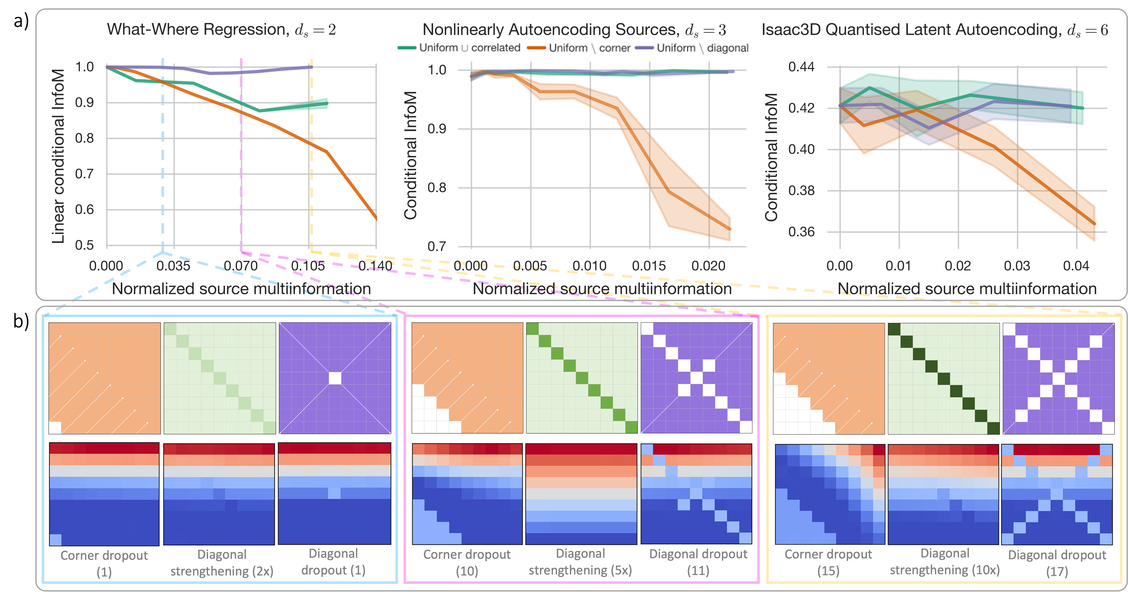
Figure 2: a) We study three tasks of varying source dimensionality $d_{s}$, model complexity, supervision signal, and input data modality (Section 3). For each task, we plot conditional InfoM, a measure of modularity, against normalised source multiinformation (NSI), a measure of the statistical dependencies in the sources. Across the three tasks, we observe that cutting corners severely degrades modularity (orange), whereas equivalently changing the NSI in ways that preserve the rectangular support boundary (green, purple) affects modularity less. Shaded regions denote standard error of the mean. b) For What-Where Regression, we visualise the source distributions at various NSI values (top) as well as the tuning of an example neuron (bottom; vertical: What; horizontal: Where).

Nonlinear autoencoding of sources. Next we study a nonlinear autoencoder trained to autoencode multidimensional source variables. Again we find (Figure 2a middle) that under biological constraints independent source variables ($\text{NSI}=0$) result in modular latents and that source corner cutting (orange) induces far more latent mixing compared to introducing source correlations while preserving rectangular support (green), or removing central data (purple).

Disentangled representation learning of images. Finally, for an experiment involving high-dimensional image data, we turn to a recently introduced state-of-the-art disentangling method, quantised latent autoencoding (QLAE; Hsu et al. [27, 28]). QLAE is the natural machine learning analogue to our biological constraints. It has two components: (1) the weights in QLAE are heavily regularised, like our weight energy loss, and (2) the latent space is axis-wise quantised, introducing a privileged basis with low channel capacity. In our biologically inspired networks, nonnegativity and activity regularisation conspire to similarly structure the representation: nonnegativity creates a preferred basis, and activity regularisation encourages the representation to use as small a portion of the space as possible. We study the performance of QLAE trained to autoencode a subset of the Isaac3D dataset [43]. We find the same qualitative patterns emerge: corner cutting is a more important determinant of mixing than range-independent correlations or the removal of centrally located data (Figure 2a right).

4 Modularisation in Biologically Inspired Recurrent Neural Networks

Compared to feedforward networks, recurrent neural networks (RNNs) are often a much more natural setting for neuroscience. Excitingly, the core ideas of our analysis for linear autoencoders also apply to recurrent dynamical formulations, and similarly extend to experiments with nonlinear networks.

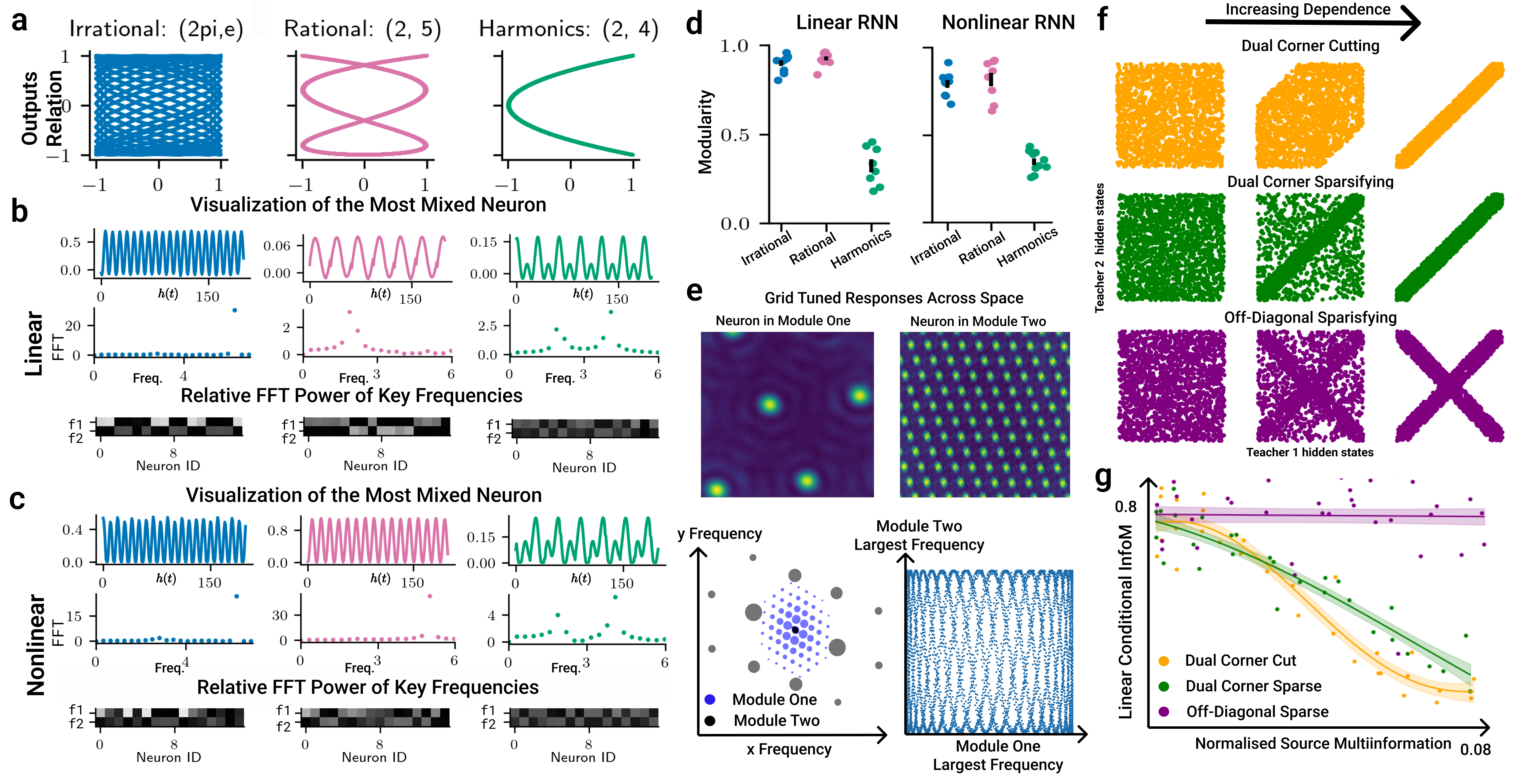
Figure 3: a) Source support visualisations: $\cos(\omega_{1}t)$ vs. $\cos(\omega_{2}t)$. b) The activity of the most mixed neuron in an optimal solution, the same neuron’s Fourier spectrum, and the population’s Fourier spectrum in the two task frequencies show clear modularisation in the irrational and rational cases, and clear mixing the in the harmonic case. c) Same as (b), but with nonlinear RNNs. d) Modularity of RNNs trained on 10 frequency pairs. e) Top: Two optimal grid cells from [14] in different modules. Bottom: The modularisation of these two lattices can be understood from the range-independence of their constituent frequencies, as shown in the joint distribution of the most significant frequency in each module. f) Plot of joint distribution of hidden state activity for two teacher RNNs neurons as we increase the dependence in three different ways. g) Trends of modularity scores of student RNN in three different cases qualitatively agree with our theory.

4.1 Linear RNNs

Linear sinusoidal regression. Linear dynamical systems can only autonomously implement exponentially growing, decaying, or stable sinusoidal functions. We therefore study biologically inspired linear RNNs constrained to model stable sinusoidal signals at certain frequencies:

$${\bm{z}}(t+\delta t)={\bm{W}}_{\mathrm{rec}}{\bm{z}}(t)+{\bm{b}}_{\mathrm{rec}},\quad{\bm{W}}_{\mathrm{out}}{\bm{z}}(t)=\begin{bmatrix}\cos(\omega_{1}t+\phi_{1})\\ \cos(\omega_{2}t+\phi_{2})\end{bmatrix},\quad{\bm{z}}(t)\geq\mathbf{0}.$$ (12)

We study the optimal nonnegative, efficient, recurrent representations, ${\bm{z}}_{t}$, and show that whether the representations of the two frequencies within ${\bm{z}}_{t}$ modularises depends on their ratio. We prove and verify empirically that if one frequency is an integer multiple of the other the encodings mix, whereas if their ratio is irrational they should modularise. Further, we show empirically, and prove in limited settings, that rational non-harmonic ratios should modularise (Appendix C). The intuition for this result is much the same as the linear autoencoding setting: the natural notions of sources are the signals $(\cos(\omega_{1}t),\sin(\omega_{1}t),\cos(\omega_{2}t),\sin(\omega_{2}t))$. Using these sources, we must simply ask: does their support allow for a reduction in activity energy via mixing? In Figure 3a, we visualise the source support for the three prototypical relationships between $\omega_{1}$ and $\omega_{2}$: irrational, rational (but not harmonic), and harmonic. Results of neural network verifications are in Figure 3b (details Appendix G). In the irrational case, the source support is essentially rectangular, so the model modularises. In the harmonic case, large chunks of various corners are missing from the source support, so the model mixes. In the rational case, even though the source support is quite sparse, the corners are sufficiently present such that modularising is still optimal.

Modularisation of grid cells. We now show that these spectral ideas can explain modules of grid cells. Grid cells are neurons in the mammalian entorhinal cortex that fire in a hexagonal lattice of positions [22]. They come in groups, called modules; grid cells within the same module have receptive fields (firing patterns) that are translated copies of the same lattice, and different modules are defined by their different lattice [60]. Current theories suggest that the grid cell system can be modelled as a RNN with activations built from linear combinations of frequencies [14], just like the linear RNNs considered here. Importantly, these grid cell theories use the same biological constraints as in this work and show that modules form because the optimal code contains non-harmonically related frequencies that are encoded in different neurons (Figure 3e top). This modularisation can now be theoretically justified in our framework, since non-harmonic frequencies are range-independent and so should be modularised (Figure 3e bottom).

4.2 Nonlinear RNNs

Mixed sinusoidal regression for nonlinear RNNs. We train nonlinear ReLU RNNs with biologically inspired constraints to perform a frequency mixing task (details Appendix G). We provide a pulse input $P_{\omega}(t)=\mathbb{I}\left[\operatorname{mod}_{\omega}(t)=0\right]$ at two frequencies, and the network has to output the resulting “beats” and “carrier” signals:

$${\bm{z}}(t+\Delta t)=\text{ReLU}\left({\bm{W}}_{\text{rec}}{\bm{z}}(t)+{\bm{W}}_{\text{in}}\begin{bmatrix}P_{\omega_{1}}(t)\\ P_{\omega_{2}}(t)\end{bmatrix}+{\bm{b}}_{\text{rec}}\right),\;\begin{bmatrix}\cos([\omega_{1}-\omega_{2}]t)\\ \cos([\omega_{1}+\omega_{2}]t)\end{bmatrix}={\bm{W}}_{\text{out}}{\bm{z}}_{t}+{\bm{b}}_{\text{out}}.$$ (13)

Results are in Figure 3c. Identical range-dependence properties but applied to the frequencies $\omega_{1}-\omega_{2}$ and $\omega_{1}+\omega_{2}$ determine whether or not the network modularises: irrational, range-independent frequencies modularise; harmonics, with their large missing corners, mix; and other rationally related frequencies are range-dependent but no sufficient corner is missing, so they modularise.

Modularisation in nonlinear teacher-student distillation. To test our predictions of when RNNs modularise, but in settings more realistic than pure frequencies, we generate training data trajectories from randomly initialised teacher RNNs with tanh activation function, and then train student RNNs (with a ReLU activation function) on these trajectories. The student’s representation is constrained to be nonnegative (via its ReLU) and has its activity and weights regularised (see Section G.2 for details). Using carefully chosen inputs at each timestep, we are able to precisely control the teacher RNN hidden state activity (i.e., the source distribution). This allows us to change correlations/statistical independence of the hidden states, while either maintaining or breaking range independence. We consider three settings (Figure 3e). First, when statistical and range independence are progressively broken (in orange). Second, where statistical, and to a lesser extent range, independence gets progressively broken (in green). Third, where only statistical independence gets progressively broken (in purple). We qualitatively observe, as our linear theory predicts, that students learns modular representations when range independence is maintained regardless of the statistical dependence of the teacher RNN hidden states (Figure 3f).

5 Modularisation of Prefrontal Working Memory

We now apply our results to neuroscience to explain a puzzling difference in monkey prefrontal neurons in two seemingly similar working memory tasks. In both tasks [71, 45], items are presented to an animal, and, after a delay, must be recalled according to the rules of the task. Similarly, in both tasks, as well as in neural networks trained to perform these tasks [8, 48, 70], the neural representation during the delay period consists of multiple subspaces, each of which encodes a memory of one of the items. Bizarrely, in one task these subspaces are orthogonal to one another [45], a form of modularisation in the representation of different memories sans a preferred basis, while in the other they are not [71].

In more detail, Xie et al. [71] train monkeys on a sequential working memory task in which the subject observes a sequence of $N$ dots positioned on a screen then, after a delay, must report that same sequence via saccading to the dot locations in order (Figure 4a). They find that the neural representation in the delay period decomposes into $N$ subspaces (one for each item) that are significantly non-orthogonal. (To calculate the alignment we reanalysed the data using a different measure of alignment from the original paper, inspired by Panichello and Buschman [45]. This is because we find other measures to be biased Appendix H). On the other hand, in a related task, Panichello and Buschman [45] (P&B) find orthogonal memory. They present monkeys with two coloured squares, one below the other, then, after a delay, present a cue that tells the monkey to recall the top or bottom colour via a saccade to the appropriate point on a colour wheel (Figure 4c). P&B find that, during the delay after cue presentation, the colours are encoded in two subspaces that are orthogonal to one another (Figure 4d).

Why does one experiment result in orthogonality but the other not? Our theory says that differences in range (in)dependence can lead to modular or mixed (orthogonal or not in this case) codes. Crucially, across trials, P&B sample the two colours independently, whereas Xie et al. [71] sample the dots without replacement. The latter sampling scheme compromises orthogonality since there are corners (indeed an entire diagonal) missing from the source support.

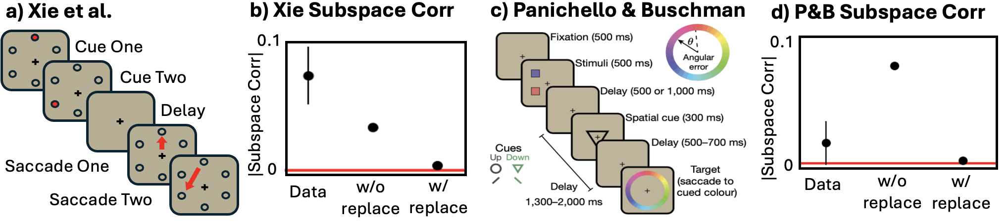
Figure 4: a) Xie et al. [71] task. b) We estimate the non-orthogonality of subspaces in data, and networks trained on sequences sampled with and without replacement or with correlations (Appendices H and I). Sampling without replacement, as in the experiment, gives the best fit. c) Panichello and Buschman [45] task, replicated. d) Subspace correlations for data and models. Sampling with replacement is necessary to fit the data.

We model this in biologically-constrained RNNs for each task. For the Xie et al. [71] task we present two inputs sequentially to a linear RNN with nonnegative hidden state and ask the networks to recall the inputs, in order, after a delay. Interestingly, our results depend on the particular choice of item encoding (one-hot or 2D), in ways that can be understood using our theory (Appendix I). To compare to the prefrontal data, we extract the item encoding from the prefrontal data during the delay period for single-element sequences. For P&B we assume the encoding is 2D.

Our simulated models recapitulate the major observations of monkey prefrontal representations. Sequences sampled without replacement in the Xie et al. [71] task lead to aligned encoding subspaces like data (Figure 4b), while colours sampled independently lead to orthogonal encodings in the P&B task as in data (Figure 4d). Conversely, as a prediction for future primate experiments, swapping the sampling scheme swaps the prediction. That said, there remain some puzzling discrepancies to explore. Panichello & Buschmann find that about 20% of colour-tuned neurons are tuned to the both colours, despite the orthogonal encoding [45], whereas our theory would predict all neurons would respond to one colour. Further, despite a qualitative match (i.e., orthogonal versus non-orthogonal), we do not obtain the exact angles between subspaces in Xie et al. using our RNNs (Figure 4b).

6 Orthogonalisation of Preparatory and Potent Subspaces in Motor Cortex

For our second neuroscience puzzle we turn to the motor cortex. Neural activity in primate motor cortex appears to drive movements, such as reaching. Further, in classic delayed-reach tasks, where the monkey is shown a cue then, after a delay, has to reach towards that cue, there is a delay-period activity that encodes which movement the monkey is preparing to make [33]. This has led researchers to break the motor cortical neural activity into two subspaces: a preparatory neural subspace, in which upcoming movements are prepared, and a potent subspace that actually drives behaviour. RNN models trained on delayed-reach tasks also show preparation related activity. However, while in neural data these two subspaces are orthogonal, in most RNN models the two are aligned [21]. Intriguingly, a further study trained RNNs to perform two cued-reaches rapidly, one after another, and found that then the preparatory and potent subspaces were orthogonal [75]. Why are these subspaces aligned in RNNs trained on single action tasks, but orthogonal in both the brain and networks trained on dual-reach tasks?

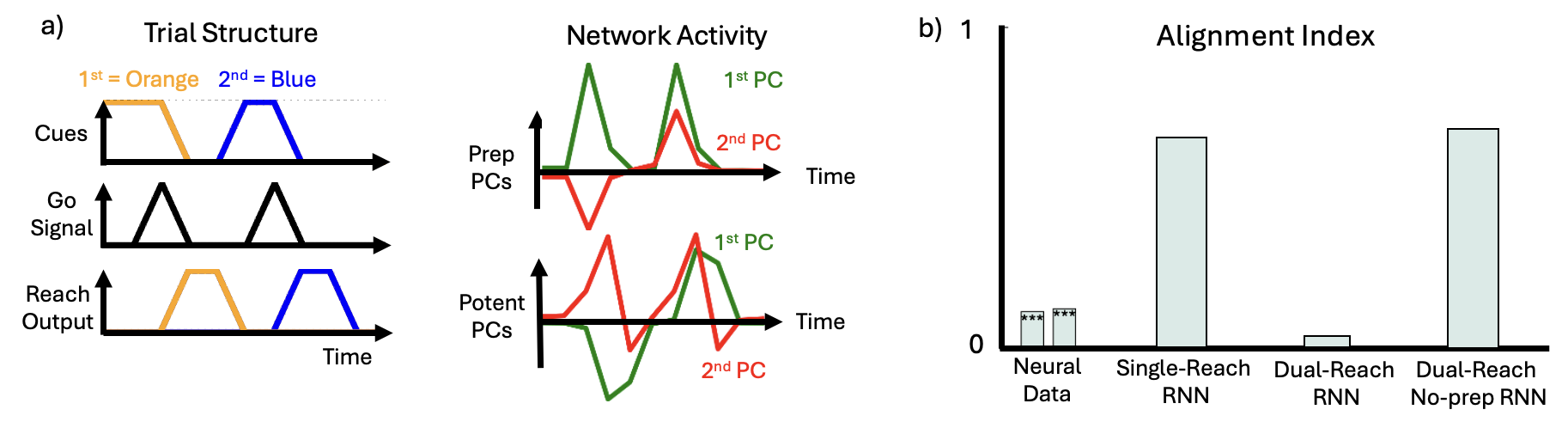
Figure 5: a) Dual-reach task. An RNN receives a cue that says which reach to perform (orange or blue), and a go signal. It must perform the required reach after the go cue. Network activity can be broken down into preparatory directions, which prepare the network to reach in a certain direction, and potent directions, which enact the movement. b) Following [21], we calculate an alignment index: the proportion of preparatory activity during single-reach trials explained by the potent subspace (details in Appendix I). For networks trained to perform only single reaches, the two subspaces are aligned; while for networks trained to perform dual-reach tasks, and neural data, the two are orthogonal. Finally, a network trained to perform two reaches, but in which the preparatory cue for the second movement arrives after the end of the first movement, again has aligned subspaces, matching our theory.

This can be understood in our framework as an independence effect. During the dual-reach, but not the single-reach, task, the preparatory and potent subspaces are both being concurrently used. This ensures that the activity in the two subspaces can be range independent from one another, whereas in the single-reach case either the preparatory or the potent signal is non-zero, but never both. Since independence drives orthogonalisation, this means that only in the dual-task case is there a push towards orthogonalising the representation. We train networks to perform simple analogues of the single- and dual-reach tasks (details Appendix I) and recover the same results as stated: only those trained on dual-reach tasks have close-to-orthogonal potent and preparatory subspaces Figure 5. Finally, this effect only occurs if preparation and movement overlap. If a network is trained on dual-reach tasks in which the second preparatory cue arrives after the end of the first movement, the subspaces again align Figure 5. Motor cortex likely orthogonalises these subspaces since it is regularly performing sequences of movements, preparing the next while performing another. This is natural, but does mean that our predictions are really about the behaviour of RNN models, since no motor cortex is likely to have range-dependent preparatory and potent activity over the course of the animal’s lifetime.

7 Modular or Mixed Codes for Space & Reward

Our last riddle comes from the entorhinal cortex. This brain area has been thought to contain precisely modular neurons, such as the grid cell code for self-position [22], object vector cells that fire at a particular displacement from objects [30], and heading direction cells [63]. Two recent papers examined the influence of rewarded locations on the grid cell code and find differing effects on the modularity of grid cells. Butler et al. [11] find that rewards rotate the grid cells, but preserve their pure spatial coding, while Boccara et al. [7] find that the grid cells warp towards the rewards, becoming mixed-selective to reward and space.

Whittington et al. [69] study this discrepancy and point to the importance of the reward distribution in these two tasks: Boccara et al. [7] fix the positions of the possible rewards during one day, whereas Butler et al. [11] alternate the animals between periods of free-foraging for randomly placed rewards and periods of specific rewarded locations. However, the arguments of [69], which rely on source independence, are insufficient to explain these modularisation effects, as in neither case are reward and position independent; even in the experiments of Butler et al. [11] there are regions of space that are much more likely to be rewarded.

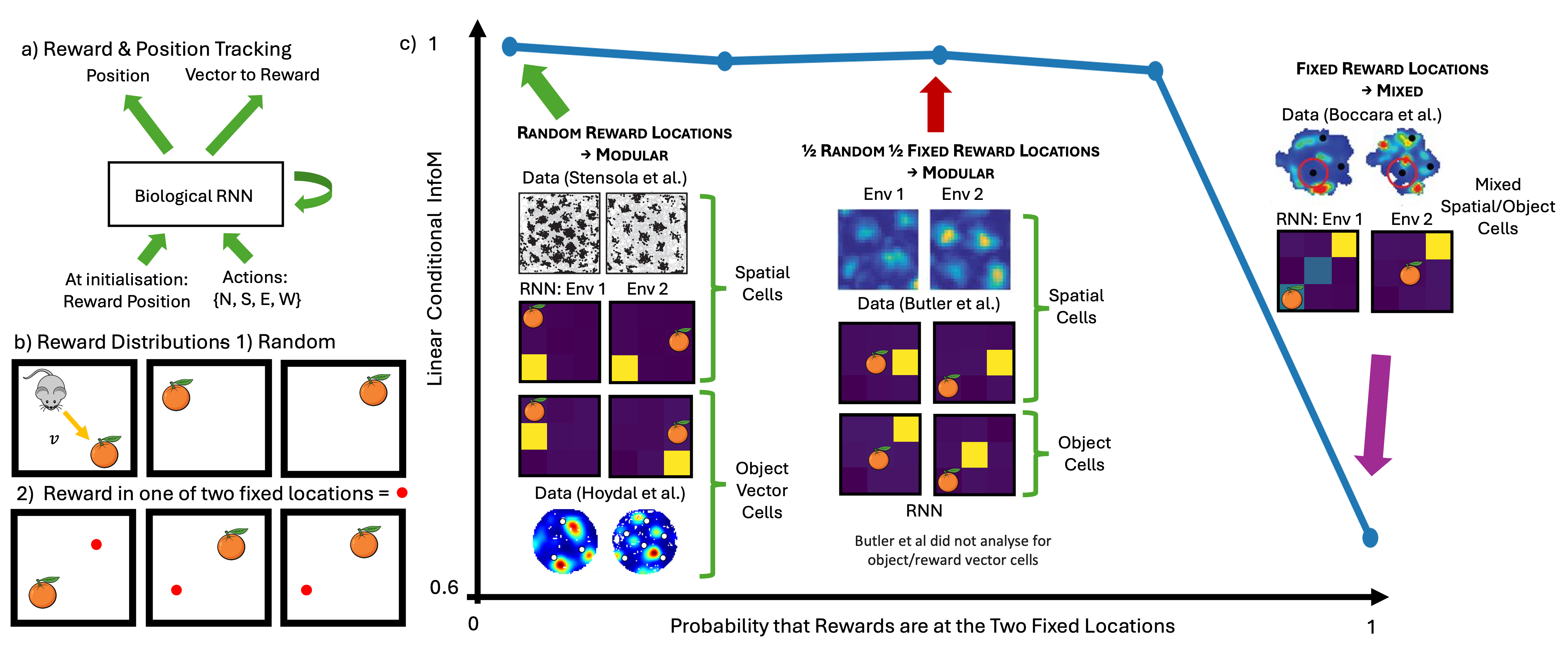
Figure 6: a, b) We train linear RNNs to integrate a sequence of actions to report their current position and displacement from a reward. In some proportion of the rooms, rewards are randomly scattered; in the rest, they are in one of two fixed locations. c) Matching the theory, if some of the rooms are random then reward and position are range-independent, and their representation modularises, as in Stensola et al. [60] or Butler et al. [11]; if in all rooms the rewards occur in one of two fixed locations the representation mixes, with neurons encoding both reward and self position, as in Boccara et al. [7].

However, with our improved understanding of modularisation, this makes sense. Despite Butler et al. [11] correlating reward and position, critically, they leave them range independent—all combinations of reward and position are possible. On the other hand, Boccara et al. [7] make certain combinations of reward and position impossible, making them not just correlated, but range correlated. As such, our theory matches this modularisation pattern. To test this we train a linear biological RNN (details Appendix I) to report both its self-position and displacement from a reward as it moves around an environment (Figure 6). We train RNNs on settings with different relationships between reward and position; for some RNNs the rewards are in fixed positions in every environment (range dependent and statistically dependent), for others reward and position are uniformly random in each room (range independent and statistically independent), and for a final group have both settings in different proportions (range independent but statistically dependent). As we vary the proportion of fixed rooms, we find the optimal representation stays modular, containing separate spatial and reward-vector cells as in Butler et al. [11], until all the sampled rooms have fixed reward positions, at which point neurons become mixed selective to reward and self-position, as in Boccara et al. [7]. As such, our theory now covers all known modularity results about grid cells.

8 The Mixed Origins of Mixed Selectivity

Why neurons might be mixed selective is a matter of debate in neuroscience [3, 65]. Theories of nonlinear mixed selectivity have argued that, analogously to a nonlinear kernel, such schemes permit linear readouts to decode nonlinear task functions of the sources. This is likely a key part of the mixed selectivity found in some brain areas, like the cerebellum [37], mushroom body [1], and perhaps certain prefrontal or hippocampal representations [6, 9]. However, our theory raises the possibility for other explanations of both nonlinear and linear mixed selectivity that do not require tasks including nonlinear functions of the sources.

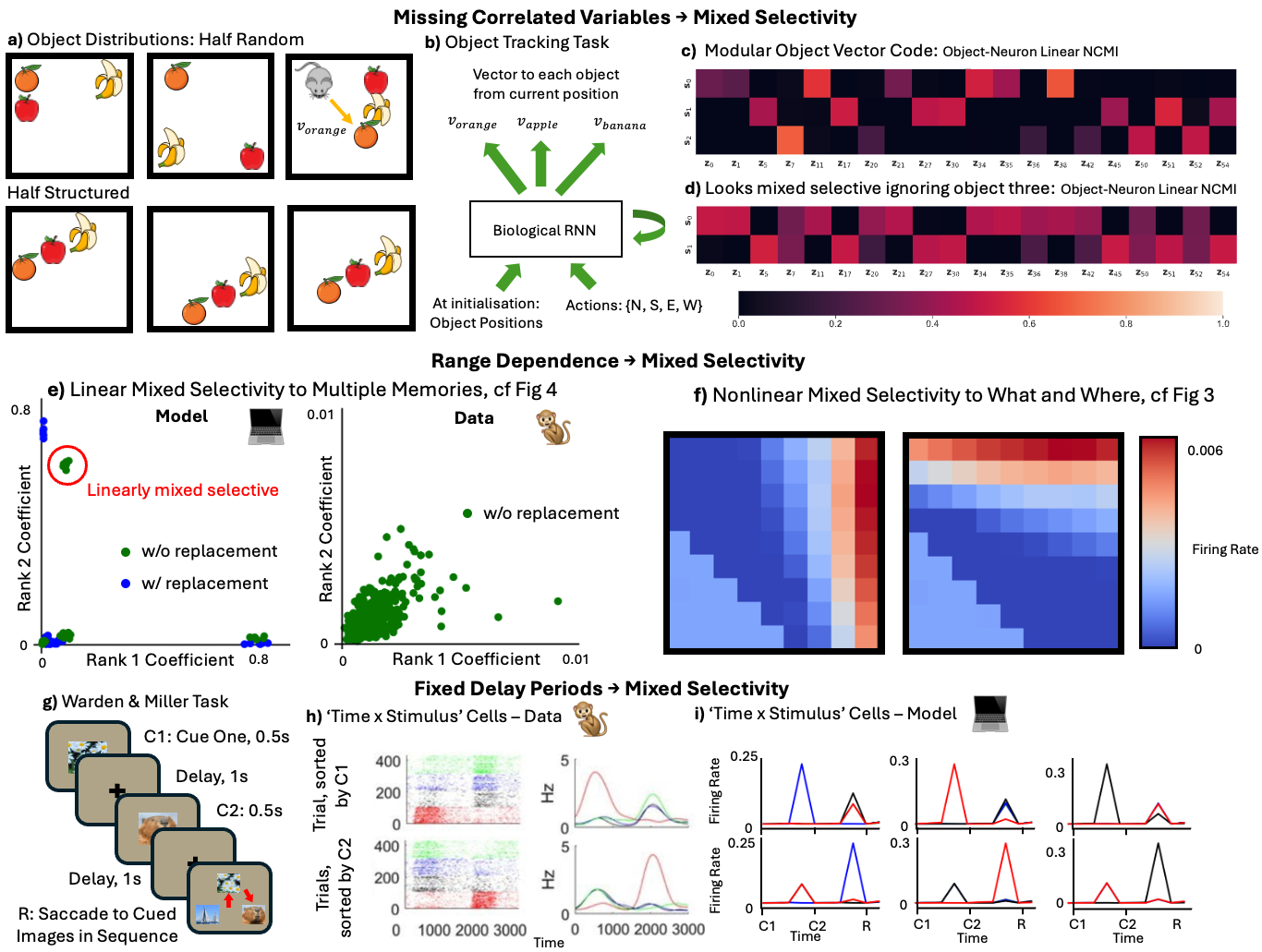
Figure 7: a, b) We train linear RNNs to report displacement to three objects as an agent moves within many rooms. In each room, object instances are either completely random (a, top) or clustered in a random line (a, bottom); object positions are therefore range independent but correlated. c) The neurons are modular: each neuron’s activity is conditionally informative of only a single object given the others. d) However, if an experimenter were only aware of two of the three objects, the neurons that purely encode the disregarded object would appear mixed selective due to the statistical dependencies between objects. e) We extract the tuning of neurons to different memory encodings from both RNNs (left) and neural data (right) [71]. In both the models and data, many neurons are linearly mixed selective. f) In nonlinear, but linearly decoded, representations from the What-Where Regression task, many neurons are nonlinearly mixed selective. g) Warden and Miller [67] train monkeys to see, then report a sequence of two images. Mikkelsen et al. [41] reanalyse the data and find h) neurons tuned to both time and stimulus identity. i) Our linear RNN model recapitulates this.

Missing sources. First, a purportedly mixed selective neuron could actually be a modular encoding, but of a source variable unknown to the experimenter. For example, despite the many modular neurons in entorhinal cortex, there are also many neurons that seem mixed selective to combinations of spatial variables, such as speed, heading direction, or position [23]. An alternate explanation is that these neurons may (in part) be purely selective for another unanalysed variable that is itself correlated with the measured spatial variables or behaviour. We highlight a simple example of this effect in Figure 7a, b. Imagine a mouse is keeping track of three objects as it moves in an environment (Figure 7a); we model this as a linear biological RNN that must report the displacement of all objects from itself (Figure 7b). Object positions are range independent but correlated, so the RNN representation modularises such that each neuron only encodes one object (Figure 7c). However, if an experimenter were only aware of two of the three objects, they would instead analyse the neural tuning with respect to those two objects. Due to the statistical dependencies between object positions, they would find mixed selective neurons that are in reality purely coding for the missing object (Figure 7d).

Range-dependent sources. Second, our theory gives a precise set of inequalities for (biologically constrained) modularisation of scalar sources. Breaking the condition means the optimal representation is linearly mixed selective (Figures 1, 3, 4 and 7). These ideas also qualitatively predict modularisation of nonlinear feedforward and recurrent networks across a range of settings (Figures 2 and 3). Figure 7e, f re-illustrates these results, which suggest that nonlinear mixed selectivity might exist simply to save energy, rather than the typical rationale of permitting flexible linear readouts of arbitrary categorisations [3, 65].

Sequential processing. Finally, multiple works have highlighted nonlinear mixed selectivity to stimulus feature and time within task [46, 12, 13]. We show that simple linear sequential computations can produce this seemingly nonlinear temporal mixed selectivity. For example, Warden and Miller [67] train monkeys to view sequences of two images separated fixed delays (Figure 7g). To be rewarded, monkeys must report the stimuli, e.g., by saccading to the images in the correct sequence. Recently, Mikkelsen et al. [41] reanalysed this data and found that many neurons are nonlinearly mixed selective to stimulus and time (Figure 7h). However, we train a biological linear RNN to recall two sequentially presented one-hot cues separated by delays, and find similar neurons (Figure 7i and Appendix I). This form of nonlinear mixed selectivity arises not from downstream readout pressures, but simply as the optimal energy-efficient code during fixed-length delays. Indeed, interpreting these as nonlinear relies on one viewing time as a scalar linearly increasing variable; if instead time is represented one-hot, both monkey and model neurons could be interpreted as linearly mixed selective.

9 Discussion

In this work we have given precise constraints that cause linear feedforward and recurrent networks under biological constraints to modularise. These constraints are highly dependent on the co-range properties of variables, and have helped us understand patterns of modularisation in both nonlinear networks and the brain.

Theoretical limitations. Our theory predicts binary yes/no modularity in linear sources (each uni-dimensional) with L2 energy constraints, but does not yet predict the modularisation of multidimensional sources, nonlinear settings, other norms (using an L1 sparsity penalty on neural activity has a long history [44]), nor does it prescribe the degree of modularity (rather than perfectly modular or not). These could all be useful extensions.

Mixed selectivity. In neuroscience our findings add nuance to the ongoing debate over mixed vs. modular neural coding. Our theory points to a variety of settings in which mixed-selectivity arises under energy constraints, without the requirement of a flexible linear readout for nonlinear classifications that is often argued to the the source of mixed-selectivity. Nevertheless we think that flexible linear readouts are sometimes the source of mixed-selectivity, to allow kernel regression-like classification. We expect this is true for neurons in the cerebellum or mushroom body, as well as the some cortical neurons that have non-linearly mixed selective coding of independent variables—something our theory would never predict [6]. Yet our theory suggests several alternative explanations for mixed-selectivity that seem plausible for many recorded neural populations, for example those in entorhinal (Figure 6) and prefrontal cortex (Figure 4) including the dataset for which these nonlinear classification theories were originally developed [67].

Neural limitations. Our theory prescribes when biological neural populations should be modular or not, yet some of the PFC (Section 5) and motor cortex (Section 6) data we explain is when the population is orthogonal or not. Orthogonal is not necessarily modular; indeed some real individual neurons are seemingly not fully modular, contrary to our theory. This may be a shortcoming of our simple theory. However, it also possible that it is best to understand these mixed-selective neurons, for example in Panichello and Buschman [45]’s task, as a different computational population. This feature—pure and mixed selective cells playing different computational roles—is observed in entorhinal cortex: pure grid cells code only for spatial position while conjunctive grid/heading-direction cells [54] are thought to be critical in integrating velocity to update the position code [66] (much like the analogous heading-direction update neurons in the protocerebral bridge of the fly central complex [64]). We anticipate that incorporating computational elements into our theory will further account for mixed selective neurons in frontal cortex and beyond.

Disentangling what? In machine learning, our work bolsters the importance of range properties over statistical independence in the disentanglement literature. On this we agree with Roth et al. [52], who argue that range independence is the more meaningful form of independence. Further, our conditions have qualitative similarities to sufficient spread conditions from the matrix factorisation literature [61, 62], perhaps suggesting a deeper correspondence. It is intriguing that the constraints inspired by those in biology, which have shown promise for disentangling [69], and have links to state-of-the-art disentangling methods [27, 28], are sensitive to just this form of independence.

Reproducibility

Code used in producing this work is available at https://github.com/kylehkhsu/dont-cut-corners/.

Appendix A Related Works

Machine learning. The disentangled representation learning community has found inductive biases that lead networks to prefer modular or disentangled representations of nonlinear mixtures of independent variables. Examples include sparse temporal changes [35], smoothness or sparseness assumptions in the generative model [74, 25], and axis-wise latent quantisation [27, 28]. Relatedly, studies of tractable network models have identified a variety of structural aspects, in either the task or architecture, that lead to modularisation, including learning dynamics in gated linear networks [55], architectural constraints in linear networks [32, 58], compositional tasks in linear hypernetworks and nonlinear teacher-student frameworks [56, 39], or task-sparsity in linear autoencoders [20].

Neuroscience. Theories prompted by the recognition of neural mixed-selectivity in biological networks have argued that these nonlinearly mixed selective codes might exist to enable a linear readout to flexibly decode any required categorisation [50], suggesting a generalisability-flexibility tradeoff between modular and nonlinear mixed encodings [6]. Modelling work has studied task-optimised network models of neural circuits, some of which have recovered mixed encodings [42]. However, other models trained on a wide variety of cognitive tasks have found that networks contain meaningfully modularised components [73, 15, 17]. Dubreuil et al. [16] study recurrent networks trained on similar cognitive tasks and find that, depending on the task structure, neurons in the trained networks can be grouped into populations defined by their connectivity patterns. To this developing body, our work and its predecessor [69] present understanding of when simple biological constraints would encourage encodings of many variables to be modularised into populations of single pure-tuned variables, or when mixed-selectivity would be preferred. Compared to [69] which only works when source variables are statistically independent, our work determines modularity for (almost) any dataset even when source variables are not independent. This is a dramatically more complete understanding of the boundary between mixed and modular codes that allows us to understand behaviour in both biological and artificial neurons that previously eluded explanation.

Independent components analysis and matrix factorization. Our linear autoencoding problem (Theorem 2.1) bears some similarity to linear independent components analysis (ICA) and matrix factorization (MF). These assume data ${\bm{y}}_{i}$ is linearly generated from a set of constrained sources, ${\bm{y}}_{i}={\bm{A}}{\bm{s}}_{i}$, and build algorithms to recover ${\bm{s}}_{i}$ from ${\bm{y}}_{i}$. The literature studies different combinations of (1) assumptions on the sources ${\bm{s}}_{i}$, e.g. independence [5], nonnegativity[49], or boundedness [31]; (2) assumptions on the mixing matrix ${\bm{A}}$, e.g. nonnegative in nonnegative matrix factorisation and (3) algorithms, often deriving identifiability results: conditions that the data must satisfy for a given algorithm to succeed. Some work even derives biological implementations of such factorisation algorithms [47, 10]. In our work we study the conditions under which a particular biologically inspired representation modularises a set of bounded sources. We provide conditions on the sources under which the optimal representation is modular, morally similar to identifiability results (indeed, other identifiability results, like ours, sometimes take the form of sufficient spread conditions [61, 62]). We differ from previous work in the representation we study (which has only been studied before by [69]), the form of our identifiability result (which is both necessary and sufficient, has not been derived before, and assumes only that the sources are bounded), and that these developments allows us to explain both recurrent modularisation and neural data.

Appendix B Optimal Representations in Positive Linear Autoencoders

We develop our results in three parallel ways. First, in Section B.1, we study simple two source problems and pedagogically derive our results. Second, in  Section B.2, we state the full inequality constraints, Theorem 2.1, and formally prove them using the same type of argument as in the pedagogical approach. Finally, in Section B.4, we study the more general setting of invertible linear mixtures of sources and use a third, pertubative, approach to derive more general conditions under which a modular solution is a local optima. These conditions recover our main inequalities as a special case, but in a slightly weaker format, as they only guarantee the local optimality of modular solutions, unlike our main results. The three presentations of the result are independent, and readers may choose whichever they find more palatable. Then, in Section B.3, we prove the corollary corollary 2.3. Finally, in Section B.5, we show the equivalence between the two characterisations of the condition, via either the set of inequalities or the convex hull.

B.1 Intuitive Development for Two Sources

B.1.1 Problem Statement

To begin, we study our simplest setting: a positive linear autoencoder that has to represent two bounded, scalar, mean-zero, sources, $x^{[i]}$ and $y^{[i]}$. These are encoded in a representation ${\bm{z}}^{[i]}\in\mathbb{R}^{N}$, where $N$ is the number of neurons, which we will always assume to be as large as we need it to be, and in particular larger than the number of encoded variables. Our first constraint is given by the architecture. The representation is a linear function of the inputs plus a constant bias, and you must be able to decode the variables from the representation using an affine readout transformation:

$${\bm{z}}^{[i]}={\bm{W}}_{\text{in}}\begin{bmatrix}x^{[i]}\\ y^{[i]}\end{bmatrix}+{\bm{b}}_{\text{in}}\qquad{\bm{W}}_{\text{out}}\cdot{\bm{z}}^{[i]}+{\bm{b}}_{\text{out}}=\begin{bmatrix}x^{[i]}\\ y^{[i]}\end{bmatrix}$$ (14)

Where ${\bm{W}}_{\text{in}}$ and ${\bm{b}}_{\text{in}}$ are the readin weight matrix and bias, and ${\bm{W}}_{\text{out}}$ and ${\bm{b}}_{\text{out}}$ are the readout weight matrix and bias.

Our second constraint, inspired on the one hand by the non-negativity of biological neural firing rates, and on the other by the success of the ReLU activation function, is the requirement that the representation is non-negative: ${\bm{z}}^{[i]}\geq{\bf 0}$.

Subject to these constraints we optimise the representation to minimise an energy-use loss:

$$\mathscr{L}=\frac{1}{D}\sum_{i=1}^{D}||{\bm{z}}^{[i]}||^{2}+\lambda(||{\bm{W}}_{\text{out}}||^{2}_{F}+||{\bm{W}}_{\text{in}}||_{F}^{2})=\langle||{\bm{z}}^{[i]}||^{2}\rangle_{i}+\lambda(||{\bm{W}}_{\text{out}}||^{2}_{F}+||{\bm{W}}_{\text{in}}||_{F}^{2})$$ (15)

This loss is inspired on the one hand by biology, in particular by the efficient coding hypothesis [2, 4] and its descendants. These theories argue that neural firing should perform its functional role (e.g. encoding information) maximally energy-efficiently, for example by using the smallest firing rates possible, and has been used to understand neural responses across tasks, brain areas, individuals, and organisms [38, 57]. Our loss can be seen as a slight generalisation of this idea, by minimising energy use both through firing rates and through synapses [24]. On the other hand, this loss is similar to weight decay, a widely used regularisation technique in machine learning, that has long been linked to a simplicity bias in neural networks [36].

Our question can now be simply posed. What properties of the sources $x^{[i]}$ and $y^{[i]}$ ensure that they are optimally represented in disjoint sets of neurons? Equivalently, when does the representation modularise? The arguments of Whittington et al. [69] can be used to show that if the two sources are statistically independent they should optimally modularise. We will find a much weaker set of conditions are necessary and sufficient for modularisation. In particular, we derive precise conditions on the range of allowed $(x,y)$ pairs that ensures modularising is optimal. For example, we will show that if the sources are range-symmetric ($|\min_{i}x^{[i]}|=\max_{i}x^{[i]}$) and extreme point independent, meaning $\min_{i}(x^{[i]}+y^{[i]})=\min_{i}x^{[i]}+\min_{i}y^{[i]}$, they should modularise.

The structure of our argument goes as follows, by assumption the representation is a affine transformation of the inputs:

$${\bm{z}}^{[i]}={\bm{u}}x^{[i]}+{\bm{v}}y^{[i]}+{\bm{b}}$$ (16)

We will show that, for any fixed encoding sizes $||{\bm{v}}||$ and $||{\bm{u}}||$, the weight loss ($||{\bm{W}}_{\text{out}}||_{F}^{2}+||{\bm{W}}_{\text{in}}||_{F}^{2}$) is minimised by orthogonalising ${\bm{v}}$ and ${\bm{u}}$, in particular, by modularising the representation. We will then derive the conditions under which, for fixed encoding size, the activity loss is minimised by modularising the representation. If, whatever the encoding sizes, both losses are minimised by modularising, and the activity loss is minimised only by modularising (i.e. there are no other solutions that are equally good), the optimal representation is modular. Conversely, if the activity loss is not minimised by modularising, then you can always decrease the loss by slightly mixing the representation, hence the optimal representation is mixed.

B.1.2 Conditions for Modularisation

For simplicity we will make the following assumptions, that will be relaxed later:

1. The sources are linearly uncorrelated, $\langle x^{[i]}y^{[i]}\rangle_{i}=\frac{1}{D}\sum_{i=1}^{D}x^{[i]}y^{[i]}=0$

2. The sources are range-symmetric around zero, i.e. $|\min_{i}x^{[i]}|=\max_{i}x^{[i]}$ and $|\min_{i}y^{[i]}|=\max_{i}y^{[i]}$

We will consider the two losses in turn.

B.1.3 Weight Loss

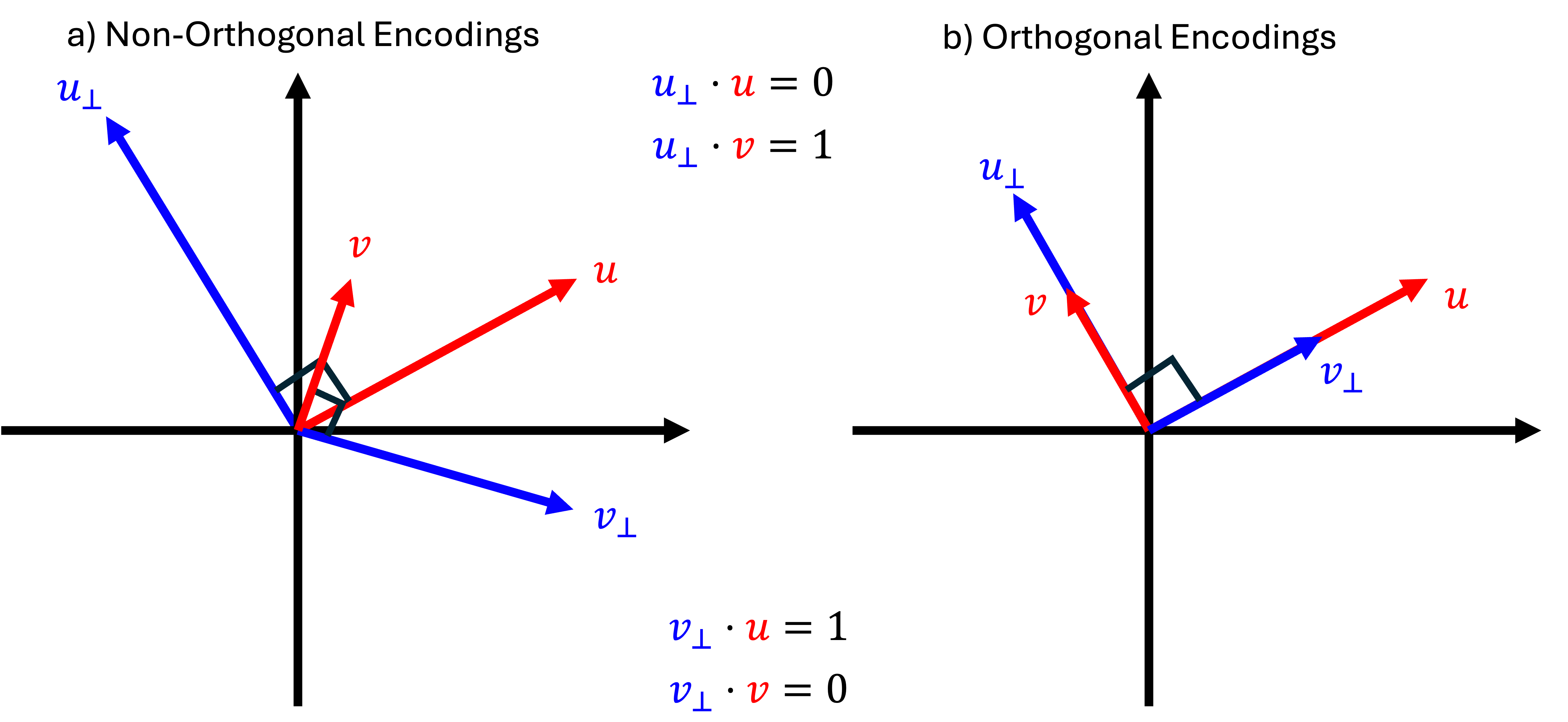
Figure 8: Schematics showing that modular representations minimise readout weight energy, $||W_{\text{out}}||_{F}^{2}$, independent of encoding size. Aligning the encoding vectors (a) necessarily requires longer pseudoinverse vectors than an orthogonal solution (b), for example a modular solution.

First, for a given linear representation of the form in equation 16, the minimum squared norm readout matrix has the following form:

$${\bm{W}}_{\text{out}}=\begin{bmatrix}{\bm{v}}_{\perp}^{T}\\ {\bm{u}}_{\perp}^{T}\end{bmatrix}$$ (17)

Where ${\bm{v}}\perp$ and ${\bm{u}}_{\perp}$ are the two vectors in the span of ${\bm{u}}$ and ${\bm{v}}$ with the property that ${\bm{v}}_{\perp}^{T}{\bm{v}}=0$ and ${\bm{v}}_{\perp}^{T}{\bm{u}}=1$, and the equivalent conditions for ${\bm{u}}_{\perp}$ (as in figure 8). To convince yourself of this consider the fact that these are the only two vectors in this plane that will produce the desired output, and you could add off-plane components to them, but that would only increase the weight loss for no gain, since:

$$||{\bm{W}}_{\text{out}}||_{F}^{2}=\operatorname{Tr}[{\bm{W}}_{\text{out}}{\bm{W}}_{\text{out}}^{T}]=||{\bm{u}}_{\perp}||^{2}+||{\bm{v}}_{\perp}^{2}||$$ (18)

These vectors, ${\bm{v}}\perp$ and ${\bm{u}}_{\perp}$, are the rows of the psuedoinverse, so henceforth we shall call these vectors the pseudoinverse vectors.

Then, with $\theta$ denoting the angle between ${\bm{v}}$ and ${\bm{u}}$, the readout loss can be developed using simple trigonometry:

$$||{\bm{W}}_{\text{out}}||^{2}_{F}=||{\bm{v}}_{\perp}||^{2}+||{\bm{u}}_{\perp}||^{2}=\frac{1}{\sin^{2}(\theta)}\bigg{(}\frac{1}{||{\bm{u}}||^{2}}+\frac{1}{||{\bm{v}}||^{2}}\bigg{)}$$ (19)

This has two interpretable properties. First, the larger the encoding the smaller the weight cost, and, second, the more aligned the two encodings the larger the weight cost. Both make a lot of sense, the more teasing apart of the representation is needed to extract the variable, the larger the weights, and the higher the loss. One claim we’ll use later is that, for a given encoding size $||{\bm{u}}||$ and $||{\bm{v}}||$, all solutions with ${\bm{u}}^{T}{\bm{v}}=0$ are equally optimal. In particular, this is true of the modular solution:

$${\bm{u}}=\begin{bmatrix}{\bm{u}}^{\prime}\\ {\bf 0}\end{bmatrix}\quad{\bm{v}}=\begin{bmatrix}{\bf 0}\\ {\bm{v}}^{\prime}\end{bmatrix}$$ (20)

Thus far we’ve discussed was the output weight cost. The input weight norm is even simpler:

$$||{\bm{W}}_{\text{in}}||_{F}^{2}=||\begin{bmatrix}{\bm{u}}&{\bm{v}}\end{bmatrix}||_{F}^{2}=\operatorname{Tr}[{\bm{W}}_{\text{in}}^{T}{\bm{W}}_{\text{in}}]=||{\bm{u}}||^{2}+||{\bm{v}}^{2}||$$ (21)

So, for a fixed encoding size, i.e. fixed $||{\bm{u}}||^{2}$ and $||{\bm{v}}||^{2}$, this loss is actually fixed. It therefore won’t effect the optimal alignment of the representation.

Therefore we find, as advertised, that the weight loss is minimised by a modular solution.

B.1.4 Activity Loss and Combination

We now turn to the activity loss and study when it is minimised by modularising. We will play the following game. Let’s say you have a non-modular, mixed, representation; i.e. a representation in which at least one neuron has mixed tuning to both $x$ and $y$:

$$z_{n}^{[i]}=u_{n}x^{[i]}+v_{n}y^{[i]}+\Delta_{n}$$ (22)

Where, $\Delta_{n}=-\min_{i}[u_{n}x^{[i]}+v_{n}y^{[i]}]$ is the minimal bias required to make the representation non-negative. We will find the conditions under which, depending on the mixing coefficients ($u_{n}$ and $v_{n}$), you decrease the loss by forming the modular solution:

$${\bm{z}}_{n}^{[i]}=\begin{bmatrix}u_{n}x^{[i]}\\ v_{n}y^{[i]}\end{bmatrix}-\begin{bmatrix}|u_{n}|\min_{i}x^{[i]}\\ |v_{n}|\min_{i}y^{[i]}\end{bmatrix}=\begin{bmatrix}u_{n}x^{[i]}\\ v_{n}y^{[i]}\end{bmatrix}+\begin{bmatrix}|u_{n}|b_{x}\\ |v_{n}|b_{y}\end{bmatrix}$$ (23)

Where $b_{x}=-\min_{i}x^{[i]}$ is the bias required for a modular encoding of $x^{[i]}$. If, for a given $x^{[i]}$ and $y^{[i]}$, it is true that modularising decreases the loss for all mixings ($u_{n}$ and $v_{n}$) then the modular representation has the optimal energy loss. If there are conditions when modularising increases the loss, then you can always usefully demodularise the representation to decrease the activity loss, and we’ll find that the optimal solution is not perfectly modular.

Let’s analyse the activity loss of these two representations, for the modular representation (eq: 23):

$$\mathscr{L}_{G}^{M}=u_{n}^{2}(\langle(x^{[i]})^{2}\rangle_{i}+b_{x}^{2}))+v_{n}^{2}(\langle(y^{[i]})^{2}\rangle+b_{y}^{2})$$ (24)

And compare it to the mixed (De-modularised) solution:

$$\mathscr{L}_{G}^{D}=u_{n}^{2}\langle(x^{[i]})^{2}\rangle_{i}+v_{n}^{2}\langle(y^{[i]})^{2}\rangle_{i}+\Delta_{n}^{2}$$ (25)

Mixing is prefered over modularity, for a given $u_{i}$ and $v_{i}$, when:

$$(\min_{i}[u_{n}x^{[i]}+v_{n}y^{[i]}])^{2}=\Delta_{n}^{2}<u_{n}^{2}b_{x}^{2}+v_{n}^{2}b_{y}^{2}=u_{n}^{2}\min_{i}(x^{[i]})^{2}+v_{n}^{2}\min_{i}(y^{[i]})^{2}$$ (26)

Let’s get some intuition for what this is saying. Take the simple setting when $v_{n}\approx 0$, i.e. we’re considering a mixed neuron that mainly codes for $x$, with a little bit of $y$. Then two equivalent modular neurons are worse than this hypothetical mixed neuron if, to second order in $v_{n}$, $\Delta_{n}<|u_{n}|b_{x}+\frac{v_{n}^{2}b_{y}^{2}}{|u_{n}|b_{x}}$. Since $\Delta_{n}$ is the mixed bias, this means that mixing a small amount of $y$ into the representation of $x$ is preferable when doing so effectively does not increase the required bias, relative to the bias for only encoding $x$ ($|u_{n}|b_{x}$). For this to be true $u_{n}x^{[i]}$ must have the same minima as $u_{n}x^{[i]}+v_{n}y^{[i]}$. For small enough $v_{n}$, an equivalent phrasing of this condition is that at the times at which $u_{n}x^{[i]}$ takes its minimal value, $y^{[i]}$ is non-negative.

Figure 9: Visualising constraints via corner-cutting. Left: The optimal representation will prefer a mixture containing a small amount of $y$ over modularised if any of the orange shaded regions are missing from the co-range of $x$ and $y$. Right: Drawing these lines for all mixings creates a set of infinitely many lines, each corresponds to the data that must be missing for a particular mixed neuron to be preferable to the equivalent modular solution.

We can visualise this conditions by plotting the allowed range of $x^{[i]}$ and $y^{[i]}$, Figure 9. In grey is the bounding box given by the minima and maxima of $x$ and $y$. Assume for now that $u_{n}$ and $v_{n}$ are positive. For a fixed small value of $v_{n}$ the minima of $u_{n}x^{[i]}+v_{n}y^{[i]}$ remains $u_{n}\min_{i}x^{[i]}$ if there are no datapoints below the line $u_{n}\min_{i}x^{[i]}=u_{n}x+v_{n}y$. Drawing this onto the square, this means there are no datapoints below the red line, in the bottom-left orange region. If this condition is met the representation should mix because this mixed neuron (given by the particular $u_{n}$ and $v_{n}$ ratio) is better than an equivalent modular solution.

That was for positive $u_{n}$ and $v_{n}$. If either of them are negative then you draw a different line corresponding to that sign combination, e.g.: $u_{n}\min_{i}x^{[i]}=|u_{n}|x-|v_{n}|y$. This produces the top-left red line and orange area, again, if there are no datapoints in this shaded region a mixed neuron with mixture coefficients, $|u_{n}|$ and $-|v_{n}|$ is better than the equivalent modular solution. Repeating this for the other sign combinations fills in the other four corners. Hence, we find that a mixed solution in which a small amount of $y$ is mixed into a neuron encoding $x$ is better when there are no datapoints in any of the four corner regions.

That was for one particular pair of $u_{n}$ and $v_{n}$, this hypothetical mixed neuron that encodes mainly $x$ with a pinch of $y$. But to be optimal the modular solution has to be better than all possible mixed neurons. As such we get a family of such constraints: for each mixing of the sources we get a different inequality on the required bias, as described by equation 26. Each of these can be similarly visualised as a corner missing from the co-range of $x$ and $y$, the blue lines in Figure 9 right. If any one of these corners is missing from the co-range of $(x,y)$ then the mixed solution is better, else the modular solution is preferred. We can already see the shape of the ellipse emerging that will be the basis of our later version of the theorem, see Section B.5.

B.1.5 Combining two Analyses

We studied the two loss terms separately, how do they interact?

If the inequality conditions, Equation 26, are satisfied, then the activity loss prefers a modular solution over all mixed representations with the same fixed encodings sizes, $||{\bm{v}}||$ and $||{\bm{u}}||$. Further, the weight loss is also minimised, for a fixed encoding size, by modularising. Therefore the optimal solution will be modular.

Conversely, if one of the inequalities is broken then the activity loss is not minimised at the modular solution. We can move towards the optimal mixed solution by creating a new mixed encoding neuron with infinitesimally low activity, and mixed in proportions given by the broken inequality. This neuron can be created by taking small pieces of the modular encoding of each source, in proportion to the mixing. Doing this will decrease the activity loss. Further, the weight loss is minimised at the modular solution, so, to first order, moving away from modular solution doesn’t change it. Therefore, for each modular representation, we have found a mixed solution that is better, so the optimal solution is not modular. Therefore, if one of the inequalities is broken, the optimal representation will be mixed.

B.1.6 Relaxing Assumptions

We now show how the modularisation behaviour of variables that break the two assumptions listed in B.1.2 can be similarly understood.

Correlated Variables

Correlated variables are easy to deal with, they simply introduce an extra term into the difference in activity losses, equation 25 minus equation 24:

$$\mathscr{L}_{G}^{\text{Modular}}-\mathscr{L}_{G}^{\text{Mixed}}=u_{n}^{2}b_{x}^{2}+v_{n}^{2}b_{y}^{2}-2u_{n}v_{n}\langle x^{[i]}y^{[i]}\rangle_{i}-\Delta_{n}^{2}$$ (27)

This leads to a slightly updated inequality, the solution mixes if:

$$\Delta_{n}<\sqrt{u_{n}^{2}b_{x}^{2}+v_{n}^{2}b_{y}^{2}-2v_{n}u_{n}\langle x^{[i]}y^{[i]}\rangle_{i}}$$ (28)

Figure 10: Visualising how correlations change corner-cutting. Left: It is energetically costly to align the encodings of positively correlated variables

The effect of this change is to shift the corner-cutting lines that determine whether a modular of mixed solution is optimal. This can be understood intuitively. If the variables are positively correlated then positively aligning their representations is energetically costly, and negatively aligning them is energy saving. This is most simply seen in one line of maths. The energy cost contains the following term:

$$\langle({\bm{u}}x^{[i]}+{\bm{v}}y^{[i]})^{2}\rangle_{i}=||{\bm{u}}||^{2}\langle(x^{[i]})^{2}\rangle_{i}+||{\bm{v}}||^{2}\langle(y^{[i]})^{2}\rangle_{i}+{\bm{u}}^{T}{\bm{v}}\langle x^{[i]}y^{[i]}\rangle_{i}$$ (29)

So if the correlation is positive, ${\bm{u}}^{T}{\bm{v}}$ should be negative to decrease the energy, i.e. the encodings should be anti-aligned. Hence, correlated variables have a preferred orientation.

Similarly, the corner cutting has an associated ‘direction of alignment’. If the bottom left corner is missing that means that building a neuron whose representation is a mix of positively aligned $x$ and $y$ is preferable, as it has a smaller minima, requiring less bias. Similarly if the bottom right corner is missing the representation can take advantage of that by building neurons that encode $x$ negatively and $y$ positively, i.e. anti-aligning them.

If these two directions, one from the correlations and one from the range-dependent positivity effects, agree, then it is ‘easier’ to de-modularise, i.e. less of a corner needs to be missing from the range to de-modularise. Conversely, if they mis-align it is harder. This is why the correlations shift the corner-cutting lines up or down depending on the corner. We can see this in figure Figure 10, when the variables are positively correlated it becomes ‘easier’ to mix in the anti-aligned corners, at bottom-right or top-left, and harder at the aligned pair, while the converse is true of the negatively correlated example.

Of interest is a result we can find that guarantees modularisation regardless of the correlation. For these bounded variables the covariances, $\langle x^{[i]}y^{[i]}\rangle_{i}$, are themselves bounded. The most postively co-varying two variables can be is to be equal, then the covariance becomes the variance. Further, the bounded, symmetric, mean-zero variable with the highest variance spends half its time at its max, and half at its min. Similar arguments but with a minus sign for the most anti-covarying representations tell us that:

$$-b_{y}b_{x}\leq\langle x^{[i]}y^{[i]}\rangle_{i}\leq b_{x}b_{y}$$ (30)

These results are similar to those in Hössjer and Sjölander [26]. Putting this into Equation 28, the maximal bounding bias for the most positively or negatively correlated variables to prefer modularising:

$$\Delta_{n}>|u_{n}|b_{x}+|v_{n}|b_{y}$$ (31)

This bound is the development of equation 28 in two cases. First in the maximally positively correlated case when the sign of $u_{i}$ and $v_{i}$ are opposite. Second in the maximally negatively correlated case where the coefficient signs are the same.

From this we can derive the following interesting result, the pedagogical version of Theorem B.1. We will say that if, across the dataset, when $x^{[i]}$ takes its maximum (or minimum) value, $y^{[i]}$ takes both its maximum and minimum values for different datapoints, the two variables are extreme point independent. Another way of saying this is that there is non-zero probability of each of the corners of the rectangle. Now, no matter the value of the correlation, extreme point independence variables should modularise. This is because:

$$\Delta_{n}=-\min_{i}\bigg{[}u_{n}x^{[i]}+v_{n}y^{[i]}\bigg{]}=-|u_{n}|\min_{i}x^{[i]}-|v_{n}|\min_{i}y^{[i]}=|u_{n}|b_{x}+|v_{n}|b_{y}$$ (32)

Hence, we find that even the loosest inequality possible, eqaution 31, is never satisfied. Further, since the variables are extreme point independent their covariance never achieves the equalities in equation 30, so inequality 31 is not satisfied and the variables should modularise.

This means that symmetric extreme point independent variables should always modularise, regardless of how correlated they are. Conversely, for variables that are not quite extreme point independent (perhaps they are missing some corner), there is always a value of their correlation that would de-modularise them.

Range Asymmetric Variables

Thus far we have assumed $|\min_{i}x^{[i]}|=\max_{i}x^{[i]}$, for simplicity. This is not necessary. If this is not the case than there is a ‘direction’ the variable wants to be encoded. Consider encoding a single variable either positively ($z_{+}^{[i]}=|u|x^{[i]}+b$) or negatively ($z_{-}(t)=-|u|x^{[i]}+b$), the losses will differ:

$$\langle(z_{+}^{[i]})^{2}\rangle_{i}=|u|^{2}\big{(}\langle(x^{[i]})^{2}\rangle_{i}+(\min_{i}x^{[i]})^{2}\big{)}\qquad\langle(z_{-}^{[i]})^{2}\rangle_{i}=|u|^{2}\big{(}\langle(x^{[i]})^{2}\rangle_{i}+(\max_{i}x^{[i]})^{2}\big{)}$$ (33)

This is simply expressing the fact that if a variable is mean-zero but asymmetrically bounded then more of the data must be bunched on the smaller side, and you should choose the encoding where most of this data stays close to the origin.

Now, assume without loss of generality that for each variable $b_{x}=|\min_{t}x(t)|\leq\max_{t}x(t)$. Then the identical argument to before carries through for the modularisation behaviour around the lower left corner. Around the other corners however, things are more complicated. There might be a corner missing from the lower right quadrant, but to exploit it you would have to build a mixed neuron that is positively tuned to $y$ but negatively tuned to $x$. This would incur a cost, as suddenly the $x$ variable is oriented in its non-optimal direction. Therefore the calculation changes, because the modular solution can always choose to ‘correctly’ orient variables, so doesn’t have to pay this cost. This is all expressed in the same inequalities, eqn. 28:

$$\Delta_{n}<\sqrt{u_{n}^{2}b_{x}^{2}+v_{n}^{2}b_{y}^{2}-2v_{n}u_{n}\langle x^{[i]}y^{[i]}\rangle_{i}}$$ (34)

This effect can also be viewed in the required range plots, where it translates to a much larger corner being cut off in order to pay the cost of switching around the variables.

Figure 11: Visualising how asymmetric ranges change corner-cutting. When the ranges are asymmetric much larger corners must be cut off the ‘longer’ sides before mixing becomes preferable to modularising.

One quick point is that, for range assymetric variables, the covariance is unbounded, and so it can be large enough to demodularise any pair of variables. Assume for demonstration you have two variables with the same max and min ($b_{\max}$ and $b_{\min}$). The highest covariance you can reach with this pair of bounded, mean-zero, variables is for both variables to spend most of their time either both at the top of their range with some probability $p$, or at the bottom with some probability $1-p$. Because the variables are mean-zero $b_{\max}p=-b_{\min}(1-p)$. Now the covariance is $b_{\min}^{2}\frac{1-p}{p}$, which can grow to any value, and demodularise anything.

Remaining Assumptions

There are two remaining assumptions about the variables, that they are mean-zero and that they are bounded. Neither of these are really assumptions. The first since we don’t penalise biases in the weight losses you can add or remove a constant from the variables for no cost. That means adding or removing the mean from the variables doesn’t change the problem, so our results generalise to non-mean-zero variables, but all the conditions apply to the mean-subtracted versions of the variables. The second boundedness constraint appears more fundamental, but for any finite dataset the variables will have a maximum and minimum value. These values will be the important ones that determine modularisation.

B.2 Full Theoretical Treatment

Now we shall prove our main result in generality.

Theorem B.1 (Main Result).

Let ${\bm{s}}\in\mathbb{R}^{d_{s}}$, ${\bm{z}}\in\mathbb{R}^{d_{z}}$, ${\bm{W}}_{\mathrm{in}}\in\mathbb{R}^{d_{z}\times d_{s}}$, ${\bm{b}}_{\mathrm{in}}\in\mathbb{R}^{d_{z}}$, ${\bm{W}}_{\mathrm{out}}\in\mathbb{R}^{d_{s}\times d_{z}}$, and ${\bm{b}}_{\mathrm{out}}\in\mathbb{R}^{d_{s}}$, with $d_{z}>>d_{s}$. Consider the constrained optimization problem

$$\operatorname*{minimize}_{{\bm{W}}_{\mathrm{in}},{\bm{b}}_{\mathrm{in}},{\bm{W}}_{\mathrm{out}},{\bm{b}}_{\mathrm{out}}} \quad\left\langle||{\bm{z}}^{[i]}||_{2}^{2}\right\rangle_{i}+\lambda\left(||{\bm{W}}_{\mathrm{out}}||_{F}^{2}+||{\bm{W}}_{\mathrm{in}}||_{F}^{2}\right)$$ (35)

s.t. $$\quad{\bm{z}}^{[i]}={\bm{W}}_{\mathrm{in}}{\bm{s}}^{[i]}+{\bm{b}}_{\mathrm{in}},\;{\bm{s}}^{[i]}={\bm{W}}_{\mathrm{out}}{\bm{z}}^{[i]}+{\bm{b}}_{\mathrm{out}},\;{\bm{z}}^{[i]}\geq 0,$$

where $i$ indexes samples of ${\bm{s}}$. At the minima of this problem, each row of ${\bm{W}}_{\mathrm{in}}$ has at most one non-zero entry, i.e. the representation modularises, iff the following inequality is satisfied for all ${\bm{w}}\in\mathbb{R}^{d_{s}}$:

$$\left(\min_{i}[{\bm{w}}^{\top}{\bm{s}}^{[i]}]\right)^{2}+\sum^{d_{s}}_{j,j^{\prime}\neq j}w_{j}w_{j^{\prime}}\left\langle\bar{s}^{[i]}_{j}\bar{s}^{[i]}_{j^{\prime}}\right\rangle_{i}>\sum_{j=1}^{d_{s}}\left(w_{j}\min_{i}\bar{s}^{[i]}_{j}\right)^{2},$$ (36)

where $\bar{{\bm{s}}}:={\bm{s}}-\left\langle{\bm{s}}^{[i]}\right\rangle_{i}$ and assuming that $\left|\min_{i}\bar{s}^{[i]}_{j}\right|\leq\max_{i}\bar{s}^{[i]}_{j}\;\forall j\in[d_{s}]$ w.l.o.g.

To show this statement we begin by showing a lemma: that, for a fixed encoding size, the weight loss is minimised by orthogonalising the encoding of each source, the multidimensional analogue of Section B.1.3. Writing the representation as an affine function of the de-meaned sources:

$${\bm{z}}^{[i]}=\sum_{j=1}^{d_{s}}{\bm{u}}_{j}s_{j}^{[i]}+{\bm{b}}=\sum_{j=1}^{d_{s}}{\bm{u}}_{j}(s_{j}^{[i]}-\langle s_{j}^{[k]}\rangle_{k})+{\bm{b}}^{\prime}=\sum_{j=1}^{d_{s}}{\bm{u}}_{j}\bar{s}_{j}^{[i]}+{\bm{b}}^{\prime}$$ (37)

then by fixed encoding size we mean that each $|{\bm{u}}_{j}|$ is fixed. We express things in terms of mean-zero variables $\bar{s}_{j}^{[i]}$ since it is easier and we can freely shift by a constant offset.

Theorem B.2 (Modularising Minimises Weight Loss).

The weight loss, $||{\bm{W}}_{\mathrm{out}}||_{F}^{2}+||{\bm{W}}_{\mathrm{in}}||_{F}^{2}$, is minimised, for fixed encoding magnitudes, $|{\bm{u}}_{j}|$, by modularising the representation.

Proof.

First, we know that ${\bm{W}}_{\text{in}}$ must be of the following form:

$${\bm{W}}_{\text{in}}=\begin{bmatrix}{\bm{u}}_{1}&\ldots&{\bm{u}}_{d_{s}}\end{bmatrix}$$ (38)

And therefore for a fixed encoding size the input weight loss is constant:

$$||{\bm{W}}_{\text{in}}||_{F}^{2}=\operatorname{Tr}[{\bm{W}}_{\text{in}}^{T}{\bm{W}}_{\text{in}}]=\sum_{j=1}^{d_{s}}|{\bm{u}}_{j}|^{2}$$ (39)

So let’s study the output weights, these are defined by the way they map the representation back to the sources:

$${\bm{W}}_{\text{out}}\cdot{\bm{z}}^{[i]}+{\bm{b}}_{\text{out}}=\begin{bmatrix}s_{1}^{[i]}\\ \vdots\\ s_{d_{s}}^{[i]}\end{bmatrix}$$ (40)

The min-norm ${\bm{W}}_{\text{out}}$ with this property is the Moore-Penrose Pseudoinverse, i.e. the matrix:

$${\bm{W}}_{\text{out}}=\begin{bmatrix}{\bm{U}}_{1}^{T}\\ \vdots\\ {\bm{U}}_{d_{s}}^{T}\end{bmatrix}$$ (41)

Where each pseudoinverse ${\bm{U}}_{i}$ is defined by ${\bm{U}}_{i}^{T}{\bm{u}}_{j}=\delta_{ij}$ and lying completely within the span of the encoding vectors $\{{\bm{u}}_{j}\}$. We can calculate the norm of this matrix:

$$|{\bm{W}}_{\text{out}}|_{F}^{2}=\operatorname{Tr}[{\bm{W}}_{\text{out}}{\bm{W}}_{\text{out}}^{T}]=\sum_{j=1}^{d_{s}}|{\bm{U}}_{j}|^{2}$$ (42)

Now, each of these capitalised pseudoinverse vectors must have some component along its corresponding lower case vector, and some component orthogonal to that:

$${\bm{U}}_{j}=\frac{1}{|{\bm{u}}_{j}|^{2}}{\bm{u}}_{j}+{\bm{u}}_{j,\perp}$$ (43)

We’ve chosen the size of the component along ${\bm{u}}_{j}$ such that ${\bm{U}}_{j}^{T}{\bm{u}}_{j}=1$, and the ${\bm{u}}_{j,\perp}$ is chosen so that ${\bm{U}}_{j}^{T}{\bm{u}}_{k}=\delta_{jk}$. Now, for a fixed size of $|{\bm{u}}_{j}|$, this sets a lower bound on the size of the weight matrix:

$$|{\bm{W}}_{\text{out}}|_{F}^{2}=\sum_{j=1}^{d_{s}}\frac{1}{|{\bm{u}}_{j}|^{2}}+|{\bm{u}}_{j,\perp}|^{2}\geq\sum_{j=1}^{d_{s}}\frac{1}{|{\bm{u}}_{j}|^{2}}$$ (44)

And this lower bound is achieved whenever the $\{{\bm{u}}_{j}\}_{j=1}^{d_{s}}$ vectors are orthogonal to one another, since then ${\bm{u}}_{j,\perp}=0$. Therefore, we see that, for a fixed size of encoding, the weight loss is minimised when the encoding vectors are orthogonal, and that is achieved when the code is modular. ∎

Now we will turn to studying the activity loss, and find conditions under which a modular representation is better than a mixed one. We compare two representations, a mixed neuron:

$$z_{n}^{[i]}=\sum_{j=1}^{d_{s}}u_{nj}\bar{s}_{j}^{[i]}+\Delta_{n}=\sum_{j=1}^{d_{s}}u_{nj}\bar{s}_{j}^{[i]}-\min_{i}[\sum_{j=1}^{d_{s}}u_{nj}\bar{s}_{j}^{[i]}]$$ (45)

And another representation in which we break this neuron apart into its modular form, preserving the encoding size of each source:

$${\bm{z}}_{n}^{[i]}=\begin{bmatrix}u_{n1}\bar{s}_{1}^{[i]}\\ \vdots\\ u_{nd_{s}}\bar{s}_{d_{s}}^{[i]}\end{bmatrix}-\begin{bmatrix}|u_{n1}|\min_{j}\bar{s}_{1}^{[j]}\\ \vdots\\ |u_{nd_{s}}|\min_{j}\bar{s}_{d_{s}}^{[i]}\end{bmatrix}$$ (46)

The activity loss difference between these two representations is:

$$\mathscr{L}_{G}^{\text{Modular}}-\mathscr{L}_{G}^{\text{Mixed}}=\sum_{j}u_{nj}^{2}(\min_{i}\bar{s}_{j}^{[i]})^{2}-(\min_{i}[\sum_{j=1}^{d_{s}}u_{nj}\bar{s}_{j}^{[i]}])^{2}-\sum_{j=1,k\neq j}^{d_{s}}u_{nj}u_{nk}\langle\bar{s}_{j}^{[i]}\bar{s}_{k}^{[i]}\rangle_{i}$$ (47)

So the modular loss is smaller if, for all ${\bm{u}}_{n}\in\mathbb{R}^{d_{s}}$:

$$(\min_{i}[\sum_{j=1}^{d_{s}}u_{nj}\bar{s}_{j}^{[i]}])^{2}>\sum_{j}u_{nj}^{2}(\min_{i}\bar{s}_{j}^{[i]})^{2}-\sum_{j,k\neq j}u_{nj}u_{nk}\langle\bar{s}_{j}^{[i]}\bar{s}_{k}^{[i]}\rangle_{i}$$ (48)

Further, we can see that if this equation holds for one vector, ${\bm{u}}$, it also holds for any scaled version of that vector, therefore we can equivalently require the inequality to be true only for unit norm vectors.

So, if these inequalities are satisfied, both the weight and activity loss are minimised at fixed encoding size by modularising, and this holds for all encoding sizes, therefore the optimal solution must be modular. Hence these conditions are sufficient for modular solutions to be optimal.

Conversely, if one of the inequalities is broken then the activity loss is not minimised at the modular solution. We can move towards the optimal mixed solution by creating a new mixed encoding neuron with infinitesimally low activity, and mixed in proportions given by the broken inequality. This neuron can be created by taking small pieces of the modular encoding of each source, in proportion to the mixing. Doing this will decrease the activity loss. Further, the weight loss is minimised at the modular solution, so, to first order, moving away from modular solution doesn’t change it. Therefore, for each modular representation, we have found a mixed solution that is better, so the optimal solution is not modular.

For intuition on how corner-cutting relates to the above inequalities see the pedagogical derivation in section Section B.1.

B.3 Range-Independent Variables

We will now prove this corollary, that was pedagogically discussed in Section B.1:

Corollary B.3.

In the same setting as Theorem 2.1, if $\left|\min_{i}\bar{s}^{[i]}_{j}\right|=\max_{i}\bar{s}^{[i]}_{j}\;\forall j\in[d_{s}]$, i.e. each source is range-symmetric, then the optimal representation modularises if all sources are pairwise extreme-point independent, i.e. if

$$\min_{i}\bigg{[}s_{j}^{[i]}\bigg{|}s^{[i]}_{j^{\prime}}\in\left\{\max_{i^{\prime}}s^{[i^{\prime}]}_{j^{\prime}},\min_{i^{\prime}}s^{[i^{\prime}]}_{j^{\prime}}\right\}\bigg{]}=\min_{i}s_{j}^{[i]}$$ (49)

for all $j,j^{\prime}\in[d_{s}]^{2}$.

Proof.

If sources are range-symmetric and mean-zero then the largest their variance can be is $(\max_{i}s_{j}^{[i]})^{2}$, which occurs when the source takes its maximum and minimum values each with probability $\frac{1}{2}$ [26]. Further, by Cauchy-Schwarz, the covariance between two variables is bounded by their variances, so we get a bound. Further, while two variables are maximally correlated if they are equal, they are maximally anticorrelated if one is minus the other. Hence the covariance is bounded from below by the same quantity with a minus sign. Putting these together:

$$-\max_{i}s_{j}^{[i]}\max_{i}s_{k}^{[i]}<\langle s_{j}^{[i]}s_{k}^{[i]}\rangle_{i}<\max_{i}s_{j}^{[i]}\max_{i}s_{k}^{[i]}$$ (50)

Create the following vector:

$${\bm{m}}=\begin{bmatrix}\max_{i}s_{1}^{[i]}\\ \max_{i}s_{2}^{[i]}\\ \vdots\\ \max_{i}s_{d_{s}}^{[i]}\end{bmatrix}$$ (51)

Then, using the bounds on the covariances, we derive that:

$$\sum_{j=1}^{d_{s}}\left(w_{j}\min_{i}\bar{s}^{[i]}_{j}\right)^{2}-\sum^{d_{s}}_{j,j^{\prime}\neq j}w_{j}w_{j^{\prime}}\left\langle\bar{s}^{[i]}_{j}\bar{s}^{[i]}_{j^{\prime}}\right\rangle_{i}<({\bm{w}}^{T}{\bm{m}})^{2}$$ (52)

Now we just return to the final term in the original inequality. For extreme-point indepedent variables this simplifies considerable:

$$(\min_{i}[{\bm{w}}^{\top}{\bm{s}}^{[i]}])^{2}=({\bm{w}}^{T}\min_{i}{\bm{s}}^{[i]})^{2}=({\bm{w}}^{T}{\bm{m}})^{2}$$ (53)

Therefore, the inequalities become:

$$(\min_{i}[{\bm{w}}^{\top}{\bm{s}}^{[i]}])^{2}=({\bm{w}}^{T}{\bm{m}})^{2}>\sum_{j=1}^{d_{s}}\left(w_{j}\min_{i}\bar{s}^{[i]}_{j}\right)^{2}-\sum^{d_{s}}_{j,j^{\prime}\neq j}w_{j}w_{j^{\prime}}\left\langle\bar{s}^{[i]}_{j}\bar{s}^{[i]}_{j^{\prime}}\right\rangle_{i}$$ (54)

Which we can see, using Equation 52, is now true for all ${\bm{w}}$, therefore the representation should be modular, regardless of the correlations. ∎

B.4 Perturbative Approaches to Modularisation of Linearly Mixed Sources

Now we consider a more general setting than that stated in the main paper. We allow the input data, ${\bm{x}}^{[i]}$, to be a linear mixture of the sources: ${\bm{x}}^{[i]}={\bm{A}}{\bm{s}}^{[i]}$. We then similarly ask when should the optimal nonnegative, linear, efficient, representation be modular?

Theorem B.4.

Let ${\bm{s}}\in\mathbb{R}^{d_{s}}$, ${\bm{x}}\in\mathbb{R}^{d_{x}}$, ${\bm{z}}\in\mathbb{R}^{d_{z}}$, ${\bm{W}}_{\mathrm{in}}\in\mathbb{R}^{d_{z}\times d_{x}}$, ${\bm{b}}_{\mathrm{in}}\in\mathbb{R}^{d_{x}}$, ${\bm{W}}_{\mathrm{out}}\in\mathbb{R}^{d_{x}\times d_{z}}$, ${\bm{b}}_{\mathrm{out}}\in\mathbb{R}^{d_{x}}$, and ${\bm{A}}\in\mathbb{R}^{d_{x}\times d_{s}}$ with $d_{z}>d_{s}$ and $d_{x}\geq d_{s}$, and ${\bm{A}}$ is rank $d_{s}$. Consider the constrained optimization problem

$$\operatorname*{minimize}_{{\bm{W}}_{\mathrm{in}},{\bm{b}}_{\mathrm{in}},{\bm{W}}_{\mathrm{out}},{\bm{b}}_{\mathrm{out}}} \quad\left\langle||{\bm{z}}^{[i]}||_{2}^{2}\right\rangle_{i}+\lambda\left(||{\bm{W}}_{\mathrm{in}}||_{F}^{2}+||{\bm{W}}_{\mathrm{out}}||_{F}^{2}\right)$$ (55)

s.t. $$\quad{\bm{z}}^{[i]}={\bm{W}}_{\mathrm{in}}{\bm{x}}^{[i]}+{\bm{b}}_{\mathrm{in}},\;{\bm{x}}^{[i]}={\bm{W}}_{\mathrm{out}}{\bm{z}}^{[i]}+{\bm{b}}_{\mathrm{out}},\;{\bm{z}}^{[i]}\geq 0,$$

where $i$ indexes a finite set of samples of ${\bm{s}}$, and ${\bm{x}}^{[i]}={\bm{A}}{\bm{s}}^{[i]}$. There is a modular representation that is a local minima of this problem, i.e. one in which each latent, $z_{j}^{[i]}$, is a function of a single source, iff the following inequality is satisfied for all ${\bm{w}}\in\mathbb{R}^{d_{s}}$:

$$\langle({\bm{w}}^{T}{\bm{s}}^{[i]})^{2}\rangle_{i}+(\min_{i}{\bm{w}}^{T}{\bm{s}}^{[i]})^{2}+\lambda{\bm{w}}^{T}({\bm{A}}^{T}{\bm{A}})^{-1}{\bm{w}}>\lambda{\bm{w}}^{T}{\bm{D}}^{-2}({\bm{A}}^{T}{\bm{A}}){\bm{D}}^{-2}{\bm{w}}$$ (56)

where $\bar{{\bm{s}}}:={\bm{s}}-\left\langle{\bm{s}}^{[i]}\right\rangle_{i}$, assuming that $\left|\min_{i}\bar{s}^{[i]}_{j}\right|\leq\max_{i}\bar{s}^{[i]}_{j}\;\forall j\in[d_{s}]$ w.l.o.g., and where ${\bm{D}}$ is a diagonal matrix with diagonal elements:

$$D_{jj}=\sqrt[4]{\frac{\lambda(({\bm{A}}^{T}{\bm{A}})_{jj})^{2}}{\langle(s_{j}^{[i]})^{2}\rangle_{i}+(\min_{i}s_{j}^{[i]})^{2}+\lambda((({\bm{A}}^{T}{\bm{A}})^{-1})_{jj})^{2}}}$$ (57)

Using the method as for the original statement, this too can be turned into an visually easier claim about the convex hull and bounding a particular set:

Theorem B.5.

In the same setting as Theorem B.4 form the matrix ${\bm{S}}$:

$${\bm{S}}=\lambda{\bm{D}}^{-2}({\bm{A}}^{T}{\bm{A}}){\bm{D}}^{-2}-\lambda({\bm{A}}^{T}{\bm{A}})^{-1}-\langle{\bm{s}}^{[i]}({\bm{s}}^{[i]})^{T}\rangle_{i}$$ (58)

then an equivalent condition to Equation 56 is that the convex hull of the datapoints encloses the set $E=\{{\bm{y}}:{\bm{y}}^{T}{\bm{S}}^{-1}{\bm{y}}=1\}$.

We cannot attack this with the same techniques as before, as, unless the columns of ${\bm{A}}$ are orthogonal, the weight loss is no longer minimised by modularising. We therefore take a different approach, we study the linear stability of the optimal modular solution and show that iff the inequalities in theorem Theorem B.4 are satisfied the optimal modular solution is a local minima. Notice, however, that this approach does not guarantee that the modular solution is the global optima. That said, we empirically verify that this inequality governs when the optimal solution modularises in the cases we have tested, such as in Figure 12, suggesting that this local optimal is in fact global. Future work could usefully clarify whether this is indeed true or there are counterexamples.

Figure 12: We linear mix range-independent data through some matrix $A$ and consider the optimisation problem for two different values of $\lambda$. In one case (top row) the matrix ${\bm{S}}$ is positive definite, meaning $E$ is an ellipse, and the convex hull encloses it. Thus, theory predicts that the representation should modularise and the empirics match this. Yet, (bottom row), increasing $\lambda$ by a small amount makes the matrix ${\bm{S}}$ indefinite, and $E$ becomes a parabola that no finite dataset can enclose in its convex hull. Thus we get a mixed optimal representation.

B.4.1 Optimal Modular Solution

First we need to find the optimal modular solution. This can be implemented by $d_{S}$ neurons (since the loss is rotationally invariant adding more neurons makes no difference). Let’s write this solution as:

$${\bm{g}}_{M}^{[i]}=\sum_{j=1}^{d_{S}}d_{j}(s_{j}^{[i]}-\min_{i}s_{j}^{[i]}){\bm{e}}_{j}=\sum_{j=1}^{d_{S}}d_{j}\bar{s}_{j}^{[i]}{\bm{e}}_{j}$$ (59)

Where ${\bm{e}}_{j}$ are the canonical basis vectors, $d_{j}$ represents the strength of the encoding of each source, and the subscript M denotes the fact it is modular. Stacking the $d_{j}$ elements into a diagonal matrix ${\bm{D}}$ we can derive each of the three loss terms. We know that:

$${\bm{g}}^{[i]}={\bm{W}}_{\text{in}}{\bm{x}}^{[i]}+{\bm{b}}_{\text{in}}={\bm{W}}_{\text{in}}{\bm{A}}{\bm{s}}^{[i]}+{\bm{b}}_{\text{in}}={\bm{D}}{\bm{s}}^{[i]}+{\bm{b}}_{\text{in}}$$ (60)

Hence:

$${\bm{W}}_{\text{in}}={\bm{D}}{\bm{A}}^{\dagger}\qquad{\bm{W}}_{\text{out}}={\bm{W}}_{\text{in}}^{\dagger}={\bm{A}}{\bm{D}}^{-1}$$ (61)

where $\dagger$ denotes the pseudoinverse. Hence:

$$||{\bm{W}}_{\text{in}}||_{F}^{2}=\operatorname{Tr}[{\bm{W}}_{\text{in}}^{T}{\bm{W}}_{\text{in}}]=\operatorname{Tr}[{\bm{D}}^{2}{\bm{A}}^{\dagger}({\bm{A}}^{\dagger})^{T}]=\operatorname{Tr}[{\bm{D}}^{2}{\bm{O}}_{A}^{-1}]$$ (62)

$$||{\bm{W}}_{\text{out}}||_{F}^{2}=\operatorname{Tr}[{\bm{D}}^{-2}{\bm{O}}_{A}]$$ (63)

Where we’ve defined ${\bm{O}}_{A}={\bm{A}}^{T}{\bm{A}}$, and then ${\bm{A}}^{\dagger}({\bm{A}}^{\dagger})^{T}={\bm{O}}_{A}^{-1}$, as can be seen using the SVD of ${\bm{A}}$ and ${\bm{A}}^{\dagger}$.

Denote with $\alpha_{j}^{2}$ the diagonal elements of ${\bm{O}}_{A}$, they represent how strongly a particular source is encoded in the data. Further, denote with $(\alpha^{\prime}_{j})^{2}$ the diagonal elements of ${\bm{O}}^{-1}_{A}$, these represent the lengths of the ‘pseudoinverse vectors’ in Figure 8. If the encodings of each source are orthogonal they are just the inverse of the encoding sizes, $\alpha_{j}$, if not, they also tell you how ‘entangled’ a source’s representation is. In the limit of colinearity of sources, $\alpha^{\prime}_{j}$ go to infinity representing the fact that the modular solution cannot exist. In terms of these variables we can write the whole loss as:

$$\mathscr{L}=\sum_{j=1}^{d_{s}}d_{j}^{2}[\langle(s_{j}^{[i]})^{2}\rangle_{i}+(\min_{i}s_{j}^{[i]})^{2}+\lambda(\alpha^{\prime}_{j})^{2}]+\frac{\lambda\alpha^{2}_{j}}{d_{j}^{2}}$$ (64)

Then the optimal choice of encoding sizes is:

$$(d_{j}^{*})^{4}=\frac{\lambda\alpha_{j}^{2}}{\langle(s_{j}^{[i]})^{2}\rangle_{i}+(\min_{i}s_{j}^{[i]})^{2}+\lambda(\alpha^{\prime}_{j})^{2}}$$ (65)

B.4.2 Perturbing the Optimal Modular Solution

Now let’s add the following perturbation to the optimal representation:

$${\bm{g}}^{[i]}=\sum_{j=1}^{d_{s}}(d_{j}^{*}-\delta_{j})(s_{j}^{[i]}-\min_{i}s_{j}^{[i]}){\bm{e}}_{j}+{\bm{e}}_{d_{s}+1}({\bm{w}}^{T}{\bm{s}}^{[i]}-\min_{i}{\bm{w}}^{T}{\bm{s}}^{[i]})$$ (66)

This represents an arbitrary perturbation to the modular solution combined with adding a new mixed neuron with mixing ${\bm{w}}$. We could add more mixed neurons, but to the order we consider they contribute independently, allowing you to consider them one-by-one. We will assume all the $\delta_{j}$ and ${\bm{w}}$ are small, and expand the loss to second order in them. If this perturbation decreases the loss for any ${\bm{w}}$ then the optimal representation is mixed, else the optimal modular solution is a local minima. First let’s create some new matrices:

$$\tilde{{\bm{D}}}=\begin{bmatrix}d_{1}^{*}-\delta_{1}&0&\ldots&0\\ 0&d_{2}^{*}-\delta_{2}&\ldots&0\\ \vdots&\vdots&\ddots&\vdots\\ 0&0&\ldots&d_{d_{s}}^{*}-\delta_{d_{S}}\\ 0&0&\ldots&0\end{bmatrix}\qquad{\bm{E}}=\begin{bmatrix}0&0&\ldots&0\\ 0&0&\ldots&0\\ \vdots&\vdots&\ddots&\vdots\\ 0&0&\ldots&0\\ w_{1}&w_{2}&\ldots&w_{d_{s}}\end{bmatrix}$$ (67)

Then I claim the min-norm ${\bm{W}}_{\text{in}}$ and ${\bm{W}}_{\text{out}}$ are given by:

$${\bm{W}}_{\text{in}}=(\tilde{{\bm{D}}}+{\bm{E}}){\bm{A}}^{\dagger}\qquad{\bm{W}}_{\text{out}}={\bm{A}}(\tilde{{\bm{D}}}+{\bm{E}})^{\dagger}$$ (68)

These are the min-norm solutions, because they are pseudoinverses and they’re min-rank, i.e. rank $d_{s}$. The form of the losses will again be things like:

$$||{\bm{W}}_{\text{in}}||_{F}^{2}=\operatorname{Tr}[(\tilde{{\bm{D}}}+{\bm{E}})^{T}(\tilde{{\bm{D}}}+{\bm{E}}){\bm{O}}_{A}^{-1}]=\operatorname{Tr}[{\bm{O}}_{D}{\bm{O}}_{A}^{-1}]\qquad||{\bm{W}}_{\text{out}}||_{F}^{2}=\operatorname{Tr}[{\bm{O}}_{D}^{-1}{\bm{O}}_{A}]$$ (69)

We can see the following:

$${\bm{O}}_{D}=(\tilde{{\bm{D}}}+{\bm{E}})^{T}(\tilde{{\bm{D}}}+{\bm{E}})=\tilde{{\bm{D}}}^{2}+{\bm{w}}{\bm{w}}^{T}$$ (70)

Then, using Sherman-Morrison:

$${\bm{O}}_{D}^{-1}=\tilde{{\bm{D}}}^{-2}-\frac{\tilde{{\bm{D}}}^{-2}{\bm{w}}{\bm{w}}^{T}\tilde{{\bm{D}}}^{-2}}{1+{\bm{w}}^{T}\tilde{{\bm{D}}}^{-2}{\bm{w}}}$$ (71)

We’re only going to be working to second order, so we can simplify this expression significantly:

$${\bm{O}}_{D}^{-1}=\tilde{{\bm{D}}}^{-2}-{\bm{D}}^{-2}{\bm{w}}{\bm{w}}^{T}{\bm{D}}^{-2}+\mathscr{O}(\delta^{3})$$ (72)

Now it is a bit of algebra to derive the three losses:

$$||{\bm{W}}_{\text{in}}||_{F}^{2}=\operatorname{Tr}[{\bm{D}}^{2}{\bm{O}}_{A}^{-1}]-2\operatorname{Tr}[\text{diag}(d^{*}_{j}\delta_{j}){\bm{O}}_{A}^{-1}]+\operatorname{Tr}[\text{diag}(\delta_{j}^{2}){\bm{O}}^{-1}_{A}]+{\bm{w}}^{T}{\bm{O}}_{A}^{-1}{\bm{w}}$$ (73)

$$||{\bm{W}}_{\text{out}}||_{F}^{2}=\operatorname{Tr}[{\bm{D}}^{-2}{\bm{O}}_{A}]+2\operatorname{Tr}[\text{diag}(\frac{\delta_{j}}{(d^{*}_{j})^{3}}){\bm{O}}_{A}]+\operatorname{Tr}[\text{diag}(\frac{\delta_{j}^{2}}{(d^{*}_{j})^{4}}){\bm{O}}_{A}]-{\bm{w}}^{T}{\bm{D}}^{-2}{\bm{O}}_{A}{\bm{D}}^{-2}{\bm{w}}$$ (74)

$$\langle||{\bm{g}}^{[i]}||^{2}\rangle_{i}=\sum_{j=1}^{d_{s}}(\langle(s_{j}^{[i]})^{2}\rangle_{i}+(\min_{i}s_{j}^{[i]})^{2})((d^{*}_{j})^{2}-2d^{*}_{j}\delta_{j}+\delta_{j}^{2})+\langle({\bm{w}}^{T}{\bm{s}}^{[i]})^{2}\rangle_{i}+(\min_{i}{\bm{w}}^{T}{\bm{s}}^{[i]})^{2}$$ (75)

There are first order terms in $\delta_{j}$, but you can check that at the optimal modular solution these are 0. Then we have to consider the second order terms, there are some proportional to $\delta_{j}^{2}$:

$$\sum_{j=1}^{M}\delta_{j}^{2}(\lambda(\alpha_{j}^{\prime})^{2}+\frac{3\lambda\alpha_{j}^{2}}{(d_{j}^{*})^{4}}+\langle(s_{j}^{[i]})^{2}\rangle_{i}+(\min_{i}s_{j}^{[i]})^{2})$$ (76)

But, you will notice that this term is always positive! Therefore, it always increases the loss, so we might as well set $\delta_{j}=0$, and move on to the only term that might cause mixing to be optimal, if this term is positive then modular solutions are locally the best!

$$\langle({\bm{w}}^{T}{\bm{s}}^{[i]})^{2}\rangle_{i}+(\min_{i}{\bm{w}}^{T}{\bm{s}}^{[i]})^{2}+\lambda{\bm{w}}^{T}{\bm{O}}_{A}^{-1}{\bm{w}}-\lambda{\bm{w}}^{T}{\bm{D}}^{-2}{\bm{O}}_{A}{\bm{D}}^{-2}{\bm{w}}>0$$ (77)

This is the linearly mixed equivalent of our inequality, and proves the original statement, Theorem B.4.

B.4.3 Re-deriving Original Result

As a corollary we can rederive our main result, Theorem 2.1. To do this we assume ${\bm{x}}^{[i]}={\bm{s}}^{[i]}$. This occurs when ${\bm{A}}=I$, ${\bm{O}}_{A}={\bm{O}}^{-1}_{A}=I$; then:

$$(d_{j}^{*})^{4}=\frac{\lambda}{\lambda+\langle(s_{j}^{[i]})^{2}\rangle_{i}+(\min_{i}s_{j}^{[i]})^{2}}\qquad(d_{j}^{*})^{-4}=1+\frac{1}{\lambda}(\langle(s_{j}^{[i]})^{2}\rangle_{i}+(\min_{i}s_{j}^{[i]})^{2})$$ (78)

Then you can rewrite Equation 77 as:

$$\begin{split}\langle({\bm{w}}^{T}{\bm{s}}^{[i]})^{2}\rangle_{i}+(\min_{i}{\bm{w}}^{T}{\bm{s}}^{[i]})^{2}+\lambda{\bm{w}}^{T}{\bm{w}}-\lambda{\bm{w}}^{T}{\bm{D}}^{-4}{\bm{w}}=\\ \langle({\bm{w}}^{T}{\bm{s}}^{[i]})^{2}\rangle_{i}+(\min_{i}{\bm{w}}^{T}{\bm{s}}^{[i]})^{2}-\sum_{j=1}^{M}w_{j}^{2}(\langle(s_{j}^{[i]})^{2}\rangle_{i}+(\min_{i}s_{j}^{[i]})^{2})>0\end{split}$$ (79)

Which exactly recovers the previous inequalities!

This shows that, when these inequality conditions are met, the best modular solution is a local optima, but unlike the other arguments, it does not show they are a global optima.

B.5 Equivalence of Convex Hull Formulation

In this section we prove Theorem 2.2, an equivalent formulation of the infinitely many inequalities in Theorem 2.1 in terms of the convex hull, restated below:

Theorem B.6.

In the setting as Theorem 2.1, define the following matrix:

$${\bm{S}}=\begin{bmatrix}(\min_{i}s_{1}^{[i]})^{2}&-\langle s_{1}^{[i]}s_{2}^{[i]}\rangle_{i}&\ldots\\ -\langle s_{1}^{[i]}s_{2}^{[i]}\rangle_{i}&(\min_{i}s_{2}^{[i]})^{2}&\ldots\\ \vdots&\vdots&\ddots\end{bmatrix}$$ (80)

Define the set $E=\{{\bm{y}}:{\bm{y}}^{T}{\bm{S}}^{-1}{\bm{y}}=1\}$. Then an equivalent statement of the modularisation inequalities Equation 8, is the representation modularises iff $E$ lies within the convex hull of the datapoints.

Notice that the matrix ${\bm{S}}$ is not even guaranteed to be positive semi-definite, meaning $E$ is not necessarily an ellipse. In these cases no convex hull can contain the unbounded quadric it forms, and the optimal solution is mixed regardless of the particular distribution of the datapoints.

We’ll begin by rewriting the inequalities, then we’ll show each direction of the equivalence.

B.5.1 Rewrite Inequality Constraints

The current form of the inequality is that, $\forall{\bm{w}}\in\mathbb{R}^{n}$:

$$(\min_{i}{\bm{w}}^{T}{\bm{s}}^{[i]})^{2}+\sum_{j,j^{\prime}\neq j}^{d_{s}}w_{j}w_{j^{\prime}}\langle s_{j}^{[i]}s_{j^{\prime}}^{[i]}\rangle_{i}\geq\sum_{j}w_{j}^{2}(\min_{i}s_{j}^{[i]})^{2}$$ (81)

If this equation holds for one vector, ${\bm{w}}$, it also holds for all positively scaled versions of the vector, ${\bm{v}}=\lambda{\bm{w}}$ for $\lambda>0$, so we can equivalently state that this condition must only hold for unit vectors, $\{{\bm{w}}\in\mathbb{R}^{n}:|{\bm{w}}|=1\}$.

Construct the following matrix that depends on the correlations and the dimension-wise minima:

$${\bm{S}}=\begin{bmatrix}(\min_{i}s_{1}^{[i]})^{2}&-\langle s_{1}^{[i]}s_{2}^{[i]}\rangle_{i}&\ldots\\ -\langle s_{1}^{[i]}s_{2}^{[i]}\rangle_{i}&(\min_{i}s_{2}^{[i]})^{2}&\ldots\\ \vdots&\vdots&\ddots\end{bmatrix}$$ (82)

Then this condition can be rewritten:

$$(\min_{i}{\bm{w}}^{T}{\bm{s}}^{[i]})^{2}\geq{\bm{w}}^{T}{\bm{S}}{\bm{w}}\quad\forall{\bm{w}}\in\mathbb{R}^{n},|{\bm{w}}|=1$$ (83)

Further, notice that we can swap the minima in the inequality for a maxima. We can do this because if the inequality is satisfied for a particular value of ${\bm{w}}$ then the following inequality is satisfied for $-{\bm{w}}$:

$$(\max_{i}{\bm{w}}^{T}{\bm{s}}^{[i]})^{2}\geq{\bm{w}}^{T}{\bm{S}}{\bm{w}}\quad\forall{\bm{w}}\in\mathbb{R}^{n},|{\bm{w}}|=1$$ (84)

Since Equation 83 is satisfied for all ${\bm{w}}$, and all ${\bm{w}}$ have their $-{\bm{w}}$ unit vector pairs, so is Equation 84. Similarly, if Equation 84 is satisfied for all unit vectors ${\bm{w}}$, Equation 83 is satisfied but using $-{\bm{w}}$. Hence the two are equivalent.

B.5.2 Sufficiency of Condition

First, let’s show the convex hull enclosing $E$ is a sufficient condition. Choose an arbitrary unit vector ${\bm{w}}$. Choose the point within $E$ that maximises the dot product with ${\bm{w}}$:

$${\bm{y}}_{w}=\operatorname*{arg\,max}_{{\bm{y}}\in E}{\bm{w}}^{T}{\bm{y}}$$ (85)

We can find ${\bm{y}}_{w}$ by lagrange optimisation under the constraint that ${\bm{y}}^{T}{\bm{S}}^{-1}{\bm{y}}=1$:

$${\bm{y}}_{w}=\frac{{\bm{S}}{\bm{w}}}{\sqrt{{\bm{w}}^{T}{\bm{S}}{\bm{w}}}}$$ (86)

By the definition of $E$ and its enclosure in the convex hull of the points we can write:

$${\bm{y}}_{w}=\sum_{i}\lambda_{i}{\bm{s}}^{[i]}\quad\lambda_{i}>0,\sum_{i}\lambda_{i}\leq 1$$ (87)

Now:

$${\bm{w}}^{T}{\bm{y}}=\sqrt{{\bm{w}}^{T}{\bm{S}}{\bm{w}}}=\sum_{i}\lambda_{i}{\bm{w}}^{T}{\bm{s}}^{[i]}\leq\max_{i}{\bm{w}}^{T}{\bm{s}}^{[i]}\sum_{i}\lambda_{i}=\max_{i}{\bm{w}}^{T}{\bm{s}}^{[i]}$$ (88)

Therefore, we get our our main result:

$$(\max_{i}{\bm{w}}^{T}{\bm{s}}^{[i]})^{2}\geq{\bm{w}}^{T}{\bm{S}}{\bm{w}}$$ (89)

B.5.3 Necessity of Condition

Now we will show the necessity of this condition. We will do this by showing that if one of the points in $E$ is not within the convex hull of the datapoints then we can find one of the inequalities in Equation 84 that is broken.

First, get all the datapoints that for some unit vector ${\bm{w}}$ maximise ${\bm{w}}^{T}{\bm{s}}^{[i]}$ over the dataset. Construct the convex hull of these points, the polyhedra $P$. You can equivalently characterise any polyhedra by a set of linear inequalities: $P=\{{\bm{x}}\in\mathbb{R}:{\bm{B}}{\bm{x}}\leq{\bm{b}}\}$. Denote with ${\bm{B}}_{j}$ the jth row of ${\bm{B}}$. We can always choose to write the inequalities in such a way that the rows of ${\bm{B}}$ are unit length, by appropriately rescaling each $b_{j}$. Assume we have done this.

Figure 13: If the convex hull does not enclose the ellipse then you can always find a unit vector that breaks the inequality. In particular, this is true for the unit vector that defines the faces of the convex hull, ${\bm{B}}_{j}$.

Assume the convex hull does not contain the entire ellipse. Therefore there is at least one point on the ellipse that breaks one of the inequalities defining the polyhedra. These points are charactersied by being both on the ellipse, ${\bm{y}}^{T}{\bm{S}}^{-1}{\bm{y}}=1$, but at least one of the inequalities defining the polyhedra is broken: ${\bm{B}}_{j}^{T}{\bm{y}}>b_{j}$. Let’s call the set of points on the ellipse for which this inequality is broken $\mathscr{B}_{j}=\{{\bm{y}}\in\mathbb{R}^{n}:{\bm{y}}^{T}{\bm{S}}^{-1}{\bm{y}}=1\quad\text{and}\quad{\bm{B}}_{j}^{T}{\bm{y}}>b_{j}\}$.

Now, choose the element of $\mathscr{B}_{j}$ that maximises ${\bm{B}}_{j}^{T}{\bm{y}}$, call it ${\bm{y}}^{*}$. This will also be the element of $E$ that maximises ${\bm{B}}_{j}^{T}{\bm{y}}$, which by the previous lagrange optimisation, Equation 86, has the following dot product: ${\bm{B}}_{j}^{T}{\bm{y}}^{*}=\sqrt{{\bm{B}}_{j}^{T}{\bm{S}}{\bm{B}}_{j}}$.

But now we derive a contradiction. This point is outside the polyhedra, ${\bm{B}}_{j}^{T}{\bm{y}}>b_{j}$, whereas all points inside the polyhedra, including all the datapoints, satisfy all inequalities, hence, ${\bm{B}}_{j}^{T}{\bm{s}}^{[i]}\leq b_{j}\forall{\bm{s}}^{[i]}$. But, ${\bm{B}}_{j}^{T}{\bm{y}}^{*}=\sqrt{{\bm{B}}_{j}^{T}{\bm{S}}{\bm{B}}_{j}}>b_{j}$, therefore:

$${\bm{B}}_{j}^{T}{\bm{s}}^{[i]}\leq b_{j}<\sqrt{{\bm{B}}_{j}^{T}{\bm{S}}{\bm{B}}_{j}}\quad\forall{\bm{s}}^{[i]}$$ (90)

And hence we’ve found a unit vector ${\bm{B}}_{i}$ such that:

$$\max_{i}{\bm{B}}_{j}^{T}{\bm{s}}^{[i]}<\sqrt{{\bm{B}}_{j}^{T}{\bm{S}}{\bm{B}}_{j}}\quad\rightarrow\quad(\max_{i}{\bm{B}}_{j}^{T}{\bm{s}}^{[i]})^{2}<{\bm{B}}_{j}^{T}{\bm{S}}{\bm{B}}_{j}$$ (91)

Hence one of the inequalities in Equation 84 is broken, showing the necessity.

B.5.4 Generalisation to Linearly Mixed Sources

Using an exactly analogous strategy, one can show that, in the setting of Theorem B.4, an equivalent condition for the set of inequalities to be satisfied, is for the convex hull of the datapoints to contain the ellipse $E=\{{\bm{y}}:{\bm{y}}^{T}{\bm{S}}^{-1}{\bm{y}}\}$, where:

$${\bm{S}}=\lambda{\bm{D}}^{-2}({\bm{A}}^{T}{\bm{A}}){\bm{D}}^{-2}-\lambda({\bm{A}}^{T}{\bm{A}})^{-1}-\langle{\bm{s}}^{[i]}({\bm{s}}^{[i]})^{T}\rangle_{i}$$ (92)

B.6 Difficulty of Generalising to Multidimensional Sources

Many variables in the real world, like in our PFC example (Section 5) are not 1-dimensional. Ideally our theory would tell us when such multi-dimensional variables were modularised. Unfortunately, this is not an easy step from our current theory. This is because our proof strategies make extensive use of the optimal modular encoding. For one-dimensional sources this is very easy to find, simply align each source correctly in a neuron, and make the representation positive. Finding similar optimal modular solutions for multidimensional sources is much harder, potentially as hard as simply solving the optimisation problem. We therefore leave it to future work to come up with clever strategies to predict when multidimensional variables should modularise.

Appendix C Positive Linear Recurrent Neural Networks

One of the big advantages of changing the phrasing of the modularising constraints from statistical properties (as in Whittington et al. [69]) to range properties is that it naturally generalises to recurrent dynamical formulations, and recurrent networks are often a much more natural setting for neuroscience. To illustrate this we’ll study positive linear RNNs. Linear dynamical systems can only produce mixtures of decaying or growing sinusoids, so we therefore ask the RNN to produce different frequency outputs via an affine readout:

$${\bm{W}}_{\text{out}}{\bm{g}}(t)+{\bm{b}}_{\text{out}}=\begin{bmatrix}\cos(\omega_{1}t)\\ \cos(\omega_{2}t)\end{bmatrix}$$ (93)

Then we’ll assume the internal dynamical structure is a standard linear RNN:

$${\bm{W}}_{\text{rec}}{\bm{g}}(t)+{\bm{b}}={\bm{g}}(t+\Delta t)$$ (94)

We will study this two frequency setting and ask when the representation learns to modularise the two frequencies. These results could be generalised to multiple variables as in section B.2. Again, our representation must be non-negative, ${\bm{g}}(t)\geq{\bf 0}$, and we minimise the following energy loss:

$$\mathscr{L}=\langle||{\bm{g}}(t)||^{2}\rangle+\lambda_{W}||{\bm{W}}_{\text{rec}}||_{F}^{2}+\lambda_{R}||{\bm{W}}_{\text{out}}||_{F}^{2}$$ (95)

We will show that, if $\lambda_{W}$ is sufficiently large and the RNN solves the task for infinite time, the optimal representation contains activity cycling at only the two frequencies, $\omega_{1}$ and $\omega_{2}$. Further we’ll show that these two parts should modularise if the two frequencies are irrational ratios of one another, and should mix if one frequency is an integer multiple of the other, i.e. the frequencies are harmonics. Finally, we conjecture, show empircally, and present proof in limited cases, that non-harmonic rational frequency ratios should modularise. If the task runs for finite time then a smudge factor is allowed, the frequencies can be near integer multiples, and how close you have to be to mix is governed by the length of the task. As long as during the task the frequencies are ‘effectively’ integer multiples, the representation will mix.

To show this we will first study the weight losses, show that they are minimised if each frequency is modularised from the others. We will then argue that when $\lambda_{W}$ is sufficiently large the representation will contain only two frequencies. Finally, we will study when the activity loss is minimised. Then, as in  Section B.1, when all losses agree on their minima, the representation modularises, else it mixes.

C.1 Structure of Representation - Act I

Due to the autonomous linear system architecture, the representation can only contain a linear mixture of growing, decaying, or stable frequencies, and a constant. The growing and decaying modes cannot help you solve the task (since if they do at one point in time, they later won’t), and will either cost infinite energy (the growing modes) or will cost some energy without helping to reduce the bias (since, again, the bias has to be set large enough such that after the decaying mode has disappeared the representation is still positive). Hence,

$${\bm{g}}(t)=\sum_{i=1}^{F}{\bm{a}}_{i}\cos(\omega_{i}t)+{\bm{b}}_{i}\sin(\omega_{i}t)+{\bm{b}}_{0}$$ (96)

Where $F$ is smaller than half the number of neurons to ensure the autonomous linear system can propagate each frequency (each frequency ‘uses’ 2 dimensions, as will be obvious from Section C.3.

C.2 Readout Loss

The readout loss is relatively easy, again create some capitalised pseudoinverse vectors $\{{\bm{A}}_{i},{\bm{B}}_{i}\}_{i=1}^{F}$ defined by being the min-norm vectors with the property that ${\bm{A}}_{i}^{T}{\bm{a}}_{j}=\delta_{ij}$ and ${\bm{A}}_{i}^{T}{\bm{b}}_{j}=0$, and the same for ${\bm{B}}_{i}$. Then the min-norm readout matrix is:

$${\bm{W}}_{\text{out}}=\begin{bmatrix}{\bm{A}}_{1}^{T}\\ {\bm{A}}_{2}^{T}\end{bmatrix}$$ (97)

And the readout loss is:

$$|{\bm{W}}_{\text{out}}|_{F}^{2}=\operatorname{Tr}[{\bm{W}}_{\text{out}}{\bm{W}}_{\text{out}}^{T}]=|{\bm{A}}_{1}|^{2}+|{\bm{A}}_{2}|^{2}$$ (98)

Each vector has the following form, ${\bm{A}}_{i}=\frac{1}{{\bm{a}}_{i}^{2}}{\bm{a}}_{i}+{\bm{a}}_{i,\perp}$, where ${\bm{a}}_{i,\perp}$ is orthogonal to ${\bm{a}}_{i}$ and is included to ensure the correct orthogonality properties hold. So, for a fixed encoding size, the readout loss is minimised if ${\bm{a}}_{i,\perp}=0$. This occurs when the encodings are orthogonal (i.e. ${\bm{a}}_{1}$ and ${\bm{a}}_{2}$ are orthogonal from one another, all other ${\bm{a}}_{i}$ vectors, and from each of the ${\bm{b}}_{i}$ vectors). This happens if the two frequencies are modularised from one another, and additionally the sine and cosine vectors for each frequency are orthogonal. I.e. a modularised solution with this property has the minimal readout weight loss for a given encoding size.

C.3 Recurrent Loss without Bias

First we consider the slightly easier case where there is no bias in the recurrent dynamics:

$${\bm{W}}{\bm{g}}(t)={\bm{g}}(t+1)$$ (99)

Then we will write down a convenient decomposition of the min-norm ${\bm{W}}$. Call the matrix of stacked coefficient vectors, ${\bm{X}}$:

$${\bm{X}}=\begin{bmatrix}{\bm{a}}_{1}&{\bm{b}}_{1}&\ldots&{\bm{a}}_{F}&{\bm{b}}_{F}&{\bm{b}}_{0}\end{bmatrix}$$ (100)

Similarly, call the matrix of stacked normalised psuedo-inverse vectors ${\bm{X}}^{\dagger}$:

$${\bm{X}}^{\dagger}=\begin{bmatrix}{\bm{A}}_{1}&{\bm{B}}_{1}&\ldots&{\bm{A}}_{F}&{\bm{B}}_{F}&{\bm{B}}_{0}\end{bmatrix}$$ (101)

And finally create an ideal rotation matrix:

$$\begin{split}{\bm{R}}=\begin{bmatrix}\cos(\omega_{1}\Delta t)&-\sin(\omega_{1}\Delta t)&\ldots&0&0&0\\ \sin(\omega_{1}\Delta t)&\cos(\omega_{1}\Delta t)&\ldots&0&0&0\\ \vdots&\vdots&\ddots&\vdots&\vdots&\vdots\\ 0&0&\ldots&\cos(\omega_{F}\Delta t)&-\sin(\omega_{F}\Delta t)&0\\ 0&0&\ldots&\sin(\omega_{F}\Delta t)&\cos(\omega_{F}\Delta t)&0\\ 0&0&\ldots&0&0&1\end{bmatrix}\\ =\begin{bmatrix}{\bm{R}}_{1}&0&\ldots&0&0\\ 0&{\bm{R}}_{2}&\ldots&0&0\\ \vdots&\vdots&\ddots&\vdots&\vdots\\ 0&0&\ldots&{\bm{R}}_{F}&0\\ 0&0&\ldots&0&1\end{bmatrix}\end{split}$$ (102)

Where each ${\bm{R}}_{i}$ is a $2\times 2$ rotation matrix at frequency $\omega_{i}$. Now:

$${\bm{W}}={\bm{X}}{\bm{R}}{\bm{X}}^{\dagger,T}$$ (103)

We can then calculate the recurrent weight loss:

$$|{\bm{W}}|_{F}^{2}=\operatorname{Tr}[{\bm{W}}{\bm{W}}^{T}]=\operatorname{Tr}[{\bm{X}}^{T}{\bm{X}}{\bm{R}}{\bm{X}}^{\dagger,T}{\bm{X}}^{\dagger}{\bm{R}}^{T}]$$ (104)

${\bm{X}}^{T}{\bm{X}}$ is a symmetric $2F+1\times 2F+1$ positive-definite matrix, and its inverse is ${\bm{X}}^{\dagger,T}{\bm{X}}^{\dagger}$, another symmetric positive-definite matrix. To see that these matrices are inverses of one another perform the singular value decomposition, ${\bm{X}}={\bm{U}}{\bm{S}}{\bm{V}}^{T}$, and ${\bm{X}}^{\dagger}={\bm{U}}{\bm{S}}^{-1}{\bm{V}}^{T}$. Then ${\bm{X}}^{T}{\bm{X}}={\bm{V}}{\bm{S}}^{2}{\bm{V}}^{T}$ and ${\bm{X}}^{\dagger,T}{\bm{X}}^{\dagger}={\bm{V}}{\bm{S}}^{-2}{\bm{V}}^{T}$, which are clearly inverses of one another.

Introducing a new variable, ${\bm{Y}}={\bm{X}}^{T}{\bm{X}}$:

$$|{\bm{W}}|_{F}^{2}=\operatorname{Tr}[{\bm{Y}}{\bm{R}}{\bm{Y}}^{-1}{\bm{R}}^{T}]$$ (105)

We then use the following trace inequality, from Ruhe [53]. For two positive semi-definite symmetric matrices, ${\bm{E}}$ and ${\bm{F}}$, with ordered eigenvalues, $e_{1}\geq\ldots\geq e_{n}\geq 0$ and $f_{1}\geq\ldots\geq f_{n}\geq 0$

$$\operatorname{Tr}[{\bm{E}}{\bm{F}}]\geq\sum_{i=1}^{n}e_{i}f_{n-i+1}$$ (106)

Now, since ${\bm{R}}{\bm{Y}}^{-1}{\bm{R}}^{T}$ and ${\bm{Y}}^{-1}$ are similar matrices, they have the same eigenvalues, and ${\bm{Y}}^{-1}$ is the inverse of ${\bm{Y}}$ so its eigenvalues are the inverse of those of ${\bm{Y}}$. Therefore:

$$|{\bm{W}}|_{F}^{2}=\operatorname{Tr}[{\bm{Y}}{\bm{R}}{\bm{Y}}^{-1}{\bm{R}}^{T}]\geq\sum_{i=1}^{2F+1}\frac{\lambda_{i}}{\lambda_{i}}=2F+1$$ (107)

Then we can show that this lower bound on the weight loss is achieved when the coefficient vectors are orthogonal, hence making the modular solution optimal. If all the coefficient vectors are orthogonal then ${\bm{Y}}$ and ${\bm{Y}}^{-1}$ are diagonal, so they commute with any matrix, and:

$$|{\bm{W}}|_{F}^{2}=\operatorname{Tr}[{\bm{Y}}{\bm{R}}{\bm{Y}}^{-1}{\bm{R}}^{T}]=\operatorname{Tr}[{\bm{Y}}{\bm{Y}}^{-1}{\bm{R}}^{T}{\bm{R}}]=\operatorname{Tr}[\mathbb{I}_{2F+1}]=2F+1$$ (108)

C.4 Recurrent Loss with Bias

Now we return to the case of interest:

$${\bm{W}}{\bm{g}}(t)+{\bm{b}}={\bm{g}}(t+1)$$ (109)

Our energy loss, equation 95, penalises the size of the weight matrix $|{\bm{W}}|_{F}^{2}$ and not the bias. Therefore, if we can make ${\bm{W}}$ smaller by assigning some of its job to ${\bm{b}}$ then we should. We can do this by setting ${\bm{b}}_{0}={\bm{b}}$ (recall the definition of ${\bm{b}}_{0}$ from equation 115) and constructing the following, smaller, min-norm weight matrix:

$${\bm{W}}=\begin{bmatrix}{\bm{a}}_{1}&{\bm{b}}_{1}&\ldots&{\bm{a}}_{F}&{\bm{b}}_{F}\end{bmatrix}\begin{bmatrix}{\bm{R}}_{1}&0&\ldots&0\\ 0&{\bm{R}}_{2}&\ldots&0\\ \vdots&\vdots&\ddots&\vdots\\ 0&0&\ldots&{\bm{R}}_{F}\end{bmatrix}\begin{bmatrix}{\bm{A}}^{T}_{1}\\ {\bm{B}}^{T}_{1}\\ \vdots\\ {\bm{A}}^{T}_{F}\\ {\bm{B}}^{T}_{F}\end{bmatrix}=\hat{{\bm{X}}}\hat{{\bm{R}}}\hat{{\bm{X}}}^{\dagger}$$ (110)

Using the definitions in the previous section. This slightly complicates our previous analysis because now $\hat{{\bm{X}}}^{\dagger,T}\hat{{\bm{X}}}=\hat{Y}^{\dagger}$ is not the inverse of $\hat{{\bm{X}}}^{T}\hat{{\bm{X}}}=\hat{{\bm{Y}}}$. If ${\bm{b}}$ is orthogonal to all the vectors $\{{\bm{a}}_{i},{\bm{b}}_{i}\}_{i=1}^{F}$, then it is the inverse, and the previous proof that modularity is an optima goes through.

Fortunately, it is easy to generalise to this setting. ${\bm{X}}^{\dagger}$ is not quite the pseudoinverse of ${\bm{X}}^{\dagger}$ because its vectors have to additionally be orthogonal to ${\bm{b}}$. This means we can break down each of the vectors into two components, for example:

$${\bm{A}}_{1}=\hat{{\bm{A}}}_{1}+\hat{{\bm{A}}_{1,\perp}}$$ (111)

The first of these vectors is the transpose of the equivalent row of the pseudoinverse of $\hat{{\bm{X}}}$, it lives in the span of the vectors $\{{\bm{a}}_{i},{\bm{b}}_{i}\}_{i=1}^{F}$. The second component is orthogonal to this span and ensures that ${\bm{A}}_{1}^{T}{\bm{b}}=0$. Hence, the previous claim. If ${\bm{b}}$ is orthogonal to the span of $\{{\bm{a}}_{i},{\bm{b}}_{i}\}_{i=1}^{F}$, this is the standard pseudoinverse and the previous result goes through.

We can express the entire $\hat{{\bm{X}}}^{\dagger}$ matrix in these two components:

$$\hat{{\bm{X}}}^{\dagger}=\hat{{\bm{X}}}^{\dagger}_{0}+\hat{{\bm{X}}}^{\dagger}_{\perp}$$ (112)

Then:

$$\hat{{\bm{Y}}}^{\dagger}=(\hat{{\bm{X}}}^{\dagger}_{0}+\hat{{\bm{X}}}^{\dagger}_{\perp})^{T}(\hat{{\bm{X}}}^{\dagger}_{0}+\hat{{\bm{X}}}^{\dagger}_{\perp})=\hat{{\bm{X}}}^{\dagger,T}_{0}\hat{{\bm{X}}}^{\dagger}_{0}+\hat{{\bm{X}}}^{\dagger,T}_{\perp}\hat{{\bm{X}}}^{\dagger}_{\perp}=\hat{{\bm{Y}}}^{-1}+\hat{{\bm{Y}}}^{\dagger}_{\perp}$$ (113)

Both of these new matrices are positive semi-definite matrices, since they are formed by taking the dot product of a set of vectors. Then:

$$|{\bm{W}}|_{F}^{2}=\operatorname{Tr}[\hat{{\bm{Y}}}\hat{{\bm{R}}}\hat{{\bm{Y}}}^{-1}\hat{{\bm{R}}}^{T}]+[\hat{{\bm{Y}}}\hat{{\bm{R}}}\hat{{\bm{Y}}}_{\perp}^{\dagger}\hat{{\bm{R}}}^{T}]$$ (114)

Now, the first term is greater than or equal than $2F$, as in the previous setting. And since $\hat{{\bm{Y}}}$ and $\hat{{\bm{Y}}}_{\perp}^{\dagger}$ are positive semi-definite, and so therefore is $\hat{{\bm{R}}}\hat{{\bm{Y}}}_{\perp}^{\dagger}\hat{{\bm{R}}}^{T}$, this second term is greater than or equal to 0. Hence, $|{\bm{W}}|_{F}^{2}\geq 2F$, and orthogonal encodings achieve this bound, therefore it is an optimal solution according to the weight loss.

C.5 Structure of Representation - Act II - Large $\lambda_{W}$

We saw that our representation takes the following form.

$${\bm{g}}(t)=\sum_{i=1}^{F}{\bm{a}}_{i}\cos(\omega_{i}t)+{\bm{b}}_{i}\sin(\omega_{i}t)+{\bm{b}}_{0}$$ (115)

Further, and we saw in the previous section that each added frequency increases the recurrent weight loss. To solve the task we only need two frequencies, why would we have more than two? The only possibility is that by including additional frequencies we might save activity energy, at the cost of weight energy. We will simplify our life for now by saying $\lambda_{W}$ is very large, so our representation only has two frequencies. We now turn to our activity loss and ask which frequencies should mix, and which modularise.

C.6 Frequencies

Consider a mixed frequency neuron:

$$g_{i}(t)=({\bm{a}}_{1})_{i}\cos(\omega_{1}t)+({\bm{b}}_{1})_{i}\sin(\omega_{1}t)+({\bm{a}}_{2})_{i}\cos(\omega_{2}t)+({\bm{b}}_{2})_{i}\sin(\omega_{2}t)+b_{n}$$ (116)

By rescaling and shifting time, we can rewrite all such mixed neurons in a simpler form:

$$g_{i}(t)=\alpha_{i}\cos(t)+\beta_{i}\cos(\omega t+\phi)+b_{i}\quad\omega>1$$ (117)

Where $\omega$ is the ratio of the larger to the smaller frequencies. We will show that the activity of this mixed neuron is lower than its corresponding modular counterpart when $\omega$ is an integer, and higher if $\omega$ is irrational. Finally, we show empirically, and some theoretical evidence, that the same is true of rational, non-integer $\omega$. Hence, we find the activity energy is minimised by modularising unless one of the frequencies is an integer multiple of the others. Further, since if the mixed neuron $g_{i}(t)$ is preferred over its modular counterpart, then so too are positively scaled versions, $\mu g_{i}(t)$, we will consider responses of the form:

$$g(t)=\cos(t)+\delta\cos(\omega t+\phi)+\Delta\quad\omega>1$$ (118)

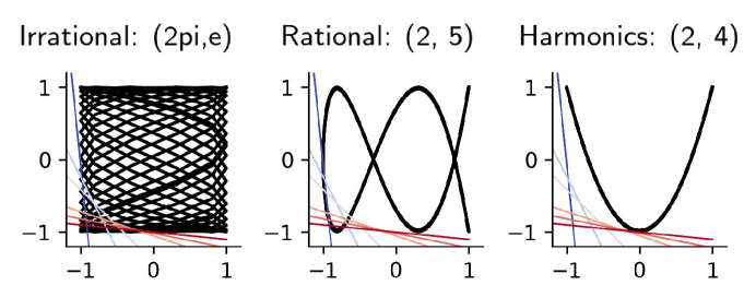
Figure 14: Schematics showing irrational and rational ratio case the data are range dependent beyond the modular-mixed boundary while in de-modularising harmonics case, the two periodic waves are range independent.

Irrational Frequencies Modularise

If $\omega$ is irrational then, by Kronecker’s theorem, you can find a value of $t$ for which $\cos(t)$ and $\cos(\omega t+\phi)$ take any pair of values. This makes the two frequencies, among other things, extreme point independent, and therefore no mixing is better than modularising.

Even Integer Multiples Mix

According to Theorem 2.1, to modularise, for all $\delta$ and $\phi$ values:

$$\Delta>\sqrt{1+\delta^{2}}=1+\mathscr{O}(\delta^{2})$$ (119)

We will therefore try to find a $\delta$ and $\phi$ which breaks this inequality. Consider $\delta<0$ and very small and $\phi=0$, then, writing $\omega=2m$ for integer $m$:

$$\Delta=-\min_{i}[\cos(t)+\delta\cos(2mt)]$$ (120)

$\cos(t)-|\delta|\cos(2mt)$ takes its extreme values when $t$ is an integer multiple of $\pi$, and the smallest it can be is $-1+|\delta|$. Hence:

$$\Delta=1-\delta<1+\mathscr{O}(\delta^{2})$$ (121)

This is smaller than the critical value, so the representation should mix, since at least one mixing inequality was broken.

Odd Integer Multiples Mix

If $\omega$ is an odd integer then we can instead mix cosine with sine by choosing $\phi=\frac{\pi}{2}$:

$$g_{i}(t)=\cos(t)+\delta\sin(\omega t)+\Delta$$ (122)

Then the same argument goes through as above.

Other Rational Multiples Modularise

Now consider $\omega=\frac{p}{q}$ for two integers $p$ and $q\neq 1$. We were inspired in this section by the mathoverflow post of Soudry and Speiser [59]. So we are considering the mixed encoding:

$$g(t)=\cos(t)+\delta\cos(\frac{p}{q}t+\phi)+\Delta$$ (123)

And we have to show that for all $\delta$ and $\phi$, $\Delta^{2}>1+\delta^{2}$. For general $\phi$ we have been unable to do this, but for $\phi=0$ we present proof below in the hope this can be generalised.

We break down the problem into four cases based on the sign of $\delta$, and whether $p$ and $q$ are both odd, or only one is. The easiest is if both are odd, and $\delta>0$. Then take $t=q\pi$:

$$g(t)=\cos(q\pi)+\delta\cos(p\pi)+\Delta=-1-\delta+\Delta>0$$ (124)

Therefore $\Delta$ is at least $1+\delta$, which is larger than $\sqrt{1+\delta^{2}}$, hence modularising is better.

Conversely, if one of $p$ or $q$ is even (let’s say $p$ w.l.o.g.) and $\delta<0$ then choose $t=p\pi$ again:

$$g(t)=-1+\delta\cos(p\pi)+\Delta=-1-|\delta|+\Delta>0$$ (125)

And the same argument holds.

Now consider the case where $\delta>0$ and one of $p$ or $q$ is odd. Then there exists an odd integer $k$ such that[59]:

$$kp=q+1\mod 2q$$ (126)

Therefore take $t=k\pi$:

$$g(t)=\cos(k\pi)+\delta\cos(\pi(\frac{kp}{q}))+\Delta=-1+\delta\cos(\pi(\frac{q+1+2nq}{q}))+\Delta$$ (127)

For some integer $n$. Developing:

$$g(t)=-1-\delta\cos(\frac{\pi}{q})+\Delta$$ (128)

The key question is whether for any $\Delta$ below the critical value this representation is nonnegative. For this to be true:

$$-1-\delta\cos(\frac{\pi}{q})+\sqrt{1+\delta^{2}}\geq 0$$ (129)

Developing this we get a condition on the mixing coefficient $\delta$:

$$\delta\geq\frac{2\cos(\frac{\pi}{q})}{1-\cos^{2}(\frac{\pi}{q})}.$$ (130)

We can apply a similar argument with $t=\frac{qk\pi}{p}$ to get:

$$-\cos(\frac{\pi}{p})-\delta+\Delta\geq 0$$ (131)

This leads us to:

$$\delta\leq\frac{1-\cos^{2}(\frac{\pi}{p})}{2\cos(\frac{\pi}{p})}$$ (132)

We squeeze inequalities eqn.130,132 and get

$$1\leq\frac{(1-\cos^{2}(\pi/p))(1-\cos^{2}(\pi/q))}{4\cos(\pi/p)\cos(\pi/q)}$$ (133)

For any even, odd integer pair of $p,q\neq 1$ and $\delta>0$, $\cos(\pi/p)$ and $\cos(\pi/q)$ are bounded in $(0,1]$. In this case, the maximum possible value of the righthand side is achieved with the smallest possible pair of integers $(3,4)$, for which the inequality does not hold. Thus the inequalities eqn.132, 130 cannot hold at the same time which let us to conclude that there is no $\Delta$ below the critical value satisfying nonnegativity constraint and leads to modular representation.

The last case is where $\delta<0$ and both $p,q$ are odd. We can extend the relation shown in eqn.126 as following by simple substitution of oddity of the variables. With given odd integers $p,q$, there exists an even integer $k$ satisfying eqn.126. Similar to above, take $t=\frac{qk\pi}{p}$ for the mixed encoding eqn.123 and we develop:

$$g_{i}=-\cos(\frac{\pi}{p})+\delta+\Delta$$ (134)

, which leads to the following inequality:

$$\delta\geq\frac{1-\cos^{2}(\pi/p)}{-2\cos(\pi/p)}$$ (135)

Now take $t=k\pi$, and we get:

$$g_{i}=1-\delta\cos(\pi/q)+\Delta$$ (136)

which leads to the in equality,

$$\delta\leq\frac{-2\cos(\pi/q)}{1-\cos^{2}(\pi/q)}$$ (137)

Again, the above two inequalities cannot hold together with the odd integers $p,q>1$.

We also empirically show on Fig 14 that in rational multiple frequencies, there is no modular-mixed boundary possible to break the modularisation.

Appendix D Metrics for Representational Modularity and Source Statistical Interdependence

We seek to design a metric to measure how much information a latent contains about a source. However, we would like to ignore information that could be explained through the latent’s tuning to a different source. For example, perhaps two variables are correlated, if a latent encodes one of them, then it will also be slightly informative about the other despite not being functionally related. We therefore seek to condition on all of the sources bar one, and measure how much information the latent contains about the remaining source.

Dunion et al. [18] leverage conditional mutual information in a similar way to this in a reinforcement learning context, but for training rather than evaluation, and therefore resort to a naive Monte Carlo estimation scheme that scales poorly. Instead, we leverage the identity

$$I({\bm{z}}_{j};{\bm{s}}_{i}|{\bm{s}}_{-i})=I({\bm{z}}_{j};{\bm{s}})-I({\bm{z}}_{j};{\bm{s}}_{-i}),$$ (138)

where ${\bm{s}}_{-i}$ is a shorthand for $\{{\bm{s}}_{i^{\prime}}\;|\;i^{\prime}\neq i\}$. Since this involves computing mutual information with multiple sources, we restrict ourselves to considering discrete sources and use a continuous-discrete KSG scheme [51] to estimate information with continuous neural activities. We normalise conditional mutual information by $H({\bm{s}}_{i}|{\bm{s}}_{-i})$ to obtain a measure in $[0,1]$. We then arrange the pairwise quantities into a matrix ${\bm{C}}\in\mathbb{R}^{d_{s}\times d_{z}}$ and compute the normalised average “max-over-sum” in a column as a measure of sparsity, following Hsu et al. [27]:

$$\mathrm{CInfoM}({\bm{s}},{\bm{z}}):=\left(\frac{1}{d_{z}}\sum_{j=1}^{d_{z}}\frac{\max_{i}{\bm{C}}_{ij}}{\sum_{i=1}^{d_{s}}{\bm{C}}_{ij}}-\frac{1}{d_{s}}\right)\bigg{/}\left(1-\frac{1}{d_{s}}\right).$$ (139)

CInfoM is appropriate for detecting arbitrary functional relationships between a source and a neuron’s activity. However, in some of our experiments, the sources are provided as supervision for a linear readout of the representation. In such cases, the network cannot use information that is nonlinearly encoded, so the appropriate meausure is the degree of linearly encoded information. Operationalising this we leverage the predictive $\mathscr{V}$-information framework of Xu et al. [72]. We specify the function class $\mathscr{V}$ as linear and calculate

$$I_{\mathscr{V}}({\bm{z}}_{j}\to{\bm{s}}_{i}|{\bm{s}}_{-i}) =I_{\mathscr{V}}({\bm{z}}_{j}\to{\bm{s}})-I_{\mathscr{V}}({\bm{z}}_{j}\to{\bm{s}}_{-i})$$ (140)

$$=H_{\mathscr{V}}({\bm{s}})-H_{\mathscr{V}}({\bm{s}}|{\bm{z}}_{j})-H_{\mathscr{V}}({\bm{s}}_{-i})+H_{\mathscr{V}}({\bm{s}}_{-i}|{\bm{z}}_{j}),$$

followed by a normalisation by $H_{\mathscr{V}}({\bm{s}}_{i}|{\bm{s}}_{-i})$. Each predictive conditional $\mathscr{V}$-entropy term is estimated via a standard maximum log-likelihood optimization over $\mathscr{V}$, which for us amounts to either logistic regression or linear regression, depending on the treatment of the source variables as discrete or continuous. The pairwise linear predictive conditional information quantities are reduced to a single linear conditional InfoM quantity by direct analogy to Equation 139.

Finally, to facilitate comparisons across different source distributions, we report CInfoM against the normalised multiinformation of the sources:

$$\mathrm{NI}({\bm{s}})=\frac{\sum_{i=1}^{d_{s}}H(s_{i})-H({\bm{s}})}{\sum_{i=1}^{d_{s}}H(s_{i})-\max_{i}H(s_{i})}.$$ (141)

This allows us to test the following null hypothesis: that breaking statistical independence, rather than range independence, is more predictive of mixing. On the other hand, if range independence is more important, then source distributions that retain range independence while admitting nonzero multiinformation will better induce modularity compared to those that break range independence.

Appendix E What-Where Task

E.1 Experimental Setup

E.1.1 Data Generation

The network modularises when exposed to both simple and complex shapes. Simple shapes, used in all main paper figures, are 9-element one-hots, reflecting the active pixel’s position in a $3\times 3$ grid. Formally, for a shape at position $(i,j)$ in the grid, the corresponding vector $s\in\mathbb{R}^{9}$ is given by:

$$s_{k}=\begin{cases}1&\text{if }k=3(i-1)+j\\ 0&\text{otherwise}\end{cases}$$

where $i,j\in\{1,2,3\}$.

For complex shapes, each shape is a binary vector $c\in\mathbb{R}^{9}$, with exactly 5 elements set to 1 and 4 elements set to 0, representing the active and inactive pixels, respectively. Each complex shape takes the (approximate) shape of a letter (15) and can be shifted to any of the 9 positions in the $3\times 3$ grid. The standard training and testing datasets include one of every shape-position pair. The correlations introduced later include duplicates of a subset of these data points.

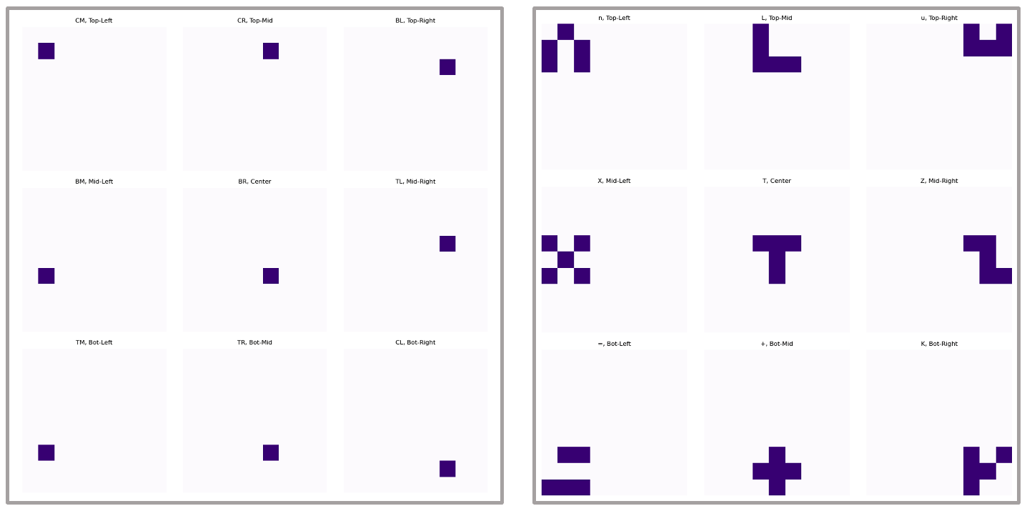
Figure 15: Different possible inputs to the network. Both one-hot (left) and letter-based (right) shapes can be outputted as either a concatenation of one-hots or as a 2D variable.

E.1.2 Network Architecture

The network we use here is designed in PyTorch and takes as input am 81-element vector, flattened to a $9\times 9$ image (15).The network architecture is formally defined as follows:

$$\text{Input:}\quad x\in\mathbb{R}^{81}$$

$$\text{Hidden layer:}\quad\mathbf{h}=\phi(\mathbf{W}_{1}x+\mathbf{b}_{1}),\quad\mathbf{W}_{1}\in\mathbb{R}^{25\times 81},\quad\mathbf{b}_{1}\in\mathbb{R}^{25}$$

$$\text{Output layer:}\quad\mathbf{y}=\mathbf{W}_{2}h+\mathbf{b}_{2},\quad\mathbf{W}_{2}\in\mathbb{R}^{2\times 25},\quad\mathbf{b}_{2}\in\mathbb{R}^{2}$$

where $\phi$ is the activation function, either ReLU or $\tanh$, depending on the experiment. Weights $\mathbf{W}_{1}$ and $\mathbf{W}_{2}$ are initialised with a normal distribution $\mathscr{N}(0,0.01)$, and biases $\mathbf{b}_{1}$ and $\mathbf{b}_{2}$ are initialised to zero.

E.1.3 Training Protocols

The network uses the Adam optimiser ([34]), with learning rate and other hyperparameters varying from experiment to experiment. The mean squared error (MSE) is calculated separately for ‘what’ and ‘where’ tasks, and then combined along with the regularisation terms. The total loss function $L_{total}$ is a combination of the task-specific losses and regularisation terms:

$$L_{total}=L_{what}+L_{where}+\lambda_{R}(||\mathbf{W}_{1}||^{2}_{2}+||\mathbf{W}_{2}||^{2}_{2}+||\mathbf{h}||^{2}_{2})$$

where $L_{task}$ for ‘what’ and ‘where’ tasks is defined as:

$$L_{task}(y,\hat{y})=\frac{1}{N}\sum^{N}_{i=1}(y_{i}-\hat{y_{i}})^{2}$$

Where $\lambda_{R}$ is the regularisation hyperparameter, typically set to $0.01$ unless specified otherwise. The network is trained using the Adam optimiser with a learning rate ranging between $0.001$ and $0.01$, adjusted as needed. Experiments are run for order $10^{4}$ epochs on 5 random seeds. Each experiment was executed using a single consumer PC with 8GB of RAM and across all settings, the networks achieve negligible loss.

E.2 Modularity of What & Where

E.2.1 Biological Constraints are necessary for Modularity

To understand the effect of biological constraints on modularisation, consider the optimisation problem under positivity and energy efficiency constraints. The activation function $\phi(x)$ ensures non-negativity:

$$\phi(x)=\max(0,x)$$

The energy efficiency is enforced by adding an L2 regularisation term to the loss function. By minimising the combined loss function $L_{total}$, the network encourages sparse and low-energy activations, leading to a separation of neurons responding to different tasks (‘what’ and ‘where’).

To illustrate the necessity of biological constraints in the modularisation of these networks, we show below the weights and activity responses of networks for networks where these constraints aren’t present. As discussed above, positivity is introduced via the ReLU activation function, and energy efficiency is defined as an L2 regularisation on the hidden weights and activities.

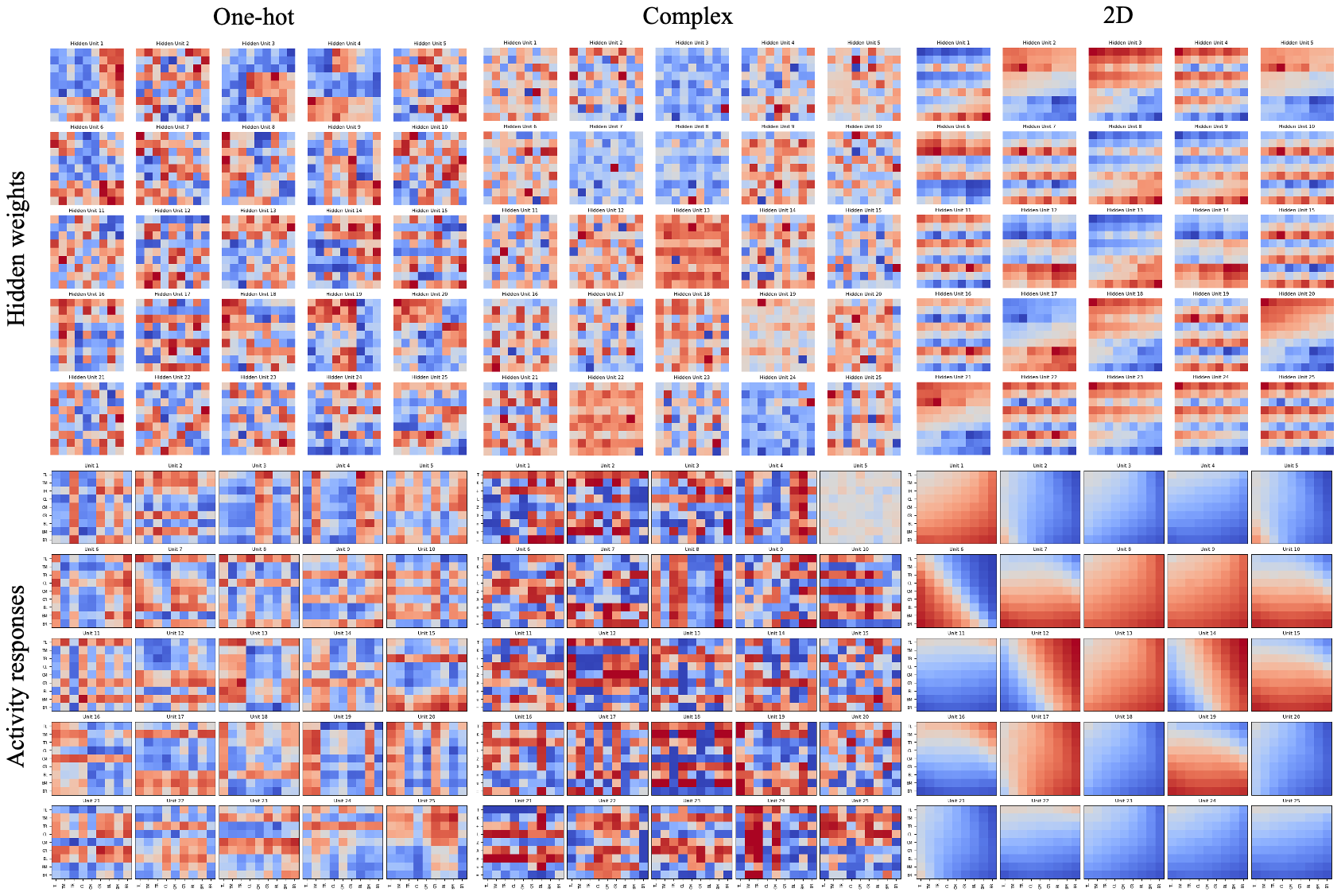
Figure 16: Hidden weights and activity responses of FF networks without biologically-inspired constraints. The one-hot and letter-like binary cases are shown, as well the 2D output setting with one-hot inputs.

As shown in the neural tuning curves, the unconstrained networks do encode task features, but they do so such that each neuron responds to the specific values of both input features, they are mixed selective. Compare these results to the weights and activity responses when positivity and energy efficiency constraints are introduced. In this setting, there is a clear separation of ‘what’ and ‘where’ tasks, into two distinct sub-populations of neurons.

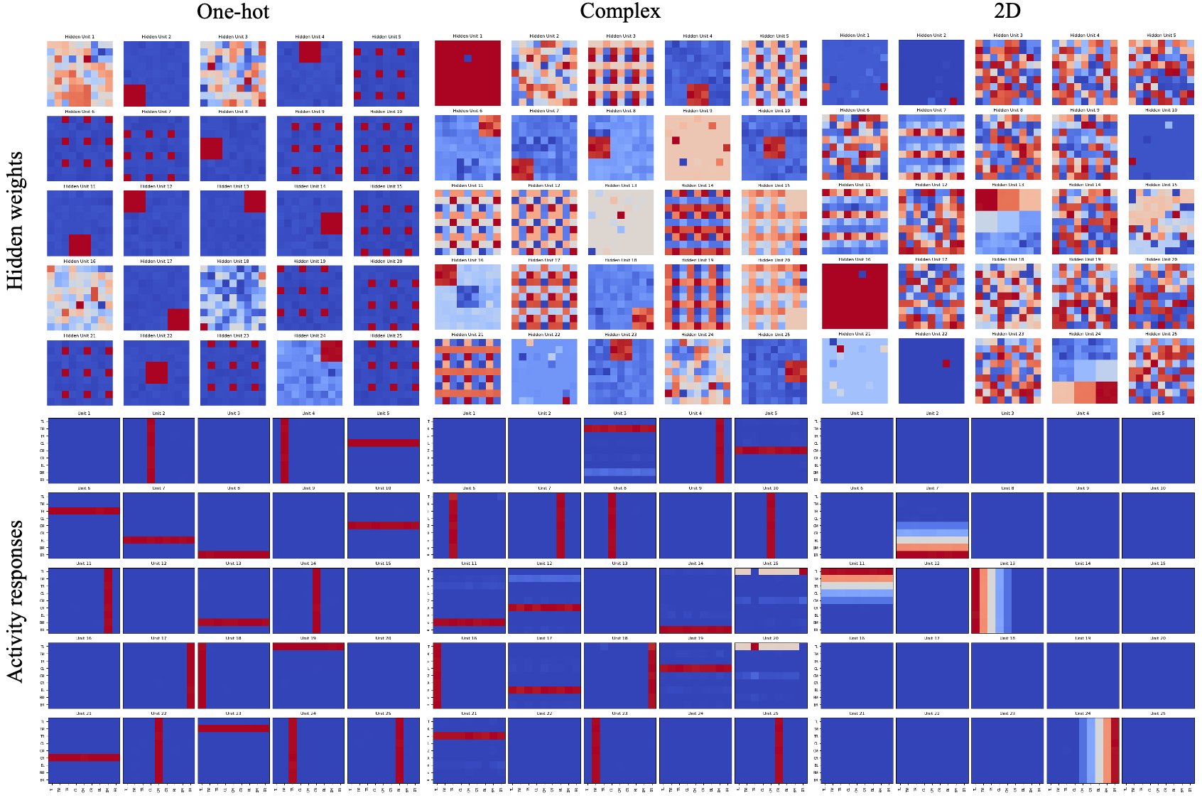
Figure 17: Weights and activity response of networks under biological constraints. The one-hot and letter-like binary cases are shown, as well the 2D output setting with one-hot inputs.

E.3 Dropout & Correlation

We use two different approaches to dropout in order to illustrate the importance of range independence.

Diagonal Dropout: The first approach removes example data points (i.e., shape-position pairs) from elements along the diagonals, starting in the middle and extending out to all four corners. This has the effect of increasing the mutual information between data sources but does not significantly affect their range dependence. Formally, let $D$ be the set of all shape-position pairs. In the diagonal dropout setting, we remove pairs $(s_{i},p_{i})$ where $i$ lies along the diagonal of the input grid:

$$D^{\prime}=D\setminus\{(s_{i},p_{i})\mid i\in\text{diagonal positions}\}$$

In the most extreme case, only one data point from each corner is removed, and this is not sufficient to force mixed-selectivity in the neurons.

Corner Dropout: The second approach removes data points from one corner of the distribution. This also increases the mutual information between sources but changes their extreme-point dependence. Specifically, we remove pairs $(s_{i},p_{i})$ where $i$ lies in the bottom-left corner of the input grid:

$$D^{\prime\prime}=D\setminus\{(s_{i},p_{i})\mid i\in\text{bottom-left corner positions}\}$$

In this setting, a single data point removed from the corner is insufficient for breaking modularity; however, removing more than this causes mixed selective neurons to appear.

Correlation: To correlate sources, we duplicate data points that appear along the diagonal. This increases the mutual information between sources without affecting their range independence:

$$D^{\prime\prime\prime}=D\cup\{(s_{i},p_{i})\mid i\in\text{diagonal positions}\}$$

The mutual information $I(X;Y)$ between the shape $X$ and position $Y$ is calculated as follows:

$$I(X;Y)=\sum_{x,y}P(x,y)\log\frac{P(x,y)}{P(x)P(y)}$$

where $P(x,y)$ is the joint probability distribution of $X$ and $Y$.

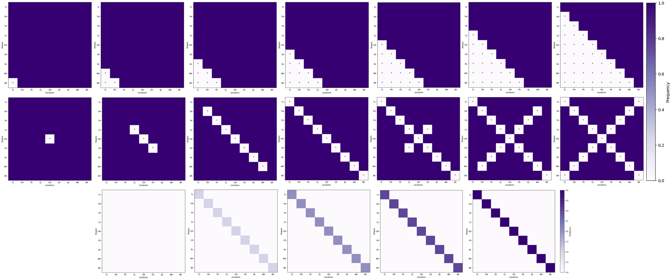
Figure 18: Increasing dropout (left to right) for both the corner-cutting (top) and diagonal (middle) cases, as well as correlation distributions (bottom). Note: asterisk denotes the absence of training data for this pair of input features.

Appendix F Nonlinear Autoencoders

F.1 Autoencoding Sources

Three-dimensional source data is sampled from $[0,1]^{3}$ and discretised to 21 values per dimension. The encoder and decoder are each a two-layer MLP with hidden size 16 and ReLU activation. The latent bottleneck has dimensionality six. All models use $\lambda_{\text{reconstruct}}=1$, $\lambda_{\text{activity energy}}=0.01$, $\lambda_{\text{activity nonnegativity}}=1$, and $\lambda_{\text{weight energy}}=0.0001$. Models are initialised from a He initialisation scaled by 0.3 and optimized with Adam using learning rate 0.001. Each experiment was executed using a single consumer GPU on a HPC with 2 CPUs and 4GB of RAM.

F.2 Autoencoding Images

We subsample 6 out of the 9 sources in the Isaac3D dataset, fixing a single value for the other 3. This yields a dataset of size $12,288$. We use an expressive convolutional encoder and decoder taken from the generative modeling literature. We use 12 latents, each quantised to take on 10 possible values. We use a weight decay of 0.1 and a learning rate of 0.0002 with the AdamW optimizer. Each experiment was executed using a single consumer GPU on a HPC with 8 CPUs and 8GB of RAM.

Appendix G Recurrent Neural Networks

G.1 Linear and Nonlinear Periodic Wave RNN Experiment Details

For linear RNN, we considered a task where the RNN gets a periodic pulse input (2D delta function of frequencies $w_{1},w_{2}$ as input $x$, i.e. $x_{k}(t)=\delta(\cos(w_{k}t)-1),k\in\{1,2\}$) and learns to generate a 2D cosine wave of the same frequencies, $y_{k}(t)=\cos(w_{k}t)$.

For the nonlinear RNN, we designed a two frequency mixing task. Given two source frequencies, the network must generate two cosine waves whose frequencies are the sum and difference of two input frequencies. The network requires non-linearities in order to approximate the multiplication: $\cos(a+b)=\cos(a)\cos(b)-\sin(a)\sin(b),\cos(a-b)=\cos(a)\cos(b)+\sin(a)\sin(b)$. In the task, the RNN receives 2D periodic delta pulse of frequency $\frac{w1+w2}{2}$ and $\frac{w1-w2}{2}$ and learns to generate a trajectory of $\cos(w_{1})$ and $\cos(w_{2})$.

We use the following recurrent neural network,

$$\mathbf{g}(t+1)=f(\mathbf{W_{\text{rec}}}\mathbf{g}(t)+\mathbf{W_{\text{in}}}+\mathbf{b_{\text{rec}}})$$ (142)

$$\mathbf{y}(t)=\mathbf{R}\mathbf{g}(t)+\mathbf{b_{\text{out}}}$$ (143)

in our linear RNNs $f(\cdot)$ is identity whereas in the nonlinear ones we used $ReLU$ activation to enforce positivity condition.

For irrational output frequency ratio case, we used

$$w_{1}=p\pi,w_{2}=\sqrt{q},p\sim\mathscr{U}(0.5,4),q~{}\sim\mathscr{U}(1,10).$$ (144)

For rational case, we sampled

$$w_{1},w_{2}\in[1,20]\cap\mathbb{Z}.$$ (145)

Where $\mathbb{Z}$ is the set of integers. For harmonics:

$$w_{1}\in[1,10]\cap\mathbb{Z},w_{2}=2w_{1}.$$ (146)

We trained RNN with the trajectory of length $T=200$, bin size $0.1$, and hidden dimension 16. For the linear RNN, we used learning rate 1e-3, 30k training iterations and $\lambda_{\text{target}}=1$, $\lambda_{\text{activity}}=0.5,\lambda_{\text{positivity}}=5,$ and $\lambda_{\text{weight}}=0.02$. For the nonlinear RNN, we used learning rate 7.5e-4, 40k training iterations and $\lambda_{\text{target}}=5,\lambda_{\text{activity}}=0.5$ and $\lambda_{\text{weight}}=0.01$. In both case, we initialised the weights to be orthogonal and the biases at zero, and used Adam optimiser.

To assess the modularity of the trained RNNs, we performed a Fast Fourier Transform(FFT) on each neuron’s activity and measured the relative power of the key frequencies $w1,w2$ with respect to the sum of total power spectrum

$$C_{\text{neuron}_{i},w_{j}}=\frac{|FFT(g_{i};w_{j})|}{\sum_{f}{|FFT(g_{i};f)|}}$$ (147)

and used it as a proxy of mutual information for modularity metric introduced in eqn. 139.

G.2 Nonlinear Teacher-Student RNNs

Network details. The Teacher network has input, hidden, and output dimensions of 2, and has orthogonal recurrent weights, input weights, and output weights. The Student RNN has input dimension 2, output dimension 2, and hidden dimension 64. It is initialised as per PyTorch default settings. The Teacher network dynamics is a vanilla RNN: ${\bm{h}}_{t}=tanh({\bm{W}}_{rec}{\bm{h}}_{t-1}+{\bm{W}}_{in}{\bm{i}}_{t})$, and each teacher predicts a target via ${\bm{o}}_{t}={\bm{W}}_{out}{\bm{h}}_{t}$. The Student RNN has identical dynamics (but with a ReLU activation function, and different weight matrices etc).

Generating training data. The teacher RNN generates training data for the Student RNN. We want to tightly control the Teacher RNN hidden distribution (for corner cutting or correlation analyses), i.e., tightly control the source distribution for the training data. To control the distribution of hidden activities of the Teacher RNN, we use the following procedure. 1) We sample a randomly initialised Teacher RNN. 2) ${\bm{h}}_{0}$ is initialised as a vector of zeros. 3) With a batch size of $N$, we take a single step of the Teacher RNN (starting from 0 hidden state) assuming ${\bm{i}}_{t}=0$. This produces network activations (for each batch), ${\bm{p}}_{t}=tanh({\bm{W}}_{rec}{\bm{h}}_{t-1}$. 4) We then sample from idealised distribution of the teacher hidden states, ${\bm{h}}_{t}$. For example a uniform distribution, or a cornet cut distribution. At this point these are just i.i.d. random variables, and not recurrently connected. 5) To recurrently connect these points, we optimise the input to the RNN, ${\bm{i}}_{t}$, such that the RNN prediction, ${\bm{p}}_{t}$, becomes, ${\bm{h}}_{t}$. We then repeat steps 3-5) for all subsequent time-steps, i.e., we find what the appropriate inputs are to produce hidden states as if they were sampled from an idealised distribution. To prevent the Teacher RNN from being input driven, on step 4), we solve a linear sum assignment problem across all batches ($N$ batches), so the RNN (on average) gets connected to a sample ,${\bm{h}}_{t}$, that is close to its initial prediction, ${\bm{p}}_{t}$. This means the input, ${\bm{i}}_{t}$, will be as small as possible and thus the Teacher RNN dynamics are as unconstrained as possible.

Training. We train the Student RNN on $10000$ sequences generated by the Teacher RNN. The learning objective is a prediction loss $|{\bm{o}}^{teacher}_{t}-{\bm{o}}^{student}_{t}|^{2}$ plus regularisation of the squared activity of each neuron as well as each synapse (both regularisation values of 0.1). We train for 60000 gradient updates, with a batch size of 128. We use the Adam optimiser with learning rate 0.002.

Appendix H Neural Data Analysis

We were kindly given the data of Xie et al. We used it to generate Figure 4B. In this section we talk through our analysis techniques. First, however we discuss methods for measuring subspace alignment.

H.1 Subspace Alignment Metrics

Previous works have calculated a single angle between subspaces, most rigorously the first principal angle [71], alternatively the unique angle between the two subspaces after projecting to a three dimensional PC space. We found that these angle based methods were biased for two reasons.

First, two $N$ dimensional subspaces have $N$ principal angles, and these are ordered, the first principal angle is smaller than the second, which is smaller than the third, etc. This ordering means that noise added to a representation will bias the estimates of the first principal angles down, and the last ones up. To show this we created data that lives in two planes oriented at 72 degrees. We then add guassian noise and find that this biases the estimate of the first principal angle down, and the second up, despite the fact that they are both 72, Figure 19.

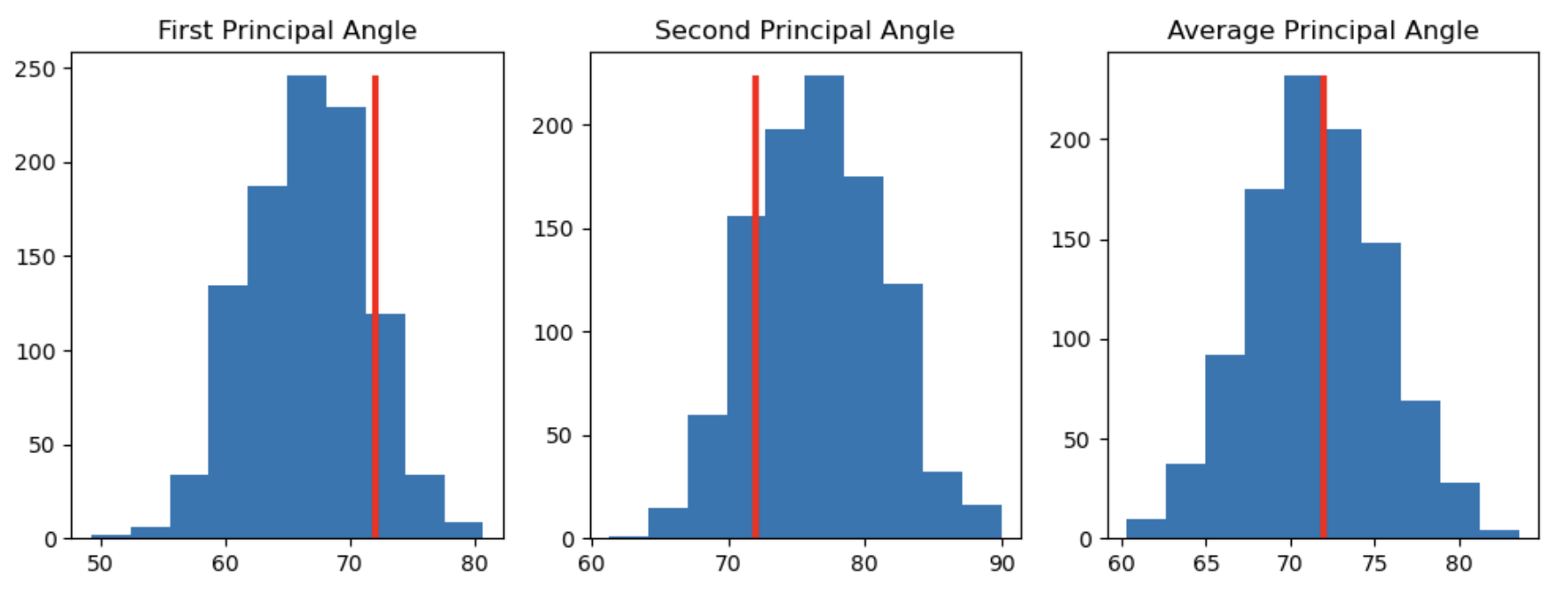
Figure 19: We create some fake data of two 2D subspaces that are aligned at $72^{\circ}$, i.e. both of the two principal angles are $72^{\circ}$. We then add a small amount of noise 1000 times and calculate the principal angles between the noisy vectors (all the vectors are length one, and I add a zero-mean gaussian noise matrix with variance 0.1). As you can see, the estimate of the first principal angle is biased down, the second up, but the average appears unbiased.

Second, without further thought, angles are bounded, since they are necessarily smaller than 90. If your true data is oriented close to 90 degrees that means that noise will more likely push your estimate away from 90 than towards it. To show this effect we create another noisy dataset at 85 degrees, and show the noise pushes all estimates, even the mean of the two angles, significantly below 85, Figure 20.

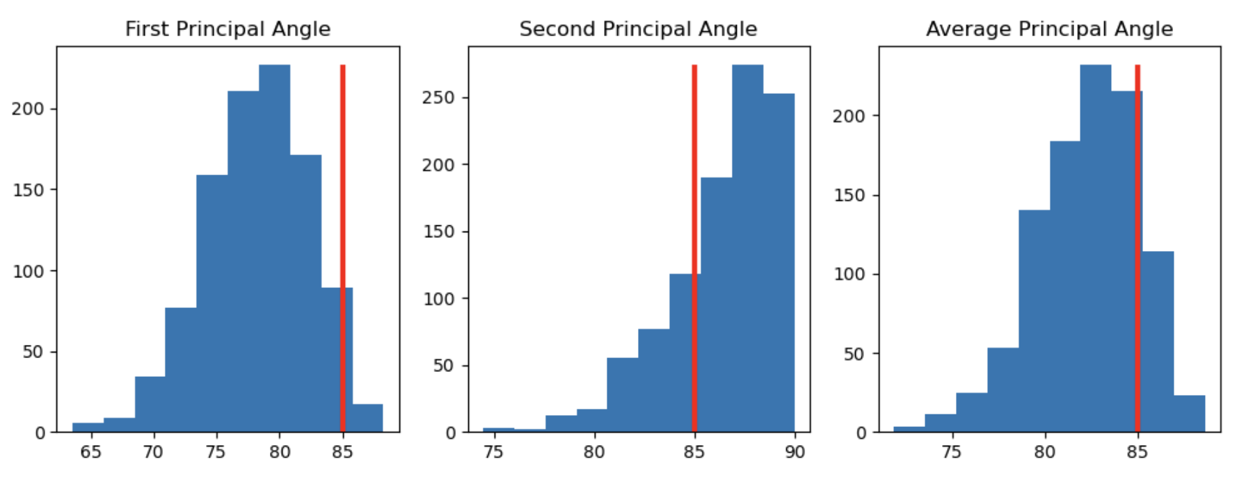
Figure 20: Same setting as figure 19, except now the true principal angle is $85^{\circ}$. We can see that all estimators of the average principal angle are shifted downwards.

We counteract both these effects by using a single metric, whose bounds are nowhere near the ranges of interest. Specifically we use the correlation metric from Panichello & Buschmann. Given a set of vectors from the two subspaces of interest: $\{{\bm{g}}(c,s)\}_{c=1,s=1}^{C,2}$, indexed by subspace $s$ and condition $c$ (for example, which cue was presented), the correlation is:

$$\rho=\langle\text{corr}({\bm{g}}(c,1)-\langle{\bm{g}}(c^{\prime},1)\rangle_{c^{\prime}},{\bm{g}}(c,2)-\langle{\bm{g}}(c^{\prime},2)\rangle_{c^{\prime}}\rangle_{c}$$ (148)

Where the correlation is over neurons. This is 0 when subspaces are orthogonal, and avoids both pitfalls. Panichello & Buschman reported this metric on their data. We therefore move to extract the same metric from the data of Xie.

H.2 Extracting Coding Subspaces from Sampled without Replcement Sequences

We analyse the firing rates that came pre-extracted from calcium imaging by Xie et al. We study the delay period representation of the two-sequence task. Call the neural representation of a two element sequence during the delay period ${\bm{g}}(\begin{bmatrix}\theta_{1}\\ \theta_{2}\end{bmatrix})$. We make the assumption (supported by data [19, 71, 45] and simulations [8, 70]) that the data decomposes into subspaces encoding each sequence element: ${\bm{g}}(\begin{bmatrix}\theta_{1}\\ \theta_{2}\end{bmatrix})={\bm{g}}_{1}(\theta_{1})+{\bm{g}}_{2}(\theta_{2})+{\bm{c}}$, where ${\bm{g}}_{i}(\theta)$ denotes the activity in subspace $i$ when the $i$’th element of the sequence is $\theta$. If the sequences are sampled with replacement the two sequence elements are uncorrelated and you can find ${\bm{g}}_{1}(\theta_{1})$ up to a constant offset by just averaging over the other sequence element, ${\bm{g}}_{1}(\theta_{1})=\langle{\bm{g}}(\begin{bmatrix}\theta_{1}\\ \theta_{2}\end{bmatrix})\rangle_{\theta_{2}}={\bm{g}}_{1}(\theta_{1})+\langle{\bm{g}}_{2}(\theta)\rangle_{\theta}+{\bm{c}}$, where $\langle\rangle$ denotes averaging. Performing PCA on the set of $\{{\bm{g}}_{1}(\theta_{i})\}_{i=1}^{Q}$ then gets you a perfect estimate of the subspace containing information about $\theta_{1}$, as it removes the shared constant offset. This process does not work if the sequences are sampled without replacement, as you cannot perform the $\langle{\bm{g}}_{2}(\theta)\rangle_{\theta}$ average.

Xie et al. get around this problem by doing regularised linear regression. To remove any potential hyperparameter dependence we employ a novel difference scheme. Consider the following term:

$$\Big{\langle}{\bm{g}}\Big{(}\begin{bmatrix}\theta_{1}\\ \theta_{2}\end{bmatrix}\Big{)}-{\bm{g}}\Big{(}\begin{bmatrix}\theta^{\prime}_{1}\\ \theta_{2}\end{bmatrix}\Big{)}\Big{\rangle}_{\theta_{2}}$$ (149)

Equal to:

$$\frac{Q-2}{Q}\Big{\langle}{\bm{g}}\Big{(}\begin{bmatrix}\theta_{1}\\ \theta_{2}\end{bmatrix}\Big{)}-{\bm{g}}\Big{(}\begin{bmatrix}\theta^{\prime}_{1}\\ \theta_{2}\end{bmatrix}\Big{)}\Big{\rangle}_{\theta_{2}\neq\theta_{1},\theta^{\prime}_{1}}+\frac{1}{Q}\Big{(}\underbrace{{\bm{g}}\Big{(}\begin{bmatrix}\theta_{1}\\ \theta_{1}\end{bmatrix}\Big{)}-{\bm{g}}\Big{(}\begin{bmatrix}\theta^{\prime}_{1}\\ \theta_{1}\end{bmatrix}\Big{)}+{\bm{g}}\Big{(}\begin{bmatrix}\theta_{1}\\ \theta^{\prime}_{1}\end{bmatrix}\Big{)}-{\bm{g}}\Big{(}\begin{bmatrix}\theta^{\prime}_{1}\\ \theta^{\prime}_{1}\end{bmatrix}\Big{)}}_{\text{Error Term}}\Big{)}$$ (150)

Again, the left hand side is what we want, the first term on the right is something we can get, and the leftover part is going to be ignored, our error term. Why have we chosen to leave this particular term out? Using the decomposition property of our representations we can see that the thing we want to estimate is:

$$\Big{\langle}{\bm{g}}\Big{(}\begin{bmatrix}\theta_{1}\\ \theta_{2}\end{bmatrix}\Big{)}-{\bm{g}}\Big{(}\begin{bmatrix}\theta^{\prime}_{1}\\ \theta_{2}\end{bmatrix}\Big{)}\Big{\rangle}_{\theta_{2}}={\bm{g}}_{1}(\theta_{1})-{\bm{g}}_{1}(\theta^{\prime}_{1})$$ (151)

Which makes sense, it is the difference in subspace 1 between the encoding of these two stimuli. But now we can analyse the error term and see that it is equal to the same thing!

$${\bm{g}}\Big{(}\begin{bmatrix}\theta_{1}\\ \theta_{1}\end{bmatrix}\Big{)}-{\bm{g}}\Big{(}\begin{bmatrix}\theta^{\prime}_{1}\\ \theta_{1}\end{bmatrix}\Big{)}+{\bm{g}}\Big{(}\begin{bmatrix}\theta_{1}\\ \theta^{\prime}_{1}\end{bmatrix}\Big{)}-{\bm{g}}\Big{(}\begin{bmatrix}\theta^{\prime}_{1}\\ \theta^{\prime}_{1}\end{bmatrix}\Big{)}=2({\bm{g}}_{1}(\theta_{1})-{\bm{g}}_{1}(\theta^{\prime}_{1}))$$ (152)

Hence, plugging these into equation 149:

$$\Big{\langle}{\bm{g}}\Big{(}\begin{bmatrix}\theta_{1}\\ \theta_{2}\end{bmatrix}\Big{)}-{\bm{g}}\Big{(}\begin{bmatrix}\theta^{\prime}_{1}\\ \theta_{2}\end{bmatrix}\Big{)}\Big{\rangle}_{\theta_{2}\neq\theta_{1},\theta^{\prime}_{1}}={\bm{g}}_{1}(\theta_{1})-{\bm{g}}_{1}(\theta^{\prime}_{1})$$ (153)

So we can see that this object is a good estimator of this quantity!

This is therefore the quantity we estimate. For all different stimuli pairs $\theta,\theta^{\prime}$, we build an estimate of the difference vectors. We then use these vectors to calculate the correlation alignment measure 148, this result is reported in Figure 4B. We form error bars by subsampling by half the number of neurons 200 times and estimating the mean and variance over 200 simulations.

H.3 Extracting Encodings from Single-Element ‘Sequenece’ Data

Finally, we need to choose how to encode the memories in the Xie task for our RNN models to use, see Appendix I. We take a data driven approach and estimate the monkey’s internal representation of each cue by analysing the trials in which the only a single stimulus was presented. We average these trials to create six encoding vectors, then find the dot product similarity matrix of this data. Finally, we find a set of 5 dimensional encodings that exactly recreate this data dot product structure. These are the vectors we feed our RNN: they have the same similarity structure as the monkey’s representation, without increasing training time by introducing a neuron-dimensional weight matrix.

Appendix I RNN Models of Neuroscience Tasks

We now talk through the biologically inspired linear RNNs used in sections 5 onwards of the main paper.

I.1 Xie Task, Model, and Extended Results

Each RNN is trained on many sequences. For each sequence the RNN sees two cue encodings, sampled from a set of six $\{{\bm{e}}_{i}\}_{i=1}^{6}$. During the first two timesteps the model is shown the two cues, then recieves no further input. Then there is a delay timestep. Finally in the last two timesteps the model must use an affine output to recreate the two encodings. The recurrent dynamics are simple linear systems:

$${\bm{g}}_{t+1}={\bm{W}}_{\text{rec}}{\bm{g}}_{t}+{\bm{W}}_{\text{in}}{\bm{e}}_{t,i_{t}}+{\bm{b}}\qquad{\bm{e}}_{t,i_{t-3}}={\bm{W}}_{\text{out}}{\bm{g}}_{t}+{\bm{b}}_{\text{out}}$$ (154)

${\bm{g}}_{0}=0$. We train the networks using gradient descent to perfectly solve the task while ensuring the representation is positive. Further, we penalise the L2 norm of the activity and the weights. We used a single set of hyperparameters to generate all data that can be found in the supplementary code.

We played with three different memory encoding schemes, either a 6 dimensional one-hot code, 6 two-dimensional points drawn evenly from the unit circle (like the positions of the dots on the screen shown to the monkey), or the data driven encoding discussed in the Appendix H. Finally, we used two different sequence structures: sampling both sequence elements uniformly, or sampling them without replacement but otherwise uniformly, as in the experiments.

We analysed the resulting delay period activity using the techniques discussed in Appendix H. We found, first, that in all cases, the delay period activity for networks trained on sequences sampled with replacement comprised two orthogonal subspaces. Second, depending on the encoding scheme, some networks trained on sequences sampled without replacement were orthogonal, others aligned, and the degree of alignment depending on the hyperparameter weighting of the activity vs. weight loss. Third, in both sequence settings we also found that the subspace encoding the first memory was a small amount bigger than the second, matching data. We now talk through some of these results in more detail.

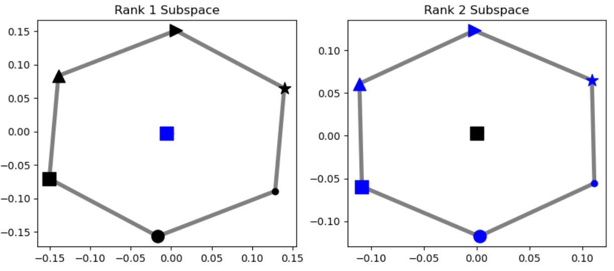
Figure 21: We estimate the two-dimensional subspaces encoding, the two subspaces are basically orthogonal, the circular mean of the 2 principal angles between the subspaces is $89.95^{\circ}$

First, of the three encoding schemes we find that the 2D data is orthogonalised when sampled without replacement (Fig 21), while the one-hot (not shown) and data driven codes do not (Figure 4B). It was this puzzling discrepancy between the behaviour of the one-hot and 2D codes that led us to the data-driven encoding. This behaviour can be somewhat understood by looking at the joint distribution of the encoded memories, figure 22. The required inequality constraint is not satisfied, while it is for 1-hot memories. The neural data inspired encoding presumably lies closer to the 1-hot end of the spectrum.

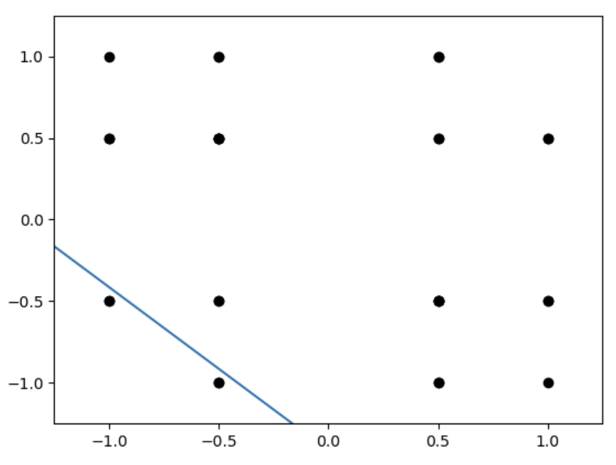
Figure 22: Left: We plot the joint distribution of one dimension of each of the memories against one another for the 2D coding. The x axis is cosine of the first sequence element, the y axis is the second. Sampling without replacement removes the two extreme corner points (but not the whole diagonal, as though this dimension of the code might be equal, the memory is 2D, and the other dimension can be different). The line marks one of the inequality constraints that can be broken to induce mixing. As can be seen, removing one data point is not sufficient to remove all data below this line, so the code modularises. Right: The converse is true for one-hot variables.

We return to the alignment of correlated sequences after discussing the similar results from the Panichello & Buschmann studies.

I.2 Panichello & Buschmann, Model, and Extended Results

We study a very similar linear RNN setting, the loss, training protocol, and sequence structures are mostly identical to the previous section. We list the differences. First, we assume the memory encoding is the equivalent of the 2D one from the previous section.

Second, network architecture: rather than providing inputs to the linear network, we let the network learn the input by allowing it to initialise itself differently depending on the pair of stimuli. This was an implementational choice that doesn’t constrain the input to be a linear function of the encodings. Nonetheless, the network learns to initialise itself as a linear function of the two presented cues. We could equally have provided the two cues as inputs as in the previous section, it would likely have changed little.

Third, we implement the different cues by updating the initial representation with different matrices. If the animal is cued to attend to the top stimulus the initial activity, which we think of as the delay period activity, ${\bm{g}}_{0}(c_{\text{top}},c_{\text{bottom}})$ for two colours $c_{\text{top}}$ and $c_{\text{bottom}}$, is updated using one matrix, which then drives the readout:

$${\bm{W}}_{\text{top}}{\bm{g}}_{0}(c_{\text{top}},c_{\text{bottom}})+{\bm{b}}_{\text{top}}={\bm{g}}_{1}(c_{1},c_{2})\quad{\bm{R}}{\bm{g}}_{1}(c_{\text{top}},c_{\text{bottom}})+{\bm{b}}_{\text{out}}={\bm{e}}_{c_{\text{top}}}$$ (155)

And the same for the bottom matrix. This is inspired by recent work that has shown these type of action dependent matrices are both mathematically tractable, and biologically plausible [40, 14, 68, 70, 69].

Fourth, Number of Samples: in the real experiment Panichello & Buschman present colours drawn from a continuous colour wheel. They then analyse it by binning the colour wheel into groups of four. We skip straight to the binned colours, and pretend the encoded cues that the network predicts are 4 points sampled evenly from the unit circle. Other than this change the sampling schemes are the same.

We extract the subspaces and their alignemnts as discussed in Appendix H. We make some final interesting (to us!) observations. First, the top and bottom colour subspaces are equally sized, unlike in Xie et al., likely because they are equally important, whereas in the Xie task one stimuli has to be recalled before the other, making it, temporally, more important. Second, since we only sample 4 ‘colours’ from the circle, rather than the 6 in Xie et al., the prediction shown in figure 22 changes. With four data points even 2D encodings are missing the appropriate corner 23!

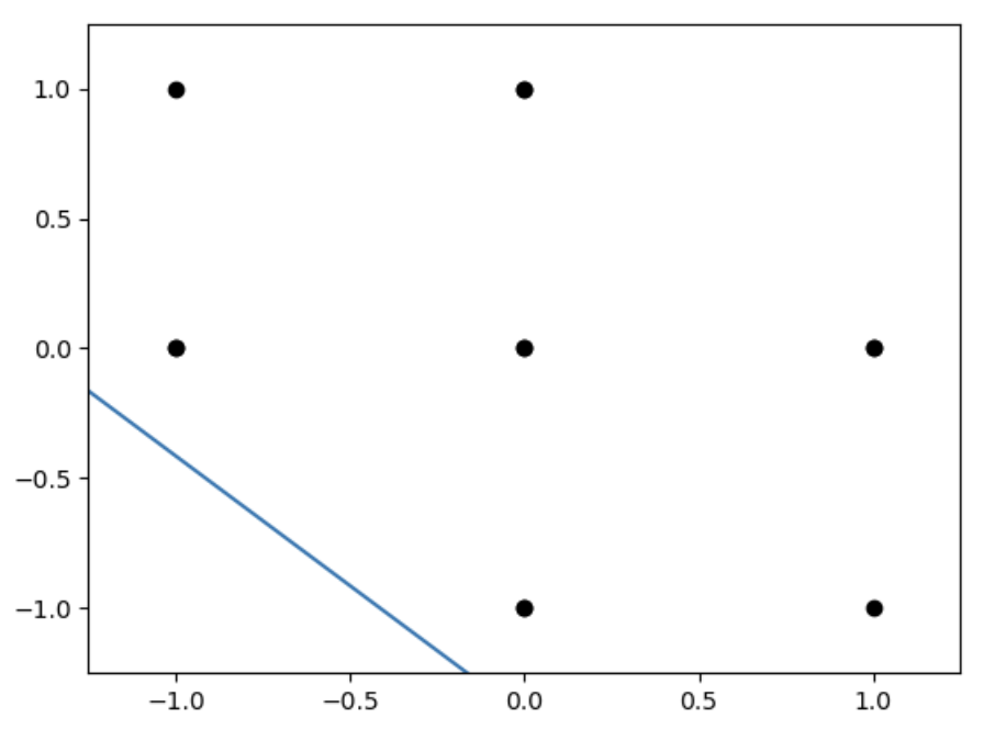
Figure 23: As in 22, we plot the joint distribution of one dimension of each of the memories against one another for the 2D coding. The x axis is cosine of the first sequence element, the y axis is the second. Since there are now only 4 settings of the angle we can see sufficient corner has been removed to predict mixing, as we see in simulations Figure 4.

This matches the finding presented in Figure 4, that when sampled without replacement the subspaces align, since a sufficiently large corner is missing.

Finally, there remain discrepancies between the neural data and our theory and models. Most fundamentally, both theory and models predict that if the subspaces are orthogonal they should be encoded by disjoint groups of neurons, if they align, they should not. Yet, both Xie and Panichello and Buschman find neurons tuned to both cues. This is expected for Xie’s data, but not for Panichello and Buschman’s, where they find roughly 20% of colour tuned neurons are mixed selective. We do not yet have a good understanding of this discrepancy. More superificially, we are not able to fit the exact numerical value of the alignment between subspaces in Xie et al.’s data, and we remain unsure whether this could be done with different hyperparameters or a noise model. We leave this for further exploration in a more targeted venue.

I.3 Motor Subspace Model

To study preparatory and potent subspaces we train ReLU RNNs on simple reach tasks. Each reach is defined as a one-hot code, such as a location to reach towards. The one-hot part of the network’s input tells it which reach it will have to perform next, but not when. A final dimension of the input encodes the go signal saying ’on the next time step do the cued reach!’. The network is then trained to output the cued-one-hot code for a couple of timesteps after the go cue. The network is either trained on a variety of single-reaches, or two reaches cued one after the other.

We then measure how aligned the preparatory and potent subspaces are. Following [21, 75] we gather the activity in the network during single-reach tasks and break it into preparatory - activity after the cue has been presented but before the network outputs anything - and potent - activity during the reach - activity. We then perform PCA on these two sets of activity. We build subspaces made from a subset of these principal components: if the neural activity projected along a principal component captures more than $0.1\%$ of the total variance of that neural activity (preparatory or potent) we include it. We then measure how much of one type of neural activity (preparatory or potent) is captured after projecting to the other subspace.

I.4 Warden & Miller Task, and Model

In the task two images sampled without replacement from a set of four are shown to the animal with delay periods in between. The animal then has to report its memory of the images in a couple of different ways.

We use the same linear RNN as before, but with three differences. First, we include a delay period between the first and second cue, and the second cue and the report time. Second, to take into account the heterogenous nature of the report, we simply ask the network to output 2 4-dimensional one-hot vectors, corresponding to the images presented first and second. Third, we use a different weight update matrix during delay times and cue presentation times. So at times C1 and C2 (Figure 7 H, I) we use one recurrent weight and bias, during the delay period we use another. This was to enable such a simple linear system to solve the task in a minimal way.

To create the plots we perform the same analysis as [41], we average the neural firing rates at each timepoint according to which stimulus was presented first or second. We find many neurons that code for stimulus-time conjunctions, and fewer that code for only time, and they tended to fire around cue times. Note these averages do not take account of the correlations between the two images, introduced by sampling without replacement. As such, the tuning curves cannot be interpreted as evidence of mixed selectivity: in fact these neurons are modular, they respond only to a single stimulus. The other bumps in firing are induced by the task structure. Since the sequences are sampled with replacement our networks have other neurons that are linearly mixed selective to the two cues, as you would expect from our theory.

I.5 Entorhinal Model for Missing Variables Task, and Mixed Spatial-Reward Coding

Our final biological RNN model is inspired by the entorhinal literature and linear network models of it [14, 68, 70, 69]. We used this model to model mixed spatial and reward coding Section 7, and mixed selectivity induced by missing correlated objectsSection 8.

In each trial the agent navigates a 3x3 periodic environment. The RNN receives one special input only at timepoint 0 that tells it the layout of the room. Otherwise at each timestep it is told which action (north, south, east, west), the agent took. It uses this action to linearly update its hidden state:

$${\bm{g}}_{t}={\bm{W}}_{a_{t}}{\bm{g}}_{t-1}+{\bm{b}}_{a_{t}}$$ (156)

At each timestep it has to output, via an affine readout, a particular target depending on the task.

In the spatial-reward task, at timepoint 0 the agent starts at a consistent position and receives an input that is a 9-dimensional 1-hot code telling the agent the relative position of the reward. At each timestep the agent then has to output two 9-dimensional 1-hot codes, one signalling its position in the room, the other the relative displacement of the reward from its position.

The agent experiences many rooms. Across rooms the rewards are either randomly sampled (random rooms), or sampled from one of two fixed positions (fixed rooms). Each agent experiences a different mixture of randomly sampled or fixed rooms. We then optimise the network to perform the task with non-negative neural activities while penalising the L2 norm of the activity and all weight matrices.

In the mixed-selectivity task there are three objects in each room and the agent has to report the relative displacement of each of them. The input at the start of each trial is a 27-dimensional code signalling where the three objects are relative to its own position. As such, as the agent moves around the room it has to keep track of the three objects. This task was harder to train so we moved from the mean squared error to the cross-entropy loss and found it worked well, apart from that all details of loss and training are the same.

Between trials we randomise the position of the objects. Some portion (0.8) of the time these positions are drawn randomly (including objects landing in the same position). The rest of the time the objects were positioned so that the first object was one step north-east of the second, which itself was one step north-east of the third. This introduced correlations between the positions of the objects, while preserving their range independence - all objects could occur in all combinations.

We measured the linear NCMI between the neural activity and the 27-dimensional output code and found that each neuron was informative about a single source, as expected, it had modularised Figure 7C. However, pretend we did not know the third object existed. Perhaps it is a location the mouse cares about, but no experimenter could ever be expected to guess, such as its favourite corner, toilet spot, or scratching post - all good things to keep oriented in your mind. Instead we would calculate the linear NCMI between each neuron and those objects we know to exist. We would still find modular codes for these objects, but we would also find that the neurons that in reality code for third object, due to the correlations between object placements, are actually informative about the first and second object, so they look mixed selective! The position of the objects is always informative about each other, but by conditioning on each object we are able to remove this effect with our metric and uncover the latent modularity. But without knowing which latents to condition on we cannot proceed, and instead get lost in correlations.

References

- Aso et al. [2014] Yoshinori Aso, Daisuke Hattori, Yang Yu, Rebecca M Johnston, Nirmala A Iyer, Teri-TB Ngo, Heather Dionne, LF Abbott, Richard Axel, Hiromu Tanimoto, et al. The neuronal architecture of the mushroom body provides a logic for associative learning. elife, 3:e04577, 2014.
- Attneave [1954] Fred Attneave. Some informational aspects of visual perception. Psychological review, 61(3):183, 1954.
- Barack and Krakauer [2021] David L Barack and John W Krakauer. Two views on the cognitive brain. Nature Reviews Neuroscience, 22(6):359–371, 2021.
- Barlow et al. [1961] Horace B Barlow et al. Possible principles underlying the transformation of sensory messages. Sensory communication, 1(01), 1961.
- Bell and Sejnowski [1995] Anthony J Bell and Terrence J Sejnowski. An information-maximization approach to blind separation and blind deconvolution. Neural computation, 7(6):1129–1159, 1995.
- Bernardi et al. [2020] Silvia Bernardi, Marcus K Benna, Mattia Rigotti, Jérôme Munuera, Stefano Fusi, and C Daniel Salzman. The geometry of abstraction in the hippocampus and prefrontal cortex. Cell, 183(4):954–967, 2020.
- Boccara et al. [2019] Charlotte N Boccara, Michele Nardin, Federico Stella, Joseph O’Neill, and Jozsef Csicsvari. The entorhinal cognitive map is attracted to goals. Science, 363(6434):1443–1447, 2019.
- Botvinick and Plaut [2006] Matthew M Botvinick and David C Plaut. Short-term memory for serial order: a recurrent neural network model. Psychological review, 113(2):201, 2006.
- Boyle et al. [2024] Lara M Boyle, Lorenzo Posani, Sarah Irfan, Steven A Siegelbaum, and Stefano Fusi. Tuned geometries of hippocampal representations meet the computational demands of social memory. Neuron, 2024.
- Bozkurt et al. [2022] Bariscan Bozkurt, Cengiz Pehlevan, and Alper Erdogan. Biologically-plausible determinant maximization neural networks for blind separation of correlated sources. Advances in Neural Information Processing Systems, 35:13704–13717, 2022.
- Butler et al. [2019] William N Butler, Kiah Hardcastle, and Lisa M Giocomo. Remembered reward locations restructure entorhinal spatial maps. Science, 363(6434):1447–1452, 2019.
- Dang et al. [2021] Wenhao Dang, Russell J Jaffe, Xue-Lian Qi, and Christos Constantinidis. Emergence of nonlinear mixed selectivity in prefrontal cortex after training. Journal of Neuroscience, 41(35):7420–7434, 2021.
- Dang et al. [2022] Wenhao Dang, Sihai Li, Shusen Pu, Xue-Lian Qi, and Christos Constantinidis. More prominent nonlinear mixed selectivity in the dorsolateral prefrontal than posterior parietal cortex. Eneuro, 9(2), 2022.
- Dorrell et al. [2023] William Dorrell, Peter E Latham, Timothy EJ Behrens, and James CR Whittington. Actionable neural representations: Grid cells from minimal constraints. In The Eleventh International Conference on Learning Representations, 2023.
- Driscoll et al. [2022] Laura Driscoll, Krishna Shenoy, and David Sussillo. Flexible multitask computation in recurrent networks utilizes shared dynamical motifs. bioRxiv, pages 2022–08, 2022.
- Dubreuil et al. [2022] Alexis Dubreuil, Adrian Valente, Manuel Beiran, Francesca Mastrogiuseppe, and Srdjan Ostojic. The role of population structure in computations through neural dynamics. Nature neuroscience, 25(6):783–794, 2022.
- Duncker et al. [2020] Lea Duncker, Laura Driscoll, Krishna V Shenoy, Maneesh Sahani, and David Sussillo. Organizing recurrent network dynamics by task-computation to enable continual learning. Advances in neural information processing systems, 33:14387–14397, 2020.
- Dunion et al. [2023] Mhairi Dunion, Trevor McInroe, Kevin Sebastian Luck, Josiah Hanna, and Stefano Albrecht. Conditional mutual information for disentangled representations in reinforcement learning. Advances in Neural Information Processing Systems, 36, 2023.
- El-Gaby et al. [2023] Mohamady El-Gaby, Adam Loyd Harris, James CR Whittington, William Dorrell, Arya Bhomick, Mark W Walton, Thomas Akam, and Tim EJ Behrens. A cellular basis for mapping behavioural structure. bioRxiv, pages 2023–11, 2023.
- Elhage et al. [2022] Nelson Elhage, Tristan Hume, Catherine Olsson, Nicholas Schiefer, Tom Henighan, Shauna Kravec, Zac Hatfield-Dodds, Robert Lasenby, Dawn Drain, Carol Chen, et al. Toy models of superposition. arXiv preprint arXiv:2209.10652, 2022.
- Elsayed et al. [2016] Gamaleldin F Elsayed, Antonio H Lara, Matthew T Kaufman, Mark M Churchland, and John P Cunningham. Reorganization between preparatory and movement population responses in motor cortex. Nature communications, 7(1):13239, 2016.
- Hafting et al. [2005] Torkel Hafting, Marianne Fyhn, Sturla Molden, May-Britt Moser, and Edvard I Moser. Microstructure of a spatial map in the entorhinal cortex. Nature, 436(7052):801–806, 2005.
- Hardcastle et al. [2017] Kiah Hardcastle, Niru Maheswaranathan, Surya Ganguli, and Lisa M Giocomo. A multiplexed, heterogeneous, and adaptive code for navigation in medial entorhinal cortex. Neuron, 94(2):375–387, 2017.
- Harris et al. [2012] Julia J Harris, Renaud Jolivet, and David Attwell. Synaptic energy use and supply. Neuron, 75(5):762–777, 2012.
- Horan et al. [2021] Daniella Horan, Eitan Richardson, and Yair Weiss. When is unsupervised disentanglement possible? Advances in Neural Information Processing Systems, 34:5150–5161, 2021.
- Hössjer and Sjölander [2022] Ola Hössjer and Arvid Sjölander. Sharp lower and upper bounds for the covariance of bounded random variables. Statistics & Probability Letters, 182:109323, 2022.
- Hsu et al. [2023] Kyle Hsu, William Dorrell, James Whittington, Jiajun Wu, and Chelsea Finn. Disentanglement via latent quantization. Advances in Neural Information Processing Systems, 36, 2023.
- Hsu et al. [2024] Kyle Hsu, Jubayer Ibn Hamid, Kaylee Burns, Chelsea Finn, and Jiajun Wu. Tripod: Three complementary inductive biases for disentangled representation learning. In International Conference on Machine Learning, 2024.
- Hubel and Wiesel [1962] David H Hubel and Torsten N Wiesel. Receptive fields, binocular interaction and functional architecture in the cat’s visual cortex. The Journal of physiology, 160(1):106, 1962.
- Høydal et al. [2019] Øyvind Arne Høydal, Emilie Ranheim Skytøen, Sebastian Ola Andersson, May-Britt Moser, and Edvard I. Moser. Object-vector coding in the medial entorhinal cortex. Nature, 568(7752):400–404, April 2019. ISSN 1476-4687. doi: 10.1038/s41586-019-1077-7. URL http://dx.doi.org/10.1038/s41586-019-1077-7.
- Inan and Erdogan [2014] Huseyin A Inan and Alper T Erdogan. An extended family of bounded component analysis algorithms. In 2014 48th Asilomar Conference on Signals, Systems and Computers, pages 442–445. IEEE, 2014.
- Jarvis et al. [2023] Devon Jarvis, Richard Klein, Benjamin Rosman, and Andrew Saxe. On the specialization of neural modules. In The Eleventh International Conference on Learning Representations, 2023.
- Kaufman et al. [2014] Matthew T Kaufman, Mark M Churchland, Stephen I Ryu, and Krishna V Shenoy. Cortical activity in the null space: permitting preparation without movement. Nature neuroscience, 17(3):440–448, 2014.
- Kingma and Ba [2014] Diederik P. Kingma and Jimmy Ba. Adam: A method for stochastic optimization, 2014. URL https://arxiv.org/abs/1412.6980.
- Klindt et al. [2020] David Klindt, Lukas Schott, Yash Sharma, Ivan Ustyuzhaninov, Wieland Brendel, Matthias Bethge, and Dylan Paiton. Towards nonlinear disentanglement in natural data with temporal sparse coding. arXiv preprint arXiv:2007.10930, 2020.
- Krogh and Hertz [1991] Anders Krogh and John Hertz. A simple weight decay can improve generalization. Advances in neural information processing systems, 4, 1991.
- Lanore et al. [2021] Frederic Lanore, N Alex Cayco-Gajic, Harsha Gurnani, Diccon Coyle, and R Angus Silver. Cerebellar granule cell axons support high-dimensional representations. Nature neuroscience, 24(8):1142–1150, 2021.
- Laughlin [2001] Simon B Laughlin. Energy as a constraint on the coding and processing of sensory information. Current opinion in neurobiology, 11(4):475–480, 2001.
- Lee et al. [2024] Jin Hwa Lee, Stefano Sarao Mannelli, and Andrew Saxe. Why do animals need shaping? a theory of task composition and curriculum learning. arXiv preprint arXiv:2402.18361, 2024.
- Logiaco et al. [2021] Laureline Logiaco, LF Abbott, and Sean Escola. Thalamic control of cortical dynamics in a model of flexible motor sequencing. Cell reports, 35(9), 2021.
- Mikkelsen et al. [2023] Catherine A Mikkelsen, Stephen J Charczynski, Scott K Brincat, Melissa R Warden, Earl K Miller, and Marc W Howard. Coding of time with non-linear mixed selectivity in prefrontal cortex ensembles. bioRxiv, pages 2023–04, 2023.
- Nayebi et al. [2021] Aran Nayebi, Alexander Attinger, Malcolm Campbell, Kiah Hardcastle, Isabel Low, Caitlin S Mallory, Gabriel Mel, Ben Sorscher, Alex H Williams, Surya Ganguli, et al. Explaining heterogeneity in medial entorhinal cortex with task-driven neural networks. Advances in Neural Information Processing Systems, 34:12167–12179, 2021.
- Nie [2019] Weili Nie. High resolution disentanglement datasets, 2019. URL https://github.com/NVlabs/High-res-disentanglement-datasets.
- Olshausen and Field [1996] Bruno A Olshausen and David J Field. Emergence of simple-cell receptive field properties by learning a sparse code for natural images. Nature, 381(6583):607–609, 1996.
- Panichello and Buschman [2021] Matthew F Panichello and Timothy J Buschman. Shared mechanisms underlie the control of working memory and attention. Nature, 592(7855):601–605, 2021.
- Parthasarathy et al. [2017] Aishwarya Parthasarathy, Roger Herikstad, Jit Hon Bong, Felipe Salvador Medina, Camilo Libedinsky, and Shih-Cheng Yen. Mixed selectivity morphs population codes in prefrontal cortex. Nature neuroscience, 20(12):1770–1779, 2017.
- Pehlevan et al. [2017] Cengiz Pehlevan, Sreyas Mohan, and Dmitri B Chklovskii. Blind nonnegative source separation using biological neural networks. Neural computation, 29(11):2925–2954, 2017.
- Piwek et al. [2023] Emilia P Piwek, Mark G Stokes, and Christopher Summerfield. A recurrent neural network model of prefrontal brain activity during a working memory task. PLoS Computational Biology, 19(10):e1011555, 2023.
- Plumbley [2003] Mark D Plumbley. Algorithms for nonnegative independent component analysis. IEEE Transactions on Neural Networks, 14(3):534–543, 2003.
- Rigotti et al. [2013] Mattia Rigotti, Omri Barak, Melissa R Warden, Xiao-Jing Wang, Nathaniel D Daw, Earl K Miller, and Stefano Fusi. The importance of mixed selectivity in complex cognitive tasks. Nature, 497(7451):585–590, 2013.
- Ross [2014] Brian C Ross. Mutual information between discrete and continuous data sets. PloS one, 9(2):e87357, 2014.
- Roth et al. [2023] Karsten Roth, Mark Ibrahim, Zeynep Akata, Pascal Vincent, and Diane Bouchacourt. Disentanglement of correlated factors via hausdorff factorized support. In The Eleventh International Conference on Learning Representations, 2023.
- Ruhe [1970] Axel Ruhe. Perturbation bounds for means of eigenvalues and invariant subspaces. BIT Numerical Mathematics, 10(3):343–354, 1970.
- Sargolini et al. [2006] Francesca Sargolini, Marianne Fyhn, Torkel Hafting, Bruce L McNaughton, Menno P Witter, May-Britt Moser, and Edvard I Moser. Conjunctive representation of position, direction, and velocity in entorhinal cortex. Science, 312(5774):758–762, 2006.
- Saxe et al. [2022] Andrew Saxe, Shagun Sodhani, and Sam Jay Lewallen. The neural race reduction: Dynamics of abstraction in gated networks. In International Conference on Machine Learning, pages 19287–19309. PMLR, 2022.
- Schug et al. [2024] Simon Schug, Seijin Kobayashi, Yassir Akram, Maciej Wolczyk, Alexandra Maria Proca, Johannes Von Oswald, Razvan Pascanu, Joao Sacramento, and Angelika Steger. Discovering modular solutions that generalize compositionally. In The Twelfth International Conference on Learning Representations, 2024.
- Seenivasan and Narayanan [2022] Pavithraa Seenivasan and Rishikesh Narayanan. Efficient information coding and degeneracy in the nervous system. Current opinion in neurobiology, 76:102620, 2022.
- Shi et al. [2022] Jianghong Shi, Eric Shea-Brown, and Michael Buice. Learning dynamics of deep linear networks with multiple pathways. Advances in neural information processing systems, 35:34064–34076, 2022.
- Soudry and Speiser [2015] Daniel Soudry and Dror Speiser. Maximal minimum for a sum of two (or more) cosines, 2015. URL https://mathoverflow.net/questions/209071/maximal-minimum-for-a-sum-of-two-or-more-cosines.
- Stensola et al. [2012] Hanne Stensola, Tor Stensola, Trygve Solstad, Kristian Frøland, May-Britt Moser, and Edvard I Moser. The entorhinal grid map is discretized. Nature, 492(7427):72–78, 2012.
- Tatli and Erdogan [2021a] Gokcan Tatli and Alper T Erdogan. Generalized polytopic matrix factorization. In ICASSP 2021-2021 IEEE International Conference on Acoustics, Speech and Signal Processing (ICASSP), pages 3235–3239. IEEE, 2021a.
- Tatli and Erdogan [2021b] Gokcan Tatli and Alper T Erdogan. Polytopic matrix factorization: Determinant maximization based criterion and identifiability. IEEE Transactions on Signal Processing, 69:5431–5447, 2021b.
- Taube [2007] Jeffrey S Taube. The head direction signal: origins and sensory-motor integration. Annu. Rev. Neurosci., 30(1):181–207, 2007.
- Turner-Evans et al. [2017] Daniel Turner-Evans, Stephanie Wegener, Hervé Rouault, Romain Franconville, Tanya Wolff, Johannes D Seelig, Shaul Druckmann, and Vivek Jayaraman. Angular velocity integration in a fly heading circuit. Elife, 6:e23496, 2017.
- Tye et al. [2024] Kay M Tye, Earl K Miller, Felix H Taschbach, Marcus K Benna, Mattia Rigotti, and Stefano Fusi. Mixed selectivity: Cellular computations for complexity. Neuron, 2024.
- Vollan et al. [2024] Abraham Z Vollan, Richard J Gardner, May-Britt Moser, and Edvard I Moser. Left-right-alternating theta sweeps in the entorhinal-hippocampal spatial map. bioRxiv, pages 2024–05, 2024.
- Warden and Miller [2010] Melissa R Warden and Earl K Miller. Task-dependent changes in short-term memory in the prefrontal cortex. Journal of Neuroscience, 30(47):15801–15810, 2010.
- Whittington et al. [2020] James CR Whittington, Timothy H Muller, Shirley Mark, Guifen Chen, Caswell Barry, Neil Burgess, and Timothy EJ Behrens. The tolman-eichenbaum machine: unifying space and relational memory through generalization in the hippocampal formation. Cell, 183(5):1249–1263, 2020.
- Whittington et al. [2023a] James CR Whittington, Will Dorrell, Surya Ganguli, and Timothy Behrens. Disentanglement with biological constraints: A theory of functional cell types. In The Eleventh International Conference on Learning Representations, 2023a.
- Whittington et al. [2023b] James CR Whittington, William Dorrell, Timothy EJ Behrens, Surya Ganguli, and Mohamady El-Gaby. On prefrontal working memory and hippocampal episodic memory: Unifying memories stored in weights and activity slots. bioRxiv, pages 2023–11, 2023b.
- Xie et al. [2022] Yang Xie, Peiyao Hu, Junru Li, Jingwen Chen, Weibin Song, Xiao-Jing Wang, Tianming Yang, Stanislas Dehaene, Shiming Tang, Bin Min, et al. Geometry of sequence working memory in macaque prefrontal cortex. Science, 375(6581):632–639, 2022.
- Xu et al. [2020] Yilun Xu, Shengjia Zhao, Jiaming Song, Russell Stewart, and Stefano Ermon. A theory of usable information under computational constraints. In International Conference on Learning Representations, 2020.
- Yang et al. [2019] Guangyu Robert Yang, Madhura R Joglekar, H Francis Song, William T Newsome, and Xiao-Jing Wang. Task representations in neural networks trained to perform many cognitive tasks. Nature neuroscience, 22(2):297–306, 2019.
- Zheng et al. [2022] Yujia Zheng, Ignavier Ng, and Kun Zhang. On the identifiability of nonlinear ica: Sparsity and beyond. Advances in Neural Information Processing Systems, 35:16411–16422, 2022.
- Zimnik and Churchland [2021] Andrew J Zimnik and Mark M Churchland. Independent generation of sequence elements by motor cortex. Nature neuroscience, 24(3):412–424, 2021.