Pointwise Schauder estimates for optimal transport maps of rough densities

Abstract.

We prove a pointwise $C^{2,\,\alpha}$ estimate for the potential of the optimal transport map in the case that the densities are only close to a constant in a certain $L^{p}$ sense. To do so we use the variational approach recently developed by Goldman and Otto in [3].

1. Introduction

The theory of optimal transport has been of mathematical interest for centuries. One way to attack the regularity theory for optimal transport is by Caffarelli’s approach using the theory of Monge-Ampère equations. In this paper, we take a variational approach that was developed by De Giorgi to understand the theory of minimal surfaces. This technique was used in the context of optimal transport by Goldman and Otto in [3] and part of our work will be inspired from their work.

We want to do a pointwise Schauder estimate for potential of the optimal transport map. First let us fix some notation. Let $B_{r}$ denotes an open ball of radius $r$ in $\mathbb{R}^{n}$ centered at the origin. For any measurable $A\subset\mathbb{R}^{n}$, let $|A|$ denotes the Lebesgue measure of $A$. We use

$$\fint_{A}f=\frac{1}{|A|}\int_{A}f$$

for any integrable function $f$ and $A\subset\mathbb{R}^{n}$ measurable. For any density $\rho$ in $\mathbb{R}^{n}$ and $r>0$, define $||\rho||_{p,r}$ to be the following quantity:

$$||\rho||_{p,r}:=\left(\fint_{B_{r}}|\rho-1|^{p}\right)^{\frac{1}{p}}.$$

In this paper we fix $p>n$. We also fix $\alpha\in(0,\,1)$.

Our setting is going to be as follows. Suppose $\rho_{0}$ be a mass density supported in $B_{1}\subset\mathbb{R}^{n}$ and $\int\rho_{0}=|B_{1}|$. Let $\rho_{1}=\chi_{E}$ with $|E|=|B_{1}|$, where $\chi_{E}$ denotes the characteristic function of $E$. Assume $C_{0}^{-1}\leq\rho_{0}\leq C_{0}$ for some $C_{0}>0$ and $E$ contains $B_{\frac{1}{2}}$. Let $T$ be the optimal transport map with quadratic cost that takes $\rho_{0}$ to $\rho_{1}$. By a result of Brenier (see [1]), we know that such a map $T$ exists. Moreover $T=\nabla u$ for some convex function $u$. We call $u$ the potential of the optimal transport map. Define excess energy $\mathcal{E}$ to be

$$\mathcal{E}(\rho_{0},\rho_{1},T,R):=\frac{1}{R^{2}}\fint_{B_{R}}|T-x|^{2}\rho_{0}\,dx.$$

We say that a constant is universal if it depends only on $n,\,p,\,\alpha,$ and $C_{0}$. We say that positive quantities $a$ and $b$ satisfy $a\lesssim b$ if $\frac{a}{b}$ is bounded above by a universal constant.

Our aim is to produce a pointwise quadratic approximation for $u$. The main theorem we are going to prove is:

Theorem 1.1.

Let $\rho_{0}$ and $\rho_{1}$ be two densities described as above, and $T=\nabla u$ be the optimal transport map that takes $\rho_{0}$ to $\rho_{1}$. There exists $\epsilon_{1}>0$ universal such that if $\rho_{0}$ satisfies the following measure theoretic inequality:

(1) $$||\rho_{0}||_{p,r}\leq\sqrt{\epsilon_{1}}r^{\alpha},$$

for all $0<r<1$ and

$$\mathcal{E}(\rho_{0},\rho_{1},T,1)+||\rho_{0}||_{p,1}^{2}+||\rho_{1}||_{p,1}^{2}\leq\epsilon_{1},$$

then there exists a quadratic polynomial $Q$ such that, for all $0<r<\frac{1}{2}$,

$$\fint_{B_{r}}|u-Q|^{2}\lesssim r^{2(2+\alpha)}.$$

Moreover, for all $0<r<\frac{1}{2}$,

(2) $$||u-Q||_{L^{\infty}(B_{\frac{r}{2}})}\lesssim r^{2+\frac{4\alpha}{4+n}}.$$

Roughly speaking, Theorem 1.1 says that even when one of the densities is rough (e.g. has sharp spikes and valleys at small scales), as long as it behaves in a Hölder fashion in an appropriate integral sense, the potential enjoys a pointwise second-order Taylor expansion. Our work is inspired by that of Goldman and Otto [3], but differs at several key points, which we highlight here. One point is that since we are working with $L^{p}$ densities rather than Hölder densities, we must rely on delicate estimates of Calderón–Zygmund type rather than Schauder theory. These are integral estimates rather than pointwise ones, which complicates some of the analysis part. Another point is that we assume (1) only at a single point. This means we can not use the Morrey-Campanato space theory to directly get (2). Instead we have used some convex analysis to conclude Theorem (1.1). Furthermore, the technical part of this paper is more challenging than the work of [3] and we had to do some nontrivial computations to overcome this. For example, we need to use some interpolation density $\rho$ is this paper. In the work of [3], the closeness of $\rho$ to the uniform density in $L^{\infty}$ sense directly came from concavity of $\det^{\frac{1}{n}}$, while we had to work harder to get only $L^{1}$ closeness (see Lemma 3.3). Then we had to justify this $L^{1}$ closeness is enough for our purpose. The induction step in the proof of $\epsilon$ regularity was also quite challenging in our case. When we keep applying the one step improvement in the proof of $\epsilon$ regularity, we had to take a different path to control the norms of the source and target densities.

When $\rho_{0}$ is $C^{\alpha}$, regularity of the corresponding Monge-Ampère equations was established in [2]. While these proofs mainly depend on the maximum principle, our method is going to be purely variational. Also as our result does not depend on the regularity theory for Monge-Ampère equations, the domains are more general. For example, in our case the domains can be more rough.

The paper is organized as follows. In Section (2) we present an example in the plane that shows why it is important that the small constant $\epsilon_{1}$ appears in equation (1) in the main theorem. We then turn to the proof of the main theorem. First we prove some key lemmas that we are going to use later. In particular, we show that the interpolation density $\rho$ is close to being uniform density in $L^{1}$ sense. We also prove an $L^{2}$ to $L^{\infty}$ type estimate. This $L^{2}$ to $L^{\infty}$ type estimate is a general result about semi-convex functions and it can be used in many other contexts. In section 4 we find a harmonic function $\phi$ whose gradient well approximates our optimal transport map at a certain scale. Then in section 5 we show that once we have $T$ is close to identity at a certain scale, then after zooming in/blowing up, it is even closer to the identity. We iterate this infinitely many times to get the $L^{2}$ estimate in our main theorem. Using this $L^{2}$ estimate and semi-convex analysis discussed before, we finish the proof of Theorem 1.1. Finally in Section 8 we show that one cannot expect better than pointwise $C^{2,\,\sim\frac{\alpha}{n}}$ estimate starting from the $L^{2}$ estimate we have. We also explain why our assumption $p>n$ is natural.

2. Counterexample when $\rho_{0}$ has $C^{\alpha}$ decay in dimension $n=2$

Consider the non-radial $u$ that has been constructed in section 4.2 of [2]. This $u$ satisfies the following homogeneity:

(3) $$u(x,y)=\lambda^{-1-\gamma}u(\lambda x,\lambda^{\gamma}y)$$

for $\gamma>1$, and is symmetric under reflection over both axes. It has been shown that in [2] (see section 4.2) that $\det(D^{2}u)=f$ is smooth away from origin, strictly positive, bounded and Lipschitz on $\max\{|x|,|y|\}=1$. Moreover $\det(D^{2}u)$ is constant along $y=m|x|^{\gamma}$ for $m\in\mathbb{R}$. Also, $u$ is not $C^{2}$ at the origin. Thus (2) would not be true for any quadratic polynomial $Q$. Fix $0<\alpha<1$ and $p\geq 1$, and let $\gamma=\frac{2}{2-\alpha}+p\alpha+1$. We show that

$$\left(\frac{1}{r^{2}}\int_{R_{r}}|f-a|^{p}\right)^{\frac{1}{p}}\lesssim r^{\alpha}$$

for all $r>0$ and some fixed $a>0$. After multiplying $u$ by $a^{-1/2}$ and taking $\rho_{0}=f/a,\,\rho_{1}=1$, we see the necessity of having $\epsilon_{1}$ small in the main theorem.

We work in a square centered at zero with side length $r$ denoted by $R_{r}$ instead of a ball of radius $r$ for computational simplification. As per the calculations in [2], for $y\neq 0$ and $t=|y|^{-\frac{1}{\gamma}}|x|$,

$$\det(D^{2}u)=\gamma^{-2}g^{\prime\prime}(t)\left((\gamma+1)g(t)+(\gamma-1)tg^{\prime}(t)\right)+g^{\prime}(t)^{2},$$

where $g(t)=u(t,\pm 1).$

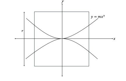
Figure 1. Level sets for $\det D^{2}u(x,y)$

By the homogeneity and symmetries of $u$, we have

$$\det D^{2}u(x,y)=\det D^{2}u(|x||y|^{-\frac{1}{\gamma}},1)$$

for all $y\neq 0.$ We recall from [2] that $g$ is equal to $c+dt^{2}$ for small $|t|$ and some $c,d>0$.

For $m>0$ large to be chosen shortly, we let $A_{r}$ be the region in $R_{r}$ that either lies above $y=m|x|^{\gamma}$ or below $y=-m|x|^{\gamma}$. In $A_{r}$, we have $|t|<m^{-\frac{1}{\gamma}}$. Choose $m$ large, so that $g(t)=c+dt^{2}$ inside the region $A_{r}$.

Now for $(x,y)=(x,1)$, we have $t=x$. Thus ,

$$\det(D^{2}u(x,1)) =\gamma^{-2}2d\left((\gamma+1)(c+dx^{2})+2d(\gamma-1)x^{2}\right)+4d^{2}x^{2}$$

$$=\frac{2cd(\gamma+1)}{\gamma^{2}}+\frac{2d^{2}}{\gamma^{2}}(2\gamma^{2}+3\gamma-1)x^{2}$$

$$=a+bx^{2}$$

for $a:=\frac{2cd(\gamma+1)}{\gamma^{2}}$ and $b:=\frac{2d^{2}}{\gamma^{2}}(2\gamma^{2}+3\gamma-1)$. Thus, in the region $A_{r}$

$$\det(D^{2}u(x,y))=\det(D^{2}u(|x||y|^{-\frac{1}{\gamma}},1))=a+bx^{2}|y|^{-\frac{2}{\gamma}}.$$

Now, for the complement of the region $A_{r}$ inside the rectangle $R_{r}$, $\det(D^{2}u)$ is bounded. For small positive $r$, we have

$$\frac{1}{r^{2}}\int_{R_{r}}|f-a|^{p}$$

$$=\frac{1}{r^{2}}\int_{R_{r}\setminus A_{r}}|f-a|^{p}+\frac{1}{r^{2}}\int_{A_{r}}|f-a|^{p}$$

$$\leq C\frac{1}{r^{2}}|A_{r}^{c}\cap R_{r}|+\frac{4}{r^{2}}\int_{0}^{r}\int_{mx^{\gamma}}^{r}b^{p}x^{2p}y^{-\frac{2p}{\gamma}}$$

$$\leq C\left(r^{\gamma-1}+r^{2p\left(1-\frac{1}{\gamma}\right)}\right).$$

We conclude that

$$\left(\frac{1}{r^{2}}\int_{R_{r}}|f-a|^{p}\right)^{\frac{1}{p}}\leq C(r^{2(1-\frac{1}{\gamma})}+r^{\frac{\gamma-1}{p}})\leq Cr^{\alpha}$$

for all $r>0$.

3. Key Lemmas

In this section we prove a few lemmas that will help us prove our main theorem. Define $T_{t}(x):=tT(x)+(1-t)x$. Let $\rho(t):=T_{t_{\#}}(\rho_{0})$ and $j(t):=T_{t}{{}_{\#}}\left[\left(T-Id\right)\rho_{0}\right]$. Note that $(\rho,j)$ satisfies the continuity equation, that is,

$$\partial_{t}\rho+\nabla\cdot j=0.$$

As $T$ is the optimal transport map, we have $(\rho,j)$ minimizes $\int\frac{1}{\rho}|j|^{2}$ among all choices $(\rho,j)$ such that $\rho(0)=\rho_{0}$, $\rho(1)=\rho_{1}$ and the pair satisfies the continuity equation (for a proof, see Theorem 8.1 in [4]). For a more complete discussion on the definition of $\rho$ and $j$, look at section 3.1 in [3].

First we want to prove an $L^{\infty}$ bound on the optimal transport map $T$. The proof of this remains the same as in [3]. From now on, by the notation $a\ll 1$, we mean there exists some small $\delta>0$ universal, such that if $a\leq\delta$, then the conclusions hold.

Lemma 3.1.

Let $T$ be the optimal transport map from $\rho_{0}$ to $\rho_{1}$. Assume $\rho_{0}\geq\frac{1}{C_{0}}$. Assume $\mathcal{E}\ll 1$. Then $\sup_{B_{\frac{3}{4}}}|T-x|+\sup_{B_{\frac{3}{4}}}|T^{-1}-x|\lesssim\mathcal{E}^{\frac{1}{n+2}}$. Moreover for all $t\in[0,1]$, we have $T_{t}(B_{\frac{1}{8}})\subset B_{\frac{3}{16}}$ and $T_{t}^{-1}(B_{\frac{1}{2}})\subset B_{\frac{3}{4}}$.

Proof.

Note that using the lower bound for $\rho_{0}$, it is enough to prove

$$\sup_{B_{\frac{3}{4}}}|T-x|+\sup_{B_{\frac{3}{4}}}|T^{-1}-x|\lesssim\int_{B_{1}}(|T-x|^{2})^{\frac{1}{n+2}}.$$

First we will show

$$\sup_{B_{\frac{3}{4}}}|T-x|\lesssim\int_{B_{1}}(|T-x|^{2})^{\frac{1}{n+2}}.$$

Define $v(x):=T(x)-x$. Use monotonicity of the optimal transport map to get for almost every $x,y\in B_{1}$,

(4) $$(v(x)-v(y))\cdot(x-y)\geq-|x-y|^{2}.$$

Let $y\in B_{\frac{3}{4}}$ be such that the above holds for a.e. $x$. Up to translation, we assume $y=0$. If $v_{1}$ denotes the first coordinate of $v$, then up to rotation all we need to show is

$$v_{1}(0)\lesssim\left(\int_{B_{\frac{1}{4}}}|u|^{2}\right)^{\frac{1}{n+2}}.$$

Put $y=0$ in (4), to conclude for a.e. $x\in B_{\frac{1}{4}}$, we have

$$v(0)\cdot x\leq v(x)\cdot x+|x|^{2}\lesssim|v(x)|^{2}+|x|^{2}.$$

Integrate the previous inequality over $B_{r}(re_{1})$ to get

$$v(0)\cdot re_{1}\lesssim\fint_{B_{r}(re_{1})}|v|^{2}+r^{2}.$$

This gives

$$v_{1}(0)\lesssim\frac{1}{r^{n+1}}\int_{B_{1}}|v|^{2}+r.$$

Optimize in $r$ to gives us the desired result for $T$.

If we run the above argument for $T$ in a ball of radius $\frac{4}{5}$ instead of in $B_{\frac{3}{4}}$, then it is enough to show $T^{-1}(B_{\frac{3}{4}})\subset B_{\frac{4}{5}}$. We prove this by contradiction. If this was false, there exists $y\in B_{\frac{3}{4}}$ and $x\notin B_{\frac{4}{5}}$ such that $T(x)=y$. Define $z$ to be the unique point in the line joining $x$ and $y$ such that $z\in\partial B_{\frac{1}{2}\left(\frac{3}{4}+\frac{4}{5}\right)}.$ Now by monotonicity of $T$, we have

$$0 \leq(T(x)-T(z))\cdot(x-z)$$

$$=(y-z)\cdot(x-z)+(z-T(z))\cdot(x-z)$$

$$\leq-\frac{1}{40}|x-z|+|x-z||T(z)-z|$$

$$\leq|x-z|\left(-\frac{1}{40}+\sup_{B_{\frac{1}{2}\left(\frac{3}{4}+\frac{4}{5}\right)}}|T-x|\right).$$

Using the $L^{\infty}$ bound for $T-x$, we get a contradiction to $\mathcal{E}\ll 1$ .

∎

In the next lemma we want to prove that our $\rho$ can not be arbitrarily far away from $1$. The idea is to use concavity of $\det^{\frac{1}{n}}$.

Lemma 3.2.

Assume $\mathcal{E}+||\rho_{0}||^{2}_{p,1}+||\rho_{1}||^{2}_{p,1}\ll 1$. Then $\rho(t)\leq C$ for some $C>0$ universal.

Proof.

For every $0<t<1$, $T_{t}$ has a well defined inverse a.e.(see Theorem 8.1 in [4]). This means for $x\in B_{1}$, we have

$$\rho(t,x)=\frac{\rho_{0}(T_{t}^{-1}(x))}{\det\nabla T_{t}(T_{t}^{-1}(x))}.$$

Concavity of $\det^{\frac{1}{n}}$ on symmetric matrices gives us $\det\nabla T_{t}(T_{t}^{-1}(x))\geq(\det\nabla T(T_{t}^{-1})(x))^{t}$. We also know

$$\det\nabla T(T_{t}^{-1}(x))=\frac{\rho_{0}(T_{t}^{-1}(x))}{\rho_{1}(T(T_{t}^{-1}(x)))}.$$

Conclude that

$$\rho(t,x)\leq\frac{\rho_{0}(T_{t}^{-1}(x))}{(\det\nabla T(T_{t}^{-1}(x)))^{t}}\leq(\rho_{0}(T_{t}^{-1}(x)))^{1-t}(\rho_{1}(T(T_{t}^{-1}(x))))^{t}.$$

As both $\rho_{0}$ and $\rho_{1}$ is bounded, we are done. ∎

The term $||\rho_{0}||_{p,1}+||\rho_{1}||_{p,1}$ arises a lot in this paper. From now on, we denote $\gamma:=||\rho_{0}||_{p,1}+||\rho_{1}||_{p,1}$. Next, we show that the interpolation density $\rho(t,x)$ is close to $1$ in the ball of radius $\frac{1}{2}$ in $L^{1}$ sense.

Lemma 3.3.

For $\mathcal{E}+||\rho_{0}||^{2}_{p,1}+||\rho_{1}||^{2}_{p,1}\ll 1$, we have

$$\int_{0}^{1}\int_{B_{\frac{1}{2}}}|\rho-1|dx\>dt\lesssim\mathcal{E}^{\frac{1}{n+2}}+\sqrt{\gamma}.$$

Proof.

First using concavity of $\log\det,$ conclude that $\det(\nabla T_{t})\geq\rho_{0}^{t}.$ Now,

$$\int_{0}^{1}\int_{B_{\frac{1}{2}}}|\rho-1|dx\;dt =\int_{0}^{1}\int_{B_{\frac{1}{2}}}\left|\frac{\rho_{0}(T_{t}^{-1}(x))}{\det(\nabla T_{t}(T_{t}^{-1}(x)))}-1\right|dx\;dt$$

$$=.\int_{0}^{1}\int_{T_{t}^{-1}(B_{\frac{1}{2}})}\left|\frac{\rho_{0}(z)}{\det(\nabla T_{t}(z))}-1\right|\det(\nabla T_{t}(z))dz\;dt$$

$$=\int_{0}^{1}\int_{T_{t}^{-1}(B_{\frac{1}{2}})}|\rho_{0}(z)-\det(\nabla T_{t}(z))|dz\;dt.$$

Thus, to finish the proof, all we need to show is

$$\int_{0}^{1}\int_{T_{t}^{-1}(B_{\frac{1}{2}})}|\rho_{0}(x)-\det(\nabla T_{t}(x))|dx\;dt\lesssim\mathcal{E}^{\frac{1}{n+2}}+\sqrt{\gamma}.$$

By triangle inequality,

$$\int_{0}^{1}\int_{T_{t}^{-1}(B_{\frac{1}{2}})}|\rho_{0}(x)-\det(\nabla T_{t}(x))|dx\;dt$$

$$\leq\int_{0}^{1}\int_{T_{t}^{-1}(B_{\frac{1}{2}})}|\rho_{0}(x)-1|dx\;dt+\int_{0}^{1}\int_{T_{t}^{-1}(B_{\frac{1}{2}})}|\det(\nabla T_{t}(x))-1|dx\;dt.$$

As by the previous lemma, $T_{t}^{-1}(B_{\frac{1}{2}})\subset B_{1}$, the first term of the right hand side is bounded by $C\gamma$ for some constant $C$ depending only on dimension. To bound the second term, we use that $\det(\nabla T_{t})\geq\rho_{0}^{t}$ for all $t$:

$$\int_{0}^{1}\int_{T_{t}^{-1}(B_{\frac{1}{2}})}|\det(\nabla T_{t}(x))-1|dx\;dt$$

$$\leq\int_{0}^{1}\int_{A_{t}}\left(1-\det(\nabla T_{t}(x))\right)dx\;dt+\int_{0}^{1}\int_{A_{t}^{c}}\left|1-\det(\nabla T_{t}(x)\right)|dx\;dt,$$

where $A_{t}:=T_{t}^{-1}(B_{\frac{1}{2}})\cap\{\rho_{0}^{t}\leq\det(\nabla T_{t})\leq(1-\sqrt{\gamma})^{t}\}$ and $A_{t}^{c}$ be the complement of $A_{t}$ inside $T_{t}^{-1}(B_{\frac{1}{2}}).$ We show that measure of $A_{t}$ can not be too big:

$$|A_{t}| \leq T_{t}^{-1}(B_{\frac{1}{2}})\cap\{\rho_{0}\leq 1-\sqrt{\gamma}\}$$

$$\leq T_{t}^{-1}(B_{\frac{1}{2}})\cap\{|\rho_{0}-1|\geq\sqrt{\gamma}\}$$

$$\leq\gamma^{\frac{-p}{2}}\int_{T_{t}^{-1}(B_{\frac{1}{2}})}|\rho_{0}-1|^{p}dx$$

$$\lesssim\gamma^{\frac{p}{2}},$$

where we have used Chebyshev’s inequality for the third step above. Hence,

$$\int_{0}^{1}\int_{A_{t}}\left(1-\det(\nabla T_{t}(x))\right)dx\;dt\leq\int_{0}^{1}|A_{t}|\leq\gamma^{\frac{p}{2}}\leq\sqrt{\gamma}.$$

To finish the proof, all we need to show is

$$\int_{0}^{1}\int_{A_{t}^{c}}\left|1-\det(\nabla T_{t}(x)\right)|dx\;dt\lesssim\mathcal{E}^{\frac{1}{n+2}}+\sqrt{\gamma}.$$

Now,

$$\int_{0}^{1}\int_{A_{t}^{c}}\left|1-\det(\nabla T_{t}(x)\right)|dx\;dt$$

$$\leq\int_{0}^{1}\int_{A_{t}^{c}}(\det(\nabla T_{t}(x))-1+2(1-(1-\sqrt{\gamma})^{t})dx\;dt.$$

As $(1-(1-\sqrt{\gamma})^{t})\leq\sqrt{\gamma}$ for all $t$, it is enough to show:

$$\int_{0}^{1}\int_{A_{t}^{c}}(\det(\nabla T_{t}(x))-1)dx\;dt\lesssim\sqrt{\gamma}+\mathcal{E}^{\frac{1}{n+2}}.$$

We have,

$$\int_{0}^{1}\int_{A_{t}^{c}}(\det(\nabla T_{t}(x))-1)dx\;dt$$

$$=\int_{0}^{1}\int_{A_{t}^{c}}\det(\nabla T_{t}(x))dx\;dt-\int_{0}^{1}\int_{A_{t}^{c}}1dx\;dt$$

$$\leq\int_{0}^{1}\int_{T_{t}^{-1}(B_{\frac{1}{2}})}\det(\nabla T_{t}(x))dx\;dt-|A_{t}^{c}|$$

$$=\int\int_{B_{\frac{1}{2}}}dz\;dt-|A_{t}^{c}|$$

$$=|B_{\frac{1}{2}}|-|A_{t}^{c}|.$$

We already know that $|A_{t}|\leq C\gamma^{\frac{p}{2}}$. Hence,

$$|A_{t}^{c}|=|T_{t}^{-1}(B_{\frac{1}{2}})|-|A_{t}|\geq|T_{t}^{-1}(B_{\frac{1}{2}})|-C\gamma^{\frac{p}{2}}\geq|B_{\frac{1}{2}-C\mathcal{E}^{\frac{1}{n+2}}}|-C\gamma^{\frac{p}{2}}$$

where we use Lemma 3.1 in the last inequality. Thus,

$$\int_{0}^{1}\int_{A_{t}^{c}}(\det(\nabla T_{t}(x))-1)dx\;dt\leq|B_{\frac{1}{2}}|-|B_{\frac{1}{2}-C\mathcal{E}^{\frac{1}{n+2}}}|+C\gamma^{\frac{p}{2}}$$

$$\lesssim\mathcal{E}^{\frac{1}{n+2}}+\gamma^{\frac{p}{2}}.$$

This completes the proof. ∎

Next, using convex analysis we want to show an $L^{2}$ to $L^{\infty}$ type estimate:

Lemma 3.4.

Let $Q(x)=|x|^{2}/2$ . If $\fint_{B_{1}}|\tilde{u}(x)-Q(x)|^{2}\lesssim\delta^{2}$ and $\tilde{u}$ is convex, then $|\tilde{u}-Q|\lesssim\delta^{\mu}$ in $B_{\frac{1}{2}}$, where $\mu=\frac{4}{4+n}$.

Proof.

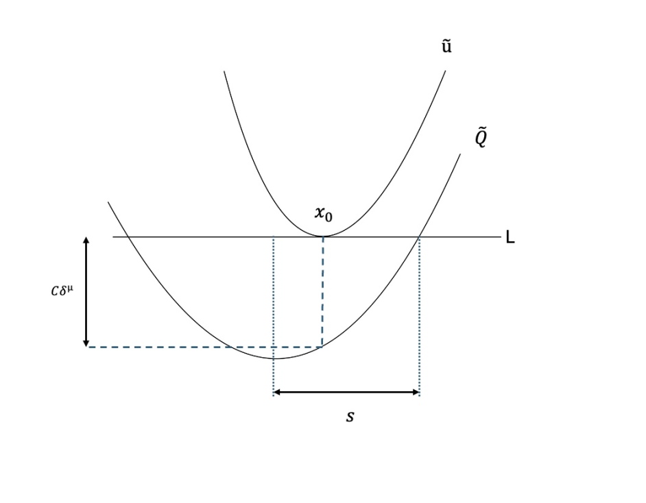
Figure 2. $u$ lies above $Q$

Suppose the theorem is false. Now we divide the proof into two cases. First let us assume $\tilde{u}(x_{0})-Q(x_{0})\geq C\delta^{\mu}$, that is $\tilde{u}$ lies above $Q$ (see Figure 2), for some large $C$ to be fixed later and for some $x_{0}\in B_{\frac{1}{2}}$. Up to subtracting a linear function we may assume $\nabla\tilde{u}(x_{0})=0$ (see Figure 2). Let $\tilde{Q}$ be $Q$ minus said linear function. Let $B:=\{x:\tilde{Q}(x)<\tilde{u}(x_{0})\}$ be the ball where $\tilde{Q}$ lies below the tangent of $\tilde{u}$ at $x_{0}$. Define $s$ to be the radius of the ball $B$. Because $\tilde{Q}=\frac{|x|^{2}}{2}$ up to adding a linear function, we have $s\geq C^{1/2}\delta^{\frac{\mu}{2}}$. Now,

$$\int_{B_{1}}|\tilde{u}-\tilde{Q}|^{2}\geq\int_{B}|\tilde{u}(x_{0})-\tilde{Q}|^{2}\geq c(n)C^{\frac{n+4}{2}}\delta^{\frac{4+n}{2}\mu}=c(n)C^{\frac{n+4}{2}}\delta^{2},$$

a contradiction for $C$ large.

In the second case, we assume $Q(x_{0})-\tilde{u}(x_{0})\geq C\delta^{\mu}$ ($Q$ lies above $\tilde{u}$) for some large $C$ to be fixed later (see Figure 3). Let $\tilde{Q}$ be $Q$ plus an affine function chosen such that $\nabla\tilde{Q}(x_{0})=0$. Add the same linear to $\tilde{u}$ and continue to denote it the same way. As $\fint_{B_{1}}|\tilde{u}(x)-\tilde{Q}(x)|^{2}\lesssim\delta^{2}$ , we know $\tilde{u}$ must cross the tangent hyperplane of $\tilde{Q}$ at $x_{0}$ at least at one point $x_{1}$ such that $|x_{1}-x_{0}|\leq\delta^{\frac{\mu}{2}}$. Indeed, if this was false, arguing in a similar way as in the first case and using the convexity of $\tilde{u}$ we will have

$$\int_{B_{1}}|\tilde{u}-\tilde{Q}|^{2}\geq\int_{B_{\delta^{\frac{\mu}{2}}}(x_{0})}\left(\tilde{Q}(x_{0})-\tilde{u}\right)^{2}\geq c(n)C^{2}\delta^{2},$$

a contradiction for $C$ large.
Consider the supporting hyperplane of $\tilde{u}$ at $x_{1}$. Call it $L$. From the above we know that $S:=|\nabla L|\geq C\delta^{\mu/2}$. It is elementary to show that

$$\max(L-\tilde{Q})=S^{2}/2+\nabla L\cdot(x_{0}-x_{1})\geq S(S/2-\delta^{\mu/2})\geq S^{2}/4,$$

provided $C>4$, hence

$$\max(L-\tilde{Q})\geq C^{2}\delta^{\mu}/4.$$

Using that $\tilde{u}\geq L$, taking $B=\{L>\tilde{Q}\}$ and arguing as in the first case, we are done.

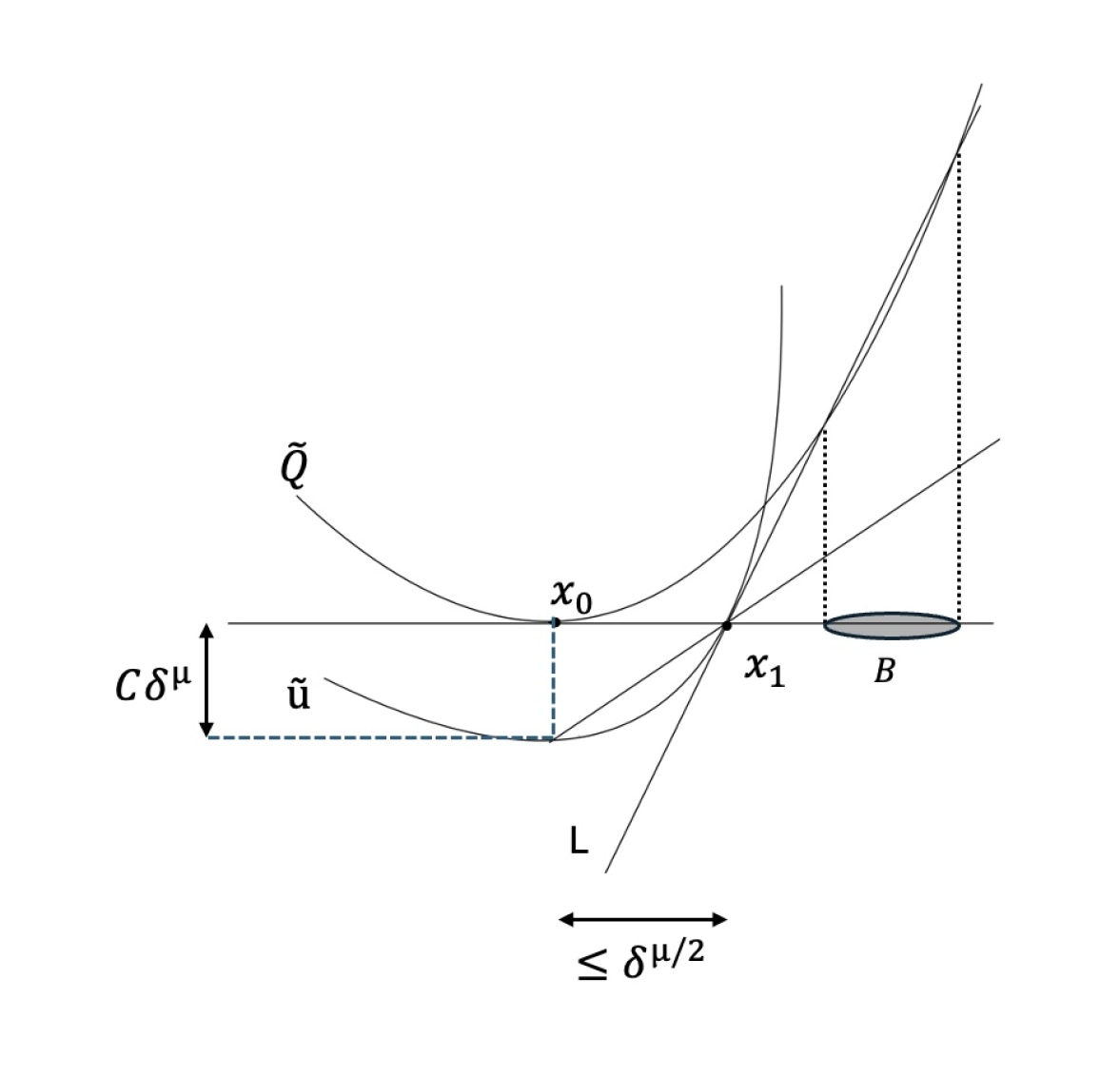
Figure 3. $u$ lies below $Q$

∎

4. Harmonic Approximation

Recall $\rho(t)=T_{t_{\#}}(\rho_{0})$ and $j(t):=T_{t_{\#}}\left[\left(T-Id\right)\rho_{0}\right]$, where $T_{t}(x):=tT(x)+(1-t)x$. Here we prove that the derivation of the velocity vector field $v:=\frac{\partial j}{\partial\rho}$ can be well approximated by gradient of some harmonic function if the excess energy is low and the densities $\rho_{0}$ and $\rho_{1}$ are close to uniform density.

Theorem 4.1.

Let $\mathcal{E}\ll 1$ and $\gamma\ll 1$ . Then there exists a harmonic function $\phi$ such that

(5) $$\int_{B_{\frac{1}{2}}}|\nabla\phi|^{2}\lesssim\int_{0}^{1}\int_{B_{1}}\frac{1}{\rho}|j|^{2}+\gamma^{2},$$

and

(6) $$\int_{0}^{1}\int_{B_{\frac{1}{2}}}\frac{1}{\rho}|j-\rho\nabla\phi|^{2}\lesssim\left(\int_{0}^{1}\int_{B_{1}}\frac{1}{\rho}|j|^{2}\right)^{\frac{n+2}{n+1}}+\gamma^{2}+\mathcal{E}^{\frac{1}{n+2}}\int_{0}^{1}\int_{B_{1}}\frac{1}{\rho}|j|^{2}.$$

Proof.

Without loss of generality assume $\int\int\frac{1}{\rho}|j|^{2}\ll 1,$ as otherwise we can just take $\phi=0$.
First we want to choose a good radius $R$ for which we can control the flux of $j$ through $\partial B_{R}$.
Use Fubini’s theorem and $\rho\leq C$ for some $C>0$ as proved in Lemma (3.2) to conclude

$$\int_{R=\frac{1}{2}}^{1}\int_{\partial B_{R}}\int_{0}^{1}|j|^{2}=\int_{B_{1}\setminus B_{\frac{1}{2}}}\int_{0}^{1}|j|^{2}\lesssim\int_{0}^{1}\int_{B_{1}}\frac{1}{\rho}|j|^{2}.$$

Thus we can find a good radius $R$ with $\frac{1}{2}<R<1$ such that

(7) $$\int_{\partial B_{R}}\int_{0}^{1}|j|^{2}\lesssim\int_{0}^{1}\int_{B_{1}}\frac{1}{\rho}|j|^{2}.$$

Using the inequality for every $\zeta\in H^{1}(B_{R}\times(0,1))$, we have

(8) $$\int_{0}^{1}\int_{B_{R}}\rho\partial_{t}\zeta+j\cdot\nabla\zeta=\int_{0}^{1}\int_{\partial B_{R}}\zeta f+\int_{B_{R}}\zeta(\cdot,1)\rho_{1}-\zeta(\cdot,0)\rho_{0}$$

where $f:=j\cdot\nu$ be the normal component of $j$. For a proof, look at the paragraph after equation 3.20 in [3].

Now we want to define our harmonic approximation $\phi$ whose gradient well approximates $\frac{\partial j}{\partial\rho}$. Let $\phi$ be the solution to

$$\begin{cases}-\Delta\phi=0\quad\text{in }\;\;B_{R}\\ \frac{\partial\phi}{\partial\nu}=\overline{f}+\frac{1}{\mathcal{H}^{d-1}(\partial B_{R})}\int_{B_{R}}\delta\rho\quad\text{on}\;\;\partial B_{R},\end{cases}$$

where $\overline{f}:=\int_{0}^{1}fdt$ and $\delta\rho:=\rho_{1}-\rho_{0}$. Applying (8) with $\zeta=1$ gives $\int_{B_{R}}\delta\rho=-\int_{\partial B_{R}}\overline{f}$. This shows we can solve for $\phi$.
Let us establish (5). Apply equation 2.2 from Lemma 2.1 in [3] with radius $R$ replaced by $R\sim 1$ to get

(9) $$\int_{B_{\frac{1}{2}}}|\nabla\phi|^{2} \leq\int_{B_{R}}|\nabla\phi|^{2}\lesssim\int_{\partial B_{R}}|\overline{f}|^{2}+||\delta\rho||^{2}_{L^{1}(B_{R})}\lesssim\int_{\partial B_{R}}|\overline{f}|^{2}+||\delta\rho||^{2}_{p,R}$$

$$\leq\int_{\partial B_{R}}\int_{0}^{1}|j|^{2}+||\delta\rho||^{2}_{p,R}\leq\int_{0}^{1}\int_{B_{1}}\frac{1}{\rho}|j|^{2}+\gamma^{2}.$$

This proves (5). We can in fact conclude something even better if use equation 2.3 from Lemma 2.1 in [3]. We will have

(10) $$||\nabla\phi||_{L^{\infty}(B_{\frac{1}{2}})}^{2}\leq\int_{B_{R}}|\nabla\phi|^{2}\lesssim\int_{0}^{1}\int_{B_{1}}\frac{1}{\rho}|j|^{2}+\gamma^{2}.$$

Now let us define $\tilde{\phi}$ and $\hat{\phi}$ as following:

$$\begin{cases}-\Delta\tilde{\phi}=\delta\rho\quad\text{in }\;\;B_{R}\\ \frac{\partial\tilde{\phi}}{\partial\nu}=\overline{f}\quad\text{on}\;\;\partial B_{R},\end{cases}$$

and

$$\begin{cases}-\Delta\hat{\phi}=\delta\rho\quad\text{in }\;\;B_{R}\\ \frac{\partial\tilde{\phi}}{\partial\nu}=-\frac{1}{\mathcal{H}^{d-1}(\partial B_{R})}\int_{B_{R}}\delta\rho\quad\text{on}\;\;\partial B_{R}.\end{cases}$$

Note that $\tilde{\phi}=\phi+\hat{\phi}$. We will show that it is enough to establish

(11) $$\int_{0}^{1}\int_{B_{R}}\frac{1}{\rho}|j-\rho\tilde{\phi}|^{2}\lesssim\left(\int_{0}^{1}\int_{B_{1}}\frac{1}{\rho}|j|^{2}\right)^{\frac{n+2}{n+1}}+\gamma^{2}+\mathcal{E}^{\frac{1}{n+2}}\int\int\frac{1}{\rho}|j|^{2},$$

and

(12) $$||\nabla\tilde{\phi}||^{2}_{L^{\infty}(B_{\frac{1}{2}})}\lesssim\int_{B_{R}}|\nabla\tilde{\phi}|^{2}\lesssim\int_{0}^{1}\int_{B_{R}}\frac{1}{\rho}|j|^{2}+\gamma^{2}.$$

Moreover, for $0<r\ll 1$, if we define $A_{r}:=B_{R}\setminus B_{R(1-r)}$, then

(13) $$\int_{A_{r}}|\nabla\tilde{\phi}|^{2}\lesssim r\left(\int_{\partial B_{R}}|\overline{f}|^{2}+\gamma^{2}\right).$$

Let’s now establish (12). For that we claim that

(14) $$||\nabla\hat{\phi}||_{L^{\infty}(B_{1})}\lesssim\gamma.$$

First let us prove this claim. Using global Calderón–Zygmund estimate(e.g. refer to [5]), we get $||D^{2}\hat{\phi}||_{L^{p}(B_{1})}\lesssim\gamma$. By Poincaré inequality, we have

$$||\nabla\hat{\phi}-\fint_{B_{1}}\nabla\hat{\phi}||_{L^{p}(B_{1})}\leq||D^{2}\hat{\phi}||_{L^{p}(B_{1})}\lesssim\gamma.$$

Conclude

$$||\nabla\hat{\phi}-\fint_{B_{1}}\nabla\hat{\phi}||_{W^{1,p}(B_{1})}=||\nabla\hat{\phi}-\fint_{B_{1}}\nabla\hat{\phi}||_{L^{p}(B_{1})}+||D^{2}\hat{\phi}||_{L^{p}(B_{1})}\lesssim\gamma.$$

By Morrey embedding theorem we have $W^{1,p}(B_{1})\subset C^{\alpha}(\overline{B_{1}})$. Thus,

(15) $$|\nabla\hat{\phi}-\fint_{B_{1}}\nabla\hat{\phi}|\leq C\gamma$$

pointwise for all $x\in\overline{B_{1}}$.
Suppose our claim was false. That means for any $C$ we can find $x_{0}\in\overline{B_{1}}$ such that $|\nabla\hat{\phi}(x_{0})|\geq C\gamma$. This with (15) gives $|\fint_{B_{1}}\nabla\hat{\phi}|\geq C\gamma$ for the same $C$. Conclude $|\nabla\hat{\phi}|\geq C\gamma$ at all points $x\in\overline{B_{1}}.$
We showed $\nabla\hat{\phi}$ blows up at all points on the boundary. Take $x_{1}\in\partial B_{1}$ such that $\hat{\phi}$ achieves its maximum on $\partial B_{1}$ at $x_{1}$. Hence, $\frac{\partial\hat{\phi}}{\partial T}=0$ where $T$ denotes the tangent direction. Thus, $\frac{\partial\hat{\phi}}{\partial\nu}$ must blow up. This is a contradiction to the Neumann Boundary condition we assumed in the definition of $\hat{\phi}$. This completes the proof of our claim.

This claim along with (10) immediately gives us (12) by triangle inequality. Similarly if we use equation 2.4 from [3] and Global Calderón–Zygmund estimate((see [5])), we can get (13).

Next we assume (11) and prove (6). Note that

$$\int_{0}^{1}\int_{B_{R}}\frac{1}{\rho}|j-\rho\nabla\phi|^{2}=\int_{0}^{1}\int_{B_{R}}\frac{1}{\rho}|j-\rho\nabla\tilde{\phi}+\rho\nabla\hat{\phi}|^{2}$$

$$\lesssim\int_{0}^{1}\int_{B_{R}}\frac{1}{\rho}|j-\rho\nabla\tilde{\phi}|^{2}+\int_{0}^{1}\int_{B_{R}}\rho|\nabla\hat{\phi}|^{2}.$$

The first term is bounded by (11). Use Lemma (3.2) and our previous claim to bound the second term:

$$\int_{0}^{1}\int_{B_{R}}\rho|\nabla\hat{\phi}|^{2}\lesssim\gamma^{2}.$$

This completes the proof, except we have not proved equation (11).

From now on, up to rescaling, assume $R=\frac{1}{2}$. Here we prove that

(16) $$\int_{0}^{1}\int_{B_{\frac{1}{2}}}\frac{1}{\rho}|j-\rho\tilde{\phi}|^{2}\lesssim\int_{0}^{1}\int_{B_{\frac{1}{2}}}\frac{1}{\rho}|j|^{2}-\int_{0}^{1}\int_{B_{\frac{1}{2}}}(2-\rho)|\nabla\tilde{\phi}|^{2}.$$

We have

$$\frac{1}{2}\int_{0}^{1}\int_{B_{\frac{1}{2}}}\frac{1}{\rho}|j-\rho\nabla\tilde{\phi}|^{2} =\frac{1}{2}\int_{0}^{1}\int_{B_{\frac{1}{2}}}\frac{1}{\rho}|j|^{2}-\int_{0}^{1}\int_{B_{\frac{1}{2}}}j\cdot\nabla\tilde{\phi}+\frac{1}{2}\int_{0}^{1}\int_{B_{\frac{1}{2}}}\rho|\nabla\tilde{\phi}|^{2}$$

$$=\frac{1}{2}\int_{0}^{1}\int_{B_{\frac{1}{2}}}\frac{1}{\rho}|j|^{2}-\int_{0}^{1}\int_{B_{\frac{1}{2}}}\left(1-\frac{\rho}{2}\right)|\nabla\tilde{\phi}|^{2}$$

$$-\int_{0}^{1}\int_{B_{\frac{1}{2}}}(j-\nabla\tilde{\phi})\cdot\nabla\tilde{\phi}.$$

Note that if we put $\zeta=\tilde{\phi}$ in (8), we have the last term to be zero. Hence we get (16).

In the final part of this proof, we establish that

(17) $$\int_{0}^{1}\int_{B_{\frac{1}{2}}}\frac{1}{\rho}|j|^{2}-\int_{B_{\frac{1}{2}}}|\nabla\tilde{\phi}|^{2}\lesssim\left(\int_{0}^{1}\int_{B_{1}}\frac{1}{\rho}|j|^{2}\right)^{\frac{n+2}{n+1}}+\gamma^{2}.$$

First we show this (17) along with (16) will give us (11):

(18) $$\int_{0}^{1}\int_{B_{\frac{1}{2}}}\frac{1}{\rho}|j-\rho\nabla\tilde{\phi}|^{2} \lesssim\int_{0}^{1}\int_{B_{\frac{1}{2}}}\frac{1}{\rho}|j|^{2}-\int_{0}^{1}\int_{B_{\frac{1}{2}}}(2-\rho)|\nabla\tilde{\phi}|^{2}$$

$$\lesssim\left(\int_{0}^{1}\int_{B_{1}\frac{1}{\rho}}|j|^{2}\right)^{\frac{n+2}{n+1}}+\gamma^{2}-\int_{0}^{1}\int_{B_{\frac{1}{2}}}(1-\rho)|\nabla\tilde{\phi}|^{2}$$

Note that to get (11) it is enough to prove

$$\left|\int_{0}^{1}\int_{B_{\frac{1}{2}}}(1-\rho)|\nabla\tilde{\phi}|^{2}\right|\lesssim\left(\int_{0}^{1}\int_{B_{1}}\frac{1}{\rho}|j|^{2}\right)^{\frac{n+2}{n+1}}+\gamma^{2}+\mathcal{E}^{\frac{1}{n+2}}\int\int\frac{1}{\rho}|j|^{2}.$$

We do this by using (12), Lemma 3.3 and Young’s inequality:

$$\left|\int_{0}^{1}\int_{B_{\frac{1}{2}}}(1-\rho)|\nabla\tilde{\phi}|^{2}\right|\lesssim||\nabla\tilde{\phi}||_{{}_{\infty}}^{2}\int\int_{B_{\frac{1}{2}}}|\rho-1|\lesssim\left(\sqrt{\gamma}+\mathcal{E}^{\frac{1}{n+2}}\right)\left(\int\int\frac{1}{\rho}|j|^{2}+\gamma^{2}\right)$$

$$\lesssim\left(\int_{0}^{1}\int_{B_{1}}\frac{1}{\rho}|j|^{2}\right)^{\frac{n+2}{n+1}}+\gamma^{2}+\mathcal{E}^{\frac{1}{n+2}}\int\int\frac{1}{\rho}|j|^{2}.$$

Thus all we need to prove is (17). By minimality of $(\rho,j)$, it is enough to construct a competitor $(\tilde{\rho},\tilde{j})$ that agrees with $(\rho,j)$ outside $B_{\frac{1}{2}}\times(0,1)$ and that satisfies the upper bound through (17).
We choose the following $(\tilde{\rho},\tilde{j})$

(19) $$(\tilde{\rho},\tilde{j})=\begin{cases}(t\rho_{1}+(1-t)\rho_{0},\nabla\tilde{\phi})\quad\text{in}\;\;B_{\frac{1}{2}(1-r)}\times(0,1)\\ (t\rho_{1}+(1-t)\rho_{0}+s,\nabla\tilde{\phi}+q)\quad\text{in}\;\;A_{r}\times(0,1),\end{cases}$$

with $(s,q)\in\Lambda$ where $\Lambda$ is defined in Lemma 2.4 from [3] with $f$ replaced by $f-\overline{f}$ and the radius $1$ replaced by radius $\frac{1}{2}$.
Note that if $|s|\leq\frac{1}{2C_{0}}$, then $\tilde{\rho}\geq\frac{1}{2C_{0}}$. In $B_{\frac{1}{2}(1-r)}$ we have $\tilde{\rho}\geq\frac{1}{2C_{0}}$ as both $\rho_{0}$ and $\rho_{1}$ are greater than $\frac{1}{C_{0}}$. In $A_{r}$, we have $\tilde{\rho}\geq\frac{1}{C_{0}}-\frac{1}{2C_{0}}\geq\frac{1}{2C_{0}}.$ Note that by definition of $\tilde{\phi}$, our choices for $(\tilde{\rho},\tilde{j})$ is admissible.
By Lemma 2.4 in [3](here we use a modified version of the Lemma: basically we take $|s|\leq\frac{1}{2C_{0}}$ instead of $|s|\leq\frac{1}{2}$ in the statement of the lemma), if

(20) $$r\gg\left(\int_{0}^{1}\int_{B_{\frac{1}{2}}}(f-\overline{f})^{2}\right)^{\frac{1}{n+1}},$$

we may choose $(s,q)\in\Lambda$ such that

(21) $$\int_{0}^{1}\int_{A_{r}}|q|^{2}\lesssim r\int_{0}^{1}\int_{\partial B_{\frac{1}{2}}}(f-\overline{f})^{2}.$$

By definition of $(\tilde{\rho},\tilde{j}),$

$$\int_{0}^{1}\int_{B_{\frac{1}{2}}}\frac{1}{\tilde{\rho}}|\tilde{j}|^{2}-\int_{B_{\frac{1}{2}}}|\nabla\tilde{\phi}|^{2}$$

$$\lesssim\int_{0}^{1}\int_{B_{\frac{1}{2}(1-r)}}\frac{1}{t\rho_{1}+(1-t)\rho_{0}}|\nabla(\tilde{\phi})|^{2}-\int_{B_{\frac{1}{2}(1-r)}}|\nabla(\tilde{\phi})|^{2}+\int_{0}^{1}\int_{A_{r}}\frac{1}{\tilde{\rho}}|\nabla\tilde{\phi}+q|^{2},$$

where we have replaced the second term in the RHS by an integration on a smaller domain.
The first two terms on RHS can be estimated as follows

$$\int_{0}^{1}\int_{B_{\frac{1}{2}(1-r)}}\left(\frac{1}{t\rho_{1}+(1-t)\rho_{0}}-1\right)|\nabla\tilde{\phi}|^{2} \lesssim\int_{0}^{1}\int_{B_{\frac{1}{2}}(1-t)}(1-t)(1-\rho_{0})|\nabla\tilde{\phi}|^{2}$$

$$\lesssim||\rho_{0}-1||_{L^{1}}||\nabla\tilde{\phi}||_{L^{\infty}}^{2}$$

$$\lesssim||\rho_{0}-1||_{L^{p}}||\nabla\tilde{\phi}||_{L^{\infty}}^{2}$$

$$\lesssim\gamma\left(\int\int\frac{1}{\rho}|j|^{2}+\gamma^{2}\right),$$

where in the first inequality we use $(1-t)\rho_{0}+t\rho_{1}$ is bounded from below in $B_{\frac{1}{2}(1-r)}$.
To estimate the last term use (21), (13) and (7) respectively

$$\int_{0}^{1}\int_{A_{r}}\frac{1}{\tilde{\rho}}|\nabla\tilde{\phi}+q|^{2} \lesssim\int_{0}^{1}\int_{A_{r}}|\nabla\tilde{\phi}|^{2}+|q|^{2}$$

$$\lesssim\int_{A_{r}}|\nabla\tilde{\phi}|^{2}+\int_{0}^{1}\int_{A_{r}}|q|^{2}$$

$$\lesssim\int_{A_{r}}|\nabla\tilde{\phi}|^{2}+r\int_{0}^{1}\int_{\partial B_{\frac{1}{2}}}(f-\overline{f})^{2}$$

$$\lesssim r\left(\int_{\partial B_{\frac{1}{2}}}\overline{f}^{2}+\gamma^{2}\right)+r\int_{0}^{1}\int_{\partial B_{\frac{1}{2}}}(f-\overline{f})^{2}$$

$$\lesssim r\left(\gamma^{2}+\int\int f^{2}\right)$$

$$\lesssim r\left(\gamma^{2}+\int\int\frac{1}{\rho}|j|^{2}\right)$$

Choose $r$ to be large multiple of (order one though) $\left(\int_{0}^{1}\int_{B_{\frac{1}{2}}}(f-\overline{f})^{2}\right)^{\frac{1}{n+1}}$ to make sure (21) holds. Note that,

$$\left(\int_{0}^{1}\int_{B_{\frac{1}{2}}}(f-\overline{f})^{2}\right)^{\frac{1}{n+1}} \lesssim 2\left(\int_{0}^{1}\int_{\partial B_{\frac{1}{2}}}f^{2}+\int_{\partial B_{\frac{1}{2}}}\overline{f}^{2}\right)^{\frac{1}{n+1}}\lesssim\left(\int\int f^{2}\right)^{\frac{1}{n+1}}$$

$$\lesssim\left(\int\int\frac{1}{\rho}|j|^{2}\right)^{\frac{1}{n+1}},$$

where we use (7) to get the last inequality.
Combining last two calculations, if we denote $a=\int\int\frac{1}{\rho}|j|^{2}$, then by Young’s inequality we have

$$\int_{0}^{1}\int_{B_{\frac{1}{2}}}\frac{1}{\tilde{\rho}}|\tilde{j}|^{2}-\int_{B_{\frac{1}{2}}}|\nabla\tilde{\phi}|^{2} \lesssim\gamma(a+\gamma^{2})+a^{\frac{1}{n+1}}(a+\gamma^{2})$$

$$\lesssim(\gamma+a^{\frac{1}{n+1}})(a+\gamma^{2})=a^{\frac{n+2}{n+1}}+a\gamma+a^{\frac{1}{n+1}}\gamma^{2}+\gamma^{2}$$

$$\lesssim a^{\frac{n+2}{n+1}}+\gamma^{2}.$$

This finish the proof of equation (17) and we are done. ∎

Taking motivation from the theory of minimal surface equations , next we want to prove that $T-x$ is well approximated by $\nabla\phi$.

Lemma 4.2.

Let $T$ be the optimal transport map that takes the density $\rho_{0}$ to $\rho_{1}$. Then there is a harmonic map $\phi$ in $B_{\frac{1}{8}}$ such that

(22) $$\int_{B_{\frac{1}{8}}}|T-x-\nabla\phi|^{2}\rho_{0}\lesssim\mathcal{E}^{\frac{n+3}{n+2}}+\gamma^{2},$$

and

(23) $$\int_{B_{\frac{1}{8}}}|\nabla\phi|^{2}\lesssim\mathcal{E}+\gamma^{2}.$$

Proof.

First note that we may assume $\mathcal{E}+\gamma^{2}\ll 1$ since otherwise we can take $\phi=0$. We know that the velocity vector field $v:=\frac{\partial j}{\partial\rho}$ satisfies $v(T_{t}(x),t)=T(x)-x$ for a.e. $x\in supp(\rho_{0})$ (see for example Theorem 8.1 in [4]). Thus, using (3.1) we have:

(24) $$\int_{0}^{1}\int_{B_{\frac{1}{2}}}\frac{1}{\rho}|j|^{2} =\int_{0}^{1}\int_{B_{\frac{1}{2}}}|v|^{2}\;d\rho$$

$$\lesssim\int_{0}^{1}\int_{T_{t}^{-1}(B_{\frac{1}{2}})}|T(x)-x|^{2}\rho_{0}dx$$

$$\lesssim\int_{0}^{1}\int_{B_{1}}|T-x|^{2}\rho_{0}$$

$$=\mathcal{E}.$$

By Lemma 4.1, we can find a harmonic function $\phi$ in $B_{\frac{1}{4}}$ such that

(25) $$\int_{B_{\frac{1}{4}}}|\nabla\phi|^{2}\lesssim\int_{0}^{1}\int_{B_{1}}\frac{1}{\rho}|j|^{2}+\gamma^{2},$$

and

(26) $$\int_{0}^{1}\int_{B_{\frac{1}{4}}}\frac{1}{\rho}|j-\rho\nabla\phi|^{2} \lesssim\left(\int_{0}^{1}\int_{B_{\frac{1}{2}}}\frac{1}{\rho}|j|^{2}\right)^{\frac{n+2}{n+1}}+\gamma^{2}+\mathcal{E}^{\frac{1}{n+2}}\int\int_{B_{\frac{1}{2}}}\frac{1}{\rho}|j|^{2}$$

$$\lesssim\mathcal{E}^{\frac{n+3}{n+2}}+\gamma^{2}.$$

For the second inequality above, we use (24). Using (24) and (25), we get (23).

Next we want to prove (22). By triangle inequality we have

(27) $$\int_{B_{\frac{1}{8}}}|T-(x+\nabla\phi)|^{2}\rho_{0}\lesssim\int_{0}^{1}\int_{B_{\frac{1}{8}}}|T-x+\nabla\phi\circ T_{t}|^{2}\rho_{0}+\int_{0}^{1}\int_{B_{\frac{1}{8}}}|\nabla\phi-\nabla\phi\circ T_{t}|^{2}\rho_{0}.$$

Recall $|T_{t}(x)-x|\leq|T(x)-x|$ for all $t$ by definition of $T_{t}$ and we use this to estimate the second term of the right hand side of (27):

$$\int_{0}^{1}\int_{B_{\frac{1}{8}}}|\nabla\phi-\nabla\phi\circ T_{t}|^{2}\rho_{0} \lesssim\sup_{B_{\frac{3}{16}}}|D^{2}\phi|^{2}\int_{0}^{1}\int_{B_{\frac{1}{8}}}|T_{t}-x|^{2}\rho_{0}$$

$$\lesssim\left(\int_{B_{\frac{1}{4}}}|\nabla\phi|^{2}\right)\mathcal{E}$$

$$\lesssim\mathcal{E}(\mathcal{E}+\gamma^{2}),$$

where we have used Lemma (3.1) and equation 2.3 in Lemma 2.1 in [3].
Recall $v:=\frac{\partial j}{\partial\rho}$ satisfies $v(T_{t}(x),t)=T(x)-x$. This means

$$T(x)-x-\nabla\phi(T_{t}(x))=v(T_{t}(x),t)-\nabla\phi(T_{t}(x))$$

$$\implies T(x)-(x+\nabla\phi(T_{t}(x)))=\left(v(t,\cdot)-\nabla\phi\right)(T_{t}(x))$$

which holds for a.e. $x\in supp(\rho_{0})$. Let’s now estimate the first term in the right hand side of (27) using (24) and (26):

$$\int_{0}^{1}\int_{B_{\frac{1}{8}}}|T-x+\nabla\phi\circ T_{t}|^{2}\rho_{0} =\int_{0}^{1}\int_{T_{t}(B_{\frac{1}{8}})}|v-\nabla\phi|^{2}d\rho$$

$$=\int_{0}^{1}\int_{T_{t}(B_{\frac{1}{8}})}\frac{1}{\rho}|j-\rho\nabla\phi|^{2}$$

$$\lesssim\int_{0}^{1}\int_{B_{\frac{1}{4}}}\frac{1}{\rho}|j-\rho\nabla\phi|^{2}$$

$$\lesssim\mathcal{E}^{\frac{n+3}{n+2}}+\gamma^{2}.$$

This completes the proof. ∎

5. One Step Improvement

Next we prove that if at a certain scale $R$, T is close to identity, that is if

$$\mathcal{E}+\left(||\rho_{0}||_{p,R}^{2}+||\rho_{1}||_{p,R}^{2}\right)\ll 1,$$

then on scale $R\theta$, after an affine change of coordinates, it is even closer to identity by a geometric factor. Together with (22) from Lemma 4.2, regularity result equation 2.3 from Lemma 2.1 in [3], we will have the proof.

Proposition 5.1.

For all $0<\alpha^{\prime}<1$ there exists $\theta(n,\alpha,\alpha^{\prime})>0$, $\epsilon(n,\alpha,\alpha^{\prime})>0$ and $C_{\theta}(n,\alpha,\alpha^{\prime})$ with the property that for all $R>0$ such that

(28) $$\mathcal{E}(\rho_{0},\rho_{1},T,R)+||\rho_{0}||_{p,R}^{2}+||\rho_{1}||_{p,R}^{2}\leq\epsilon$$

there exists symmetric matrix $B\in SL_{n}(\mathbb{R})$ and a vector $b$ such that if we let $\hat{x}:=B^{-1}x$, $\hat{y}:=B(y-b)$, $\hat{T}(\hat{x})=B(T(x)-b)$, $\hat{\rho_{0}}(\hat{x}):=\rho_{0}(x)$ and $\hat{\rho_{1}}(\hat{y})=\rho_{1}(y)$, then

$$\mathcal{E}(\hat{\rho_{0}},\hat{\rho_{1}},\hat{T},\theta R)\leq\theta^{2\alpha^{\prime}}\mathcal{E}(\rho_{0},\rho_{1},T,R)+C_{\theta}\left(||\rho_{0}||_{p,R}^{2}+||\rho_{1}||_{p,R}^{2}\right).$$

Moreover,

$$|B-Id|^{2}+\frac{1}{R^{2}}|b|^{2}\lesssim\mathcal{E}(\rho_{0},\rho_{1},T,R)+||\rho_{0}||_{p,R}^{2}+||\rho_{1}||_{p,R}^{2}.$$

Proof.

By rescaling we may assume $R=1$. For this proof, let $\mathcal{E}=\mathcal{E}(\rho_{0},\rho_{1},T,R=1)$. Let $\phi$ comes from Lemma 4.2. Define $b:=\nabla\phi(0)$, $A=\nabla^{2}\phi(0)$ and $B:=e^{-\frac{A}{2}}$. Clearly,

$$\det(B)=\det(e^{-\frac{A}{2}})=e^{-\frac{tr(A)}{2}}=e^{-\frac{\Delta\phi}{2}}=e^{0}=1$$

where we use $\Delta\phi=0$. Using equation 2.3 from Lemma 2.1 in [3] and Lemma 4.2

$$|B-Id|^{2}+|b|^{2}\lesssim\mathcal{E}(\rho_{0},\rho_{1},T,R)+||\rho_{0}||_{p,R}^{2}+||\rho_{1}||_{p,R}^{2}.$$

Now, we have

$$\fint_{B_{\theta}}|\hat{T}-\hat{x}|^{2}\rho_{0} =\fint_{B_{\theta}}|B(T(x)-b)-B^{-1}x|^{2}\rho_{0}$$

$$=\fint_{BB_{\theta}}|T(x)-(B^{-2}x+b)|^{2}\rho_{0}$$

$$\lesssim\fint_{B_{2\theta}}|T(x)-(B^{-2}x+b)|^{2}\rho_{0}$$

$$\lesssim\fint_{B_{2\theta}}|T(x)-(x+\nabla\phi)|^{2}\rho_{0}+\fint_{B_{2\theta}}|(B^{-2}-Id-A)x|^{2}\rho_{0}$$

$$+\fint_{B_{2\theta}}|\nabla\phi-b-Ax|^{2}\rho_{0}$$

$$\lesssim\fint_{B_{2\theta}}|T(x)-(x+\nabla\phi)|^{2}\rho_{0}+\theta^{2}|B^{-2}-Id-A|^{2}+$$

$$\sup_{B_{2\theta}}|\nabla\phi-b-Ax|^{2}$$

$$=\mathcal{I}+\mathcal{II}+\mathcal{III},$$

where

$$\mathcal{I}:=\fint_{B_{2\theta}}|T(x)-(x+\nabla\phi)|^{2}\rho_{0},$$

$$\mathcal{II}:=\theta^{2}|B^{-2}-Id-A|^{2},$$

and

$$\mathcal{III}:=\sup_{B_{2\theta}}|\nabla\phi-b-Ax|^{2}.$$

Now as per Lemma 4.2, we have the the first term

$$\mathcal{I}\lesssim\theta^{-n}\left(\mathcal{E}^{\frac{n+3}{n+2}}+\gamma^{2}\right).$$

The second term can be estimated using Taylor series expansion

$$|B^{-2}-Id-\nabla^{2}\phi(0)|^{2}=|e^{A}-Id-A|^{2}=\frac{|A|^{4}}{2}=\frac{|\nabla^{2}\phi(0)|^{4}}{2}.$$

Hence, $\mathcal{II}\lesssim\theta^{2}|\nabla^{2}\phi(0)|^{4}$.
Now ,

$$\sup_{B_{2\theta}}|\nabla\phi-b-Ax|^{2}=\sup_{B_{2\theta}}|f(x)-f(0)-\nabla f(0)x|^{2},$$

where $f(x)=\nabla\phi(x)$. Use Taylor series expansion for $\nabla\phi$, we get

$$\mathcal{III}\lesssim\sup_{B_{2\theta}}|x^{T}\nabla^{2}f(0)x|^{2}=\theta^{4}|\nabla^{3}\phi(0)|^{2}.$$

Combining and multiplying by $\theta^{-2}$ on both side,

$$\theta^{-2}\fint_{B_{\theta}}|\hat{T}-\hat{x}|^{2}\rho_{0} \lesssim\theta^{-(n+2)}\mathcal{E}^{\frac{n+2}{n+1}}+\theta^{-(n+2)}||\rho_{0}||_{p,1}^{2}+\theta^{-(n+2)}||\rho_{1}||_{p,1}^{2}+|\nabla^{2}\phi(0)|^{4}+\theta^{2}|\nabla^{3}\phi(0)|^{2}.$$

Now using equation 2.3 from [3] and (23), we have

$$|\nabla^{2}\phi(0)|^{4}\lesssim\left(\int_{B_{1}}|\nabla\phi|^{2}\right)^{2}\lesssim\left(\mathcal{E}+\gamma^{2}\right)^{2}.$$

Similarly, we will get

$$\theta^{2}|\nabla^{3}\phi(0)|^{2}\lesssim\theta^{2}\left(\mathcal{E}+\gamma^{2}\right).$$

Hence, we have

$$\theta^{-2}\fint_{B_{\theta}}|\hat{T}-\hat{x}|^{2}\rho_{0} \lesssim\theta^{-(n+2)}\mathcal{E}^{\frac{n+3}{n+2}}+\theta^{-(n+2)}\left(||\rho_{0}||_{p,1}^{2}+||\rho_{1}||_{p,1}^{2}\right)$$

$$+\left(\mathcal{E}+||\rho_{0}||_{p,1}^{2}+||\rho_{1}||_{p,1}^{2}\right)^{2}+\theta^{2}\left(\mathcal{E}+||\rho_{0}||_{p,1}^{2}+||\rho_{1}||_{p,1}^{2}\right).$$

As we have assumed $\mathcal{E}+||\rho_{0}||_{p,1}^{2}+||\rho_{1}||_{p,1}^{2}\ll 1$, we can absorb second term of RHS on the third term($\mathcal{E}+||\rho_{0}||_{p,1}^{2}+||\rho_{1}||_{p,1}^{2}<\theta^{2}$ as $\theta$ to be fixed).

$$\theta^{-2}\fint_{B_{\theta}}|\hat{T}-\hat{x}|^{2}\rho_{0} \lesssim\theta^{-(n+2)}\mathcal{E}^{\frac{n+3}{n+3}}+\theta^{-(n+2)}\left(||\rho_{0}||_{p,1}^{2}+||\rho_{0}||_{p,1}^{2}\right)$$

$$+\theta^{2}\left(\mathcal{E}+||\rho_{0}||_{p,1}^{2}+||\rho_{1}||_{p,1}^{2}\right).$$

Now we absorb the term with $\theta^{2}\left(||\rho_{0}||^{2}_{p,1}+||\rho_{1}||^{2}_{p,1}\right)$ in $\theta^{-(n+2)}\left(||\rho_{0}||_{p,1}^{2}+||\rho_{1}||^{2}_{p,1}\right)$ as $\theta$ to be chosen is small (less than 1):

$$\theta^{-2}\fint_{B_{\theta}}|\hat{T}-\hat{x}|^{2}\rho_{0}\leq C\theta^{-(n+2)}\mathcal{E}^{\frac{n+3}{n+2}}+C\theta^{-(n+2)}\left(||\rho_{0}||_{p,1}^{2}+||\rho_{1}||_{p,1}^{2}\right)+C\theta^{2}\mathcal{E}.$$

Next, fix $\theta$ small so that $C\theta^{2}\leq\frac{1}{2}\theta^{2\alpha^{\prime}}$. This is possible because $\alpha^{\prime}<1$. As we have $\mathcal{E}\ll 1$, conclude $C\theta^{-(n+2)}\mathcal{E}^{\frac{n+3}{n+2}}\leq\frac{1}{2}\theta^{2\alpha^{\prime}}\mathcal{E}$. Thus we get

$$\theta^{-2}\fint_{B_{\theta}}|\hat{T}-\hat{x}|^{2}\rho_{0}\leq\theta^{2\alpha^{\prime}}\mathcal{E}+C_{\theta}\left(||\rho_{0}||_{p,1}^{2}+||\rho_{1}||_{p,1}^{2}\right).$$

∎

6. $\epsilon$ Regularity

Now we want to iterate our previous step to get $\epsilon$ regularity:

Theorem 6.1.

Let $||\rho_{0}||_{p,r}\leq\sqrt{\epsilon_{1}}r^{\alpha}$ for all $r>0$ and

$$\mathcal{E}(\rho_{0},\rho_{1},T,R)+||\rho_{0}||_{p,R}^{2}+||\rho_{1}||_{p,R}^{2}\leq\epsilon_{1}$$

for some $\epsilon_{1}$ fixed. Then

$$\sup_{r\leq\frac{R}{2}}\min_{A,b}\frac{1}{r^{2(1+\alpha)}}\fint_{B_{r}(0)}|T-(Ax+b)|^{2}\lesssim R^{-2\alpha}\left(\mathcal{E}(\rho_{0},\rho_{1},T,R)+||\rho_{0}||^{2}_{p,R}+||\rho_{1}||^{2}_{p,R}\right).$$

Proof.

Without loss of generality assume $R=1$. Fix $\alpha^{\prime}>\alpha$. Fix $0<\theta<\frac{1}{8}$. Define $\mathcal{E}_{0}=\mathcal{E}(\rho_{0},\rho_{1},T,1)$ and $\rho_{i}^{0}=\rho_{i}$ for $i=1,2$. Let $\epsilon$ be as in Proposition 5.1.

Applying Proposition 5.1, we know that there exists a symmetric matrix $B_{1}\in SL_{n}(\mathbb{R})$ and a vector $b_{1}$ such that if wet let $T_{1}(x):=B_{1}\left(T(B_{1}x)-b_{1}\right)$, $\rho_{0}^{1}(x):=\rho_{0}(B_{1}x)$ and $\rho_{1}^{1}(y)=\rho_{1}(B_{1}^{-1}y+b_{1})$ then there exists $C_{0}>1$ satisfying

$$\mathcal{E}_{1}:=\mathcal{E}(\rho_{0}^{0},\rho_{1}^{0},T_{1},\theta)\leq\theta^{2\alpha^{\prime}}\mathcal{E}_{0}+C_{0}p_{0}^{2},$$

where $p_{0}^{2}=||\rho_{0}^{0}||^{2}_{p,1}+|||\rho_{1}^{0}||_{p,1}^{2}$ . Moreover $|B_{1}-Id|^{2}+|b_{1}|^{2}\leq C_{0}\left(\mathcal{E}_{0}+p_{0}^{2}\right)$.

Assuming we can keep applying Proposition 5.1 repetitively, let $\rho_{0}^{k}$ and $\rho_{1}^{k}$ are the new source and target densities respectively after applying Proposition 5.1 k times, that is, $\rho_{0}^{k}(x):=\rho_{0}^{k-1}(B_{k}x)$ and $\rho_{1}^{k}(x)=\rho_{1}^{k-1}\left(B_{k}^{-1}x+b_{k}\right),$ where $B_{k}\in SL_{n}(\mathbb{R})$ is symmetric and $b_{k}\in\mathbb{R}^{n}$. Let $T_{k}$ be the optimal transport map from $\rho_{0}^{k}$ and $\rho_{1}^{k}$. For all $k=0,1,\cdots$, define $\mathcal{E}_{k}:=\mathcal{E}(\rho_{0}^{k},\rho_{1}^{k},T_{k},\theta^{k})$ and for all $k=1,2,\cdots$, define $\tilde{B_{k}}=|B_{k}-Id|$ and $p_{k}^{2}=||\rho_{0}^{k}||^{2}_{p,\theta^{k}}+||\rho_{1}^{k}||^{2}_{p,\theta^{k}}$. But we can not necessarily apply Proposition 5.1 as many times as we want. We need to justify that. Using Proposition 5.1, we know that there exists $\epsilon>0$ and $0<\theta<\frac{1}{8}$ such that for all $k\geq 1$ if we have

(29) $$\begin{cases}\mathcal{E}_{k-1}+p_{k-1}^{2}\leq\epsilon\\ B_{1}^{-1}(B_{2}^{-1}(\cdots B_{k-1}^{-1}(B_{k}^{-1}(\theta^{k})+b_{k})+\cdots b_{2})+b_{1}\subset B_{\frac{1}{2}},\end{cases}$$

then

(30) $$\begin{cases}\mathcal{E}_{k}\leq\theta^{2\alpha^{\prime}}\mathcal{E}_{k-1}+C_{0}p_{k-1}^{2},\\ p_{k}^{2}\leq C_{0}\theta^{2k\alpha}\epsilon_{1}\left(1+\Sigma_{i=1}^{k}\tilde{B_{i}}\right)^{4},\\ \tilde{B_{k}}^{2}\leq C_{0}\left(\mathcal{E}_{k-1}+p_{k-1}^{2}\right),\\ b_{k}^{2}\leq C_{0}\theta^{2(k-1)}\left(\mathcal{E}_{k-1}+p_{k-1}^{2}\right).\end{cases}$$

for some fixed constant $C_{0}>1$. The second condition of (29) is important to justify $||\rho_{1}^{k}||_{p,\theta^{k}}=0$. Applying definition of $\rho_{1}^{i}$ for $i=1,2,\cdots,k$ and using change of variables repetitively, we get

$$||\rho_{1}^{k}||_{p,\theta^{k}} =\left(\frac{1}{|B_{\theta^{k}}|}\int_{B_{\theta^{k}}}|\rho_{1}^{k-1}(B_{k}^{-1}x+b_{k})-1|^{p}dx\right)^{\frac{1}{p}}$$

$$=\left(\frac{1}{|B_{\theta^{k}}|}\int_{B_{k}^{-1}(B_{\theta^{k}})+b_{k}}|\rho_{1}^{k-1}(x)-1|^{p}dx\right)^{\frac{1}{p}}$$

$$\vdots$$

$$=\left(\frac{1}{|B_{\theta^{k}}|}\int_{B_{1}^{-1}(B_{2}^{-1}\cdots(B_{k-1}^{-1}(B_{k}^{-1}(B_{\theta^{k}})+b_{k})+b_{k-1})+\cdots)b_{2})+b_{1}}|\rho_{1}(x)-1|^{p}dx\right)^{\frac{1}{p}}$$

$$=0.$$

In the last step above, we use condition 2 from (29) and $\rho_{1}=1$ in $B_{\frac{1}{2}}$. Using this, we justify second condition in (30), which was not obvious from Proposition 5.1:

$$p_{k}:=||\rho_{0}^{k}||_{p,\theta^{k}} =\left(\frac{1}{|B_{\theta^{k}}|}\int_{B_{\theta^{k}}}|\rho_{0}^{k-1}(B_{k}x)-1|^{p}dx\right)^{\frac{1}{p}}$$

$$=\left(\frac{1}{|B_{\theta^{k}}|}\int_{B_{k}(B_{\theta^{k}})}|\rho_{0}^{k-1}(x)-1|^{p}dx\right)^{\frac{1}{p}}$$

$$\vdots$$

$$=\left(\frac{1}{|B_{\theta^{k}}|}\int_{B_{1}(B_{2}(\cdots(B_{k}(B_{\theta^{k}}))\cdots)}|\rho_{0}(x)-1|^{p}dx\right)^{\frac{1}{p}}.$$

For a linear map $A$, we know $A(B_{r})\subset B_{r(1+|A-Id|)}$. Using this we get,

$$B_{1}(B_{2}(\cdots(B_{k}(B_{\theta^{k}}))\cdots)\subset B_{\theta^{k}r_{k}},$$

where $r_{k}:=(1+|B_{1}-Id|)(1+|B_{2}-Id|)\cdots(1+|B_{k}-Id|).$ Thus,

$$p_{k} \leq\left(\frac{1}{|B_{\theta^{k}}|}\int_{B_{\theta^{k}r_{k}}}|\rho_{0}(x)-1|^{p}dx\right)^{\frac{1}{p}}$$

$$=\left(\frac{|B_{\theta^{k}r_{k}}|}{|B_{\theta^{k}}|}\fint_{B_{\theta^{k}r_{k}}}|\rho_{0}-1|^{p}\right)^{\frac{1}{p}}$$

$$\leq\Pi_{i=1}^{k}\left(1+|B_{i}-Id|\right)^{\frac{n}{p}+\alpha}\sqrt{\epsilon_{1}}\theta^{k\alpha}.$$

As $p>n$ and $0<\alpha<1$, we have

$$p_{k}^{2}\leq\Pi_{i=1}^{k}\left(1+\tilde{B_{i}}\right)^{4}\epsilon_{1}\theta^{2k\alpha}.$$

We claim that if we let

(31) $$C_{2} =C_{0}(8+\epsilon)$$

$$C_{1} =1+C_{0}C_{2}\theta^{-2\alpha}\sum_{i=1}^{\infty}\theta^{2i(\alpha^{\prime}-\alpha)}$$

$$C_{3}=C_{4} =C_{0}(C_{1}+C_{2})\theta^{-2\alpha}$$

and provided

(32) $$\left[(C_{1}+C_{2})+8C_{3}^{2}\left(\sum_{1}^{\infty}\theta^{i\alpha}\right)^{4}+\sqrt{C_{4}}\sum_{1}^{\infty}\theta^{i\alpha}\right]\sqrt{\epsilon_{1}}<\epsilon<\frac{1}{8},$$

then we have

(33) $$\mathcal{E}_{k} \leq C_{1}\epsilon_{1}\theta^{2k\alpha}$$

$$p_{k}^{2} \leq C_{2}\epsilon_{1}\theta^{2k\alpha}$$

$$\tilde{B}_{k+1}^{2} \leq C_{3}\epsilon_{1}\theta^{2k\alpha}$$

$$b_{k+1}^{2} \leq C_{4}\epsilon_{1}\theta^{2k\alpha},$$

for all $k$. To prove this claim, we use strong induction. Our hypothesis in this theorem says

$$\mathcal{E}_{0}+p_{0}^{2}\leq\epsilon_{1}.$$

Thus we can apply Proposition 5.1 to get $\tilde{B_{1}}^{2}\leq C_{0}\epsilon_{1}<C_{3}\epsilon_{1}$ and $b_{1}^{2}\leq C_{0}\epsilon_{1}<C_{4}\epsilon_{1}$. Assume (33) is true for $k\leq N$. We show that under this assumption we can apply (30) for $k=N+1$. We need to check (29) for $k=N+1$. Firstly,

$$\mathcal{E}_{N}+p_{N}^{2} \leq C_{1}\epsilon_{1}\theta^{2N\alpha}+C_{2}\epsilon_{1}\theta^{2N\alpha}$$

$$\leq(C_{1}+C_{2})\epsilon_{1}$$

$$\leq\epsilon.$$

Next, we want to show

$$B_{1}^{-1}(B_{2}^{-1}(\cdots B_{N}^{-1}(B_{N+1}^{-1}(\theta^{N+1})+b_{N+1})+\cdots b_{2})+b_{1}\subset B_{\frac{1}{2}}.$$

It is enough to justify

$$|b_{1}|+|B_{1}^{-1}||b_{2}|+|B_{1}^{-1}||B_{2}^{-1}||b_{3}|+\cdots+|B_{1}^{-1}||B_{2}^{-1}|\cdots|B_{N}^{-1}||b_{N+1}|$$

$$+|B_{1}^{-1}||B_{2}^{-1}|\cdots|B_{N+1}^{-1}|\theta^{N+1}\leq\frac{1}{2}.$$

Now, use $|B_{i}^{-1}|\leq 1+2\tilde{B_{i}}$ to get

$$|b_{1}|+|B_{1}^{-1}||b_{2}|+|B_{1}^{-1}||B_{2}^{-1}||b_{3}|+\cdots+|B_{1}^{-1}||B_{2}^{-1}|\cdots|B_{N}^{-1}||b_{N+1}|$$

$$+|B_{1}^{-1}||B_{2}^{-1}|\cdots|B_{N+1}^{-1}|\theta^{N+1}$$

$$\leq|b_{1}|+(1+2\tilde{B_{1}})|b_{2}|+\cdots+(1+2\tilde{B_{1}})\cdots(1+2\tilde{B_{N}})|b_{N+1}|$$

$$+(1+2\tilde{B_{1}})\cdots(1+2\tilde{B_{N+1}})\theta^{N+1}$$

$$\leq\sum_{i=1}^{N+1}|b_{i}|+4\sum_{i=1}^{N}\tilde{B_{i}}\sum_{1}^{N+1}|b_{j}|+\theta^{N+1}+4\sum_{1}^{N+1}\tilde{B_{i}}\theta^{N+1}.$$

Recall we have (33) for $k\leq N$. We use this to show each of the four term above is smaller than $\frac{1}{8}$:

$$\sum_{1}^{N+1}|b_{i}|\leq\sqrt{C_{4}\epsilon_{1}}\sum_{1}^{N+1}\theta^{i\alpha}\leq\epsilon<\frac{1}{8},$$

$$4\sum_{i=1}^{N}\tilde{B_{i}}\sum_{1}^{N+1}|b_{j}|\leq 4\cdot\frac{1}{8}\sqrt{C_{3}\epsilon_{1}}\sum_{1}^{N}\theta^{i\alpha}\leq\frac{1}{2}\epsilon<\frac{1}{16},$$

$$\theta^{N+1}<\frac{1}{8},$$

and

$$4\sum_{1}^{N+1}\tilde{B_{i}}\theta^{N+1}<4\epsilon\frac{1}{8}<\frac{1}{8}.$$

This shows we can justify the second condition of (29) for $k=N+1$. This means we can apply (30) for $k\leq N+1$.
Now, let $\alpha^{\prime}=\alpha+\delta$ for some $\delta>0$. Then,

$$\mathcal{E}_{N+1} \leq\theta^{2\alpha^{\prime}}\mathcal{E}_{N}+C_{0}p_{N}^{2}$$

$$\leq\theta^{2\alpha^{\prime}}\left(\theta^{2\alpha^{\prime}}\mathcal{E}_{N-1}+C_{0}p_{N-1}^{2}\right)+C_{0}p_{N}^{2}$$

$$\leq\theta^{4\alpha^{\prime}}\mathcal{E}_{N-1}+C_{0}(P_{N}^{2}+\theta^{2\alpha^{\prime}}P_{N-1}^{2})$$

$$\vdots$$

$$\leq\theta^{2(N+1)\alpha^{\prime}}\mathcal{E}_{0}+C_{0}\sum_{0}^{N}\theta^{2(N-i)\alpha^{\prime}}p_{i}^{2}$$

$$\leq\theta^{2(N+1)\alpha}\epsilon_{1}+C_{0}\sum_{0}^{N}\theta^{2(N-i)(\alpha+\delta)}C_{2}\epsilon_{1}\theta^{2i\alpha}$$

$$\leq\epsilon_{1}\theta^{2(N+1)\alpha}+C_{0}C_{2}\epsilon_{1}\theta^{2N\alpha}\sum_{0}^{N}\theta^{2(N-i)\delta}$$

$$\leq\epsilon_{1}\theta^{2(N+1)\alpha}\left(1+C_{0}C_{2}\theta^{-2\alpha}\sum_{0}^{\infty}\theta^{2i(\alpha^{\prime}-\alpha)}\right),$$

$$=C_{1}\epsilon_{1}\theta^{2(N+1)\alpha}.$$

where we use $\alpha<\alpha^{\prime}$ and the first inequality in (30) for $k=1,2,\cdots,N+1$ repetitively. We have also used $p_{i}^{2}\leq C_{2}\epsilon_{1}\theta^{2i\alpha}$ for $i=1,\cdots,N$.
Next, using the second condition of (30) for $k=N+1$ and (33) for $k=1,\cdots,N$, we get

$$p_{N+1}^{2} \leq C_{0}\theta^{2(N+1)\alpha}\epsilon_{1}\left(1+\sum_{0}^{N+1}\tilde{B_{j}}\right)^{4}$$

$$\leq C_{0}\theta^{2(N+1)\alpha}\epsilon_{1}\left(1+\sqrt{C_{3}\epsilon_{1}}\sum_{0}^{N+1}\theta^{j\alpha}\right)^{4}$$

$$\leq 8C_{0}\theta^{2(N+1)\alpha}\epsilon_{1}\left(1+C_{3}^{2}\epsilon_{1}^{2}\left(\sum_{0}^{\infty}\theta^{j\alpha}\right)^{4}\right)$$

$$\leq C_{0}(8+\epsilon)\epsilon_{1}\theta^{2(N+1)\alpha}$$

$$=C_{2}\epsilon_{1}\theta^{2(N+1)\alpha}.$$

We now want to show geometric decay for $\tilde{B}_{N+2}^{2}$ and $|b_{N+2}|^{2}$. But we can not yet apply the third or fourth inequality in (30) for $k=N+1$. We already have established $\mathcal{E}_{N+1}\leq C_{1}\epsilon_{1}\theta^{2(N+1)\alpha}$ and $p_{N+1}^{2}\leq C_{2}\epsilon_{1}\theta^{2(N+1)\alpha}$. Thus,

$$\mathcal{E}_{N+1}+p_{N+1}^{2} \leq(C_{1}+C_{2})\epsilon_{1}\theta^{2(N+1)\alpha}$$

$$\leq\epsilon.$$

Now we can apply Proposition 5.1, to get

$$\tilde{B}_{N+2}^{2} \leq C_{0}\left(\mathcal{E}_{N+1}+p_{N+1}^{2}\right)$$

$$\leq C_{0}(C_{1}+C_{2})\theta^{-2\alpha}\epsilon_{1}\theta^{2(N+2)\alpha}$$

$$=C_{3}\epsilon_{1}\theta^{2(N+2)\alpha}.$$

Similarly,

$$|b_{N+2}|^{2} \leq\theta^{2(N+1)}C_{0}\left(\mathcal{E}_{N+1}+p_{N+1}^{2}\right)$$

$$\leq C_{0}(C_{1}+C_{2})\theta^{-2\alpha}\epsilon_{1}\theta^{2(N+2)\alpha}$$

$$=C_{4}\epsilon_{1}\theta^{2(N+2)\alpha}.$$

Thus we have shown (33) holds for $k\leq N+1$. This gives $\mathcal{E}_{k}\leq C_{1}\epsilon_{1}\theta^{2k\alpha}$ for all $k$.

$$|B_{k}B_{k-1}\cdots B_{1}-Id| =\left|\left((B_{k}-Id)+Id\right)\left((B_{k-1}-Id)+Id\right)\cdots\left((B_{1}-Id)+Id\right)-Id\right|$$

$$\leq\Pi_{1}^{k}(1+\tilde{B}_{i})-1$$

$$\leq 4\sum_{1}^{k}\tilde{B}_{i}.$$

Now using this and geometric decay of energy $\mathcal{E}_{k}$ we are done (details would be similar to arguments after equation 3.55 in [3]).

∎

7. Proof of Main Theorem

From Theorem 6.1, we have a good linear approximation of $T$ in $B_{\frac{1}{2}}$. Recall $T=\nabla u$ for some convex function $u$. Thus there exists a linear function $L$ such that $r<\frac{1}{2}$, we have

$$\fint_{B_{r}}|\nabla u-L|^{2}\lesssim r^{2(1+\alpha)}.$$

Use Poincaré inequality to get a quadratic polynomial $Q$ satisfying $\fint_{B_{r}}|u-Q|^{2}\lesssim r^{2(2+\alpha)}$ for all $r<\frac{1}{2}$. Up to an affine transformation, $Q(x)=\frac{|x|^{2}}{2}$. Define $\tilde{u}(x):=\frac{u(rx)}{r^{2}}$ to get

$$\fint_{B_{1}}|\tilde{u}(x)-Q(x)|^{2}\lesssim r^{2\alpha}.$$

From here we want to get an $L^{\infty}$ estimate. Define $\delta>0$ such that $\delta^{2}=r^{2\alpha}$. We now apply Lemma 3.4 to get $C^{2,\frac{4\alpha}{4+n}}$ regularity for $u$ at the origin. Recalling that $\mu=\frac{4}{4+n}$ we have

$$|\tilde{u}-Q|\lesssim\delta^{\mu}=r^{\mu\alpha}\quad\text{in}\;B_{\frac{1}{2}}$$

$$\implies\left|\frac{u(rx)}{r^{2}}-\frac{Q(rx)}{r^{2}}\right|^{2}\lesssim r^{2\mu\alpha}\quad\text{in}\;B_{\frac{1}{2}}$$

$$\implies|u-Q|\lesssim r^{2+\alpha\mu}\quad\text{in}\,B_{r/2}.$$

This means $C^{2,\frac{4\alpha}{4+n}}$ regularity at origin. This completes the proof of Theorem 1.1.

8. Sharpness

Here we will show that we can not improve the $L^{\infty}$ estimate in Theorem 1.1 starting from the $L^{2}$ estimate we have. We do that by constructing an explicit example. Let $Q=|x|^{2}/2$. Let’s give a function that satisfies

(34) $$\fint_{B_{r}}|u-Q|^{2}\lesssim r^{2(2+\alpha)}\quad\text{in}\;B_{r},\,0<r<1$$

but $||u-Q||_{L^{\infty}(B_{\frac{r}{2}})}\lesssim r^{2+\beta},\,r\in(0,\,1)$ is not true for any $\beta>\frac{4\alpha}{4+n}.$
Now construct $u$ as below:
For $k\geq 0$, inside $B_{2^{-k}}(0),$ replace $Q$ by a linear map in a small ball $B_{k}$ of radius $r_{k}:=2^{-k\left(1+\frac{2\alpha}{n+4}\right)}/100$ tangent to $\partial B_{2^{-k}}$. These linear parts won’t intersect each other due to the size of the portion we are replacing $Q$ by planes. It is straightforward to check that $\int_{B_{k}}|u-Q|^{2}\lesssim r_{k}^{4+n}$, hence

$$\fint_{B_{2^{-N}}}|u-Q|^{2}\lesssim 2^{nN}\sum_{k=n}^{\infty}r_{k}^{4+n}\lesssim\left(2^{-N}\right)^{2(2+\alpha)}$$

for all $N$. Inequality (34) follows.
On the other hand, in $B_{k},$ we have $\max(u-Q)=r_{k}^{2}/2$, hence

$$\|u-Q\|_{L^{\infty}(B_{2^{-N-1}})}\geq r_{N+1}^{2}/2=c(n,\,\alpha)(2^{-N})^{2+\frac{4\alpha}{4+n}}$$

for all $N$. The right hand side clearly dominates $(2^{-N})^{(2+\beta)}$ for any $\beta>\frac{4\alpha}{4+n}.$ This shows that we can not get a better $L^{\infty}$ estimate.

Now we want to focus on another assumption we are working with. We have assumed that $p>n$. Can we say something for $p<n$? Next we are going to give an intuitive reasoning why we can not expect to get our results when $p<n$. Let $n=1$ and $p<1$ and let $u=x^{2}/2+|x|.$ Then $\rho$ is the uniform density plus a delta mass centered at the origin. Morally speaking we have $\left(\fint_{-r}^{r}|\rho-1|^{p}\right)=0$ when $p<1$, but $u$ is not $C^{2,\alpha}$ at origin.

Remark 8.1.

When $p=n$ using Monge-Ampère methods as in [2] one can show that we can get a similar result like ours. The only thing we need to change in the proof is we need to use ABP estimate instead of maximum principle. However, those methods won’t work for more porous target densities, whereas the methods we develop here seem well-adapted to handle such scenarios. We intend to investigate this in future work.

References

- [1] Brenier, Y. Polar factorization and monotone rearrangement of vector-valued functions. Communications on Pure and Applied Mathematics (1991), 44(4):375–417.
- [2] Figalli, A.; Mooney, C.; Jhaveri, Y. Nonlinear bounds in Hölder spaces for the Monge-Ampère equation. J. Funct. Anal. 270 (2016), No.10, 3808–3827.
- [3] Goldman, M.; Otto, F. A variational proof of partial regularity for optimal transportation maps. Annales Scientifiques de l’École Normale Supérieure (2020), Vol 53, No.5, 1209–1233.
- [4] Villani, C. Topics in optimal transportation, Graduate Studies in Mathematics, vol. 58, American Mathematical Society, Providence, RI, 2003.
- [5] Yao, F. Global Calderón–Zygmund estimates for a class of nonlinear elliptic equations with Neumann data. Journal of Mathematical Analysis and Applications (2018), Volume 457, Issue 1, 1 January 2018, Pages 551-567.