Regional Control Strategies for a Spatiotemporal SQEIAR Epidemic Model: Application to COVID-19

Abstract

In this work, we look for a spacial SEIAR-type epidemic model consediring quarantined population $(Q)$, namely SQEIAR model. The dynamic of the SQEIAR model involves six partial differential equations that decribe the changes in susceptible, quarantined, exposed, asymptomatic, infected and recovered population. Our goal is to reduce the number of exposed, asymptomatic, and infected population while taking into account the environment, which plays a critical role in the spread of epidemics. Then, we implement a new strategy based on two control actions: regional quarantine for susceptible population and treatment for infected population. To demonstrate the practical utility of the obtained results, a numerical example centered on COVID-19 is presented.

1 Introduction

The novel human coronavirus disease 2019 (COVID-19) was first reported in Wuhan, China, in 2019. By September 2021, almost two years after COVID-19 was first identified, there had been more than 200 million confirmed cases and over 4.6 million lives lost to the disease. Moreover, COVID-19 is one of the world’s biggest problems due to its economic, social, and political repercussions and crises, see for instance World Health Organization (2020); Meng et al. (2020); Jiang et al. (2020); Lai et al. (2020); Sohrabi et al. (2020); Harapan et al. (2020) and the references therein. However, when a disease first appears, and in the absence of effective medications or vaccines, quarantine and isolation strategies with some treatment for the infected population are the only ways to control its spread. Quarantine, a restriction placed on the movement of population, animals, and goods to prevent the spread of diseases, is a natural strategy that has been used for thousands of years. It was used to control the spread of the Black Death in 1793, the Great Influenza in 1918, the Ebola epidemic in 2014, and recently COVID-19 in 2020, as referenced in Conti (2008); Gensini et al. (2004); Mackowiak & Sehdev (2002); Huremovic (2019); Tang et al. (2020); Benke et al. (2020).

In this context, various mathematical models have been proposed to better understand and control the spread of COVID-19, each incorporating different strategies such as quarantine and vaccination. For example, in Araz (2021), a model was introduced that considered both susceptible and symptomatic infectious individuals, addressing positivity, optimal control, and stability analysis. Further, in Asamoah et al. (2022), a non-autonomous nonlinear deterministic model was proposed to explore COVID-19 control through social distancing, surface cleaning, precautionary measures for exposed individuals, and fumigation of public spaces. Other models, like the SIR model presented by G. B. Libotte et al. Libotte et al. (2020), focused on optimal vaccination strategies to minimize infection rates. Similarly, Shen and Chou Shen et al. (2021) proposed an optimal control model that included prevention, vaccination, and quick screening. Additionally, in Diop et al. (2024), a VS-EIAR epidemiological model was developed to analyze the dynamics of COVID-19, focusing on minimizing susceptible, exposed, infected, and asymptomatic individuals through vaccination and treatment. These and other studies, including those in Kohler et al. (2021); Morato et al. (2020); Carli et al. (2020); Diop et al. (2024); Peni et al. (2020); Scarabaggio et al. (2021); Aquino et al. (2020); Davies et al. (2020); Guner et al. (2020); Moghadas et al. (2020); Jin et al. (2020); Pellis et al. (2015); Iwami et al. (2007); Okyer et al. (2020); Rachah et al. (2016), underline the critical role of mathematical modeling in developing effective strategies to combat pandemics.

Building on these foundational works, the authors in Abbasi et al. (2020) recently proposed an impulsive ordinary SQEIAR epidemic model aimed at controlling the spread of COVID-19. While their model utilized Pontryagin’s Maximum Principle to construct an optimal control, it did not account for spatial factors or the possibility of reinfection among recovered individuals—both critical in disease transmission. To address these limitations, we introduce a spatial SEIAR epidemic model that incorporates these missing elements, offering a more comprehensive and realistic approach to epidemic control. Our model not only considers the susceptible, exposed, asymptomatic, infected, and recovered populations but also adds a quarantined group to better capture the dynamics of disease spread. We aim to reduce the numbers of susceptible, exposed, asymptomatic, and infected individuals while increasing the quarantined and recovered populations. To achieve this, we propose two control strategies: quarantine for susceptible individuals and treatment for the infected. Recognizing the high cost of quarantining an entire population, we optimize quarantine measures by applying them selectively to specific regions, taking into account environmental factors that significantly influence disease transmission. This spatially-aware approach, combined with our focus on reinfection risks, provides a more robust framework for controlling the spread of infectious diseases.

Then, a Partial Differential Equation (PDE) with two control functions is proposed (Equation 1). As we will see, due to the presence of the nonlinear term, this equation is not well-defined in the space $\mathbb{L}^{2}(\Omega)$, where $\Omega$ represents the domain where the disease emerges. This issue poses a challenge when addressing the existence of solutions for this PDE. To overcome this problem, we employ the technique of truncation functions. This approach allows us to modify the nonlinear term so that it remains within the bounds of the $\mathbb{L}^{2}(\Omega)$ space, ensuring that the equation is well-defined. Consequently, we can apply established theorems to prove the existence of a solution. In particular, we rely on the results of the following theorem:

Theorem 1.1.

(Pazy, 1983, Theorem 1.4) Let $F:\mathbb{R}^{+}\times X\to X$ be locally integrable w.r.t the first argument and locally Lipschitz continuous w.r.t the second argument. If $B$ is the infinitesimal generator of a $C_{0}$-semigroup $(T(t))_{t\geq 0}$ on $X$, then for every $y_{0}\in X$, there exists a $t_{\text{max}}\leq+\infty$ such that the initial value problem:

$$\left\{\begin{array}[]{l}y^{\prime}(t)=By(t)+f(t,y(t)),\quad t\geq 0\\ y(0)=y_{0},\end{array}\right.$$

has a unique mild solution $y$ on $[0,t_{\text{max}}[$. Moreover, if $t_{\text{max}}<+\infty$, then $\limsup\limits_{t\to t_{\text{max}}}\|y(t)\|_{X}=+\infty$.

The paper is structured as follows: In Section 2, we introduce our model. Section 3 is dedicated to the examination of the existence of solutions for the proposed model. Following that, in Section 4, we delve into the exploration of optimal solutions, while Section 5 focuses on the study of optimal controls. Section 6 demonstrates the application of our theoretical framework to COVID-19 through numerical simulation. The final section offers concluding remarks.

2 SQEIAR Epidemic Model

Let $\Omega$ be a connected, bounded domain in $\mathbb{R}^{d}$; $d\in\{1,2,3\}$ with a smooth boundary $\partial\Omega$. Let $x\in\Omega$ and $t\in[0,\tau]$ for $\tau>0$. The nonlinear SQEIAR epidemiological model involves six non-negative state variables: $S(t,x)$, $Q(t,x)$, $E(t,x)$, $A(t,x)$, $I(t,x)$, and $R(t,x)$. In this context, $S(t,x)$ represents the total number of population at risk to catch the infection at time $t$ and position $x$, i.e., individuals who are susceptible but not yet infected. $Q(t,x)$ denotes the number of quarantined individuals at time $t$ and position $x$. When susceptible individuals contract the disease, they enter the exposed group, denoted as $E(t,x)$. After a certain period, the exposed individuals start transmitting the infection at a rate $k$. Some of them exhibit symptoms, categorized as $I(t,x)$, and can transmit the virus, while others show no visible symptoms, labeled as $A(t,x)$. Finally, when the fraction $(1-p)$ moves to the group of infected population, a fraction $p$ of the asymptomatic population transitions to the group of individuals who have recovered from the pandemic, represented by $R(t,x)$. A part $(1-\alpha)f$ of infected population will die because of the infection. Furthermore, some recovered individuals may be susceptible to reinfection at a rate $\xi$. Figure 1 provides a visual summary of the biological dynamics of our model.

The dynamic of our control model is characterized by the following system of partial differential equations (Equation 1), governing various compartments within the system for $t\in[0,\tau]$ and $x\in\Omega$:

$$\begin{cases}\begin{aligned} \frac{\partial S(t,x)}{\partial t}&=D_{1}\frac{\partial^{2}S(t,x)}{\partial x^{2}}-(\beta+\Lambda(t,x))S(t,x)+\xi R(t,x)\\ &\quad-\sum_{i=1}^{n}\chi_{\omega_{i}}(x)v(t,x)S(t,x),\\[10.0pt] \frac{\partial Q(t,x)}{\partial t}&=D_{2}\frac{\partial^{2}Q(t,x)}{\partial x^{2}}+\sum_{i=1}^{n}\chi_{\omega_{i}}(x)v(t,x)S(t,x),\\[10.0pt] \frac{\partial E(t,x)}{\partial t}&=D_{3}\frac{\partial^{2}E(t,x)}{\partial x^{2}}-kE(t,x)+(\beta+\Lambda(t,x))S(t,x),\\[10.0pt] \frac{\partial A(t,x)}{\partial t}&=D_{4}\frac{\partial^{2}A(t,x)}{\partial x^{2}}-\eta A(t,x)+(1-z)kE(t,x),\\[10.0pt] \frac{\partial I(t,x)}{\partial t}&=D_{5}\frac{\partial^{2}I(t,x)}{\partial x^{2}}+zkE(t,x)+(1-p)\eta A(t,x)\\ &\quad-(f+u(t,x))I(t,x),\\[10.0pt] \frac{\partial R(t,x)}{\partial t}&=D_{6}\frac{\partial^{2}R(t,x)}{\partial x^{2}}-\xi R(t,x)+\alpha fI(t,x)+u(t,x)I(t,x)\\ &\quad+p\eta A(t,x).\end{aligned}\end{cases}$$ (1)

Here, $D_{i}$ for $i=1,\ldots,6$ represent diffusion coefficients, and $0\leq u(t,x)\leq 1$ and $0\leq v(t,x)\leq\frac{1}{n}$. The functions $\chi_{\omega_{i}}(x)$ are characteristic functions, and $\left\{\omega_{i}\right\}_{i=1}^{n}\subset\Omega$ with $\bigcap\limits_{i=1}^{n}\omega_{i}=\emptyset$. The term $\Lambda(t,x)=\delta E(t,x)+(1-q)I(t,x)+\mu A(t,x)$, where $\delta>0$, $1-q>0$, and $\mu>0$ represent the reduced transmissibility factors associated with contacts from exposed, infected, and asymptomatic individuals, respectively. The parameters $\{D_{i}\}_{i=1}^{6}$, $\beta$, $\eta$, $p$, $k$, $z$, $\alpha$, $f$ and $\xi$ are positives constants.

On the boundary $\partial\Omega$ of $\Omega$, Neumann boundary conditions are employed. This implies that the flow is null on $\partial\Omega$ for all variables, as expressed by the following:

$$\dfrac{\partial S(t,x)}{\partial\overrightarrow{n}}=\dfrac{\partial Q(t,x)}{\partial\overrightarrow{n}}=\dfrac{\partial E(t,x)}{\partial\overrightarrow{n}}=\dfrac{\partial A(t,x)}{\partial\overrightarrow{n}}=\dfrac{\partial I(t,x)}{\partial\overrightarrow{n}}=\dfrac{\partial R(t,x)}{\partial\overrightarrow{n}}=0,$$ (2)

for $t\in[0,\tau]$ and $x\in\partial\Omega$, where $\overrightarrow{n}$ is the unit normal vector on $\partial\Omega$. For the initial conditions, we denote by

$$\left(S(0,x),Q(0,x),E(0,x),A(0,x),I(0,x),R(0,x)\right)$$ (3)

$$=\left(S_{0}(x),Q_{0}(x),E_{0}(x),A_{0}(x),I_{0}(x),R_{0}(x)\right),$$

the initial susceptible, quarantined, exposed, asymptomatic, infected, and recovered individuals, respectively, at position $x\in\Omega$. Let $N(t,x)=S(t,x)+E(t,x)+A(t,x)+I(t,x)+R(t,x)+Q(t,x)$ be the total population at time $t$ and at position $x\in\Omega$. Let

$N(t)=\dfrac{1}{mes(\Omega)}\displaystyle\int_{\Omega}N(t,x)dx$ for $t\in[0,\tau]$.

From equation (1), we have

$$\dfrac{\partial N(t)}{\partial t} = \dfrac{1}{mes(\Omega)}\displaystyle\int_{\Omega}\dfrac{\partial N(t,x)}{\partial t}dx$$

$$= \dfrac{1}{mes(\Omega)}\left(\displaystyle\int_{\Omega}\left[D_{1}\Delta S(t,x)+D_{2}\Delta E(t,x)+D_{3}\Delta A(t,x)\right]dx\right.$$

$$+\left.\displaystyle\int_{\Omega}\left[D_{4}\Delta I(t,x)+D_{5}\Delta R(t,x)+(\alpha-1)fI(t,x)\right]dx\right).$$

By the Green Formula and equation (2), we obtain that

$$\dfrac{\partial N(t)}{\partial t} = \dfrac{(\alpha-1)f}{mes(\Omega)}\displaystyle\int_{\Omega}I(t,x)dx\hskip 2.84544pt\text{ for }\hskip 2.84544ptt\in[0,\tau].$$

Following the same approach presented in the proof of Theorem 2.1 from (Diop et al., 2024, Appendix), we show that $I(t,x)\geq 0$, which implies that $\frac{\partial N(t)}{\partial t}\leq 0$ because $\alpha\in(0,1)$. That is $N(t)\leq N(0)$ for $t\in[0,\tau]$. By the same approach, we can show that $N(t)\geq 0$ for $t\in[0,\tau]$. Without loss of generality, we can assume that $1\leq N(t)$ for $t\in[0,\tau]$. We denote by $\Omega_{\tau}:=[0,\tau]\times\Omega$.

Figure 1: Biological processes of the SQEIAR model with our proposed controller.

3 Existence of solutions

In this section, we investigate the existence of both strong and mild solutions for the equations (1)-(3). Additionally, we establish the positiveness and boundedness of these solutions. Let $y=(y_{1},\ldots,y_{6})=(S,Q,E,A,I,R)$ and $y_{0}=(y_{1,0},\ldots,y_{1,6})=(S_{0},Q_{0},E_{0},A_{0},I_{0},R_{0})$ such that $y(t,x):=y(t)(x)\break=(y_{1}(t)(x),\ldots,y_{6}(t)(x))=(y_{1}(t,x),\ldots,y_{6}(t,x))\!=\!(S(t,x),Q(t,x),E(t,x),\break A(t,x),I(t,x),R(t,x))$ for $(t,x)\in\Omega_{\tau}$. Let $U=\left(\mathbb{L}^{2}(\Omega)\right)^{2}$ and $H=\left(\mathbb{L}^{2}(\Omega)\right)^{6}$ be the Hilbert space endowed with the norm $\|\cdot\|$ defined by

$\|z\|=\left(\sum\limits_{i=1}^{6}\displaystyle\int_{\Omega}|z_{i}(x)|^{2}dx\right)^{\frac{1}{2}}$,

for $z=(z_{1},\ldots,z_{6})\in H$. We define the linear operator $(B,D(B))$; $D(B)$ is the domain of $B$, by

$$\left.\begin{array}[]{l}Bz=D\Delta z,\quad z\in D(B)=\left(H_{0}^{2}(\Omega)\right)^{6},\end{array}\right.$$ (4)

for

$D=\begin{pmatrix}D_{1}&0&0&0&0&0\\ 0&D_{2}&0&0&0&0\\ 0&0&D_{3}&0&0&0\\ 0&0&0&D_{4}&0&0\\ 0&0&0&0&D_{5}&0\\ 0&0&0&0&0&D_{6}\end{pmatrix}$,

where

$H^{2}_{0}(\Omega)=\left\{z\in H^{2}(\Omega)\mid\text{ such that }\dfrac{\partial z}{\partial\overrightarrow{n}}=0\right\}$.

We define the admissible control set as:

$\mathcal{U}_{ad}=\left\{(u,v)\in U\mid 0\leq u(t,x)\leq 1\text{ and }0\leq v(t,x)\leq\frac{1}{n}\right\}$.

Let $F:[0,\tau]\times D(F)\to H$ be defined as $F(t,z)=(F_{1}(t,z),\ldots,F_{6}(t,z))$, where

$$\left.\begin{array}[]{l}F_{1}(t,z)(x)=-(\beta+\delta z_{3}(x)+(1-q)z_{5}(x)+\mu z_{4}(x))z_{1}(x)+\xi z_{6}(x)\\[10.0pt] \hskip 59.46614pt-\sum\limits_{i=1}^{n}\chi_{\omega_{i}}(x)v(t,x)z_{1}(x),\\[10.0pt] F_{2}(t,z)(x)=\sum\limits_{i=1}^{n}\chi_{\omega_{i}}(x)v(t,x)z_{1}(x),\\[10.0pt] F_{3}(t,z)(x)=-kz_{3}(x)+(\beta+\delta z_{3}(x)+(1-q)z_{5}(x)+\mu z_{4}(x))z_{1}(x),\\[10.0pt] F_{4}(t,z)(x)=-\eta z_{4}(x)+(1-z)kz_{3}(x),\\[10.0pt] F_{5}(t,z)(x)=-fz_{5}(x)+zkz_{3}(x)+(1-p)\eta z_{4}(x)-u(t,x)z_{5}(x),\\[10.0pt] F_{6}(t,z)(x)=-\xi z_{6}(x)+\alpha fz_{5}(x)+u(t,x)z_{5}(x)+p\eta z_{4}(x),\end{array}\right.$$

for $z\in D(F)=\left\{z=(z_{1},\ldots,z_{6})\in H\mid F(t,z)\in H\text{ for all }t\in[0,\tau]\right\}$, $t\in[0,\tau]$, and fixed $u,v\in U_{a,d}$. Under the above notations, equation (1)-(3) can be written in the following abstract form:

$$\left\{\begin{array}[]{l}y^{\prime}(t)=By(t)+F(t,y(t)),\quad t\in[0,\tau]\\ y(0)=y_{0}.\end{array}\right.$$ (5)

We denote by $W^{1,2}\left(0,\tau;\mathbb{L}^{2}(\Omega)\right)$ the space of absolutely continuous functions $y:[0,\tau]\to\mathbb{L}^{2}(\Omega)$ such that $\dfrac{\partial y}{\partial t}\in\mathbb{L}^{2}(0,\tau;\mathbb{L}^{2}(\Omega))$.

Proposition 3.1.

$B$ is an infinitesimal generator of a $C_{0}$-semigroup $(T(t))_{t\geq 0}$ of contraction on $H$. Moreover, $T(t)$ is compact for $t>0$.

Proof.

It is sufficient to show that $(-B,D(B))$ is maximal monotone on $H$. This follow the fact that for each $D_{i}>0$; $i=1\ldots,6$, the operator $(-D_{i}\Delta,H_{0}^{2}(\Omega))$ is maximal monotone on $\mathbb{L}^{2}(\Omega)$. The compactness follows the fact that for each $D_{i}>0$; $i=1\ldots,6$, the operator $(D_{i}\Delta,H_{0}^{2}(\Omega))$ generates a compact semigroup on $\mathbb{L}^{2}(\Omega)$. For more details, we refer to Pazy (1983). ∎

Let $H^{+}:=\{z=(z_{1},\ldots,z_{6})\in H\mid\text{ such that }z_{i}\geq 0\text{ for }i=1,\ldots,6\}$. The following theorem demonstrates the existence of strong solutions for equation (5).

Theorem 3.2.

Let $(u,v)\in U_{ad}$ be fixed. If $y_{0}\in D(B)\cap H^{+}$, then equation (5) has a unique strong solution

$$y=(y_{1},\ldots,y_{6})\!\in\!\left(W^{1,2}\left(0,\tau;\mathbb{L}^{2}(\Omega)\right)\cap\mathbb{L}^{2}(0,\tau;H_{0}^{2}(\Omega))\cap\mathbb{L}^{\infty}(0,\tau;H^{1}(\Omega))\right)^{6}.$$

Moreover, $y_{1},\ldots,y_{6}$ are positives and uniformly bounded in $\mathbb{L}^{\infty}(\Omega_{\tau})$. There exists $C>0$, independent of $(u,v)$, such that for $i=1,\ldots,6$,

$$\left\|\dfrac{\partial y_{i}}{\partial t}\right\|_{\mathbb{L}^{2}(\Omega_{\tau})}+\|y_{i}\|_{\mathbb{L}^{2}(0,\tau;H_{0}^{2}(\Omega))}+\|y_{i}\|_{\mathbb{L}^{\infty}(0,\tau;H^{1}(\Omega))}+\|y_{i}\|_{\mathbb{L}^{\infty}(\Omega_{\tau})}\leq C.$$ (6)

Proof.

The function $F$ is not defined on the entire space $H$, which means that equation 2 is not well-defined on the space $H$. Therefore, the truncation technique is applied. Specifically, the truncation procedure is applied to function $F$. For simplicity, consider a function $G$ and any positive integer $m$. Define the sets

$$\left\{\begin{array}[]{l}D_{1}^{m}(G)=\{(t,z)\mid-m\leq G(t,z)\leq m\}\\[10.0pt] D_{2}^{m}(G)=\{(t,z)\mid G(t,z)<-m\}\\[10.0pt] D_{3}^{m}(G)=\{(t,z)\mid G(t,z)>m\}.\end{array}\right.$$

Further, define the truncation form of the function $G(t,z)$, denoted by $G^{m}(t,z)$, as

$$G^{m}(t,z)=\left\{\begin{array}[]{l}G(t,z)\quad\text{for }(t,z)\in D_{1}^{m}(G)\\[10.0pt] -m\quad\text{for }(t,z)\in D_{2}^{m}(G)\\[10.0pt] m\quad\text{for }(t,z)\in D_{3}^{m}(G).\end{array}\right.$$

Then, the truncation form of $F$ is defined as $F^{m}(t,z)=\left(F_{1}^{m}(t,z),\ldots,F_{s}^{m}(t,z)\right)$ for $(t,z)\in\bigcup\limits_{l=1}^{3}D_{l}^{m}(F)$. It is easily seen that $F^{m}(t,z$ is bounded and locally Lipschitz continuous in $z\in H$, uniformly with respect to $t\geq 0$. Then, equation:

$$\left\{\begin{array}[]{l}y^{\prime}(t)=By(t)+F^{m}(t,y(t)),\quad t\in[0,\tau]\\ y(0)=y_{0},\end{array}\right.$$ (7)

has a unique strong solution $y^{m}=(y^{m}_{1},\ldots,y^{m}_{6})$ satisfying

$$y^{m}\in\left(W^{1,2}\left(0,\tau;\mathbb{L}^{2}(\Omega)\right)\cap\mathbb{L}^{2}(0,\tau;H_{0}^{2}(\Omega))\right)^{6}.$$ (8)

Let $M\geq 0$ be large enough such that $F^{m}(t,z)+Mz\geq 0$ for each $z\in H^{+}$. Equation (7) can be written in the following equivalent form:

$$\left\{\begin{array}[]{l}y^{\prime}(t)=(B-MI)y(t)+F^{m}(t,y(t))+My(t),\quad t\in[0,\tau]\\[5.0pt] y(0)=y_{0}.\end{array}\right.$$ (9)

The strong solution of equation (7) is given by

$$y^{m}(t)=e^{-Mt}T(t)y_{0}+\int_{0}^{t}\!\!e^{-M(t-s)}T(t-s)\left[F^{m}(s,y^{m}(s))+My^{m}(s)\right]\,ds,\hskip 2.84544ptt\geq 0.$$

Since $y_{0}\geq 0$, and $F^{m}(t,z)+Mz\geq 0$ for $z\in H^{+}$, it follows that $y^{m}(t,x)\geq 0$, that is $y^{m}_{i}(t,x)\geq 0$ for $(t,x)\in\Omega_{\tau}$ and $i=1,\ldots,6$. Next, we show that $y^{m}_{1},\ldots,y^{m}_{6}$ are uniformly bounded in $\mathbb{L}^{\infty}(\Omega_{\tau})$. Let $(T_{i}(t))_{t\geq 0}$, for $i=1,\ldots,6$ be the $C_{0}$-semigroup generated by $(B_{i},D(B_{i}))$ defined by

$B_{i}z=D_{i}\Delta z$ for $z\in D(B_{i})$,

where

$D(B_{i})=\left\{z_{i}\in H^{2}(\Omega)\mid\dfrac{\partial z_{i}}{\partial\overrightarrow{n}}=0\text{ for a.e }\partial\Omega\right\}$.

Let $M^{m}_{i}=\max\left\{\|F^{m}_{i}\|_{\mathbb{L}^{\infty}(\Omega_{\tau})},\|y_{i,0}\|_{\mathbb{L}^{\infty}(\Omega)}\right\}$. It is obvious that function $z^{m}_{i}(t,x)=y^{m}_{i}(t,x)-M_{i}t-\|y_{i,0}\|_{\mathbb{L}^{\infty}(\Omega)}$ satisfies the following equation:

$$\left\{\begin{array}[]{l}\dfrac{\partial z^{m}_{i}(t,x)}{\partial t}=B_{i}z^{m}_{i}(t,x)+F^{m}_{i}(t,y^{m}(t))(x)-M_{i}\\[5.0pt] z^{m}_{i}(0,x)=y_{i,0}-\|y_{i,0}\|_{\mathbb{L}^{\infty}(\Omega)}.\end{array}\right.$$ (10)

for $(t,x)\in\Omega_{\tau}$. Equation (10) has a unique strong solution defined by

$$z^{m}_{i}(t,x) = (T_{i}(t)(y_{i,0}-\|y_{i,0}\|_{\mathbb{L}^{\infty}(\Omega)}))(x)$$

$$+\displaystyle\int_{0}^{t}\left(T_{i}(t-s)\left[F^{m}_{i}(s,y^{m}(s))-M_{i}\right]\right)(x)ds\hskip 2.84544pt\text{ for }\hskip 2.84544pt(t,x)\in\Omega_{\tau}.$$

Since $y_{i,0}-\|y_{i,0}\|_{\mathbb{L}^{\infty}(\Omega)}\leq 0$, and $F^{m}_{i}(t,y^{m}(t))-M_{i}\leq 0$ for $t\in[0,\tau]$, it follows that $z^{m}_{i}(t,x)\leq 0$ for each $(t,x)\in\Omega_{\tau}$. Then,

$0\leq y^{m}_{i}(t,x)\leq M_{i}t+\|y_{i,0}\|_{\mathbb{L}^{\infty}(\Omega)}$, $i=1,\ldots,6$ for $(t,x)\in\Omega_{\tau}$.

As a consequence, $y^{m}_{i}\in\mathbb{L}^{\infty}(\Omega_{\tau})\hskip 2.84544pt\text{ for }\hskip 2.84544pti=1,\ldots,6$, moreover,

$|y^{n}_{i}(t,x)|\leq M_{i}\tau+\|y_{i,0}\|_{\mathbb{L}^{\infty}(\Omega)}$,  $i=1,\ldots,6$,  $(t,x)\in\Omega_{\tau}$.

we choose $m>M_{i}\tau+\|y_{i,0}\|_{\mathbb{L}^{\infty}(\Omega)}$, we get that

$|y^{n}_{i}(t,x)|\leq m$,  $i=1,\ldots,6$,  $(t,x)\in\Omega_{\tau}$.

Therefore, it follows from the definition of $F^{m}(t,y^{m}(t))$ that $F^{m}(t,y^{m}(t))=F(t,y(t))$ and $y^{m}(t)=y(t)$ for $t\in[0,\tau]$. In the sequel, we show that $y=(y_{1},\ldots,y_{6})\in\left(\mathbb{L}^{\infty}(0,\tau;H^{1}(\Omega))\right)^{6}$. It follows from equation (1) that

$$\dfrac{\partial y_{i}(t)}{\partial t}=D_{i}\Delta y_{i}(t)+F_{i}(t,y(t))\hskip 2.84544pt\text{ for }\hskip 2.84544pti=1,\ldots,6.$$

Then,

$$y_{i}(t)\dfrac{\partial y_{i}(t)}{\partial t}=D_{i}y_{i}(t)\Delta y_{i}(t)+y_{i}(t)F_{i}(t,y(t))\hskip 2.84544pt\text{ for }\hskip 2.84544pti=1,\ldots,6.$$

Since $y_{i}$ is regular, using the Green Formula, we can affirm that

$$\displaystyle\int_{\Omega}y_{i}(t)\dfrac{\partial y_{i}(t)}{\partial t} = D_{i}\displaystyle\int_{\Omega}y_{i}(t)\Delta y_{i}(t)+\displaystyle\int_{\Omega}y_{i}(t)F_{i}(t,y(t))$$

$$= -D_{i}\displaystyle\int_{\Omega}|\nabla y_{i}(t)|^{2}+\displaystyle\int_{\Omega}y_{i}(t)F_{i}(t,y(t)).$$

That is,

$$D_{i}\displaystyle\int_{\Omega}|\nabla y_{i}(t)|^{2} = \displaystyle\int_{\Omega}y_{i}(t)F_{i}(t,y(t))-\displaystyle\int_{\Omega}y_{i}(t)\dfrac{\partial y_{i}(t)}{\partial t}.$$

Hence,

$$D_{i}\displaystyle\int_{\Omega}|\nabla y_{i}(t)|^{2}\!\!\!\! \leq \!\!\!\displaystyle\int_{\Omega}|y_{i}(t)\dfrac{\partial y_{i}(t)}{\partial t}|+\displaystyle\int_{\Omega}|y_{i}(t)F_{i}(t,y(t))|$$

$$\leq \!\!\!\!\left(\displaystyle\int_{\Omega}|y_{i}(t)|^{2}\right)\cdot\left(\displaystyle\int_{\Omega}|\dfrac{\partial y_{i}(t)}{\partial t}|^{2}\right)\!+mes(\Omega)\left(\|y_{i}\|_{\mathbb{L}^{\infty}(\Omega_{\tau})}\right)\cdot\left(\|F_{i}\|_{\mathbb{L}^{\infty}(\Omega_{\tau})}\right).$$

Since $y_{i}\in W^{1,2}([0,\tau];\mathbb{L}^{2}(\Omega))\cap\mathbb{L}^{\infty}(\Omega_{\tau})$, it follows that $y_{i}\in\mathbb{L}^{\infty}([0,\tau],H^{1}(\Omega))$. By utilizing the facts that $0\leq u(t,x)\leq 1$ and $0\leq v(t,x)\leq\frac{1}{n}$, we can affirm the existence of $C>0$, independent of $u$ and $v$, such that the inequality in (6) holds for $i=1,\ldots,6$. ∎

4 Existence of the optimal solutions

In this section, we establish the existence of optimal solutions for equation (1)-(3). We define the admissible class for equation (1)-(3) by:

$\mathcal{A}_{\text{ad}}=\left\{\begin{array}[]{l}(y,u,v)\mid y\text{ the unique solution of equation}\\ \\ \text{ \eqref{eq 1}-\eqref{equ 2.3} corresponding to }(u,v)\in\mathcal{U}_{a,d}.\end{array}\right\}$.

We define the cost functional $\mathcal{J}(\cdot,\cdot,\cdot)$ on $\mathcal{A}_{ad}$ by

$$\mathcal{J}(y,u,v) =\int_{0}^{T}\left(\sum_{i=1}^{n}\int_{\Omega}\rho_{1}\chi_{\omega_{i}}(x)y_{1}(t,x)\,dx+\int_{\Omega}\sum_{i=3}^{5}\rho_{i}y_{i}(t,x)\,dx\right)\,dt$$

$$\quad+\dfrac{\sigma_{1}}{2}\|u\|_{\mathbb{L}^{2}(\Omega_{\tau})}+\dfrac{\sigma_{2}}{2}\|v\|_{\mathbb{L}^{2}([0,\tau]\times(\bigcup_{i=1}^{n}\omega_{i}))},$$

for $(y,u,v)\in\mathcal{A}_{ad}$, where $\rho_{1}$, $\rho_{3}$, $\rho_{4}$, $\rho_{5}$, $\sigma_{1}$, and $\sigma_{2}$ are weight parameters. The term

$\displaystyle\int_{\Omega}\left(\rho_{1}\sum\limits_{i=1}^{n}\chi_{\omega_{i}}(x)y_{1}(t,x)+\rho_{3}y_{3}(t,x)+\rho_{4}y_{4}(t,x)+\rho_{5}y_{5}(t,x)\right)\,dx$,

represents the epidemic cost at time $t$. It is a combination of weighted contributions from individuals who are susceptible, exposed, asymptomatic, or infected. Each group has a corresponding weight $\rho_{i}$ $(i=1,3,4,5)$, representing the epidemic state’s relative importance or severity. This term assesses the overall impact of the epidemic on the population over time. The expression $\frac{\sigma_{1}}{2}\|u(t)\|_{\mathbb{L}^{2}(\Omega)}$ denotes the control cost associated with the treatment intervention. The control variable $u(t)$ is employed to administer the treatment during the epidemic. The parameter $\sigma_{1}$ serves as the treatment controller’s gain, balancing the significance of implementing the treatment against its associated costs. The term $\frac{\sigma_{2}}{2}\|v(t)\|_{\mathbb{L}^{2}(\bigcup_{i=1}^{n}\omega_{i})}$ represents the control cost associated with the quarantined individuals, and it quantifies the cost of implementing quarantine measures in the control of the epidemic. The parameter $\sigma_{2}$ represents the quarantine controller’s gain.

The optimal control problem is formulated as:

$$\min\{\mathcal{J}(y,u,v)\mid(y,u,v)\in\mathcal{A}_{ad}\}.$$ (11)

Definition 4.1.

A solution of problem (11) is a called an optimal solution of equation (1).

Definition 4.2.

Let $(y^{*},u^{*},v^{*})$ be an optimal solution of problem (11). The control functions $(u^{*},v^{*})$ are called optimal controls for equation (1).

Theorem 4.3.

There exist a unique $(y^{*},u^{*},v^{*})\in\mathcal{A}_{ad}$ such that $\mathcal{J}(y^{*},u^{*},v^{*})=\min\{\mathcal{J}(y,u,v)\mid\text{for }(y,u,v)\in\mathcal{A}_{ad}\}$.

Proof.

Let $\mathcal{I}=\min\{\mathcal{J}(y,u,v)\mid(y,u,v)\in\mathcal{A}_{ad}\}$. Since $0\leq\mathcal{I}<+\infty$, we can affirm that there exists a sequence $\{(y_{m},u_{m},v_{m})\}_{m\geq 0}\subset\mathcal{A}_{a,d}$ such that $\lim\limits_{m\to+\infty}\mathcal{J}(y_{m},u_{m},v_{m})=\mathcal{I}$. Note that,

$$\left\{\begin{array}[]{l}\dfrac{\partial y_{m}(t)}{\partial t}=By_{m}(t)+F(t,y_{m}(t)),\quad t\in[0,\tau]\\[5.0pt] y_{m}(0)=y_{m,0}.\end{array}\right.$$ (12)

By formula (6), we show the existence of a constant $\bar{C}>0$ such that

$$\left\|\frac{\partial y_{m}}{\partial t}\right\|_{\left(\mathbb{L}^{2}(\Omega_{\tau})\right)^{6}},$$ (13)

$$\|y_{m}\|_{\left(\mathbb{L}^{2}(0,\tau;H_{0}^{2}(\Omega))\right)^{6}},$$

$$\|y_{m}\|_{\left(\mathbb{L}^{\infty}(0,\tau;H^{1}(\Omega))\right)^{6}},$$

$$\|y_{m}\|_{\left(\mathbb{L}^{\infty}(\Omega_{\tau})\right)^{6}}\leq\bar{C}.$$

Thus, $y_{m}(t)$ is uniformly bounded with respect to $m$. Since $\left(H^{1}(\Omega)\right)^{6}$ is compactly embedded in $H$, we conclude that $\{y_{m}(t)\mid m\geq 0\}$ is relatively compact in $H$. We also demonstrate that $\{y_{m}(t)\mid m\geq 0\}$ is equicontinuous in $\mathcal{C}([0,\tau];H)$. Let $0<t_{1}<t_{2}\leq\tau$, then

$$\|y_{m}(t_{2})-y_{m}(t_{1})\| \leq \|T(t_{2})-T(t_{1})\|_{\mathcal{L}(H)}\|y_{0}\|$$

$$+\hskip 2.84544pt\|\displaystyle\int_{0}^{t_{2}}T(t_{2}-s)F(s,y_{m}(s))ds-\displaystyle\int_{0}^{t_{1}}T(t_{1}-s)F(s,y_{m}(s))ds\|$$

$$\leq \|T(t_{2})-T(t_{1})\|_{\mathcal{L}(H)}\|y_{0}\|+\displaystyle\int_{t_{1}}^{t_{2}}\|T(t_{2}-s)F(s,y_{m}(s))\|ds$$

$$+\hskip 2.84544pt\displaystyle\int_{0}^{t_{1}}\|T(t_{2}-s)-T(t_{1}-s)\|_{\mathcal{L}(H)}\|F(s,y_{m}(s))\|ds$$

$$\leq \|T(t_{2})-T(t_{1})\|_{\mathcal{L}(H)}\|y_{0}\|+\displaystyle\int_{t_{1}}^{t_{2}}\|F(s,y_{m}(s))\|ds$$

$$+\hskip 2.84544pt\displaystyle\int_{0}^{t_{1}}\|T(t_{2}-s)-T(t_{1}-s)\|_{\mathcal{L}(H)}\|F(s,y_{m}(s))\|ds.$$

Since the compactness of $T(t)$ for $t>0$, it follows that $T(t)$ is norm continuous for $t>0$. By the dominated convergence theorem, we get that $\lim\limits_{t_{2}\to t_{1}}\|y_{m}(t_{2})-y_{m}(t_{1})\|=0$ uniformly for $m\in\mathbb{N}$. For $t_{1}=0$, we have

$$\|y_{m}(t_{2})-y_{m}(0)\| \leq \|T(t_{2})y_{0}-y_{0}\|+\|\displaystyle\int_{0}^{t_{2}}T(t_{2}-s)F(s,y_{m}(s))ds\|$$

$$\leq \|T(t_{2})y_{0}-y_{0}\|+\displaystyle\int_{0}^{t_{2}}\|T(t_{2}-s)F(s,y_{m}(s))\|ds$$

$$\leq \|T(t_{2})y_{0}-y_{0}\|+\displaystyle\int_{0}^{t_{2}}\|F(s,y_{m}(s))\|ds,$$

which implies that $\lim\limits_{t_{2}\to 0}\|y_{m}(t_{2})-y_{m}(0)\|=0$ uniformly for $m\in\mathbb{N}$. By Arzelà-Ascoli’s Theorem, we show that $\left\{y_{m}\mid m\geq 0\right\}$ is compact in $\mathcal{C}([0,\tau];H)$. Hence, there exists a subsequence of $(y_{m})_{m\geq 0}$ that we continue to denote by the same index $m\geq 0$ such that $y_{m}\to y^{*}$ in $\mathcal{C}([0,\tau];H)$ uniformly with respect to $t$. Since the sequence $(By_{m})_{m\geq 0}$ is bounded in $H$ (by formula (13)), it follows that there exists a subsequence, which we will also denote by $(By_{m})_{m\geq 0}$, that converges weakly in $\left(\mathbb{L}^{2}(\Omega_{\tau})\right)^{6}$. Moreover, for all distributions $\varphi$, we have

$\displaystyle\int_{\Omega_{\tau}}\varphi By_{m}=\displaystyle\int_{\Omega_{\tau}}y_{m}B\varphi\to\displaystyle\int_{\Omega_{\tau}}y^{*}B\varphi=\displaystyle\int_{\Omega_{\tau}}\varphi By^{*}$,

which implies that $By_{m}\rightharpoonup By^{*}$ weakly in $\left(\mathbb{L}^{2}(\Omega_{\tau})\right)^{6}$. From (13), we get that $\dfrac{\partial y_{m}}{\partial t}\rightharpoonup\dfrac{\partial y^{*}}{\partial t}$ weakly in $\left(\mathbb{L}^{2}(\Omega_{\tau})\right)^{6}$, $y_{m}\to y^{*}$ weakly in $\left(\mathbb{L}^{2}(0,\tau;H_{0}^{2}(\Omega))\right)^{6}$ and $y_{m}\to y^{*}$ weakly in $\left(\mathbb{L}^{\infty}(0,\tau;H^{1}(\Omega))\right)^{6}$ as $m\to+\infty$. Since the reflexivity of $\mathbb{L}^{2}(\Omega_{\tau})$ and $\mathbb{L}^{2}\left([0,\tau]\times\left(\bigcup\limits_{i=1}^{n}\omega_{i}\right)\right)$, using the fact that

$$\|u_{m}\|_{\mathbb{L}^{2}(\Omega_{\tau})}=\displaystyle\int_{0}^{\tau}\displaystyle\int_{\Omega}|u_{m}(t,x)|^{2}\,dx\,dt\leq mes(\Omega)\tau,$$

and

$\|v_{m}\|_{\mathbb{L}^{2}\left([0,\tau]\times\left(\bigcup_{i=1}^{n}\omega_{i}\right)\right)}=\displaystyle\int_{0}^{\tau}\sum\limits_{i=1}^{n}\displaystyle\int_{\omega_{i}}|v_{m}(t,x)|^{2}dxdt\leq\dfrac{\tau}{n}\sum\limits_{i=1}^{n}mes(\omega_{i})$,

we can affirm that there exist subsequences of $(u_{m})_{m\geq 0}$ and $(v_{m})_{m\geq 0}$ that we continue to denote by the same index $m\geq 0$ such that

$u_{m}\rightharpoonup u^{*}$ weakly in $\mathbb{L}^{2}(\Omega_{\tau})$ as $m\to+\infty$,

and

$v_{m}\rightharpoonup v^{*}$ weakly in $\mathbb{L}^{2}\left([0,\tau]\times\left(\cup_{i=1}^{n}\omega_{i}\right)\right)$ as $m\to+\infty$.

Since $\mathcal{U}_{ad}$ is closed and convex, we get that $(u^{*},v^{*})\in\mathcal{U}_{ad}$. Writing

$y_{i,m}y_{j,m}-y^{*}_{i}y^{*}_{j}=(y_{i,m}-y_{i}^{*})y_{j,m}+y^{*}_{i}(y_{j,m}-y_{j}^{*})$,

we show that $F(t,y_{m})\to F(t,y^{*})$ in $\left(\mathbb{L}^{2}(\Omega_{\tau})\right)^{6}$. By takin $m\to+\infty$ in (12), we obtain that $y^{*}$ is the unique solution of the following equation:

$$\left\{\begin{array}[]{l}\dfrac{\partial y^{*}(t)}{\partial t}=By^{*}(t)+F(t,y^{*}(t)),\quad t\in[0,\tau]\\[5.0pt] y^{*}(0)=y^{*}_{0},\end{array}\right.$$ (14)

corresponding to $(u^{*},v^{*})\in\mathcal{U}_{ad}$. Since $\mathcal{J}(\cdot,\cdot,\cdot)$ is convex and bounded, it follows by Proposition II.4.5 from Samoilenko and Perestyuk (1995) that $\mathcal{J}(\cdot,\cdot,\cdot)$ is weakly lower semi-continuous. Therefore,

$$\mathcal{I}\leq\mathcal{J}(y^{*},u^{*},v^{*})\leq\liminf\limits_{n\to+\infty}\mathcal{J}(y_{m},u_{m},v_{m})\leq\lim\limits_{n\to+\infty}\mathcal{J}(y_{m},u_{m},v_{m})=\mathcal{I}.$$

As a consequence $\mathcal{I}=\mathcal{J}(y^{*},u^{*},v^{*})$. ∎

5 Necessary Optimality Conditions

Let $w=(u,v)^{T}\in\mathcal{U}_{ad}$ and $w^{*}=(u^{*},v^{*})^{T}$ be the optimal controls of equation (1). In this section, we present the optimality conditions for equation (1) and provide the characterization of the optimal controls. Let $y^{\epsilon}=(y_{1}^{\epsilon},\ldots,y_{6}^{\epsilon})$ and $y^{*}=(y_{1}^{*},\ldots,y_{6}^{*})$ be the solutions of (5) corresponding to $w^{\epsilon}=w^{*}+\epsilon w\in\mathcal{U}_{ad}$ (for $\epsilon>0$ small enough) and $w^{*}$ respectively. Let $M^{*}(t)=\beta+\delta y^{*}_{3}(t)+(1-q)y^{*}_{5}(t)+\mu y^{*}_{4}(t)$. We put

$$H(t) = \begin{pmatrix}\dfrac{\partial F_{i}(t,y^{*}(t))}{\partial y_{j}}\end{pmatrix}_{1\leq i,j\leq 6}$$

$$= \begin{pmatrix}-M^{*}(t)-\sum\limits_{i=1}^{n}\chi_{\omega_{i}}v^{*}(t)&0&-\delta y^{*}_{1}(t)&-\mu y^{*}_{1}(t)&-(1-q)y^{*}_{1}(t)&\xi\\ \sum\limits_{i=1}^{n}\chi_{\omega_{i}}v^{*}(t)&0&0&0&0&0\\ M^{*}(t)&0&-k+\delta y^{*}_{1}(t)&\mu y^{*}_{1}(t)&(1-q)y^{*}_{1}(t)&0\\ 0&0&(1-z)k&-\eta&0&0\\ 0&0&zk&(1-p)\eta&-f-u^{*}(t)&0\\ 0&0&0&p\eta&\alpha f+u^{*}(t)&-\xi\end{pmatrix},$$

and

$G(t)=\begin{pmatrix}\dfrac{\partial F_{1}(t,y^{*}(t))}{\partial u}&\dfrac{\partial F_{1}(t,y^{*}(t))}{\partial v}\\ \\ .&.\\ .&.\\ .&.\\ \\ \dfrac{\partial F_{6}(t,y^{*}(t))}{\partial u}&\dfrac{\partial F_{6}(t,y^{*}(t))}{\partial v}\end{pmatrix}=\begin{pmatrix}0&-\sum\limits_{i=1}^{n}\chi_{\omega_{i}}y_{1}^{*}(t)\\ 0&\sum\limits_{i=1}^{n}\chi_{\omega_{i}}y_{1}^{*}(t)\\ 0&0\\ 0&0\\ -y^{*}_{5}(t)&0\\ y^{*}_{5}(t)&0\end{pmatrix}$.

Theorem 5.1.

The mapping

$y:\mathcal{U}_{ad}\to\left(W^{1,2}\left(0,\tau;\mathbb{L}^{2}(\Omega)\right)\cap\mathbb{L}^{2}(0,\tau;H_{0}^{2}(\Omega))\cap\mathbb{L}^{\infty}(0,\tau;H^{1}(\Omega))\right)^{6}$,

is Gateaux differentiable with respect to $w^{*}$. Moreover, for all direction $w\in\mathcal{U}_{ad}$, $Y=y^{\prime}(w^{*})(w)$ is the unique solution in

$\left(W^{1,2}\left(0,\tau;\mathbb{L}^{2}(\Omega)\right)\cap\mathbb{L}^{2}(0,\tau;H_{0}^{2}(\Omega))\cap\mathbb{L}^{\infty}(0,\tau;H^{1}(\Omega))\right)^{6}$

of the following equation:

$$\left\{\begin{array}[]{l}\dfrac{\partial Y(t)}{\partial t}=BY(t)+H(t)Y(t)+G(t)w(t),\quad t\in[0,\tau]\\[5.0pt] Y(0)=0.\end{array}\right.$$ (15)

Proof.

Let $Y_{i}^{\epsilon}=\frac{y_{i}^{\epsilon}-y_{i}^{*}}{\epsilon}$ for $i=1,2,\ldots,6$ and $M_{\epsilon}=(\beta+\delta y^{\epsilon}_{3}+(1-q)y^{\epsilon}_{5}+\mu y^{\epsilon}_{4})$. We denote by $(S^{\epsilon})$ system (5) corresponding to $w^{\epsilon}=(u^{\epsilon},v^{\epsilon})^{T}$ and $(S^{*})$ system (5) corresponding to $w^{*}=(u^{*},v^{*})^{T}$. Subtracting $(S^{*})$ form $(S^{\epsilon})$, we obtain that:

$$\left\{\begin{array}[]{l}\dfrac{\partial Y^{\epsilon}(t)}{\partial t}=BY^{\epsilon}(t)+H^{\epsilon}(t)Y^{\epsilon}(t)+G^{\epsilon}(t)w(t),\quad t\in[0,\tau]\\[5.0pt] Y^{\epsilon}(0)=0,\end{array}\right.$$ (16)

where

$H^{\epsilon}(t)=\begin{pmatrix}-M_{\epsilon}(t)-\sum\limits_{i=1}^{n}\chi_{\omega_{i}}v^{\epsilon}(t)&0&-\delta y^{\epsilon}_{1}(t)&-\mu y^{\epsilon}_{1}(t)&-(1-q)y^{\epsilon}_{1}(t)&\xi\\ \sum\limits_{i=1}^{n}\chi_{\omega_{i}}v^{\epsilon}(t)&0&0&0&0&0\\ M_{\epsilon}(t)&0&-k+\delta y^{\epsilon}_{1}(t)&\mu y^{\epsilon}_{1}(t)&(1-q)y^{\epsilon}_{1}(t)&0\\ 0&0&(1-z)k&-\eta&0&0\\ 0&0&zk&(1-p)\eta&-f-u^{\epsilon}(t)&0\\ 0&0&0&p\eta&\alpha f+u^{\epsilon}(t)&-\xi\end{pmatrix}$,

and

$G^{\epsilon}(t)=\begin{pmatrix}0&-\sum\limits_{i=1}^{n}\chi_{\omega_{i}}y_{1}^{\epsilon}(t)\\ 0&\sum\limits_{i=1}^{n}\chi_{\omega_{i}}y_{1}^{\epsilon}(t)\\ 0&0\\ 0&0\\ -y^{\epsilon}_{5}(t)&0\\ y^{\epsilon}_{5}(t)&0\end{pmatrix}$.

The solution of equation (16) can be written as follows:

$$Y^{\epsilon}(t)=\displaystyle\int_{0}^{t}T(t-s)H^{\epsilon}(s)Y^{\epsilon}(s)ds+\displaystyle\int_{0}^{t}T(t-s)G(s)w(s)ds,\quad t\in[0,\tau].$$ (17)

Since $\|y_{i}\|_{\mathbb{L}^{\infty}(\Omega_{\tau})}\leq C$ ($C$ is independent of $\epsilon>0$), it follows that the coefficients of matrix $H^{\epsilon}(t)$ and $G^{\epsilon}(t)$ are uniformly bounded with respect to $\epsilon>0$. Using Gronwall’s Lemma, we can affirm that there exists $\varGamma>0$ ($\varGamma$ is independent of $\epsilon>0$) such that

$\|Y^{\epsilon}_{i}\|_{\mathbb{L}^{2}(\Omega_{\tau})}\leq\varGamma$ for $i=1,2,\ldots,6$.

Then,

$\|y_{i}^{\epsilon}-y_{i}^{*}\|_{\mathbb{L}^{2}(\Omega_{\tau})}=\epsilon\|Y^{\epsilon}_{i}\|_{\mathbb{L}^{2}(\Omega_{\tau})}\leq\epsilon\varGamma$ for $i=1,2,\ldots,6$.

Hence, $y_{i}^{\epsilon}\to y_{i}^{*}$ in $\mathbb{L}^{2}(\Omega_{\tau})$ as $\epsilon\to 0$ for $i=1,2,\ldots,6$. Let $Y(t)=(Y_{1}(t),\ldots,\break Y_{6}(t))$ be the solution of equation (15). Then,

$$Y(t)=\displaystyle\int_{0}^{t}T(t-s)H(s)Y(s)ds+\displaystyle\int_{0}^{t}T(t-s)G(s)Y(s)ds,\quad t\in[0,\tau].$$ (18)

By (17) and (18), we have

$$Y^{\epsilon}(t)-Y(t) = \displaystyle\int_{0}^{t}T(t-s)(H^{\epsilon}(s)-H(s))Y(s)ds$$

$$+\displaystyle\int_{0}^{t}T(t-s)H^{\epsilon}(s)(Y^{\epsilon}(s)-Y(s))ds$$

$$+\hskip 2.84544pt\displaystyle\int_{0}^{t}T(t-s)(G^{\epsilon}(s)-G(s))w(s)ds,$$

for $t\in[0,\tau]$. Then,

$$\|Y^{\epsilon}(t)-Y(t)\| \leq \displaystyle\int_{0}^{t}\|H^{\epsilon}(s)-H(s)\|_{\mathcal{L}(H)}\|Y(s)\|ds$$

$$+\displaystyle\int_{0}^{t}\|G^{\epsilon}(s)-G(s)\|_{\mathcal{L}(U,H)}\|w(s)\|_{U}ds$$

$$+\hskip 2.84544pt\displaystyle\int_{0}^{t}\|H^{\epsilon}(s)\|_{\mathcal{L}(H)}\|Y^{\epsilon}(s)-Y(s)\|ds,$$

for $t\in[0,\tau]$. Since $H^{\epsilon}(s)$ is uniformly bounded with respect to $\epsilon>0$, $\|H^{\epsilon}(s)-H(s)\|_{\mathcal{L}(H)}\to 0$, and $\|G^{\epsilon}(s)-G(s)\|_{\mathcal{L}(U,H)}\to 0$ as $\epsilon\to 0$, using Gronwall’s Lemma, we can affirm that $Y^{\epsilon}\to Y$ in $\mathbb{L}^{2}(\Omega_{\tau})$ as $\epsilon\to 0$. ∎

Let $\rho(x)=\left(\sum\limits_{i=1}^{n}\chi_{\omega_{i}}(x)\rho_{1},0,\rho_{3},\rho_{4},\rho_{5},0\right)^{T}$ for $x\in\Omega$.

Theorem 5.2.

Let $(u^{*},v^{*})$ be the optimal control of equation (5), and $y^{*}$ be the optimal state corresponding to $(u^{*},v^{*})$. Then,

$u^{*}(t,x)=\max\left(0,\min\left(1,\dfrac{y^{*}_{5}(t,x)(p_{5}(t,x)-p_{6}(t,x)}{\sigma_{1}}\right)\right)$,

and

$v^{*}(t,x)=\max\left(0,\min\left(\dfrac{1}{n},\dfrac{\sum\limits_{i=1}^{n}\chi_{\omega_{i}}(x)y_{1}^{*}(t,x)(p_{1}(t,x)-p_{2}(t,x)}{\sigma_{2}}\right)\right)$,

where $P=\left(p_{1},p_{2},p_{3},p_{4},p_{5},p_{6}\right)$ is the solution of the following adjoint equation corresponding to (1):

$$\left\{\begin{array}[]{l}-\dfrac{\partial P(t,x)}{\partial t}-BP(t,x)-H^{*}(t,x)P(t,x)=\rho(x),\quad t\in[0,\tau]\\[5.0pt] P(\tau,x)=0,\quad x\in\Omega,\end{array}\right.$$ (19)

where $H^{*}(t,x)=H^{*}(t)(x)$ for $(t,x)\in\Omega_{\tau}$.

Proof.

Let $\varepsilon>0$, $w^{*}=(u^{*},v^{*})^{T}$ and $w^{\varepsilon}=w^{*}+\varepsilon h$ for $h=(h_{1},h_{2})^{T}$. Then,

$$\mathcal{J}^{\prime}(y^{*},u^{*},v^{*})(h) = \lim\limits_{\varepsilon\to 0}\dfrac{\mathcal{J}(y^{\varepsilon},u^{\varepsilon},v^{\varepsilon})-\mathcal{J}(y^{*},u^{*},v^{*})}{\varepsilon}$$

$$= \lim\limits_{\varepsilon\to 0}\left[\displaystyle\int_{0}^{T}\sum\limits_{i=1}^{n}\displaystyle\int_{\omega_{i}}\rho_{1}\chi_{\omega_{i}}(x)\left(\dfrac{y^{\varepsilon}_{1}(t,x)-y^{*}_{1}(t,x)}{\varepsilon}\right)dxdt\right.$$

$$+\hskip 2.84544pt\left.\displaystyle\int_{0}^{T}\displaystyle\int_{\Omega}\rho_{3}\left(\dfrac{y^{\varepsilon}_{3}(t,x)-y^{*}_{3}(t,x)}{\varepsilon}\right)dxdt\right.$$

$$\hskip 2.84544pt+\left.\displaystyle\int_{0}^{T}\displaystyle\int_{\Omega}\rho_{4}\left(\dfrac{y^{\varepsilon}_{4}(t,x)-y^{*}_{4}(t,x)}{\varepsilon}\right)dxdt\right.$$

$$+\hskip 2.84544pt\displaystyle\int_{0}^{T}\displaystyle\int_{\Omega}\rho_{5}\left(\dfrac{y^{\varepsilon}_{5}(t,x)-y^{*}_{5}(t,x)}{\varepsilon}\right)dxdt$$

$$+\hskip 2.84544pt\left.\dfrac{\sigma_{1}}{2}\displaystyle\int_{0}^{T}\displaystyle\int_{\Omega}\left(\dfrac{(u^{\varepsilon}(t,x))^{2}-(u^{*}(t,x))^{2}}{\varepsilon}\right)dxdt\right.$$

$$+\hskip 2.84544pt\left.\dfrac{\sigma_{2}}{2}\displaystyle\int_{0}^{T}\displaystyle\int_{\Omega}\left(\dfrac{(v^{\varepsilon}(t,x))^{2}-(v^{*}(t,x))^{2}}{\varepsilon}\right)dxdt\right]$$

$$= \lim\limits_{\varepsilon\to 0}\left[\displaystyle\int_{0}^{T}\sum\limits_{i=1}^{n}\displaystyle\int_{\omega_{i}}\rho_{1}\chi_{\omega_{i}}(x)\left(\dfrac{y^{\varepsilon}_{1}(t,x)-y^{*}_{1}(t,x)}{\varepsilon}\right)dxdt\right.$$

$$+\hskip 2.84544pt\left.\displaystyle\int_{0}^{T}\displaystyle\int_{\Omega}\rho_{3}\left(\dfrac{y^{\varepsilon}_{3}(t,x)-y^{*}_{3}(t,x)}{\varepsilon}\right)dxdt\right.$$

$$+\hskip 2.84544pt\left.\displaystyle\int_{0}^{T}\displaystyle\int_{\Omega}\rho_{4}\left(\dfrac{y^{\varepsilon}_{4}(t,x)-y^{*}_{4}(t,x)}{\varepsilon}\right)dxdt\right.$$

$$+\hskip 2.84544pt\left.\displaystyle\int_{0}^{T}\displaystyle\int_{\Omega}\rho_{5}\left(\dfrac{y^{\varepsilon}_{5}(t,x)-y^{*}_{5}(t,x)}{\varepsilon}\right)dxdt\right.$$

$$+\hskip 2.84544pt\left.\dfrac{\sigma_{1}}{2}\displaystyle\int_{0}^{T}\displaystyle\int_{\Omega}\left(2u^{*}(t,x)h_{1}+\varepsilon h_{1}\right)dxdt\right.$$

$$+\hskip 2.84544pt\left.\dfrac{\sigma_{2}}{2}\displaystyle\int_{0}^{T}\displaystyle\int_{\Omega}\left(2v^{*}(t,x)h_{2}+\varepsilon h_{2}\right)dxdt\right]$$

$$= \displaystyle\int_{0}^{T}\sum\limits_{i=1}^{n}\displaystyle\int_{\omega_{i}}\rho_{1}\chi_{\omega_{i}}(x)Y_{1}(t,x)dxdt$$

$$+\hskip 2.84544pt\displaystyle\int_{0}^{T}\displaystyle\int_{\Omega}\rho_{3}Y_{3}(t,x)dxdt$$

$$+\hskip 2.84544pt\left.\displaystyle\int_{0}^{T}\displaystyle\int_{\Omega}\rho_{4}Y_{4}(t,x)dxdt+\displaystyle\int_{0}^{T}\displaystyle\int_{\Omega}\rho_{5}Y_{5}(t,x)dxdt\right.$$

$$+\hskip 2.84544pt\sigma_{1}\displaystyle\int_{0}^{T}\displaystyle\int_{\Omega}u^{*}(t,x)h_{1}(t,x)dxdt$$

$$+\hskip 2.84544pt\sigma_{2}\displaystyle\int_{0}^{T}\displaystyle\int_{\Omega}v^{*}(t,x)h_{2}(t,x)dxdt$$

$$= \displaystyle\int_{0}^{T}\langle\rho,Y\rangle_{H}dt+\displaystyle\int_{0}^{T}\langle\bar{w}^{*},h\rangle_{\left(\mathbb{L}^{2}(\Omega)\right)^{2}}dt,$$

with $\bar{w}^{*}=\begin{pmatrix}\sigma_{1}u^{*}\\ \sigma_{2}v^{*}\end{pmatrix}$. Let $w\in\mathcal{U}_{ad}$, we take $h=w-w^{*}$, then

$\mathcal{J}^{\prime}(y^{*},u^{*},v^{*})(w-w^{*})=\displaystyle\int_{0}^{T}\langle\rho,Y\rangle_{H}dt+\displaystyle\int_{0}^{T}\langle\bar{w}^{*},w-w^{*}\rangle_{\left(\mathbb{L}^{2}(\Omega)\right)^{2}}dt.$

We have

$$\displaystyle\int_{0}^{T}\langle\rho,Y\rangle_{H}dt = \displaystyle\int_{0}^{T}\langle-\dfrac{\partial P}{\partial t}-BP-H^{*}P,Y\rangle_{H}dt$$

$$= \displaystyle\int_{0}^{T}\langle P,\dfrac{\partial Y}{\partial t}-BY-HY\rangle_{H}dt$$

$$= \displaystyle\int_{0}^{T}\langle P,G(w-w^{*})\rangle_{H}dt$$

$$= \displaystyle\int_{0}^{T}\langle G^{*}P,w-w^{*}\rangle_{\left(\mathbb{L}^{2}(\Omega)\right)^{2}}dt.$$

Since $\mathcal{J}$ is convex, it follows that

$\mathcal{J}^{\prime}(y^{*},u^{*},v^{*})(w-w^{*})=\displaystyle\int_{0}^{T}\langle G^{*}P+\bar{w}^{*},w-w^{*}\rangle_{\left(\mathbb{L}^{2}(\Omega)\right)^{2}}\,dt\geq 0$.

By standard argument varying $w$, we obtain

$$\bar{w}^{*} = -G^{*}P$$

$$= -\begin{pmatrix}0&0&0&0&-y^{*}_{5}(t)&y^{*}_{5}(t)\\ -\sum\limits_{i=1}^{n}\chi_{\omega_{i}}y_{1}^{*}(t)&\sum\limits_{i=1}^{n}\chi_{\omega_{i}}y_{1}^{*}(t)&0&0&0&0\end{pmatrix}\begin{pmatrix}\vspace{-0.2cm}p_{1}\\ \vspace{-0.2cm}.\\ \vspace{-0.2cm}.\\ \vspace{-0.2cm}.\\ p_{6}\end{pmatrix}.$$

Then,

$\begin{pmatrix}u^{*}\\ v^{*}\end{pmatrix}=\begin{pmatrix}\dfrac{y^{*}_{5}(t)(p_{5}-p_{6})}{\sigma_{1}}\\ \dfrac{\sum\limits_{i=1}^{n}\chi_{\omega_{i}}y_{1}^{*}(t)(p_{1}-p_{2})}{\sigma_{2}}\end{pmatrix}$.

As $(u^{*},v^{*})\in\mathcal{U}_{ad}$, we write

$u^{*}(t,x)=\max\left(0,\min\left(1,\dfrac{y^{*}_{5}(t,x)(p_{5}(t,x)-p_{6}(t,x)}{\sigma_{1}}\right)\right)$,

and

$v^{*}(t,x)=\max\left(0,\min\left(\dfrac{1}{n},\dfrac{\sum\limits_{i=1}^{n}\chi_{\omega_{i}}(x)y_{1}^{*}(t,x)(p_{1}(t,x)-p_{2}(t,x)}{\sigma_{2}}\right)\right)$,

for $t\in[0,\tau]$ and $x\in\Omega$. ∎

6 Numerical simulation and some discussions

This section applies our theoretical framework to the COVID-19 pandemic and demonstrates its effectiveness through computational simulations. For this purpose, the system of equations given by (1)-(3) is numerically solved using the explicit finite difference method. This yields approximations for the state variables, denoted by $y_{i}^{*}$ for $i=1,\ldots,6$. Subsequently, the adjoint system (19) is discretized and solved using the same numerical scheme. The resulting adjoint variables, $p_{i}$ for $i=1,\ldots,6$, are employed to iteratively update the control functions according to the conditions specified in Theorem 5.2. The iterative process terminates when the difference between the current and previous values for the control variables is within an acceptable error range.

Our investigations use a set of parameters from prior studies Li et al. (2020); Riou and Althaus (2020), with some values specifically chosen for COVID-19. For simplicity, we set $n=1$, as the methodology remains consistent for $n\geq 2$. The parameter values are summarized in Table 1.

Table 1: Model parameters

Parameter		Value
$\eta$		0.3/day
$q$		0.9995
$\xi$		0.001
$\delta$		$10^{-5}$
$\mu$		$10^{-5}$
$z$		0.1

Parameter		Value
$k$		0.54/day
$f$		0.3/day
$\alpha$		0.995
$D_{i}$		0.001
$\beta$		$10^{-5}$
$p$		0.02

For the initial state variables, we take

$$S_{0}(x) =4000\sin(\pi x)+8000\left(1-\frac{1}{\pi}\right)\quad x\in(0,1),$$

$$Q_{0}(x) =0\quad x\in(0,1),$$

$$E_{0}(x) =100\exp(x)+282.2\quad x\in(0,1),$$

$$A_{0}(x) =500\cos(\pi x)+500\quad x\in(0,1),$$

$$I_{0}(x) =500\cos(\pi x)+500\quad x\in(0,1),$$

$$R_{0}(x) =0\quad x\in(0,1).$$

Figures 2 to 13 illustrate the variation in the number of individuals in each group, both with and without controls. Figure 14 depicts the absolute difference between the total populations with and without controls. Additionally, Figures 15 and 16 present the evolution of treatment and quarantine controls, respectively.

Figure 2 illustrates the evolution of susceptible individuals in the absence of control measures. It is evident that their numbers decline sharply, reaching zero within approximately one week. This rapid depletion of the susceptible population indicates that these individuals are transitioning into the exposed category, subsequently contributing to an increase in asymptomatic and infected cases. The dynamics change significantly when control measures are implemented. As shown in Figures 3 and 5, a portion of the susceptible population is moved into the quarantined group. This intervention reduces the number of susceptible individuals transitioning directly to the exposed group. Notably, within five days, some of the susceptible individuals still join the exposed group, although the overall impact is mitigated compared to the scenario without controls.

\begin{overpic}[width=433.62pt]{Figures/Ssans} \put(62.3,34.4){\begin{lx@subfloat@@figure}\begin{minipage}{216.81pt} \includegraphics[width=216.81pt]{Figures/MS} \end{minipage} \@@toccaption{{\lx@tag[ ]{{a}}{}}}\@@caption{{\lx@tag[ ]{{(a)}}{}}}\end{lx@subfloat@@figure} } \end{overpic}

Figure 2: Changes in the Susceptible Group Without Control Actions.

In the scenario without controls, Figure 6 demonstrates that the number of exposed individuals begins to rise from the first day. Initially, there are only 500 exposed individuals, but this figure escalates dramatically, surpassing 2500 cases within approximately ten days. Following this peak, the number of exposed individuals starts to decline as they progress to the infected and asymptomatic categories. Conversely, when control measures are applied, as depicted in Figure 7, the number of exposed individuals still increases, but the growth is significantly curtailed. The maximum number of exposed individuals does not exceed 1000 cases, which is a stark contrast to the uncontrolled scenario. This controlled increase is expected, given that direct control measures targeting the exposed group are not in place. The presence of controls indirectly influences the exposed population by reducing the influx from the susceptible group.

\begin{overpic}[width=433.62pt]{Figures/S} \put(62.3,34.4){\begin{lx@subfloat@@figure}\begin{minipage}{216.81pt} \includegraphics[width=216.81pt]{Figures/MSC} \end{minipage} \@@toccaption{{\lx@tag[ ]{{a}}{}}}\@@caption{{\lx@tag[ ]{{(a)}}{}}}\end{lx@subfloat@@figure} } \end{overpic}

Figure 3: Changes in the Susceptible Group in the Presence of Controls.

Figure 4: Changes in the quarantined Group Without Control Actions.

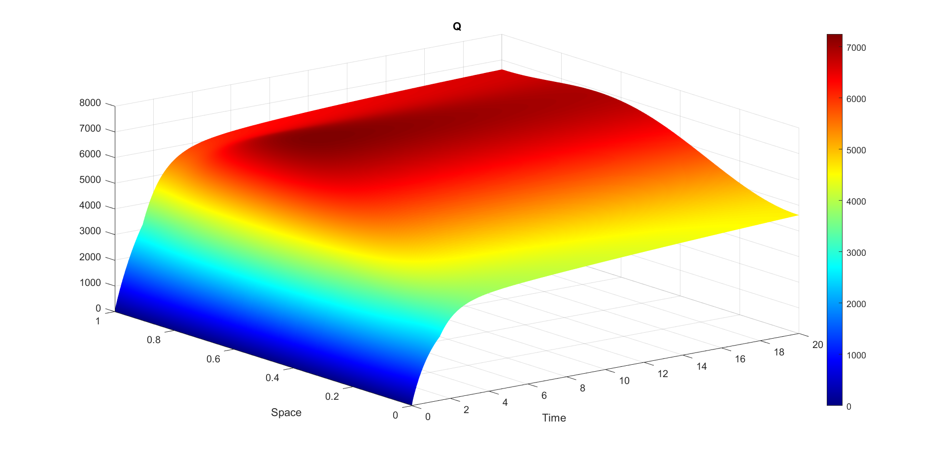
Figure 5: Changes in the quarantined Group in the Presence of Controls.

Figure 8 shows a significant increase in the number of asymptomatic individuals in the absence of control measures. Specifically, the number of asymptomatic cases rises sharply, reaching approximately 3000 persons within the first and second weeks. This substantial increase can be attributed to the lack of intervention, allowing the virus to spread unchecked among the population. The growth in asymptomatic individuals is particularly concerning because these individuals, while not exhibiting symptoms, are still capable of transmitting the virus to others. This hidden spread contributes to a higher number of infected individuals due to the transmission rate $(1-p)\eta$.

\begin{overpic}[width=433.62pt]{Figures/Esans} \put(62.3,34.4){\begin{lx@subfloat@@figure}\begin{minipage}{216.81pt} \includegraphics[width=216.81pt]{Figures/ME} \end{minipage} \@@toccaption{{\lx@tag[ ]{{a}}{}}}\@@caption{{\lx@tag[ ]{{(a)}}{}}}\end{lx@subfloat@@figure} } \end{overpic}

Figure 6: Changes in the Exposed Group Without Control Actions.

\begin{overpic}[width=433.62pt]{Figures/E} \put(62.3,34.4){\begin{lx@subfloat@@figure}\begin{minipage}{216.81pt} \includegraphics[width=216.81pt]{Figures/MEC} \end{minipage} \@@toccaption{{\lx@tag[ ]{{a}}{}}}\@@caption{{\lx@tag[ ]{{(a)}}{}}}\end{lx@subfloat@@figure} } \end{overpic}

Figure 7: Changes in the Exposed Group in the Presence ofControls.

\begin{overpic}[width=433.62pt]{Figures/Asans} \put(62.3,34.4){\begin{lx@subfloat@@figure}\begin{minipage}{216.81pt} \includegraphics[width=216.81pt]{Figures/MA} \end{minipage}\@@toccaption{{\lx@tag[ ]{{a}}{}}}\@@caption{{\lx@tag[ ]{{(a)}}{}}}\end{lx@subfloat@@figure}} \end{overpic}

Figure 8: Changes in the Asymptomatic Group Without Control Actions.

In contrast, when control measures are implemented, as illustrated in Figure 9, the number of asymptomatic individuals is significantly lower, not exceeding 1000 persons. This marked difference underscores the effectiveness of the control strategies in mitigating the spread of the virus. Despite these measures, some increase in asymptomatic cases is still observed, which is natural given that the controls do not directly target this group. The increase in asymptomatic individuals in the presence of controls can also be attributed to the initial pool of exposed individuals transitioning to the asymptomatic category. While the controls effectively reduce the rate at which new individuals become exposed and subsequently asymptomatic, they cannot entirely prevent the existing exposed individuals from progressing through the stages of infection. However, the overall impact is significantly mitigated, demonstrating the critical role of early and effective intervention in controlling the spread of the virus.

\begin{overpic}[width=433.62pt]{Figures/A} \put(62.3,34.4){\begin{lx@subfloat@@figure}\begin{minipage}{216.81pt} \includegraphics[width=216.81pt]{Figures/MAC} \end{minipage} \@@toccaption{{\lx@tag[ ]{{a}}{}}}\@@caption{{\lx@tag[ ]{{(a)}}{}}}\end{lx@subfloat@@figure} } \end{overpic}

Figure 9: Changes in the Asymptomatic Group in the Presence of Controls.

\begin{overpic}[width=433.62pt]{Figures/Isans} \vspace*{2cm} \put(62.3,34.4){\begin{lx@subfloat@@figure}\begin{minipage}{216.81pt} \includegraphics[width=216.81pt]{Figures/MI} \end{minipage} \@@toccaption{{\lx@tag[ ]{{a}}{}}}\@@caption{{\lx@tag[ ]{{(a)}}{}}}\end{lx@subfloat@@figure} } \end{overpic}

Figure 10: Changes in the Infected Group Without Control Actions.

In Figure 10, we observe a substantial increase in the number of infected individuals in the absence of controls, with the infected population rising from 500 to over 2500 cases within approximately 15 days. This rapid escalation is due to the influx from both exposed and asymptomatic groups, significantly contributing to the overall number of active infections. The lack of control measures allows for unchecked transmission, enabling the virus to spread swiftly through the population. As the number of infected individuals grows, the healthcare system becomes increasingly burdened, leading to higher morbidity and mortality rates.

\begin{overpic}[width=433.62pt]{Figures/I} \vspace*{2cm} \put(62.3,34.4){\begin{lx@subfloat@@figure}\begin{minipage}{216.81pt} \includegraphics[width=216.81pt]{Figures/MIC} \end{minipage} \@@toccaption{{\lx@tag[ ]{{a}}{}}}\@@caption{{\lx@tag[ ]{{(a)}}{}}}\end{lx@subfloat@@figure} } \end{overpic}

Figure 11: Changes in the Infected Group in the Presence of Controls.

In contrast, when control measures are implemented, a markedly different trend is observed. As shown in Figure 11, the number of infected individuals starts decreasing from the first day of intervention, reaching zero within 20 days. This rapid reduction underscores the effectiveness of control measures in aiding recovery.

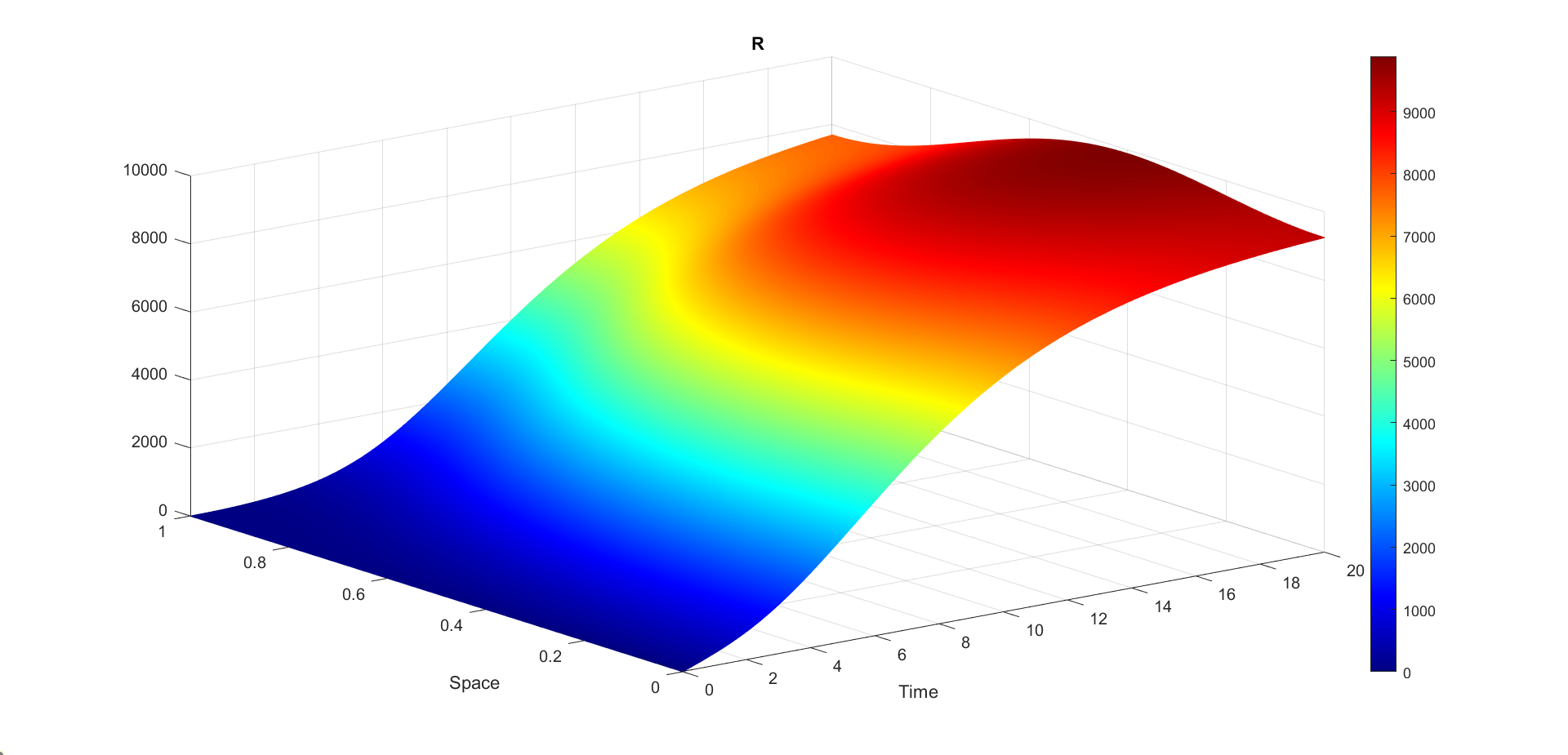
Figure 12: Changes in the Recovered Group Without Control Actions.

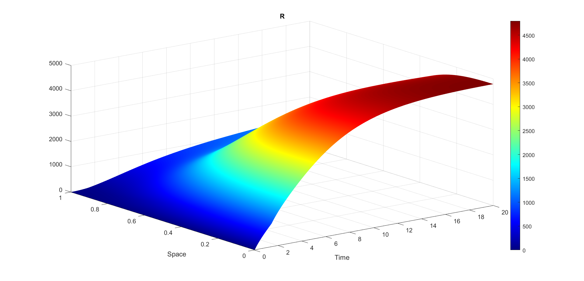
Figure 13: Changes in the Recovered Group in the presence of Controls.

Figure 12 shows the evolution of the recovered population in the absence of control measures. The graph shows a significant number of individuals, more than 9100 people, recovering from the virus. This high number of recoveries suggests that almost the entire population will become infected at some point, as the virus spreads unchecked throughout the community. The large number of recoveries reflects the widespread transmission and eventual resolution of infections without intervention. In contrast, figure 13 shows the effect of control measures on the recovery rate. With controls in place, the number of recoveries does not exceed 3000. This reduction is largely due to the implementation of quarantine measures, which effectively limit the spread of the virus and thus reduce the total number of infections. Figure 5 shows that more than 4300 individuals are quarantined under these measures.

Figure 14: The absolute difference between the total populations of people with and without controls.

Figure 15: The evolution of treatment control function over time.

Figure 16: The evolution of quarantine control function over time.

Figure 14 shows the absolute total population of people with and without control measures. This demonstrates that control measures allow us to save more than 80 people from death due to the infection.

6.1 Discussion and Implications

The analysis of the figures provides valuable insights into the dynamics of the COIVD-19 epidemic under different scenarios. In the absence of control measures, the susceptible population declines rapidly, reaching zero within a week, as illustrated in Figure 2. This results in a significant transition into the exposed category, leading to a surge in asymptomatic and infected cases. The introduction of control measures has a marked effect on the situation. Figure 3 illustrates that the isolation of a proportion of the susceptible population effectively reduces the direct transition to the exposed group, thereby mitigating the overall impact. In the absence of controls, Figure 6 illustrates a marked increase in the number of exposed individuals, reaching a peak of over 2500 within ten days. In contrast, the implementation of control measures (Figure 7) has resulted in a significantly lower peak of exposed individuals, with a maximum of 1000 cases. This indicates the effectiveness of indirect controls in limiting exposure. The growth of asymptomatic individuals is particularly concerning in the absence of control measures, as illustrated in Figure 8, with numbers reaching approximately 3000. This uncontrolled spread poses a significant risk due to asymptomatic transmission. Control measures, as depicted in Figure 9, significantly reduce this number to below 1000, demonstrating their efficacy in curbing the spread, despite the natural progression of existing exposed individuals. Those infected perceive a stark contrast between the two scenarios. In the absence of control measures, Figure 10 illustrates a dramatic increase in the number of infected individuals, reaching over 2500 within 15 days and placing significant strain on healthcare systems. In contrast, the implementation of control measures results in a rapid decrease in infections, reaching zero within 20 days. This highlights the critical role of early intervention in the context of the pandemic. Furthermore, the recovery trends serve to reinforce the impact of the implemented controls. Figure 12 illustrates a high recovery count of approximately 9100 individuals in the absence of controls, which reflects a widespread infection. However, the implementation of control measures, as illustrated in Figure 13, has resulted in a reduction in the number of recoveries to approximately 3000. This is attributed to the decreased infection rates, which have been supported by the quarantining of over 4300 individuals (Figure 5). The figures collectively demonstrate the profound effectiveness of control measures in managing and mitigating the spread of the COIVD-19 epidemic. Consequently, as the number of people who can be quarantined against infection and treated for infection increases, the number of lives saved will also increase.

7 Conclusion

In this paper, we have considered a spatiotemporal SEIAR epidemic model that includes a new group called the quarantined population (Q), referred to as the SQEIAR epidemic model. Our primary objective was to mitigate the spread of the infection by reducing the numbers of exposed, asymptomatic, and infected individuals, while implementing quarantine measures for the susceptible population through the application of optimal control theory. Our strategy employs two distinct control actions: the first involves imposing quarantine measures on susceptible individuals to prevent further spread of the disease; the second focuses on providing treatment to infected individuals to reduce the overall infection rate. The dynamic of our model is described by a partial differential equation (PDE). We have rigorously investigated the mathematical properties of our model, including the existence, boundedness, and positivity of the solutions. Furthermore, we have established the existence of an optimal solution, characterized by an optimal control strategy, by minimizing a specifically defined cost functional. To validate our theoretical findings, we conducted numerical simulations, applying our model to the real-world scenario of the COVID-19 pandemic. These simulations demonstrate the practical viability and effectiveness of our approach, highlighting the potential for significant reductions in infection rates through the implementation of our proposed control strategies.

Disclosure statement

This work is free from any conflicts of interest.

Funding

The authors state that they have no known financial interests or personal relationships that could have influenced the work presented in this paper.

References

• World Health Organization (2020) World Health Organization. (2020). Coronavirus disease 2019 (COVID-19): situation report, 99.
• Abbasi et al. (2020) Abbasi, Z., Zamani, I., Mehra, A. H., et al. (2020). Optimal control design of impulsive SQEIAR epidemic models with application to COVID-19. Chaos, Solitons & Fractals, 139, 110054.
• Aquino et al. (2020) Aquino, E. M., Silveira, I. H., Pescarini, J. M., et al. (2020). Social distancing measures to control the COVID-19 pandemic: potential impacts and challenges in Brazil. Ciencia & saude coletiva, 25, 2423-2446.
• Araz (2021) Araz, S. I. (2021). Analysis of a COVID-19 model: optimal control, stability and simulations. Alexandria Engineering Journal, 60(1), 647-658.
• Asamoah et al. (2022) Asamoah, J. K. K., Okyere, E., Abedimi, A., et al. (2022). Optimal control and comprehensive cost-effectiveness analysis for COVID-19. Results in Physics, 33, 105177.
• Benke et al. (2020) Benke, C., Autenrieth, L. K., Asselmann, E., et al. (2020). Lockdown, quarantine measures, and social distancing: Associations with depression, anxiety and distress at the beginning of the COVID-19 pandemic among adults from Germany. Psychiatry research, 293, 113462.
• Carli et al. (2020) Carli, R., Cavone, G., Epicoco, N., et al. (2020). Model predictive control to mitigate the COVID-19 outbreak in a multi-region scenario. Annual Reviews in Control, 50, 373-393.
• Conti (2008) Conti, A. A. (2008). Quarantine through history. International Encyclopedia of Public Health, 454.
• Davies et al. (2020) Davies, N. G., Klepac, P., Liu, Y., et al. (2020). Age-dependent effects in the transmission and control of COVID-19 epidemics. Nature medicine, 26(8), 1205-1211.
• Diop et al. (2024) DIOP, Mamadou Abdoul, ELGHANDOURI, Mohammed, et EZZINBI, Khalil. Optimal Control of General Impulsive VS-EIAR Epidemic Models with Application to Covid-19. arXiv preprint arXiv:2406.00864, 2024.
• Gensini et al. (2004) Gensini, G. F., Yacoub, M. H., & Conti, A. A. (2004). The concept of quarantine in history: from plague to SARS. Journal of Infection, 49(4), 257-261.
• Guner et al. (2020) Guner, H. R., Hasanglu, I., & Aktas, F. (2020). COVID-19: Prevention and control measures in community. Turkish Journal of medical sciences, 50(9), 571-577.
• Harapan et al. (2020) Harapan, H., Itoh, N., Yufika, A., et al. (2020). Coronavirus disease 2019 (COVID-19): A literature review. Journal of infection and public health, 13(5), 667-673.
• Huremovic (2019) Huremovic, D. (2019). Social distancing, quarantine, and isolation. In Psychiatry of pandemics: a mental health response to infection outbreak (pp. 85-94).
• Kohler et al. (2021) Kohler, J., Schwenkel, L., Koch, A., et al. (2021). Robust and optimal predictive control of the COVID-19 outbreak. Annual Reviews in Control, 51, 525-539.
• Lai et al. (2020) Lai, C., Shih, T. P., Ko, W. C., et al. (2020). Severe acute respiratory syndrome coronavirus 2 (SARS-CoV-2) and coronavirus disease-2019 (COVID-19): The epidemic and the challenges. International journal of antimicrobial agents, 55(3), 105924.
• Li et al. (2020) Li, Q., Guan, X., Wu, P., et al. (2020). Early transmission dynamics in Wuhan, China, of novel coronavirus–infected pneumonia. New England journal of medicine.
• Libotte et al. (2020) Libotte, G. B., Lobato, S. F., Platt, G. M., et al. (2020). Determination of an optimal control strategy for vaccine administration in COVID-19 pandemic treatment. Computer methods and programs in biomedicine, 196, 105664.
• Mackowiak & Sehdev (2002) Mackowiak, P. A., & Sehdev, P. S. (2002). The origin of quarantine. Clinical Infectious Diseases, 35(9), 1071-1072.
• Meng et al. (2020) Meng, L., Hua, F., & Bian, Z. (2020). Coronavirus disease 2019 (COVID-19): emerging and future challenges for dental and oral medicine. Journal of dental research, 99(5), 481-487.
• Moghadas et al. (2020) Moghadas, S. M., Fitzpatrick, M. C., Sah, P., et al. (2020). The implications of silent transmission for the control of COVID-19 outbreaks. Proceedings of the National Academy of Sciences, 117(30), 17513-17515.
• Morato et al. (2020) Morato, M. M., Bastos, S. B., Cajueiro, D. O., et al. (2020). An optimal predictive control strategy for COVID-19 (SARS-CoV-2) social distancing policies in Brazil. Annual reviews in control, 50, 417-431.
• Iwami et al. (2007) Iwami, S., Takeuchi, Y., & Liu, X. (2007). Avian–human influenza epidemic model. Mathematical biosciences, 207(1), 1-25.
• Jiang et al. (2020) Jiang, F., Deng, L., Zhang, L., et al. (2020). Review of the clinical characteristics of coronavirus disease 2019 (COVID-19). Journal of general internal medicine, 35, 1545-1549.
• Jin et al. (2020) Jin, Y., Yang, H., Ji, W., et al. (2020). Virology, epidemiology, pathogenesis, and control of COVID-19. Viruses, 12(4), 372.
• Okyer et al. (2020) Okyer, E., De-Graft Ankamah, J., Hunkpe, A. K., et al. (2020). Deterministic epidemic models for ebola infection with time-dependent controls. Discrete Dynamics in Nature and Society, 2020.
• Pazy (1983) Pazy, A. (1983). Semigroup of Linear Operators and Applications to Partial Equations (Vol. 44). Springer Science and Business Media.
• Pellis et al. (2015) Pellis, L., Ball, F., Bansal, S., et al. (2015). Eight challenges for network epidemic models. Epidemics, 10, 58-62.
• Peni et al. (2020) Peni, T., Csutak, B., Szederkeny, G., et al. (2020). Nonlinear model predictive control with logic constraints for COVID-19 management. Nonlinear Dynamics, 102, 1965
• Rachah et al. (2016) Rachah, A., & Torres, D. F. (2016). Dynamics and optimal control of Ebola transmission. Mathematics in Computer Science, 10(3), 331-342.
• Riou and Althaus (2020) Riou, J., & Althaus, C. L. (2020). Pattern of early human-to-human transmission of Wuhan 2019 novel coronavirus (2019-nCoV), December 2019 to January 2020. Eurosurveillance, 25(4), 2000058.
• Scarabaggio et al. (2021) Scarabaggio, P., Carli, R., Cavone, G., et al. (2021). Nonpharmaceutical stochastic optimal control strategies to mitigate the COVID-19 spread. IEEE Transactions on Automation Science and Engineering, 19(2), 560-575.
• Shen et al. (2021) Shen, Z. H., Chu, Y. M., Khan, M. A., et al. (2021). Mathematical modeling and optimal control of the COVID-19 dynamics. Results in Physics, 31, 105028.
• Sohrabi et al. (2020) Sohrabi, C., Alsafi, Z., O’neill, N., et al. (2020). World Health Organization declares global emergency: A review of the 2019 novel coronavirus (COVID-19). International Journal of Surgery, 76, 71-76.
• Samoilenko and Perestyuk (1995) Samoilenko, A. M., & Perestyuk, N. A. (1995). Impulsive Differential Equations (Vol. 14). World Scientific, Singapore.
• Tang et al. (2020) Tang, B., Xia, F., Tang, S., et al. (2020). The effectiveness of quarantine and isolation determine the trend of the COVID-19 epidemics in the final phase of the current outbreak in China. International Journal of Infectious Diseases, 95, 288-293.