Positive bias makes tensor-network contraction
tractable

Abstract

Tensor network contraction is a powerful computational tool in quantum many-body physics, quantum information and quantum chemistry. The complexity of contracting a tensor network is thought to mainly depend on its entanglement properties, as reflected by the Schmidt rank across bipartite cuts. Here, we study how the complexity of tensor-network contraction depends on a different notion of quantumness, namely, the sign structure of its entries. We tackle this question rigorously by investigating the complexity of contracting tensor networks whose entries have a positive bias.

We show that for intermediate bond dimension $d\gtrsim n$, a small positive mean value $\gtrsim 1/d$ of the tensor entries already dramatically decreases the computational complexity of approximately contracting random tensor networks, enabling a quasi-polynomial time algorithm for arbitrary $1/\mathrm{poly}(n)$ multiplicative approximation. At the same time exactly contracting such tensor networks remains $\#\mbox{\bf P}$-hard, like for the zero-mean case [HHEG20]. The mean value $1/d$ matches the phase transition point observed in [CJHS24]. Our proof makes use of Barvinok’s method for approximate counting and the technique of mapping random instances to statistical mechanical models. We further consider the worst-case complexity of approximate contraction of positive tensor networks, where all entries are non-negative. We first give a simple proof showing that a multiplicative approximation with error exponentially close to one is at least StoqMA-hard. We then show that when considering additive error in the matrix $1$-norm, the contraction of positive tensor network is BPP-complete. This result compares to Arad and Landau’s [AL10] result, which shows that for general tensor networks, approximate contraction up to matrix $2$-norm additive error is BQP-complete.

Our work thus identifies new parameter regimes in terms of the positivity of the tensor entries in which tensor networks can be (nearly) efficiently contracted.

1 Introduction

Tensor network contraction is a powerful computational tool for studying quantum information and quantum many-body systems. It is widely used in estimating ground state properties [Whi93, Whi92, MVC07, VC21], approximating partition functions [EV15, ZXC⁺10], simulating evolution of quantum circuits [MS08, PGN⁺17, HZN⁺20], as well as decoding for quantum error correcting codes [FP14, BSV14]. Mathematically, a tensor network $T\coloneqq T(G,M)$ on a graph $G=(V,E)$ can be interpreted as an edge labeling model. Each edge can be labeled by one of $d$ different colors, where $d$ is called the bond dimension. Each vertex $v$ is associated with a function $M^{[v]}$, called tensor, whose value depends on the labels of edges adjacent to $v$. The tensor $M^{[v]}$ can be represented as a vector by enumerating its values with respect to various edge labeling. For any edge labeling $c$, denote the value (entry) of the tensor $M^{[v]}$ by $M^{[v]}_{c}$. The contraction value of tensor network is defined to be

$$\chi(T)\coloneqq\sum_{\text{edge labeling $c$}\,\,\,}\prod_{v\in V}M^{[v]}_{c}.$$ (1)

In applications of tensor networks, the contraction value represents the quantities of interest and the goal of tensor-network contraction algorithms is to compute the contraction value to high precision.

It is therefore a fundamental question to determine when $\chi(T)$ can be computed efficiently. Despite the practical and foundational importance of this question, unfortunately most rigorous results show that tensor network contraction is extremely hard, with very few tractable cases known, that is, cases for which a (quasi-)polynomial time algorithm exists. Specifically, it is well-known that computing $\chi(T)$ exactly is $\#\mbox{\bf P}$-hard [SWVC07] and therefore intractable in the worst case. The hardness can be further strengthened to the average case, where Haferkamp et al. [HHEG20] showed that even for random tensor networks on a 2D lattice, computing $\chi(T)$ exactly remains $\#\mbox{\bf P}$-hard for typical instances. There, the randomness is modeled by sampling the entries of the tensor network iid. from a Gaussian distribution with zero mean and unit variance. Conversely, (quasi-)polynomial time algorithms are only known for restricted cases, like tensor networks on simple graphs of small tree-width [MS08], for example 1D line or tree; or for restrictive symmetric tensor network [PR17] where each entry is very close to $1$, which requires that $\forall c,v,|M^{[v]}_{c}-1|\leq 0.35/(\Delta+1)$, where $\Delta$ is the maximum degree of the graph. Besides, for tensor networks with uniformly gapped parent Hamiltonians, (quasi)-polynomial time algorithm is known for computing local expectation values [SBE17].

But while efficient and provably correct tensor-network contraction algorithms are rare, for many many-body physics applications, state-of-the-art numerical algorithms achieve desired accuracy in practice [Orú19, Ban23]. To obtain a better understanding of when and why such heuristics work, it is important to identify new tractable cases in tensor network contraction. With this goal in mind, a recent line of work suggests an interesting direction, namely, that the sign structure of the tensor entries influences the entanglement and therefore affects the the complexity of tensor network contraction [GC22, CJHS24]. In particular, it has been observed that there is a sharp phase transition in the entanglement thus the complexity of approximating random tensor networks, when the mean of the entries is shifted from zero to positive [GC22, CJHS24].

1.1 Main results and technical highlights

In this work, we rigorously investigate the impact of sign structure on the complexity of tensor network contraction in various regimes. We mainly focus on the contraction of the physically motivated 2D tensor networks, which are widely used as ground state ansatzes for local Hamiltonians [Cor16, VHCV16] (Projected Entangled Pair States) and for the simulation of quantum circuits [GLX⁺19].

Recall that for random 2D tensor network whose entry has zero mean, the exact contraction is $\#\mbox{\bf P}$-hard [HHEG20]. We first show that a positive bias does not decrease the complexity of the exact contraction:

Theorem 1 (Informal version of Theorem 25).

The exact contraction of random 2D tensor network whose entries are iid. sampled from a Gaussian distribution with positive mean and unit variance remains $\#\mbox{\bf P}$-hard.

While Theorem 1 indicates the exact contraction remains hard, our main result is proving that a small positive mean significantly decreases the computational complexity of multiplicative approximation, enabling a quasi-polynomial time algorithm. This provides rigorous evidence that the sign structure of the tensor entries influences the contraction complexity, as observed and conjectured in previous works [GC22, CJHS24]. In particular, we show that

Theorem 2 (Informal version of Theorem 15).

For random 2D tensor network with intermediate bond dimension $d\gtrsim n$, where the entries are iid.  sampled from Gaussian distribution with mean $\mu\gtrsim 1/d$ and unit variance, there exists a quasi-polynomial time algorithm which with high probability approximates the contraction value up to arbitrary $1/poly$ multiplicative error.

Here $a\gtrsim b$ means that $a$ scales at least as fast as $b$.

While it is expected that tensor network contraction becomes easier when all entries are positive so that there is no sign problem, our result is much more fine-grained than this belief since our tensor network is only slightly positive, that is, a significant portion of the tensor entries are still negative. In particular, note that the mean value $\gtrsim 1/d$ is far less than the unit variance of the tensor entries. Compared to previous work [PR17] which shows that tensor-networks whose all entries are close to $1$ can be contracted using Barvinok’s method, our result allows the entries to have significant fluctuations and to be a mixture of positive and negative values. We also note that the threshold value $\gtrsim 1/d$ matches the phase transition point predicted in [CJHS24] with respect to the entanglement-based contraction algorithm. The fact that two different methods (our algorithm and the entanglement-based algorithm) admit the same threshold might indicate that there is a genuine phase transition in the complexity of tensor network contraction at this point. The requirement of $d\gtrsim n$ on the bond dimension in Theorem 2 is due to the fact that certain concentration effects set in at $d\sim n$. One may wonder then whether the intermediate bond dimension and the nonzero mean make the mean contraction value $\mu^{n}d^{2n}$ (attained when all entries in the tensor network take the mean value $\mu$) a precise guess for the contraction value, that is $\chi(T)=\mu^{n}d^{2n}(1+1/poly(n))$. This is not the case since a simple lower bound shows that the second moment of $\chi(T)/(\mu^{n}d^{2n})$ is at least $2$. In comparison, our algorithm can achieve an arbitrary $1/poly(n)$ multiplicative error in quasi-polynomial runtime; recall Theorem 2. Besides, although Theorem 2 is formulated for random 2D tensor networks, the proposed algorithm is well-defined and runs in quasi-polynomial time for an arbitrary graph $G$ of constant degree, which may inspire new heuristic algorithms for general tensor networks.

Besides studying the average case complexity for approximating slightly positive tensor networks, we also investigate the complexity of approximating (fully) positive tensor networks, where all the entries are positive. Approximate contraction of positive tensor network is directly related to approximate counting, we give a simple proof to show that

Theorem 3 (Informal version of Theorem 31).

$1/poly(n)$ multiplicative approximation of positive tensor network is StoqMA-hard. The StoqMA-hard remains even if we relax the multiplicative error from $1/poly(n)$ to a value exponentially close to one.

Here, StoqMA is the complexity class whose canonical complete problem is to decide the ground energy for stoquastic Hamiltonians [BBT06].

In addition to multiplicative approximation, we also investigate the impact of sign in the hardness of tensor network contraction w.r.t. certain additive error. In particular, previously Arad and Landau [AL10] showed that approximating the contraction value w.r.t. the matrix $2$-norm additive error is equivalent to quantum computation, that is BQP-complete. In contrast, we prove that if the tensor network is positive, where all entries are non-negative, then approximating the contraction value w.r.t matrix $1$-norm additive error is equivalent to classical computation, that is BPP-complete.

Theorem 4 (Informal version of Theorem 27).

Given a positive tensor network $T\coloneqq T(G,M)$ on a constant-degree graph $G$. Given an arbitrary order of the vertex $\{v\}_{v}$, one can view each tensor $M^{[v]}$ as a matrix $O^{[v]}$ by specifying the in-edges and out-edges. It is BPP-complete to estimate $\chi(T)$ with additive error $\epsilon\Delta_{1}$, for $\Delta_{1}\coloneqq\prod_{v}\|O^{[v]}\|_{1}$ and $\epsilon=1/poly(n).$

Technically [AL10] simulates general matrix multiplication by quantum circuits. In Theorem 4 we simulate non-negative matrix multiplication by random walks.

Technical highlights. Our main technical contribution is to show that a small mean value dramatically decreases the complexity of approximate contraction. Our result significantly extends the regime in which efficient approximate contraction algorithms for tensor networks are known. This is formalized and proved in Theorem 2. The algorithm in Theorem 2 differs from commonly used numerical algorithms for tensor network contraction, which are based on the truncation of singular value decomposition and whose performance is determined by entanglement properties [Has07, ALVV17]. Instead, for Theorem 2 we use Barvinok’s method from approximate counting. This method has previously been used for approximating the permanent, the hafnian [Bar16a, Bar16b] and partition functions [Bar14, PR17].

At a high level, Barvinok’s method interprets the contraction value $\chi(T)$ as a polynomial $G(z)$ where $G(1)=\chi(T)$, and uses Taylor expansion of $\ln G(z)$ at $z=0$ to get an additive error approximation of $\ln G(1)$, thus an multiplicative approximation of $\chi(T)$. The key technical part of applying Barvinok’s method to different tasks is proving the corresponding $G(z)$ is root-free in the disk centered at $0$ with radius slightly larger than $1$, which ensures that $\ln G(z)$ is analytic in this disk. Denote this disk as $\mathcal{B}$. Previously Patel and Regts [PR17] had applied Barvinok’s method to symmetric tensor networks where all the entries are close to $1$ within error $0.35/5=0.07$, by proving that $G(z)$ is root-free in $\mathcal{B}$. Our setting allows entries to have significant fluctuations, thus the root-free proof in [PR17] does not apply. We circumvent this problem using the following two ideas:

• Root-free strip inspired from approximating random permanent. Instead of applying Barvinok’s method directly and proving $G(z)$ is root-free in the disk $\mathcal{B}$, we apply a variant of Barvinok’s method used for approximating random permanents by Eldar and Mehraban [EM18]. There, the idea is to use Jensen’s formula to find a root-free strip connecting $0$ and $1$. The advantage of this variant is that it allows for a constant number of zeros in the unit disk $\mathcal{B}$ as long as there is a root-free path of some width connecting $0$ and $1$. We notice that this method from approximating permanent can also be applied to random tensor networks. In particular, using Jensen’s formula [EM18], the number of roots in $\mathcal{B}$ can be bounded by estimating the second moment $E|h(z)|^{2}$, where $h(z)$ is a rescaled version of $G(z)$, and $E$ denotes the expectation value over the randomness of the tensor network. Besides, compared to [EM18], in our setting we use a different and much simpler method to find the root-free strip.

• Mapping random instance to statistical mechanical model. Since we are working on random tensor networks, the technique used by Eldar and Mehraban [EM18] to bound $E|h(z)|^{2}$ for random permanents fails entirely. To bound $E|h(z)|^{2}$ for random tensor networks, we adapt a technique of mapping random instances to a classical statistical mechanical model (statmech model). This technique has been used in the physics literature to study phase transitions in random tensor networks [YLFC22, LC21, HNQ⁺16] and random circuits [BCA20, BBA21].

  Although in general such mapping and the properties of the statmech model like its partition function are hard to analyze, and heuristic approximations are needed in many related literature, we notice that in our application the statmech model is simple enough to obtain a rigorous result. In particular, we show that $E|h(z)|^{2}$ is proportional to the partition function of a 2D Ising model with magnetic field parameterized by $z$. Then we further use the finite-size variant of the Onsager solution of the 2D Ising model [Kau49, Maj66] to get a decent estimate of $E|h(z)|^{2}$ for relevant ranges of $z$, allowing the Barvinok method to be applied.

1.2 Conclusions and open problems

We investigate how the contraction complexity of tensor networks depends on the sign structure of the tensor entries. For random tensor networks in 2D, we show that there is a quasi-polynomial time approximation algorithm if the entries are drawn with a small nonzero mean and intermediate bond dimension. At the same time, exactly computing the contraction value in this setting remains $\#\mbox{\bf P}$-hard. Our work thus provides rigorous evidence for the observations [GC22, CJHS24] that shifting the mean by a small amount away from zero dramatically decreases the contraction complexity. Compared to [PR17] which similarly uses Barvinok method but requires all entries to be close to $1$, our setting allows significant fluctuations in the entries and greatly extends the known region where (quasi-)polynomial time average-case contraction algorithms exist. While it is expected that tensor network contraction becomes easier when all entries are positive, our result suggests that even for slightly positive tensor networks, one can still utilize the sign structure to obtain a (quasi-)efficient algorithm. Moreover, [CJHS24] observed that the standard entanglement-based contraction algorithm starts working at $\mu\gtrsim 1/d$. We show that a completely different rigorous Barvinok-based algorithm also starts working at $\mu\gtrsim 1/d$. This might indicate that there is a genuine phase transition in the complexity of tensor-network contraction happening here.

Indeed, we also assess the worst-case complexity of approximating fully positive tensor networks. Specifically, we prove that approximating the contraction value of positive tensor networks multiplicative error close to unity is StoqMA-hard. But when requiring only an inverse polynomial additive error in matrix $1$-norm there exists an efficient classical algorithm.

Our work initiates the rigorous study of how the computational difficulty of contracting tensor networks depends on the sign structure of the tensor entries. If one views the hardness of contraction as a function of mean value and bond dimension, while we identify a new tractable region, there are many open questions left.

• First, while our approximation algorithm based on Barvinok’s method works for typical instances, it remains an open question to what extent a positive bias can ease practical tensor network contraction. It would therefore be interesting to understand whether our algorithm or variations of it can aid in practically interesting cases.

• Moreover, our current proof works for intermediate bond dimension but not for constant bond dimension. Potentially, techniques like cluster expansion [MH21, HPR19] may be used to design new contraction algorithm for constant bond dimension, proving a correspondent of Theorem 4 for that setting. It might be worth mentioning that a direct application of cluster expansion does not work, where one can prove the expansion series is not absolutely convergent. More refined techniques are thus required.

• Finally, although current numerical algorithms have poor performance for zero-mean tensor network contraction, there is no known rigorous complexity result to establish the hardness of approximate contraction.

In the context of approximating fully positive tensor networks, it would be interesting to see whether there exists an efficient classical algorithm that can achieve the same ($2$-norm) precision as a quantum computer for positive tensor networks, or whether there is a room for quantum advantage even for positive tensor networks.

1.3 Structure of the manuscript

The structure of this manuscript is as follows. In Section 2 we define notations and tensor networks. In Section 3 we review Barvinok’s method and its variant. In section 4 we adapt Barvinok’s method to tensor network contraction. In Section 5 we give a quasi-polynomial time algorithm for approximating random 2D tensor networks with small mean and intermediate bond dimension. In Section 6 we prove the results concerning approximating positive tensor networks.

2 Notation and tensor networks

In this section, we introduce necessary notations and definitions for tensor networks.

Notation. We use $[k]$ for $\{0,1,\ldots,k-1\}$. We use $\overline{z}$ to denote its complex conjugate. For $v\in\mathbb{C}$ and $\epsilon\in\mathbb{R}$, we say $\hat{v}$ approximates $v$ with $\epsilon$-multiplicative error if $|v-\hat{v}|\leq\epsilon|v|$. For $x\in\{\pm 1\}^{n}$, we use $|x|$ to denote the number of $-1$ in $x$. We use $\delta_{ij}$ for the delta function, where $\delta_{ij}=1$ if $i=j$ and equals $0$ otherwise.

For a matrix $A\in\mathbb{C}^{s\times t}$, the matrix $p$-norm is defined as

$$\|A\|_{p}\coloneqq\sup_{x\neq 0,x\in\mathbb{R}^{t}}\frac{\|Ax\|_{p}}{\|x\|_{p}}$$ (2)

The $2$-norm $\|A\|_{2}$ is known as the spectral norm. The $1$-norm equals to the maximum of the absolute column sum, that is

$$\|A\|_{1}=\max_{1\leq j\leq t}\sum_{i=1}^{s}|A_{ij}|.$$

For $\mu,\sigma\in\mathbb{R}$, we use $X\sim\mathcal{N}_{\mathbb{R}}(\mu,\sigma^{2})$ to denote that the random variable $X$ is sampled from the Gaussian distribution with mean $\mu$ and standard derivation $\sigma$. For $\mu\in\mathbb{C}$, we use $\Re(\mu),\Im(\mu)\in\mathbb{R}$ to denote the real and imaginary part of $\mu$, i.e. $\mu=\Re(\mu)+\Im(\mu)i$. We use $X\sim\mathcal{N}_{\mathbb{C}}\left(\mu,\sigma^{2}\right)$ if

$$\Re\left(X\right)\sim\mathcal{N}_{\mathbb{R}}\left(\Re(\mu),\frac{\sigma}{2}^{2}\right),\Im(X)\sim\mathcal{N}_{\mathbb{R}}\left(\Im(\mu),\frac{\sigma}{2}^{2}\right).$$

Tensors and tensor networks. A tensor $N$ of rank $k$ and bond dimension $d$ is an array of $d^{k}$ complex numbers which is indexed by $N_{i_{1},i_{2},\ldots,i_{k}}$, where $i_{s}$ takes values from $[d]$ for $1\leq s\leq k$. We call the complex numbers in the array the entries of the tensor $N$. We use $\overline{N}$ to denote the tensor obtained by complex conjugating every entry of $N$. For two tensors $N$ and $M$ with the same rank and bond dimension, the addition $N+M$ is a new tensor obtained by addition of the two arrays. For convenience, in the rest of the paper we assume that all the indices have the same dimension $d$. We will always assume $d=O(poly(n))$.

A tensor network $T\coloneqq T(G,M)$ is described by an $n$-vertex graph $G=(V,E)$ and a set of tensors on vertices, denoted as $M=\{M^{[v]}\}_{v}$. More specifically, on each vertex $v$ of degree $k_{v}$ there is a tensor $M^{[v]}$ of rank $k_{v}$, where the indices $i_{1},\ldots,i_{k_{v}}$ correspond to $k_{v}$ edges. One can interpret $[d]$ as $d$ different colors, and $i_{s}\in[d]$ represents that we label the corresponding edge with color $i_{s}$. Denote this edge labeling as $c:E\rightarrow[d]^{|E|}$, we write $M^{[v]}_{c}\coloneqq M^{[v]}_{i_{1},\ldots,i_{k_{v}}}.$ With an arbitrary ordering of edges, we can conceive of the labeling $c$ as a vector $c\in[d]^{|E|}$. The contraction value of tensor network is then defined to be

$$\chi(T)\coloneqq\sum_{c\in[d]^{|E|}}\prod_{v\in V}M^{[v]}_{c}.$$ (3)

Product and contraction. Besides Eq. (3), another equivalent way of defining the contraction value of tensor network $\chi(T)$ is via a graphical representation, which is more intuitive and will be used in the proofs. As in Figure 1 (a), for a tensor of rank $k$, we represent it as a vertex with $k$ edges. We term such edges which connect to only one vertex free edges.

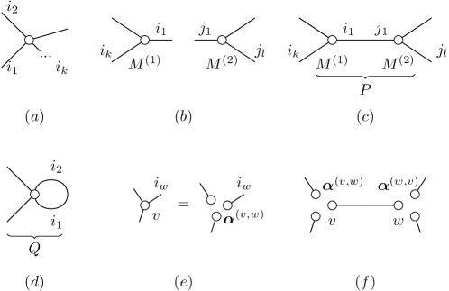
Figure 1: Tensor and operations on tensors. (a) A rank-$k$ tensor. (b) The product of a rank-$k$ and a rank-$l$ tensor. (c) Contracting two tensors by identifying edges $i_{1}$ and $j_{1}$. (d) Contracting two free edges in the same tensor. (e) A special tensor which can be factorized into a product of rank-$1$ tensors. (f) If all tensors have a factorized structure, then the contraction value of tensor network can be computed by contracting the rank-$1$ tensors.

With this graphical representation, we introduce two operations on tensors. Consider a tensor $M^{(1)}$ of rank $k$, with free edges indexed by $i_{1},\ldots,i_{k}$, and another tensor $M^{(2)}$ of rank $l$, with free edges indexed by $j_{1},\ldots,j_{l}$. We use Figure 1 (b) to represent the product of $M^{(1)},M^{(2)}$, that is a new tensor $M^{(1)}\otimes M^{(2)}$ of rank $k+l$ and with free edges indexed by $i_{1},\ldots,i_{k};j_{1},\ldots,j_{l}$, where

$$\left(M^{(1)}\otimes M^{(2)}\right)_{i_{1},\ldots,i_{k},j_{1},\ldots,j_{l}}\coloneqq M^{(1)}_{i_{1},\ldots,i_{k}}M^{(2)}_{j_{1},\ldots,j_{l}}.$$ (4)

The product operation can be generalized to multiple tensors recursively,

$$M^{(1)}\otimes M^{(2)}\otimes M^{(3)}\otimes M^{(4)}\ldots\coloneqq\left(\left(\left(M^{(1)}\otimes M^{(2)}\right)\otimes M^{(3)}\right)\otimes M^{(4)}\right)\ldots$$ (5)

One can check that the order of this recursion does not change the final tensor.

Another operation which defines a new tensor is contraction, that is, connecting different tensors by identifying a free edge of one tensor with a free edge of another tensor and summing over that index. Starting from the two tensors $M^{(1)}$ and $M^{(2)}$, contracting the indices $i_{1}$ and $j_{1}$ results in a new tensor $P$ of rank $k+l-2$, with free edges indexed by $i_{2},\ldots,i_{k},j_{2},\ldots,j_{l}$, where

$$P_{i_{2},\ldots,i_{k},j_{2},\ldots,j_{l}}=\sum_{f\in[d]}M^{(1)}_{f,i_{2},\ldots,i_{k}}M^{(2)}_{f,j_{2},\ldots,j_{l}}.$$ (6)

Graphically, this operation is represented by joining the two contracted edges, see Figure 1 (c).

One can also contract two free edges in the same tensor. Consider the contraction of the indices $i_{1},i_{2}$ of $M^{(1)}$. Figure 1 (d) represents a new tensor $Q$ of rank $k-2$ and with free edges $i_{3},\ldots,i_{k}$ where

$$Q_{i_{3},\ldots,i_{k}}=\sum_{s\in[d]}M^{(1)}_{s,s,i_{3},\ldots,i_{k}}.$$ (7)

The contraction operations can be generalized to contracting multiple pairs of edges by contracting the pairs one by one. Note that the order of contraction does not change the final tensor.

One can check that given a tensor network $T=T(G,M)$, the contraction value of tensor network defined by Eq. (3) is equal to the value obtained when contracting $\bigotimes_{v}M^{[v]}$ by identifying the free edges according to the edges of $G$.

For any vertex $v$, use $N(v)$ for the vertices adjacent to $v$ in $G$.

Example 5.

Here we give an example of how the graphical representation simplifies the computation of the contraction value. Consider a case in which each $M^{[v]}$ has a factorized structure, that is, there exist vectors $\bm{\alpha}^{(v,w)}\in\mathbb{C}^{d}$ for $w\in N(v)$ such that

$$M^{[v]}=\bigotimes_{w\in N(v)}\bm{\alpha}^{(v,w)},$$

equivalently the entry

$$M^{[v]}_{\ldots,i_{w},\ldots}=\prod_{w\in N(v)}\bm{\alpha}^{(v,w)}_{i_{w}}.$$

Then $M^{[v]}$ can be represented by a product of $|N(v)|$ tensors as shown in Figure 1 (e). As a consequence, one can check that in this special case computing $\chi(T)$ is easy: as in Figure 1 (f), one can write $\chi(T)$ in a factorized way, where each edge $(v,w)$ contributes a factor $\langle\bm{\alpha}^{(v,w)},\bm{\alpha}^{(w,v)}\rangle\coloneqq\sum_{f\in[d]}\bm{\alpha}^{(v,w)}_{f}\bm{\alpha}^{(w,v)}_{f}$ as follows:

$$\chi(T) =\sum_{\text{all edge labeling $c$}}\prod_{v}M^{[v]}_{c}$$ (8)

$$=\prod_{\text{edges $(v,w)$}}\langle\bm{\alpha}^{(v,w)},\bm{\alpha}^{(w,v)}\rangle.$$ (9)

2D tensor network. We call a tensor network $T=T(G,M)$ a 2D tensor network if the graph $G$ is a 2D lattice. We assume the lattice has size $L_{1}\times L_{2}$ with $n=L_{1}\times L_{2}$, and satisfies periodic boundary conditions, that is can be mapped onto a torus. The periodic boundary condition is mainly to ease the analysis. In particular, every vertex has degree $4$. For simplicity, we assume that $L_{2}$ is even.

• For $\mu>0$, we define a 2D $(\mu,n,d)$-Gaussian tensor network $T(G,M)$ as an $n$-vertex 2D tensor network with bond dimension $d$, where the entries of every tensor $M^{[v]}$ are iid. sampled from the complex Gaussian distribution $\mathcal{N}_{\mathbb{C}}(\mu,1)$, i.e.

  $$(M^{[v]})_{i_{1},i_{2},i_{3},i_{4}}\stackrel{{\scriptstyle i.i.d.}}{{\sim}}\mathcal{N}_{\mathbb{C}}(\mu,1).$$ (10)

• For technical reasons, for $z\in\mathbb{C}$ we also define the 2D $(z,n,d)$-shifted-Gaussian tensor network $T(G,M)$, which is an $n$-vertex 2D tensor network with bond dimension $d$: For every vertex $v$, Let $(A^{[v]})_{i_{1},i_{2},i_{3},i_{4}}\stackrel{{\scriptstyle i.i.d.}}{{\sim}}\mathcal{N}_{\mathbb{C}}(0,1)$, the entries of $M^{[v]}$ are defined to be

  $$(M^{[v]})_{i_{1},i_{2},i_{3},i_{4}}\coloneqq 1+z\cdot(A^{[v]})_{i_{1},i_{2},i_{3},i_{4}}.$$ (11)

  We write the tensor $M^{[v]}$ as

  $$M^{[v]}=J^{[v]}+zA^{[v]}$$ (12)

  where $J^{[v]}$ is a tensor whose entries are all $1$. Note that $J^{[v]}$ has a factorized structure

  $$J^{[v]}=[1,\ldots,1]^{\otimes 4}.$$

  We abbreviate the 2D $(z,n,d)$-shifted-Gaussian tensor network $T(G,M)$ as $T_{A}(z)$ where $A\coloneqq\{A^{[v]}\}_{v}$.

3 Barvinok’s method and its variant

In this section we review Barvinok’s method, which was first developed by Barvinok [Bar16a, Bar16b], and is a general method for approximate counting. It has been applied to approximating permanents [EM18], hafnians [Bar16a, Bar16b] and partition functions [Bar14, PR17]. In particular, Barvinok’s method was applied to contracting symmetric tensor networks where all entries are very close to $1$ [PR17]. Our setting allows the entries having significant fluctuations where the standard Barvinok’s method fails. Instead our algorithm builds from a special variant of Barvinok’s method used in approximating random permanents [EM18], which we summarize below. All Lemmas and Theorems quoted here are proven in [Bar16a, Bar16b, EM18].

Roughly speaking, the idea of Barvinok’s method is to approximate an analytic function via its Taylor series around $0$. The performance of this approximation depends on the location of the roots of the analytic function.

Consider a polynomial $G(z)$ of degree $n$, where $G(z)\neq 0$ for $z$ on a simply connected open area containing $0$ in the complex plain. We choose the branch of the complex logarithm, denoted as ${\rm{\ln}}\,$, such that ${\rm{\ln}}\,G(0)$ is real. Define $F(z):={\rm{\ln}}\,G(z)$. In our application, $G(1)$ will encode the contraction value of tensor network. An additive approximation of $F(1)$ will give a multiplicative approximation to $G(1)$. For $r,w>0$, we use $\mathcal{B}(r)\subset\mathbb{C}$ to denote the the disk of radius $r$ centered at $0$, and use $\mathcal{T}(re^{i\theta},w)$ to denote the strip of width $w$ around the line between $0$ and $re^{i\theta}$, that is

$$\mathcal{B}(r)\coloneqq\{z\in\mathbb{C}\,\,\big{|}\,\,|z|\leq r\},$$

$$\mathcal{T}(re^{i\theta},w)\coloneqq\{z\in\mathbb{C}\,\,\big{|}\,\,-w\leq\Re(ze^{-i\theta})\leq r+w,\quad|\Im(ze^{-i\theta})|\leq w\}.$$

The following lemma quantifies the approximation error incurred by approximating $F(z)$ using a root-free disk of $G(z)$.

Lemma 6 (Approximation using a root-free disk, see the proof of Lemma 1.2 in [Bar16b]).

Let $G(z)$ be a polynomial of degree $n$ and suppose $G(z)\neq 0$ for all $|z|\leq\eta$ where $\eta>1$. Let $F(z)\coloneqq{\rm{\ln}}\,G(z).$ Then $F(z)$ is analytic for $|z|\leq 1$. Moreover, consider a degree $m$ Taylor approximation of $F(z)$,

$$P_{m}(z)\coloneqq F(0)+\sum_{k=1}^{m}\frac{\partial^{k}F(z)}{\partial z^{k}}\bigg{|}_{z=0}\frac{z^{k}}{k!}$$ (13)

Then, for all $|z|\leq 1$,

$$|F(z)-P_{m}(z)| \leq\frac{n}{(m+1)\eta^{m}(\eta-1)}.$$ (14)

Recall that additive approximation of $F(z)$ implies multiplicative approximation of $G(z)$. To translate Lemma 6 into an efficient algorithm, one further needs to efficiently compute the first few derivatives of $F$. Barvinok shows that the derivatives of $F$ can be efficiently computed using the derivatives of $G$.

Lemma 7 ([Bar16a]).

Let $G(z)$ be a polynomial of degree $n$ and $G(z)\neq 0$. If one can compute the first $l$ derivatives of $G(z)$ at $z=0$ in time $t(n)$, then one can compute the first $l$ derivatives of $F(z)\coloneqq{\rm{\ln}}\,G(z)$ at $z=0$ in time $O(l^{2}t(n))$.

Lemma 6 implies that the Taylor series at $z=0$ gives a good approximation to $F(z)={\rm{\ln}}\,G(z)$, as long as $G(z)$ is root-free in a disk centered at $0$ that contains $z$. Lemma 6 can be generalized to the case in which $G(z)$ is allowed to have roots in the disk, but instead there exists a root-free strip from $0$ to $z$. The main idea in this generalization is to construct a new polynomial $\phi(z)$ which embeds the disk into a strip. Given such $\phi$, we can then approximate $G(\phi(z))$ using the approximation via a root-free disk, since $G(\phi(z))$ is guaranteed to be root free in a disk of some radius. Furthermore, we can still use this approximation to estimate $G(1)$, which will encode our quantity of interest.

Lemma 8 (Embedding a disk into a strip, Lemma 8.1 in [Bar16a]).

For $0<\rho<1$, define

$$\alpha=\alpha(\rho)=1-e^{-\frac{1}{\rho}},\quad\eta=\eta(\rho)=\frac{1-e^{-1-\frac{1}{\rho}}}{1-e^{-\frac{1}{\rho}}}>1,$$ (15)

$$K=K(\rho)=\left\lfloor\left(1+\frac{1}{\rho}\right)e^{1+\frac{1}{\rho}}\right\rfloor\geq 14,\quad\sigma=\sigma(\rho)=\sum_{k=1}^{K}\frac{\alpha^{k}}{k}\text{ and }$$ (16)

$$\phi(z)=\phi_{\rho}(z)=\frac{1}{\sigma}\sum_{k=1}^{K}\frac{(\alpha z)^{k}}{k}.$$ (17)

Then $\phi(z)$ is a polynomial of degree $K$ such that $\phi(0)=0,\phi(1)=1$, and embeds the disk of radius $\eta$ into the strip of width $2\rho$, i.e.,

$$-\rho\leq\Re(\phi(z))\leq 1+2\rho\text{ and }|\Im(\phi(z))|\leq 2\rho\text{ provided }|z|\leq\eta.$$ (18)

Corollary 9 (Approximation using a root-free strip).

Let $G(z)$ be a polynomial of degree $n$ and suppose there exists a constant $\rho\in(0,1)$ such that $G(z)\neq 0$ for all $z$ in the strip $\mathcal{T}(1,2\rho)$. Define $\eta,K,\phi(z)$ as in Lemma 8 where $\eta>1$. Let

$$F(z)\coloneqq{\rm{\ln}}\,G(\phi(z)).$$

Then $F(z)$ is analytic for $|z|\leq 1$. Moreover, consider a degree $m$ Taylor approximation of $F(z)$,

$$P_{m}(z)\coloneqq F(0)+\sum_{k=1}^{m}\frac{\partial^{k}F(z)}{\partial z^{k}}|_{z=0}\frac{z^{k}}{k!}$$ (19)

Then, for all $|z|\leq 1$,

$$|F(z)-P_{m}(z)| \leq\frac{nK}{(m+1)\eta^{m}(\eta-1)}.$$ (20)

Proof.

Recall that $\eta>1$. By Lemma 8 and the assumption that $G(z)\neq 0$ for all $z$ in $\mathcal{T}(1,2\rho)$, we have for any $|z|\leq\eta$, $G(\phi(z))\neq 0$. Note that $G(\phi(z))$ is a polynomial in $z$ of degree $nK$. Then use Lemma 6 w.r.t $G(\phi(z))$ and $F(z)\coloneqq{\rm{\ln}}\,G(\phi(z))$ we prove the Corollary. ∎

In the above Lemmas, we have assumed $G(z)$ is a fixed polynomial, and the performance of the Taylor expansion of $F(z)$ depends on the location of roots of $G(z)$. When $G_{A}(z)$ are random polynomials indexed by randomness $A$, [EM18] illustrates a way of using Jensen’s formula to estimate the expectation of the number of roots.

For convenience of later usage, in the following we use the notation $h_{A}(z)$ for polynomials instead of $G_{A}(z)$. In later applications $h_{A}(z)$ will be a rescaled version of $G_{A}(z)$. By Lemma 11 [EM18] connects the expected number of roots in a disk to the second moment of $h_{A}$.

Definition 10 (Average Sensitivity [EM18]).

Let $h_{A}(z)$ be a random polynomial where $A$ is sampled from some random ensembles and $h_{A}(0)\neq 0$. For any real number $r>0$, the stability of $h_{A}(z)$ at point $r$ is defined as

$$k_{h}(r)\coloneqq E_{\theta}E_{A}\left[\frac{|h_{A}(re^{i\theta})|^{2}}{|h_{A}(0)|^{2}}\right]$$ (21)

where $E_{\theta}[\cdot]=\int_{\theta=0}^{2\pi}[\cdot]\frac{d\theta}{2\pi}$ is the expectation over $\theta$ from a uniform distribution over $[0,2\pi)$, and $E_{A}$ is the expectation over the randomness of $A$.

Lemma 11 (Proposition 8 [EM18]).

Let $h_{A}(z)$ be a random polynomial where $A$ is sampled from some random ensemble and $h_{A}(0)\neq 0$. Let $N_{A}(r)$ be the number of roots of $h_{A}(z)$ inside $\mathcal{B}(r)$, and $0<\lambda<1/2$. Then,

$$E_{A}\left[N_{A}(r-r\lambda)\right]\leq\frac{1}{2\lambda}\ln k_{h}(r).$$ (22)

Lemma 11 bounds the expectation value of the number of roots in $\mathcal{B}(r)$. In later sections, we will apply Lemma 11 to show that our polynomial of interest has very few roots in the disk. This will allow us to find a root-free strip with high probability. For completeness, we provide a proof of Lemma 11 in Appendix B.

4 Tensor network contraction algorithm from Barvinok’s method

We are now ready to present our algorithm for approximate tensor network contraction. The algorithm is based on Barvinok’s method and takes the following inputs

• A tensor network $T=T(G,M)$, where $G=(V,E)$ is a graph comprising $n=|V|$ vertices and has constant degree $\kappa$.

• A precision parameter $\epsilon\in(0,1]$.

The goal is to approximate $\chi(T)$ with $\epsilon$-multiplicative error. In order to achieve this, we will choose the following parameters that will enter the algorithm appropriately.

• A set of non-zero complex values $\{\mu_{v}\}_{v\in G}$. We will choose $\mu_{v}$ to be the mean value of the entries of the tensor $M^{[v]}$ at vertex $v\in V$.

• A complex value $z_{end}\neq 0$.

• A real value $0<\rho<1$. This value will determine the width of the strip $\mathcal{T}(1,2\rho)$ in the complex plane.

The algorithm we describe in this section is well-defined for an arbitrary tensor network. In Section 5 we will apply this algorithm to random 2D tensor network whose entries have a small positive bias and show that it succeeds with high probability.

4.1 The polynomial

To apply Barvinok’s method in Corollary 9, we map the contraction value of tensor network to a polynomial as follows. For each vertex $v$, with some abuse of notations, we use $J^{[v]}$ to represent the tensor by substituting all entries in $M^{[v]}$ by $1$. We define

$$A^{[v]}\coloneqq(\mu_{v}^{-1}M^{[v]}-J^{[v]})\cdot z_{end}^{-1}$$ (23)

In other word,

$$\mu_{v}^{-1}M^{[v]} =J^{[v]}+z_{end}\cdot A^{[v]}$$ (24)

Eq. (24) states that we intepret the normalized version of $M^{[v]}$ as the all-one tensor $J^{[v]}$ interpolated by $A^{[v]}$. We note that we allow $z_{end}$ to be much larger than $1$.

Since the contraction value of $T(G,\{M^{[v]}\}_{v})$ equals $\prod_{v}\mu_{v}$ times the contraction value of the normalized tensor network $T(G,\{\mu_{v}^{-1}M^{[v]}\}_{v})$, without loss of generality, from now on we assume that the tensor network has been normalized and

$$M^{[v]} =J^{[v]}+z_{end}\cdot A^{[v]}$$ (25)

If we substitute $z_{end}$ with a variable $z$ in Eq. (25) for each tensor $M^{[v]}$, we will obtain a family of new tensor networks, denoted by $T_{A}(z)$. The contraction value $\chi(T_{A}(z))$ is a degree-$n$ polynomial in $z$. Denoting this polynomial as $g_{A}(z)$, we have

$$g_{A}(z)=\chi(T_{A}(z)),\quad 0\leq z\leq z_{end}$$ (26)

$$g_{A}(z_{end})=\chi(T_{A}(z_{end}))=\chi(T).$$ (27)

Recall that $0<\rho<1$. Define the polynomial $\phi(z)$ as in Lemma 8. For convenience of applying Barvinok’s method, we also define $G_{A}(z)$ by rescaling $g(z)$,

$$G_{A}(z)\coloneqq g_{A}(z\cdot z_{end}),\quad 0\leq z\leq 1.$$ (28)

$$F_{A}(z)\coloneqq{\rm{\ln}}\,G_{A}(\phi(z)).$$ (29)

$F_{A}(z)$ will be analytic in the disk $\mathcal{B}(1)$ if $G_{A}(z)$ is root-free in the strip $\mathcal{T}(1,2\rho)$.

4.2 Computing the derivatives of $g_{A}$

We first note that the first few derivatives of $g_{A}(z)$ can be computed efficiently.

Lemma 12.

For any integer $m$, the first $m$ derivatives $\{g_{A}^{(k)}(0)\}_{k=0,\ldots,m}$ can be computed in time $O(m^{2}d^{\kappa m}n^{m+1})$.

Proof.

For any subset $S\subseteq V$, we denote by $\frac{\partial T_{A}(z)}{\partial S}$ the tensor network which is obtained by substituting the tensor $M^{[v]}$ with $A^{[v]}$ at every vertex $v\in S$. Using the product rule of derivatives and induction on $k$, one can check that

$$\frac{\partial^{k}g_{A}(z)}{\partial z^{k}}=\sum_{S\subseteq V,|S|=k}\chi\left(\frac{\partial T_{A}(z)}{\partial S}\right)\cdot k!$$ (30)

In particular, note that when $z=0$, by the definition of $\frac{\partial T_{A}(0)}{\partial S}$, for any vertex $w\not\in S$, the corresponding tensor at $w$ in $\frac{\partial T_{A}(0)}{\partial S}$ is

$$M^{[v]}=J^{[v]}+0\cdot A^{[v]}=J^{[v]}.$$

As in Example 5 and Figure 1 (f), we can decompose each tensor $J^{[v]}=[1,\ldots,1]^{\otimes\kappa}$ as a product of $\kappa$ all-one vectors $[1,\ldots,1]$. Then the graphical representation of $\frac{\partial T_{A}(0)}{\partial S}$ consists of many disconnected sub-graphs, where each sub-graph has at most $|S|\leq m$ vertices. The contraction value $\chi(\frac{\partial T_{A}(0)}{\partial S})$ is the product of the contraction value of each subgraph, and can be computed in time $n\cdot O(d^{\kappa m}m)$. Here $n$ is an upper bound of the number of sub-graphs, and $O(d^{\kappa m}m)$ is the cost of directly contracting an $m$ vertices subgraph of a tensor network on degree-$\kappa$ graph. Thus by Eq. (30) for any $k\leq m$, $g^{(k)}_{A}(0)$ can be computed in time $O(n^{m}d^{\kappa m}nm)$. We conclude that the first $m$ derivatives $\{g^{(k)}(0)\}_{k=0,\ldots,m}$ can be computed in time $O(m^{2}d^{\kappa m}n^{m+1})$. ∎

In later proofs we will set $m=O\left(\ln\left(n/\epsilon\right)\right)$. When $d=poly(n)$ and $\epsilon=O(1/poly(n))$, the cost $O(m^{2}d^{4m}n^{m+1})$ of computing the $m$-th derivative is then quasi-polynomial.

Using Lemma 12 one can efficiently compute the first few derivatives of $F_{A}(z)$.

Lemma 13.

Assume that $\rho$ is a constant. Then for any integer $m$, the first $m$ derivatives of $\{F^{(k)}_{A}(0)\}_{k=1}^{m}$ can be computed in time

$$O\left(m^{4}d^{\kappa m}n^{m+1}+m^{6}\right).$$

Proof.

By Lemma 12 and the definition of $G_{A}(z)$, the first $m$ derivatives $\{G_{A}^{(k)}(0)\}_{k=0}^{m}$ can be computed in time $O(m^{2}d^{\kappa m}n^{m+1})$. Besides, from Lemma 8 and the assumption that $\rho$ in the definition of $\phi$ is a constant, $\phi(z)$ is a polynomial of degree $K$ where $K=K(\rho)$ is a constant, thus the first $m$ derivatives $\{\phi^{(k)}(0)\}_{k=0}^{m}$ can be computed in time $O(m)$. Thus by Lemma 35 in Appendix B, one can compute the the first $m$ derivatives of the composite function $G_{A}(\phi(z))$ at $z=0$ in time

$$O(m^{2}d^{\kappa m}n^{m+1}+m^{4}).$$

Note that $K$ is a constant and $G_{A}(\phi(z))$ is a polynomial of degree $nK$. Then by Lemma 7, we can compute the first $m$ derivatives $F_{A}^{(k)}(0)$ in time

$$O\left(m^{4}d^{\kappa m}n^{m+1}+m^{6}\right).$$

∎

4.3 The algorithm and its performance

Our goal is to approximate ${\rm{\ln}}\,G_{A}(1)={\rm{\ln}}\,G_{A}(\phi(1))$ with respect to an additive error, which will give a multiplicative approximation to $G_{A}(1)=\chi(T)$. The algorithm is just computing the derivatives and $P_{m}(z)$ in Corollary 9, that is Algorithm 1.

Algorithm 1 Barvinok($G_{A},m,\rho$)

1:Let $F_{A}(z)\coloneqq\ln G_{A}(\phi(z))$ with $\phi=\phi_{\rho}$ as defined in Eq. (17).

2:Compute the first $m$ derivatives $\{F^{(k)}_{A}(0)\}_{k=0}^{m}$ of $F_{A}$ using Lemma 13.

3:Compute $P_{m}(1)\coloneqq F(0)+\sum_{k=1}^{m}F^{(k)}_{A}(0)\frac{1}{k!}$ .

4:Return $\hat{\chi}(T):=e^{P_{m}(1)}$.

Algorithm 1 returns a good approximation of $\chi(T)$ with multiplicative error $\epsilon$ if $G_{A}(z)$ is root-free in $\mathcal{T}(1,2\rho)$ and we set $m=O(\ln(n/\epsilon))$.

Theorem 14.

Let $0<\rho<1$ be a constant. If $G_{A}(z)\neq 0$ for any $z$ in strip $\mathcal{T}(1,2\rho)$, then for any $\epsilon$, Algorithm 1 runs in time

$$O\left(m^{4}d^{\kappa m}n^{m+1}+m^{6}\right).$$

Choosing $m=O(\ln(n/\epsilon))$, Algorithm 1 outputs a value $\hat{\chi}(T)$ that approximates $\chi(T)$ with $\epsilon$-multiplicative error. That is

$$|\hat{\chi}(T)-\chi(T)|\leq\epsilon|\chi(T)|.$$

Proof.

As in Corollary 9 and Lemma 8, we define two constants $\eta,K$ from $\rho$. Set

$$m\coloneqq\frac{\ln(enK/\epsilon)-\ln(\eta-1)}{\ln\eta}=O(\ln(n/\epsilon)).$$ (31)

Define the polynomial $P_{m}(z)$ as in Corollary 9. Applying Corollary 9 to the functions $G_{A}(z),F_{A}(z)$, we have for $|z|\leq 1$,

$$|F_{A}(z)-P_{m}(z)|\leq\epsilon/e.$$ (32)

One can check that $|e^{x}-1|\leq e|x|$ for complex $x$ where $|x|\leq 1$. Thus for any $|z|\leq 1$,

$$|e^{F_{A}(z)}-e^{P_{m}(z)}| =|e^{F_{A}(z)}|\cdot|1-e^{P_{m}(z)-F_{A}(z)}|$$ (33)

$$\leq|e^{F_{A}(z)}|\cdot e\cdot\epsilon/e.$$ (34)

$$=\epsilon\cdot|e^{F_{A}(z)}|$$ (35)

Note that

$$\chi(T)=\chi(T_{A}(z_{end}))=e^{F_{A}(1)}.$$ (36)

Since

$$\hat{\chi}(T)\coloneqq e^{P_{m}(1)}.$$ (37)

Eq. (35) implies,

$$|\chi(T)-\hat{\chi}(T)|\leq\epsilon\cdot|\chi(T)|.$$ (38)

The runtime of the algorithm is the time for computing the polynomial $P_{m}(1)$, which is dominated by the time for computing $F_{A}^{(k)}(0)$ for $k=1,\ldots,m$. By Lemma 13 we can compute the the first $m$ derivatives $F_{A}^{(k)}(0)$ in time

$$O\left(m^{4}d^{\kappa m}n^{m+1}+m^{6}\right)$$

∎

5 Approximating random PEPS with positive mean

In this section, we apply Algorithm 1 to the task of approximating the contraction value of 2D tensor networks. We show that the algorithm succeeds with high probability if the tensors are drawn randomly with vanishing positive mean and intermediate bond dimension $d\geq nc^{-1}$ for constant $c$. The formal statement of the result is as follows.

Theorem 15.

Suppose $d\geq nc^{-1}$ for some constant $c$. Let $\lambda$ be an arbitrary small constant satisfying $0\leq\lambda\leq\min\{1/80,e^{-3c}/80\}$. Let $\epsilon\in(0,1]$ be a precision parameter. Suppose

$$\mu\geq\frac{1}{d}\frac{1}{(1-2\lambda)}.$$

Then there is an algorithm $\mathcal{A}$ which runs in time

$$O\left(m^{4}d^{4m}n^{m+1}+m^{6}\right)\text{ for }m=O(\ln(n/\epsilon)),$$

such that with probability at least $\frac{3}{4}+\frac{1}{25}$ over the randomness of the 2D $(\mu,n,d)$-Gaussian tensor network $T$, it outputs a value $\hat{\chi}(T)$ that approximates $\chi(T)$ with $\epsilon$-multiplicative error. That is

$$|\hat{\chi}(T)-\chi(T)|\leq\epsilon|\chi(T)|.$$

Note that if a random variable $X\sim\mathcal{N}_{\mathbb{C}}(\mu,1)$ with $\mu>0$, then $\frac{1}{\mu}X\sim\mathcal{N}_{\mathbb{C}}(1,\frac{1}{\mu^{2}})$. That is

$$\frac{1}{\mu}X=1+\frac{1}{\mu}Y\text{ for }Y\sim\mathcal{N}_{\mathbb{C}}(0,1).$$

Thus approximating 2D $(\mu,n,d)$-Gaussian tensor networks with multiplicative error can be reduced to approximating 2D $(z,n,d)$-shifted-Gaussian tensor networks for $z=\frac{1}{\mu}$.

In other words, to prove Theorem 15 it suffices to show that one can approximate 2D $(z,n,d)$-shifted-Gaussian tensor networks $T_{A}(z)$ for $0\leq z\leq d\cdot(1-2\lambda)$, where

$$z_{*}=\frac{1}{\mu}\leq d\cdot(1-2\lambda)$$

gives the contraction value, that is $\chi(T)=\mu^{n}\cdot\chi(T_{A}(z_{*}))$.

5.1 Specify parameters in the algorithm

We use the algorithm 1 in Section 4 to prove Theorem 15. Recall that $\lambda$ is a parameter in Theorem 15. We specify the parameters in the input of the algorithm as:

• $\kappa=4$ since the degree of a 2D lattice of periodic boundary condition is $4$.

• $\mu_{v}=1$ for all $v\in G$.

• $z_{end}=d\cdot(1-2\lambda).$

• $\rho=\frac{\pi\lambda^{4}}{4(1-2\lambda)}$ for the strip $\mathcal{T}(1,2\rho)$.

The key Lemma for proving Theorem 15 is showing that $G_{A}(z)$ has no roots in $\mathcal{T}(1,2\rho)$ with high probability. We use the same notations $g_{A}(z),G_{A}(z)$ as defined in Section 4.

Lemma 16 (Root-free strip).

With probability at least $\frac{3}{4}+\frac{1}{25}$ over the randomness of $A$, $G_{A}(z)$ has no roots in $\mathcal{T}(1,2\rho)$.

Before proving Lemma 16 we first prove that Theorem 14 and Lemma 16 together imply Theorem 15.

Proof of Theorem 15.

By Lemma 16 with probability at least $\frac{3}{4}+\frac{1}{25}$ over the randomness of $A$, $G_{A}(z)\neq 0$ for $z\in\mathcal{T}(1,2\rho)$. Then we prove Theorem 15 by Theorem 14. ∎

Rescaling polynomials. Recall that,

$$g_{A}(z) =\chi(T_{A}(z)),\text{ for }0\leq z\leq d\cdot(1-2\lambda)$$ (39)

$$G_{A}(z) =\chi(T_{A}(z\cdot d\cdot(1-2\lambda))),\text{ for }0\leq z\leq 1.$$ (40)

For convenience, we also define

$$h_{A}(z)=\chi(T_{A}(zd)),\text{ for }0\leq z\leq 1-2\lambda.$$ (41)

Then Lemma 16 is equivalent to

Lemma 17 (Root-free strip).

With probability at least $\frac{3}{4}+\frac{1}{25}$ over the randomness of $A$, $h_{A}(z)$ has no roots in $\mathcal{T}(1-2\lambda,w)$ for $w=\pi\lambda^{4}/2$.

The following Sections are used to prove Lemma 17. In Section 5.2 we review the 2D Ising model. In Section 5.3 we map the random 2D tensor network to the 2D Ising model. In Section 5.4 we analyze the partition function of the 2D Ising model and use it to find the root-free strip. Finally in Section 5.5 we prove the exact contraction of random 2D tensor network with positive mean remains $\#\mbox{\bf P}$-hard.

5.2 2D Ising model

This section is a review of the 2D Ising model. Let $L_{1}$ and $L_{2}$ be two integers where

$$n=L_{1}\times L_{2}.$$

For simplicity we assume $L_{2}$ is even. Consider an $L_{1}\times L_{2}$ 2D lattice with periodic boundary conditions, meaning that the lattice can be embedded onto a torus. We assume the periodic boundary condition to simplify the analysis.

Denote the lattice as $G=(V,E)$ and let $n\coloneqq|V|$. At each vertex $v$, there is a spin which takes a value $s_{v}\in\{-1,+1\}$. The Hamiltonian (or energy function) of the 2D Ising model is defined to be the function $H$ mapping a spin configuration $s\coloneqq\{s_{v}\}_{v\in V}$ to its energy

$$H(s,\mathcal{J},\varrho)=-\mathcal{J}\sum_{(v,w)\in E}s_{v}s_{w}-\varrho\sum_{v\in V}s_{v},$$ (42)

where $\mathcal{J}\in\mathbb{R}$ is the pair-wise interaction strength and $\varrho\in\mathbb{R}$ quantifies the strength of an external magnetic field. The partition function at inverse temperature $\beta$ is defined as

$$\mathcal{Z}(\beta,\mathcal{J},\varrho) =\sum_{s\in\{\pm 1\}^{n}}\exp(-\beta H(s,\mathcal{J},\varrho))$$ (43)

$$=\sum_{s\in\{\pm 1\}^{n}}\prod_{(v,w)\in E}\exp(\beta\mathcal{J}s_{v}s_{w})\cdot\prod_{v\in V}\exp(\beta\varrho s_{v})$$ (44)

It is well known that when there is no external magnetic field, that is $\varrho=0$, the partition function of the 2D Ising model with periodic boundary has a closed form. In the thermodynamic limit, this formula is known as Onsager’s solution [Ons44]. For a finite-size lattice, a refined formula has been given by Kaufman [Kau49], which is summarized in Lemma 18. There is no closed form formula for the partition function $\mathcal{Z}(\beta,\mathcal{J},\varrho)$ when $\varrho\neq 0$.

Lemma 18 ([Kau49]).

The partition function of the 2D Ising model on an $L_{1}\times L_{2}$ lattice with periodic boundary conditions and zero magnetic fields is given by

$$\mathcal{Z}(\beta,\mathcal{J},0)= \frac{1}{2}\left(2\sinh 2\beta\mathcal{J}\right)^{L_{1}L_{2}/2}\times\left\{\prod_{r=1}^{L_{2}}\left(2\cosh\frac{L_{1}}{2}\gamma_{2r}\right)+\prod_{r=1}^{L_{2}}\left(2\sinh\frac{L_{1}}{2}\gamma_{2r}\right)\right.$$ (45)

$$+\left.\prod_{r=1}^{L_{2}}\left(2\cosh\frac{L_{1}}{2}\gamma_{2r-1}\right)+\prod_{r=1}^{L_{2}}\left(2\sinh\frac{L_{1}}{2}\gamma_{2r-1}\right)\right\}$$ (46)

where for $j=1,\ldots,2L_{2}$, we define

$$\cosh\gamma_{j}\coloneqq\cosh 2H^{*}\cdot\cosh 2\beta\mathcal{J}-\sinh 2H^{*}\cdot\sinh 2\beta\mathcal{J}\cdot\cos(j\pi/L_{2}),$$ (47)

$$\tanh H^{*}\coloneqq\exp(-2\beta\mathcal{J}).$$ (48)

Notice that Eq. (47) does not specify the sign of $\gamma_{j}$. Since here we are only interested in an upper bound of $\mathcal{Z}(\beta,\mathcal{J},0)$, we can just assume that $\gamma_{j}$ has a positive sign.

5.3 Mapping random tensor networks to the Ising model

In this section, we estimate $E_{A}|h_{A}(z)|^{2}$ by mapping it to the partition function of a 2D Ising model. To this end, observe that choosing $\beta,\mathcal{J}$ such that $\exp(\beta\mathcal{J})=d^{2}$ and $\exp(-\beta\mathcal{J})=d\sqrt{d}$, we can write

$$\mathcal{Z}(\beta,\mathcal{J},0)=\sum_{s\in\{\pm 1\}^{n}}R(s)$$ (49)

in terms of a function

$$R(s) =\prod_{(v,w)\in E}r_{vw}(s),$$ (50)

with weights

$$r_{vw}(s)=\left\{\begin{aligned} &d\sqrt{d},\text{ if }s_{u}\neq s_{v},\\ &d^{2},\text{ if }s_{u}=s_{v}.\end{aligned}\right.$$ (51)

We then show the following lemma.

Lemma 19.

For $z\in\mathbb{C}$, $|z|>0$, set $\beta,\mathcal{J},\varrho$ in the 2D Ising model to satisfy

$$\beta\mathcal{J}=\frac{\ln d}{4},\quad\beta\varrho=\ln|z|.$$ (52)

Then we have that over the randomness of $A$, we have that

$$E_{A}|h_{A}(z)|^{2} =d^{7n/2}|z|^{n}\mathcal{Z}(\beta,\mathcal{J},\varrho)$$ (53)

$$=\sum_{s\in\{\pm 1\}^{n}}R(s)|z|^{2|s|}.$$ (54)

Note that in Lemma 19, the 2D Ising model has a non-zero magnetic field $\varrho\neq 0$, thus the closed form formula for 2D Ising model without magnetic fields (Lemma 18) does not directly apply.

In the remainder of this section, we prove Lemma 19. Here we use the techniques of mapping random instances to classical statistical mechanical models, which are widely used in the physics literature for studying phase transitions [BCA20, SRN19, YLFC22, LC21]. This section will heavily use the graphical representations of tensor networks, which was explained in Section 2.

Recall that in the 2D tensor network $T_{A}(zd)$, for each vertex $v$, the tensor $M^{[v]}$ can be written as

$$M^{[v]}=J^{[v]}+zd\cdot A^{[v]}.$$ (55)

In the following Lemma 20, we first compute the expectation of the product of tensor $M^{[v]}$ and its conjugate, that is $M^{[v]}\otimes\overline{M^{[v]}}$. Evaluating this average will allow us to compute $E_{A}|h_{A}(z)|^{2}$, since $h_{A}(z)\cdot\overline{h_{A}(z)}$ is the product of two 2D tensor networks where, for each vertex we can pair the tensors as $M^{[v]}\otimes\overline{M^{[v]}}$, as we will explain in detail in the proof of Lemma 19.

Lemma 20.

Define the delta tensor $T^{\delta}$ to be a tensor of rank $2$ with free edges $i,i^{\prime}$ and bond dimension $d$, where $(T^{\delta})_{ii^{\prime}}=\delta_{ii^{\prime}}$. As in Figure 2 , we have

$$E_{A}\left[A^{[v]}\otimes\overline{A^{[v]}}\right]=T^{\delta}\otimes T^{\delta}\otimes T^{\delta}\otimes T^{\delta}\coloneqq\left(T^{\delta}\right)^{\otimes 4},$$ (56)

$$E_{A}\left[M^{[v]}\otimes\overline{M^{[v]}}\right]=J^{[v]}\otimes J^{[v]}+|z|^{2}(d^{1/2}\cdot T^{\delta})^{\otimes 4}.$$ (57)

where in Figure 2 (a) we use $\Box$ to represent the vertex for a delta tensor $T^{\delta}$, and in Figure 2 (b) we use $\bullet$ to represent the vertex for the tensor $[1,1,1\ldots,1]$.

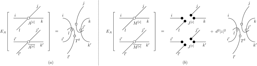
Figure 2: (a) The expectation of the product of $A^{[v]}$ and its conjugate is a product of delta tensors. (b) The expectation of the product $M^{[v]}\otimes\overline{M^{[v]}}$ decomposes into a linear combination of delta tensors and a product of rank-$1$ tensors.

Proof.

As in Figure 2 (a), we label the free edges of the first copy of $A^{[v]}$ by $i,j,k,l$, and the free edges of the second copy by $i^{\prime},j^{\prime},k^{\prime},l^{\prime}$. By definition, all entries of $A^{[v]}$ are sampled independently from $\mathcal{N}_{\mathbb{C}}(0,1)$. Thus, we have that

$$\left(E_{A}\left[A^{[v]}\otimes\overline{A^{[v]}}\right]\right)_{ijkl,i^{\prime}j^{\prime}k^{\prime}l^{\prime}}=\delta_{ii^{\prime}}\cdot\delta_{jj^{\prime}}\cdot\delta_{kk^{\prime}}\cdot\delta_{ll^{\prime}},$$ (58)

which proves Eq. (56). To prove Eq. (57), it suffices to notice that

$$M^{[v]}=J^{[v]}+zd\cdot A^{[v]}.$$ (59)

$$E_{A}\left[J^{[v]}\otimes\overline{A^{[v]}}\right]=E_{A}\left[A^{[v]}\otimes\overline{J^{[v]}}\right]=0.$$ (60)

∎

Proof of Lemma 19.

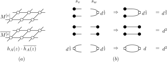
Figure 3: (a) Pair the tensors $M^{[v]}$ and its conjugate in $E_{A}|g_{A}(z)|^{2}.$ (b) The tensors with respect to edge $(v,w)$ in $T(s)$. From top to button, the value of $(s_{v},s_{w})$ are $(1,-1),(1,1),(-1,-1)$ respectively.

As in Figure 3 (a), $h_{A}(z)\cdot\overline{h_{A}(z)}$ is the product of two 2D tensor network, where for each vertex $v$, we can pair the tensors as $M^{[v]}\otimes\overline{M^{[v]}}$. By Lemma 20 we know that

$$N^{[v]}\coloneqq E_{A}\left[M^{[v]}\otimes\overline{M^{[v]}}\right]=J^{[v]}\otimes J^{[v]}+|z|^{2}(d^{1/2}\cdot T^{\delta})^{\otimes 4}.$$ (61)

Define a new 2D tensor network $T(N)$ where at each vertex $v$ the tensor is $N^{[v]}$. Notice that $E_{A}|h_{A}(z)|^{2}=\chi(T(N))$ since

$$E_{A}|h_{A}(z)|^{2} =E_{A}\left(\sum_{c\in[d]^{|E|}}\prod_{v\in V}M_{c}^{[v]}\right)\left(\sum_{c\in[d]^{|E|}}\prod_{v\in V}\overline{M_{c}^{[v]}}\right)$$ (62)

$$=\sum_{c,c^{\prime}\in[d]^{|E|}}\prod_{v\in V}E_{A}\left(M^{[v]}\otimes\overline{M^{[v]}}\right)_{c,c^{\prime}}$$ (63)

$$=\chi(T(N)).$$ (64)

We map $\chi(T(N))$ to the partition function of the 2D Ising model as follows. For any configuration $s\coloneqq\{s_{v}\}_{v\in V}$, $s_{v}\in\{\pm 1\}$, construct a new 2D tensor network $T(s)$ as follows:

• If $s_{v}=1$ we set the tensor on $v$ to be $J^{[v]}\otimes J^{[v]}$;

• If $s_{v}=-1$ we set the tensor on $v$ to be $(d^{1/2}\cdot T^{\delta})^{\otimes 4}$.

As in the top figure in Figure 3 (b), for an edge $(v,w)$, if $(s_{v},s_{w})=(1,-1)$, then the edge $(v,w)$ contributes a scalar factor as $d^{\frac{3}{2}}$ to $T(s)$, which is the contraction value of the tensor $J^{[v]}\otimes J^{[v]}$ and the tensor $(d^{1/2}\cdot T^{\delta})^{\otimes 4}$. Similarly, as in Figure 3 (b), if $(s_{v},s_{w})=(1,1)$ or $(-1,-1)$, the edge $(v,w)$ contributes a scalar factor as $d^{2}$. Thus

one can check that the contraction value of $T(s)$ is given by $R(s)$.

With an arbitrary ordering of the $n$ vertices, we write the configuration $s=\{s_{v}\}_{v\in V}$ as a vector $s\in\{\pm 1\}^{n}$. Based on Eq. (61), one can compute $\chi(T(N))$ by expanding $N^{[v]}$, that is for any configuration $s$,

• We use $s_{v}=1$ to represent choosing $J^{[v]}\otimes J^{[v]}$,

• We use $s_{v}=-1$ for $|z|^{2}\cdot(d^{1/2}\cdot T^{\delta})^{\otimes 4}$.

Then define $|s|$ to be the number of $-1$ in $s$, we have

$$\chi(T(N))=\sum_{s\in\{\pm 1\}^{n}}\chi(T(s))|z|^{2|s|}=\sum_{s\in\{\pm 1\}^{n}}R(s)|z|^{2|s|}$$ (65)

One can check that setting $\beta\mathcal{J}=\frac{\ln d}{4}$ and $\beta\varrho=\ln|z|$, for any $s\in\{\pm 1\}^{n}$, we have

$$d^{7n/2}|z|^{n}\exp(-\beta H(s,\mathcal{J},\varrho))=R(s)|z|^{2|s|}.$$ (66)

∎

5.4 Finding a root-free strip

In this section, we show that one can efficiently find a root-free strip with high probability. In particular, we will bound $E_{A}[|h_{A}(z)|^{2}]$ and use Lemma 11.

Recall that we consider a 2D lattice with periodic boundary conditions, where the 2D lattice has size $n=L_{1}\times L_{2}$ and $L_{2}$ is even. The 2D Ising model and $R(s)$ are defined in Section 5.2.

The exact formula for the partition function $\mathcal{Z}(\beta,\mathcal{J},0)$ in Lemma 18 is intimidating. We upper bound $\mathcal{Z}(\beta,\mathcal{J},0)$ by a simpler formula. Then we will use this formula to bound $E_{A}[|h_{A}(z)|^{2}]$.

Lemma 21 (Bound on the partition function with no magnetic field).

If $\beta\mathcal{J}=1/4\cdot\ln d$ and $d\geq 3$, we have that

$$2d^{\frac{n}{2}}\leq\mathcal{Z}(\beta,\mathcal{J},0)\leq 2d^{\frac{n}{2}}\left(1+\frac{3}{d}\right)^{n}$$ (67)

Proof.

Here we use the same notation as in Lemma 18. By the definition of the partition function, and the fact that there are $2n$ edges in the 2D square lattice with periodic boundary conditions, we have

$$\mathcal{Z}(\beta,\mathcal{J},0)\geq\sum_{s=00..0\text{ or }11\ldots 1}\prod_{(v,w)\in E}\exp(\beta\mathcal{J}s_{v}s_{w})=2d^{n/2}.$$ (68)

Now, note that we can rewrite the definitions in Lemma 18, for any $j$ as

$$2\cosh\gamma_{j}=\cosh 2H^{*}\cdot 2\cosh 2\beta\mathcal{J}\cdot\left(1-\alpha\cos(j\pi/L_{2})\right),,$$ (69)

where $\alpha\coloneqq\tanh 2H^{*}\cdot\tanh 2\beta\mathcal{J}\in(0,1)$. Since $L_{2}$ is even, we have

$$\prod_{r=1}^{L_{2}}(1-\alpha\cos(2r\pi/L_{2})) =\prod_{r=1}^{L_{2}/2}\left(1-\alpha\cos(2r\pi/L_{2})\right)\left(1-\alpha\cos(2(r+\frac{L_{2}}{2})\pi/L_{2})\right)$$ (70)

$$=\prod_{r=1}^{L_{2}/2}\left(1-\alpha\cos(2r\pi/L_{2})\right)\left(1+\alpha\cos(2r\pi/L_{2})\right)$$ (71)

$$=\prod_{r=1}^{L_{2}/2}\left(1-\alpha^{2}\cos^{2}(2r\pi/L_{2})\right)$$ (72)

$$\leq 1.$$ (73)

By the definition of $\cosh$, $2\cosh kx\leq(2\cosh x)^{k}$ for any $x$ and any integer $k\geq 0$, we have that

$$\prod_{r=1}^{L_{2}}\left(2\cosh\frac{L_{1}}{2}\gamma_{2r}\right) \leq\left(\prod_{r=1}^{L_{2}}2\cosh\gamma_{2r}\right)^{L_{1}/2}$$ (74)

$$=\left(\cosh 2H^{*}\cdot 2\cosh 2\beta\mathcal{J}\right)^{L_{1}L_{2}/2}\left(\prod_{r=1}^{L_{2}}(1-\alpha\cos(2r\pi/L_{2}))\right)^{L_{1}/2}$$ (75)

$$\leq\left(\cosh 2H^{*}\cdot 2\cosh 2\beta\mathcal{J}\right)^{L_{1}L_{2}/2}.$$ (76)

where the second equality comes from Eq. (69) and the last inequality comes from Eq. (73). Similarly we can get the same upper bound for

$$\prod_{r=1}^{L_{2}}\left(2\cosh\frac{L_{1}}{2}\gamma_{2r-1}\right),\text{ and }\prod_{r=1}^{L_{2}}\left(2\sinh\frac{L_{1}}{2}\gamma_{2r}\right),\prod_{r=1}^{L_{2}}\left(2\sinh\frac{L_{1}}{2}\gamma_{2r-1}\right).$$

where we get the bound for the last two terms by $|\sinh x|\leq\cosh x$. Besides, from $\tanh H^{*}=\exp(-2\beta\mathcal{J})$ we have

$$\exp(2H^{*})=\frac{\exp(2\beta\mathcal{J})+1}{\exp(2\beta\mathcal{J})-1}=\frac{\sqrt{d}+1}{\sqrt{d}-1}$$ (77)

$$\cosh 2H^{*}=\frac{1}{2}\left(\frac{\sqrt{d}+1}{\sqrt{d}-1}+\frac{\sqrt{d}-1}{\sqrt{d}+1}\right)\leq 1+\frac{3}{d},\text{ for }d\geq 3.$$ (78)

We estimate

$$2\sinh 2\beta\mathcal{J}=\sqrt{d}-\frac{1}{\sqrt{d}}\leq\sqrt{d}.$$ (79)

$$2\cosh 2\beta\mathcal{J}=\sqrt{d}+\frac{1}{\sqrt{d}}$$ (80)

Thus by Lemma 18, we finally conclude that

$$\mathcal{Z}(\beta,\mathcal{J},0) \leq\frac{1}{2}\cdot d^{\frac{n}{4}}\cdot 4\cdot\left(1+\frac{3}{d}\right)^{\frac{n}{2}}d^{\frac{n}{4}}\left(1+\frac{1}{d}\right)^{\frac{n}{2}}$$ (81)

$$\leq 2d^{\frac{n}{2}}\left(1+\frac{3}{d}\right)^{n}.$$ (82)

∎

Using Lemma 21 we can now estimate $\sum_{s}R(s)$.

Lemma 22.

$$\sum_{s\in\{\pm 1\}^{n}}R(s)\leq 2d^{4n}(1+\frac{3}{d})^{n}$$ (83)

Proof.

Since the 2D lattice we consider has $n$ vertices and satisfies the periodic boundary condition, there are in total $2n$ edges. Set $z=1,\beta\mathcal{J}=1/4\cdot\ln d$, $\beta\varrho=\ln|z|=0$, (that is $\varrho=0$). By Lemma 19 and Lemma 21 we have that

$$\sum_{s\in\{\pm 1\}}R(s) =d^{7n/2}\mathcal{Z}(\beta,\mathcal{J},0)\leq 2d^{4n}\left(1+\frac{3}{d}\right)^{n}.$$ (84)

∎

Then we estimate $E_{A}|h_{A}(z)|^{2}$ for small $z$ and for $z\leq 1$. For completeness we also give a lower bound on $E_{A}|h_{A}(z)|^{2}$ in Lemma 23 (c). (c) will not be used in other proofs.

Lemma 23.

Let $c$ and $\rho$ be two constants where $0<\rho<1$. Assume $d\geq nc^{-1}$.We have

• For $|z|\leq\rho$, $E_{A}|h_{A}(z)|^{2}\leq d^{4n}(1+2\rho^{2}e^{3c}).$

• For $|z|\leq 1,$ $E_{A}|h_{A}(z)|^{2}\leq d^{4n}\cdot 2e^{3c}.$

• For any $z$, $E_{A}|h_{A}(z)|^{2}\geq d^{4n}(1+\frac{|z|^{2}}{d^{4}})^{n}$.

Proof.

Note that when $s=0\ldots 0$, $R(s)=d^{4n}$. For (a), since $|z|\leq\rho$, by Lemma 19 we have

$$E_{A}|h_{A}(z)|^{2} =d^{4n}\cdot|z|^{0}+\sum_{s\in\{\pm 1\}^{n}:|s|\geq 1}R(s)|z|^{2s}$$ (85)

$$\leq d^{4n}+\rho^{2}\sum_{s\in\{\pm 1\}^{n}}R(s)$$ (86)

$$\leq d^{4n}+\rho^{2}\cdot 2d^{4n}\left(1+\frac{3}{d}\right)^{n}$$ (87)

$$\leq d^{4n}(1+2\rho^{2}e^{3c}).$$ (88)

where the second inequality comes from $|z|\leq\rho<1$ and $R(s)\geq 0,\forall s$; the third inequality comes from Lemma 22; and the last inequality comes from $d\geq n\cdot c^{-1}$.

For (b), by Lemma 19 and Lemma 22 we have for $|z|\leq 1$,

$$E_{A}|h_{A}(z)|^{2} \leq\sum_{s\in\{\pm 1\}^{n}}R(s)\cdot 1$$ (89)

$$\leq d^{4n}2\left(1+\frac{3}{d}\right)^{n}$$ (90)

$$\leq d^{4n}\cdot 2e^{3c}.$$ (91)

For (c), note that for $|s|=k$, since there are at most $4k$ edges $(v,w)$ in $R(s)$ which take values $r_{vw}(s)=d\sqrt{d}$, we must have $R(s)\geq d^{4n}/\sqrt{d}^{4k}$. Thus

$$E_{A}|h_{A}(z)|^{2} =\sum_{k=0}^{n}\sum_{s\in\{\pm 1\}^{n}:|s|=k}R(s)|z|^{2k}.$$ (92)

$$\geq\sum_{k=0}^{n}\binom{n}{k}d^{4n}\left(\frac{|z|^{2}}{d^{2}}\right)^{k}$$ (93)

$$=d^{4n}\left(1+\frac{|z|^{2}}{d^{2}}\right)^{n}.$$ (94)

∎

Recall that $N_{A}(r)$ is the number of roots of $h_{A}(z)$ inside the disk $\mathcal{B}(r)$. With Lemma 23, we can estimate $N_{A}(r)$ by using Lemma 11.

Corollary 24.

Suppose $d\geq nc^{-1}$ for some constant $c$. Let $\lambda$ be an arbitrary small constant satisfying $0\leq\lambda\leq\min\{1/80,e^{-3c}/80\}$. We have

$$Pr_{A}\left[N_{A}(\lambda)=0\quad\&\quad N_{A}(1-\lambda)\leq\frac{1}{\lambda^{2}}\right]\geq 4/5.$$ (95)

Proof.

Note that

$$h_{A}(0)=d^{2n}.$$

We have

$$E_{A}[N_{A}(\lambda)] \leq E_{A}\left[N_{A}\left(2\lambda-2\lambda\cdot\lambda/2\right)\right]$$ (96)

$$\leq\frac{1}{\lambda}\ln E_{\theta}E_{A}\frac{|h_{A}(2\lambda\cdot e^{i\theta})|^{2}}{|h_{A}(0)|^{2}}$$ (97)

$$\leq\frac{1}{\lambda}\cdot\ln(1+8\lambda^{2}e^{3c})$$ (98)

$$\leq 8\lambda\cdot e^{3c};$$ (99)

where the first inequality comes from the fact that the disk of radius $2\lambda-2\lambda\cdot\lambda/2$ contains the disk of radius $\lambda$; the second inequality comes from Lemma 11; and the third inequality comes from Lemma 23 (a) by setting $\rho=2\lambda$.

Similarly from Lemma 11 and Lemma 23 (b) we get

$$E_{A}\left[N_{A}\left(1-\lambda\right)\right] \leq\frac{1}{2\lambda}\ln E_{\theta}E_{A}\frac{|h_{A}(e^{i\theta})|^{2}}{|h_{A}(0)|^{2}}$$ (100)

$$\leq\frac{1}{2\lambda}\cdot\ln(2e^{3c}).$$ (101)

Then by Markov inequality, we have

$$Pr_{A}\left[N_{A}(\lambda)\geq 1\right] \leq E_{A}\left[N_{A}(\lambda)\right]$$ (102)

$$\leq 8\lambda\cdot e^{3c}$$ (103)

$$\leq\frac{1}{10}.$$ (104)

$$Pr_{A}\left[N_{A}\left(1-\lambda\right)\geq\frac{1}{\lambda^{2}}\right] \leq\lambda^{2}\cdot E_{A}\left[N_{A}(1-\lambda)\right]$$ (105)

$$\leq\lambda/2\cdot\ln(2e^{3c})$$ (106)

$$\leq\frac{1}{10}.$$ (107)

Then we get the desired result by a union bound. ∎

Finally we prove Lemma 17.

Proof of Lemma 17.

Let

$$M\coloneqq 1/\lambda^{3},\quad\theta\coloneqq 2\pi/M,\quad w\coloneqq\pi\lambda^{4}/2.$$ (108)

For simplicity we assume that $1/\lambda$ is an integer. Consider the disk $\mathcal{B}(1-\lambda)$, that is the disk centered at $0$ and of radius $1-\lambda$. As in Figure 4, we divide $\mathcal{B}(1-\lambda)$ into $M$ disjoint circular sectors, where for each sector the central angle is $\theta$. Insider each sector which is indexed by $k\in[M]$, we consider a strip of width $w$, that is

$$\mathcal{T}_{k}\coloneqq\mathcal{T}((1-2\lambda)e^{ik\theta},w).$$

Note that since $\sin x\geq x/2$ for $0\leq x\leq\pi/3$, we have

$$\lambda\sin\left(\theta/2\right)\geq\lambda\theta/4=\pi\lambda^{4}/2=w.$$ (109)

Thus all the $M$ strips $\{\mathcal{T}_{k}\}_{k=1}^{M}$ are disjoint outside $\mathcal{B}(\lambda)$. Besides, one can check that the end part of the strip $\mathcal{T}_{k}$ is inside the $k$-th sector by noticing

$$0\leq\lambda\leq 1/80\Rightarrow(1-2\lambda)\tan\frac{\theta}{2}\geq w.$$

Denote $S_{good}$ as the set of tensors $A$ which have no roots in the disk of radius $\lambda$ and few roots in the disk of radius $1-\lambda$:

$$S_{good}\coloneqq\{A:\quad N_{A}(\lambda)=0\,\,\&\,\,N_{A}(1-\lambda)\leq\frac{1}{\lambda^{2}}\}.$$

By Corollary 24, we know that

$$Pr_{A}\left[A\in S_{good}\right]\geq 4/5.$$ (110)

In the following we argue that $S_{good}$ can be further partitioned into disjoint subsets, where in each subset, with probability at least $(1-\lambda)$ over the randomness of $A$ there are no roots in $\mathcal{T}(1-2\lambda,w)$.

To this end, first we observe that for any $k\in[M]$, by the definition of $h_{A}(\cdot)$, we have

$$h_{e^{ik\theta}A}(z)=h_{A}(e^{ik\theta}z).$$ (111)

Note that $e^{ik\theta}z$ is just a rotation of $z$ in the complex plane. By the rotational symmetry of disks, the roots of $h_{e^{ik\theta}A}(z)=h_{A}(e^{ik\theta}z)$ are simply rotated compared to the roots of $h_{A}(z)$. Thus if $A\in S_{good}$, then so is $e^{ik\theta}A$.

Next, we partition $S_{good}$ into disjoint subsets in the way that $A,A^{\prime}$ are in the same subset iff there exists $k\in[M]$ such that $A^{\prime}=e^{ik\theta}A$. For convenience, for each subset we fix an arbitrary $A$ as the representative and write the subset as

$$S_{good}(A)=\{e^{ik\theta}A|\,k\in[M]\}.$$

By the definition of $S_{good}$, for any $A\in S_{good}$, there are no roots in $\mathcal{B}(\lambda)$ and there are at most $1/\lambda^{2}$ roots in $\mathcal{B}(1-\lambda)$. Since the $M$ tubes $\{\mathcal{T}_{k}\}_{k=1}^{M}$ are disjoint outside $\mathcal{B}(\lambda)$, there is at most a $\frac{1/\lambda^{2}}{M}=\lambda$ fraction of the $M$ tubes which contains roots of $h_{A}(z)$. Further, recall that

$$h_{e^{ik\theta}A}(z)=h_{A}(e^{ik\theta}z),$$

and thus the tube $\mathcal{T}_{0}$ with respect to to $e^{ik\theta}A$ corresponds to the tube $\mathcal{T}_{k}$ with respect to $A$. Hence, there is at most a $\lambda$ fraction of $A^{\prime}\in S_{good}(A)$ such that the corresponding strip $\mathcal{T}_{0}$ contains roots of $h_{A}(z)$.

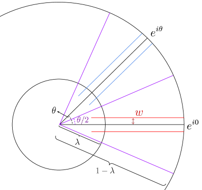
Figure 4: The radius of the small disk and the big disk is $\lambda$ and $1-\lambda$ respectively. We divide the big disk $\mathcal{B}(1-\lambda)$ into $M$ circular sectors. In each sector we choose a strip of width $w$. The first strip $\mathcal{T}_{0}$ starts from $-w$ and ends at $1-2\lambda+w$. Other strips are rotations of $\mathcal{T}_{0}$. All the strips are disjoint outside the small disk $\mathcal{B}(\lambda)$.

In summary, we conclude that the fraction of $A$ such that there are no roots in $\mathcal{T}(1-2\lambda,w)$ is greater than

$$\frac{4}{5}\cdot(1-\lambda)\geq\frac{3}{4}+\frac{1}{25}.$$

∎

5.5 $\#\mbox{\bf P}$-hardness of exact contraction

Finally we prove that the exact contraction of the random 2D tensor network with a positive mean remains $\#\mbox{\bf P}$-hard. The proof is a simple adaption of Theorem 1 and Theorem 3 in [HHEG20]. For completeness, we put a proof in Appendix A.

To make the statement rigorous, here we consider the finite precision approximation of the Gaussian distribution, denoted as $\overline{\mathcal{N}}_{\mathbb{C}}(\mu,\sigma^{2})$, where each sample can be represented by finite bits instead of being an arbitrary real or complex number. For example here we set the $\overline{\mathcal{N}}_{\mathbb{C}}(\mu,\sigma^{2})$ to be the distribution where each sample $z\sim\overline{\mathcal{N}}_{\mathbb{C}}(\mu,\sigma^{2})$ is obtained by: firstly sample $y$ according to Gaussian distribution $\mathcal{N}_{\mathbb{C}}(\mu,\sigma^{2})$, then set $z$ to be the value by rounding $y$ to $n^{2}$ bits. $\overline{\mathcal{N}}_{\mathbb{C}}(\mu,\sigma^{2})$ behaves similarly as $\mathcal{N}_{\mathbb{C}}(\mu,\sigma^{2})$ but makes the statements of exact contraction and proofs more rigorous.

Accordingly, we consider finite precision 2D $(\mu,n,d)$-Gaussian tensor network instead of 2D $(\mu,n,d)$-Gaussian tensor network, where we substitute $\mathcal{N}_{\mathbb{C}}(\mu,\sigma^{2})$ by $\overline{\mathcal{N}}_{\mathbb{C}}(\mu,\sigma^{2})$.

Theorem 25 ($\#\mbox{\bf P}$-hard).

For any $\mu\in[0,poly(n)]$, $n\geq 25$ and $d=O(poly(n))$, if there exists an algorithm $\mathcal{A}$ which runs in $poly(n)$ time and with probability at least $\frac{3}{4}+\frac{1}{n}$ over the randomness of the finite precision 2D $(\mu,n,d)$-Gaussian tensor network $T$, it outputs the exact value of $\chi(T)$, then there exists an algorithm which runs in randomized $poly(n)$ time and solves $\#\mbox{\bf P}$-complete problems.

6 Approximating arbitrary positive tensor networks

In previous sections we have considered approximating random tensor networks. In this section we move to the task of contracting a fixed tensor network.

For a general tensor network $T=T(G,M)$, computing the contraction value $\chi(T)$ exactly is known to be $\#\mbox{\bf P}$-hard [SWVC07]. On the other hand, Arad and Landau [AL10] proved that approximating $\chi(T)$ up to an inverse polynomial additive error in the matrix $2$-norm is BQP-complete.

In this section, we focus on positive tensor network $T=T(G,M)$. These are defined by tensors $\{M^{[v]}\}_{v}$ the entries of which are all non-negative. The main part of this section will establish that when $T$ is a positive tensor network, approximating $\chi(T)$ up to an inverse polynomial additive error in the matrix $1$-norm is BPP-complete. Then, in Section 6.4 we give a short proof showing that approximating positive tensor network with inverse-poly multiplicative error is at least StoqMA-hard. Section 6.4 is self-contained and can be read independently. We first review the swallowing algorithm for tensor network contraction. Then we explain Arad and Landau’s BQP-completeness result and our BPP-completeness result, which are both based on the swallowing algorithm.

6.1 A swallowing algorithm and notations

Recall that in Section 2 we have introduced two operations on tensor networks, taking their product and contraction. Given a tensor network $T=T(G,M)$, the swallowing algorithm (Algorithm 2) is a standard method to exactly compute the contraction value $\chi(T)$, by contracting edges of tensors $\{M^{[v]}\}_{v}$ according to the graph $G=(V,E)$.

Algorithm 2 The swallowing algorithm

1:Given an ordering of vertex $v_{1},\ldots,v_{n}$ of $G$.

2:Set $i\leftarrow 1$. Set the current tensor $A[i]$ to be the tensor $M^{[v_{1}]}$, which can be pictured as one vertex and some free edges as in Figure 1 (a).

3:while $i\leq n$ do $\triangleright$ Adding tensor $M^{[v_{i+1}]}$ to $A[i]$

4:     if $M^{[v_{i+1}]}$ and $A[i]$ share edges in $G$ then

5:         Construct a new tensor $A[i+1]$ by contraction, i.e. identifying the shared edges and summing over the corresponding indices.

6:     else

7:         $M^{[v_{i+1}]}$ and $A[i]$ has no common edge.

8:         Then $A[i+1]$ is defined as the product $M^{[v_{i+1}]}\otimes A[i]$.

9:     end if

10:     $i\leftarrow i+1$

11:end while

12:return $\chi(T)\leftarrow A[n]$

High level ideas for Arad and Landau’s result and our result. Let us first describe Arad and Landau’s result at a high level before writing down formal statements with heavy notations. As in Figure 5, given an arbitrary ordering to the vertices, for every vertex $v_{i}$, we implicitly partition the free edges of $M^{[v_{i}]}$ into input and output edges. With respect to this partition of in-edges and out-edges, one can write $M^{[v_{i}]}$ as a matrix denoted as $M^{[v_{i}]in,out}$. As in Algorithm 2, the contraction value of the tensor network is then given by sequentially mapping the in-edges to out-edges, which can be represented by the matrix multiplication $\prod_{i}M^{[v_{i}]in,out}\otimes I_{else}$, where $I_{else}$ denotes the free edges other than the input edges in $A[i-1]$. Arad and Landau’s result shows that this matrix multiplication can be simulated by a quantum circuit through embedding each matrix $M^{[v_{i}]in,out}$ into a unitary, where the embedding is done by adding an ancillary qubit. Our result is, when every $M^{[v_{i}]in,out}$ is a positive matrix, instead of embedding it into a unitary, we embed the positive matrix into a stochastic matrix and simulate positive matrix multiplication with a random walk.

To explain Arad and Landau’s result formally, we define more notation which is used in the swallowing algorithm. This notation is adapted from [AL10].

Figure 5: $F_{i}$ is the edges connecting $\{v_{1},...,v_{i-1}\}$ and $\{v_{i},...,v_{n}\}$. The edges attached to $v_{i}$ are partitioned into the in-edges $K_{i}$ and out-edges $L_{i}$. When contracting the tensor $M^{[v_{i}]}$ we map the in-edges to out-edges. The edges in $F_{i}$ but not in $K_{i}$ are called $J_{i}$.

As in Figure 5, define

• $S_{i}=\{v_{1},\ldots,v_{i}\}$.

• $F_{i}$ is the set of edges which connect $S_{i-1}$ and $V/S_{i-1}$. $F_{i}$ are the free edges in tensor $A[i-1]$.

• $K_{i}$ is the set of edges which connects $S_{i-1}$ and $v_{i}$. $K_{i}$ are the edges being contracted when contracting $A[i-1]$ and $M^{[v_{i}]}$. Note that $K_{1}=\emptyset$.

• $J_{i}\coloneqq F_{i}/K_{i}$, which are the free edges in both $A[i-1]$ and $A[i]$. $J_{1}=\emptyset$.

• $L_{i}$ is the set of edges of $v_{i}$ which are not in $K_{i}$. In other words, $L_{i}$ are the new free edges introduced by adding tensor $M^{[v_{i}]}$ to $A[i-1]$.

Denote edges in $K_{i}$ as $\{e^{K_{i}}_{1},\ldots,e^{K_{i}}_{|K_{i}|}\}$. Denote edges in $J_{i}$ and $L_{i}$ similarly. With some abuse of notations, we use $e^{K_{i}}_{s}$ to denote both the name of the edge and the colors in $[d]$ that the edge $e^{K_{i}}_{s}$ takes.

In the following, we explain that the update from tensors $A[i-1]$ to $A[i]$ can be written as matrix multiplication. More specifically:

• First note that $A[i]$ can be viewed as a column vector consisting of $d^{|F_{i+1}|}$ entries, where the entries are indexed by the free edges of $A[i]$, that is

  $$F_{i+1}=K_{i+1}\cup J_{i+1}=L_{i}\cup J_{i}.$$

  More specifically, write this vector as $\left|A[i]\right\rangle\in\mathbb{C}^{d^{|F_{i+1}|}}$, then for edges in $J_{i},L_{i}$ taking colors as $e^{J_{i}}_{1},\ldots,e^{J_{i}}_{|J_{i}|},e^{L_{i}}_{1},\ldots,e^{L_{i}}_{|L_{i}|}$ where $e^{J_{i}}_{s},e^{L_{i}}_{t}\in[d]$, we define

  $$\left\langle e^{J_{i}}_{1},\ldots,e^{J_{i}}_{|J_{i}|},e^{L_{i}}_{1},\ldots,e^{L_{i}}_{|L_{i}|}\bigg{|}A[i]\right\rangle\coloneqq A[i]_{e^{J_{i}}_{1},\ldots,e^{J_{i}}_{|J_{i}|},e^{L_{i}}_{1},\ldots,e^{L_{i}}_{|L_{i}|}}.$$ (112)

• Note that $M^{[v_{i}]}$ can be viewed as a matrix: When adding $M^{[v_{i}]}$ to $A[i-1]$ in Line 5 of Algorithm 2, we contract the free edges in $K_{i}$ and introducing new free edges $L_{i}$. One can view $M^{[v_{i}]}$ as a mapping from $\mathbb{C}^{d^{|K_{i}|}}$ to $\mathbb{C}^{d^{|L_{i}|}}$, denoted as $M^{[v_{i}]K_{i}L_{i}}$, which can be written as a matrix of size $d^{|L_{i}|}\times d^{|K_{i}|}$ where

  $$\left\langle e^{L_{i}}_{1},\ldots,e^{L_{i}}_{|L_{i}|}\bigg{|}M^{[v_{i}]}\bigg{|}e^{K_{i}}_{1},\ldots,e^{K_{i}}_{|K_{i}|}\right\rangle=M^{[v_{i}]}_{e^{L_{i}}_{1},\ldots,e^{L_{i}}_{|L_{i}|},e^{K_{i}}_{1},\ldots,e^{K_{i}}_{|K_{i}|}}$$ (113)

  In particular, since $K_{1}=\emptyset$, $M^{[v_{i}]K_{i}L_{i}}$ is a column vector in $\mathbb{C}^{d^{|L_{1}|}}$. For convenience, define $\left|A[0]\right\rangle$ to be a scalar,

  $$\left|A[0]\right\rangle\coloneqq 1.$$

  Denote $I_{J_{i}}$ as the identity operator on the indices with respect to edges in $J_{i}$.

• One can check that the updates from $A[i-1]$ to $A[i]$ can be written as matrix multiplication, that is for $i=1,\ldots,n,$

  $$\left|A[i]\right\rangle=I_{J_{i}}\otimes M^{[v_{i}]K_{i}L_{i}}\left|A[i-1]\right\rangle,$$ (114)

  in the sense that

  $$\left\langle e^{J_{i}}_{1},\ldots,e^{J_{i}}_{|J_{i}|},e^{L_{i}}_{1},\ldots,e^{L_{i}}_{|L_{i}|}\bigg{|}A[i]\right\rangle$$

  $$=\sum_{e^{K_{i}}_{1},\ldots,e^{K_{i}}_{|K_{i}|}}\left\langle e^{L_{i}}_{1},\ldots,e^{L_{i}}_{|L_{i}|}\bigg{|}M^{[v_{i}]}\bigg{|}e^{K_{i}}_{1},\ldots,e^{K_{i}}_{|K_{i}|}\right\rangle\left\langle e^{K_{i}}_{1},\ldots,e^{K_{i}}_{|K_{i}|},e^{J_{i}}_{1},\ldots,e^{J_{i}}_{|J_{i}|}\bigg{|}A[i-1]\right\rangle.$$ (115)

  In particular, $\left|A[n]\right\rangle$ is a scalar which equals to the contraction value. Thus we have

  $$\left|A[n]\right\rangle=\prod_{i=1}^{n}I_{J_{i}}\otimes M^{[v_{i}]K_{i}L_{i}}=\chi(T).$$ (116)

To ease notations we define the swallowing operator as

$$O^{[v_{i}]}\coloneqq I_{J_{i}}\otimes M^{[v_{i}]K_{i}L_{i}}.$$ (117)

6.2 BPP-completeness of additive-error approximation

According to the discussion in the previous section, one can compute $\chi(T)$ exactly by updating $\left|A[i]\right\rangle$ according to Eq. (114). It is well known that computing $\chi(T)$ exactly is $\#\mbox{\bf P}$-hard even for a constant degree graph $G$, thus one cannot efficiently perform the exact version of the update Eq. (114). However, interestingly [AL10] showed that one can approximately perform the update efficiently using a quantum computer, where the approximation refers to an inverse polynomial additive error in the 2-norm of the tensors.

Theorem 26 (Additive $2$-norm approximation of tensor networks [AL10]).

Let $G=(V,E)$ be an $n$-vertex graph of constant degree. Let $T(G,M)$ be a tensor network on $G$ with bond dimension $d=O(poly(n))$. The following approximation problem is BQP-complete: Given as input

• a tensor network $T(G,M)$, and a precision parameter $\epsilon=1/poly(n)$, and

• an ordering of the vertices $v_{1},\ldots,v_{n}$, and the corresponding swallowing operators $O^{[v_{i}]}$ defined in Eq. (117),

output a complex number $\hat{\chi}(T)$ such that

$$Pr\left(|\chi(T)-\hat{\chi}(T)|\leq\epsilon\Delta_{2}\right)\geq 3/4,$$ (118)

where

$$\Delta_{2}\coloneqq\prod_{i=1}^{n}\|O^{[v_{i}]}\|_{2}.$$ (119)

Note that by Eq. (117), both the 2-norm $\|\cdot\|_{2}$ and 1-norm of $\|\cdot\|_{1}$ of $O^{[v_{i}]}$ equal to the corresponding norm of $M^{[v_{i}]K_{i}L_{i}}$.

We prove that if the tensor network $T$ is a positive tensor network, then instead of using a quantum computer, we can approximate the update Eq. (114) efficiently using a classical computer, where the approximation refers to an inverse polynomial additive error in the matrix $1$-norm of the matrices $O^{[v_{i}]}$.

Theorem 27 (Additive $1$-norm approximation of positive tensor networks).

Let $G=(V,E)$ be an $n$-vertex graph of constant degree. Let $T(G,M)$ be a positive tensor network on $G$ with bond dimension $d=O(poly(n))$. The following approximation problem is BPP-complete: Given as input

• a positive tensor network $T(G,M)$, and a precision parameter $\epsilon=1/poly(n)$, and

• an ordering of vertices $v_{1},\ldots,v_{n}$, and the corresponding swallowing operators $O^{[v_{i}]}$ defined in Eq. (117),

output a complex number $\hat{\chi}(T)$ such that

$$Pr\left(|\chi(T)-\hat{\chi}(T)|\leq\epsilon\Delta_{1}\right)\geq 3/4,$$ (120)

where

$$\Delta_{1}\coloneqq\prod_{i=1}^{n}\|O^{[v_{i}]}\|_{1}.$$ (121)

6.3 Proof of Theorem 27

The proof of the BPP-hardness part for Theorem 27 is similar to Section 4.2 in [AL10]. For completeness we give a proof sketch in Appendix C. In the following we prove the “inside BPP” part of Theorem 27, that is, we provide an efficient classical algorithm that achieves Eq. (120). The main idea of the algorithm is to simulate non-negative matrix multiplication via a stochastic process.

We say that a matrix is non-negative if all of its entries are non-negative. We first give a lemma which extends a non-negative matrix to a stochastic matrix.

Lemma 28.

Let $M\neq 0$ be a non-negative matrix, that is $M\in\mathbb{R}_{\geq 0}^{m\times n}$. Then there exists $N\in\mathbb{R}_{\geq 0}^{2m\times n}$ such that $N$ is a stochastic matrix, and $\frac{M}{\|M\|_{1}}$ is the first $m$ rows of $N$.

Proof.

Since $\|M\|_{1}=\max_{1\leq j\leq n}\sum_{i=1}^{m}|M_{ij}|,$ thus for each column, the column sum of $\frac{M}{\|M\|_{1}}$ lies in $[0,1]$, thus one can embed $\frac{M}{\|M\|_{1}}$ as the first $m$ rows in a stochastic matrix $N$. ∎

Before we state the BPP algorithm, we recall some notations. Recall that we have defined $F_{i},J_{i},K_{i},L_{i},A[i],M^{[v_{i}]K_{i}L_{i}}$ in Section 6.1 and Figure 5. To ease notation, we abbreviate $M^{[v_{i}]K_{i}L_{i}}$ as $M^{[v_{i}]}$. Since we are working with positive tensor network, $M^{[v_{i}]}$ is a non-negative matrix and the entries are indexed by $K_{i},L_{i}$.

Lemma 28 says that we can embed $M^{[v_{i}]}/\|M^{[v_{i}]}\|_{1}$ in a stochastic matrix $N^{[v_{i}]}$ by adding one ancillary bit, that is $N^{[v_{i}]}$ is indexed by $L_{i}\cup\{w_{i}\}$ and $K_{i}$, where $w_{i}\in\{0,1\}$ is an index such that $w_{i}=0$ (or 1) refers to the first (or second) $d^{|L_{i}|}$ rows of $N^{[v_{i}]}$. Define

$$W_{i}\coloneqq\{w_{1},\ldots,w_{i-1}\}.$$ (122)

We first explain the high level idea of the BPP algorithm, and then give the pseudo code. The idea of the BPP algorithm in Theorem 27 is to mimic non-negative matrix multiplication by stochastic methods. From a high level idea, we will embed the vector $|A[i]\rangle$ in a probability distribution, and embed the matrix $M^{[v_{i}]}$ in a stochastic matrix $N^{[v_{i}]}$ by adding an ancillary bit. Then the update rule

$$\left|A[i+1]\right\rangle=I_{J_{i}}\otimes M^{[v_{i}]K_{i}L_{i}}\left|A[i]\right\rangle,$$ (123)

is embedded in applying the stochastic matrix $N^{[v_{i}]}$ to the distribution $A[i]$, which can be simulated by a random walk.

Before writing down the pseudo codes we explain some notations.

• We use $\left|k\right\rangle_{K}$ to represent the (ordered) coloring $k\in[d]^{|K|}$ of the edges in $K$. When $K=\emptyset$ we view $\left|k\right\rangle_{K}$ as empty, that is writing down nothing. Similarly for $\left|j\right\rangle_{J},\left|w\right\rangle_{W}$.

• We will use $s_{i}$ to denote a computational basis whose distribution embed the vector $A[i-1]$.

• Recall that the free edges of $A[i-1]$ are $F_{i}=K_{i}\cup J_{i}$. Also recall that $F_{i+1}=J_{i}\cup L_{i}$.

The pseudo codes are stated as Algorithm 3 and Algorithm 4. Their performance is given in Corollary 30.

Algorithm 3 Trial(T=T(G,M))

1:$i=1$, $s_{1}=\emptyset$.

2:while $i\leq n$ do

3:     Interpret $s_{i}=\left|k\right\rangle_{K_{i}}\left|j\right\rangle_{J_{i}}\left|w\right\rangle_{W_{i}}$. $\triangleright$ $K_{1}=J_{1}=W_{1}=\emptyset.$

4:     Recall that $N^{[v_{i}]}$ has rows indexed by $L_{i}\cup\{w_{i}\}$, column indexed by $K_{i}$.

5:     Since $N^{[v_{i}]}$ is a stochastic matrix, each column of $N^{[v_{i}]}$ corresponds to a distribution over the row index.

6:     if i=1 then

7:         $N^{[v_{1}]}$ is a column vector. Denote the distribution according to this column as $\mathcal{D}$.

8:     else

9:         Denote the distribution according to the $k$-th column of $N^{[v_{i}]}$ as $\mathcal{D}$.

10:     end if

11:     Sample a row index according to $\mathcal{D}$.

12:     Denote this row index as $\left|lw^{\prime}\right\rangle_{L_{i}\cup\{w_{i}\}}$, where $l\in[d]^{|L_{i}|},w^{\prime}\in\{0,1\}.$

13:     Set $s_{i+1}\leftarrow\left|l\right\rangle_{L_{i}}\left|j\right\rangle_{J_{i}}\left|ww^{\prime}\right\rangle_{W_{i+1}}$. $\triangleright$ $N^{[v_{i}]}$ maps register $K_{i}$ to $L_{i}\cup\{w_{i}\}$.

14:     $i\leftarrow i+1$.

15:end while

16:Interpret $s_{n+1}=\left|w\right\rangle_{W_{n+1}}$ $\triangleright$ We know $L_{n}=J_{n}=\emptyset$

17:Return Success if $w=00\ldots 00$, that is the all zero state; otherwise return Fail.

Algorithm 4 Approximating positive tensor network

1:Set $K=10\epsilon^{-2}$

2:Run the $Trial(T)$, that is Algorithm 3, for $K$ times.

3:Count the number of Success as $\#Success$.

4:Return $\hat{\chi}(T)\leftarrow\frac{\#Success}{K}\cdot\Delta_{1}$ as the approximation of $\chi(T)$.

Lemma 29.

The probability of the Trial algorithm (Algorithm 3) to return “Success” is $\chi(T)/\Delta_{1}$ where $\Delta_{1}\coloneqq\prod_{i=1}^{n}\|O^{[v_{i}]}\|_{1}$. Its runtime is $poly(n)$.

Proof.

To ease notation, for a set $Q\cup W$ where $Q$ is a set of edges of $G$, and $W$ is a set of ancillary indices $\{\ldots,w_{i},\ldots\}$, we use

$$String(Q\cup W)\coloneqq[d]^{|Q|}\times\{0,1\}^{|W|}$$

where edges/indices in $Q$ take values in $[d]$, and ancillary indices in $W$ takes values in $\{0,1\}$.

Define

$$S_{i}\coloneqq String(L_{i}\cup J_{i}\cup W_{i+1}),$$

define $\left|\pi_{i+1}\right\rangle$ as the probability distribution of $s_{i+1}$, which is a probability distribution over $S_{i}$. Note that

$$\left|\pi_{2}\right\rangle =I_{J_{1}}\otimes N^{[v_{1}]},\text{ where }I_{J_{1}}=I_{\emptyset}=1$$ (124)

$$\left|\pi_{i+1}\right\rangle =I_{J_{i}}\otimes N^{[v_{i}]}\left|\pi_{i}\right\rangle$$

$$=\prod_{h=1}^{i}I_{J_{h}}\otimes N^{[v_{h}]}$$ (125)

$$=\prod_{h=1}^{i}\frac{I_{J_{h}}\otimes M^{[v_{h}]}}{\|M^{[v_{h}]}\|_{1}}\left|0\ldots 0\right\rangle_{W_{i+1}}+\text{additional terms}$$ (126)

$$=\prod_{h=1}^{i}\frac{O^{[v_{h}]}}{\|O^{[v_{h}]}\|_{1}}\left|0\ldots 0\right\rangle_{W_{i+1}}+\text{additional terms}$$ (127)

where Eq. (125) is from Algorithm 3; Eq. (126) is from the definition of $N^{[v_{h}]}$ that $N^{[v_{h}]}$ embeds $M^{[v_{h}]}$; and the last equality comes from definition of $O^{[v_{h}]}$,

$$O^{[v_{h}]}=I_{J_{h}}\otimes M^{[v_{h}]},$$ (128)

$$\|O^{[v_{h}]}\|_{1}=\|M^{[v]}\|_{1}.$$ (129)

From Eq. (116) we conclude

$$\left|\pi_{n+1}\right\rangle =\frac{\chi(T)}{\Delta_{1}}\left|0\ldots 0\right\rangle_{W_{n+1}}+\text{additional terms}$$ (130)

To prove the runtime is $poly(n)$, notice that in Theorem 27 we assume that $G$ is a graph of constant degree, thus $|L_{i}|,|K_{i}|$ are constants, thus $d^{|L_{i}|},d^{|K_{i}|}$ are $poly(n)$ whenever $d=poly(n)$ and $N^{[v_{i}]}$ is a matrix of size $poly(n)\times poly(n)$. Thus Line 11 in Algorithm 3 can be done efficiently. ∎

Corollary 30.

For $t=poly(n)$ sufficiently large, the output $\hat{\chi}(T)$ in Algorithm 4 satisfies

$$Pr\left(|\chi(T)-\hat{\chi}(T)|\leq\epsilon\Delta_{1}\right)\geq 3/4$$ (131)

where $\Delta_{1}\coloneqq\prod_{i=1}^{n}\|O^{[v_{i}]}\|_{1}.$

Proof.

The proof directly follows from Eq. (130) and Chebyshev’s inequality. Write $X_{i}$ as the result of the $i$-th trial, where $X_{i}=1$ if the Trial algorithm (Algorithm 3) returns Success and $=0$ otherwise. By Lemma 29, we have

$$E[X_{i}]=\chi(T)/\Delta_{1}.$$

Besides, note that $|\chi(T)/\Delta_{1}|\leq 1$ since it corresponds to a probability, we have

$$|Var(X_{i})| \leq E|X_{i}|^{2}+|E[X_{i}]|^{2}\leq E|X_{i}|^{2}+|\chi(T)/\Delta_{1}|^{2}\leq 2.$$ (132)

Define $X\coloneqq(X_{1}+\ldots+X_{K})/K$, we have

$$E(X)=\frac{\chi(T)}{\Delta_{1}},$$ (133)

$$Var(X)=\frac{1}{K}Var(X_{1})\leq\frac{2}{K}$$ (134)

By definition of $\hat{\chi}(T)$ in Algorithm 4, use Chebyshev’s inequality we have

$$Pr\left(|\chi(T)-\hat{\chi}(T)|\geq\epsilon\Delta_{1}\right) =Pr\left(|\frac{\chi(T)}{\Delta_{1}}-X|\geq\epsilon\right)$$ (135)

$$\leq\frac{Var(X)}{\epsilon^{2}}$$ (136)

$$\leq\frac{2}{K\epsilon^{2}}$$ (137)

$$=1/5.$$ (138)

∎

6.4 StoqMA-hardness of multiplicative-error approximation

In this section, we consider the task of approximating a positive tensor network up to a multiplicative error. We show that this approximation is StoqMA-hard up to exponentially close to 100% error.

Theorem 31.

Let $G=(V,E)$ be an $n$-vertex graph of constant degree. Let $T(G,M)$ be a positive tensor network on $G$ with bond dimension $d=poly(n)$. Consider the following approximation problem: Given as inputs a tensor network $T(G,M)$ and a precision parameter $\epsilon\leq 1-\exp(-n)$, output a complex number $\hat{\chi}(T)$ such that

$$Pr\left(\left|\chi(T)-\hat{\chi}(T)\right|\leq\epsilon|\chi(T)|\right)\geq 3/4.$$ (139)

If there exists a $poly(n)$-time randomized algorithm for solving the above approximation problem, then there exists a $poly(n)$-time randomized algorithm for solving StoqMA with probability greater than $3/4$.

Note that $\epsilon\leq 1-\exp(-n)$ means we allow very large (close to 100%) multiplicative error. Recall that StoqMA is a subclass of QMA which is related to deciding ground energy for stoquastic Hamiltonians [BBT06]. For our purpose, we use an equivalent definition of StoqMA that makes use of the notion of a stoquastic verifier.

Definition 32 (StoqMA, from [BBT06]).

A stoquastic verifier is a tuple $V=(n,n_{w},n_{0},n_{+},U)$, where

• $n$ is the number of input bits, $n_{w}$ is the number of input witness qubits.

• $n_{0}$ is the number of input ancillas $\left|0\right\rangle$, $n_{+}$ is the number of input ancillas $\left|+\right\rangle$.

• $U$ is a quantum circuit on $n+n_{w}+n_{0}+n_{+}$ qubits with $\rm{X}$, $\rm{CNOT}$, and $\rm{Toffoli}$ gates.

The acceptance probability of a stoquastic verifier $V$ on input string $x\in\Sigma^{n}$ and witness state $\left|\psi\right\rangle\in(\mathbb{C}^{2})^{n_{w}}$ is defined as

$$Pr(V;x,\psi)=\langle\psi_{in}|U^{\dagger}\Pi_{out}U|\psi_{in}\rangle,$$ (140)

where $$\left|\psi_{in}\right\rangle=\left|x\right\rangle\otimes\left|\psi\right\rangle\otimes\left|0\right\rangle^{\otimes n_{0}}\otimes\left|+\right\rangle^{\otimes n_{+}},$$ (141)

$$\Pi_{out}=\left|+\right\rangle\left\langle+\right|_{1}\otimes I_{else}.$$ (142)

A promise problem $L=L_{yes}\cup L_{no}\subseteq\Sigma^{*}$ belongs to StoqMA iff there exists a uniform family of stoquastic verifier $V$ which uses at most $poly(n)$ qubits and gates, and obeys the following:

• Completeness. If $x\in L_{yes}$, then there exists $\left|\psi\right\rangle$ such that $Pr(V;x,\psi)\geq b$;

• Soundness. If $x\in L_{no}$, then for any $\left|\psi\right\rangle$ we have $Pr(V;x,\psi)\leq a$;

where $0\leq a<b\leq 1$ and $b-a\geq 1/poly(n)$.

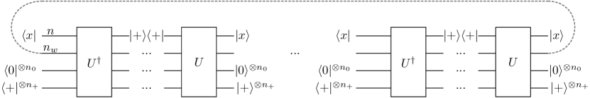
Figure 6: The above figure contains two copies of $M_{x}$. When connecting the right side of the first $M_{x}$ and the left side of the second $M_{x}$, we get the operator $M_{x}^{2}$. Further connecting the left side of the first $M_{x}$ and the right side of the second $M_{x}$ by the dashed line, we get $tr(M_{x}^{2})$.

The proof of Theorem 31 is adapted from the folklore proof of $\mbox{\bf QMA}\subseteq\mbox{\bf PP}$, where the adaption is mainly translating matrix operations (multiplication, trace, etc) to tensor network operations. We only give a proof sketch here.

Proof of Theorem 31.

In this proof we use the notions in Definition 32. Consider a language $L=L_{yes}\cup L_{no}$ in StoqMA with stoquastic verifier $V$ in Definition 32. For input $x$, as pictured in Figure 6 we define a positive semi-definite Hermitian operator acting on $n_{w}$ qubits as

$$M_{x}\coloneqq\langle\phi|U^{\dagger}\Pi_{out}U|\phi\rangle,$$ (143)

where $$|\phi\rangle=\left|x\right\rangle\otimes\left|0\right\rangle^{\otimes n_{0}}\otimes\left|+\right\rangle^{\otimes n_{+}}.$$ (144)

Denote the maximum eigenvalue of $M_{x}$ as $\lambda_{\max}(x)$. By assumption we have that

• If $x\in L_{yes}$, then $\lambda_{\max}(x)\geq b.$

• If $x\in L_{No}$, then $\lambda_{\max}(x)\leq a.$

Since $M_{x}$ is positive semi-definite, then for any $k\in\mathbb{N}$ we have

• If $x\in L_{yes}$, then $tr(M_{x}^{k})\geq b^{k}$.

• If $x\in L_{No}$, then $tr(M_{x}^{k})\leq 2^{n_{w}}a^{k}$.

Recall that $\epsilon\leq 1-\exp(-n)$ is the precision parameter. By the assumption in Theorem 31, there is a $poly(n)$-time randomized algorithm $\mathcal{A}$ such that with probability at least $3/4$, the algorithm returns

$$(1-\epsilon)|\chi(T)|\leq|\hat{\chi}(T)|\leq(1+\epsilon)|\chi(T)|.$$ (145)

To distinguish the yes and no cases, set

$$k\geq\left(n_{w}\ln 2+\ln\frac{1+\epsilon}{1-\epsilon}\right)/\ln\frac{b}{a}=poly(n),$$

We have

$$2^{n_{w}}a^{k}(1+\epsilon)<b^{k}(1-\epsilon).$$ (146)

Thus one can distinguish whether $x\in L_{yes}$ or $x\in L_{no}$ by approximating $tr(M_{x}^{k})$ using the algorithm $\mathcal{A}$.

It remains to explain that $tr(M_{x}^{k})$ can be represented by a positive tensor network $T=T(G,M)$ with $poly(n)$ bond dimension, where $G$ is a $poly(n)$-vertex graph of constant degree.

First notice that similarly as Section C or Section 4.2 in [AL10], one can naturally represent $M_{x}$ as a tensor network $T=T(G,M)$ with $poly(n)$ bond dimension. Since the gates in $U$ are $\rm{X}$, $\rm{CNOT}$, and $\rm{Toffoli}$, and the ancillas are computational basis or $\left|+\right\rangle$, one can check that $T(G,M)$ is a positive tensor network. Further, since $U$ has $poly(n)$ gates and each gate has constant number of input qubits and output qubits, we have that $G$ is a $poly(n)$-vertex graph of constant degree.

To represent $tr(M_{x}^{k})$ as a tensor network, as in Figure 6, it suffices to additionally notice that

• The tensor network for the operator $M_{x}^{2}$ can be represented by putting $2$ copies of $M_{x}$ in a line, then connecting the right side of the first $M_{x}$ and the left side of the second $M_{x}$, that is contracting the free edges w.r.t register $n_{w}$ for the first and second copy.

• Similarly as explained in Eq. (7) in Section 2, if we further connect the left side of the first $M_{x}$ and the right side of the second $M_{x}$ by the dash line, we get $tr(M_{x}^{2})$.

• The tensor network for the operator $tr(M_{x}^{k})$ can be represented similarly. That is putting $k$ copies of $M_{x}$ in a line, and then contracting the free edges w.r.t register $n_{w}$ sequentially.

∎

7 Acknowledgements

We thank Garnet Chan and Zeph Landau for helpful discussions. Part of this work was conducted while the authors were visiting the Simons Institute for the Theory of Computing during summer 2023 and spring 2024, supported by DOE QSA grant $\#$FP00010905. D.H. acknowledges financial support from the US DoD through a QuICS Hartree fellowship. N.S.  acknowledges financial support by the Austrian Science Fund FWF (Grant DOIs 10.55776/COE1 and 10.55776/F71) and the European Union’s Horizon 2020 research and innovation programme through Grant No. 863476 (ERC-CoG SEQUAM). Jiaqing Jiang is supported by MURI Grant FA9550-18-1-0161 and the IQIM, an NSF Physics Frontiers Center (NSF Grant PHY-1125565). Jielun Chen is supported by the US National Science Foundation under grant CHE-2102505.

Appendix A $\#\mbox{\bf P}$-hardness of exactly contracting random 2D tensor networks

Here we prove that the exact contraction of the random 2D tensor network with a positive mean remains $\#\mbox{\bf P}$-hard.

Firstly we prove some properties of standard Gaussian distribution, while the finite precision Gaussian distribution behaves similarly up to $O(\exp(-n))$ derivation in the error bounds. Recall that we use $X\sim\mathcal{N}_{\mathbb{C}}(\mu,\sigma^{2})$ (or $X\sim\mathcal{N}_{\mathbb{R}}(\mu,\sigma^{2})$) to denote that the random variable $X$ is sampled from the complex (or real) Gaussian distribution with mean $\mu$ and standard derivation $\sigma$. We use $\vec{X}=(X_{1},X_{2},\ldots,X_{m})\sim\prod_{i=1}^{m}\mathcal{N}_{\mathbb{C}}(\mu_{i},\sigma^{2})$ to denote the random variable $\vec{X}$ where each $X_{i}$ is independently sampled from $\mathcal{N}_{\mathbb{C}}(\mu_{i},\sigma^{2})$. When $\mu_{i}=\mu,\forall i$, we abbreviate the notation as $\vec{X}\sim\mathcal{N}_{\mathbb{C}}(\mu,\sigma^{2})^{m}$. For two distribution $\mathcal{D}_{1},\mathcal{D}_{2}$, we use $\|\mathcal{D}_{1}-\mathcal{D}_{2}\|$ to denote the total variation distance.

Lemma 33 (Analogy of Lemma 5 in [HHEG20]).

For $\mu_{i}\in\mathbb{C}$. It holds that

$$\|\mathcal{N}_{\mathbb{C}}(\mu,(1-\epsilon)^{2}\sigma^{2})^{m}-\mathcal{N}_{\mathbb{C}}(\mu,\sigma^{2})^{m}\|\leq 4m\epsilon$$ (147)

$$\|\prod_{i=1}^{m}\mathcal{N}_{\mathbb{C}}(\mu_{i},\sigma^{2})-\mathcal{N}_{\mathbb{C}}(\mu,\sigma^{2})^{m}\|\leq\frac{2}{\sigma}\left(|\mu_{1}-\mu|+\ldots+|\mu_{m}-\mu|\right)$$ (148)

Proof.

Recall that for $\mu\in\mathbb{C}$, we use $\Re(\mu),\Im(\mu)\in\mathbb{R}$ for the real and imaginary part of $\mu$, that is $\mu=\Re(\mu)+\Im(\mu)i$. Besides, $X\sim\mathcal{N}_{\mathbb{C}}(\mu,\sigma^{2})$ iff $\Re(X)\sim\mathcal{N}_{\mathbb{R}}(\Re(\mu),\frac{\sigma^{2}}{2}),\Im(X)\sim\mathcal{N}_{\mathbb{R}}(\Im(\mu),\frac{\sigma^{2}}{2})$. It suffices to notice that

$$\|\prod_{i=1}^{m}\mathcal{N}_{\mathbb{C}}(\mu_{i},\sigma_{i}^{2})^{m}-\mathcal{N}_{\mathbb{C}}(\mu,\sigma^{2})^{m}\|$$ (149)

$$=\frac{1}{2}\int_{(x_{1},\ldots,x_{m})}\left|\prod_{i=1}^{m}\frac{1}{2\pi(\sigma_{i}/\sqrt{2})^{2}}\exp^{-\frac{1}{2}|\frac{x_{i}-\mu_{i}}{\sigma_{i}/\sqrt{2}}|^{2}}-\prod_{i=1}^{m}\frac{1}{2\pi(\sigma/2)^{2}}\exp^{-\frac{1}{2}|\frac{x_{i}-\mu}{\sigma/2}|^{2}}\right|dx_{1}\ldots dx_{m}$$ (150)

$$=\frac{1}{2}\int_{(x_{1},\ldots,x_{m})}\left|\prod_{i=1}^{m}\frac{1}{2\pi(\sigma_{i}/\sqrt{2})^{2}}\exp^{-\frac{1}{2}|\frac{x_{i}-\mu_{i}+\mu}{\sigma_{i}/\sqrt{2}}|^{2}}-\prod_{i=1}^{m}\frac{1}{2\pi(\sigma/2)^{2}}\exp^{-\frac{1}{2}|\frac{x_{i}}{\sigma/2}|^{2}}\right|dx_{1}\ldots dx_{m}$$ (151)

$$=\|\prod_{i=1}^{m}\mathcal{N}_{\mathbb{C}}(\mu_{i}-\mu,\sigma_{i}^{2})^{m}-\mathcal{N}_{\mathbb{C}}(0,\sigma^{2})^{m}\|$$ (152)

Thus by Lemma 5 in [HHEG20], we have

$$\|\mathcal{N}_{\mathbb{C}}(\mu,(1-\epsilon)^{2}\sigma^{2})^{m}-\mathcal{N}_{\mathbb{C}}(\mu,\sigma^{2})^{m}\| =\|\mathcal{N}_{\mathbb{C}}(0,(1-\epsilon)^{2}\sigma^{2})^{m}-\mathcal{N}_{\mathbb{C}}(0,\sigma^{2})^{m}\|$$ (153)

$$\leq 2\times 2m\epsilon$$ (154)

$$\|\prod_{i=1}^{m}\mathcal{N}_{\mathbb{C}}(\mu_{i},\sigma^{2})-\mathcal{N}_{\mathbb{C}}(\mu,\sigma^{2})^{m}\| =\|\prod_{i=1}^{m}\mathcal{N}_{\mathbb{C}}(\mu_{i}-\mu,\sigma^{2})-\mathcal{N}_{\mathbb{C}}(0,\sigma^{2})^{m}\|$$ (155)

$$\leq 2\times\frac{1}{\sigma}\left(|\mu_{1}-\mu|+\ldots+|\mu_{m}-\mu|\right)$$ (156)

where we add a $2\times$ since we are working with $\mathcal{N}_{\mathbb{C}}$ while Lemma 5 in [HHEG20] is with $\mathcal{N}_{\mathbb{R}}$. ∎

Proof of Theorem 25.

The proof follows directly from the proof idea of Theorem 2 in [HHEG20]. Here we only give a proof sketch.

Firstly [HHEG20, SWVC07] showed that one can encode any $n$-variable boolean function $f(x_{1},\ldots,x_{n})$ into a projected entangled-pair states (PEPS) of $poly(n)$ vertices, which describes an un-normalized state $\left|\psi\right\rangle$, such that computing $\langle\psi|\psi\rangle$ exactly is equivalent to computing the value

$$s(f)=|\{x\in\{0,1\}^{n}:f(x)=1\}|,$$

which is $\#\mbox{\bf P}$-complete. One can check that in this case $\langle\psi|\psi\rangle$ equals to the contraction value of a 2D tensor network of $poly(n)$ vertices, where the 2D tensor network has bond dimension $d=O(poly(n))$, and every entry of the tensor network is bounded by a constant. one can further make the underlying 2D lattice for the 2D tensor network to have periodic boundary condition, by adding edges connecting boundaries and slightly modify the tensors near the boundary to make sure the contraction value remains invariant. Denote the final 2D lattice with periodic boundary condition as $G$. Denote the final 2D tensor network which encodes the fixed boolean function $f$ as

$$T\left(G,(P^{[v]})_{v}\right)$$

where $P^{[v]}$ is the tensor on vertex $v$. Note that $P^{[v]}$ has $d^{4}$ entries thus $(P^{[v]})_{v}$ are described by in total $d^{4}\times n$ entries. For convinience, we assign an arbitrary order to those entries and denoted them as $\{p_{i}\}_{i=1}^{d^{4}n}$. Recall that by construction we have $|p_{i}|\leq c$ for constant $c$.

Theorem 25 is proved by an argument of average to worse case reduction via interpolation. Here we define the polynomial for the interpolation. Set

$$\epsilon \coloneqq\min\left\{\frac{1}{4(c+\mu+1)d^{4}n^{3}}\,,\,\frac{1}{2}\right\}.$$ (157)

$$k =poly(n)\text{ be sufficiently large.}$$ (158)

Let $$S=\{t_{i}\}_{i\in[k]} k [0,\epsilon]$$ be the set of equidistant points in . (159)

Recall that $0\leq u\leq poly(n)$ thus $\epsilon=1/poly(n)$.

We randomly sample a 2D $(\mu,n,d)$-Gaussian tensor network $T\left(G,(Q^{[v]})_{v}\right)$. Let $t\in S$, define a new 2D tensor network $T(t)$, where for vertex $v$ the tensor $R(t)^{[v]}$ is defined as

$$R(t)^{[v]}\coloneqq tP^{[v]}+(1-t)Q^{[v]}.$$ (160)

Denote the exact contraction value of $T(t)$ as $q(t)$. Note that $q(t)$ is a degree-$n$ polynomial of $t$. Besides, from construction we know that computing $q(1)$ will solve $\#\mbox{\bf P}$-complete problem.

In the following, we show that if one can compute the exact contraction value of finite precision 2D Gaussian tensor network with high probability, then we can compute $q(1)$ with high probability by interpolation. More specifically, For input $T(t)$, denote the value returned by the algorithm $\mathcal{A}$ in Theorem 25 as $\mathcal{A}(t)$.

($i$) First we prove that since $t$ is small, $\mathcal{A}(t)$ is a good approximation of $q(t)$. Specifically, define

$$\mu_{i}=tp_{i}+(1-t)u.$$ (161)

By Eq. (160), we know that the entries of $\left(R(t)^{[v]}\right)_{v}$ are sampled from distribution

$$\mathcal{D}\coloneqq\prod_{i=1}^{d^{4}n}\overline{\mathcal{N}}_{\mathbb{C}}(\mu_{i},(1-t)^{2}).$$ (162)

Since $\overline{\mathcal{N}}_{\mathbb{C}}$ approximates $\mathcal{N}_{\mathbb{C}}$ within exponential precision, we know that

$$\|\mathcal{D}-\overline{\mathcal{N}}_{\mathbb{C}}(\mu,1)^{d^{4}n}\| \leq O(\exp(-n))+\|\prod_{i=1}^{d^{4}n}\mathcal{N}_{\mathbb{C}}(\mu_{i},(1-t)^{2})-\mathcal{N}_{\mathbb{C}}(\mu,1)^{d^{4}n}\|$$ (163)

where by Lemma 7 we have

$$\|\prod_{i=1}^{d^{4}n}\mathcal{N}_{\mathbb{C}}(\mu_{i},(1-t)^{2})-\mathcal{N}_{\mathbb{C}}(\mu,1)^{d^{4}n}\| \leq\|\prod_{i=1}^{d^{4}n}\mathcal{N}_{\mathbb{C}}(\mu_{i},(1-t)^{2})-\mathcal{N}_{\mathbb{C}}(\mu,(1-t)^{2})^{d^{4}n}\|$$

$$+\|\mathcal{N}_{\mathbb{C}}(\mu,(1-t)^{2})^{d^{4}n}-\mathcal{N}_{\mathbb{C}}(\mu,1)^{d^{4}n}\|$$

$$\leq\frac{2}{(1-t)}\left(|\mu_{1}-\mu|+\ldots|\mu_{d^{4}n}-\mu|\right)+4\cdot d^{4}n\cdot t,$$

$$\leq 4\cdot d^{4}n\cdot(c+\mu)\epsilon+4\cdot d^{4}n\cdot\epsilon,$$ (164)

$$\leq 4\cdot d^{4}n\cdot(c+\mu+1)\epsilon$$

$$\leq\frac{1}{n^{2}}$$ (165)

where Eq. (164) comes from the facts that

$$t\leq\epsilon\leq 1/2,$$ (166)

$$|\mu_{i}-\mu|=|t(p_{i}-\mu)|\leq(c+\mu)\epsilon.$$ (167)

Eqs. (163)(165) together imply

$$\|\mathcal{D}-\overline{\mathcal{N}}_{\mathbb{C}}(\mu,1)^{d^{4}n}\| \leq O(\exp(-n))+\frac{1}{n^{2}}.$$ (168)

In other words, for any $t_{i}\in S$, the distribution of $\left(R(t)^{[v]}\right)_{v}$ is almost the same as the finite precision 2D $(\mu,n,d)$-Gaussian tensor network. Let $n$ and $k=poly(n)$ be sufficiently large. By Eq. (168) and the assumption of the performance of $\mathcal{A}$ we have

$$Pr\left(\mathcal{A}(t_{i})=q(t_{i})\right)\geq\frac{3}{4}+\frac{1}{n}-O(\exp(-n))-\frac{1}{n^{2}}\geq\frac{3}{4}+\frac{1}{n^{2}}.$$ (169)

$$E|\{i:\mathcal{A}(t_{i})=q(t_{i})\}|\geq\left(\frac{3}{4}+\frac{1}{n^{2}}\right)k$$ (170)

where in the second inequality $E$ refers to expectation. By Chernouff bound we know that for sufficiently large $k=poly(n)$,

$$Pr\left(|\{i:\mathcal{A}(t_{i})=q(t_{i})\}|\geq\frac{k+n}{2}\right) \geq 1-\exp(-n).$$ (171)

($ii$) We then use the following theorem to recover the degree $n$ polynomial $q(t)$

Theorem 34 (Berlekamp-Welch [Mov18]).

Let $q$ be a degree-$n$ polynomial over any field $\mathbb{F}$. Suppose we are given $k$ pairs of elements $\{(x_{i},y_{i})\}_{i=1}^{k}$ with all $x_{i}$ distinct, and with the promise that $y_{i}=q(x_{i})$ for at least $\max(n+1,(k+n)/2)$ points. Then, one can recover $q$ exactly in $poly(k,n)$ deterministic time.

In Theorem 34 let

$$x_{i}\coloneqq t_{i},$$ (172)

$$y_{i}\coloneqq\mathcal{A}(t_{i}).$$ (173)

Then by Eq. (171) we can recover $q(t)$ with probability $1-\exp(-n)$ in $poly(n)$-time.

($iii)$ Finally, we have $q(t)$ in hand, which is correct with probability $1-\exp(-n)$. Since $q(t)$ is a degree $n$ polynomial, we can easierly compute $q(1)$, which solves a $\#\mbox{\bf P}$-complete problem.

∎

Appendix B More on Barvinok’s method

Proof of Lemma 11.

The proof uses Jensen’s formula and follows the idea from [EM18]. Let $z_{1},\ldots,z_{j},\ldots$ be the roots of $h_{A}(z)$, Jensen’s formula establishes the connection between the roots in the disk $\mathcal{B}(r)$, and the average of $\ln|h_{A}(z)|$ on the boundary of $\mathcal{B}(r)$:

$$\sum_{|z_{j}|\leq r}\ln\frac{r}{|z_{j}|}+\ln|h_{A}(0)|=E_{\theta}\ln|h_{A}(re^{i\theta})|.$$ (174)

First notice that

$$\sum_{|z_{j}|\leq r}\ln\frac{r}{|z_{j}|} \geq\sum_{|z_{j}|\leq r(1-\lambda)}\ln\frac{r}{|z_{j}|}$$ (175)

$$\geq\sum_{|z_{j}|\leq r(1-\lambda)}\ln\frac{r}{r(1-\lambda)}$$ (176)

$$\geq\lambda\cdot N_{A}(r(1-\lambda)).$$ (177)

where in the last inequality we use $\ln\frac{1}{(1-\lambda)}\geq\lambda$ for $\lambda\leq 1/2$. Thus by Eqs. (177)(174), we have

$$E_{A}\left[N_{A}(r-r\lambda)\right] \leq\frac{1}{\lambda}E_{\theta}E_{A}\ln\frac{|h_{A}(re^{i\theta})|}{|h_{A}(0)|}$$ (178)

$$=\frac{1}{2\lambda}E_{\theta}E_{A}\ln\frac{|h_{A}(re^{i\theta})|^{2}}{|h_{A}(0)|^{2}}$$ (179)

$$\leq\frac{1}{2\lambda}\ln E_{\theta}E_{A}\frac{|h_{A}(re^{i\theta})|^{2}}{|h_{A}(0)|^{2}}.$$ (180)

where the last inequality holds since $\ln$ is a concave function. ∎

Lemma 35 (Derivatives of composite function).

Let $G(z)$ and $\phi(z)$ be two functions satisfying $\phi(0)=0$. Let $m$ be an integer. Suppose the first $m$ derivatives $\{G^{(k)}(0)\}_{k=0}^{m}$ and $\{\phi^{(k)}(0)\}_{k=0}^{m}$ can be computed in time $t(n)$ where $n$ is a parameter. Then the first $m$ derivatives of the composite function $G(\phi(z))$ at $z=0$, denoted as

$$\left\{\frac{\partial^{k}}{\partial z^{k}}G(\phi(z))\Big{|}_{z=0}\right\}_{k=1}^{m}$$

can be computed in time $t(n)+O(m^{4})$.

Proof.

For integer $k$ and $r$, define the Bell polynomial to be

$$B_{k,r}(\phi^{(1)}(z),\phi^{(2)}(z),\ldots,\phi^{(k-r+1)}(z))\\ =\sum\frac{k!}{j_{1}!j_{2}!\ldots j_{k-r+1}!}\left(\frac{\phi^{(1)}(z)}{1!}\right)^{j_{1}}\left(\frac{\phi^{(2)}(z)}{2!}\right)^{j_{2}}\ldots\left(\frac{\phi^{(k)}(z)}{k!}\right)^{j_{k-r+1}}$$ (181)

where the summation is

$$j_{1}+j_{2}+\ldots+j_{k-r+1}=r\text{ and }j_{1}+2j_{2}+\ldots+(k-r+1)j_{k-r+1}=k.$$ (182)

To compute the derivative of the composite function $G(\phi(z))$, we will use the Faa di Bruno’s formula which states that

$$\frac{\partial^{k}}{\partial z^{k}}G(\phi(z))\Big{|}_{z=0} =\sum_{r=1}^{k}G^{(r)}(\phi(0))\cdot B_{k,r}(\phi^{(1)}(0),\phi^{(2)}(0),\ldots,\phi^{(k-r+1)}(0))$$ (183)

$$=\sum_{r=1}^{k}G^{(r)}(0)\cdot B_{k,r}(\phi^{(1)}(0),\phi^{(2)}(0),\ldots,\phi^{(k-r+1)}(0)).$$ (184)

where the notation $G^{(r)}(\phi(0))$ refers to $G^{(r)}(z)|_{z=\phi(0)}$ and the last equality comes from $\phi(0)=0$. For each $B_{k,r}$, we define the corresponding partial ordinary Bell polynomials as

$$\hat{B}_{k,r}(y_{1},\ldots,y_{k-r+1})=\frac{r!}{k!}B_{k,r}(x_{1},\ldots,x_{k-r+1})$$ (185)

where $y_{i}=\frac{x_{i}}{i!}$. They satisfy the recurrence formula

$$\hat{B}_{k,r}(y_{1},\ldots,y_{k-r+1})=\sum_{i=1}^{k-r+1}y_{i}\hat{B}_{k-i,r-1}(y_{1},\ldots,y_{k-r+1-i}).$$ (186)

Then after computing the first $m$ derivatives $\{G^{(k)}(0)\}_{k=0}^{m}$ and $\{\phi^{(k)}(0)\}_{k=0}^{m}$ in time $t(n)$, Algorithm 5 computes $B_{k,r}$ in time $O(k^{2}r)$. It suffices to compute $B_{m,r}$ for $r=1,\ldots,m$ since all lower orders can be computed along the way, which takes total time $O(m^{4})$. Therefore, the first $m$ derivatives of $G(\phi(z))$ at $z=0$ can be computed in time $t(n)+O(m^{4})$.

Algorithm 5 Compute Bell polynomials [Tag23]

1:Set $y_{i}\leftarrow x_{i}/i!$, $i=1,\ldots,k-r+1$

2:Set $\hat{B}_{0,0}=1$, $\hat{B}_{i,0}=0$, $i=1,\ldots,k-r$

3:for $l=1,\ldots,r$ do

4:     for $i=l,\ldots,k-r+l$ do

5:         $\hat{B}_{i,l}(y_{1},\ldots,y_{k-r+1})\leftarrow\sum_{j=1}^{i-l+1}y_{j}\hat{B}_{i-j,l-1}(y_{1},\ldots,y_{k-r+1})$

6:     end for

7:end for

8:Set $B_{k,r}(x_{1},\ldots,x_{k-r+1})\leftarrow\frac{k!}{r!}\hat{B}_{k,r}(y_{1},\ldots,y_{k-r+1})$

∎

Appendix C BPP-hardness of additive-error approximation (Theorem 27)

In this section, we prove the approximation problem in Theorem 27 is BPP-hard. This proof is similar to Section 4.2 in [AL10] and here we give a proof sketch.

First we embed classical randomized computations into quantum circuits. Given a parameter $n$, consider a quantum circuit of following form:

• Takes input as $\left|0\right\rangle^{p}\left|+\right\rangle^{q}$ for $p,q=poly(n)$.

• Applies a sequence of gates $Q=Q_{L}\ldots Q_{1}$, where $L=poly(n)$ and $\{Q_{i}\}_{i}$ are reversible gates on constant qubits.

• Measure the first qubit in computational basis.

Denote $p_{0}$ as the probability of getting measurement outcome $0$ in the first qubit. Suppose it is promised that either one of the following holds:

• Yes case: $p_{0}\geq 2/3$

• No case: $p_{0}\leq 1/3$.

One can check that the problem of given such a circuit, output Yes/No correctly with probability greater than $2/3$ is BPP-hard. In other word

Claim 36.

An algorithm for estimating $p_{0}$ with high probability is BPP-hard.

Similarly as [AL10], to write $p_{0}$ as a tensor network, we first define a related circuit $U$ on $p+q+1$ qubits: As shown in Figure 7, U firstly applies $Q$ to $|0^{\otimes(p+1)},+^{\otimes q}\rangle$, then copies the first qubit of $Q$ to the additional qubit by CNOT, and then applies $Q^{-1}$.

Figure 7: Circuit for $p_{0}$

One can check that

$$\langle 0^{\otimes(p+1)},+^{\otimes q}\big{|}U\big{|}0^{\otimes(p+1)},+^{\otimes q}\rangle=p_{0}.$$

One can transform $\langle 0^{\otimes(p+1)},+^{\otimes q}\big{|}U\big{|}0^{\otimes(p+1)},+^{\otimes q}\rangle$ to a tensor network $T$ similarly as [AL10], then

$$\chi(T)=\langle 0^{\otimes(p+1)},+^{\otimes q}\big{|}U\big{|}0^{\otimes(p+1)},+^{\otimes q}\rangle=p_{0},$$ (187)

where

• Each reversible gate $Q_{i}$ on constant qubits is translated to a tensor $M^{[Q_{i}]}$, which is of constant rank (constant degree) and bond dimension $2$. Note that since $Q_{i}$ is a reversible gate, which is a permutation, thus we have $\|Q_{i}\|_{1}=1$.

• We pair the input qubits on the left and right in Figure 7. $|0\rangle\langle 0|$ is translated into a tensor $M^{[0]}=\begin{bmatrix}1&0\\ 0&0\end{bmatrix}$, $|+\rangle\langle+|$ is translated into a tensor $M^{[+]}=\frac{1}{2}\begin{bmatrix}1&1\\ 1&1\end{bmatrix}$. Note that $\|M^{[0]}\|_{1}=\|M^{[+]}\|_{1}=1$.

Thus the approximation scale $\Delta_{1}$ in Eq. (121) is equal to $1$. Thus for $\epsilon=1/poly(n)$, the approximation problem in Theorem 27, that is Eq. (120), requires approximating $\chi(T)=p_{0}$ within precision $\epsilon$ with high probability, thus is BPP-hard by Claim 36.

References

- [AB09] Sanjeev Arora and Boaz Barak. Computational complexity: a modern approach. Cambridge University Press, 2009.
- [AL10] Itai Arad and Zeph Landau. Quantum computation and the evaluation of tensor networks. SIAM Journal on Computing, 39(7):3089–3121, 2010.
- [ALVV17] Itai Arad, Zeph Landau, Umesh Vazirani, and Thomas Vidick. Rigorous rg algorithms and area laws for low energy eigenstates in 1d. Communications in Mathematical Physics, 356:65–105, 2017.
- [Ban23] Mari Carmen Banuls. Tensor network algorithms: A route map. Annual Review of Condensed Matter Physics, 14(1):173–191, March 2023.
- [Bar14] Alexander Barvinok. Computing the partition function for cliques in a graph. arXiv preprint arXiv:1405.1974, 2014.
- [Bar16a] Alexander Barvinok. Approximating permanents and hafnians. arXiv preprint arXiv:1601.07518, 2016.
- [Bar16b] Alexander Barvinok. Computing the permanent of (some) complex matrices. Foundations of Computational Mathematics, 16:329–342, 2016.
- [BBA21] Yimu Bao, Maxwell Block, and Ehud Altman. Finite time teleportation phase transition in random quantum circuits. arXiv preprint arXiv:2110.06963, 2021.
- [BBT06] Sergey Bravyi, Arvid J Bessen, and Barbara M Terhal. Merlin-arthur games and stoquastic complexity. arXiv preprint quant-ph/0611021, 2006.
- [BCA20] Yimu Bao, Soonwon Choi, and Ehud Altman. Theory of the phase transition in random unitary circuits with measurements. Physical Review B, 101(10):104301, 2020.
- [BSV14] Sergey Bravyi, Martin Suchara, and Alexander Vargo. Efficient algorithms for maximum likelihood decoding in the surface code. Physical Review A, 90(3):032326, 2014.
- [CJHS24] Jielun Chen, Jiaqing Jiang, Dominik Hangleiter, and Norbert Schuch. Sign problem in tensor network contraction. arXiv preprint arXiv:2404.19023, 2024.
- [Cor16] Philippe Corboz. Variational optimization with infinite projected entangled-pair states. Physical Review B, 94(3):035133, 2016.
- [EM18] Lior Eldar and Saeed Mehraban. Approximating the permanent of a random matrix with vanishing mean. In 2018 IEEE 59th Annual Symposium on Foundations of Computer Science (FOCS), pages 23–34. IEEE, 2018.
- [EV15] Glen Evenbly and Guifre Vidal. Tensor network renormalization. Physical review letters, 115(18):180405, 2015.
- [FP14] Andrew J Ferris and David Poulin. Tensor networks and quantum error correction. Physical review letters, 113(3):030501, 2014.
- [GC22] Johnnie Gray and Garnet Kin-Lic Chan. Hyper-optimized compressed contraction of tensor networks with arbitrary geometry. arXiv preprint arXiv:2206.07044, 2022.
- [GLX+19] Chu Guo, Yong Liu, Min Xiong, Shichuan Xue, Xiang Fu, Anqi Huang, Xiaogang Qiang, Ping Xu, Junhua Liu, Shenggen Zheng, et al. General-purpose quantum circuit simulator with projected entangled-pair states and the quantum supremacy frontier. Physical review letters, 123(19):190501, 2019.
- [Has07] Matthew B Hastings. An area law for one-dimensional quantum systems. Journal of statistical mechanics: theory and experiment, 2007(08):P08024, 2007.
- [HHEG20] Jonas Haferkamp, Dominik Hangleiter, Jens Eisert, and Marek Gluza. Contracting projected entangled pair states is average-case hard. Physical Review Research, 2(1):013010, 2020.
- [HNQ+16] Patrick Hayden, Sepehr Nezami, Xiao-Liang Qi, Nathaniel Thomas, Michael Walter, and Zhao Yang. Holographic duality from random tensor networks. Journal of High Energy Physics, 2016(11):1–56, 2016.
- [HPR19] Tyler Helmuth, Will Perkins, and Guus Regts. Algorithmic pirogov-sinai theory. In Proceedings of the 51st Annual ACM SIGACT Symposium on Theory of Computing, pages 1009–1020, 2019.
- [HZN+20] Cupjin Huang, Fang Zhang, Michael Newman, Junjie Cai, Xun Gao, Zhengxiong Tian, Junyin Wu, Haihong Xu, Huanjun Yu, Bo Yuan, et al. Classical simulation of quantum supremacy circuits. arXiv preprint arXiv:2005.06787, 2020.
- [Kau49] Bruria Kaufman. Crystal statistics. ii. partition function evaluated by spinor analysis. Physical Review, 76(8):1232, 1949.
- [LC21] Ryan Levy and Bryan K Clark. Entanglement entropy transitions with random tensor networks. arXiv preprint arXiv:2108.02225, 2021.
- [Maj66] Chanchal K Majumdar. Analytic properties of the onsager solution of the ising model. Physical Review, 145(1):158, 1966.
- [MH21] Ryan L Mann and Tyler Helmuth. Efficient algorithms for approximating quantum partition functions. Journal of Mathematical Physics, 62(2), 2021.
- [Mov18] Ramis Movassagh. Efficient unitary paths and quantum computational supremacy: A proof of average-case hardness of random circuit sampling. arXiv preprint arXiv:1810.04681, 2018.
- [MS08] Igor L Markov and Yaoyun Shi. Simulating quantum computation by contracting tensor networks. SIAM Journal on Computing, 38(3):963–981, 2008.
- [MVC07] Valentin Murg, Frank Verstraete, and J Ignacio Cirac. Variational study of hard-core bosons in a two-dimensional optical lattice using projected entangled pair states. Physical Review A, 75(3):033605, 2007.
- [Ons44] Lars Onsager. Crystal statistics. i. a two-dimensional model with an order-disorder transition. Physical Review, 65(3-4):117, 1944.
- [Orú19] Román Orús. Tensor networks for complex quantum systems. Nature Reviews Physics, 1(9):538–550, 2019.
- [PGN+17] Edwin Pednault, John A Gunnels, Giacomo Nannicini, Lior Horesh, Thomas Magerlein, Edgar Solomonik, and Robert Wisnieff. Breaking the 49-qubit barrier in the simulation of quantum circuits. arXiv preprint arXiv:1710.05867, 15, 2017.
- [PR17] Viresh Patel and Guus Regts. Deterministic polynomial-time approximation algorithms for partition functions and graph polynomials. SIAM Journal on Computing, 46(6):1893–1919, 2017.
- [SBE17] Martin Schwarz, Olivier Buerschaper, and Jens Eisert. Approximating local observables on projected entangled pair states. Physical Review A, 95(6):060102, 2017.
- [SRN19] Brian Skinner, Jonathan Ruhman, and Adam Nahum. Measurement-induced phase transitions in the dynamics of entanglement. Physical Review X, 9(3):031009, 2019.
- [SWVC07] Norbert Schuch, Michael M Wolf, Frank Verstraete, and J Ignacio Cirac. Computational complexity of projected entangled pair states. Physical review letters, 98(14):140506, 2007.
- [Tag23] Hamed Taghavian. A fast algorithm for computing bell polynomials based on index break-downs using prime factorization, 2023.
- [VC21] Patrick CG Vlaar and Philippe Corboz. Simulation of three-dimensional quantum systems with projected entangled-pair states. Physical Review B, 103(20):205137, 2021.
- [VHCV16] Laurens Vanderstraeten, Jutho Haegeman, Philippe Corboz, and Frank Verstraete. Gradient methods for variational optimization of projected entangled-pair states. Physical Review B, 94(15):155123, 2016.
- [Whi92] Steven R White. Density matrix formulation for quantum renormalization groups. Physical review letters, 69(19):2863, 1992.
- [Whi93] Steven R White. Density-matrix algorithms for quantum renormalization groups. Physical review b, 48(14):10345, 1993.
- [YLFC22] Zhi-Cheng Yang, Yaodong Li, Matthew PA Fisher, and Xiao Chen. Entanglement phase transitions in random stabilizer tensor networks. Physical Review B, 105(10):104306, 2022.
- [ZXC+10] Hui-Hai Zhao, Zhi-Yuan Xie, Qihong N Chen, Zhong-Chao Wei, Jianwei W Cai, and Tao Xiang. Renormalization of tensor-network states. Physical Review B, 81(17):174411, 2010.