A long spin period for a sub-Neptune-mass exoplanet

Abstract

HIP 41378 f is a sub-Neptune exoplanet with an anomalously low density. Its long orbital period and deep transit make it an ideal candidate for detecting oblateness photometrically. We present a new cross-platform, GPU-enabled code greenlantern, suitable for computing transit light curves of oblate planets at arbitrary orientations. We then use Markov Chain Monte Carlo to fit K2 data of HIP 41378 b, d, and f, specifically examining HIP 41378 f for possible oblateness and obliquity. We find that the flattening of HIP 41378 f is $f\leq 0.18$ at the 95% confidence level, consistent with a rotation period of $P_{\text{rot}}\geq 22.2$ hr. In the future, high-precision data from JWST has the potential to tighten such a constraint and can differentiate between spherical and flattened planets.

1 Introduction

The distribution of angular momentum within a planetary system, including both orbital and rotational angular momentum for each body, serves as a valuable dynamical tracer, helping us to constrain the formation and evolution of the system. One of the most challenging measurements to obtain is the rotational angular momentum of a planet. The magnitude of the angular momentum is set by physical planet parameters (the planetary mass, radius, and interior density profile), which are largely fixed at formation, and the planetary rotation rate, while may evolve due to dynamical interactions post-formation. The direction of the angular momentum, referred to as the planetary obliquity, also provides insight into the planet’s formation and subsequent dynamical evolution (e.g., Slattery et al., 1992; Laskar & Robutel, 1993; Millholland et al., 2024).

The non-sphericity of a planetary body can also be used to infer its rotational angular momentum. Planets with short rotational periods may become oblate due to rapid rotation, with faster rotators experiencing greater deformation (Seager & Hui, 2002). At the same time, the planet’s obliquity determines how the planet’s rotational axis is oriented relative to the observer’s line of sight. For directly imaged planets, a planet’s rotation can be measured through direct spectroscopy (e.g., Bryan et al., 2020, 2021). For planets seen in transit, the resulting light curve of a oblate body will reflect a flattened shape, rather than the commonly assumed spherical transiting body. This shape is often parameterized in terms of a flattening $f$, as in Barnes & Fortney (2003):

$$f\equiv\frac{R_{\text{eq}}-R_{\text{pol}}}{R_{\text{eq}}},$$ (1)

where $R_{\text{eq}}$ is the planet’s equatorial radius and $R_{\text{pol}}$ is its polar radius. Barnes & Fortney (2003) present a case study on HD 209458 b, demonstrating that planetary oblateness introduces a deviation from the spherical light curve. While this deviation is small — about 10 ppm — it can bias the accurate recovery of other transit parameters if flattening is not accounted for in the fits (Berardo & de Wit, 2022). Precise instrumentation, long observation baselines, and appropriate oblate transit models allow the possibility of detecting such a signal and subsequently constraining planetary oblateness and obliquity. However, due to the difficulty of the measurement of such a small signal, only a few detections and constraints of such deformation have been made to date, and only for Jupiter-sized planets where the signal is more pronounced (Zhu et al., 2014; Biersteker & Schlichting, 2017).

The transit fits used in the vast majority of planet discovery and characterization papers assume spherical bodies, since computing a light curve using a non-spherical model is significantly more computationally expensive. Despite this computational limitation, there have been previous efforts to build codes to model the transit of an ellipsoidal body. Initial work by Barnes & Fortney (2003) use a numerical integration scheme based on Romberg’s method to compute the fraction of light blocked by an orbiting ellipse, weighted by the stellar intensity. This approach effectively requires two levels of integration, which is less efficient than the approach taken by Pál (2012) for spherical planets, which leverages Green’s theorem to reduce the dimensionality of the integral. Other works, such as Carter & Winn (2010), Carado & Knuth (2020), and Berardo & de Wit (2022) use Monte Carlo integration to evaluate the area of the projected ellipsoid that lies within the stellar disk. Leconte et al. (2011) consider phase curves of ellipsoid bodies, but that approach cannot be directly applied to transit light curves: For the phase curve, only the projected area is needed, but transit modeling requires the functional form of the boundary to handle its intersection with the stellar disk during transit.

In this work, we present a publicly-available, GPU-accelerated, and cross-platform code greenlantern, which combines the advantages of the Pál (2012) methodology with ellipsoid planet geometry to compute transit light curves of ellipsoids at any orientation. This code will allow for more efficient calculation of ellipsoidal transit models. We demonstrate its functionality by applying our new code to the light curve of HIP 41378 f, a cold sub-Neptune, and constraining its rotation rate. HIP 41378 f in an excellent target for such a constraint due to its large radius, bright host star, and low bulk density. At the same time, HIP 41378 f is a planet were a rotation rate would provide significant dynamical insight: formation models remain uncertain on how to explain the low bulk density (Santerne et al., 2019) and low inferred core mass (Belkovski et al., 2022) of such a cold, Jupiter-radius planet. These investigations would be aided by a constraint on HIP 41378 f’s rotation.

This paper is structured as follows. In Section 2, we present our analytic model for the projected profile of a triaxial ellipsoid and the computational method that computes the associated transit light curve. In Section 3, we present the dataset for HIP 41378 and our method for fitting the model to this data. Section 4 describes the constraints we derive on the flattening and obliquity of HIP 41378, and the implications of our findings are discussed in Section 5. Finally, we conclude in Section 6.

2 Ellipsoid transit model

We work in a Cartesian coordinate system where the $\hat{\bm{z}}$ axis points along the line of sight from the observer to the host star. The $\hat{\bm{y}}$ axis is oriented along the “horizontal” transit chord, and the $\hat{\bm{x}}$ axis is oriented in the remaining perpendicular direction, so that the resulting coordinate system is right-handed. We choose three rotation angles $\alpha$, $\beta$, and $\gamma$ that rotate the ellipsoid around $\hat{\bm{x}}$, $\hat{\bm{y}}$, and $\hat{\bm{z}}$, respectively, and an offset distance $d_{\star}$ from the center of the host star. The coordinate system and three rotations are shown in Figure 1. In these coordinates, $\alpha$ plays the role of the mean anomaly of the orbit (assuming zero eccentricity) where $\alpha=0^{\circ}$ is midtransit; $\beta$ is an elevation angle, such that $\beta=90^{\circ}-i$ relates $\beta$ and the traditional inclination angle $i$; and $\gamma$ sets the obliquity.

Figure 1: Illustration of the coordinate system and rotation angles used to model the transit of an ellipsoidal planet. The observer’s line of sight aligns with the $\hat{\bm{z}}$ axis and the $\hat{\bm{y}}$ axis is oriented along the horizontal transit chord; the $\hat{\bm{x}}$ axis is mutually perpendicular to $\hat{\bm{y}}$ and $\hat{\bm{z}}$ such that the coordinate system follows the right-hand rule. The ellipsoidal planet’s geometry is described by three rotation angles: $\alpha$ (rotation around $\hat{\bm{x}}$), $\beta$ (rotation around $\hat{\bm{y}}$), and $\gamma$ (rotation around $\hat{\bm{z}}$), which correspond to the mean anomaly, the elevation angle $\beta=90^{\circ}-i$, and the planetary obliquity, respectively. The orbital distance $d_{\star}$ is measured to the stellar center; though the star is spherical by assumption, we collapse its geometry to a plane for simplicity. The left panel shows the rotation of the ellipsoid by $\alpha$, the middle panel illustrates rotation by $\beta$, and the right panel depicts rotation by $\gamma$.

We additionally define a set of primed coordinates, $\hat{\bm{x}}^{\prime}$, $\hat{\bm{y}}^{\prime}$, and $\hat{\bm{z}}^{\prime}$, along the three semiaxes of the ellipsoid, which have lengths $a$, $b$, and $c$, respectively. Then, the angles and offset we have defined relate the two coordinate systems though a series of three rotations: first in $\alpha$, then in $\beta$, and finally in $\gamma$.

Computing the projection of an ellipsoid onto the $x$–$y$ plane can be done with a computer algebra system, though simplifying the resulting expressions into a compact and usable form is tedious. Here, we present one such simplification. We define the following four quantities which are dimensionless functions of $\alpha$, $\beta$, and $\gamma$,

$$q \equiv\cos{\beta}\cos{\gamma}-\sin{\alpha}\sin{\beta}\sin{\gamma}$$ (2)

$$u \equiv\sin{\alpha}\sin{\beta}\cos{\gamma}+\cos{\beta}\sin{\gamma}$$ (3)

$$r \equiv\sin{\beta}\cos{\gamma}+\sin{\alpha}\cos{\beta}\sin{\gamma}$$ (4)

$$s \equiv\sin{\alpha}\cos{\beta}\cos{\gamma}-\sin{\beta}\sin{\gamma}.$$ (5)

Solving for the bounding curve of the ellipsoid projection, we find the parametric representation

$$x_{\text{e}} =x_{0}+\delta x\cos{\theta}$$ (6)

$$y_{\text{e}} =y_{0}+\delta y_{1}\cos{\theta}+\delta y_{2}\sin{\theta}$$ (7)

in terms of an angle $\theta$, where

$$x_{0}=-d_{\star}\cos{\alpha}\sin{\beta},$$ (8)

$$\delta x=\sqrt{b^{2}+q^{2}\left(a^{2}-b^{2}\right)-\left(b^{2}-c^{2}\right)\cos^{2}{\alpha}\sin^{2}{\beta}},$$ (9)

$$y_{0}=d_{\star}\sin{\alpha}\left[a^{2}-\left(a^{2}-c^{2}\right)\cos^{2}{\alpha}\sin^{2}{\beta}-u^{2}\left(a^{2}-b^{2}\right)\right]\Big{/}\delta x^{2},$$ (10)

$$\delta y_{1}=\cos{\alpha}\left[\left(a^{2}-c^{2}\right)\sin{\alpha}\sin{\beta}-u\left(a^{2}-b^{2}\right)\cos{\gamma}\right]\Big{/}\delta x,$$ (11)

$$\delta y_{2}=\sqrt{a^{2}b^{2}\cos^{2}{\alpha}\cos^{2}{\beta}+b^{2}c^{2}r^{2}+a^{2}c^{2}s^{2}}\Big{/}\delta x.$$ (12)

We follow the approach of Pál (2012) in leveraging Green’s theorem to convert an integral over area within this closed curve into a line integral, which we parameterize by $\theta$; this approach also allows us to account for the effects of stellar limb darkening. We require the quantities

$$\frac{\partial x_{\text{e}}}{\partial\theta} =-\delta x\sin{\theta}$$ (13)

$$\frac{\partial y_{\text{e}}}{\partial\theta} =-\delta y_{1}\sin{\theta}+\delta y_{2}\cos{\theta}$$ (14)

to compute the line integrals.

We have not yet addressed how to handle the case when the bounding curve intersects — or falls completely outside — the stellar disk, however, and this becomes important for evaluating these line integrals, since the desired area is the intersection of the stellar disk with the boundary of the projected ellipsoid. Solving for the points of intersection of the projected ellipsoid curve with the stellar disk, assumed to be a circle of unit radius, is unnecessary and actually detrimental to the accurate and efficient evaluation of the line integral. Instead, if a point on the projected ellipsoid curve $\left(x_{\text{e}},y_{\text{e}}\right)$ falls outside the stellar disk, $x_{\text{e}}^{2}+y_{\text{e}}^{2}>1$, we “snap” the coordinate to the coordinate along the same ray from the center of the stellar disk that falls on the edge of the stellar disk, $\left(x_{\text{d}},y_{\text{d}}\right)$; this is illustrated in Figure 2. We compute an angle $\xi$ such that

$$\xi\equiv\tan^{-1}{y_{\text{e}}/x_{\text{e}}}$$ (15)

and then have

$$x_{\text{d}} =\cos{\xi}, y_{\text{d}} =\sin{\xi},$$ (16)

$$\frac{\partial x_{\text{d}}}{\partial\theta} =-y_{\text{d}}\frac{\partial\xi}{\partial\theta}, \frac{\partial y_{\text{d}}}{\partial\theta} =x_{\text{d}}\frac{\partial\xi}{\partial\theta},$$ (17)

where

$$\frac{\partial\xi}{\partial\theta}=\left(-y_{\text{e}}\frac{\partial x_{\text{e}}}{\partial\theta}+x_{\text{e}}\frac{\partial y_{\text{e}}}{\partial\theta}\right)\Big{/}\left(x_{\text{e}}^{2}+y_{\text{e}}^{2}\right).$$ (18)

When this point $\left(x_{\text{d}},y_{\text{d}}\right)$ is used instead of $\left(x_{\text{e}},y_{\text{e}}\right)$, we can rewrite the line integral, now parameterized by $\xi$, to parameterize by $\theta$ again, since

$$\oint\limits_{\text{d}}f\!\left(x,y\right)\mathop{}\!\mathup{d}\xi=\oint\limits_{\text{d}}f\!\left(x,y\right)\frac{\partial\xi}{\partial\theta}\mathop{}\!\mathup{d}\theta.$$ (19)

Figure 2: Diagram of the coordinate “snapping” described in the text. The point $\left(x_{\text{e}},y_{\text{e}}\right)$ on the boundary of the projected ellipsoid falls outside the stellar disk, so the line integral should be carried out on the dashed purple curve instead of the solid purple curve. This point can be mapped to the point on the disk edge at the same angular displacement $\xi$, $\left(x_{\text{d}},y_{\text{d}}\right)$.

For a quadratic stellar limb darkening model, we need to evaluate the integrals of three functions, derived by Pál (2012),

$$f_{\text{flat}} =\frac{1}{2}\left(x\frac{\partial y}{\partial\theta}-y\frac{\partial x}{\partial\theta}\right),$$ (20)

$$f_{\text{lin}} =\frac{2}{3}\left[1-\left(1-x^{2}-y^{2}\right)^{3/2}\right]f_{\text{flat}}\Big{/}\left(x^{2}+y^{2}\right),$$ (21)

$$f_{\text{quad}} =\frac{1}{2}\left[x\left(\frac{x^{2}}{3}+y^{2}\right)\frac{\partial y}{\partial\theta}-y\left(x^{2}+\frac{y^{2}}{3}\right)\frac{\partial x}{\partial\theta}\right],$$ (22)

over the closed curve encompassing the area of the projected ellipsoid that is also within the stellar disk. In these integrands, $\left(x,y\right)$ are either $\left(x_{\text{e}},y_{\text{e}}\right)$ when $x_{\text{e}}^{2}+y_{\text{e}}^{2}<1$ or $\left(x_{\text{d}},y_{\text{d}}\right)$ when $x_{\text{e}}^{2}+y_{\text{e}}^{2}>1$. Computationally, the latter case depends on quantities computed for the former, so only one branching instruction is needed to modify the values used in evaluating this integrand. The final value of each integral is computed numerically using Simpson’s rule.

Minimizing branching this way allows us to leverage the massive parallelization available on graphics processing units (GPUs), and each sum can be computed efficiently using hierarchical parallelism on GPU. Solving for the intersections of the ellipsoid projection with the stellar disk, as done by Liu et al. (2024a), introduces so much additional branching that we observed degraded performance with that approach on GPU, in addition to numerical instability if roots were not found to high enough precision. We use single precision floating point, along with a few measures for mitigating numerical noise, since these can have better than twice the efficiency of double precision floating point on GPUs. For example, the NVIDIA Quadro RTX 5000 card used in our calculations has a peak 32-to-1 performance ratio favoring single precision over double precision.

2.1 Model validation

A first test to demonstrate the accuracy of our method and implementation is comparing the flux predicted by our model for a spherical shape, where the semi-axis lengths of the ellipsoid $a=b=c$, to that of an established code, batman (Kreidberg, 2015). In Figure 3, we provide several example light curves computed with both codes and the residuals between them, showing good qualitative and quantitative agreement at sub-ppm levels. Some noise is expected since our code computes in single precision floating point, but the amplitude does not exceed 0.5 ppm in any of the demonstrations.

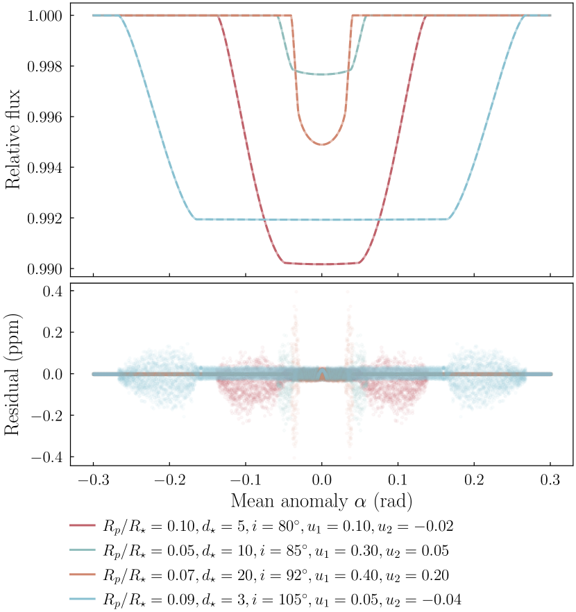
Figure 3: Gallery of several validation tests performed against batman (Kreidberg, 2015) showing the computed light curve (top panel) and absolute residual (bottom panel); the parameters for each test are given in the key below the plot. In the top panel, the light, solid curves are output from batman, and the dark, dashed curves are output from greenlantern, showing qualitative and quantitative agreement. The maximum absolute residual is encountered during ingress and egress and does not exceed 0.5 ppm.

Barnes & Fortney (2003) simulate the flux of HD 209458b as if it were oblate with flattening parameter $f=0.1$. Since they explore the dependence on a variety of transit parameters, and because they use a different method than this work, their results serve as a useful benchmark for ours. In Figures 4 and 5, we reproduce Barnes & Fortney (2003) Figures 4 and 9, respectively, showing strong qualitative agreement with their findings.

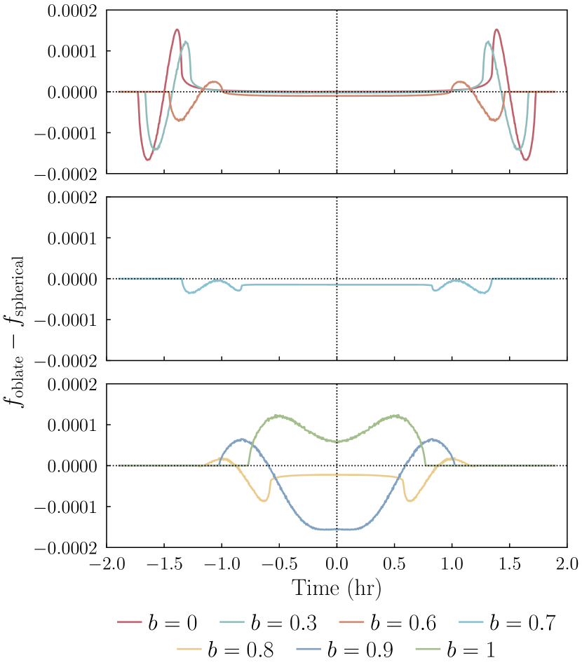
Figure 4: Analog to Figure 4 of Barnes & Fortney (2003), showing the difference between the relative flux of an oblate transit model and the spherical counterpart of the same cross-sectional area at mid-transit and $b=0$, for various values of impact parameter $b$. The small-amplitude numerical noise visible in the plot is expected since the computations are carried out in single precision floating point.

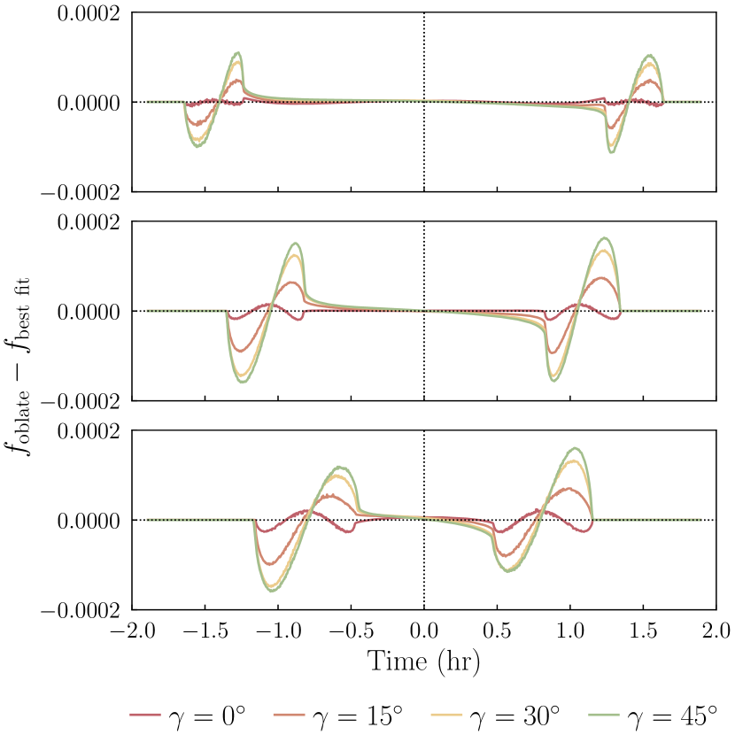
Figure 5: Analog to Figure 9 of Barnes & Fortney (2003), showing the difference between the relative flux of an oblate transit model and the best fit spherical model, for various values of obliquity angle $\gamma$ and impact parameter $b$. The small-amplitude numerical noise visible in the plot is expected since the computations are carried out in single precision floating point. Note that this figure is a mirror image of its counterpart because of the way we define the angle $\gamma$.

2.2 Code performance

The batman code for spherical planet transits (Kreidberg, 2015) also provides a useful benchmark to demonstrate the speed of our approach. In Figure 6, we show the wall time per flux sample for both codes, averaged over ten trials, for a variety of workload sizes. When only a few hundred points are computed, greenlantern is about half as fast as batman, but, as the workload increases to tens or hundreds of thousands of points, we asymptotically approach a comparable timing of about 0.5 µs per sample. Since greenlantern offers additional functionality over batman — the ability to compute general triaxial ellipsoid transits — some computational cost is expected, but we show that it is not unreasonable.

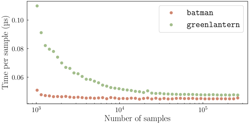
Figure 6: Performance of the code presented in this work, greenlantern, compared to the popular spherical transit modeling code batman (Kreidberg, 2015). By running on GPU, our code achieves similar timings per sample once at least $10^{4}$ samples are computed. The maximum absolute error compared to batman across all trials was $1.33\times 10^{-7}$, close to machine epsilon for single precision floating point.

3 Data and model fitting

We apply our newly-developed code to the HIP 41378 system, which consists of at least five known planets, including a particularly intriguing cold puffy sub-Neptune-mass planet, HIP 41378 f (Vanderburg et al., 2016a; Santerne et al., 2019). HIP 41378 f has an extremely low measured bulk density (0.09 g/cm³; Santerne et al., 2019; Harada et al., 2023) and a cold orbit far from its host star (Becker et al. 2019; Berardo et al. 2019; orbital period 542.08 days, Santerne et al. 2019). Previous observations with the Hubble Space Telescope have found a flat transmission spectrum shape for HIP 41378 f (Alam et al., 2022).

HIP 41378 was observed during K2’s Campaign 5 in long-cadence mode, and during Campaign 18 in short-cadence mode. Utilizing greenlantern, we fit the K2 light curve data to derive a constraint on HIP 41378 f’s rotation rate. We used the K2 observations as reduced by Vanderburg et al. (2016a) and Becker et al. (2019). In brief, these light curves were extracted from target pixel files from a set of 20 photometric apertures and systematics corrections were performed following Vanderburg & Johnson (2014) and Vanderburg et al. (2016b). After selecting the light curve from the aperture that minimized photometric scatter, the systematics correction was refined by a simultaneous fit along with the transits and low-frequency variability in the light curve. We flattened the light curve by dividing the resulting light curve by the best-fit low-frequency variability model. The original target pixel files for K2 Campaigns 5 and 18 are hosted by MAST: 10.17909/T9SK5H (catalog 10.17909/T9SK5H) and 10.17909/t9-zmte-d528 (catalog 10.17909/t9-zmte-d528), respectively.

We manually separate non-overlapping transits of planets b, d, and f in preprocessing and fit each model to the appropriate data (planet b parameters to transits of planet b, etc.). This is done to mitigate possible model confusion, since a combined model could swap the parameters of two planets and produce the same likelihood. Splitting the data in preprocessing removes this degeneracy so that MCMC walkers do not explore unnecessary areas of parameter space.

The full model consists of 26 parameters. Five parameters are needed for each of planets b and d: the radius ratio $R_{p}/R_{\star}$, orbital period $P_{\text{orb}}$, orbital distance during transit $d/R_{\star}$, mid-transit time offset $t_{0}$, and complement inclination angle $\beta$. For planet f, which we examine for possible oblateness and obliquity, we require eight parameters: the polar ($R_{a}/R_{\star}$) and equatorial ($R_{bc}/R_{\star}$) radius ratios, orbital period $P_{\text{orb}}$, orbital distance during transit $d/R_{\star}$, mid-transit time offset $t_{0}$, complement inclination angle $\beta$, and obliquity angle parameters $\Gamma\cos\gamma$ and $\Gamma\sin\gamma$. Common to all three planets modeled are the stellar limb darkening parameters $q_{1},q_{2}$, following the parameterization of Kipping (2013).

Fitting for three orbital periods and three orbital distances, given that the stellar density $\rho_{\star}$ is constrained independently by asteroseismology (Lund et al., 2019), allows us to efficiently approximate a possibly nonzero orbital eccentricity for each planet. Orbital period $P_{\text{orb}}$ and $\rho_{\star}$ uniquely set the semimajor axis $a/R_{\star}$ for each planet; so we distinguish the orbital distance during transit with the symbol $d/R_{\star}$, which is equivalent to $a/R_{\star}$ when eccentricity $e=0$. This is an approximation based on the assumption that $d/R_{\star}$ remains constant throughout the transit, rather than varying with time. We expect eccentricity to be small if it is nonzero, so the value of $a/R_{\star}$ for each planet is used to set the prior on $d/R_{\star}$.

Our parameterization of obliquity as two parameters, $\Gamma\cos\gamma$ and $\Gamma\sin\gamma$, also deserves additional explanation. Because the obliquity angle $\gamma$ we use is periodic, an unbounded Monte Carlo exploration of this parameter space cannot truly converge, and bounding the range of $\gamma$ could bias its posterior (e.g., Eastman, 2024). Inspired by the creative solution of Eastman (2024) for fitting the argument of periastron of eccentric orbits, we reparameterize $\gamma$ similarly, defining a nuisance parameter $\Gamma$ that is arbitrarily, but conveniently, bounded such that $\lvert\Gamma\rvert\leq 1$. The angle $\gamma$ is derived from its sine and cosine using the two-argument arctangent function, following Eastman (2024).

Finally, to account for the possibility of correlated, or “red”, noise in our dataset, we model that noise using Gaussian processes (GPs). We choose a covariance matrix that is the sum of a Matérn-3/2 kernel and diagonal “jitter” term. The amplitudes of each covariance term and the timescale of the Matérn-3/2 terms account for the final six model parameters: three for the short cadence data, and three for the long cadence data. In Table 1, we give the prior probabilities assumed on each of these parameters.

Table 1: Prior distributions used in Bayesian model fitting.

Parameter	Symbol	Prior
Planet b
Radius ratio	$R_{p,\text{b}}/R_{\star}$	$\log\mathcal{U}\!\left[10^{-2},10^{-1}\right]$
Orbital period (days)	$P_{\text{orb},\text{b}}$	$\mathcal{N}\!\left[15.5712,0.0012\right]$
Orbital distance during transit	$d_{\text{b}}/R_{\star}$	$\mathcal{N}\!\left[a_{\text{b}}/R_{\star},1\right]$
Mid-transit time offset (days)	$t_{0,\text{b}}$	$\mathcal{N}\!\left[t_{0,\text{b},\text{est}},0.1\right]$
Impact parameter	$b_{\text{b}}$	$\mathcal{U}\!\left[-b_{\text{max},\text{b}},b_{\text{max},\text{b}}\right]$
Planet d
Radius ratio	$R_{p,\text{d}}/R_{\star}$	$\log\mathcal{U}\!\left[10^{-2},10^{-1}\right]$
Orbital period (days)	$P_{\text{orb},\text{d}}$	$\mathcal{N}\!\left[278.36,0.001\right]$
Orbital distance during transit	$d_{\text{d}}/R_{\star}$	$\mathcal{N}\!\left[a_{\text{d}}/R_{\star},10\right]$
Mid-transit time offset (days)	$t_{0,\text{d}}$	$\mathcal{N}\!\left[t_{0,\text{d},\text{est}},0.1\right]$
Impact parameter	$b_{\text{d}}$	$\mathcal{U}\!\left[-b_{\text{max},\text{d}},b_{\text{max},\text{d}}\right]$
Planet f
Polar radius ratio	$R_{a,\text{f}}/R_{\star}$	$\log\mathcal{U}\!\left[10^{-2},10^{-1}\right]$
Equatorial radius ratio	$R_{bc,\text{f}}/R_{\star}$	$\log\mathcal{U}\!\left[R_{a,\text{f}}/R_{\star},10^{-1}\right]$
Orbital period (days)	$P_{\text{orb},\text{f}}$	$\mathcal{N}\!\left[542,0.1\right]$
Orbital distance during transit	$d_{\text{f}}/R_{\star}$	$\mathcal{N}\!\left[a_{\text{f}}/R_{\star},10\right]$
Mid-transit time offset (days)	$t_{0,\text{f}}$	$\mathcal{N}\!\left[t_{0,\text{f},\text{est}},0.1\right]$
Obliquity angle	$\Gamma_{\text{f}}\cos\gamma_{\text{f}},\Gamma_{\text{f}}\sin\gamma_{\text{f}}$	$\mathcal{U}\!\left[-1,1\right]$ s.t. $\Gamma_{\text{f}}^{2}\leq 1$
Impact parameter	$b_{\text{f}}$	$\mathcal{U}\!\left[-b_{\text{max},\text{f}},b_{\text{max},\text{f}}\right]$
Common parameters
Limb darkening coefficients	$q_{1},q_{2}$	$\mathcal{U}\!\left[0,1\right]$
Matérn-3/2 timescale	$\rho_{M,\text{lc}}$, $\rho_{M,\text{sc}}$	$\log\mathcal{U}\!\left[10^{-2}\tau,10^{2}\tau\right]$
Matérn-3/2 amplitude	$\sigma_{M,\text{lc}}$, $\sigma_{M,\text{sc}}$	$\log\mathcal{U}\!\left[10^{-2}\sigma,10^{2}\sigma\right]$
Jitter amplitude	$\sigma_{J,\text{lc}}$, $\sigma_{J,\text{sc}}$	$\log\mathcal{U}\!\left[10^{-2}\sigma,10^{2}\sigma\right]$

Our fitting procedure uses celerite (Foreman-Mackey et al., 2017) to evaluate the log-likelihood of the residual between the observed data and the model, which is computed as described in Section 2. We first run a global optimization of the negative log likelihood with differential evolution (Storn & Price, 1997; Virtanen et al., 2020) to explore the allowed parameter space broadly, which provides a starting “guess” from which to explore more carefully. Next, we uniformly seed Markov Chain Monte Carlo (emcee, Foreman-Mackey et al., 2013) walkers in a normally-distributed ball around the optimum point and run a first set of MCMC walkers to locate promising areas of parameter space. Finally, we re-seed a second set of walkers, distributed with the mean and covariance of the first set, for a production run.

4 Results

Our MCMC fit to the transit light curve data of HIP 41378 b, d, and f has has yielded posterior distributions for the 26 fit parameters, shown in Figure 7. The median values and $1\sigma$ errors for each fitted parameter are reported in Table 2.

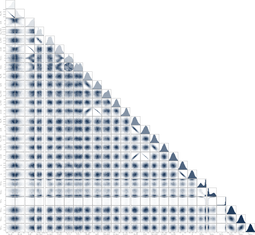
Figure 7: Joint parameter distributions when planet f is constrained to be an oblate ellipsoid with non-negative flattening.

Table 2: Means and uncertainties on fit parameters.

Parameter	Symbol	Fit value
Planet b
Radius ratio	$R_{p,\text{b}}/R_{\star}$	$0.018721\begin{subarray}{c}+0.00027939\\ -0.00025983\end{subarray}$
Orbital period (days)	$P_{\text{orb},\text{b}}$	$15.571\begin{subarray}{c}+0.00098596\\ -0.0012883\end{subarray}$
Orbital distance during transit	$d_{\text{b}}/R_{\star}$	$21.814\begin{subarray}{c}+1.1758\\ -1.13673\end{subarray}$
Complement of inclination angle (rad)	$\beta_{\text{b}}$	$0.018502\begin{subarray}{c}+0.0072221\\ -0.0056874\end{subarray}$
Planet d
Radius ratio	$R_{p,\text{d}}/R_{\star}$	$0.025600\begin{subarray}{c}+0.00040441\\ -0.00036617\end{subarray}$
Orbital period (days)	$P_{\text{orb},\text{d}}$	$278.36\begin{subarray}{c}+0.00048428\\ -0.00045518\end{subarray}$
Orbital distance during transit	$d_{\text{d}}/R_{\star}$	$148.52\begin{subarray}{c}+9.9474\\ -10.985\end{subarray}$
Complement of inclination angle (rad)	$\beta_{\text{d}}$	$0.0035144\begin{subarray}{c}+0.00094993\\ -0.00091975\end{subarray}$
Planet f
Polar radius ratio	$R_{a,\text{f}}/R_{\star}$	$0.064585\begin{subarray}{c}+0.0013792\\ -0.0023674\end{subarray}$
Equatorial radius ratio	$R_{bc,\text{f}}/R_{\star}$	$0.068592\begin{subarray}{c}+0.0026876\\ -0.0014728\end{subarray}$
Orbital period (days)	$P_{\text{orb},\text{f}}$	$542.08\begin{subarray}{c}+0.00019525\\ -0.00019565\end{subarray}$
Orbital distance during transit	$d_{\text{f}}/R_{\star}$	$230.12\begin{subarray}{c}+2.5067\\ -3.5192\end{subarray}$
Obliquity parameters	$\Gamma_{\text{f}}\cos\gamma_{\text{f}}$	$0.0056574\begin{subarray}{c}+0.54109\\ -0.55935\end{subarray}$
	$\Gamma_{\text{f}}\sin\gamma_{\text{f}}$	$0.0055163\begin{subarray}{c}+0.58152\\ -0.57378\end{subarray}$
Complement of inclination angle (rad)	$\beta_{\text{f}}$	$0.00075624\begin{subarray}{c}+0.00032842\\ -0.00035115\end{subarray}$
Common parameters
Limb darkening coefficients	$q_{1}$	$0.27330\begin{subarray}{c}+0.021219\\ -0.019876\end{subarray}$
	$q_{2}$	$0.38856\begin{subarray}{c}+0.033236\\ -0.032573\end{subarray}$
Matérn-3/2 timescale	$\log\rho_{M,\text{lc}}$	$-3.7164\begin{subarray}{c}+0.75334\\ -0.61194\end{subarray}$
	$\log\rho_{M,\text{sc}}$	$-5.4888\begin{subarray}{c}+0.088691\\ -0.094804\end{subarray}$
Matérn-3/2 amplitude	$\log\sigma_{M,\text{lc}}$	$-10.382\begin{subarray}{c}+0.34182\\ -0.25905\end{subarray}$
	$\log\sigma_{M,\text{sc}}$	$-9.9487\begin{subarray}{c}+0.028058\\ -0.027524\end{subarray}$
Jitter amplitude	$\log\sigma_{J,\text{lc}}$	$-10.348\begin{subarray}{c}+0.14883\\ -2.2985\end{subarray}$
	$\log\sigma_{J,\text{sc}}$	$-9.2709\begin{subarray}{c}+0.0070488\\ -0.0069089\end{subarray}$

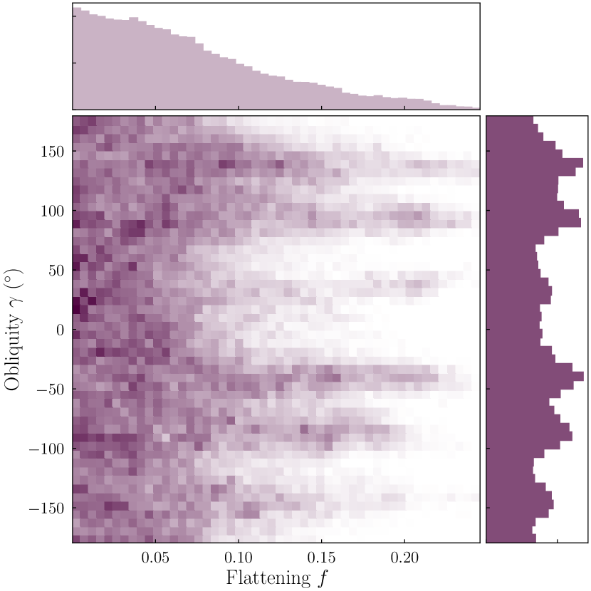
Figure 8: Joint distribution of flattening $f$ and obliquity $\gamma$ for HIP 41378 f, derived from the transit light curve fitting using the model described in Section 2. The central panel displays the density of solutions in the $f$–$\gamma$ parameter space, with darker shades indicating a higher density of allowed solutions. The marginal histograms above and to the right of the central panel show the projected distributions of $f$ and $\gamma$, respectively. These distributions highlight the range of possible planetary shapes (flattening $f$; lower values are more strongly preferred) and axial tilts (obliquity $\gamma$; all values are technically allowed by the model). The results suggest a wide range of possible obliquities, indicating a range of potential dynamical histories and orientations of HIP 41378 f.

In Figure 8, we present the joint distribution of flattening $f$ and obliquity $\gamma$ for HIP 41378 f. This constraint on planetary flattening provides an opportunity to constrain the planetary rotation period of HIP 41378 f. The rotation period of an exoplanet $P_{\text{rot}}$ and its flattening $f$ are related by

$$P_{\text{rot}}=2\pi\sqrt{\frac{R_{\text{eq}}^{3}}{GM_{p}\left(2f-3J_{2}\right)}},$$ (23)

where $G$ is the Newtonian gravitational constant, $R_{\text{eq}}$ is the equatorial radius, $M_{p}$ is the mass, and $J_{2}$ is the second spherical mass moment (Hubbard, 1984; Carter & Winn, 2010). $J_{2}$ and $f$ are not independent, since a flattened planet can have a different interior structure than its spherical counterpart. For a body with no mass asymmetry, $J_{2}=0$, while more oblate bodies have larger $J_{2}$ values: for example, Jupiter has a $J_{2}=0.15$. $J_{2}$ depends on the unknown interior structure of HIP 41378 f, so a direct measurement of $P_{\text{rot}}$ is not possible even with the constraints we have derived on HIP 41378 f’s flattening $f$. However, as inspection of Equation 23 will reveal, the effect of a larger $J_{2}$ moment is to increase the inferred planetary rotational period. As such, the rotational period calculated using Equation 23 under the assumption $J_{2}=0$ (as done in Seager & Hui, 2002) will provide a lower limit on the planetary rotational period. Using our derived posterior on $f$, we compute a distribution of computed rotation periods for HIP 41378 f, under the assumption $J_{2}=0$. We place a lower limit $P_{\text{rot}}\geq 22.2$ hr on the rotation period of HIP 41378 f, as well as an upper limit of $f\leq 0.18$ on the planet’s flattening, both at the 95% confidence level.

In Figure 9, we show one randomly-drawn model from the posterior distribution and the result of increasing the flattening of that model to $f=0.25$. The more spherical model is favored over the flattened one.

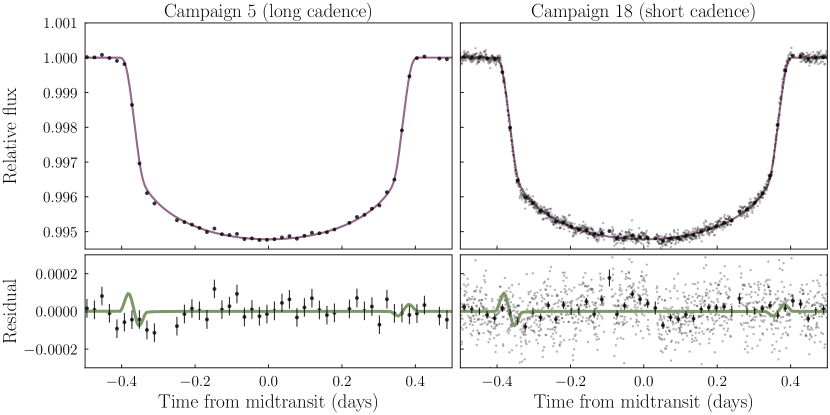
Figure 9: Long- and short-cadence transit light curve data for HIP 41378 f, folded with orbital period $P_{\text{orb}}=542.08$ days. The reduced long-cadence data is shown in the left panels in scattered points; the short-cadence data is shown on the right with small points, then binned to 30 minutes and plotted with large points. The purple curve shows a randomly-drawn model from the posterior for comparison. The lower row presents the residual between the model and the data. If the model is artificially given flattening $f=0.25$, we obtain the green curve, shown in the lower panels as a residual.

5 Discussion

In this paper, we introduce greenlantern: a new GPU-accelerated code designed to fit transit light curves of ellipsoidal planets. This code demonstrates high accuracy when compared to existing models that assume spherical planets, and it maintains competitive time performance, especially for use cases requiring large numbers of samples.

We then apply this code to the cold super-puff HIP 41378 f and establish a lower limit to its rotation period of $P_{\text{rot}}\geq 22.2$ hours. Rotation rates have previously been measured or constrained for a small number of directly imaged planets through spectroscopy (Wang et al., 2021; Parker et al., 2024; Morris et al., 2024) and a small number of massive short-period planets via transit data (Carter & Winn, 2010; Zhu et al., 2014; Biersteker & Schlichting, 2017). The ability to constrain planetary rotation and obliquity with this new code, particularly for lower-mass planets, will allow a new dimension of constraints on the processes of planet formation.

5.1 Implications for formation

This work reveals a broad range of possible obliquities for HIP 41378 f (Figure 8). While giant planets can attain primordial planetary obliquities via interactions with the circumplanetary disk (Martin & Armitage, 2021) or disk fragmentation (Jennings & Chiang, 2021), HIP 41378 f’s low mass ($12\pm 3M_{\oplus}$; Santerne et al., 2019) precludes both of these mechanisms. For planets of this mass, large obliquities could plausibly arise from dynamical interactions between planets including spin-orbit resonances (Ward & Hamilton, 2004; Li, 2021; Millholland & Laughlin, 2019; Saillenfest et al., 2019; Millholland et al., 2024), interactions between planets and their satellites (Saillenfest & Lari, 2021; Saillenfest et al., 2022), interactions between the protoplanetary disk and a young planet (Millholland & Batygin, 2019; Su & Lai, 2020), or collisions between the planet and another object in the system (Slattery et al., 1992; Morbidelli et al., 2012). Confirming a significant obliquity for HIP 41378 f would be significant, especially since this planet has no known nearby companion planets to drive strong planet-planet interactions (its nearest known companion planet, HIP 41378 e, has an approxmiate period ratio of $P_{\mathrm{orb,f}}/P_{\mathrm{orb,e}}\approx 1.46$, Santerne et al., 2019). For long-period planets like HIP 41378 f, large obliquities or rapid rotation rates offer important clues about past planet-planet interactions and the historical spacing within planetary systems, as discussed by Li & Lai (2020). The processes driving the rotational evolution of cold planets are markedly different from those affecting hot Jupiters, which often undergo dynamical erasure of their histories via tidal interactions and therefore offer less insight towards their formation histories.

Based on the derived rotation period limit for HIP 4138 f derived in this work, it is likely that HIP 41378 f is a less rapid rotator than the Solar System gas giants. While the quality of the current light curve is insufficient to securely measure HIP 41378 f’s obliquity, improved constraints with future data would allow a more direct test of the importance of past impacts or planet-disk interactions in setting its current dynamical state.

5.2 Possibility of rings

HIP 41378 f has a Jupiter-like radius ($9.2\pm 0.1R_{\oplus}$; Vanderburg et al., 2016a), sub-Neptune mass ($12\pm 3M_{\oplus}$; Santerne et al., 2019), and an anomalously low density (0.09 g cm^-3). Combined with HIP 41378 f’s low effective temperature ($\sim 294$ K; Santerne et al., 2019) and the old age of its host star ($\sim 2$ Gyr; Lund et al., 2019), the planet’s structure subverts expectations. Its range of allowable core masses are less massive than expected for a planet of this size (Belkovski et al., 2022), resulting in a theoretical challenge of how the planet attained its observed mass and density.

One explanation for its large radius could be the presence of circumplanetary rings (Akinsanmi et al., 2020; Piro & Vissapragada, 2020), possibly due to migrating and disintegrating exomoons (Saillenfest et al., 2023), which would increase the apparent planetary radius. If viewed in a face-on geometry, these rings could mimic the shape of a ringless planet. HST transmission spectra of this planet are consistent with the rings hypothesis (Alam et al., 2022), which would be expected to cause a flat transmission spectrum (Ohno & Fortney, 2022).

The results of this paper demonstrate flattening of $f\leq 0.18$ is consistent with the shape of the transit light curve. In Section 4, we discuss how this constrained amount of flattening can be used to infer the planetary rotation rate, assuming that rotational deformation is the primary cause of non-sphericity. However, it is important to note that if HIP 41378 f does host circumplanetary rings, the observed flattening would not be due to the planet’s rotation, but rather the geometry of the rings. Consequently, in that case, our stated constraints on the planet’s rotation would no longer apply.

5.3 Improving constraint with JWST

As demonstrated in Figure 5, the signal that allows the detection of flattening in a light curve is small in amplitude and occurs at transit ingress and egress only. As a result, such measurements can only be made with sufficiently high-precision and high-cadence data. In this work, we use K2 data on a long-period planet; however, this data quality provides only an upper limit on flattening. To improve upon the constraint of this work, we need a high precision light curve to precisely characterize the exact shape of ingress and egress events. Liu et al. (2024b) demonstrates that for a Saturn-like oblateness, a greater-than-Earth-like obliquity ($>20^{\circ}$), and a Jupiter-like planet, one transit of JWST data could recover the flattening.

Table 3: Estimated noise of follow-up JWST observations.

Instrument mode	Cadence	Noise estimate (ppm)
NIRISS, substrip 256	1 min	21.71
NIRISS, substrip 256	2 min	15.35
NIRISS, substrip 96	1 min	21.71
NIRISS, substrip 96	2 min	15.35

To evaluate the improvements on the flattening constraint that would be possible for HIP 41378 f with JWST data, we simulated the expected noise for observing the transit of HIP 41378 f using PandExo (Batalha et al., 2017) for NIRISS. We focus our noise estimates on NIRISS since it has already been shown to produce high precision light curves and achieved 5 ppm RMS for 1-hour bins when observing WASP-18 b (Coulombe et al., 2023). In our PandExo simulation, we used a PHOENIX stellar model grid for the stellar properties of HIP 41378 ($T=6226$ K, $\left[\text{Fe}/\text{H}\right]=-0.11$, $\log{g}=7.982$). We generated our own custom planet model using batman and the planet parameter estimates from Berardo et al. (2019). We input this photometric light curve into PandExo. We set the saturation limit to 80% and computed noise estimates for 2 and 1 minute cadence for one transit since only one will occur during cycle 4. We find that the 2 minute cadence observations would be expected to produce 15.35 ppm of noise and the 1 minute cadence observations would produce 21.71 ppm of noise.

Based on these noise estimates, we simulate a transit light curve for HIP 41378 f with 20 ppm white noise and no red noise using a 2 minute cadence. We adopt the fit parameter values from Table 2 but inject test values for flattening ($f=0.1$), complement of inclination ($\beta=0^{\circ}$), and obliqutiy ($\gamma=15^{\circ}$), keeping the transit depth constant. We find that, if these were the true values, photometric data from JWST could definitively exclude a spherical planet shape, $f=0$. The joint posterior of flattening and obliquity is shown in Figure 10.

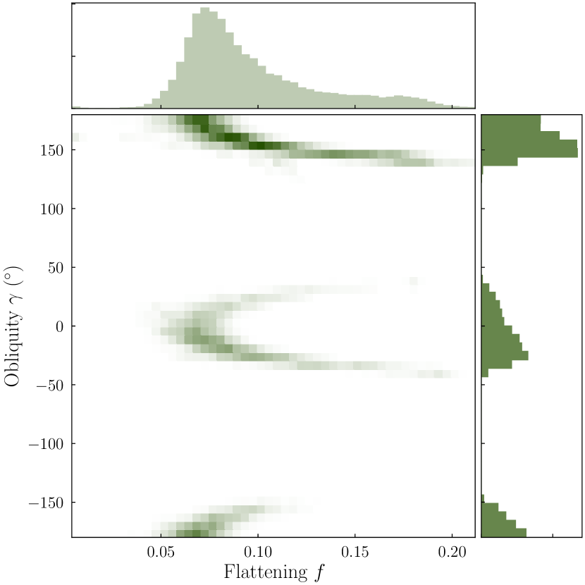
Figure 10: Joint posterior of flattening and obliquity for a simulated light curve of a flattened planet with $f=0.1$. For this test case, fitting with greenlantern excludes the $f=0$ model.

6 Conclusions

In this paper, we present a constraint on the rotation period of a sub-Neptune-mass exoplanet, HIP 41378 f, using K2 transit light curve data. By developing and applying a new GPU-accelerated code, greenlantern, which models the transits of ellipsoidal planets, we are able to derive posterior distributions for the planet’s flattening and obliquity. These constraints allow us to place a lower limit on HIP 41378 f’s rotation period of $P_{\text{rot}}\geq 22.2$ hours at the 95% confidence level, suggesting a slower rotation rate than is seen for the Solar System gas giants. Future observations, especially with high-precision instruments like JWST, will allow for even tighter constraints on planetary deformation and rotation rate, further enhancing our understanding of exoplanetary formation and evolution processes.

Note in Manuscript: During the late stages of manuscript preparation, we became aware of two other works on similar topics. Cassese et al. (2024) described the development of another GPU-based code for modeling oblate planets, while Lammers & Winn (2024) reported on similar constraints on the rotation period of a different super-puff planet, Kepler 51 d. These works are complementary to ours and highlight the growing importance of oblateness measurements in the era of precise photometry from JWST.

References

- Akinsanmi et al. (2020) Akinsanmi, B., Barros, S. C. C., Santos, N. C., Oshagh, M., & Serrano, L. M. 2020, MNRAS, 497, 3484, doi: 10.1093/mnras/staa2164
- Alam et al. (2022) Alam, M. K., Kirk, J., Dressing, C. D., et al. 2022, ApJ, 927, L5, doi: 10.3847/2041-8213/ac559d
- Barnes & Fortney (2003) Barnes, J. W., & Fortney, J. J. 2003, ApJ, 588, 545, doi: 10.1086/373893
- Batalha et al. (2017) Batalha, N. E., Mandell, A., Pontoppidan, K., et al. 2017, PASP, 129, 064501, doi: 10.1088/1538-3873/aa65b0
- Becker et al. (2019) Becker, J. C., Vanderburg, A., Rodriguez, J. E., et al. 2019, AJ, 157, 19, doi: 10.3847/1538-3881/aaf0a2
- Belkovski et al. (2022) Belkovski, M., Becker, J., Howe, A., Malsky, I., & Batygin, K. 2022, AJ, 163, 277, doi: 10.3847/1538-3881/ac6353
- Berardo & de Wit (2022) Berardo, D., & de Wit, J. 2022, ApJ, 935, 178, doi: 10.3847/1538-4357/ac82b2
- Berardo et al. (2019) Berardo, D., Crossfield, I. J. M., Werner, M., et al. 2019, AJ, 157, 185, doi: 10.3847/1538-3881/ab100c
- Biersteker & Schlichting (2017) Biersteker, J., & Schlichting, H. 2017, AJ, 154, 164, doi: 10.3847/1538-3881/aa88c2
- Bryan et al. (2021) Bryan, M. L., Chiang, E., Morley, C. V., Mace, G. N., & Bowler, B. P. 2021, AJ, 162, 217, doi: 10.3847/1538-3881/ac1bb1
- Bryan et al. (2020) Bryan, M. L., Chiang, E., Bowler, B. P., et al. 2020, AJ, 159, 181, doi: 10.3847/1538-3881/ab76c6
- Carado & Knuth (2020) Carado, B., & Knuth, K. H. 2020, Astronomy and Computing, 32, 100406, doi: 10.1016/j.ascom.2020.100406
- Carter & Winn (2010) Carter, J. A., & Winn, J. N. 2010, ApJ, 709, 1219, doi: 10.1088/0004-637X/709/2/1219
- Cassese et al. (2024) Cassese, B., Vega, J., Lu, T., et al. 2024, arXiv e-prints, arXiv:2409.00167, doi: 10.48550/arXiv.2409.00167
- Coulombe et al. (2023) Coulombe, L.-P., Benneke, B., Challener, R., et al. 2023, Nature, 620, 292, doi: 10.1038/s41586-023-06230-1
- Eastman (2024) Eastman, J. D. 2024, PASP, 136, 014502, doi: 10.1088/1538-3873/ad1412
- Foreman-Mackey et al. (2017) Foreman-Mackey, D., Agol, E., Ambikasaran, S., & Angus, R. 2017, AJ, 154, 220, doi: 10.3847/1538-3881/aa9332
- Foreman-Mackey et al. (2013) Foreman-Mackey, D., Hogg, D. W., Lang, D., & Goodman, J. 2013, PASP, 125, 306, doi: 10.1086/670067
- Harada et al. (2023) Harada, C. K., Dressing, C. D., Alam, M. K., et al. 2023, AJ, 166, 208, doi: 10.3847/1538-3881/ad011c
- Hubbard (1984) Hubbard, W. B. 1984, Planetary interiors
- Jennings & Chiang (2021) Jennings, R. M., & Chiang, E. 2021, MNRAS, 507, 5187, doi: 10.1093/mnras/stab2429
- Kipping (2013) Kipping, D. M. 2013, MNRAS, 435, 2152, doi: 10.1093/mnras/stt1435
- Kreidberg (2015) Kreidberg, L. 2015, PASP, 127, 1161, doi: 10.1086/683602
- Lammers & Winn (2024) Lammers, C., & Winn, J. N. 2024, Slow Rotation for the Super-Puff Planet Kepler-51d. https://arxiv.org/abs/2409.06697
- Laskar & Robutel (1993) Laskar, J., & Robutel, P. 1993, Nature, 361, 608, doi: 10.1038/361608a0
- Leconte et al. (2011) Leconte, J., Lai, D., & Chabrier, G. 2011, A&A, 528, A41, doi: 10.1051/0004-6361/201015811
- Li (2021) Li, G. 2021, ApJ, 915, L2, doi: 10.3847/2041-8213/ac0620
- Li & Lai (2020) Li, J., & Lai, D. 2020, ApJ, 898, L20, doi: 10.3847/2041-8213/aba2c4
- Liu et al. (2024a) Liu, Q., Zhu, W., Zhou, Y., et al. 2024a, arXiv e-prints, arXiv:2406.11644, doi: 10.48550/arXiv.2406.11644
- Liu et al. (2024b) —. 2024b, arXiv e-prints, arXiv:2406.11644, doi: 10.48550/arXiv.2406.11644
- Lund et al. (2019) Lund, M. N., Knudstrup, E., Silva Aguirre, V., et al. 2019, AJ, 158, 248, doi: 10.3847/1538-3881/ab5280
- Martin & Armitage (2021) Martin, R. G., & Armitage, P. J. 2021, ApJ, 912, L16, doi: 10.3847/2041-8213/abf736
- Millholland & Batygin (2019) Millholland, S., & Batygin, K. 2019, ApJ, 876, 119, doi: 10.3847/1538-4357/ab19be
- Millholland & Laughlin (2019) Millholland, S., & Laughlin, G. 2019, Nature Astronomy, 3, 424, doi: 10.1038/s41550-019-0701-7
- Millholland et al. (2024) Millholland, S. C., Lara, T., & Toomlaid, J. 2024, ApJ, 961, 203, doi: 10.3847/1538-4357/ad10a0
- Morbidelli et al. (2012) Morbidelli, A., Tsiganis, K., Batygin, K., Crida, A., & Gomes, R. 2012, Icarus, 219, 737, doi: 10.1016/j.icarus.2012.03.025
- Morris et al. (2024) Morris, E. C., Wang, J. J., Hsu, C.-C., et al. 2024, arXiv e-prints, arXiv:2405.13125, doi: 10.48550/arXiv.2405.13125
- Ohno & Fortney (2022) Ohno, K., & Fortney, J. J. 2022, arXiv e-prints, arXiv:2201.02794. https://arxiv.org/abs/2201.02794
- Pál (2012) Pál, A. 2012, MNRAS, 420, 1630, doi: 10.1111/j.1365-2966.2011.20151.x
- Parker et al. (2024) Parker, L. T., Birkby, J. L., Landman, R., et al. 2024, MNRAS, 531, 2356, doi: 10.1093/mnras/stae1277
- Piro & Vissapragada (2020) Piro, A. L., & Vissapragada, S. 2020, AJ, 159, 131, doi: 10.3847/1538-3881/ab7192
- Saillenfest & Lari (2021) Saillenfest, M., & Lari, G. 2021, A&A, 654, A83, doi: 10.1051/0004-6361/202141467
- Saillenfest et al. (2019) Saillenfest, M., Laskar, J., & Boué, G. 2019, A&A, 623, A4, doi: 10.1051/0004-6361/201834344
- Saillenfest et al. (2022) Saillenfest, M., Rogoszinski, Z., Lari, G., et al. 2022, A&A, 668, A108, doi: 10.1051/0004-6361/202243953
- Saillenfest et al. (2023) Saillenfest, M., Sulis, S., Charpentier, P., & Santerne, A. 2023, A&A, 675, A174, doi: 10.1051/0004-6361/202346745
- Santerne et al. (2019) Santerne, A., Malavolta, L., Kosiarek, M. R., et al. 2019, arXiv e-prints, arXiv:1911.07355, doi: 10.48550/arXiv.1911.07355
- Seager & Hui (2002) Seager, S., & Hui, L. 2002, ApJ, 574, 1004, doi: 10.1086/340994
- Slattery et al. (1992) Slattery, W. L., Benz, W., & Cameron, A. G. W. 1992, Icarus, 99, 167, doi: 10.1016/0019-1035(92)90180-F
- Storn & Price (1997) Storn, R., & Price, K. 1997, Journal of Global Optimization, 11, 341, doi: 10.1023/A:1008202821328
- Su & Lai (2020) Su, Y., & Lai, D. 2020, ApJ, 903, 7, doi: 10.3847/1538-4357/abb6f3
- Vanderburg & Johnson (2014) Vanderburg, A., & Johnson, J. A. 2014, PASP, 126, 948, doi: 10.1086/678764
- Vanderburg et al. (2016a) Vanderburg, A., Becker, J. C., Kristiansen, M. H., et al. 2016a, ApJ, 827, L10, doi: 10.3847/2041-8205/827/1/L10
- Vanderburg et al. (2016b) Vanderburg, A., Latham, D. W., Buchhave, L. A., et al. 2016b, ApJS, 222, 14, doi: 10.3847/0067-0049/222/1/14
- Virtanen et al. (2020) Virtanen, P., Gommers, R., Oliphant, T. E., et al. 2020, Nature Methods, 17, 261, doi: 10.1038/s41592-019-0686-2
- Wang et al. (2021) Wang, J. J., Ruffio, J.-B., Morris, E., et al. 2021, AJ, 162, 148, doi: 10.3847/1538-3881/ac1349
- Ward & Hamilton (2004) Ward, W. R., & Hamilton, D. P. 2004, AJ, 128, 2501, doi: 10.1086/424533
- Zhu et al. (2014) Zhu, W., Huang, C. X., Zhou, G., & Lin, D. N. C. 2014, ApJ, 796, 67, doi: 10.1088/0004-637X/796/1/67