GreenLight-Gym: A Reinforcement Learning Benchmark Environment for Greenhouse Crop Production Control

Abstract

Controlling greenhouse crop production is complex due to uncertain and non-linear dynamics between crops, indoor and outdoor climate, and economics. Due to declining skilled growers, autonomous greenhouse control systems are required. Reinforcement learning (RL) is a machine learning framework that can learn a control policy to automate the control of a greenhouse. This control policy is optimised through numerous interactions with (a model of) the greenhouse, guided by an economic-based reward function. Despite RL’s potential, its application to real-world greenhouse systems is limited. This is mainly because policies are learned over models with discrepancies in the dynamics regarding real-world greenhouse systems. Additionally, RL algorithms can struggle to maintain imposed state constraints while optimising for the primary objective. In particular, if the greenhouse model does not accurately capture these constraints’ adverse effects on crop growth. Finally, generalisation to unseen states, for instance, due to novel weather trajectories, is rarely examined for RL-based control in greenhouse crop production. This work makes three key contributions to address these challenges and advance the application of RL in greenhouse crop production control. First, we introduce GreenLight-Gym, to the best of our knowledge, the first open-source environment designed for training and testing RL algorithms on the state-of-the-art greenhouse model GreenLight. GreenLight-Gym facilitates monitoring the progress of RL-based control methodologies by the greenhouse control community. Second, simulation experiments examine two approaches adhering to state boundaries by penalising the reward function either with a multiplicative or an additive reward. These experiments show that the additive penalty has a more stable training process converging to similar control policies when randomly initialised. Also, the additive reward approach satisfies state constraints more frequently. In contrast, the multiplicative reward achieves slightly higher profits. Finally, RL controller performance is compared between a disjoint training and testing weather dataset to demonstrate the generalisation capability across unseen weather conditions. This experiment demonstrates that extensively training RL controllers on various weather trajectories enhances their ability to generalise to weather trajectories, which are assumed to have a similar underlying distribution. The environment and the scripts for experiments and training the RL controller are available as open-source software at https://github.com/BartvLaatum/GreenLightGym. This study and its accompanying open-source software aim to stimulate the development of innovative learning-based control algorithms for greenhouse crop production within the greenhouse control community. It also allows for comparing the developed algorithms to standard state-of-the-art practice controllers.

GreenLight-Gym: Open-source simulator for greenhouse climate-crop dynamics and control.

First simulator designed to train reinforcement learning controllers for crop production.

Two RL controllers with different reward functions evaluated using GreenLight-Gym.

Both reward functions showed stable behaviour during learning and evaluation.

Controllers demonstrated generalising capabilities to novel weather trajectories.

1 Introduction

Recent studies expect an increase of the global food demand between 35%-56% between 2010 and 2050 as a result of anthropogenic factors, like population growth, urbanisation and demographic dynamics (Abbasi et al., 2022; FAO, 2022; Van Dijk et al., 2021). The encroachment of rural areas due to urbanisation raises the demand to efficiently produce fresh food near urban areas without polluting the environment (Marcelis and Heuvelink, 2019).

Greenhouse horticulture can produce large amounts of food by providing a shelter for crops to protect them against unpredictable outdoor weather events and offering more facets to control their environment (Stanghellini et al., 2019; Van Henten et al., 2012). Despite their potential position in the future food supply chain, greenhouse systems face severe challenges like their large carbon footprint. From 2015 to 2021, the industry’s total carbon dioxide emission has been growing again (Smit, 2023). The sector accounts for nearly 7% of the natural gas consumption in the Netherlands (De Ruyter et al., 2021). To maintain high yields per unit area while under the scrutiny of sustainability goals, greenhouse growers must maintain an ideal growing climate for their crops while minimising resource consumption. However, the sector struggles to find skilled growers for efficient greenhouse crop production even though facilities keep expanding, necessitating more labour to monitor all the details of greenhouse compartments (Sparks, 2018; Van der Meulen, 2022).

Managing greenhouse crop production involves uncertain, complex, and non-linear interactions among crop growth dynamics, indoor and outdoor climate conditions, energy systems, and economic factors, and where decisions can affect performance weeks later (Holder and Cockshull, 1990). Optimising an economic objective by maximising crop production while minimising resource consumption is a primary direction of research (Iddio et al., 2020). Good economic performance requires a controller that can manipulate the indoor climate variables through fine-grained control of several greenhouse actuators to maintain an ideal growing climate for the crop, i.e., the greenhouse production control problem.

Previous studies along these lines explored advanced control techniques, like model-predictive control (MPC), which tackles the greenhouse control problem by designing a dynamical model of the greenhouse system and solving a finite horizon control problem by optimising its objective after each time step in an online manner (Boersma et al., 2022; Kuijpers et al., 2021; Van Henten, 1994; Xu et al., 2018). This domain of controllers performs effectively, especially when minimising resource consumption within predefined climate boundaries (Van Beveren et al., 2020). However, these methods can struggle to handle realistic uncertainties from unmodelled dynamics, weather forecasts or sensor noise, affecting their performance (Morcego et al., 2023). Kuijpers et al. (2022) aimed to deal with uncertainties in weather forecasts by applying randomised MPC. However, their approach could only sample three weather scenarios due to computational limitations, not fully covering the uncertainty space from their weather forecast model. Moreover, these methods encounter challenges with increased model complexity, making them rely on simplified models, which raised concerns about model quality (precision) and consequently limited their adoption in practice (Morcego et al., 2023; Picard et al., 2017; Van Straten, 1999).

Reinforcement Learning (RL) is a promising framework for addressing the greenhouse control problem. RL approximates optimal control policies, i.e., controller, from non-linear and high-dimensional inputs to maximise a feedback signal, i.e., reward. In contrast with previous control approaches, RL computes the control policy before deployment, enabling it to characterise uncertainty and how it affects the control performance during the learning process. This makes the controller more robust against those uncertainties when generalising control policies learned during simulation to real-world systems (Song et al., 2023). RL has already been successful in domains like gaming, where it directly learned from the actual system (Mnih et al., 2015; Silver et al., 2018; Vinyals et al., 2019), in robotics, where system dynamics are well-known (Kaufmann et al., 2023; OpenAI et al., 2019), and also in physically challenging environments, like navigating stratospheric balloons (Bellemare et al., 2020), and controlling tokamak plasma through precise control of the magnetic coils (Degrave et al., 2022). RL thrived in these fields by exploring the system dynamics through a vast amount of interactions with a model of the system. Despite its success in these domains, greenhouse crop production raises new challenges for RL before the application in a real-world greenhouse is possible. Because RL algorithms require millions of interactions to learn a reasonable control policy, it is infeasible to let RL algorithms directly learn from interactions with a physical greenhouse. This is mainly because crop growth cycles are lengthy, e.g., the tomato production season runs close to a year (Vermeulen, 2008).

Existing literature deals with this challenge by using models to approximate control policies in silico. Tchamitchian et al. (2005) and Morcego et al. (2023) applied RL algorithms to learn control policies from interactions with a process-based greenhouse model. Since these models rely on simplified dynamics that do not capture the true complexity of the greenhouse crop production systems, their learned control policies likely fail to generalise to real-world greenhouse systems. This issue correlates to the challenge faced by the advanced control techniques mentioned earlier. Model-based reinforcement learning (MBRL) addresses this problem by identifying a greenhouse model from real-world data using black-box function approximators (An et al., 2021; Cao et al., 2022). Zhang et al. (2021) extended this MBRL framework with probabilistic ensemble models to handle uncertainty regarding indoor climate disturbances to obtain robust control policies. However, MBRL relies on the quality of the data to approximate a greenhouse model, and their black-box models struggle to generalise to new situations. For example, when novel weather trajectories are encountered, crop species are altered or greenhouse facilities change. Moreover, none of these studies reported their results on benchmark environments, as each study approximated control policies on different greenhouse crop production models. This complicates monitoring and comparing the progress of RL-based approaches in greenhouse control.

To address these limitations and provide a standardised platform for RL research in greenhouse control, a new benchmark environment is needed. Therefore, this work introduces GreenLight-Gym, an RL environment to train, test and compare control policies for greenhouse crop production systems. This environment replicates greenhouse dynamics and provides a standardised benchmark for designing and enhancing RL algorithms in greenhouse control. GreenLight-Gym encapsulates a greenhouse simulator based on the state-of-the-art dynamical GreenLight model (Katzin et al., 2020). GreenLight is a detailed and validated greenhouse model that accurately captures the climate-crop dynamics of high-tech greenhouse facilities, incorporating more complex interactions and variables than the simplified greenhouse models used in previous advanced control and RL methods. Besides, its process-based nature facilitates the natural extension to a wide range of greenhouse facilities by adjusting model parameters.

GreenLight-Gym reimplemented GreenLight in high-performance code to facilitate rapid controller-environment interactions required to train RL algorithms. To validate this reimplementation as a reliable model of the greenhouse system, the state dynamics are verified against GreenLight’s original Matlab code. Also, an analysis of the execution time of both implementations is included. The modular nature of this environment invites researchers to study RL-based control methods (or other types of control methods) in user-defined greenhouse systems by specifying controllers, rewards and constraints, observation spaces, model parameters, weather disturbances, and controllable inputs. By using GreenLight-Gym as a benchmark environment for RL-based greenhouse control, the progress of this new methodologies becomes trackable. Subsection 2.5 provides a detailed description of the software’s modular components.

The modular design of GreenLight-Gym addresses another critical issue widely discussed in RL literature: generalisation to unseen environments. Zhang et al. (2018) showed that deep RL algorithms are prone to overfitting on a single configuration of the training environment, resulting in memorisation of the training data rather than learning generalisable control policies. This can lead to poor performance when evaluated in unseen environments. However, increasing the diversity in the training data can significantly improve the generalisation capabilities of those RL algorithms (Kirk et al., 2023; Zhang et al., 2018). In the context of greenhouse horticulture, training data diversity can be achieved by variations in the weather trajectories and greenhouse model dynamics. To the best of our knowledge, none of the existing works on RL for greenhouse crop production control have used disjoint train and test environments to evaluate their methods. Potentially, they disregard the generalisation aspect of their approaches. GreenLight-Gym’s modular architecture addresses this gap by allowing users to easily randomise the training environment, for instance, by sampling weather trajectories over a broad period of historical dates. Furthermore, the open-source software facilitates the generation of disjoint test environments, enabling the assessment of generalisation capabilities of RL methods on greenhouse crop production systems.

Besides generalisation and overfitting, another challenge in training an RL controller is mitigating unfavourable states. Current crop simulation models can only accurately predict crop yield within defined climatic boundaries (Vanthoor et al., 2011a). However, beyond these established boundaries, the impacts on crop growth and quality still need to be discovered. Therefore, advanced control algorithms, like MPC, impose boundaries on state variables because the models are based on assumptions and can produce unrealistic predictions outside these known boundaries (Boersma et al., 2022; Tap, 2000; Van Henten, 1994). Dealing with constraints, e.g., on state boundaries, is a known challenge for RL algorithms (Dulac-Arnold et al., 2021; Liu et al., 2021). Seminal works focused on Lagrange relaxation by adding a penalty term to the reward function, controlled through adaptive Lagrange multipliers (Bohez et al., 2019; Chow et al., 2017; Tessler et al., 2018). However, this approach is sensitive to the initialisation of the Lagrange multipliers and the learning rate. Constrained policy optimisation and Interior-point policy optimisation (IPO) extend existing policy optimisation algorithms (Schulman et al., 2015, 2017) to incorporate constraints but can be computationally inefficient and complex or require a feasible policy upon initialisation (Achiam et al., 2017; Liu et al., 2020). In RL, reward shaping is a widely used technique where manually designed feedback signals penalise the controller’s behaviour to avoid undesired states (Bellemare et al., 2020; Degrave et al., 2022; Peng et al., 2018; Wurman et al., 2022). While reward shaping can handle multiple constraints simultaneously and is convenient to implement, its success hinges on precise tuning to balance the trade-off between reward maximisation and constraint violations, often conflicting terms.

This work leverages the GreenLight-Gym framework to train and evaluate a reinforcement learning controller for greenhouse crop production systems. This controller aims to optimise a profit-based objective function that balances fruit harvest revenue against resource costs while maintaining state variables within predefined boundaries. To enforce these state constraints, this study employs reward-shaping techniques to penalise undesired behaviour. Specifically, two methods for penalising boundary violations are evaluated: (1) the additive penalty approach, which subtracts a penalty value from the reward, and (2) the multiplicative penalty approach, which modulates the reward via multiplication. A sensitivity analysis is conducted to provide insight into how penalty coefficients of both approaches impact the control performance. Contrasting previous work, this study defines a simulation benchmark as a disjoint weather dataset for evaluating controller performance. This test set assesses the controller’s ability to generalise to novel weather trajectories. The training dataset spans a decade (2011-2020), between March and September, to introduce sufficient variability and enhance the controller’s capacity to generalise to the disjoint test set. For a detailed description of the simulation experiments and results, the reader is referred to Sections 3 & 4.

In summary, the main contributions of this work are fourfold:

• GreenLight-Gym is introduced, a benchmark environment for training and evaluating RL algorithms. To establish GreenLight-Gym as a reliable benchmark, its state dynamics are verified against the original Matlab implementation of GreenLight.

• A reinforcement learning-based controller learns to control the indoor greenhouse climate by optimising a profit-based objective while adhering to state boundaries using the GreenLight-Gym’s framework. The stability and performance of this controller are assessed by analysing convergence metrics during training.

• A sensitivity analysis asserts the impact on controller performance for two different approaches for penalising undesired behaviour through the reward function.

• RL controller performance is compared between a disjoint training and testing weather dataset, demonstrating the generalisation capability across unseen weather conditions.

The further outline of this paper is organised as follows: Section 2 formally introduces the concepts and works the modular GreenLight-Gym framework builds upon. Specifically, the GreenLight model, the greenhouse control problem, reinforcement learning, and the optimisation method are discussed in subsections 2.1, 2.2, 2.3 & 2.4. Next, GreenLight-Gym’s modular components are presented in subsection 2.5. Section 3 presents the simulation experiments conducted using the environment, and Section 4 presents their results. The assumptions and limitations of the environment and the simulation experiments are discussed in Section 5. Finally, Section 6 draws conclusions and recommendations for future work.

2 Components of the GreenLight-Gym software suite

Reinforcement learning algorithms are known to be data-inefficient, necessitating extensive interactions to learn control policies, i.e., controllers. This work introduces GreenLight-Gym to address this challenge within the context of greenhouse crop production systems. GreenLight-Gym is a benchmark environment designed to train, test, and monitor the progress of RL-based controllers on greenhouse control problems. This section explicates the capabilities of the GreenLight-Gym environment as a software suite. Specifically, subsection 2.1 describes the GreenLight model upon which the environment is based. Next, the greenhouse control problem, reinforcement learning for greenhouse control applications, and the policy gradient optimisation method used during this study are formally defined in subsections 2.2, 2.3, and 2.4, respectively. Finally, subsection 2.5 details the GreenLight-Gym environment, including its seven customisable modules.

2.1 GreenLight

GreenLight is a state-of-the-art, open-source, dynamic process-based model designed for greenhouse climate simulations in high-tech horticulture facilities (Katzin et al., 2020). It incorporates supplementary lighting to capture its influence on the greenhouse climate and crop by extending Vanthoor et al. (2011b) climate model and employing a crop yield model Vanthoor et al. (2011a). The system’s dynamics are represented by the following system of ordinary differential equations (ODEs)

$$\dot{x}(t)=f(x(t),u(t),d(t),p),$$ (1)

where $x\in\mathbb{R}^{n_{x}}$ represents the state of the greenhouse system consisting of indoor climate and crop variables, $u\in\mathbb{R}^{n_{u}}$ is the controllable input that affects the indoor climate, $d\in\mathbb{R}^{n_{d}}$ is the non-controllable input, i.e., weather disturbance and $p\in\mathbb{R}^{n_{p}}$ contains the model parameters. Following GreenLight, the control inputs represent valve settings of greenhouse actuators, where 0 indicates no action (lights off, an open screen) and 1 indicates the actuator is at maximum capacity (lights on, a fully closed screen). The valves for the boiler and $\mathrm{CO_{2}}$-injection have corresponding capacities that determine the absolute heating energy and $\mathrm{CO_{2}}$ input to the greenhouse. In Tables 1 & 2, the state variables and controllable inputs of the GreenLight model are described. For a detailed description of the dynamical model $f(\cdot)$, the reader is referred to (Katzin et al., 2020).

State Variable	Unit	Description
CO${}_{2,\text{air}}$	$\mathrm{mg\{CO_{2}\}/m^{3}}$	CO2 concentration the the main air compartment
CO${}_{2,\text{top}}$	$\mathrm{mg\{CO_{2}\}/m^{3}}$	CO2 concentration in the top air compartment
T${}_{\text{air}}$	°C	Air temperature in the top air compartment
T${}_{\text{top}}$	°C	Air temperature in the top air compartment
T${}_{\text{can}}$	°C	Canopy temperature
T${}_{\text{cov,in}}$	°C	Indoor cover temperature
T${}_{\text{cov,e}}$	°C	Outdoor cover temperature
T${}_{\text{thscr}}$	°C	Thermal screen temperature
T${}_{\text{flr}}$	°C	Floor temperature
T${}_{\text{pipe}}$	°C	Heating pipe temperature
T${}_{\text{soil1}}$	°C	First soil layer temperature
T${}_{\text{soil2}}$	°C	Second soil layer temperature
T${}_{\text{soil3}}$	°C	Third soil layer temperature
T${}_{\text{soil4}}$	°C	Fourth soil layer temperature
T${}_{\text{soil5}}$	°C	Fifth soil layer temperature
VP${}_{\text{air}}$	Pa	Vapour pressure in main air compartment
VP${}_{\text{top}}$	Pa	Vapour pressure in top air compartment
T${}_{\text{lamp}}$	°C	Top light temperature
T${}_{\text{int,lamp}}$	°C	Inter-light temperature
T${}_{\text{gropipe}}$	°C	Grow pipe temperature
T${}_{\text{blscr}}$	°C	Blackout screen temperature
T${}_{\text{can24}}$	°C	Average canopy temperature over the last 24 hours
C${}_{\text{buf}}$	$\mathrm{mg\{CH_{2}O\}/m^{2}}$	Carbohydrates in the crops’s carbohydrates buffer
C${}_{\text{leaf}}$	$\mathrm{mg\{CH_{2}O\}/m^{2}}$	Carbohydrates in the crop’s leaves
C${}_{\text{stem}}$	$\mathrm{mg\{CH_{2}O\}/m^{2}}$	Carbohydrates in the crop’s carbohydrates stem
C${}_{\text{fruit}}$	$\mathrm{mg\{CH_{2}O\}/m^{2}}$	Carbohydrates in the crop’s fruit
T${}_{\text{cansum}}$	°C days	Temperature sum for the canopy
Time	days	Simulation time in days

Table 1: The 27 state variables of the GreenLight model, their unit, and a short description of the variable.

Control input	Lower	Upper	Description
$u_{\mathrm{CO}_{2}}$	0	1	CO2 injection into the greenhouse
$u_{\text{vent}}$	0	1	Aperture of the roof window
$u_{\text{boil}}$	0	1	Opening of valve between the boiler and heating pipes
$u_{\text{led}}$	0	1	Electrical intensity of the LED lamps
$u_{\text{thscr}}$	0	1	Closure of the thermal screen

Table 2: Controllable inputs $(u)$ of the GreenLight model. These inputs refer to the valve settings for greenhouse actuators.

2.2 Greenhouse control problem

This section formalises greenhouse crop production control as a constrained optimisation problem. The greenhouse crop production model in (1) is discretised by numerically approximating the dynamical system through $x_{k+1}=F(x_{k},u_{k},d_{k},p)$, where $F(\cdot)$ is the discrete-time version of (1), with $\Delta t$ as control interval, and $k$ the discrete-time such that $t=\Delta t\cdot k$. To accurately represent all the (fast) physical processes by the discretised system, $F(\cdot)$ runs at a smaller sampling period $\Delta t\geq h$.

Controllable input $u_{k}$ steers the system’s dynamics ($x_{k}$) at time step $k$. Given the initial state $x_{0}$, the goal is to optimise a profit-based objective by optimising $u_{k}$ while considering the outside weather $d_{k}$. The profit-based objective is defined as

$$r_{0:N}^{\text{profit}}=\sum_{k=0}^{N}r_{k}^{\text{profit}},$$ (2)

which denotes the profit made over a horizon of $N$ time steps. Here $r_{k}^{\text{profit}}$ represents a profit-based reward that encodes the profit made at time step $k$. So this objective is optimised by finding control input $u_{k}$, while taking $d_{k}$ into account at each discrete time step. The controls are held constant during control interval $\Delta t$, resulting in a piecewise constant function.

Despite the detailed description of the greenhouse crop production system by GreenLight, this model has regions in the state space where it fails to accurately describe real-world dynamics, e.g., in extreme humidity concentrations. To avoid regions with non-representative dynamics, constraints are imposed, resulting in the following constrained optimisation problem

$$\begin{split}\max_{\tau}r_{0:N}^{\mathrm{profit}}\\ \text{subject to:}&\\ x_{k+1}&=F(x_{k},u_{k},d_{k},p),\\ y_{k}&=g(x_{k},u_{k},d_{k},p),\\ \underline{\omega}&\leq z(x_{k},u_{k})\leq\overline{\omega},\\ x_{0}&=x_{\mathrm{init}},\end{split}$$ (3)

where $\tau=(x_{0},u_{0},x_{1},\dots,u_{N-1},x_{N})$ denotes the resulting sequence (trajectories) of states and control inputs. $x_{k},u_{k},d_{k},p$ are defined similarly to (1). $y_{k}$ represents system observations and could be any measurement computed from states, control inputs, disturbances and model parameters. The inequality equations $z(\cdot)$ represent the system constraints imposed on the model’s states and control inputs. $\underline{\omega}$ and $\overline{\omega}$ are the lower and upper bounds for these constraints and are fixed throughout time. Subsection 3.3 provides a detailed overview of the system observations and constraints in the setup of our RL-based controller.

2.3 Reinforcement learning for greenhouse control

The greenhouse control problem is formalised as a Markov decision process (MDP). MDPs formalise sequential decision-making problems where an agent observes the states and takes actions to control the environment. MDPs $(\mathcal{M})$ are defined by the 5-tuple $\langle\mathcal{S},\mathcal{A},r,P,\gamma\rangle$ (Sutton and Barto, 2018). $\mathcal{S}$ represents the set of states, $\mathcal{A}$ the set of possible actions, $r:\mathcal{S}\times\mathcal{A}\times\mathcal{S}\to\mathbb{R}$ is the reward function, $P:\mathcal{S}\times\mathcal{A}\times\mathcal{S}\to[0,1]$ the transition function, where $P(\mathbf{s}_{k+1}|\mathbf{s}_{k},\mathbf{a}_{k})$ represents the probability of transitioning to state $\mathbf{s}_{k+1}$, given the current state $\mathbf{s}_{k}$ and action $\mathbf{a}_{k}$, and $\gamma\in[0,1]$ is the discount factor.

The discounted sum of future rewards (i.e., discounted return)

$$G(\tau)=\sum_{k=0}^{\infty}\gamma^{k}r_{k}$$ (4)

defines the objective of the task, where $r_{k}$ is a custom reward, for instance, the profit-based reward (2). RL agents aim to approximate a control policy, i.e., controller, parameterised by $\boldsymbol{\theta}$, which is a function that maps states to actions $\pi_{\boldsymbol{\theta}}:\mathcal{S}\to\mathcal{A}$ to maximise the expected $G(\tau)$ over an infinite horizon. This objective is formulated as follows

$$\pi_{\boldsymbol{\theta}}^{\star}=\arg\max_{\boldsymbol{\theta}}J(\boldsymbol{\theta},D)=\mathbb{E}_{\tau\sim\rho(\tau|\pi_{\boldsymbol{\theta}},D)}\left[G(\tau)\right],$$ (5)

where $\pi_{\boldsymbol{\theta}}^{\star}$ denotes the optimal policy. $\tau\sim\rho(\tau|\pi_{\boldsymbol{\theta}},D)$ represents the distribution of trajectories $\tau$ given policy $\pi_{\boldsymbol{\theta}}$ and weather dataset $D$.

$r_{k}$ represents a custom reward function. This function encodes the agent’s goal, for example, maximising profit, in a numerical feedback signal that incentivises the agent’s behaviour into learning a controller. To solve (3), the reward function should balance the trade-off between resource consumption, fruit yield, and system constraints. If well-designed, the reward function reflects the objectives with minimal specifications, giving the RL-based controller maximal freedom to explore the search space to achieve the desired goal (Sutton and Barto, 2018; Degrave et al., 2022).

The discount factor $(\gamma)$ regulates this objective function’s present value of future rewards (5). Specifically, $\gamma$ balances the trade-off between bias and variance in estimating the expectation of future rewards. However, it’s worth noting that, stated like this, the discount factor is often viewed as a mathematical trick for convergence rather than a reflection of the real control problem (3) at hand. Refer to the discussion 5.2 for a reflection on this assumption in the context of the greenhouse control problem.

Using a parameterised function, like a neural network, as a controller facilitates RL agents to use high-dimensional inputs and sprouted the scientific breakthroughs of RL in specific game problems (Mnih et al., 2015; Silver et al., 2017). This approach of using high-dimensional inputs can also be applied to more practical domains, such as greenhouse control systems. In this context, these inputs comprise a multifaceted array of measurements derived from state variables, controllable input, weather disturbances, and various system parameters. The following formula defines these system observations

$$y_{k}=g(x_{k},u_{k},d_{k},p).$$ (6)

Note that this definition is similar to the formal definition of the system observations in (3).

2.4 Policy gradient optimisation

The optimisation problem presented in (3) is a high-dimensional, non-convex problem with a continuous state-action space, making exact solutions intractable. Therefore, this work uses the policy gradient method to provide an approximate solution to this otherwise infeasible optimisation problem. The policy gradient method is an RL function approximation method that aims to find a control policy (controller) $\pi_{\boldsymbol{\theta}}$ parameterised by $\boldsymbol{\theta}$ that maximises the expected discounted return (5). First, the policy gradient of the objective is calculated

$$\nabla_{\boldsymbol{\theta}}J(\boldsymbol{\theta},D)=\mathbb{E}_{\tau\sim\rho(\pi_{\boldsymbol{\theta}},D)}\left[\sum\limits_{t=0}^{N-1}\nabla_{\boldsymbol{\theta}}\log\pi_{\boldsymbol{\theta}}(u_{k}|y_{k})G(\tau)\right].$$ (7)

The policy gradients are calculated over the distribution of state-action trajectories given the policy and the weather dataset. Subsequently, the control policy’s parameters are updated using stochastic gradient ascent: $\boldsymbol{\theta}=\boldsymbol{\theta}+\alpha\nabla_{\boldsymbol{\theta}}J(\boldsymbol{\theta})$, where $\alpha$ represents the learning rate.

However, policy gradient methods have poor data efficiency, are sensitive to hyperparameter settings, like $\alpha$, and can suddenly drop performance. Therefore, this study trains the policy using the more stable Proximal Policy Optimisation (PPO) algorithm (Schulman et al., 2017). PPO is an actor-critic RL algorithm renowned for its efficacy in continuous control tasks. The algorithm constructs a conservative estimate of policy performance. The algorithm mitigates the risk of large policy parameter $(\boldsymbol{\theta})$ updates, ensuring more stable and gradual policy improvements during training. The algorithm comprises an actor-network representing the control policy $(\pi)$ and a critic network approximating the expected discounted return for state-action pairs. The used PPO implementation is based on the open-source RL software suite Stable Baselines3 (Raffin et al., 2021).

2.5 GreenLight-Gym

GreenLight-Gym is a Gymnasium-compatible environment (Towers et al., 2024), built on the process-based dynamical GreenLight model (Katzin et al., 2020). As the first open-source greenhouse model designed specifically for RL applications, GreenLight-Gym is a benchmark environment that facilitates the consistent evaluation of (learning-based) controllers using a validated, state-of-the-art greenhouse model. This setup lets the greenhouse control community monitor progress in (learning-based) control methodologies. Public access to the source code, user manuals, and tutorials are available at https://github.com/BartvLaatum/GreenLightGym and should stimulate innovation in greenhouse (learning-based) control techniques.

GreenLight-Gym provides a Python interface for a controller to interact with the dynamical GreenLight model. Its modular setup allows users to customise the controller and environment to their needs. The environment consists of seven modules, which are listed below:

• Controller: Facilitates the implementation of different types of controllers (learning- and rule-based) to compare and benchmark performance.

• Observation model: Users can design a custom observation function, defined as $y_{k}$ in (6). pinpointing essential measurements for effective greenhouse control by RL models.

• Control processing: Defines which greenhouse climate actuators are controlled, i.e., $u_{k}$ in (3).

• Rewards & constraints: This module lets users encode desired objectives in a real-valued reward function $r_{k}$. Used by an RL agent to learn controls. As described in subsection 2.3.

• Weather: Users can define diverse sets of climatic data, for instance, to study generalisation properties of RL controllers compared to other controller paradigms. Defined as $d_{k}$ in (3).

• Model parameters: User-configurable model parameters to define a broad spectrum of greenhouse facilities and crop varieties. Defined as $p$ in (1).

• Numerical solver: Users can alternate between numerical solvers, like forward Euler or Runge-Kutta, to approximate ODE solutions. Via the solver, a trade-off between model accuracy and execution time of the numerical approximation is balanced.

By assembling these modules, users can generate customised environments. This modularity is relevant to easily define train and test environments, for instance, to assert the generalisation capability of the employed controller across varying weather trajectories or changed model parameters. Additionally, users can align the GreenLight-Gym environment with their real-world system regarding greenhouse construction or crop parameters, available measurements (observations), and controller type. Figure 1 provides a schematic overview of GreenLight-Gym. The next subsections describe the abilities of each module.

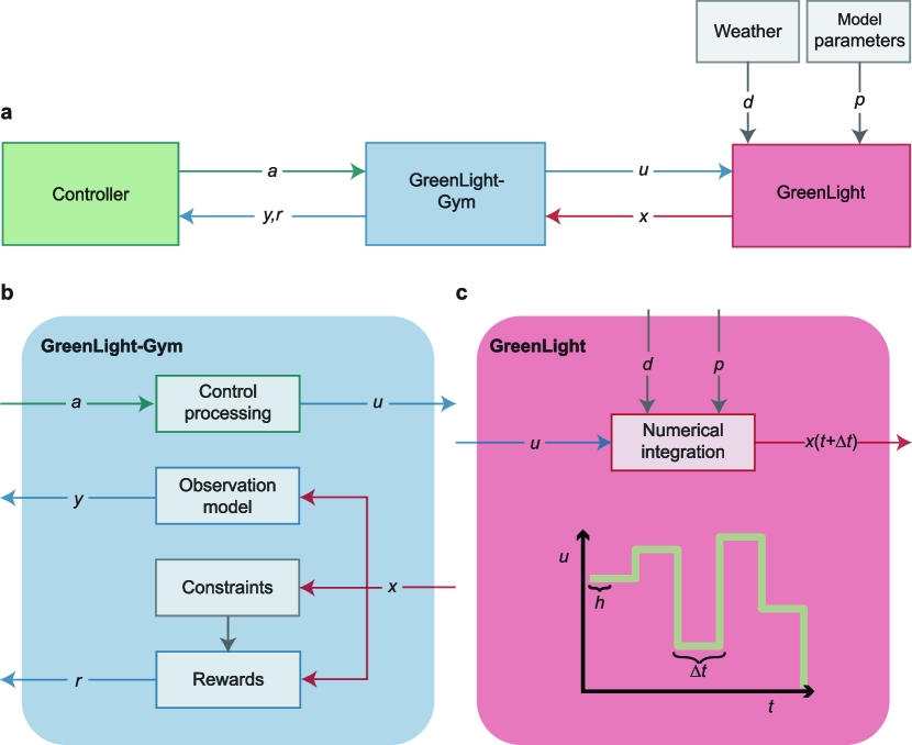
Figure 1: Representation of the GreenLight-Gym architecture. a, A controller sends an action to the environment based on system observations. The interface processes this action into a control input for the GreenLight model. Next, a numerical ODE solver uses this input with the internally simulated state, weather input and current model parameters to predict the state at the next time step $(t+\Delta t)$. b, Three modules of the interface: control processing, observations model, rewards and constraints. c, The GreenLight ODE solver estimates the next state value based on input and model parameters. The control signal is kept constant during a time step ($\Delta t$), making it a piecewise constant function.

2.5.1 Controller

The controller module within the benchmark environment is designed to support various control methods, including both learning-based and rule-based policies. This design allows users to implement and evaluate different types of controllers, providing a standardised framework for testing and comparison.

One of the primary benefits of this modular design is the ability to implement multiple RL algorithms to learn control policies. This flexibility promotes consistent progress monitoring within the learning-based greenhouse control community. The user can reliably assess the performance of various RL algorithms by using the same underlying model dynamics and weather data, along with predefined metrics.

Additionally, implementing rule-based controllers allows the user to encode general grower strategies. These rule-based controllers serve two functions: (1) as a baseline for a behavioural analysis between rule- and learning-based controllers and (2) to validate the accurate implementation of the GreenLight model in GreenLight-Gym. This comparison is crucial for verifying whether learning-based policies generate realistic control inputs. This aspect can be easily overlooked when focusing solely on the performance metrics of RL models in greenhouse crop production systems. The following key points, derived from (Katzin et al., 2021), depict the already implemented rule-based controller’s behaviour:

• Lamps $(u_{\text{lamp}})$ are on between midnight and 18.00, except when outdoor global radiation exceeds $400\text{ W m}^{-2}$, or the predicted outdoor global solar radiation sum over the day is above $10\text{ MJ m}^{-2}\text{ d}^{-1}$.

• CO₂ $(u_{\text{CO}_{2}})$ is injected during the light period whenever the concentration drops below the 800 ppm set-point. The input is computed using a P-controller.

• Heating $(u_{\text{boil}})$ is applied whenever the indoor temperature drops below the target set-point, $19.5\degree$C during the light period or $16.5\degree$C during the dark period. The heating actuator is P-controlled.

• Roof ventilation windows $(u_{\text{vent}})$ are opened whenever the indoor temperature is $5\degree$C above the target set point or if the indoor relative humidity is over 90%. Vents are closed if the indoor temperature is 1 °C below the target set point. Both ventilation incentives are P-controlled.

• Thermal screens $(u_{thscr})$ are closed if the outdoor temperature is below $5\degree$C during the day and below $10\degree$C at night. Screens are opened if the indoor temperature is $4\degree$C above the target set-point or when the indoor relative humidity is over 85%.

Note that users can define a different rule-based controller if desired.

2.5.2 Observations model

Designing observation spaces from which RL agents learn a desired control policy can be a lengthy trial-error process, making RL infeasible to conduct through real-world experimenting. Different observation spaces can seriously affect learning control policies. For instance, when observations dominate the initial learning process but are not meaningful for longer horizons (Kim and Ha, 2021). GreenLight-Gym observations module enables users to encode additional information in the observation space, defined as in (6), such as leaf area index, photosynthesis rate, or lamp intensity. The modular configuration of the observation space in GreenLight-Gym facilitates an empirical analysis of the effect of observations on approximating optimal control policies.

2.5.3 Control processing

The control processing module is designed to offer a configurable environment by defining any possible configuration of controllable greenhouse actuators, as listed in Table 2. These actuators directly manipulate the crops and indoor climate of the greenhouse, allowing for precise control over the growing conditions. Each greenhouse facility may have a unique set of actuators. The control module’s design accommodates these variations by including or excluding specific control inputs from the optimisation problem (3). This flexibility ensures that the setup can be tailored to meet the specific requirements of different greenhouse facilities.

Another notable feature of the control module is its compatibility with a hybrid control approach. This approach allows controllable inputs to be governed by a predefined rule-based strategy while a learning-based controller manages others. This hybrid approach enables users to delineate the search space for the learning-based controller, focusing on a subset of control inputs where the optimal solution is more apparent. This targeted focus makes it easier to assess the performance of the learning-based controller.

2.5.4 Rewards & constraints

In greenhouse control, a mismatch between the underlying model and the real-world system could yield high rewards in unfavourable states when purely focusing on profitability. For instance, when the negative effects of extreme humidity concentrations on crop yield and quality are neglected. Therefore, well-designed reward functions should encode the relation between costs associated with controllable input and gains from crop growth while avoiding unfavourable states that negatively affect crop growth and quality.

GreenLight-Gym’s reward & constraints module facilitates reward function design to encode desired objectives by combining one or multiple reward components that assign an immediate value to an action in a specific state. This lets users explore how greenhouse control problems translate into well-defined reward functions. In subsection 3.3.2, two reward functions are described to study how they balance profitability and constraints in the greenhouse crop production control problem.

2.5.5 Weather

Weather circumstances highly influence the system’s outcome in greenhouse crop production control. Evaluating controllers using consistent weather trajectories is essential to make a fair comparison between controllers. The weather module is designed to integrate weather data from various geographic locations and years, enabling the generation of a fixed benchmark simulation environment to assert control performance under comparable weather conditions.

GreenLight-Gym contains weather data from 2001 to 2020 recorded at a single location (Schiphol Airport) in the Netherlands. This work tests the RL agent’s capability to generalise to new weather trajectories with similar underlying distributions. Therefore, a dataset from a single location is chosen. Users are invited to include weather datasets from various locations to test the generalisation capabilities between greenhouse locations.

Prior research demonstrated the benefits of training RL-based control policies under diverse weather events. This training approach enhances the resilience of these policies against variations in weather patterns (Turchetta et al., 2022). Demonstrating the generalisation capabilities of an RL-based controller against novel weather patterns necessitates disjoint training and testing weather datasets, i.e., $(D_{\text{train}}\cap D_{\text{test}}=\emptyset)$. This setup allows the RL agent to optimise the specified objective (5) using $D_{\text{train}}$ while evaluating its performance on $D_{\text{test}}$.

2.5.6 Model parameters

GreenLight-Gym includes user-configurable model parameters that enable the specification of a wide range of greenhouse facilities and crop varieties. This allows the greenhouse control community to benchmark performance across diverse greenhouse and crop models. Moreover, prior studies indicated that training reinforcement learning RL agents across a range of model parameters, i.e., domain randomisation, enhances their ability to generalise to unseen environments (OpenAI et al., 2019; McClement et al., 2021). This is interesting since considerable parametric uncertainty exists in greenhouse crop production models, particularly in crop growth dynamics. Consequently, learning controls from diverse model parameterisations mitigates this uncertainty and improves the transferability of RL agents to real-world greenhouses.

2.5.7 Numerical solver

This work reimplements the original GreenLight model (1) into our GreenLight-Gym software architecture, tailored specifically to meet the demands of reinforcement learning models. This work adopts a fixed time-discretization approach to ensure uniform interaction intervals between the RL agent and the environment, which is essential for training and evaluating RL models. This time-discretization is achieved by implementing explicit numerical integration methods. Users can apply the fourth-order Runge-Kutta (RK4) or the first-order forward Euler method. To balance the computational efficiency required for data-intensive RL models and the precision to accurately simulate the greenhouse transition dynamics.

Since GreenLight (1) is a system of stiff ODEs, a sufficient sampling time $h$ for the numerical solver must be chosen to model its continuous behaviour accurately. Decreasing $h$ would produce a more accurate approximation of (1) but increase the program’s computational demand. Subsection 4.1 & 4.2, study the effect of the sampling time on the accuracy and execution time of the GreenLight-Gym.

3 Simulation experiments

This work conducted two simulation experiments to verify the implementation of the GreenLight-Gym environment against the original GreenLight Matlab code. In addition, three simulation studies analysed the stability and performance of an RL-based controller. This section demonstrates GreenLight-Gym’s capabilities as a software suite to train and benchmark RL-based controllers. The outline for this Section is as follows:

• In subsection 3.1 the accurate implementation of GreenLight-Gym is verified against the original Matlab implementation.

• The program’s execution time and the sensitivity of the profit-based objective and constraints regarding the control interval are examined in subsection 3.2.

• Subsection 3.3 presents a demarcated experimental setup to train two RL controllers using a different reward function. Specifically, these experiments’ simulation and training settings are detailed, as well as the metrics used for evaluation.

• Subsection 3.4 studies the sensitivity of controller performance against penalty coefficients in both controllers’ reward functions.

• Finally, subsection 3.5 evaluates controller performance for both controllers trained with different reward functions on the simulation benchmark. This benchmark consists of a disjoint weather dataset for testing. Additionally, their performance is compared against GreenLight-Gym’s rule-based controller, as described in subsection 2.5.1.

3.1 Verification of GreenLight-Gym

The first experiment verified GreenLight-Gym’s implementation against the original GreenLight Matlab code, which was validated with real-world greenhouse data (Katzin et al., 2020). By verifying the correct implementation of the model dynamics, this study demonstrates the accuracy of GreenLight-Gym for crop production control. This work employed the explicit RK4 method to approximate the behaviour of GreenLight in GreenLight-Gym. In contrast, the original Matlab implementation relies on a variable-step variable order solver (Katzin et al., 2020). This experiment tested three sampling times $h$ to balance accuracy and execution time. The simulation results for this experiment are presented in subsection 4.1.

This comparison experiment simulated twelve growth cycles of ten days each, starting on the first day of each month in 2000. Initially, the original Matlab implementation was executed with the rule-based controller described in subsection 2.5.1. The resulting states, control inputs, and disturbances were then interpolated into three different sampling intervals $h\in\{0.5,1.0,2.0\}$. Finally, GreenLight-Gym was used to simulate the same twelve periods for all three solutions. This simulation used the Matlab solution’s interpolated control inputs and weather disturbances. With the control interval set to the equivalent value as the sampling time $\Delta t=h$.

To quantitatively assess the similarity between both implementations, the relative root mean squared error (rRMSE) as follows

$$\mathrm{rRMSE}=\frac{100}{\bar{y}^{\mathrm{true}}}\sqrt{\frac{1}{n}\sum_{i=1}^{n}\left(y_{i}^{\mathrm{true}}-y_{i}^{\mathrm{pred}}\right)^{2}},$$ (8)

where $y_{i}^{\mathrm{true}}$ is the value for state $i$ from the original Matlab implementation and $y_{i}^{\mathrm{pred}}$ is the predicted value for that state from the GreenLight-Gym’s simulation.

3.2 Effect of control interval on model responsiveness

The second simulation experiment tested the relation between the control interval $(\Delta t)$ and three metrics that depict model responsiveness. Three metrics measured model responsiveness: the execution time and the sensitivity of the profit-based objective (2) and the Time Within state Boundary (TWB) per state constraint regarding the control interval. TWB was determined by the percentage of time a state constraint was violated. Larger intervals between control inputs can result in less precise control and might degrade controller performance. The rule-based controller, as described in subsection 2.5.1, computed the control input for varying $\Delta t$. The execution time was compared against the original Matlab implementation to demonstrate the balance between accuracy and runtime performance GreenLight-Gym. GreenLight’s sensitivity to the control interval $(\Delta t)$ is expected to be slightly higher than those reported in greenhouse control literature, as the employed rule-based controller calculated control inputs using a standard P-controller rather than an optimal control method (Van Beveren et al., 2015; Van Henten and Bontsema, 2008; Van Straten et al., 2000). For the results refer to subsection 4.2.

For twelve different starting dates in 2000, a control interval between 30 and 3600 seconds was simulated for ten consecutive days, complemented with the following set $\Delta t\in\{2,4,8,16\}$. The execution time was evaluated for three sampling times $h\in\{0.5,1.0,2.0\}$. The relative change in profit and TWB were computed when increasing the control interval, taking $\Delta t=2$ as a reference value. Table 3 lists the upper and lower boundaries $[\underline{\omega},\overline{\omega}]$ for three indoor climate variables.

Indoor variable	Lower bound $(\underline{\omega})$	Upper bound $(\overline{\omega})$	Unit
Temperature	10	35	°C
Carbon dioxide concentration	0	1000	ppm
Relative humidity	60	90	%

Table 3: System constraints.

3.3 Performance and stability of RL agents using two reward functions

The third simulation experiment addressed a critical challenge in reinforcement learning for greenhouse crop production: the stability and consistency of performance across different instances of trained RL-based controllers. This issue is well-recognised in reinforcement learning (Patterson et al., 2023), but often neglected in greenhouse crop production control. Our simulation experiments serve two primary purposes: (1) To present an experimental setup for controlling greenhouse crop production by managing climatic actuators with an RL-based controller and (2) to evaluate the stability and performance of two RL-based controllers trained using different reward functions, thereby assessing the impact of reward function design on learning stability and controller performance. The modular design of GreenLight-Gym facilitated this design of both the environment and controller. The results of this simulation experiment are found in subsection 4.3.

3.3.1 Simulation settings

In line with previous research (Kuijpers et al., 2021), this study focused on fully grown fruit-producing crops (generative phase). During the generative phase, the controller regularly receives feedback signals from the system during fruit growth and harvest. When the vegetative stage is considered, long optimisation horizons should be taken, and a different objective function should be designed.

To delineate the control problem, the RL-based controller managed four climate actuators. The first control input regulated the heating energy flow from the boiler to the heating pipe system $u_{\text{boil}}$. The second controlled input was the carbon dioxide injection into the greenhouse $u_{\ch{CO2}}$. The third controlled variable was the opening of the roof ventilation windows $u_{\text{vent}}$. The fourth control variable controlled the closure of the thermal screen $u_{\text{thScr}}$, preserving indoor air temperature and affecting the air exchange between the main and top air compartments. A rule-based controller managed the intensity of the LED lamps $u_{\text{lamp}}$.

The state boundaries for these experiments are described in Table 3. Indoor air temperature boundaries have a wide range as the crop model already covers the effect of non-optimal temperature regimes by inhibiting photosynthesis and its carbohydrate buffer (Vanthoor et al., 2011a). Therefore, the controller is challenged to learn these optimal patterns during training. Carbon dioxide concentration is upper bounded since this is a common saturation point for tomato crops to preserve healthy air conditions for human greenhouse operators. GreenLight does not include adverse or positive effects of humidity on crop yield and fruit quality. Therefore, relative humidity is constrained by boundaries optimal for crop growth and quality, based on existing literature (Holder and Cockshull, 1990).

3.3.2 Reward functions

This simulation experiment analysed the impact of two penalty methods on controller performance, aiming to prevent undesired controller behaviour, as discussed in the Introduction and subsection 2.5.4. The two methods evaluated are the additive penalty approach and the multiplicative penalty approach. These methods were chosen to explore their effectiveness in adjusting the reward function to enhance controller performance.

Both employed approaches consisted of two components that encode the desired controller behaviour. The first component formulated a profit-based reward function

$$r_{k}^{\text{profit}}=c^{\text{frt}}y^{\text{har}}_{k}-\sum_{i}c^{i}_{k}y^{i}_{k},$$ (9)

where $y^{\text{har}}_{k}$ is the fresh weight of harvested fruit in kg over the past time step, $c^{\text{frt}}$ is the current fruit price, $c^{i}_{k}$ denotes the current unit cost and $y^{i}_{k}$ the consumption of resource $i$ over the past time step. Table 4 describes the fixed cost coefficients for this profit-based reward function. In line with previous work, the roof ventilation and thermal screen operating costs were neglected (Kuijpers et al., 2021, 2022). This reward function assumes continuous measurements of fruit harvest. However, in reality, these measurements are observed more sparsely as fruits are approximately harvested biweekly.

Since a rule-based controller operated the lights, these costs were deliberately excluded from the reward function, focusing instead on variables directly influenced by the RL-based controller’s decisions. To stabilise the learning process, min-max scaling bounded this reward between $[0,1]$. The minimum value was defined by having no harvest and maximum resource consumption and having the maximum possible harvest without using resources defined the maximum value.

The state constraints were encoded by penalising (9) with a penalty if state boundaries were exceeded. This penalty value was calculated as the average of the normalised inverse tangent of the absolute differences between each measurement and its corresponding constraint

$$r^{\text{pen}}_{k}=\frac{1}{N_{\omega}}\sum_{i}\frac{2}{\pi}\tan^{-1}(b^{i}\Delta^{i}_{k}),$$ (10)

where $\Delta^{i}_{k}$ is the absolute difference between measurement and constraint for state $i$ at time step $k$. $b_{i}$ is a tunable coefficient that determines the steepness of the penalty curve, and $N_{\omega}$ are the number of state constraints. No penalty was given in the special case of $b^{i}=0$. This transformation bounded the penalty between $[0,1]$ for each state constraint and aligned its range with the profit reward. The inverse tangent was employed to generate a smooth and bounded penalty response, which proved more intuitive to tune via $b^{i}$ rather than directly tuning Lagrange multipliers working on $\Delta^{i}$. The penalty coefficients are shown in Table 5.

The absolute difference $\Delta^{i}_{k}$ was computed as follows

$$\Delta^{i}_{k}=\begin{cases}y^{i}_{k}-\overline{\omega}_{i}&\text{if $y^{i}_{k}>\overline{\omega}^{i}$},\\ \underline{\omega}^{i}-y^{i}_{k}&\text{if $y^{i}_{k}<\underline{\omega}^{i}$},\\ 0&\text{otherwise};\end{cases}$$ (11)

where $y^{i}_{k}$ is the $i^{\text{th}}$ state measurement, and $[\overline{\omega}^{i},\underline{\omega}^{i}]$ are the upper and lower boundaries for state variable $i$, as described in Table 3. Note that this definition of the penalty function causes discontinuity in the optimisation objective function, possibly affecting controller performance.

Two approaches were tested to encode these constraints in the final reward function. The first method subtracted the penalty function from the profit-based reward

$$r^{\mathrm{add}}_{k}=r^{\text{profit}}_{k}-r^{\text{pen}}_{k},$$ (12)

resulting in a additive penalty. The advantage of this method is the direct correlation between constraint violations and the corresponding negative impact on accumulated reward. However, a disadvantage is that the penalty can quickly dominate the objective function. This dominance could emerge due to the differing time scales on which the reward components operate. Specifically, the profit-based reward responds with a delay, as it depends on the fruit harvested at the end of the day, conditioned on optimal growth throughout the lighting period. Consequently, during periods of low profit, the penalty overtakes the objective function.

The second approach modulated the profit-based reward by multiplying the profit-based reward as follows

$$r^{\mathrm{mult}}_{k}=r^{\text{profit}}_{k}(1-r^{\text{pen}}_{k}),$$ (13)

generating a multiplicative penalty. This approach prevented the penalty function from dominating the objective function by focusing more on profit. One downside of this method was the small effect of constraint violations when the profit-based reward yielded low values.

Cost coefficients	Value	Unit	Description
$c^{\mathrm{frt}}$	$1.6$	$€/\mathrm{[FW]kg}$	Fresh weight fruit price
$c^{\mathrm{gas}}$	$0.26$	$€/\mathrm{m}^{3}$	Gas costs
$c^{\mathrm{CO}_{2}}$	$0.1$	$€/\mathrm{kg}$	$\ch{CO2}$ costs

Table 4: Values of cost coefficients of the profit-based reward function, as defined in (9).

Penalty coefficients	Value
$b^{\mathrm{T}}$	$1.2$
$b^{\ch{CO2}}$	$8.0\times 10^{-3}$
$b^{\mathrm{RH}}$	$1.0$

Table 5: Values of penalty coefficients, as defined in (10).

3.3.3 Training settings

To reflect the Dutch horticulture fruit production stage (Vermeulen, 2008), simulations started on a uniformly randomly sampled date (with replacement) between 2011 and 2020, from the first of March to the first of September. In the remainder of this work, $D_{\mathrm{train}}$ refers to this dataset. Since outdoor weather variables strongly affect greenhouse control performance, each agent sampled the simulation starting dates in the same order to make a fair comparison between the agents’ training processes. After training, the resulting controllers were evaluated on a subset of $D_{\mathrm{val}}\subset D_{\mathrm{train}}$. This subset comprised six dates in each training year (2011-2020), each starting on the first day of March to August, resulting in 60 unique episodes. Each simulation, i.e., episode, lasted ten days. The interval between control inputs was set to $\Delta t=300\mathrm{s}$ and solver sampling time to $h=1\mathrm{s}$. Training consisted of 40 million time steps resembling $\sim 13900$ episodes. Initial conditions $(x_{0})$ for indoor climate and crop states were fixed across training episodes.

For both the additive reward function (12) and multiplicative reward function (13), five controller instances were trained using the PPO algorithm to optimise (5) in order to solve the constraint optimisation problem (3). Each controller was initialised with a unique random seed yielding different initial actor and critic network parameters. This approach ensures diversity in the initial conditions and helps assess the robustness of the training process. The observation space of the agents consisted of thirteen greenhouse and five weather variables, as detailed in Table 6. The observations were normalised by calculating the mean and standard deviation at each training iteration and applying these statistics to standardise the input data. This observation space assumes continuous measurements of crop variables like fruit dry weight and harvested fruit dry weight.

The RL model used separate neural networks for actor and critic, each with three hidden layers. The actor network had 512 nodes per hidden layer, while the critic network had 1024. The Adam optimisation algorithm facilitated parameter updates within these networks, a gradient-based method known for its effectiveness in deep learning applications (Kingma and Ba, 2015). To fine-tune the PPO algorithm’s hyperparameters, a random search was conducted using the Weights and Biases platform, enabling a systematic exploration and tracking of hyperparameter impacts on model efficacy. Table 7 summarises the PPO hyperparameters informed through this random search.

Symbol	Description	Unit
$y^{\mathrm{T}}$	Indoor air temperature	°C
$y^{\ch{CO2}}$	Indoor CO2 concentration	ppm
$y^{\mathrm{RH}}$	Indoor relative humidity	%
$y^{\mathrm{CFrt}}$	Fruit dry weight	kg$/$m2
$y^{\mathrm{HarFrt}}$	Harvested fruit dry weight	kg$/$m2
$y^{\mathrm{PAR}}$	Photosynthetic Active Radiation	W$/$m2
$y^{\ch{CO2Res}}$	CO2 resource consumption	kg$/$m2
$y^{\mathrm{GasRes}}$	Gas resource consumption	kg$/$m2
$y^{\mathrm{24hCropT}}$	Daily average canopy temperature	°C
$y^{\mathrm{Hour_{sin}}}$	Sine hour of the day	-
$y^{\mathrm{Hour_{cos}}}$	Cosine hour of the day	-
$y^{\mathrm{Day_{sin}}}$	Sine day of the year	-
$y^{\mathrm{Day_{cos}}}$	Cos day of the year	-
$d^{\mathrm{iGlob}}$	Global radiation	W$/\mathrm{m}^{2}$
$d^{\mathrm{T}}$	Outdoor temperature	°C
$d^{\mathrm{RH}}$	Outdoor Relative humidity	%
$d^{\mathrm{\ch{CO2}}}$	Outdoor CO2 concentration	ppm
$d^{\mathrm{Wind}}$	Outdoor wind speed	m/s

Table 6: Observation space for the agent.

Hyperparameter	Value
Batch size	64
Number of epochs	7
Discount factor $(\gamma)$	0.99
GAE-lambda $(\lambda)$	0.995
Clip range	0.5
Entropy coefficient	0.01
Valvue function coefficient	0.5
Action layer width	512
Value layer width	1028
Adam learning rate $(\alpha)$	$7\cdot 10^{-5}$
Activation function	Sigmoid Linear Unit

Table 7: Hyperparameters for PPO algorithm.

3.3.4 Performance metrics

The stability and performance of both RL agents, using different reward functions, were analysed using two main approaches: stability assessment and controller performance. The stability assessment used the agents’ learning curves and return distributions. Controller performance was measured by the profit-based objective (2) and the Time Within state Boundaries (TWB).

The learning curve represents the episodic return averaged over the last 100 episodes. The episodic return is defined by $\sum_{k}^{N}r^{i}_{k}$, where $N$ denotes the number of time steps within a single episode and $i$ indicates the employed reward function. Episodic returns were used to directly measure cumulative performance without diminishing the importance of later rewards. Due to different reward functions, agents optimised varying objectives, making quantitative comparisons unfair. Therefore, their stability was examined through:

• Convergence rate: Computed as the gradient of the learning curve, representing how quickly each algorithm approaches its optimal performance.

• Coefficient of Variation (CV): Computed as a statistical metric of the learning curve. This metric represents the ratio of standard deviation to mean ($\mathrm{CV}=\sigma/\mu$) and indicates the relative variability during training.

• Similarity comparison: After training, both controllers were compared on $D_{\mathrm{val}}$ using a two-sided Mann-Whitney U-test (at $\alpha=0.05$) to assess the distribution of returns between controllers with different random seeds. Similar performance across seeds would confirm learning stability. Controllers achieving similar performance across random seeds confirm the stability of the learning process, as this indicates consistency despite varying initialisation of the actor and critic network.

Finally, controller performance was evaluated on weather dataset $D_{\mathrm{val}}$ using:

• Profit-based objective $r_{0:N}^{\mathrm{profit}}$ (2).

• TWB: The percentage of time state constraints are not violated. Encapsulating how well the controller handles state constraints.

These metrics facilitate a comprehensive comparison between controllers trained with different reward functions, assessing both learning stability and control performance.

3.4 Sensitivity of penalty coefficients on controller performance

The fourth experiment studied the sensitivity of the penalty coefficients on controller performance for the additive and multiplicative reward functions, as defined in (12) and (13). This study provides insight into how performance is affected by the penalty coefficients $(b^{i})$ in the two reward functions, which helps to make informed decisions on the proper setting for the reward function. It elucidates the trade-off between the two main objectives in greenhouse control: the profit-based reward objective and the state constraints. Moreover, the learning process is stable when agents show robust performance over a wide range of coefficients. These results can be found in subsection 4.4.

This experiment employed the one-factor-at-a-time approach to evaluate the sensitivity of an RL-based controller regarding individual penalty coefficients. This method involved changing one penalty coefficient $b^{i}$ while keeping others constant. For each coefficient, six values were tested over an equally spaced range per coefficient. The specific ranges are detailed in Table 8. These ranges were determined based on preliminary tests and domain knowledge to cover a meaningful spread of values.

For each set of penalty coefficients, a single RL-based controller was trained for 10 million time steps. This training duration was chosen to balance computation resources and ensure sufficient converging time for each configuration. The resulting controllers were evaluated on the profit-based objective $r_{0:N}^{\mathrm{profit}}$ and TWB per state on the evaluation dataset $D_{\mathrm{val}}$.

Penalty coefficients	Lower limit	Upper limit	Increment	Base value
$b^{\mathrm{T}}$	$0$	$2.0$	$0.4$	$1.2$
$b^{\ch{CO2}}$	$0$	$0.01$	$0.02\cdot 10^{-2}$	$0.4\cdot 10^{-2}$
$b^{\mathrm{RH}}$	$0$	$1.0$	$0.2$	$0.4$

Table 8: Values for the penalty coefficients during OAT sensitivity analysis for the penalty function, as defined in (10).

3.5 Simulation benchmark RL-based controller

The fifth and final experiment empirically analysed RL controller performance on the simulation benchmark, which consisted of 60 weather trajectories excluded during training. This experiment demonstrates the controller’s capability to generalise learned control policies to unseen weather trajectories, essential for greenhouse crop production control since true weather realisations are unknown before real-world deployment. Two trained RL-based controllers were evaluated using the additive and multiplicative reward function, (12) and (13), against the baseline rule-based controller described in subsection 2.5.1. The results for this simulation experiments are presented in subsection 4.5.

For the benchmark simulation, six dates were deliberately picked from each year between 2001 and 2010, starting on the first days of the month between March and August. This yielded 60 unique weather trajectories. In the remainder of this work, $D_{\mathrm{test}}$ refers to this dataset. Each simulation episode lasted ten days. The same initial conditions $(x_{0})$ used in training were applied to ensure comparability. It was assumed that both samples have similar distributions by sampling weather trajectories for the train and the test set from the same period throughout the year. This assumption supports a fair assessment of the generalisation capabilities of the RL-based controllers. For the training data $(D_{\mathrm{train}})$, control interval $(\Delta t)$, solver sampling time $(h)$ and initial conditions $(x_{0})$ for indoor climate and crop states is referred to subsection 3.3.3

This analysis asserted episodic return, the profit-based objective and the TWB per state constraint. Additionally, the main daily state and control input values were computed by calculating the average over every discrete time step $k$ per day in the simulation benchmark $D_{\mathrm{test}}$. This approach provides insight into the average behaviour of all three controllers. It highlights how RL-based controllers differ from general practical growing strategies regarding daily climate and crop response.

4 Results

This section presents the results of simulation experiments described in Section 3. Subsection 4.1 verifies the accurate implementation of GreenLight-Gym. Subsection 3.2 compares the execution time between the original and this study’s implementation of GreenLight. Additionally, the model’s responsibility regarding the control interval is examined. Subsection 4.3 demonstrates the results of training two RL controllers with different reward functions. Subsection 4.4 presents the controllers’ sensitivity regarding penalty coefficients. Finally, subsection 4.5 analyses controller performance on a novel benchmark test set.

4.1 Verification of GreenLight-Gym

The first simulation experiment verified the correct implementation of the GreenLight model (1) in GreenLight-Gym against the original Matlab code, as described in subsection 3.1. GreenLight-Gym employed the explicit RK4 solver and the original code a variable-step variable-order solver; hence, minor differences between the two implementations are expected. This difference is expressed by the rRMSE (8) of four state variables ($\mathrm{CO_{2,air}}$, $\mathrm{T_{air}}$, $\mathrm{VP_{air}}$, $\mathrm{C_{fruit}}$), which were computed for three sampling periods $(h(\mathrm{s})\in\{0.5,1.0,2.0\})$ seconds. Simulations that used a larger $h$ resulted in numerically unstable solutions, and a smaller $h$ was computationally infeasible. Table 9 presents the rRMSE, including their 95% confidence interval for the four mentioned state variables and sampling times averaged over twelve different simulations. For none of the state variables, significant differences were observed when changing the sampling time.

The dry weight of the fruit $(\mathrm{C_{fruit}})$ reported the lowest rRMSE of $0.02\%$ but the relatively highest confidence interval (0.02). Indoor vapour pressure and air temperature reported the highest rRMSE of $1.70\%$ and $1.45\%$, and indoor carbon dioxide concentration had an rRMSE of $0.58\%$. Physiological processes like crop growth have larger time constants, which make them less sensitive to numerical approximation errors when larger sampling times are used. Climate variables are subject to processes such as solar radiation, outdoor temperature, humidity, and ventilation, with rapid fluctuations resulting in stiff reactions with small time constants.

	State variable
$h(\mathrm{s})$ seconds	CO2, air	Tair	VPair	Cfruit
0.5	$0.58$ $(0.28)$	$1.45$ $(0.32)$	$1.70$ $(0.37)$	$0.02$ $(0.02)$
1.0	$0.57$ $(0.27)$	$1.45$ $(0.32)$	$1.71$ $(0.37)$	$0.02$ $(0.02)$
2.0	$0.57$ $(0.27)$	$1.45$ $(0.32)$	$1.70$ $(0.37)$	$0.02$ $(0.02)$

Table 9: The average relative Root Mean Squared Error (rRMSE) and 95% confidence intervals for three sampling times over twelve different simulations starting on the first day of each month in 2000.

4.2 Effect control interval

The second experiment assessed the control interval’s ($\Delta t$) effect on model responsiveness regarding execution time, profit-based objective (2) and TWB per state constraint, detailed in subsection 3.2. The execution time for GreenLight-Gym decreased as $\Delta t$ increased, see Figure 2.a. Larger control intervals corresponded to fewer computations (changes) of the control input, which caused the observed reduction in execution time, as shown in Figure 2.a. The curve of the execution time converged around $\Delta t=120$ seconds. Beyond two-minute control intervals, the reduction in execution time becomes relatively small. This suggests that other parts of the model implementation become the bottleneck, such as the sampling time $h$ of the numerical solver. The execution time demonstrated a linear relation with the sampling time, as $h$ defines the number of calculations to obtain a numerical solution. GreenLight-Gym’s model implementation gained a reduction in execution time over the original Matlab implementation by a factor of ten. The system demonstrated numerically unstable behaviour for $h=2$ and $\Delta t>100$ seconds. Therefore, the sampling remained fixed $(h=1)$ for the rest of this work to balance the accuracy and computation time, while preserving numerical stability.

Figure 2.b shows the relative change in the profit-based objective function $(r_{\text{profit}}^{T}$ as a function of $\Delta t$, for a rule-based controller. This graph shows that increasing the control interval on average decreased the profit-based objective. The reduction in $r_{\text{profit}}^{0:N}$ ranges from $0$ up to $6.6\%$. The relative change is small ($<1\%$) for $\Delta t<400$. Similar behaviour is observed in Figure 2.c, which visualises the relative change in time spent within specific state constraints. The largest drop $41.2\%$ in TWB is observed for carbon dioxide concentration, followed by humidity $11.0\%$ and air temperature $3.1\%$. The relative change in TWB destabilised slightly faster than the profit-based objective $\Delta t>300$.

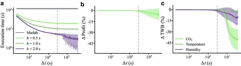
Figure 2: GreenLight-Gym’s model responsiveness regarding control interval ($\Delta t$). The dashed grey line represents this study’s chosen control interval $\Delta t=300$. a, Execution time plotted as a function of $\Delta t$ for GreenLight-Gym for three different sampling times $h$. The execution time for Matlab is invariant to the control interval, as no fixed interval is defined. b, Relative change in $r^{\mathrm{profit}}_{0:N}$ for varying control intervals. Using $\Delta t=2$ as a reference. c, Relative change in the Time Within state Boundary (TWB) for three indoor state variables. Using $\Delta t=2$ as a reference.

4.3 Performance and stability of RL controllers using different reward functions

The third experiment assessed the training stability and performance of two RL controllers trained using the additive and the multiplicative penalty approach (12) and (13), as outlined in subsection 3.3. Both controllers rapidly improved performance over the first 10 million time steps, as seen in the sharp initial rise in Figure 3.a. During the final 30 million time steps, the increments in performance were relatively small, around $3\%$. The low CV, in Figure3.c, of the learning curve indicates a stable learning process across RL controllers that were initialised with different random seeds. After 10 million time steps, the CV for both methods further decreases with standard deviations remaining below $2\%$ of the mean.

Although both controllers were demonstrating similar learning behaviour, differences emerged. The additive penalty yielded a lower episodic return than the multiplicative penalty approach. This naturally results from subtracting an absolute penalty value from the profit-based reward (9), which generates a range of $[-1,1]$ for the reward function. In contrast, the multiplicative penalty modulated the profit-based reward, reducing the penalising effect at low-profit values, generating a range of $[0,1]$. Interestingly, the additive penalty controller approached the episodic return of the multiplicative reward controller. This is illustrated by the decreasing difference between both controllers: $4.15\%$ after 9 million time steps and $1.37\%$ after 40 million time steps, suggesting higher asymptotic performance for the additive penalty approach.

Figure 3.b shows the convergence rates of both learning curves, where increments in the learning curve over millions of time steps result in minimal changes. This makes it hard to observe these small differences in learning behaviour in the convergence rate. Both controllers exhibited similar oscillatory behaviour during training. Behaviour reflected due to the random sampling of weather trajectories, affecting performance, as discussed in subsection 3.3. Note that for the first 10 million time steps, the logarithmic scale of the x-axis mitigates the appearance of these fluctuations.

To analyse the similarity of the RL controllers across different random seeds, their resulting controllers were evaluated on $D_{\mathrm{val}}$. The distributions of the episodic return in Figure 3.d show minor differences for the controllers trained using the additive penalty function, indicating low variability. In contrast, the multiplicative approach exhibits more variability. The Mann-Whitney U-test $(\alpha<.05)$ supports this observation, showing no significant differences between the episodic returns of the controllers with an additive penalty. In contrast, three out of ten controller pairs significantly differ when trained with the multiplicative penalty. See Table 10 for the detailed test outcomes.

Further analysis of the underlying metrics reveals two key findings. First, controllers trained with the multiplicative penalty performed better in terms of the profit-based objective (2), as seen in Figure 3.e. This approach focused more on the profit-based objective by modulating the profit-based reward instead of directly penalising it. The average profit per growth cycle across random seeds ranged between $3.80$ and $3.99(\mathrm{{€\,}/m^{2}})$ for the multiplicative approach, compared to $3.70$ and $3.83(\mathrm{{€\,}/m^{2}})$ for the additive approach. Second, this focus on profit resulted in a lower percentage of TWB for the multiplicative controller, particularly for relative humidity, as observed in Figure 3.f. The TWB for relative humidity ranged between $62.7\%$ and $72.0\%$ for the multiplicative approach, compared to $84.9\%$ and $89.6\%$ for the additive approach. Both methods effectively managed the state boundaries for $\ch{CO2}$ concentration and temperature.

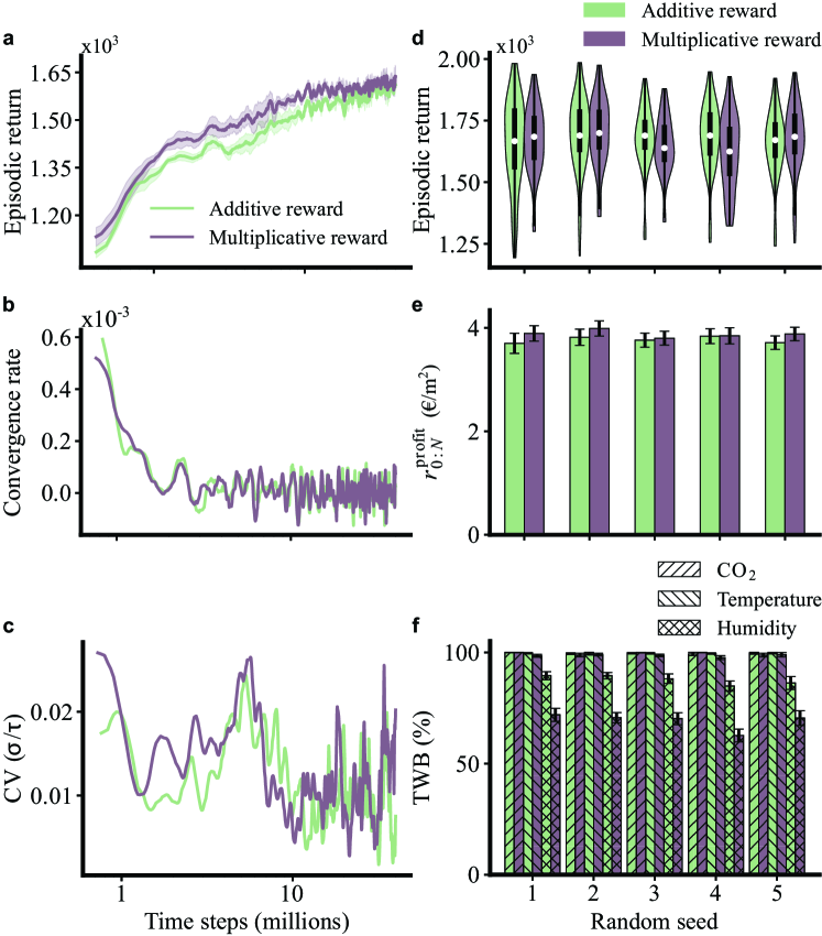
Figure 3: Analysis of training stability and performance of both RL controllers trained with different reward functions. The left figures visualise the RL controller stability during the training process. Note the logarithmic scale on the x-axis. Figures d-f show the performance metrics of the resulting controllers evaluated on $D_{\mathrm{val}}$. a, Visualises the learning curve of both RL controllers by plotting the average episodic return over the last 100 episodes during the training. The curve represents the mean value and standard deviation of five instances of the RL controller initiated with different random seeds. b, The convergence rate of both controllers trained with different reward functions was calculated by taking the gradient of the learning curve. c, Coefficient of variation (CV) of the learning curve, which represents the ratio between the standard deviation and the mean. d, Distribution of the episodic return for each RL controller initialised with a different random seed. e, Mean value of profit-based objective (2) with their $95\%$ confidence interval for each RL controller initiated with a different random seed. Evaluated on $D_{\mathrm{val}}$ f, Visualising the average percentage of Time Within state Boundaries (TWB) with their $95\%$ confidence interval for three indoor state variables for each randomly initiated RL controller.

Seed 1	Seed 2	Additive reward	Multiplicative reward
1	2	1611 (0.322)	1533 (0.162)
1	3	1730 (0.715)	2041 (0.207)
1	4	1682 (0.537)	2151 (0.066)
1	5	1871 (0.711)	1737 (0.743)
2	3	1950 (0.433)	2298 (0.0.009)
2	4	1893 (0.637)	2374 (0.003)
2	5	2130 (0.084)	2014.0 (0.262)
3	4	1728 (0.707)	1953 (0.394)
3	5	1987 (0.328)	1469 (0.083)
4	5	2064 (0.167)	1411 (0.0414)

Table 10: Mann-Whitney U-test for comparing the episodic return between random seeds. Results of the two-sided Mann-Whitney U-test comparisons between RL controllers initialised with different random seeds (U-statistic (p-value)) when evaluated on $D_{\mathrm{val}}$. The third column shows the test results for the additive penalty method, while the fourth column shows the results for the multiplicative penalty method. Bold statistics indicate significant differences in the distribution of the episodic returns between corresponding controllers with different random seeds. The episodic returns are visualised in Figure 3.d.

4.4 Sensitivity of penalty coefficients on controller performance

A sensitivity analysis was conducted to evaluate the impact of penalty coefficients in (10) on controller performance, as described in subsection 3.4. This provides insight into the robustness of RL controllers trained with either the additive or the multiplicative penalty regarding these coefficients. As shown in Figure 4.a, setting the penalty coefficient to zero $b^{i}=0$ for state $i$ generally decreased the TWB for that state boundaries. This indicates more frequent constraint violations. This trend was consistent across all indoor climate variables except for indoor temperature.

The deviating behaviour of indoor temperature, observed in the middle graph of Figure 4.a can be attributed to two potential factors. First, the crop model inhibits fruit growth outside of optimal canopy temperature ranges (Vanthoor et al., 2011a). This model assumption incentivises the controller to maintain the greenhouse temperature within this range in order to optimise fruit growth conditions and maximise the profitability (2). Second, the relatively wide range of temperature constraints naturally results in less frequent violations compared to other state variables, making the controllers less sensitive to the impact of this particular penalty coefficient.

Figure 4.a revealed that the TWB performance for both controllers was most sensitive to the penalty coefficients for relative humidity. Completely removing the relative humidity constraint $(b_{\mathrm{RH}}=0)$ significantly lowered TWB for both controllers. This outcome aligns with the model assumptions, as the employed crop model does not capture positive or negative humidity effects on crop yield and quality. Thus, without an explicit penalty, the controllers had no incentive to maintain relative humidity within bounds. Interestingly, the additive penalty approach demonstrated an amplified sensitivity regarding changes in the relative humidity coefficient $(b_{\mathrm{RH}})$ compared to the multiplicative penalty approach. The controller trained with the additive penalty showed a rapid increase in TWB as $b_{\mathrm{RH}}$ increased. Stabilising at approximately $90\%$ as $b_{\mathrm{RH}}\geq 0.4$. In contrast, the controller trained with the multiplicative penalty reached a lower asymptotic performance at approximately $66\%$. A comparable pattern emerged for the constraints on $\ch{CO2}$ concentration. The lower TWB observed for the multiplicative penalty can be attributed to its approach of modulating the profit-based reward function with the penalty-based reward (10). This modulation only significantly affects the reward function when the profit-based reward yields high values, such as during daytime hours when fruit harvest is high. Consequently, the multiplicative penalty approach may not enforce constraints as strictly during periods of lower profitability.

The sensitivity analysis also revealed significant differences in how penalty coefficients affected profit performance between the multiplicative and additive penalty approaches. As illustrated in Figure 4b, varying penalty coefficients of the multiplicative penalty approach had minimal impact on its profit performance. This robustness in profitability aligns with the multiplicative penalty design, which emphasises the profit-based reward component. In contrast, the additive penalty approach showed a larger impact on profit, as, in general, larger penalty coefficients resulted in lower profits. This outcome was expected as the additive penalty could dominate the reward function, resulting in more conservatism at the expense of profits. However, when the penalty for indoor temperature constraints was removed, $(b_{\mathrm{T}}=0)$ from the reward function, the controller trained with the additive penalty slightly degraded in profitability. A counterintuitive result since fewer constraints typically emphasise the profit-based objective. This finding suggests that the additive penalty controller struggles to learn the long-term modelled relation between optimal canopy temperatures and fruit growth.

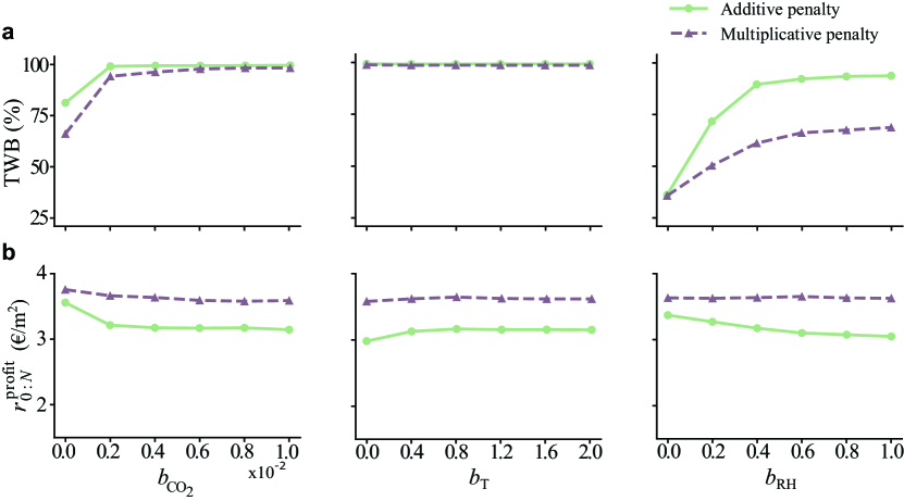
Figure 4: Sensitivity analysis of penalty coefficients on controller performance. Each point represents the performance on the benchmark test set for CO₂, temperature and relative humidity, from left to right for a specific set of penalty coefficients. One coefficient at a time is changed while the others remain fixed. a, The average Time Within state Boundaries (TWB) per state. b, The average realised profit (2).

4.5 Benchmark RL for crop production control

The fifth and final experiment analysed the performance of the RL and rule-based controllers on the simulation benchmark, which consists of 60 weather trajectories that were excluded during training, as detailed in subsection 3.5. Table 11 lists the average performance of all three controllers. As expected, both RL-based controllers decrease their episodic return when evaluated on unseen weather data. Analysing the underlying metrics of the episodic return reveals that the degraded performance is mainly driven by a decrease in the profit-based objective (2), while the controllers maintain similar performance regarding state constraints across both datasets. The decrease in profit can result from two sources. First, the weather trajectories in $D_{\mathrm{test}}$ might be less favourable for fruit yield with minimal operational costs, i.e., heating and CO2 injection. The $2.2\%$ decrease in profit for the rule-based controller supports this cause. Second, the RL controllers could suffer some degradation in performance due to unseen weather patterns, causing them to compute suboptimal controls.

Controller	Train $(D_{\mathrm{val}})$				Test $(D_{\mathrm{test}})$
	Return	$r_{0:N}^{\text{profit}}$	TWB${}_{\ch{CO2}}$	TWBT	TWBRH	Return	$r_{0:N}^{\text{profit}}$	TWB${}_{\ch{CO2}}$	TWBT	TWBRH
Additive	1696.5	3.82	99.5	99.5	89.6	1663.0	3.71	99.7	99.7	88.2
Multiplicative	1706.1	3.99	98.9	99.1	70.7	1681.7	3.91	99.5	99.4	70.4
Rule-based	-	3.97	99.9	99.9	83.1	-	3.88	99.9	99.9	84.1

Table 11: Train and test performance of RL and rule-based controllers using different penalty methods. The resulting RL controllers and the rule-based controller, as described in subsection 2.5.1, were evaluated on both $D_{\mathrm{val}}$ and $D_{\mathrm{test}}$. The recorded performance metrics were episodic return, the profit-based objective (2), and the TWB for three indoor climate variables. Since the rule-based controller did not use an underlying reward function, no episodic return was reported. The reported values represent the average over all 60 simulations in both sets.

In Figure 5, the best-performing RL controllers and the rule-based controller on $D_{\mathrm{test}}$ are compared. A Mann-Whitney U-test was performed to evaluate whether controller performance differed in terms of profit. The RL controller trained using the multiplicative penalty had significantly higher profits $(3.97\pm 0.11{€\,}/\mathrm{m^{2}})$ than the controller using the additive penalty $(3.83\pm 0.11{€\,}/\mathrm{m^{2}})$ $(p=0.007)$. No significant differences in profitability were found between either the multiplicative penalty controllers and the rule-based controller $(3.88\pm 0.15{€\,}/\mathrm{m^{2}})$ $(p=0.534)$ or the additive penalty controller $(p=0.056)$. Figure 5.b shows the TWB for all three controllers. Contrasting the results on profits, the RL controller trained with the additive penalty outperformed the RL controller using the multiplicative penalty in terms of TWB. In particular, the relative humidity constraint was maintained significantly more accurately at $87.9\pm 3.2\%$ at $70.9\pm 3.4\%$.

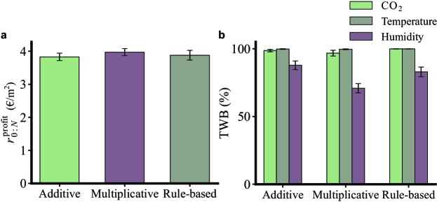
Figure 5: Average performance of the RL-based and rule-based controllers when evaluated on $D_{\text{test}}$. a, Mean value of profit-based objective on (3) with their $99\%$ confidence intervals. b, Visualising the average percentage of Time Within state Boundaries (TWB) with their $99\%$ confidence intervals for three indoor state variables.

Figure 6.a-d visualises the average daily state trajectory for indoor air temperature, carbon dioxide concentration, relative humidity and the daily cumulative fruit harvest to further analyse how the reported performance differences between controllers emerged. Interestingly, both RL controllers steered on much lower CO2 levels throughout the day compared to the rule-based controller. Despite the decreased carbon dioxide concentrations, the loss in terms of accumulated fruit harvest was small $(0.013$ $\mathrm{kg/m^{2}})$. Moreover, the multiplicative penalty approach managed lower indoor temperatures, especially near the end and the start of the day. Resulting in higher profits observed in Figure 5.a. Figure 6.c shows that the multiplicative penalty controller had an elevated relative humidity at the start of the day, exceeding the state constraint of $90\%$, declaring the decreased performance regarding TWB for relative humidity for this controller. The multiplicative controller steered the latter two indoor climate variables distinctively during the start of the day due to its underlying reward function. Modulating the profit-based reward by the multiplicative penalty removed the incentive to maintain state boundaries when the environment yields low profit, for instance, during the first hours of the day.

Figure 7.a-d visualises the average daily control input. The multiplicative penalty controller actuated the boiler and injected CO2 with the lowest intensity compared to the other controllers, confirming its optimisation for profits by minimising costs. RL-based controllers actively used the roof ventilation and thermal screen to steer the indoor climate. Likely, since the latter two have no direct cost in the profit-based reward function (9).

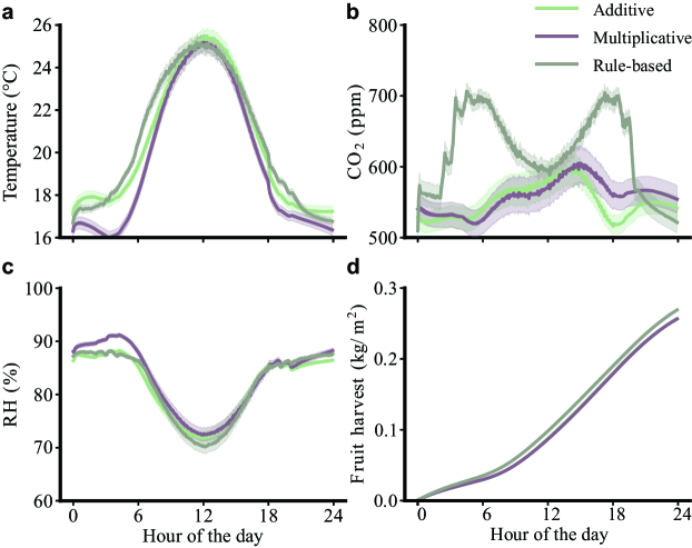
Figure 6: Average daily state trajectory. Each graph plots the average state variable for all three evaluated controllers over the day. The graphs plot the average value taken over all the days in $D_{\mathrm{test}}$, i.e., 600 days, including their $99\%$ confidence interval. a, Indoor air temperature. b, Indoor carbon dioxide concentration. c, Indoor relative humidity. d, Cumulative fruit harvest.

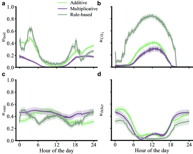
Figure 7: Average daily controls. Each graph plots the average control input over the day for the RL and the rule-based controllers. The y-axis represents relative values. The average was taken over all the days in $D_{\text{train}}$, i.e., 600 days, including their $99\%$ confidence interval. a, Valve opening from boiler to heating pipes. b, CO2 injection. c, Roof ventilation aperture. d, Closure of the thermal screen.

5 Discussion

This section discusses the main outcomes of this study, which are twofold: (1) GreenLight-Gym as a benchmark environment for training and testing RL algorithms to control greenhouse crop production systems. This includes the verification of the GreenLight-Gym (Python) against the original GreenLight (Matlab) implementation and analysing its execution time and model responsiveness, as shown in subsections 4.1 & 4.2. (2) The results of the simulation experiments regarding RL controllers, which demonstrated the capabilities of GreenLight-Gym by testing the effect of different reward functions on controller behaviour, as presented in subsections 4.3, 4.4 & 4.5.

5.1 GreenLight-Gym as benchmark environment for RL

GreenLight-Gym reimplemented the state-of-the-art GreenLight model (Katzin et al., 2020), tailored for training RL controllers through a user-friendly interface for interactions between GreenLight-Gym and RL controllers. Additionally, the model was optimised for execution time. This open-source software functions as a benchmark environment for monitoring, tracking and comparing the progress of RL control algorithms for greenhouse crop production.

In contrast to extensively studied advanced control methods, such as MPC, RL agents approximate the controller before deployment. This allows them to learn from many scenarios upfront, using complex models that accurately capture real-world dynamics. The original GreenLight model empirically demonstrated its accuracy for capturing indoor climate dynamics (Katzin et al., 2020). However, the employed crop models still rely on assumptions. This could result in unrealistic profits in some states due to unmodelled effects on crop growth and quality. However, when steered within climatic boundaries for which the crop model was validated (Vanthoor et al., 2011a), GreenLight-Gym is considered sufficiently accurate for serving as a benchmark environment for training RL controllers or testing any other controller.

5.1.1 Verification of GreenLight-Gym

GreenLight-Gym’s state dynamics were verified against GreenLight’s original Matlab implementation. Since this Matlab solution has been validated against real-world greenhouse data, it suffices to verify GreenLight-Gym against GreenLight so that the environment is suitable as a benchmark for (RL) control of greenhouse crop production systems.

The presented results in subsection 4.1 demonstrate that GreenLight-Gym’s model implementation matches the original Matlab solution. The largest differences, as shown in Table 9, arise from the fast physical processes for the indoor climate variables. As GreenLight is a system of stiff ODEs, an accurate approximation of the continuous dynamics requires sufficient low sampling times $(h)$ to meet the fast time constants of physical processes. The chosen sampling times were sufficient to attain numerically stable solutions. The small differences in rRMSE result from the fixed $h$ of GreenLight-Gym’s solver, which is required by the employed numerical solver, as outlined in subsection 2.5.7. This might, for some time instances, be not small enough and consequently match the time constants of the physical processes. In contrast, the original Matlab solution uses a variable-step solver to meet these time constants during rapid fluctuations in state variables. In conclusion, the approximation errors were sufficiently small $(<2\%)$ to serve as a benchmark environment for RL control of greenhouse crop production systems.

5.1.2 Relation control interval and model responsiveness

The results in subsection 4.2 show that GreenLight-Gym, compared to GreenLight’s original Matlab code, reduced the execution time on average by a factor of ten for a ten-day simulation. Sampling time $h$ demonstrates a linear relation with execution time, as shown in Figure 2.a. Larger sampling times resulted in numerically unstable behaviour for larger control intervals $(\Delta t>100)$.

The simulation results, as detailed in subsection 2.5.1, revealed a significant degradation in the rule-based controller’s performance when control intervals exceeded five minutes ($\Delta t>300$ s). This outcome was unexpected since the characteristic time scale of the greenhouse climate is in the order of fifteen minutes to one hour (Van Straten et al., 2000). Moreover, previous simulation studies demonstrated that the relation between energy consumption and the control interval of an optimally controlled greenhouse is stable up to a control resolution of 30 minutes (Van Beveren et al., 2015; Van Henten and Bontsema, 2008). One potential explanation for this observed discrepancy with the literature is the nature of the rule-based P-controller employed in this simulation experiment. This P-controller exhibits suboptimal behaviour and may not adequately respond to dynamic greenhouse conditions. An effect that amplifies when control intervals increase. The control interval was fixed to a five-minute frequency to maintain a fair comparison between the rule-based and RL controllers in future experiments.

5.2 Simulation experiments regarding RL controllers

This subsection discusses the simulation experiments that studied the effect of imposing state constraints on RL controllers via the reward function on controller performance. RL offers promising capabilities for greenhouse control. However, it is important to acknowledge certain limitations in its framework. The discount factor, for instance, is primarily a mathematical construct. It facilitates the convergence of RL models to numerical solutions over infinite optimisation horizons rather than accurately representing the real-world greenhouse optimisation problem (3). Despite this mathematical assumption, RL controllers can find solutions to the greenhouse control problem, as expected from previous RL applications to complex control tasks Bellemare et al. (2020); Wurman et al. (2022); Degrave et al. (2022).

5.2.1 Performance and stability of training RL controllers

The effect of two different penalty approaches on RL controller stability and performance was tested: the additive penalty (12) and the multiplicative penalty (13). The episodic return of both RL controllers trained with two penalty methods demonstrates a similar pattern in the learning curve, as visualised in Figure 3.a. Emphasised by the identical fluctuations in the convergence rate, as shown in Figure 3.b. These fluctuations result from training on a broad set of weather trajectories spanning ten years $(2011-2020)$. This work is the first to train RL controllers for greenhouse crop production control on an openly available weather dataset spanning such a large period.

The asymptotic performance of the additive penalty approach seems higher as it approaches the performance of the controller using the multiplicative penalty. Contrasting Bellemare et al. (2020) who reported that additive penalties could dominate RL’s objective function (5). This result might be an effect of the more complex relation between exceeding state boundaries and the reward of the multiplicative approach. Modulating the profit-based reward through a multiplicative penalty has little effect during low profit-based values. However, these profit-based values vary hourly, e.g., between dark and light periods and seasonally. Since the weather trajectories span multiple months throughout the year, this impacts the learning process for the multiplicative approach more than the additive approach. This probably also impacted the consistency of the multiplicative approach, as shown in Table 10.

Imposing state constraints through the reward function causes discontinuities in the objective function, which affects controller behaviour and performance. The presented results in subsection 4.3 imply larger impacts on the multiplicative penalty rather than the additive penalty method. However, in line with the literature on applied RL, penalising undesired behaviour via the reward function causes RL to solve complex control tasks (Bellemare et al., 2020; Degrave et al., 2022; Wurman et al., 2022).

Given a sampled weather trajectory, the system’s current state and control input, GreenLight-Gym modelled deterministic greenhouse crop production dynamics, assuming perfect predictions of the dynamics and knowledge of the measurements. However, in practice, uncertainties exist in the greenhouse crop production systems. Crop growth dynamics can differ due to uncertainty regarding model parameters. Additionally, observations for RL controllers come from sensory measurements with limited accuracy, resulting in errors and uncertainties. RL controller performance should, therefore, be seen as the optimal performance that can be achieved given the current training setup (model). The advantage of this deterministic modelling approach is that these uncertainties do not blur the observed results regarding training stability across random seeds and weather trajectories.

This study assumed fully-grown fruit-producing crops (generative phase), as mentioned in subsection 3.3. Therefore, the presented results only reflect this crop growth stage. During the vegetative phase, resource costs are not balanced by fruit growth, yielding sparse and delayed rewards. The current design of the reward function would require long-term optimisation horizons to capture the trade-off between resource consumption during the vegetative phase and future fruit yield. In that case, RL controllers require temporal abstraction to learn relations between state-action pairs during the vegetative phase and (delayed) future rewards, for example, through hierarchical RL (Vezhnevets et al., 2017).

5.2.2 Sensitivity of penalty coefficients on controller performance

Within certain ranges, both penalty approaches demonstrate robust performance regarding variation in the penalty coefficients in (10), shown by the results presented in subsection 4.4. The constraint on indoor temperature demonstrates the least sensitivity to its coefficient value. Since the employed crop model has optimal temperature regimes for fruit growth, this constraint is met regardless of the penalty coefficient. The inverse holds for relative humidity. This outcome results from unmodelled positive and negative effects of humidity on fruit growth and quality. Suppose future models can capture all the positive and negative relations between indoor climate variables and crop growth and quality. Then, these results suggest that state constraints imposed on RL controllers could be removed in that case.

The multiplicative penalty approach demonstrates very low sensitivity regarding the profit-based objective, as seen in Figure 4.b. This stems from the design of the multiplicative penalty function, which emphasises the profit-based reward component. However, it comes at the cost of constraint violations since the TWB for relative humidity significantly underperforms compared to the additive penalty approach.

This work shows that penalising reward functions to impose desired behaviour is a viable approach to obtaining reasonable solutions to the greenhouse control problem. On the contrary, this approach requires tuned coefficients to balance the trade-off between profitability and constraint minimisation. Previous works showed the viability of this approach (Degrave et al., 2022; Wurman et al., 2022). However, in an ideal world, the reward function encodes simply what the controller must achieve rather than how it should be achieved (Sutton and Barto, 2018). A viable method to define such a reward function while satisfying state constraints could be IPO (Liu et al., 2020).

5.2.3 Benchmark RL for crop production control

The results presented in subsection 4.3 reported controller performance on a subset of the training dataset. In practice, weather trajectories during deployment in a real-world greenhouse are unknown. Therefore, to ensure a fair assessment of performance, the RL controllers’ generalisation capabilities to unseen weather trajectories are asserted by comparing controller performance on the train and test set. Table 11 shows that both RL controllers generalise to unseen weather trajectories, with minor performance degradation in profitability. This comparison assumes similar distributions of weather trajectories across the train and test set. The rule-based controller demonstrates that this assumption does not completely hold since the test set demonstrates slightly less favourable weather for efficient fruit yield. However, the similarities between the changes in performance for RL controllers and rule-based controllers suggest that both RL methods generalise their controllers to unseen weather trajectories. This work was the first to address the generalisation of RL controllers regarding unseen weather trajectories in greenhouse crop production control. Nevertheless, the results are similar to other RL simulation experiments in the agricultural domain (Turchetta et al., 2022).

As observed in Figures 3.e-f & 5, the multiplicative penalty approach performs best regarding the profit-based objective. However, it struggles with adhering to imposed state boundaries, especially for relative humidity. These differences in performance become clear from the state and control input trajectories in Figures 6 & 7. During the first hours of the day, relative humidity exceeds the state boundary. During these moments of the day, the effect of modulating the profit-based reward with a multiplicative penalty is too low.

6 Conclusion and future work

This work introduces GreenLight-Gym, a benchmark environment for training and testing reinforcement learning (RL) controllers in greenhouse crop production systems. GreenLight-Gym’s modular design and optimised execution time facilitate rapid iteration in RL controller development, enabling focused studies on specific aspects such as reward function design and controller performance under varied weather conditions. GreenLight-Gym, a reimplementation of the process-based GreenLight model, was verified by comparing its state dynamics against the original Matlab implementation. This demonstrated its reliability as an RL benchmark environment for greenhouse crop production control.

Three simulation experiments evaluated the stability, performance, and behaviour of RL controllers when imposing state constraints by penalising their reward function. The experiments compared the additive and multiplicative penalty approaches. The additive approach showed more consistent behaviour across random seeds and seemed to have higher asymptotic performance, while the multiplicative approach prioritised profits at the cost of constraint violations. Imposing state constraints through the reward function required balancing the trade-off between profits and state constraints via penalty coefficients in the reward function. The multiplicative penalty approach is deemed less sensitive to these coefficients but again at the cost of constraint violations.

In conclusion, due to the significantly fewer constraint violations and the potential higher asymptotic performance of the episodic return, the additive penalty approach is the better method for imposing state constraints by penalising the reward function for greenhouse control. Importantly, both RL controllers demonstrated the ability to generalise their learned control policies to unseen weather trajectories. The rule-based controller evidenced that the slight drop in profitability of both RL controllers was attributable to less favourable weather conditions. These results suggest that the proposed RL controllers can handle uncertainties from unseen weather conditions, making them reliable for real-world deployment.

This work used the deterministic GreenLight model. Real-world greenhouse systems involve uncertainties in both state dynamics and measurements. Currently, the effect of these uncertainties on RL controller performance in greenhouse systems is unknown. Future research should investigate the impact of these uncertainties. Techniques such as domain randomisation and meta-RL could be explored to enhance controller robustness against these uncertainties. Another area for future research is the relationship between the vegetative and the generative phase of crop growth. The current literature lacks studies on the temporal relation between balancing resource consumption during the vegetative phase and fruit yield during the generative phase. Hierarchical RL could address this long-term optimisation challenge. Finally, future work could explore constraint policy optimisation methods for satisfying state constraints. These methods could eliminate manual tuning of the balance between state constraints and profitability, leading to more reliable controllers. GreenLight-Gym provides a modular platform for these proposed studies. Facilitating the progress in learning-based control for greenhouse crop production systems.

Data availability

The code repository to reproduce the presented results is available on https://github.com/BartvLaatum/GreenLightGym. This repository is an open-source project facilitating the development of autonomous greenhouse climate control using learning-based methods.

Declaration of competing interest

The authors declare that they have no known competing financial interests or personal relationships that could have appeared to influence the work reported in this paper.

Funding sources

This work has been funded by the Sector Plan for Science and Technology established by the Dutch Ministry of Education, Culture and Science.

References

- Abbasi et al. (2022) Abbasi, R., Martinez, P., Ahmad, R., 2022. The digitization of agricultural industry – a systematic literature review on agriculture 4.0. Smart Agricultural Technology 2, 100042. doi:10.1016/j.atech.2022.100042.
- Achiam et al. (2017) Achiam, J., Held, D., Tamar, A., Abbeel, P., 2017. Constrained Policy Optimization. arXiv preprint arXiv:1705.10528.
- An et al. (2021) An, Z., Cao, X., Yao, Y., Zhang, W., Li, L., Wang, Y., Guo, S., Luo, D., 2021. A Simulator-based Planning Framework for Optimizing Autonomous Greenhouse Control Strategy. Proceedings of the International Conference on Automated Planning and Scheduling 31, 436--444. doi:10.1609/icaps.v31i1.15989.
- Bellemare et al. (2020) Bellemare, M.G., Candido, S., Castro, P.S., Gong, J., Machado, M.C., Moitra, S., Ponda, S.S., Wang, Z., 2020. Autonomous navigation of stratospheric balloons using reinforcement learning. Nature 588, 77--82. doi:10.1038/s41586-020-2939-8.
- Boersma et al. (2022) Boersma, S., Sun, C., van Mourik, S., 2022. Robust sample-based model predictive control of a greenhouse system with parametric uncertainty, in: IFAC-PapersOnLine, pp. 177--182. doi:10.1016/j.ifacol.2022.11.135.
- Bohez et al. (2019) Bohez, S., Abdolmaleki, A., Neunert, M., Buchli, J., Heess, N., Hadsell, R., 2019. Value constrained model-free continuous control. doi:10.48550/arXiv.1902.04623, arXiv preprint arXiv:1902.04623.
- Cao et al. (2022) Cao, X., Yao, Y., Li, L., Zhang, W., An, Z., Zhang, Z., Xiao, L., Guo, S., Cao, X., Wu, M., Luo, D., 2022. IGrow: A Smart Agriculture Solution to Autonomous Greenhouse Control, in: Proceedings of the AAAI Conference on Artificial Intelligence, pp. 11837--11845. doi:10.1609/aaai.v36i11.21440, arXiv preprint arXiv:2107.05464.
- Chow et al. (2017) Chow, Y., Ghavamzadeh, M., Janson, L., Pavone, M., 2017. Risk-Constrained Reinforcement Learning with Percentile Risk Criteria. arXiv preprint arXiv:1512.01629.
- De Ruyter et al. (2021) De Ruyter, J., Menkveld, N., Leguijt, M., 2021. Glasgroenten: van efficiëntie naar waarde. Technical Report. ABN AMRO. Amsterdam.
- Degrave et al. (2022) Degrave, J., Felici, F., Buchli, J., Neunert, M., Tracey, B., Carpanese, F., Ewalds, T., Hafner, R., Abdolmaleki, A., De Las Casas, D., Donner, C., Fritz, L., Galperti, C., Huber, A., Keeling, J., Tsimpoukelli, M., Kay, J., Merle, A., Moret, J.M., Noury, S., Pesamosca, F., Pfau, D., Sauter, O., Sommariva, C., Coda, S., Duval, B., Fasoli, A., Kohli, P., Kavukcuoglu, K., Hassabis, D., Riedmiller, M., 2022. Magnetic control of tokamak plasmas through deep reinforcement learning. Nature 602, 414--419. doi:10.1038/s41586-021-04301-9.
- Dulac-Arnold et al. (2021) Dulac-Arnold, G., Levine, N., Mankowitz, D.J., Li, J., Paduraru, C., Gowal, S., Hester, T., 2021. Challenges of real-world reinforcement learning: Definitions, benchmarks and analysis. Machine Learning 110, 2419--2468. doi:10.1007/s10994-021-05961-4.
- FAO (2022) FAO, 2022. The Future of Food and Agriculture -- Drivers and Triggers for Transformation. Number 3 in The Future of Food and Agriculture, FAO, Rome.
- Holder and Cockshull (1990) Holder, R., Cockshull, K.E., 1990. Effects of humidity on the growth and yield of glasshouse tomatoes. Journal of Horticultural Science 65, 31--39. doi:10.1080/00221589.1990.11516025.
- Iddio et al. (2020) Iddio, E., Wang, L., Thomas, Y., McMorrow, G., Denzer, A., 2020. Energy efficient operation and modeling for greenhouses: A literature review. Renewable and Sustainable Energy Reviews 117, 109480. doi:10.1016/j.rser.2019.109480.
- Katzin et al. (2021) Katzin, D., Marcelis, L.F., Van Mourik, S., 2021. Energy savings in greenhouses by transition from high-pressure sodium to LED lighting. Applied Energy 281, 116019. doi:10.1016/j.apenergy.2020.116019.
- Katzin et al. (2020) Katzin, D., Van Mourik, S., Kempkes, F., Van Henten, E.J., 2020. GreenLight -- An open source model for greenhouses with supplemental lighting: Evaluation of heat requirements under LED and HPS lamps. Biosystems Engineering 194, 61--81. doi:10.1016/j.biosystemseng.2020.03.010.
- Kaufmann et al. (2023) Kaufmann, E., Bauersfeld, L., Loquercio, A., Müller, M., Koltun, V., Scaramuzza, D., 2023. Champion-level drone racing using deep reinforcement learning. Nature 620, 982--987. doi:10.1038/s41586-023-06419-4.
- Kim and Ha (2021) Kim, J.T., Ha, S., 2021. Observation Space Matters: Benchmark and Optimization Algorithm, in: 2021 IEEE International Conference on Robotics and Automation (ICRA), pp. 1527--1534. doi:10.1109/ICRA48506.2021.9561019, arXiv preprint arXiv:2011.00756.
- Kingma and Ba (2015) Kingma, D.P., Ba, J., 2015. Adam: A Method for Stochastic Optimization, in: International Conference for Learning Representations. arXiv preprint arXiv:1412.6980.
- Kirk et al. (2023) Kirk, R., Zhang, A., Grefenstette, E., Rocktäschel, T., 2023. A Survey of Zero-shot Generalisation in Deep Reinforcement Learning. Journal of Artificial Intelligence Research 76, 201--264. doi:10.1613/jair.1.14174.
- Kuijpers et al. (2022) Kuijpers, W.J., Antunes, D.J., Van Mourik, S., Van Henten, E.J., Van de Molengraft, M.J., 2022. Weather forecast error modelling and performance analysis of automatic greenhouse climate control. Biosystems Engineering 214, 207--229. doi:10.1016/j.biosystemseng.2021.12.014.
- Kuijpers et al. (2021) Kuijpers, W.J., Katzin, D., Van Mourik, S., Antunes, D.J., Hemming, S., Van de Molengraft, M.J., 2021. Lighting systems and strategies compared in an optimally controlled greenhouse. Biosystems Engineering 202, 195--216. doi:10.1016/j.biosystemseng.2020.12.006.
- Liu et al. (2020) Liu, Y., Ding, J., Liu, X., 2020. IPO: Interior-Point Policy Optimization under Constraints. Proceedings of the AAAI Conference on Artificial Intelligence 34, 4940--4947. doi:10.1609/aaai.v34i04.5932.
- Liu et al. (2021) Liu, Y., Halev, A., Liu, X., 2021. Policy Learning with Constraints in Model-free Reinforcement Learning: A Survey, in: Proceedings of the Thirtieth International Joint Conference on Artificial Intelligence, International Joint Conferences on Artificial Intelligence Organization, Montreal, Canada. pp. 4508--4515. doi:10.24963/ijcai.2021/614.
- Marcelis and Heuvelink (2019) Marcelis, L.F., Heuvelink, E., 2019. Achieving Sustainable Greenhouse Cultivation. Burleigh Dodds Series in Agricultural Science, Burleigh Dodds Science Publishing. doi:10.19103/AS.2019.0052.
- McClement et al. (2021) McClement, D.G., Lawrence, N.P., Loewen, P.D., Forbes, M.G., Backström, J.U., Gopaluni, R.B., 2021. A Meta-Reinforcement Learning Approach to Process Control, in: IFAC-PapersOnLine, pp. 685--692. doi:10.1016/j.ifacol.2021.08.321.
- Mnih et al. (2015) Mnih, V., Kavukcuoglu, K., Silver, D., Rusu, A.A., Veness, J., Bellemare, M.G., Graves, A., Riedmiller, M., Fidjeland, A.K., Ostrovski, G., Petersen, S., Beattie, C., Sadik, A., Antonoglou, I., King, H., Kumaran, D., Wierstra, D., Legg, S., Hassabis, D., 2015. Human-level control through deep reinforcement learning. Nature 518, 529--533. doi:10.1038/nature14236.
- Morcego et al. (2023) Morcego, B., Yin, W., Boersma, S., Van Henten, E., Puig, V., Sun, C., 2023. Reinforcement Learning versus Model Predictive Control on greenhouse climate control. Computers and Electronics in Agriculture 215, 108372. doi:10.1016/j.compag.2023.108372.
- OpenAI et al. (2019) OpenAI, Akkaya, I., Andrychowicz, M., Chociej, M., Litwin, M., McGrew, B., Petron, A., Paino, A., Plappert, M., Powell, G., Ribas, R., Schneider, J., Tezak, N., Tworek, J., Welinder, P., Weng, L., Yuan, Q., Zaremba, W., Zhang, L., 2019. Solving Rubik’s Cube with a Robot Hand. arXiv preprint arXiv:1910.07113.
- Patterson et al. (2023) Patterson, A., Neumann, S., White, M., White, A., 2023. Empirical Design in Reinforcement Learning. arXiv preprint arXiv:2304.01315.
- Peng et al. (2018) Peng, X.B., Abbeel, P., Levine, S., van de Panne, M., 2018. DeepMimic: Example-Guided Deep Reinforcement Learning of Physics-Based Character Skills. ACM Transactions on Graphics 37, 1--14. doi:10.1145/3197517.3201311.
- Picard et al. (2017) Picard, D., Drgoňa, J., Kvasnica, M., Helsen, L., 2017. Impact of the controller model complexity on model predictive control performance for buildings. Energy and Buildings 152, 739--751. doi:10.1016/j.enbuild.2017.07.027.
- Raffin et al. (2021) Raffin, A., Hill, A., Gleave, A., Kanervisto, A., Ernestus, M., Dormann, N., 2021. Stable-Baselines3: Reliable Reinforcement Learning Implementations. Journal of Machine Learning Research 22, 1--8.
- Schulman et al. (2015) Schulman, J., Levine, S., Moritz, P., Jordan, M., Abbeel, P., 2015. Trust Region Policy Optimization, in: Proceedings of the 31st International Conference on Machine Learning, PMLR, Lille. p. 9.
- Schulman et al. (2017) Schulman, J., Wolski, F., Dhariwal, P., Radford, A., Klimov, O., 2017. Proximal Policy Optimization Algorithms. arXiv preprint arXiv:1707.06347.
- Silver et al. (2018) Silver, D., Hubert, T., Schrittwieser, J., Antonoglou, I., Lai, M., Guez, A., Lanctot, M., Sifre, L., Kumaran, D., Graepel, T., Lillicrap, T., Simonyan, K., Hassabis, D., 2018. A general reinforcement learning algorithm that masters chess, shogi, and Go through self-play. Science 362, 1140--1144. doi:10.1126/science.aar6404.
- Silver et al. (2017) Silver, D., Schrittwieser, J., Simonyan, K., Antonoglou, I., Huang, A., Guez, A., Hubert, T., Baker, L., Lai, M., Bolton, A., Chen, Y., Lillicrap, T., Hui, F., Sifre, L., Van den Driessche, G., Graepel, T., Hassabis, D., 2017. Mastering the game of Go without human knowledge. Nature 550, 354--359. doi:10.1038/nature24270.
- Smit (2023) Smit, P., 2023. Energiemonitor van de Nederlandse glastuinbouw 2022. Rapport / Wageningen Economic Research, Wageningen Economic Research.
- Song et al. (2023) Song, Y., Romero, A., Mueller, M., Koltun, V., Scaramuzza, D., 2023. Reaching the Limit in Autonomous Racing: Optimal Control versus Reinforcement Learning. Science Robotics 8. doi:10.1126/scirobotics.adg1462.
- Sparks (2018) Sparks, B., 2018. What Is the Current State of Labor in the Greenhouse Industry?
- Stanghellini et al. (2019) Stanghellini, C., Van ’t Ooster, B., Heuvelink, E., 2019. Greenhouse Horticulture: Technology for Optimal Crop Production. Wageningen Academic.
- Sutton and Barto (2018) Sutton, R.S., Barto, A.G., 2018. Reinforcement Learning: An Introduction. Adaptive Computation and Machine Learning Series. second edition ed., The MIT Press, Cambridge, Massachusetts.
- Tap (2000) Tap, R.F., 2000. Economics-Based Optimal Control of Greenhouse Tomato Crop Production. Ph.D. thesis. Wageningen University & Research. Wageningen.
- Tchamitchian et al. (2005) Tchamitchian, M., Kittas, C., Bartzanas, T., Lykas, C., 2005. DAILY TEMPERATURE OPTIMISATION IN GREENHOUSE BY REINFORCEMENT LEARNING. IFAC Proceedings Volumes 38, 131--136. doi:10.3182/20050703-6-CZ-1902.02112.
- Tessler et al. (2018) Tessler, C., Mankowitz, D.J., Mannor, S., 2018. Reward Constrained Policy Optimization. doi:10.48550/arXiv.1805.11074, arXiv preprint arXiv:1805.11074.
- Towers et al. (2024) Towers, M., Kwiatkowski, A., Terry, J., Balis, J.U., De Cola, G., Deleu, T., Goulão, M., Kallinteris, A., Krimmel, M., KG, A., Perez-Vicente, R., Pierré, A., Schulhoff, S., Tai, J.J., Tan, H., Younis, O.G., 2024. Gymnasium: A Standard Interface for Reinforcement Learning Environments. arXiv preprint arXiv:2407.17032.
- Turchetta et al. (2022) Turchetta, M., Corinzia, L., Sussex, S., 2022. Learning Long-Term Crop Management Strategies with CyclesGym, in: Advances in Neural Information Processing Systems, Curran Associates, Inc.. pp. 11396--11409.
- Van Beveren et al. (2020) Van Beveren, P.J., Bontsema, J., Van ’t Ooster, A., Van Straten, G., Van Henten, E.J., 2020. Optimal utilization of energy equipment in a semi-closed greenhouse. Computers and Electronics in Agriculture 179. doi:10.1016/j.compag.2020.105800.
- Van Beveren et al. (2015) Van Beveren, P.J., Bontsema, J., Van Straten, G., Van Henten, E.J., 2015. Minimal heating and cooling in a modern rose greenhouse. Applied Energy 137, 97--109. doi:10.1016/j.apenergy.2014.09.083.
- Van der Meulen (2022) Van der Meulen, H., 2022. Areaal tuinbouw onder glas en aantal bedrijven.
- Van Dijk et al. (2021) Van Dijk, M., Morley, T., Rau, M.L., Saghai, Y., 2021. A meta-analysis of projected global food demand and population at risk of hunger for the period 2010--2050. Nature Food 2, 494--501. doi:10.1038/s43016-021-00322-9.
- Van Henten and Bontsema (2008) Van Henten, E., Bontsema, J., 2008. Open-Loop Optimal Temperature Control in Greenhouses, in: Acta Horticulturae, pp. 629--636. doi:10.17660/ActaHortic.2008.801.72.
- Van Henten et al. (2012) Van Henten, E., Vanthoor, B., Stanghellini, C., de Visser, P., Hemming, S., 2012. Model-Based Design of Protected Cultivation Systems - First Results and Remaining Challenges, in: Acta Horticulturae, pp. 255--266. doi:10.17660/ActaHortic.2012.957.29.
- Van Henten (1994) Van Henten, E.J., 1994. Greenhouse climate management : an optimal control approach. Ph.D. thesis. Agricultural University Wageningen. Wageningen.
- Van Straten (1999) Van Straten, G., 1999. Acceptance of Optimal Operation and Control Methods for Greenhouse Cultivation. Annual Reviews in Control 23, 83--90. doi:10.1016/S1367-5788(99)90065-2.
- Van Straten et al. (2000) Van Straten, G., Challa, H., Buwalda, F., 2000. Towards user accepted optimal control of greenhouse climate. Computers and Electronics in Agriculture 26, 221--238. doi:10.1016/S0168-1699(00)00077-6.
- Vanthoor et al. (2011a) Vanthoor, B.H., De Visser, P.H., Stanghellini, C., Van Henten, E.J., 2011a. A methodology for model-based greenhouse design: Part 2, description and validation of a tomato yield model. Biosystems Engineering 110, 378--395. doi:10.1016/j.biosystemseng.2011.08.005.
- Vanthoor et al. (2011b) Vanthoor, B.H., Stanghellini, C., Van Henten, E.J., De Visser, P.H., 2011b. A methodology for model-based greenhouse design: Part 1, a greenhouse climate model for a broad range of designs and climates. Biosystems Engineering 110, 363--377. doi:10.1016/j.biosystemseng.2011.06.001.
- Vermeulen (2008) Vermeulen, P., 2008. Kwantitatieve Informatie Voor de Glastuinbouw 2008: Groenten - Snijbloemen - Potplanten. Technical Report 185. Wageningen UR Glastuinbouw. Wageningen.
- Vezhnevets et al. (2017) Vezhnevets, A.S., Osindero, S., Schaul, T., Heess, N., Jaderberg, M., Silver, D., Kavukcuoglu, K., 2017. FeUdal Networks for Hierarchical Reinforcement Learning. arXiv preprint arXiv:1703.01161.
- Vinyals et al. (2019) Vinyals, O., Babuschkin, I., Czarnecki, W.M., Mathieu, M., Dudzik, A., Chung, J., Choi, D.H., Powell, R., Ewalds, T., Georgiev, P., Oh, J., Horgan, D., Kroiss, M., Danihelka, I., Huang, A., Sifre, L., Cai, T., Agapiou, J.P., Jaderberg, M., Vezhnevets, A.S., Leblond, R., Pohlen, T., Dalibard, V., Budden, D., Sulsky, Y., Molloy, J., Paine, T.L., Gulcehre, C., Wang, Z., Pfaff, T., Wu, Y., Ring, R., Yogatama, D., Wünsch, D., McKinney, K., Smith, O., Schaul, T., Lillicrap, T., Kavukcuoglu, K., Hassabis, D., Apps, C., Silver, D., 2019. Grandmaster level in StarCraft II using multi-agent reinforcement learning. Nature 575, 350--354. doi:10.1038/s41586-019-1724-z.
- Wurman et al. (2022) Wurman, P.R., Barrett, S., Kawamoto, K., MacGlashan, J., Subramanian, K., Walsh, T.J., Capobianco, R., Devlic, A., Eckert, F., Fuchs, F., Gilpin, L., Khandelwal, P., Kompella, V., Lin, H., MacAlpine, P., Oller, D., Seno, T., Sherstan, C., Thomure, M.D., Aghabozorgi, H., Barrett, L., Douglas, R., Whitehead, D., Dürr, P., Stone, P., Spranger, M., Kitano, H., 2022. Outracing champion Gran Turismo drivers with deep reinforcement learning. Nature 602, 223--228. doi:10.1038/s41586-021-04357-7.
- Xu et al. (2018) Xu, D., Du, S., Van Willigenburg, G., 2018. Adaptive two time-scale receding horizon optimal control for greenhouse lettuce cultivation. Computers and Electronics in Agriculture 146, 93--103. doi:10.1016/j.compag.2018.02.001.
- Zhang et al. (2018) Zhang, A., Ballas, N., Pineau, J., 2018. A Dissection of Overfitting and Generalization in Continuous Reinforcement Learning. arXiv preprint arXiv:1806.07937.
- Zhang et al. (2021) Zhang, W., Cao, X., Yao, Y., An, Z., Xiao, X., Luo, D., 2021. Robust Model-based Reinforcement Learning for Autonomous Greenhouse Control, in: Proceedings of The 13th Asian Conference on Machine Learning, PMLR, 1208--1223.