Numerical analysis of American option pricing in a two-asset jump-diffusion model

Abstract

This paper addresses a significant gap in rigorous numerical treatments for pricing American options under correlated two-asset jump-diffusion models using the viscosity solution approach, with a particular focus on the Merton model. The pricing of these options is governed by complex two-dimensional (2-D) variational inequalities that incorporate cross-derivative terms and nonlocal integro-differential terms due to the presence of jumps. Existing numerical methods, primarily based on finite differences, often struggle with preserving monotonicity in the approximation of cross-derivatives-a key requirement for ensuring convergence to the viscosity solution. In addition, these methods face challenges in accurately discretizing 2-D jump integrals.

We introduce a novel approach to effectively tackle the aforementioned variational inequalities, seamlessly managing cross-derivative terms and nonlocal integro-differential terms through an efficient and straightforward-to-implement monotone integration scheme. Within each timestep, our approach explicitly tackles the variational inequality constraint, resulting in a 2-D Partial Integro-Differential Equation (PIDE) to solve. Its solution is then expressed as a 2-D convolution integral involving the Green’s function of the PIDE. We derive an infinite series representation of this Green’s function, where each term is strictly positive and computable. This series facilitates the numerical approximation of the PIDE solution through a monotone integration method, such as the composite quadrature rule, which is widely supported in popular programming languages. To further enhance efficiency, we propose an implementation of this monotone integration scheme via Fast Fourier Transforms, exploiting the Toeplitz matrix structure.

The proposed method is demonstrated to be both $\ell_{\infty}$-stable and consistent in the viscosity sense, ensuring its convergence to the viscosity solution of the variational inequality. Extensive numerical results validate the effectiveness and robustness of our approach, highlighting its practical applicability and theoretical soundness.

Keywords: American option pricing, two-asset Merton jump-diffusion model, variational inequality, viscosity solution, monotone scheme, numerical integration

AMS Subject Classification: 65D30, 65M12, 90C39, 49L25, 93E20, 91G20

1 Introduction

The total volume of trading in the global listed derivatives markets reached a remarkable 137.3 billion contracts in 2023, marking a 64% increase from the previous year and the sixth consecutive year of record-setting trading activity [34]. This surge underscores the growing complexity and strategic importance of derivatives in financial markets, among which, American options play an important role, widely traded for both hedging and speculative purposes.

Unlike European options, which can only be exercised at expiration, American options offer the flexibility to be exercised at any time up to their expiration. This flexibility significantly contributes to their popularity across equities, commodities, and bonds, but also introduces substantial mathematical and computational challenges, primarily due to the lack of analytical solutions for most cases. These challenges have long attracted the attention of mathematicians and financial engineers alike, as reflected in a substantial and constantly growing body of literature dedicated to various aspects of American option pricing theory [16, 13, 9, 20, 15, 58, 40, 39, 42, 52, 57, 66, 46, 18, 47, 29, 30, 67, 33, 3, 45, 17, 10, 1, 49]. These challenges are particularly pronounced in models incorporating jumps—sudden and significant changes triggered by market events, as supported by empirical data. In such models, American option pricing is governed by variational inequalities that include nonlocal integro-differential terms [66, 58]. Such complexities necessitate advanced numerical methods for achieving accurate valuations of these options.

A common approach to tackling the variational inequality arising in American option pricing is to reformulate it as a partial (integro-)differential complementarity problem [18, 67, 19, 33, 13]. This reformulation captures the early exercise feature through time-dependent complementarity conditions that effectively handle the boundary between the exercise region—where exercising the option is optimal—and the continuation region, where it is optimal otherwise. Predominantly, finite difference techniques are then employed to tackle these complementarity problems, resulting in nonlinear discretized equations that are solved at each time step. Iterative techniques, such as the projected successive over-relaxation method (PSOR) [26] and penalty methods [67], are utilized to handle nonlinearities. For models with jumps, fixed-point iterations are used to address the integral terms, as demonstrated in [19] for options under two-asset jump-diffusion models. In addition, efficient operator splitting schemes, including both implicit-explicit and alternating direction implicit types, have been recently proposed for American options under the two-asset Merton jump-diffusion model [13].

In stochastic control problems, including American option pricing, value functions are often non-smooth, prompting the use of viscosity solutions [23]. This approach provides a robust framework for characterizing complex value functions and has been widely applied in control and optimal stopping problems [25, 32, 57]. The framework for provable convergence numerical methods, established by Barles and Souganidis in [8], requires them to be (i) $\ell_{\infty}$-stable, (ii) consistent, and (iii) monotone in the viscosity sense, assuming a strong comparison principle holds. Achieving monotonicity is often the most difficult criterion, and non-monotone schemes can fail to converge to viscosity solutions, violating the no-arbitrage principle, which is fundamental in finance [55, 59, 64].

Monotone finite difference schemes are typically constructed using positive coefficient discretization techniques [63], and rigorous convergence results exist for one-dimensional models, both with and without jumps [30, 33]. However, extending these results to multi-dimensional settings presents significant challenges, particularly when the underlying assets are correlated. In such cases, the local coordinate rotation of the computational stencil improves stability and accuracy, but this technique is fairly complex and introduces significant computational overhead [51, 19, 14]. Moreover, accurate discretization of the nonlocal integro-differential terms arising from jumps remains a difficult task, leaving convergence analysis for multi-asset American options less explored. While efficient operator splitting schemes have been proposed for American option pricing under two-asset jump-diffusion models [13], the convergence analysis for these methods remains an area of ongoing development, as noted therein.

Moreover, many industry practitioners generally find implementing monotone finite difference methods for jump-diffusion models to be complex and time-consuming, particularly when striving to utilize central differencing as much as possible, as proposed in [63]. Furthermore, convergence analysis of these schemes is often intricate, introducing further obstacles to their practical application.

This paper addresses the aforementioned research gap by introducing an efficient, straightforward-to-implement monotone integration scheme for the variational inequalities governing American options under the two-asset Merton jump-diffusion model. Our approach seamlessly handles both cross-derivative terms and nonlocal integro-differential terms simultaneously, simplifying the construction of monotone schemes and ensuring convergence to the viscosity solution. In doing so, we resolve key challenges present in current numerical techniques.

The main contributions of our paper are outlined below.

• We present the localized variational inequality for pricing American options under the two-asset Merton jump-diffusion model, posed on an infinite domain consisting of a finite interior and infinite boundary subdomains with artificial boundary conditions. Using a probabilistic technique, we demonstrate that the difference between the solutions of the localized and full-domain variational inequalities decreases exponentially as the interior domain size increases. In addition, we establish that the localized variational inequality satisfies a comparison result.

• We develop a monotone scheme for the variational inequality that explicitly enforces the inequality constraint. This approach involves solving a 2-D Partial Integro-Differential Equation (PIDE) at each timestep to approximate the continuation value, followed by an intervention action applied at the end of the timestep. By leveraging the known closed-form Fourier transforms of the Green’s function for the PIDE, we derive an infinite series representation of this function where each term is non-negative. This enables the direct approximation of the PIDE’s solutions via 2-D convolution integrals, using a monotone numerical integration method.

• We implement the monotone integration scheme efficiently by exploiting the Toeplitz matrix structure and using Fast Fourier Transforms (FFTs) combined with circulant convolution. The implementation process includes expanding the inner summation’s convolution kernel into a circulant matrix, followed by expanding the kernel for the double summation to achieve a circulant block arrangement. This allows the circulant matrix-vector product to be efficiently computed as a circulant convolution using 2D FFTs.

• We mathematically demonstrate that the proposed monotone scheme is both $\ell_{\infty}$-stable and consistent in the viscosity sense, ensuring pointwise convergence to the viscosity solution of the variational inequality as the discretization parameter approaches zero.

• Extensive numerical results demonstrate strong agreement with benchmark solutions from published test cases, including those obtained via operator splitting methods, highlighting the utility of our approach as a valuable reference for verifying other numerical techniques.

While this work focuses on the two-asset Merton jump-diffusion model, the core methodology, particularly the infinite series representation of the Green’s function where each term is non-negative, can be generalized. Although we leverage the known Fourier transform of the Green’s function in this model, similar approaches using iterative techniques for differential-integral operators [35] could extend this framework to other models in financial mathematics.

The remainder of the paper is organized as follows. In Section 2, we provide an overview of the two-asset Merton jump-diffusion model and present the corresponding variational inequality. We then define a localized version of this problem, incorporating boundary conditions for the sub-domains. Section 3 introduces the associated Green’s function and its infinite series representation. In Section 4, we describe a simple, yet effective, monotone integration scheme based on a composite 2-D quadrature rule. Section 5 establishes the mathematical convergence of the proposed scheme to the viscosity solution of the localized variational inequality. Numerical results are discussed in Section 6, and finally, Section 7 concludes the paper and outlines directions for future research.

2 Variational inequalities and viscosity solution

We consider a complete filtered probability space $(\mathfrak{S},\mathfrak{F},\mathfrak{F}_{0\leq t\leq T},\mathfrak{Q})$, which includes a sample space $\mathfrak{S}$, a sigma-algebra $\mathfrak{F}$, a filtration $\mathfrak{F}_{0\leq t\leq T}$ for a finite time horizon $T>0$, and a risk-neutral measure $\mathfrak{Q}$. For each $t\in[0,T]$, $X_{t}$ and $Y_{t}$ represent the prices of two distinct underlying assets. These price processes are modeled under the risk-neutral measure to follow jump-diffusion dynamics given by

$$\frac{dX_{t}}{X_{t}}=\left(r-\lambda\kappa_{\scalebox{0.6}{$x$}}\right)dt+\sigma_{\scalebox{0.6}{$x$}}dW^{\scalebox{0.6}{$x$}}_{t}+d\left(\sum_{\iota=1}^{\pi_{t}}(\xi^{(\iota)}_{\scalebox{0.6}{$x$}}-1)\right), \qquad~{}X_{0}=x_{0}>0,$$ (2.1a)

$$\frac{dY_{t}}{Y_{t}}=\left(r-\lambda\kappa_{\scalebox{0.6}{$y$}}\right)dt+\sigma_{\scalebox{0.6}{$y$}}dW^{\scalebox{0.6}{$y$}}_{t}+d\left(\sum_{\iota=1}^{\pi_{t}}(\xi^{(\iota)}_{\scalebox{0.6}{$y$}}-1)\right), \qquad Y_{0}=y_{0}>0.$$ (2.1b)

Here, $r>0$ denotes the risk-free interest rate, and $\sigma_{x}>0$ and $\sigma_{y}>0$ represent the instantaneous volatility of the respective underlying asset. The processes $\{W_{t}^{x}\}_{t\in[0,T]}$ and $\{W_{t}^{y}\}_{t\in[0,T]}$ are two correlated Brownian motions, with $dW^{x}_{t}dW^{y}_{t}=\rho dt$, where $-1<\rho<1$ is the correlation parameter. The process $\{\pi_{t}\}_{0\leq t\leq T}$ is a Poisson process with a constant finite intensity rate $\lambda\geq 0$. The random variables $\xi_{\scalebox{0.6}{$x$}}$ and $\xi_{\scalebox{0.6}{$y$}}$, representing the jump multipliers, are two correlated positive random variables with correlation coefficient $\hat{\rho}\in(-1,1)$. In (2.1), $\{\xi_{\scalebox{0.6}{$x$}}^{(\iota)}\}_{\iota=1}^{\infty}$ and $\{\xi_{\scalebox{0.6}{$y$}}^{(\iota)}\}_{\iota=1}^{\infty}$ are independent and identically distributed (i.i.d.) random variables having the same distribution as $\xi_{\scalebox{0.6}{$x$}}$ and $\xi_{\scalebox{0.6}{$y$}}$, respectively; the quantities $\kappa_{\scalebox{0.6}{$x$}}=\mathbb{E}\left[\xi_{\scalebox{0.6}{$x$}}-1\right]$ and $\kappa_{\scalebox{0.6}{$y$}}=\mathbb{E}\left[\xi_{\scalebox{0.6}{$y$}}-1\right]$, where $\mathbb{E}[\cdot]$ is the expectation operator taken under the risk-neutral measure $\mathfrak{Q}$.

In this paper, we focus our attention on the  Merton jump-diffusion model [53], where the jump multiplier $\xi_{\scalebox{0.6}{$x$}}$ and $\xi_{\scalebox{0.6}{$y$}}$ subject to log-normal distribution, respectively. Specifically, we denote by $f(s_{x},s_{y})$ the joint density function of the random variable $\ln(\xi_{\scalebox{0.6}{$x$}})\sim\text{Normal}\left({\widetilde{\mu}}_{\scalebox{0.6}{$x$}},{\widetilde{\sigma}}_{\scalebox{0.6}{$x$}}^{2}\right)$ and $\ln(\xi_{\scalebox{0.6}{$y$}})\sim\text{Normal}\left({\widetilde{\mu}}_{\scalebox{0.6}{$y$}},{\widetilde{\sigma}}_{\scalebox{0.6}{$y$}}^{2}\right)$ with correlation $\hat{\rho}$. Consequently, the joint probability density function (PDF) is given by

$$f(s_{x},s_{y})\!=\!\frac{1}{2\pi{\widetilde{\sigma}}_{\scalebox{0.6}{$x$}}{\widetilde{\sigma}}_{\scalebox{0.6}{$y$}}\sqrt{1-\hat{\rho}^{2}}}\exp\bigg{(}\frac{-1}{2(1-\hat{\rho}^{2})}\bigg{[}\bigg{(}\frac{s_{x}-{\widetilde{\mu}}_{\scalebox{0.6}{$x$}}}{{\widetilde{\sigma}}_{\scalebox{0.6}{$x$}}}\bigg{)}^{2}\!\!\!\!-\!2\hat{\rho}\bigg{(}\frac{(s_{x}-{\widetilde{\mu}}_{\scalebox{0.6}{$x$}})(s_{y}-{\widetilde{\mu}}_{\scalebox{0.6}{$y$}})}{{\widetilde{\sigma}}_{\scalebox{0.6}{$x$}}{\widetilde{\sigma}}_{\scalebox{0.6}{$y$}}}\bigg{)}\!\!+\!\!\bigg{(}\frac{s_{y}-{\widetilde{\mu}}_{\scalebox{0.6}{$y$}}}{{\widetilde{\sigma}}_{\scalebox{0.6}{$y$}}}\bigg{)}^{2}\bigg{]}\bigg{)}.$$ (2.2)

2.1 Formulation

For the underlying process $(X_{t},Y_{t}),~{}t\in[0,T]$, let $(a,b)$ be the state of the system. We denoted by $v^{\prime\prime}(a,b,t)$ the time-$t$ no-arbitrage price of a two-asset American option contract with maturity $T$ and payoff $\hat{v}(a,b)$. It is established that $v^{\prime\prime}(\cdot)$ is given by the optimal stopping problem [39, 42, 52, 57, 40, 66]

$$v^{\prime\prime}(a,b,t)=\sup_{t\leq\gamma\leq T}\mathbb{E}^{a,b}_{t}\left[e^{-r(\gamma-t)}\hat{v}^{\prime}(X_{\gamma},Y_{\gamma})\right],\qquad(a,b,t)\in\mathbb{R}_{+}^{2}\times[0,T].$$ (2.3)

Here, $\gamma$ represents a stopping time; $\mathbb{E}^{x,y}_{t}$ denotes the conditional expectation under the risk-neutral measure $\mathfrak{Q}$, conditioned on $(X_{t},Y_{t})=(a,b)$. We focus on the put option case, where the payoff function $\hat{v}^{\prime}(\cdot)$ is bounded and continuous.

The methods of variational inequalities, originally developed in [11], are widely used for pricing American options, as evidenced by [66, 40, 58, 57], among many other publications. The value function $v^{\prime\prime}(\cdot)$, defined in (2.3), is known to be non-smooth, which prompts the use of the notion of viscosity solutions. This approach provides a powerful means for characterizing the value functions in stochastic control problems [23, 25, 24, 32, 57].

It is well-established that the value function $v^{\prime\prime}(\cdot)$, defined in (2.3), is the unique viscosity solution of a variational inequality as noted in [56, 58, 57]. While the original references describe the variational inequality using the spatial variables $(a,b)$, our approach employs a logarithmic transformation for theoretical analysis and numerical method development. Specifically, with $\tau=T-t$, and given positive values for $a$ and $b$, we apply the transformation $x=\ln(a)\in(-\infty,\infty)$ and $y=\ln(b)\in(-\infty,\infty)$. With ${\bf{x}}=(x,y,\tau)$, we define $v^{\prime}({\bf{x}})\equiv v^{\prime}(x,y,\tau)=v^{\prime\prime}(e^{x},e^{y},T-t)$ and $\hat{v}(x,y)=\hat{v}^{\prime}(e^{x},e^{y})$. Consequently, $v^{\prime}(\cdot)$ is the unique viscosity solution of the variational inequality given by

$$\min\left\{\partial v^{\prime}/\partial\tau-\mathcal{L}v^{\prime}-\mathcal{J}v^{\prime},v^{\prime}-\hat{v}\right\}=0, \qquad{\bf{x}}\in\mathbb{R}^{2}\times(0,T],$$ (2.4a)

$$v^{\prime}-\hat{v}=0, \qquad{\bf{x}}\in\mathbb{R}^{2}\times\{0\}.$$ (2.4b)

Here, the differential and jump operators $\mathcal{L}(\cdot)$ and $\mathcal{J}(\cdot)$ are defined as follows

$$\mathcal{L}\psi = \frac{\sigma_{\scalebox{0.6}{$x$}}^{2}}{2}\frac{\partial^{2}\psi}{\partial x^{2}}+\bigg{(}r-\lambda\kappa_{\scalebox{0.6}{$x$}}-\frac{\sigma_{\scalebox{0.6}{$x$}}^{2}}{2}\bigg{)}\frac{\partial\psi}{\partial x}+\frac{\sigma_{\scalebox{0.6}{$y$}}^{2}}{2}\frac{\partial^{2}\psi}{\partial y^{2}}+\bigg{(}r-\lambda\kappa_{\scalebox{0.6}{$y$}}-\frac{\sigma_{\scalebox{0.6}{$y$}}^{2}}{2}\bigg{)}\frac{\partial\psi}{\partial y}+\rho\sigma_{\scalebox{0.6}{$x$}}\sigma_{\scalebox{0.6}{$y$}}\frac{\partial^{2}\psi}{\partial x\partial y}-(r+\lambda)\psi,$$

$$\mathcal{J}\psi = \lambda\iint_{\mathbb{R}^{2}}\psi(x+s_{x},y+s_{y},\tau)~{}f(s_{x},s_{y})~{}ds_{x}ds_{y},$$ (2.5)

where $f(s_{x},s_{y})$ is the joint probability density function of $\left(\ln(\xi_{\scalebox{0.6}{$x$}}),\ln(\xi_{\scalebox{0.6}{$y$}})\right)$.

2.2 Localization

Under the log transformation, the formulation (2.4) is posed on an infinite spatial domain $\mathbb{R}^{2}$. For problem statement and convergence analysis of numerical schemes, we define a localized pricing problem with a finitem, open, spatial interior sub-domain, denoted by $\mathbb{D}_{\scalebox{0.7}{\text{in}}}\subset\mathbb{R}^{2}$. More specifically, with $x_{\scalebox{0.55}{$\min$}}<0<x_{\scalebox{0.55}{$\max$}}$ and $y_{\scalebox{0.55}{$\min$}}<0<y_{\scalebox{0.55}{$\max$}}$, where $x_{\scalebox{0.55}{$\min$}}$, $x_{\scalebox{0.55}{$\max$}}$, $|y_{\scalebox{0.55}{$\min$}}|$, and $y_{\scalebox{0.55}{$\max$}}$ are sufficiently large, $\mathbb{D}_{\scalebox{0.7}{\text{in}}}$ and its complement $\mathbb{D}_{\scalebox{0.7}{\text{out}}}^{\scalebox{0.6}{$\infty$}}$ are respectively defined as follows

$$\mathbb{D}_{\scalebox{0.7}{\text{in}}}\equiv(x_{\scalebox{0.55}{$\min$}},~{}x_{\scalebox{0.55}{$\max$}})\times(y_{\scalebox{0.55}{$\min$}},y_{\scalebox{0.55}{$\max$}}),\quad\text{ and }\quad\mathbb{D}_{\scalebox{0.7}{\text{out}}}^{\scalebox{0.6}{$\infty$}}=\mathbb{R}^{2}\setminus\mathbb{D}_{\scalebox{0.7}{\text{in}}}.$$ (2.6)

Since the jump operator $\mathcal{J}(\cdot)$ is non-local, computing the integral (2.5) for $(x,y)\in\mathbb{D}_{\scalebox{0.7}{\text{in}}}$ typically requires knowledge of $v(\cdot)$ within the infinite outer boundary sub-domain $\mathbb{D}_{\scalebox{0.7}{\text{out}}}^{\scalebox{0.6}{$\infty$}}$. Therefor, appropriate boundary conditions must be established for $\mathbb{D}_{\scalebox{0.7}{\text{out}}}^{\scalebox{0.6}{$\infty$}}$. In the following, we define the definition domain and its sub-domains, discuss boundary conditions, and investigate the impact of artificial boundary conditions on $v(\cdot)$.

The definition domain comprises a finite sub-domain and an infinite boundary sub-domain, defined as follows.

$$\Omega^{\scalebox{0.5}{$\infty$}} =(-\infty,\infty)\times(-\infty,\infty)\times[0,T],$$

$$\Omega^{\scalebox{0.5}{$\infty$}}_{\tau_{0}} =(-\infty,\infty)\times(-\infty,\infty)\times\{0\},$$ (2.7)

$$\Omega_{\scalebox{0.7}{\text{in}}} =(x_{\scalebox{0.55}{$\min$}},x_{\scalebox{0.55}{$\max$}})\times(y_{\scalebox{0.55}{$\min$}},y_{\scalebox{0.55}{$\max$}})\times(0,T]\equiv\mathbb{D}_{\scalebox{0.7}{\text{in}}}\times(0,T],$$

$$\Omega^{\scalebox{0.5}{$\infty$}}_{\scalebox{0.7}{\text{out}}} =\Omega^{\scalebox{0.5}{$\infty$}}\setminus\Omega^{\scalebox{0.5}{$\infty$}}_{\tau_{0}}\setminus\Omega_{\scalebox{0.7}{\text{in}}}\equiv\mathbb{D}_{\scalebox{0.7}{\text{out}}}^{\scalebox{0.6}{$\infty$}}\times(0,T].$$

For subsequent use, we also define the following region: $\Omega_{\tau_{0}}^{\scalebox{0.7}{\text{in}}}:=[x_{\scalebox{0.55}{$\min$}},x_{\scalebox{0.55}{$\max$}}]\times[y_{\scalebox{0.55}{$\min$}},y_{\scalebox{0.55}{$\max$}}]\times\{0\}$. An illustration of the sub-domains for the localized problem corresponding to a fixed $\tau\in(0,T]$ is given in Figure 2.1.

Figure 2.1: Spatial definition sub-domain at each $\tau\in[0,T]$.

For the outer boundary sub-domain $\Omega^{\scalebox{0.5}{$\infty$}}_{\scalebox{0.7}{\text{out}}}$, boundary conditions are generally informed by financial reasonings or derived from the asymptotic behavior of the solution. In this study, we implement a straightforward Dirichlet boundary condition using a known bounded function $\hat{p}({\bf{x}})$ for ${\bf{x}}\in\Omega^{\scalebox{0.5}{$\infty$}}_{\scalebox{0.7}{\text{out}}}$. Specifically, $\hat{p}({\bf{x}})$ belongs to the space of bounded functions $\mathcal{B}(\Omega^{\scalebox{0.5}{$\infty$}})$, which is defined as follows [6, 61]

$$\mathcal{B}(\Omega^{\scalebox{0.5}{$\infty$}}) =\big{\{}\psi:\Omega^{\scalebox{0.5}{$\infty$}}\to\mathbb{R},~{}~{}|\psi(\cdot)\|_{\infty}<\infty\big{\}}.$$ (2.8)

We denote by $v(\cdot)$ the function that solves the localized problem on $\Omega^{\scalebox{0.5}{$\infty$}}$ with the initial and boundary condition given below

$$\min\left\{\partial v/\partial\tau-\mathcal{L}v-\mathcal{J}v,v-\hat{v}\right\}=0, \qquad{\bf{x}}\in\Omega_{\scalebox{0.7}{\text{in}}},$$ (2.9a)

$$v-\hat{p}=0, \qquad{\bf{x}}\in\Omega^{\scalebox{0.5}{$\infty$}}_{\scalebox{0.7}{\text{out}}},$$ (2.9b)

$$v-\hat{v}=0, \qquad{\bf{x}}\in\Omega^{\scalebox{0.5}{$\infty$}}_{\tau_{0}}.$$ (2.9c)

The impact of the artificial boundary condition in $\Omega^{\scalebox{0.5}{$\infty$}}_{\scalebox{0.7}{\text{out}}}$, as specified in (2.9b), on the solution within $\Omega_{\scalebox{0.7}{\text{in}}}$ is established in Lemma 2.1 below. For simplicity, in the lemma, we assume that $x_{\scalebox{0.55}{$\max$}}=|x_{\scalebox{0.55}{$\min$}}|=y_{\scalebox{0.55}{$\max$}}=|y_{\scalebox{0.55}{$\min$}}|$. The proof can be generalized in a straightforward manner to accommodate different values for $x_{\scalebox{0.55}{$\min$}}$, $x_{\scalebox{0.55}{$\max$}}$, $y_{\scalebox{0.55}{$\min$}}$, and $y_{\scalebox{0.55}{$\max$}}$.

Lemma 2.1.

Assume that $\hat{v}(\cdot)$ and $\hat{p}(\cdot)$ belong to $\mathcal{B}(\Omega^{\scalebox{0.5}{$\infty$}})$, and that $A:=x_{\scalebox{0.55}{$\max$}}=|x_{\scalebox{0.55}{$\min$}}|=y_{\scalebox{0.55}{$\max$}}=|y_{\scalebox{0.55}{$\min$}}|$. Then, for ${\bf{x}}=(x,y,\tau)\in\Omega_{\scalebox{0.7}{\text{in}}}$, the difference between the solution $v^{\prime}(\cdot)$ and $v(\cdot)$ to their respective non-localized and localized variational inequalities (2.4) and (2.9) is bounded by

$$|v^{\prime}({\bf{x}})-v({\bf{x}})|\leq C(\tau)\left(\|\hat{v}(\cdot)\|_{\infty}+\|\hat{p}(\cdot)\|_{\infty}\right)\left(e^{-(A-|x|)}+e^{-(A-|y|)}\right).$$

Here, the constant $C(\tau)>0$ is bounded independently of $x_{\scalebox{0.55}{$\min$}}$, $x_{\scalebox{0.55}{$\max$}}$ $y_{\scalebox{0.55}{$\min$}}$, and $y_{\scalebox{0.55}{$\max$}}$.

A proof of Lemma 2.1 is provided in Appendix A. The conditions $\|\hat{v}(\cdot)\|_{\infty}<\infty$ and $\|\hat{p}(\cdot)\|_{\infty}<\infty$ are satisfied for standard put options and Dirichlet boundary conditions. This lemma establishes that the error between the localized and full-domain variational inequality solutions decays exponentially as the interior domain size increases. The result is a local pointwise estimate, indicating that the localization error is more pronounced near the boundary. This exponential decay implies that smaller computational domains can be used, significantly reducing computational costs.

For the remainder of the analysis, we choose the Dirichlet condition based on discounted payoff as follows

$$\hat{p}(x,y,\tau)=\hat{v}(x,y)e^{-r\tau},\quad(x,y,\tau)\in\Omega_{\scalebox{0.7}{\text{out}}}.$$ (2.10)

While more sophisticated boundary conditions might involve the asymptotic properties of the variational inequality (2.4a) as $x,y\to-\infty$ or $x,y\to\infty$, our observations indicate that these sophisticated boundary conditions do not significantly impact the accuracy of the numerical solution within $\Omega_{\scalebox{0.7}{\text{in}}}$. This will be illustrated through numerical experiments in Subsection 6.2.4.

2.3 Viscosity solution and a comparison result

We now write (2.1) in a compact form, which includes the terminal and boundary conditions in a single equation. We let $Dv({\mathbf{x}})$ and $D^{2}v({\mathbf{x}})$ represent the first-order and second-order partial derivatives of $v\left({\mathbf{x}}\right)$. The variational inequality (2.9) can be expressed compactly as

$$0=F\left({\mathbf{x}},v({\mathbf{x}}),Dv({\mathbf{x}}),D^{2}v({\mathbf{x}}),\mathcal{J}v({\mathbf{x}})\right)\equiv F\left({\mathbf{x}},v\right),$$ (2.11)

where

$$~{}F_{\scalebox{0.7}{\text{in}}}\left({\mathbf{x}},v\right) =\min\left\{\partial v/\partial\tau-\mathcal{L}v-\mathcal{J}v,v-\hat{v}\right\}, \qquad{\bf{x}}\in\Omega_{\scalebox{0.7}{\text{in}}},$$ (2.12a)

$$~{}F_{\scalebox{0.7}{\text{out}}}\left({\mathbf{x}},v\right) =v-e^{-r\tau}\hat{v}, \qquad{\bf{x}}\in\Omega^{\scalebox{0.5}{$\infty$}}_{\scalebox{0.7}{\text{out}}},$$ (2.12b)

$$~{}F_{\tau_{0}}\left({\mathbf{x}},v\right) =v-\hat{v}, \qquad{\bf{x}}\in\Omega^{\scalebox{0.5}{$\infty$}}_{\tau_{0}}.$$ (2.12c)

For a locally bounded function $\psi:\mathbb{D}\rightarrow\mathbb{R}$, where $\mathbb{D}$ is a closed subset of $\mathbb{R}^{n}$, we recall its upper semicontinuous (u.s.c. in short) and the lower semicontinuous (l.s.c. in short) envelopes given by

$$\psi^{*}({\bf{\hat{x}}})=\limsup_{\vbox{\Let@\restore@math@cr\default@tag\halign{\hfil$\m@th\scriptstyle#$&$\m@th\scriptstyle{}#$\cr{\bf{x}}&\to{\bf{\hat{x}}}\\ {\bf{x}},{\bf{\hat{x}}}&\in\mathbb{X}\crcr}}}\psi({\bf{x}})\quad(\text{resp.}\quad\psi_{*}({\bf{\hat{x}}})=\liminf_{\vbox{\Let@\restore@math@cr\default@tag\halign{\hfil$\m@th\scriptstyle#$&$\m@th\scriptstyle{}#$\cr{\bf{x}}&\to{\bf{\hat{x}}}\\ {\bf{x}},{\bf{\hat{x}}}&\in\mathbb{X}\crcr}}}\psi({\bf{x}})).$$ (2.17)

Definition 2.1 (Viscosity solution of (2.11)).

(i) A locally bounded function $v\in\mathcal{B}(\Omega^{\scalebox{0.5}{$\infty$}})$ is a viscosity supersolution of (2.11) in $\Omega^{\scalebox{0.5}{$\infty$}}$ if and only if for all test function $\phi\in\mathcal{B}(\Omega^{\scalebox{0.5}{$\infty$}})\cap\mathcal{C}^{\infty}(\Omega^{\scalebox{0.5}{$\infty$}})$ and for all points ${\bf{\hat{x}}}\in\Omega^{\scalebox{0.5}{$\infty$}}$ such that $(v_{*}-\phi)$ has a global minimum on $\Omega^{\scalebox{0.5}{$\infty$}}$ at ${\bf{\hat{x}}}$ and $v_{*}({\bf{\hat{x}}})=\phi({\bf{\hat{x}}})$, we have

$$F^{*}\left({\bf{\hat{x}}},\phi({\bf{\hat{x}}}),D\phi({\bf{\hat{x}}}),D^{2}\phi({\bf{\hat{x}}}),\mathcal{J}\phi({\bf{\hat{x}}})\right)\geq 0.$$ (2.18)

Viscosity subsolutions are defined symmetrically.

(ii) A locally bounded function $v\in\mathcal{B}(\Omega^{\scalebox{0.5}{$\infty$}})$ is a viscosity solution of (2.11) in $\Omega_{\scalebox{0.7}{\text{in}}}\cup\Omega_{\tau_{0}}^{\scalebox{0.7}{\text{in}}}$ if $v$ is a viscosity subsolution and a viscosity supersolution in $\Omega_{\scalebox{0.7}{\text{in}}}\cup\Omega_{\tau_{0}}^{\scalebox{0.7}{\text{in}}}$.

In the context of numerical solutions to degenerate parabolic equations in finance, the convergence to viscosity solutions is ensured when the scheme is stable, consistent, and monotone, provided that a comparison result holds [41, 7, 6, 8, 4, 5, 3]. Specifically, stability, consistency and monotonicity facilitate the identification of u.s.c. subsolutions and l.s.c. supersolutions through the respective use of $\limsup$ and $\liminf$ of the numerical solutions as the discretization parameter approaches zero.

Suppose $\underline{v}(\cdot)$ and $\overline{v}(\cdot)$ respectively denote such subsolution and supersolution within a region, referred to as $\mathcal{S}$, where $\mathcal{S}=\mathbb{S}\times[0,T]$ for an open set $\mathbb{S}\subseteq\mathbb{R}^{2}$. By construction using $\limsup$ for $\underline{v}(\cdot)$ and $\liminf$ for $\overline{v}(\cdot)$, and the nature of $\limsup\geq\liminf$, we have $\underline{v}({\mathbf{x}})\geq\overline{v}({\mathbf{x}})$ for all ${\mathbf{x}}\in\mathcal{S}$. If a comparison result holds in $\mathcal{S}$, it means that $\underline{v}({\mathbf{x}})\leq\overline{v}({\mathbf{x}})$ for all ${\mathbf{x}}\in\mathcal{S}$. Therefore, $v({\mathbf{x}})=\underline{v}({\mathbf{x}})=\overline{v}({\mathbf{x}})$ is the unique, continuous viscosity solution within the region $\mathcal{S}$.

It is established that the full-domain variational inequality defined in (2.4) satisfies a comparison result in [61, 57, 2, 38]. Similarly, the localized variational inequality (2.11) also satisfies a comparison result, as detailed in the lemma below. We recall $\Omega^{\scalebox{0.5}{$\infty$}}_{\scalebox{0.7}{\text{out}}}$ defined in (2.1).

Lemma 2.2.

Suppose that a locally bounded and u.s.c. function $\underline{v}:\Omega^{\scalebox{0.5}{$\infty$}}\to\mathbb{R}$ and a locally bounded l.s.c. function $\overline{v}:\Omega^{\scalebox{0.5}{$\infty$}}\to\mathbb{R}$ are, respectively, a viscosity subsolution and supersolution of (2.11) in the sense of Definition 2.1. If $\underline{v}({\bf{x}})\leq\overline{v}({\bf{x}})$ for all ${\bf{x}}\in\Omega^{\scalebox{0.5}{$\infty$}}_{\tau_{0}}$, and similarly for all ${\bf{x}}\in\Omega^{\scalebox{0.5}{$\infty$}}_{\scalebox{0.7}{\text{out}}}$, then it follows that $\underline{v}({\bf{x}})\leq\overline{v}({\bf{x}})$ for all ${\bf{x}}\in\Omega_{\scalebox{0.7}{\text{in}}}$.

The proof of the comparison result follows a similar approach to that in [50], and is therefore omitted here for brevity.

3 An associated Green’s function

Central to our numerical scheme for the variational inequality (2.11) is the Green’s function of an associated PIDE in the variables $(x,y)$, analyzed independently of the constraints dictated by the variational inequality. To facilitate this analysis, for a fixed $\Delta\tau>0$, let $\tau\geq 0$ be such that $\tau+\Delta\tau<T$, and proceed to consider the 2-D PIDE:

$$\partial u/\partial\tau-\mathcal{L}u-\mathcal{J}u=0,\qquad(x,y,\tau)\in\mathbb{R}^{2}\times(\tau,\tau+\Delta\tau],$$ (3.1)

subject to the time-$\tau$ initial condition specified by a generic function $\tilde{u}(\cdot,\tau)$. We denote by the function $g(\cdot,\Delta\tau)\equiv g(x,x^{\prime},y,y^{\prime},\Delta\tau)$ the Green’s function associated with the PIDE (3.1). The stochastic system described in (2.1) exhibits spatial homogeneity, which leads to the spatial translation-invariance of both the differential operator $\mathcal{L}(\cdot)$ and the jump operator $\mathcal{J}(\cdot)$. As a result, the Green’s function $g(x,x^{\prime},y,y^{\prime},\Delta\tau)$ depends only on the relative displacement between starting and ending spatial points, thereby simplifying to $g(x-x^{\prime},y-y^{\prime},\Delta\tau)$.

3.1 An infinite series representation of $\boldsymbol{g\left(\cdot\right)}$

We let $G(\eta_{x},\eta_{y},\Delta\tau)$ be the Fourier transform of $g(x,y,\Delta\tau)$ with respect to the spatial variables, i.e.

$$\left\{\begin{array}[]{lll}\mathfrak{F}|g(x,y,\cdot)|(\eta_{x},\eta_{y})&=G(\eta_{x},\eta_{y},\cdot)&=\displaystyle\iint_{\mathbb{R}^{2}}e^{-i(\eta_{x}x+\eta_{y}y)}g(x,y,\cdot)dxdy,\\ \mathfrak{F}^{-1}|G(\eta_{x},\eta_{y},\cdot)|(x,y)&=g(x,y,\cdot)&=\frac{1}{(2\pi)^{2}}\displaystyle\iint_{\mathbb{R}^{2}}e^{i(\eta_{x}x+\eta_{y}y)}G(\eta_{x},\eta_{y},\cdot)d\eta_{x}d\eta_{y}.\end{array}\right.$$ (3.2)

A closed-form expression for $G(\eta_{x},\eta_{y},\cdot)$ is given as follows [60]

$$G(\eta_{x},\eta_{y},\cdot)=\exp\big{(}\Psi\big{(}\eta_{x},\eta_{y}\big{)}\Delta\tau\big{)},\text{ where }$$ (3.3)

$$\Psi(\eta_{x},\eta_{y})=-\frac{\sigma_{\scalebox{0.6}{$x$}}^{2}\eta_{x}^{2}}{2}-\frac{\sigma_{\scalebox{0.6}{$y$}}^{2}\eta_{y}^{2}}{2}\!+\!\big{(}r-\lambda\kappa_{x}-\frac{\sigma_{\scalebox{0.6}{$x$}}^{2}}{2}\big{)}i\eta_{x}\!+\!\big{(}r-\lambda\kappa_{y}\!-\!\frac{\sigma_{\scalebox{0.6}{$y$}}^{2}}{2}\big{)}i\eta_{y}-\rho\sigma_{\scalebox{0.6}{$x$}}\sigma_{\scalebox{0.6}{$y$}}\eta_{x}\eta_{y}-(r+\lambda)+\lambda\Gamma(\eta_{x},\eta_{y}).$$

Here, $\Gamma(\eta_{x},\eta_{y})=\iint_{\mathbb{R}^{2}}f(s_{x},s_{y})~{}e^{i(\eta_{x}s_{x}+\eta_{y}s_{y})}~{}ds_{x}ds_{y}$, where $f(s_{x},s_{y})$ is the joint probability density function of random variables $\xi_{x}$ and $\xi_{y}$ given in (2.2).

For convenience, we define ${\boldsymbol{z}}=[x,y]$, ${\boldsymbol{\eta}}=[\eta_{x},\eta_{y}]$ and ${\boldsymbol{s}}=[s_{x},s_{y}]$ are the column vectors, ${\boldsymbol{z}}\cdot{\boldsymbol{\eta}}$ is the dot product of vectors ${\boldsymbol{z}}$ and ${\boldsymbol{\eta}}$, ${\boldsymbol{z}}^{\top}$ is the transpose of a vector ${\boldsymbol{z}}$, and $\tilde{\boldsymbol{C}}$ is the covariance matrix of $x$ and $y$. The covariance matrix $\tilde{\boldsymbol{C}}$ and its inverse $\tilde{\boldsymbol{C}}^{-1}$ are respectively given as follows

$$\tilde{\boldsymbol{C}}=\begin{bmatrix}\sigma_{\scalebox{0.6}{$x$}}^{2}&\rho\sigma_{\scalebox{0.6}{$x$}}\sigma_{\scalebox{0.6}{$y$}}\\ \rho\sigma_{\scalebox{0.6}{$x$}}\sigma_{\scalebox{0.6}{$y$}}&\sigma_{\scalebox{0.6}{$y$}}^{2}\end{bmatrix},\quad\tilde{\boldsymbol{C}}^{-1}=\frac{1}{\det(\tilde{\boldsymbol{C}})}\begin{bmatrix}\sigma_{\scalebox{0.6}{$y$}}^{2}&-\rho\sigma_{\scalebox{0.6}{$x$}}\sigma_{\scalebox{0.6}{$y$}}\\ -\rho\sigma_{\scalebox{0.6}{$x$}}\sigma_{\scalebox{0.6}{$y$}}&\sigma_{\scalebox{0.6}{$x$}}^{2}\end{bmatrix},\quad\text{where }\det(\tilde{\boldsymbol{C}})=\sigma_{\scalebox{0.6}{$x$}}^{2}\sigma_{\scalebox{0.6}{$y$}}^{2}(1-\rho^{2}).$$ (3.4)

For subsequent use, we express the function $G(\eta_{x},\eta_{y},\cdot)$ given in (3.3) in a compact matrix-vector form as follows

$$G({\boldsymbol{\eta}},\cdot)=\exp(\Psi({\boldsymbol{\eta}})\Delta\tau),\quad\text{ with }{\Psi({\boldsymbol{\eta}})=\bigg{(}-\frac{1}{2}{\boldsymbol{\eta}}^{\top}\tilde{\boldsymbol{C}}{\boldsymbol{\eta}}+i\tilde{{\boldsymbol{\beta}}}\cdot{\boldsymbol{\eta}}-(r+\lambda)+\lambda\Gamma({\boldsymbol{\eta}})\bigg{)}},$$ (3.5)

where $\Gamma({\boldsymbol{\eta}})=\int_{\mathbb{R}^{2}}f({\boldsymbol{s}})~{}e^{i{\boldsymbol{s}}\cdot{\boldsymbol{\eta}}}~{}d{\boldsymbol{s}}$, and $\tilde{{\boldsymbol{\beta}}}=\left[(r-\lambda\kappa_{x}-\frac{\sigma_{\scalebox{0.6}{$x$}}^{2}}{2}),~{}(r-\lambda\kappa_{y}-\frac{\sigma_{\scalebox{0.6}{$y$}}^{2}}{2})\right]$ is the column vector. For brevity, we use $\int_{{\boldsymbol{\eta}}\in\mathbb{R}^{2}}(\cdot)~{}d{\boldsymbol{\eta}}$ to represent the 2-D integral $\iint_{\mathbb{R}^{2}}(\cdot)~{}d\eta_{x}d\eta_{y}$.

Lemma 3.1.

Let $g({\boldsymbol{z}},\cdot)$ and $G({\boldsymbol{\eta}},\cdot)$ be a Fourier transform pair defined in (3.2) and $G({\boldsymbol{\eta}},\cdot)$ is given in (3.5). Then, the Green’s function $g({\boldsymbol{z}},\Delta\tau)$ can be expressed as

$$g({\boldsymbol{z}},\Delta\tau) =\frac{1}{2\pi\sqrt{\det(\boldsymbol{C})}}\sum_{k=0}^{\infty}g_{k}({\boldsymbol{z}},\Delta\tau),\text{ where }$$ (3.6)

$$g_{k}({\boldsymbol{z}},\Delta\tau) =\frac{\left(\lambda\Delta\tau\right)^{k}}{k!}\int_{\mathbb{R}^{2}}\ldots\int_{\mathbb{R}^{2}}\exp\left(\theta-\frac{\left({\boldsymbol{\beta}}+{\boldsymbol{z}}+{\boldsymbol{S}}_{k}\right)^{\top}\boldsymbol{C}^{-1}({\boldsymbol{\beta}}+{\boldsymbol{z}}+{\boldsymbol{S}}_{k})}{2}\right)\left(\prod_{\ell=1}^{k}f({\boldsymbol{s}}_{\ell})\right)d{\boldsymbol{s}}_{1}\ldots d{\boldsymbol{s}}_{k}.$$

A proof of Lemma 3.1 is provided in Appendix B. We emphasize that the infinite series representation in Lemma 3.1 does not rely on the specific form of the joint probability density function $f(\cdot)$, and thus it applies broadly to general two-asset jump-diffusion model. In the specific case of the two-asset Merton jump-diffusion model, where the joint probability density function $f(\cdot)$ is given by (2.2), the terms of the series can be explicitly evaluated, as detailed in the corollary below.

Corollary 3.1.

Let ${\boldsymbol{\xi}}=[\xi_{1},\xi_{2}]$ and ${\boldsymbol{\widetilde{\mu}}}=[{\widetilde{\mu}}_{1},{\widetilde{\mu}}_{2}]$. For the case $\ln({\boldsymbol{\xi}})\sim\text{Normal}\left({\boldsymbol{\widetilde{\mu}}},\boldsymbol{C}_{M}\right)$ whose joint PDF is given by (2.2), the infinite series representation of the conditional density $g({\boldsymbol{z}},\Delta\tau)$ given in Lemma 3.1 is evaluated to $\displaystyle g({\boldsymbol{z}},\Delta\tau)=g_{0}({\boldsymbol{z}},\Delta\tau)+\sum_{k=1}^{\infty}g_{k}({\boldsymbol{z}},\Delta\tau)$, where

$$g_{0}(\cdot)=\frac{\exp\big{(}\theta-\frac{\left({\boldsymbol{\beta}}+{\boldsymbol{z}}\right)^{\top}\boldsymbol{C}^{-1}({\boldsymbol{\beta}}+{\boldsymbol{z}})}{2}\big{)}}{2\pi\sqrt{\det(\boldsymbol{C})}},\text{ and }~{}g_{k}(\cdot)=\frac{\left(\lambda\Delta\tau\right)^{k}}{k!}\,\frac{\exp\big{(}\theta-\frac{\left({\boldsymbol{\beta}}+{\boldsymbol{z}}+k{\boldsymbol{\widetilde{\mu}}}\right)^{\top}(\boldsymbol{C}+k\boldsymbol{C}_{M})^{-1}\big{(}{\boldsymbol{\beta}}+{\boldsymbol{z}}+k{\boldsymbol{\widetilde{\mu}}}\big{)}}{2}\big{)}}{2\pi\sqrt{\det(\boldsymbol{C}+k\boldsymbol{C}_{M})}},$$

with $\boldsymbol{C}=\Delta\tau\,\tilde{\boldsymbol{C}}$, ${\boldsymbol{\beta}}=\Delta\tau\,\tilde{{\boldsymbol{\beta}}}$, and $\theta=-(r+\lambda)\Delta\tau$.

A proof of Corollary 3.1 is given in Appendix C.

3.2 Truncated series and error

For subsequent analysis, we study the truncation error in the infinite series representation of the Green’s function $g(\cdot)$ as given in (3.6). Notably, this truncation error bound is derived independently of the specific form of the joint probability density function $f(\cdot)$, ensuring its applicability to a broad range of two-asset jump-diffusion models.

Specifically, for a fixed ${\boldsymbol{z}}=[x,y]\in\mathbb{R}^{2}$, we denote by $g({\boldsymbol{z}},\Delta\tau,K)$ an approximation of the Green’s function $g({\boldsymbol{z}},\Delta\tau)$ using the first $K$ terms from the series (3.6). As $K$ approaches $\infty$, the approximation $g({\boldsymbol{z}},\Delta\tau,K)$ becomes exact with no loss of information. However, with a finite $K$, the approximation incurs an error due to the truncation of the series. This truncation error can be bounded as follows:

$$|g({\boldsymbol{z}},\Delta\tau)-g({\boldsymbol{z}},\Delta\tau,K)| =\left|\frac{1}{(2\pi)^{2}}\sum_{k=K+1}^{\infty}\frac{\left(\lambda\Delta\tau\right)^{k}}{k!}\int_{\mathbb{R}^{2}}e^{-\frac{1}{2}{\boldsymbol{\eta}}^{\top}\mathbf{C}{\boldsymbol{\eta}}+i\left({\boldsymbol{\beta}}+{\boldsymbol{z}}\right)\cdot{\boldsymbol{\eta}}+\theta}\,\left(\Gamma\left({\boldsymbol{\eta}}\right)\right)^{k}~{}d{\boldsymbol{\eta}}\right|$$

$$\leq\frac{1}{(2\pi)^{2}}\sum_{k=K+1}^{\infty}\frac{\left(\lambda\Delta\tau\right)^{k}}{k!}\int_{\mathbb{R}^{2}}\left|e^{-\frac{1}{2}{\boldsymbol{\eta}}^{\top}\mathbf{C}{\boldsymbol{\eta}}+i\left({\boldsymbol{\beta}}+{\boldsymbol{z}}\right)\cdot{\boldsymbol{\eta}}+\theta}\right|\,\left|\left(\Gamma\left({\boldsymbol{\eta}}\right)\right)^{k}\right|~{}d{\boldsymbol{\eta}}$$

$$~{}{\buildrel(\text{i})\over{\leq}}~{}\frac{1}{(2\pi)^{2}}\sum_{k=K+1}^{\infty}\frac{\left(\lambda\Delta\tau\right)^{k}}{k!}\int_{\mathbb{R}^{2}}e^{-\frac{1}{2}{\boldsymbol{\eta}}^{\top}\mathbf{C}{\boldsymbol{\eta}}+\theta}~{}d{\boldsymbol{\eta}}$$

$$=\sum_{k=K+1}^{\infty}\frac{\exp(\theta)(\lambda\Delta\tau)^{k}}{{(k)}!2\pi\sqrt{\det(\boldsymbol{C})}}~{}{\buildrel(\text{ii})\over{\leq}}~{}\frac{e^{-(r+\lambda)\Delta\tau}}{2\pi\sqrt{\det(\boldsymbol{C})}}\,\frac{(e\lambda\Delta\tau)^{K+1}}{(K+1)^{K+1}}.$$ (3.7)

Here, in (i), we apply the following fact: if $\omega$ denotes a complex number, then the modulus of the complex exponential is equivalent to the exponential of the real part of $\omega$, i.e $\left|e^{\omega}\right|=\exp(\Re(\omega))$ and $\left|\left(\Gamma\left({\boldsymbol{\eta}}\right)\right)^{K+1}\right|\leq\left(\int_{\mathbb{R}^{2}}f({\boldsymbol{s}})~{}\left|e^{i{\boldsymbol{s}}\cdot{\boldsymbol{\eta}}}\right|~{}d{\boldsymbol{s}}\right)^{K+1}\leq 1$, (ii) is due to the Chernoff-Hoeffding bound for the tails of a Poisson distribution $\mathrm{Poi}(\lambda\Delta\tau)$, which reads as $\mathbb{P}\left(\mathrm{Poi}(\lambda\Delta\tau)\geq k\right)\leq\frac{e^{-\lambda\Delta\tau}(e\lambda\Delta\tau)^{k}}{k^{k}}$, for $k>\lambda\Delta\tau$ [54].

Therefore, from (3.7), as $K\rightarrow\infty$, we have $\frac{\left(e\lambda\Delta\tau\right)^{K+1}}{(K+1)^{K+1}}\rightarrow 0$, resulting in no loss of information. For a given $\epsilon>0$, we can choose $K$ such that the error $\left|g({\boldsymbol{z}},\Delta\tau)-g({\boldsymbol{z}},\Delta\tau,K)\right|<\epsilon$. This can be achieved by enforcing

$$\frac{\left(e\lambda\Delta\tau\right)^{K+1}}{(K+1)^{K+1}}\leq\frac{\epsilon~{}{2\pi\sigma_{\scalebox{0.6}{$x$}}\sigma_{\scalebox{0.6}{$y$}}\Delta\tau\sqrt{1-\rho^{2}}}}{e^{-(r+\lambda)\Delta\tau}}.$$ (3.8)

It is straightforward to see that, if $\epsilon=\mathcal{O}((\Delta\tau)^{2})$, then $K=\mathcal{O}(\ln(1/\Delta\tau))$, as $\Delta\tau\rightarrow 0$. In summary, we can attain

$$0\leq g({\boldsymbol{z}},\Delta\tau)-g({\boldsymbol{z}},\Delta\tau,K)=\mathcal{O}((\Delta\tau)^{2}),\quad\text{ if $K=\mathcal{O}(\ln(1/\Delta\tau))$}.$$ (3.9)

4 Numerical methods

A common approach to handling the constraint posed by variational inequalities is to explicitly determine the optimal decision between immediate exercise and holding the contract for potential future exercise [62, 33, 44]. We define $\{\tau_{m}\}$, $m=0,\ldots,M$, as an equally spaced partition of $[0,T]$, where $\tau_{m}=m\Delta\tau$ and $\Delta\tau=T/M$. We denote by $u(\cdot)\equiv u(x,y,\tau)$ the continuation value of the option. For a fixed $\tau_{m+1}<T$, the solution to the variational inequality (2.11) at $(x,y,\tau_{m+1})\in\Omega_{\scalebox{0.7}{\text{in}}}$, can be approximated by explicitly handling the constraint as follows

$$v(x,y,\tau_{m+1})\simeq\max\{u(x,y,\tau_{m+1}),\hat{v}(x,y)\},\qquad(x,y)\in\mathbb{D}_{\scalebox{0.7}{\text{in}}}.$$ (4.1)

Here, the continuation value $u(\cdot)$ is given by the solution of the 2-D PIDE of the form (3.1), i.e.

$$\partial u/\partial\tau-\mathcal{L}u-\mathcal{J}u=0,\qquad(x,y,\tau)\in\mathbb{R}^{2}\times(\tau_{m},\tau_{m+1}],$$ (4.2)

subject to the initial condition at time $\tau_{m}$ given by a function $\tilde{v}(x,y,\tau_{m})$, where

$$\tilde{v}(x,y,\tau_{m})=\left\{\begin{array}[]{lllll}v(x,y,\tau_{m})&\text{ satisfies \eqref{eq:VI_log} }&\quad(x,y)\in\mathbb{D}_{\scalebox{0.7}{\text{in}}},\\ v_{\scalebox{0.7}{\text{out}}}(x,y,\tau_{m})&\text{ satisfies \eqref{eq:inf_boundary_log} }&\quad(x,y)\in\mathbb{D}_{\scalebox{0.7}{\text{out}}}^{\scalebox{0.6}{$\infty$}}.\end{array}\right.$$ (4.3)

The solution $u(x,y,\tau_{m+1})$ for $(x,y)\in\mathbb{D}_{\scalebox{0.7}{\text{in}}}$ can be represented as the convolution integral of the Green’s function $g(\cdot,\Delta\tau)$ and the initial condition $\tilde{v}(\cdot,\tau_{m})$ as follows [35, 31]

$$u(x,y,\tau_{m+1})=\iint_{\mathbb{R}^{2}}g\left(x-x^{\prime},y-y^{\prime},\Delta\tau\right)\tilde{v}(x^{\prime},y^{\prime},\tau_{m})dx^{\prime}dy^{\prime},\qquad(x,y)\in\mathbb{D}_{\scalebox{0.7}{\text{in}}}.$$ (4.4)

The solution $u(x,y,\tau_{m+1})$ for $(x,y)\in\mathbb{D}_{\scalebox{0.7}{\text{out}}}^{\scalebox{0.6}{$\infty$}}$ is given by the boundary condition (2.9b). In the analysis below, we focus on the convolution integral (4.4).

4.1 Computational domain

For computational purposes, we truncate the infinite region of integration of (4.4) to the finite region $\mathbb{D}^{\dagger}$ defined as follows

$$\mathbb{D}^{\dagger}\equiv[x_{\min}^{\dagger},x_{\max}^{\dagger}]\times[y_{\min}^{\dagger},y_{\max}^{\dagger}].$$ (4.5)

Here, where, for $z\in\left\{x,y\right\}$, $z^{\dagger}_{\min}<z_{\min}<0<z_{\max}<z^{\dagger}_{\max}$ and $|z^{\dagger}_{\min}|$ and $z^{\dagger}_{\max}$ are sufficiently large. This results in the approximation for the continuation value

$$u(x,y,\tau_{m+1})\simeq\iint_{\mathbb{D}^{\dagger}}g\left(x-x^{\prime},y-y^{\prime},\Delta\tau\right)\tilde{v}(x^{\prime},y^{\prime},\tau_{m})dx^{\prime}dy^{\prime},\qquad(x,y)\in\mathbb{D}_{\scalebox{0.7}{\text{in}}}.$$ (4.6)

We note that, in approximating the above truncated 2-D convolution integral (4.6) over the finite integration domain $\mathbb{D}^{\dagger}$, it is also necessary to obtain values of the Green’s function $g(\cdot,\cdot,\Delta\tau)$ at spatial points $(x-x^{\prime},y-y^{\prime})$ which fall outside $\mathbb{D}^{\dagger}$. More specifically, it is straightforward to see that, with $(x,y)\in\mathbb{D}$ and $(x^{\prime},y^{\prime})\in\mathbb{D}^{\dagger}$, the point $(x-x^{\prime},y-y^{\prime})\in\mathbb{D}^{\ddagger}\supset\mathbb{D}^{\dagger}$ defined as follows

$$\mathbb{D}^{\ddagger}=[x_{\scalebox{0.55}{$\min$}}^{\ddagger},x_{\scalebox{0.55}{$\max$}}^{\ddagger}]\times[y_{\scalebox{0.55}{$\min$}}^{\ddagger},y_{\scalebox{0.55}{$\max$}}^{\ddagger}],\qquad z_{\scalebox{0.55}{$\min$}}^{\ddagger}=z_{\scalebox{0.55}{$\min$}}-z_{\scalebox{0.55}{$\max$}}^{\dagger},~{}z_{\scalebox{0.55}{$\max$}}^{\ddagger}=z_{\scalebox{0.55}{$\max$}}-z_{\scalebox{0.55}{$\min$}}^{\dagger},~{}\text{ for }z\in\{x,y\}.$$ (4.7)

We emphasize that computing the solutions for $(x,y)\in\mathbb{D}_{\scalebox{0.7}{\text{out}}}^{\dagger}=\mathbb{D}^{\dagger}\setminus\mathbb{D}_{\scalebox{0.7}{\text{in}}}$ is not necessary, nor are they required for our convergence analysis. The primary purpose of $\mathbb{D}_{\scalebox{0.7}{\text{out}}}^{\dagger}$ is to ensure the well-definedness of the Green’s function $g(\cdot)$ used in the convolution integral (4.6).

We now have a finite computational domain, denoted by $\Omega$, and its sub-domains defined as follows

$$\Omega =[x_{\min}^{\dagger},x_{\max}^{\dagger}]\times[y_{\min}^{\dagger},y_{\max}^{\dagger}]\times[0,T]\equiv\mathbb{D}^{\dagger}\times[0,T],$$

$$\Omega_{\tau_{0}} =[x_{\min}^{\dagger},x_{\max}^{\dagger}]\times[y_{\min}^{\dagger},y_{\max}^{\dagger}]\times\{0\}\equiv\mathbb{D}^{\dagger}\times\{0\},$$

$$\Omega_{\scalebox{0.7}{\text{in}}} =(x_{\scalebox{0.55}{$\min$}},x_{\scalebox{0.55}{$\max$}})\times(y_{\scalebox{0.55}{$\min$}},y_{\scalebox{0.55}{$\max$}})\times(0,T]\equiv\mathbb{D}_{\scalebox{0.7}{\text{in}}}\times(0,T],$$ (4.8)

$$\Omega_{\scalebox{0.7}{\text{out}}} =\Omega\setminus\Omega_{\scalebox{0.7}{\text{in}}}\setminus\Omega_{\tau_{0}}\equiv\mathbb{D}_{\scalebox{0.7}{\text{out}}}\times[0,T],\text{ where }\mathbb{D}_{\scalebox{0.7}{\text{out}}}=\mathbb{D}^{\dagger}\setminus\mathbb{D}_{\scalebox{0.7}{\text{in}}}.$$

Here, $\mathbb{D}_{\scalebox{0.7}{\text{in}}}$ and $\mathbb{D}^{\dagger}$ are respectively defined in (2.6) and (4.5). An illustration of the spatial computational sub-domains corresponding each $\tau\in(0,T]$ is given in Figure 4.1. We note that $\mathbb{D}_{\scalebox{0.7}{\text{out}}}=\mathbb{D}^{\dagger}\setminus\mathbb{D}_{\scalebox{0.7}{\text{in}}}$ and $\mathbb{D}_{\scalebox{0.7}{\text{out}}}^{\dagger}=\mathbb{D}^{\ddagger}\setminus\mathbb{D}^{\dagger}$, where region $\mathbb{D}^{\ddagger}$ is defined in (4.7).

Figure 4.1: Spatial computational sub-domain at each $\tau\in[0,T]$, $\mathbb{D}_{\scalebox{0.7}{\text{out}}}^{\dagger}=\mathbb{D}^{\ddagger}\setminus\mathbb{D}^{\dagger}$.

Without loss of generality, for convenience, we assume that $|z_{\min}|$ and $z_{\max}$, for $z\in\left\{x,y\right\}$, are chosen sufficiently large so that

$$z^{\dagger}_{\min}=z_{\min}-\frac{z_{\max}-z_{\min}}{2},~{}~{}~{}\text{and}~{}~{}~{}z^{\dagger}_{\max}=z_{\max}+\frac{z_{\max}-z_{\min}}{2}.$$ (4.9)

With (4.9) in mind, recalling $z_{\min}^{\ddagger}$ and $z_{\max}^{\ddagger}$, for $z\in\{x,y\}$ as defined in (4.7) gives

$$z_{\min}^{\ddagger}=z^{\dagger}_{\min}-z_{\max}=-\frac{3}{2}\left(z_{\max}-z_{\min}\right),~{}~{}~{}\text{and}~{}~{}~{}z_{\max}^{\ddagger}=z^{\dagger}_{\max}-z_{\min}=\frac{3}{2}\left(z_{\max}-z_{\min}\right).$$ (4.10)

4.2 Discretization

We denote by $N$ (resp. $N^{\dagger}$ and $N^{\ddagger}$ ) the number of intervals of a uniform partition of $[x_{\scalebox{0.55}{$\min$}},x_{\scalebox{0.55}{$\max$}}]$ (resp. $[x_{\scalebox{0.55}{$\min$}}^{\dagger},x_{\scalebox{0.55}{$\max$}}^{\dagger}]$ and $[x_{\scalebox{0.55}{$\min$}}^{\ddagger},x_{\scalebox{0.55}{$\max$}}^{\ddagger}]$). For convenience, we typically choose $N^{\dagger}=2N$ and $N^{\ddagger}=3N$ so that only one set of $z$-coordinates is needed. Also, let $P=x_{\scalebox{0.55}{$\max$}}-x_{\scalebox{0.55}{$\min$}}$, $P_{x}^{\dagger}=x^{\dagger}_{\scalebox{0.55}{$\max$}}-x^{\dagger}_{\scalebox{0.55}{$\min$}}$, and $P_{x}^{\ddagger}=x^{\ddagger}_{\scalebox{0.55}{$\max$}}-x^{\ddagger}_{\scalebox{0.55}{$\min$}}$. We define $\Delta x=\frac{P_{x}}{N}=\frac{P_{x}^{\dagger}}{N^{\dagger}}=\frac{P_{x}^{\ddagger}}{N^{\ddagger}}$. We use an equally spaced partition in the $x$-direction, denoted by $\{x_{n}\}$, and is defined as follows

$$x_{n} = {\hat{x}}_{0}+n\Delta x,~{}~{}n=-N^{\ddagger}/2,\ldots,N^{\ddagger}/2,~{}~{}\text{where}~{}~{}$$

$$\Delta x = P_{x}/N~{}=~{}P_{x}^{\dagger}/N^{\dagger}=P_{x}^{\ddagger}/N^{\ddagger},~{}~{}\text{and}~{}~{}$$ (4.11)

$$\hat{x}_{0} ~{}=~{} (x_{\scalebox{0.55}{$\min$}}+x_{\scalebox{0.55}{$\max$}})/2~{}=~{}(x^{\dagger}_{\scalebox{0.55}{$\min$}}+x^{\dagger}_{\scalebox{0.55}{$\max$}})/2~{}=~{}(x^{\ddagger}_{\scalebox{0.55}{$\min$}}+x^{\ddagger}_{\scalebox{0.55}{$\max$}})/2.$$

Similarly, for the $y$-dimension, with $J^{\dagger}=2J$, $J^{\ddagger}=3J$, $P_{y}=y_{\scalebox{0.55}{$\max$}}-y_{\scalebox{0.55}{$\min$}}$, $P_{y}^{\dagger}=y^{\dagger}_{\scalebox{0.55}{$\max$}}-y^{\dagger}_{\scalebox{0.55}{$\min$}}$, and $P_{y}^{\ddagger}=y^{\ddagger}_{\scalebox{0.55}{$\max$}}-y^{\ddagger}_{\scalebox{0.55}{$\min$}}$, we denote by $\{y_{j}\}$, an equally spaced partition in the $y$-direction defined as follows

$$y_{j} = {\hat{y}}_{0}+j\Delta y,~{}~{}j=-J^{\ddagger}/2,\ldots,J^{\ddagger}/2,~{}~{}\text{where}~{}~{}$$

$$\Delta y = P_{y}/J~{}=~{}P_{y}^{\dagger}/J^{\dagger}=P_{y}^{\ddagger}/J^{\ddagger},~{}~{}\text{and}~{}~{}$$ (4.12)

$$\hat{y}_{0} ~{}=~{} (y_{\scalebox{0.55}{$\min$}}+y_{\scalebox{0.55}{$\max$}})/2~{}=~{}(y^{\dagger}_{\scalebox{0.55}{$\min$}}+y^{\dagger}_{\scalebox{0.55}{$\max$}})/2~{}=~{}(y^{\ddagger}_{\scalebox{0.55}{$\min$}}+y^{\ddagger}_{\scalebox{0.55}{$\max$}})/2.$$

We use the previously defined uniform partition $\{\tau_{m}\}$, $m=0,\ldots,M$, with $\tau_{m}=m\Delta\tau=mT/M$.

For convenience, we let $\mathbb{M}=\left\{0,\ldots M-1\right\}$ and we also define the following index sets:

$$\mathbb{N} =\left\{-N/2+1,\ldots N/2-1\right\},\quad \mathbb{N}^{\dagger} =\left\{-N,\ldots N\right\},\quad \mathbb{N}^{\ddagger} =\left\{-3N/2+1,\ldots 3N/2-1\right\},$$

$$\mathbb{J} =\left\{-J/2+1,\ldots J/2-1\right\},\quad \mathbb{J}^{\dagger} =\left\{-J,\ldots J\right\},\quad \mathbb{J}^{\ddagger} =\left\{-3J/2+1,\ldots,3J/2-1\right\}.$$ (4.13)

With $n\in\mathbb{N}^{\dagger}$, $j\in\mathbb{J}^{\dagger}$, and $m\in\{0,\ldots,M\}$, we denote by $v_{n,j}^{m}$ (resp. $u_{n,j}^{m}$) a numerical approximation to the exact solution $v(x_{n},y_{j},\tau_{m})$ (resp. $u(x_{n},y_{j},\tau_{m})$) at the reference node $(x_{n},y_{j},\tau_{m})={\bf{x}}_{n,j}^{m}$. For $m\in\mathbb{M}$, nodes ${\bf{x}}_{n,j}^{m+1}$ having $n\in\mathbb{N}\text{ and }j\in\mathbb{J}$ are in $\Omega_{\scalebox{0.7}{\text{in}}}$. Those with either $n\in\mathbb{N}^{\dagger}\setminus\mathbb{N}$ or $j\in\mathbb{J}^{\dagger}\setminus\mathbb{J}$ are in $\Omega_{\scalebox{0.7}{\text{out}}}$. For double summations, we adopt the short-hand notation: $\sideset{}{{}^{\boldsymbol{*}}}{\sum}_{d\in\mathbb{D}}^{q\in\mathbb{Q}}(\cdot):=\sum_{q\in\mathbb{Q}}\sum_{d\in\mathbb{D}}(\cdot)$, unless otherwise noted. Lastly, it’s important to note that references to indices $n\in\mathbb{N}^{\ddagger}\setminus\mathbb{N}^{\dagger}$ or $j\in\mathbb{J}^{\ddagger}\setminus\mathbb{J}^{\dagger}$ pertain to points within $\mathbb{D}^{\dagger}_{\scalebox{0.7}{\text{out}}}=\mathbb{D}^{\ddagger}-\mathbb{D}^{\dagger}$. As noted earlier, no numerical solutions are required for these points.

4.3 Numerical schemes

For $(x_{n},y_{j},\tau_{0})\in\Omega_{\tau_{0}}$, we impose the initial condition

$$v_{n,j}^{0} = \hat{v}_{n,j},\quad n\in\mathbb{N}^{\dagger},~{}j\in\mathbb{J}^{\dagger}.$$ (4.14)

For $(x_{n},y_{j},\tau_{m+1})\in\Omega_{{\scalebox{0.7}{\text{out}}}}$, we impose the boundary condition (2.10) as follow

$$v_{n,j}^{m+1}=\hat{v}_{n,j}e^{-r\tau_{m+1}},\quad n\in\mathbb{N}^{\dagger}\setminus\mathbb{N}\text{ or }j\in\mathbb{J}^{\dagger}\setminus\mathbb{J}.$$ (4.15)

For subsequent use, we adopt the following notational convention: (i) $x_{n-l}\equiv x_{n}-x_{l}=(n-l)\Delta x$, for $n\in\mathbb{N}$ and $l\in\mathbb{N}^{\dagger}$, and (ii) $y_{j-d}\equiv y_{j}-y_{d}=(j-d)\Delta y$, for $j\in\mathbb{J}$ and $d\in\mathbb{J}^{\dagger}$. In addition, we denote by $g_{n-l,j-d}\equiv g_{n-l,j-d}(\Delta\tau,K)$ an approximation to $g\left(x_{n-l},y_{j-d},\Delta\tau\right)$ using the first $K$ terms of the infinite series representation in Corollary 3.1.

The continuation value at node $(x_{n},y_{j},\tau_{m+1})\in\Omega_{{\scalebox{0.7}{\text{in}}}}$ is approximated though the 2-D convolution integral (4.6) using a 2-D composite trapezoidal rule. This approximation, denoted by $u_{n,j}^{m+1}$, is computed as follows:

$$u_{n,j}^{m+1}=\Delta x\Delta y\sideset{}{{}^{\boldsymbol{*}}}{\sum}_{l\in\mathbb{N}^{\dagger}}^{d\in\mathbb{J}^{\dagger}}\varphi_{l,d}~{}g_{n-l,j-d}~{}v^{m}_{l,d},\quad n\in\mathbb{N},~{}j\in\mathbb{J}.$$ (4.16)

Here, the coefficients $\varphi_{l,d}$ in (4.16), where $l\in\mathbb{N}^{\dagger}$ and $d\in\mathbb{J}^{\dagger}$, are the weights of the 2-D composite trapezoidal rule. Finally, the discrete solution $v_{n,j}^{m+1}$ is computed as follow

$$v_{n,j}^{m+1}=\max\{u_{n,j}^{m+1},~{}\hat{v}_{n,j}\}=\max\bigg{\{}\Delta x\Delta y\sideset{}{{}^{\boldsymbol{*}}}{\sum}_{l\in\mathbb{N}^{\dagger}}^{d\in\mathbb{J}^{\dagger}}\varphi_{l,d}~{}g_{n-l,j-d}~{}v^{m}_{l,d},~{}\hat{v}_{n,j}\bigg{\}},\quad n\in\mathbb{N},~{}j\in\mathbb{J}.$$ (4.17)

Remark 4.1 (Monotonicity).

We note that the Green’s fucntion $g\left(x_{n-l},y_{j-d},\Delta\tau\right)$, as given by the infinite series in Corollary 3.1, is defined and non-negative for all $n\in\mathbb{N}$, $l\in\mathbb{N}^{\dagger}$, $j\in\mathbb{J}$, $d\in\mathbb{J}^{\dagger}$. Therefore, scheme (4.16)-(4.17) is monotone. We highlight that for computational purposes, $g\left(x_{n-l},y_{j-d},\Delta\tau\right)$ is truncated to $g_{n-l,j-d}(\Delta\tau,K)$. However, since each term of the series is non-negative, this truncation does not result in loss of monotonicity, which is a key advantage of the proposed approach.

4.4 Efficient implementation and complexity

In this section, we discuss an efficient implementation of the 2-D discrete convolution (4.16) using FFT. Initially developed for 1-D problems [65] and extended to 2-D cases [28], this technique enables efficient computation of the convolution as a circular product. Specifically, the goal of this technique is to represent (4.16) for $n\in\mathbb{N}$, $j\in\mathbb{J}$, $l\in\mathbb{N}^{\dagger}$ and $d\in\mathbb{J}^{\dagger}$ as a 2-D circular convolution product of the form

$${\bf{u}}^{m+1}=\Delta x\Delta y~{}{{\bf{g}}}\ast{\bf{v}}^{m}.$$ (4.18)

Here, ${\bf{g}}:={\bf{g}}(\Delta\tau,K_{\epsilon})$ is the first column of an associated circulant block matrix constructed from $g_{n-l,j-d}(\Delta\tau,K)$, where $K$ is sufficiently large, reshaped into a $(3N-1)\times(3J-1)$ matrix, while ${\bf{v}}^{m}$ is reshaped from an associated augmented block vector into a $(3N-1)\times(3J-1)$ matrix. The notation $\ast$ denotes the circular convolution product. Full details on constructing ${\bf{g}}$ and ${\bf{v}}^{m}$ can be found in [28].

The resulting circular convolution product (4.18) can then be computed efficiently using FFT and inverse FFT (iFFT) as:

$${\bf{u}}^{m+1}=\Delta x\Delta y~{}{\text{FFT}}^{-1}\left\{\text{FFT}\left\{{\bf{v}}^{m}\right\}\circ\text{FFT}\left\{{{\bf{g}}}\right\}\right\}.$$ (4.19)

After computation, we discard components in ${\bf{u}}^{m+1}$ for indices $n\in\mathbb{N}^{\ddagger}\setminus\mathbb{N}$ or $j\in\mathbb{J}^{\ddagger}\setminus\mathbb{J}$, obtaining discrete solutions $u_{n,j}^{m+1}$ for $\Omega_{\scalebox{0.7}{\text{in}}}$.

The implementation outlined in (4.19) indicates that the weight array $\bf{g}$ need to be computed only once using the infinite series expression from Corollary 3.1, after which they can be reused across all time intervals. Specifically, for a given user-defined tolerance $\epsilon$, we use (3.8) to determine a sufficiently large number of terms $K=K_{\epsilon}$ in the series representation (3.6) for these weights. The resulting weight array ${\bf{g}}:={\bf{g}}(\Delta\tau,K_{\epsilon})$ is then calculated. For the two-asset Merton jump-diffusion model, the weight array ${\bf{g}}$ need only be computed once as per (4.19), and can subsequently be reused across all time intervals. This step is detailed in Algorithm 4.1.

Algorithm 4.1 Computation of the weight array ${\bf{g}}:={\bf{g}}(\Delta\tau,K_{\epsilon})$; $\epsilon>0$ is a user-defined tolerance.

1:  set $k=K_{\epsilon}=0$;

2:  compute $\texttt{test}=\frac{e^{-(r+\lambda)\Delta\tau}}{2\pi\sqrt{\det(\boldsymbol{C})}}\,\frac{(e\lambda\Delta\tau)^{k+1}}{(k+1)^{k+1}}$;

3:  set $g_{n-l,j-d}(\Delta\tau,K_{\epsilon})=g_{0}\left(x_{n-l},y_{j-d},\Delta\tau\right)$, $n\in\mathbb{N},\,j\in\mathbb{J},\,l\in\mathbb{N}^{\dagger},\,d\in\mathbb{J}^{\dagger}$, given in Corollary 3.1;

4:  while $\texttt{test}\geq\epsilon$ do

5:     set $k=k+1$, and $K_{\epsilon}=k$;

6:     compute $g_{k}(x_{n-l},y_{j-d},\Delta\tau)$, $n\in\mathbb{N},\,j\in\mathbb{J},\,l\in\mathbb{N}^{\dagger},\,d\in\mathbb{J}^{\dagger}$, given in Corollary 3.1;

7:     set $g_{n-l,j-d}(\Delta\tau,K_{\epsilon})=g_{n-l,j-d}(\Delta\tau,K_{\epsilon})+g_{k}(x_{n-l},y_{j-d},\Delta\tau)$, $n\in\mathbb{N},\,j\in\mathbb{J},\,l\in\mathbb{N}^{\dagger},\,d\in\mathbb{J}^{\dagger}$;

8:      compute $\texttt{test}=\frac{e^{-(r+\lambda)\Delta\tau}}{2\pi\sqrt{\det(\boldsymbol{C})}}\,\frac{(e\lambda\Delta\tau)^{k+1}}{(k+1)^{k+1}}$;

9:  end while

10:  construct the weight array ${\bf{g}}={\bf{g}}(\Delta\tau,K_{\epsilon})$ using $g_{n-l,j-d}(\Delta\tau,K_{\epsilon})$, $n\in\mathbb{N}$, $j\in\mathbb{J}$, $l\in\mathbb{N}^{\dagger}$, $d\in\mathbb{J}^{\dagger}$;

11:  output ${\bf{g}}$;

Putting everything together, the proposed numerical scheme for the American options under two-asset Merton jump-diffusion model is presented in Algorithm 4.2 below.

Algorithm 4.2 A monotone numerical integration algorithm for pricing American options under the two-asset Merton jump-diffusion model

1:  compute the weight array ${\bf{g}}$ using Algorithm 4.1;

2:   initialize $v_{n,j}^{0}=\hat{v}(x_{n},y_{j})$, $n\in\mathbb{N}^{\dagger}$, $j\in\mathbb{J}^{\dagger}$;

3:  for $m=0,\ldots,M-1$ do

4:      compute intermediate values ${\bf{u}}^{m+1}$ using FFT as per (4.19);

5:      obtain discrete solutions $\left[u_{n,j}^{m+1}\right]_{n\in\mathbb{N},j\in\mathbb{J}}$ by discarding the components in ${\bf{u}}^{m+1}$ corresponding to indices $n\in\mathbb{N}^{\ddagger}\setminus\mathbb{N}$ or $j\in\mathbb{J}^{\ddagger}\setminus\mathbb{J}$;

6:      set $v_{n,j}^{m+1}=\max\{u_{n,j}^{m+1},v_{n,j}^{0}\}$, $n\in\mathbb{N}$ and $j\in\mathbb{J}$, where $u_{n,j}^{m+1}$ are from Line 5; $\Omega_{\scalebox{0.7}{\text{in}}}$

7:      compute $v_{n,j}^{m+1}$, $n\in\mathbb{N}^{\dagger}\setminus\mathbb{N}$ or $j\in\mathbb{J}^{\dagger}\setminus\mathbb{J}$, using (4.15); $\Omega_{\scalebox{0.7}{\text{out}}}$

8:  end for

Remark 4.2 (Complexity).

Our algorithm involves, for $m=0,\ldots,M-1$, the following key steps:

• Compute $u_{n,j}^{m+1}$, $n\in\mathbb{N}^{\dagger}$, $j\in\mathbb{J}^{\dagger}$ via the proposed 2-D FFT algorithm. The complexity of this step is $\mathcal{O}\left(N^{\dagger}J^{\dagger}\log(N^{\dagger}J^{\dagger})\right)=\mathcal{O}\left(NJ\log(NJ)\right)$, considering that $N^{\dagger}=2N$ and $J^{\dagger}=2J$.

• Finding the optimal control for each node ${\bf{x}}_{n,j}^{m+1}$ by directly comparing $u_{n,j}^{m+1}$ with the payoff requires $\mathcal{O}(1)$ complexity. Thus, with a total of $NJ$ interior nodes, this gives a complexity $\mathcal{O}(NJ)$.

• Therefore, the major cost of our algorithm is determined by the step of FFT algorithm. With $M$ timesteps, the total complexity is $\mathcal{O}(MNJ\log(NJ))$.

5 Convergence to viscosity solution

In this section, we demonstrate that, as a discretization paremeter approaches zero, our numerical scheme in the interior sub-domain $\Omega_{\scalebox{0.7}{\text{in}}}$ converges to the viscosity solution of the variational inequality (2.11) in the sense of Definition 2.1. To achieve this, we examine three critical properties: $\ell_{\infty}$-stability, consistency, and monotonicity [23].

5.1 Error analysis

To commence, we shall identify errors arising in our numerical scheme and make assumptions needed for subsequent proofs. In the discussion below, $\phi(\cdot)$ is a test function in $(\mathcal{B}\cap\mathcal{C}^{\infty})(\mathbb{R}^{2}\times[0,T])$.

• Truncating the infinite region of integration $\mathbb{R}^{2}$ of the convolution integral (4.4) between the Green’s function $g(\cdot)$ and $\phi(\cdot)$ to $\mathbb{D}^{\dagger}$ results in a boundary truncation error $\mathcal{E}_{b}$ , where

  $$\scalebox{0.9}{$\mathcal{E}_{b}$}=\iint_{\mathbb{R}^{2}\setminus\mathbb{D}^{\dagger}}g(x-x^{\prime},y-y^{\prime},\Delta\tau)~{}\phi(x^{\prime},y^{\prime},\cdot,\tau_{m})~{}dx^{\prime}~{}dy^{\prime},\quad(x,y)\in\mathbb{D}_{\scalebox{0.7}{\text{in}}}.$$ (5.1)

  It has been established that for general jump diffusion models, such as those considered in this paper, the error bound $\mathcal{E}_{b}$ is bounded by [22, 21]

  $$\left|\scalebox{0.9}{$\mathcal{E}_{b}$}\right|\leq C_{1}\Delta\tau e^{-C_{2}\left(P_{x}^{\dagger}\wedge P_{y}^{\dagger}\right)},\quad\text{$\forall(x,y)\in\mathbb{D}_{\scalebox{0.7}{\text{in}}}$},\quad\text{$C_{1},C_{2}>0$ independent of $\Delta\tau$, $P_{x}^{\dagger}$ and $P_{y}^{\dagger}$},$$ (5.2)

  where $P_{\scalebox{0.6}{$x$}}^{\dagger}=x^{\dagger}_{\scalebox{0.55}{$\max$}}-x^{\dagger}_{\scalebox{0.55}{$\min$}}$, $P_{\scalebox{0.6}{$y$}}^{\dagger}=y^{\dagger}_{\scalebox{0.55}{$\max$}}-y^{\dagger}_{\scalebox{0.55}{$\min$}}$ and $a\wedge b=\min(a,b)$. For fixed $P_{\scalebox{0.6}{$x$}}^{\dagger}$ and $P_{\scalebox{0.6}{$y$}}^{\dagger}$, (5.2) shows $\scalebox{0.9}{$\mathcal{E}_{b}$}\to 0$, as $\Delta\tau\to 0$. However, as typical required for showing consistency, one would need to ensure $\frac{\scalebox{0.9}{$\mathcal{E}_{b}$}}{\Delta\tau}\to 0$ as $\Delta\tau\to 0$. Therefore, from (5.2), we need $P_{\scalebox{0.6}{$x$}}^{\dagger}\to\infty$ and $P_{\scalebox{0.6}{$y$}}^{\dagger}\to\infty$ as $\Delta\tau\to 0$, which can be achieved by letting $P_{\scalebox{0.6}{$x$}}^{\dagger}=C_{1}^{\prime}/\Delta\tau$ and $P_{\scalebox{0.6}{$y$}}^{\dagger}=C_{2}^{\prime}/\Delta\tau$, for finite $C_{1}^{\prime},C_{2}^{\prime}>0$ independent of $\Delta\tau$.

• The next source of error is identified in approximating the truncated 2-D convolution integral

  $$\iint_{\mathbb{D}^{\dagger}}g(x-x^{\prime},y-y^{\prime},\Delta\tau)~{}\phi(x^{\prime},y^{\prime},\cdot,\tau_{m})~{}dx^{\prime}~{}dy^{\prime},\quad(x,y)\in\mathbb{D}_{\scalebox{0.7}{\text{in}}}.$$

  by the composite trapezoidal rule: $\Delta x\Delta y\sideset{}{{}^{\boldsymbol{*}}}{\sum}_{l\in\mathbb{N}^{\dagger}}^{d\in\mathbb{J}^{\dagger}}\varphi_{l,d}~{}g(x_{n-l},y_{j-d},\Delta\tau)~{}\phi(x_{l},y_{d},\tau_{m}),$ where $g(x_{n-l},y_{j-d},\Delta\tau)$ represents the exact Green’s function. We denote by $\mathcal{E}_{c}$ the numerical integration error associated with this approximation. For a fixed integration domain $\mathbb{D}^{\dagger}$, due to the smoothness of the test function $\phi$, we have that $\scalebox{0.9}{$\mathcal{E}_{c}$}=\mathcal{O}\left(\max(\Delta x,\Delta y)^{2}\right)$ as $\Delta x,\Delta y\to 0$.

• Truncating the Green’s function $g(x_{n-l},y_{j-d},\Delta\tau)$, which is expressed as an infinite series in (3.6), to $g_{n-l,j-d}(\Delta\tau,K)$ using only the first $K$ terms introduces a series truncation error, denoted by $\mathcal{E}_{f}$ . As discussed previously in (3.9), with $K=\mathcal{O}(\ln((\Delta\tau)^{-1}))$, then $\scalebox{0.9}{$\mathcal{E}_{f}$}=\mathcal{O}((\Delta\tau)^{2})$ as $\Delta\tau\to 0$.

Motivated by the above discussions, for convergence analysis, we make the assumption below about the discretization parameter.

Assumption 5.1.

We assume that there is a discretization parameter $h$ such that

$$\Delta x=C_{1}h,\quad\Delta y=C_{2}h,\quad\Delta\tau=C_{3}h,\quad{P_{x}^{\dagger}=C^{\prime}_{1}/h,}\quad{P_{y}^{\dagger}=C^{\prime}_{2}/h,}$$ (5.3)

where the positive constants $C_{1}$, $C_{2}$, $C_{3}$, $C_{1}^{\prime}$ and $C_{2}^{\prime}$ are independent of $h$.

Under Assumption 5.1, and for a test function $\phi(\cdot)\in\mathcal{B}(\Omega^{\scalebox{0.5}{$\infty$}})\cap\mathcal{C}^{\infty}(\Omega^{\scalebox{0.5}{$\infty$}})$, we have

$$\scalebox{0.9}{$\mathcal{E}_{b}$}=\mathcal{O}(he^{-\frac{1}{h}}),\quad\scalebox{0.9}{$\mathcal{E}_{c}$}=\mathcal{O}(h^{2}),\quad\scalebox{0.9}{$\mathcal{E}_{f}$}=\mathcal{O}(h^{2}).$$ (5.4)

It is also straightforward to ensure the theoretical requirement $P_{x}^{\dagger},P_{y}^{\dagger}\to\infty$ as $h\to 0$. For example, with $C^{\prime}_{2}=C^{\prime}_{2}=1$ in (5.3), we can quadruple $N^{\dagger}$ and $J^{\dagger}$ as we halve $h$. We emphasize that, for practical purposes, if $P_{x}^{\dagger}$ and $P_{y}^{\dagger}$ are chosen sufficiently large, both can be kept constant for all $\Delta\tau$ refinement levels (as we let $\Delta\tau\to 0$). The effectiveness of this practical approach is demonstrated through numerical experiments in Section 6. Finally, we note that, the total complexity of the proposed algorithm, as outlined in Remark 4.2, is $\mathcal{O}(1/h^{3}\cdot\log(1/h))$.

For subsequent use, we present a result about $g(x_{n-l},y_{j-d},\Delta\tau)$ in the form of a lemma.

Lemma 5.1.

Suppose the discretization parameter $h$ satisfies (5.3). For sufficiently small $h$, we have

$$\Delta x\Delta y\sideset{}{{}^{\boldsymbol{*}}}{\sum}_{l\in\mathbb{N}^{\dagger}}^{d\in\mathbb{J}^{\dagger}}~{}\varphi_{l,d}~{}g_{n-l,j-d}\leq e^{-r\Delta\tau}\!+\!\mathcal{O}(h^{2})\leq 1+\epsilon_{g}\frac{\Delta\tau}{T}\leq e^{\epsilon_{g}\frac{\Delta\tau}{T}}.\quad n\in\mathbb{N},~{}j\in\mathbb{J},$$ (5.5)

where $\epsilon_{g}=Ch$ with $C>0$ being a bounded constant independently of $h$.

Proof of Lemma 5.1.

In this proof, we let $C$ be a generic positive constant independent of $h$, which may take different values from line to line. We note that $g_{n-l,j-d}\equiv g_{n-l,j-d}(\Delta\tau,K)$ is an approximation to $g\left(x_{n-l},y_{j-d},\Delta\tau\right)$ using the first $K$ terms of the infinite series. Recall that $G(\eta_{x},\eta_{y},\Delta\tau)=\iint_{\mathbb{R}^{2}}e^{-i(\eta_{x}x+\eta_{y}y)}g(x,y,\Delta\tau)~{}dxdy$, and also, by (3.3), $G(\eta_{x},\eta_{y},\Delta\tau)=\exp(\Psi(\eta_{x},\eta_{y})\Delta\tau)$. Hence, setting $\eta_{x}=\eta_{y}=0$ in the above gives

$$\iint_{\mathbb{R}^{2}}g(x,y,\Delta\tau)~{}dxdy=\exp(\Psi(0,0)\Delta\tau)=e^{-r\Delta\tau},\quad\forall(x,y)\in\mathbb{R}^{2}$$ (5.6)

As $h\to 0$, we have: $0\leq\Delta x\Delta y\sideset{}{{}^{\boldsymbol{*}}}{\sum}_{l\in\mathbb{N}^{\dagger}}^{d\in\mathbb{J}^{\dagger}}~{}\varphi_{l,d}~{}g_{n-l,j-d}\overset{\text{(i)}}{\leq}\Delta x\Delta y\sideset{}{{}^{\boldsymbol{*}}}{\sum}_{l\in\mathbb{N}^{\dagger}}^{d\in\mathbb{J}^{\dagger}}~{}\varphi_{l,d}~{}g(x_{n-l},y_{j-d},\Delta\tau)=\ldots$

$$\ldots\overset{\text{(ii)}}{=}\!\!\iint_{\mathbb{R}^{2}}\!\!g(x_{n}-x,y_{j}-y,\Delta\tau)dxdy+\mathcal{O}(he^{-\frac{1}{h}})+\mathcal{O}(h^{2})\overset{\text{(iii)}}{=}e^{-r\Delta\tau}\!+\!\mathcal{O}(h^{2})\!\overset{\text{(iii)}}{\leq}1\!+\!Ch\frac{\Delta\tau}{T}\overset{\text{(iv)}}{\leq}e^{\epsilon_{g}\frac{\Delta\tau}{T}}.$$

Here, (i) is due to the fact that all terms of the infinite series are non-negative, so are the weights $\varphi_{l,d}$ of the composite trapezoidal rule; in (ii), as previously discussed, the error $\mathcal{O}(he^{-\frac{1}{h}})$ is due to the boundary truncation error (5.2), together with $P_{x}^{\dagger},P_{y}^{\dagger}\sim\mathcal{O}(1/h)$ as $h\to 0$, as in (5.3); the $\mathcal{O}(h^{2})$ error arises from the trapezoidal rule approximation of the double integral, as noted in (5.4); (iii) follows from (5.6); (iv) is due to $e^{-r\Delta\tau}\leq 1$ and (5.3). Letting $\epsilon_{g}=Ch$ gives (iv). This concludes the proof. ∎

5.2 Stability

Our scheme consists of the following equations: (4.14) for $\Omega_{\tau_{0}}$, (4.15) for $\Omega_{\scalebox{0.7}{\text{out}}}$, and finally (4.17) for $\Omega_{\scalebox{0.7}{\text{in}}}$. We start by verifying $\ell_{\infty}$-stability of our scheme.

Lemma 5.2 ($\ell_{\infty}$-stability).

Suppose the discretization parameter $h$ satisfies (5.3). The scheme (4.14), (4.15), and (4.17) satisfies the bound $\displaystyle\sup_{h>0}\left\|v^{m}\right\|_{\infty}<\infty$ for all $m=0,\ldots,M$, as the discretization parameter $h\to 0$. Here, we have $\left\|v^{m}\right\|_{\infty}=\max_{n,j}|v_{n,j}^{m}|$, $n\in\mathbb{N}^{\dagger}$ and $j\in\mathbb{J}^{\dagger}$.

Proof of Lemma 5.2.

Since the function $\hat{v}(\cdot)$ is a bounded, for any fixed $h>0$, we have

$$\left\|v^{0}\right\|_{\infty}=\max_{n,j}|v_{n,j}^{0}|=\max_{n,j}|\hat{v}_{n,j}|<\infty,\quad n\in\mathbb{N}^{\dagger},~{}j\in\mathbb{J}^{\dagger}$$ (5.7)

Hence, $\sup_{h>0}\left\|v^{0}\right\|_{\infty}<\infty$. Motivated by this observation and Lemma 5.1, to demonstrate $\ell_{\infty}$-stability of our scheme, we will show that, for a fixed $h>0$, at any $(x_{n},y_{j},\tau_{m})$, we have

$$|v_{n,j}^{m}|<e^{m\frac{\Delta\tau}{T}\epsilon_{g}}\left\|v^{0}\right\|_{\infty},\quad\text{ where $\epsilon_{g}=Ch$ from \eqref{eq:geps} },$$ (5.8)

from which, we obtain $\sup_{h>0}\left\|v^{m}\right\|_{\infty}<\infty$ for all $m=0,\ldots,M$, as wanted, noting $m\frac{\Delta\tau}{T}\leq 1$.

For the rest of the proof, we will show the key inequality (5.8) when $h>0$ is fixed. We will address $\ell_{\infty}$-stability for the boundary and interior sub-domains (together with their respective initial conditions) separately, starting with the boundary sub-domains $\Omega_{\tau_{0}}$ and $\Omega_{\scalebox{0.7}{\text{out}}}$. It is straightforward to see that both (4.14) (for $\Omega_{\tau_{0}}$) and (4.15) (for $\Omega_{\scalebox{0.7}{\text{out}}}$) satisfy (5.8), respectively due to (5.7) and the following

$$\max_{n,j}|v_{n,j}^{m}|=\max_{n,j}|\hat{v}_{n,j}e^{-r\tau_{m}}|\leq\max_{n,j}|\hat{v}_{n,j}|=\left\|v^{0}\right\|_{\infty}<\infty,\quad n\in\mathbb{N}^{\dagger}\setminus\mathbb{N}\text{ or }j\in\mathbb{J}^{\dagger}\setminus\mathbb{J}.$$ (5.9)

We now demonstrate the bound (5.8) for $\Omega_{\scalebox{0.7}{\text{in}}}$ using induction on $m$, $m=0,\ldots,M$. For the base case, $m=0$, the bound (5.8) holds for all $n\in\mathbb{N}$ and $j\in\mathbb{J}$, which follows from (5.7). Assume that (5.8) holds for $n\in\mathbb{N}$, $j\in\mathbb{J}$, and $m=m^{\prime}\leq M-1$, i.e. $|v_{n,j}^{m^{\prime}}|<e^{m^{\prime}\frac{\Delta\tau}{T}\epsilon_{g}}\left\|v^{0}\right\|_{\infty}$, for $n\in\mathbb{N}$ and $j\in\mathbb{J}$. We now show that (5.8) also holds for $m=m^{\prime}+1$. The continuation value $u_{n,j}^{m^{\prime}+1}$, for $n\in\mathbb{N}$ and $j\in\mathbb{J}$, satisfies $|u_{n,j}^{m^{\prime}+1}|\leq\Delta x\Delta y\sideset{}{{}^{\boldsymbol{*}}}{\sum}_{l\in\mathbb{N}^{\dagger}}^{d\in\mathbb{J}^{\dagger}}\varphi_{l,d}~{}g_{n-l,j-d}~{}|v^{m^{\prime}}_{l,d}|\leq\ldots$

$$\ldots\overset{(i)}{\leq}e^{m^{\prime}\frac{\Delta\tau}{T}\epsilon_{g}}\left\|v^{0}\right\|_{\infty}\Delta x\Delta y\sideset{}{{}^{\boldsymbol{*}}}{\sum}_{l\in\mathbb{N}^{\dagger}}^{d\in\mathbb{J}^{\dagger}}\varphi_{l,d}~{}g_{n-l,j-d}\,\overset{\text{(ii)}}{\leq}e^{(m^{\prime}+1)\frac{\Delta\tau}{T}\epsilon_{g}}\left\|v^{0}\right\|_{\infty}.$$ (5.10)

Here, (i) is due to induction hypothesis, and (ii) is due to Lemma 5.1. Using (5.10) and (5.7), we have

$$|v_{n,j}^{m^{\prime}+1}|\leq\max\{|u_{n,j}^{m^{\prime}+1}|,|\hat{v}_{n,j}|\}\leq e^{(m^{\prime}+1)\frac{\Delta\tau}{T}\epsilon_{g}}\left\|v^{0}\right\|_{\infty}.$$

This concludes the proof. ∎

5.3 Consistency

While equations (4.14), (4.15), and (4.17) are convenient for computation, they are not well-suited for analysis. To verify consistency in the viscosity sense, it is more convenient to rewrite them in a single equation that encompasses the interior and boundary sub-domains. To this end, for grid point $(x_{n},y_{j},\tau_{m+1})\in\Omega_{\scalebox{0.7}{\text{in}}}$, we define operator $\mathcal{C}_{n,j}^{m+1}(\cdot)\equiv\mathcal{C}_{n,j}^{m+1}\bigg{(}h,v_{n,j}^{m+1},\left\{v_{l,d}^{m}\right\}_{\vbox{\Let@\restore@math@cr\default@tag\halign{\hfil$\m@th\scriptstyle#$&$\m@th\scriptstyle{}#$\cr l\in\mathbb{N}^{\dagger}\\ d\in\mathbb{J}^{\dagger}\crcr}}}\bigg{)}=\ldots$

$$\ldots=\min\bigg{\{}\frac{1}{\Delta\tau}\bigg{(}v_{n,j}^{m+1}-\Delta x\Delta y\sideset{}{{}^{\boldsymbol{*}}}{\sum}_{l\in\mathbb{N}^{\dagger}}^{d\in\mathbb{J}^{\dagger}}\varphi_{l,d}~{}g_{n-l,j-d}~{}v^{m}_{l,d}\bigg{)},~{}v_{n,j}^{m+1}-\hat{v}_{n,j}\bigg{\}}.$$ (5.11)

Using $\mathcal{C}_{n,j}^{m+1}(\cdot)$ defined in (5.11), our numerical scheme at the reference node ${\bf{x}}=(x_{n},y_{j},\tau_{m+1})\in\Omega$ can be rewritten in an equivalent form as follows

$$0=\mathcal{H}_{n,j}^{m+1}\bigg{(}h,v_{n,j}^{m+1},\left\{v_{l,d}^{m}\right\}_{\vbox{\Let@\restore@math@cr\default@tag\halign{\hfil$\m@th\scriptstyle#$&$\m@th\scriptstyle{}#$\cr l\in\mathbb{N}^{\dagger}\\ d\in\mathbb{J}^{\dagger}\crcr}}}\bigg{)}\equiv\left\{\begin{array}[]{lllllllllllll}\mathcal{C}_{n,j}^{m+1}\left(\cdot\right)&\quad{\bf{x}}\in\Omega{\scalebox{0.7}{\text{in}}},\\ v_{n,j}^{m+1}-\hat{v}_{n,j}e^{-r\tau_{m+1}}&\quad{\bf{x}}\in\Omega_{\scalebox{0.7}{\text{out}}},\\ v_{n,j}^{m+1}-\hat{v}_{n,j}&\quad{\bf{x}}\in\Omega_{\tau_{0}},\end{array}\right.$$ (5.17)

where the sub-domains $\Omega{\scalebox{0.7}{\text{in}}}$, $\Omega_{\scalebox{0.7}{\text{out}}}$ and $\Omega_{\tau_{0}}$ are defined in (4.1).

To establish convergence of the numerical scheme to the viscosity solution in $\Omega_{\scalebox{0.7}{\text{in}}}$, we first consider an intermediate result presented in Lemma 5.3 below.

Lemma 5.3.

Suppose the discretization parameter $h$ satisfies (5.3). Let $\phi$ be a test function in $(\mathcal{B}\cap\mathcal{C}^{\infty})(\mathbb{R}^{2}\times[0,T])$. For ${\bf{x}}_{n,j}^{m}=(x_{n},y_{j},\tau_{m})\in\Omega_{\scalebox{0.7}{\text{in}}}$, where $n\in\mathbb{N}$, $j\in\mathbb{J}$, and $m\in\{0,\ldots,M\}$, with $\phi_{n,j}^{m}=\phi({\bf{x}}_{n,j}^{m})$, and for sufficiently small $h$, we have

$$\Delta x\Delta y\sideset{}{{}^{\boldsymbol{*}}}{\sum}_{l\in\mathbb{N}^{\dagger}}^{d\in\mathbb{J}^{\dagger}}g_{n-l,j-d}~{}\phi_{l,d}^{m} =\phi_{n,j}^{m}+\Delta\tau\left[\mathcal{L}\phi+\mathcal{J}\phi\right]_{n,j}^{m}+\mathcal{O}(h^{2}).$$ (5.18)

Here, $\left[\mathcal{L}\phi\right]_{n,j}^{m}=[\mathcal{L}\phi]({\bf{x}}_{n,j}^{m})$ and $\left[\mathcal{J}\phi\right]_{n,j}^{m}=[\mathcal{J}\phi]({\bf{x}}_{n,j}^{m})$.

Proof of Lemma 5.3.

Lemma 5.3 can be proved using similar techniques in [50][Lemmas 5.2]. Starting from the discrete convolution on the left-hand-side (lhs) of (5.18), we need to recover an associated convolution integral of the form (4.4) which is posed on an infinite integration region. Since for an arbitrary fixed $\tau_{m}$, $\phi(x,y,\tau_{m})$ is not necessarily in $L_{1}(\mathbb{R}^{2})$, standard mollification techniques can be used to obtain a mollifier $\chi(x,y,\tau_{m})\in L_{1}(\mathbb{R}^{2})$ which agrees with $\phi(x,y,\tau_{m})$ on $\mathbf{D}^{\dagger}$ [48], and has bounded derivatives up to second order across $\mathbb{R}^{2}$. For brevity, instead of $\chi(x,y,\tau_{m})$, we will write $\chi(x,y)$. Recalling different errors outlined in (5.4), we have

$$\Delta x\Delta y\sideset{}{{}^{\boldsymbol{*}}}{\sum}_{l\in\mathbb{N}^{\dagger}}^{d\in\mathbb{N}^{\dagger}}\varphi_{l,d}~{}g_{n-l,j-d}~{}\phi_{l,d}^{m}~{} \overset{\text{(i)}}{=}\Delta x\Delta y\sideset{}{{}^{\boldsymbol{*}}}{\sum}_{l\in\mathbb{N}^{\dagger}}^{d\in\mathbb{N}^{\dagger}}\varphi_{l,d}~{}g(x_{n-l},y_{j-d},\Delta\tau)~{}\phi_{l,d}^{m}~{}+\scalebox{0.9}{$\mathcal{E}_{f}$}$$

$$\overset{\text{(ii)}}{=}\iint_{\mathbb{R}^{2}}g(x_{n}-x,y_{j}-y,\Delta\tau)~{}\chi(x,y)~{}dx~{}dy+\scalebox{0.9}{$\mathcal{E}_{f}$}+\scalebox{0.9}{$\mathcal{E}_{b}$}+\scalebox{0.9}{$\mathcal{E}_{c}$}$$

$$\overset{\text{(iii)}}{=}[\chi*g](x_{n},y_{j})+\mathcal{O}(h^{2})+\mathcal{O}\big{(}he^{-1/h}\big{)}+\mathcal{O}(h^{2})$$

$$=\mathcal{F}^{-1}\left[\mathcal{F}\left[\chi\right](\eta_{x},\eta_{y})~{}G\left(\eta_{x},\eta_{y},\Delta\tau\right)\right](x_{n},y_{j})+\mathcal{O}(h^{2}).$$ (5.19)

Here, in (i), the error $\mathcal{E}_{f}$ is the series truncation error; in (ii), two additional errors $\mathcal{E}_{b}$ and $\mathcal{E}_{c}$ are due to the boundary truncation error and the numerical integration error, respectively; in (iii) $[\chi*g]$ denotes the convolution of $\chi(x,y)$ and $g(x,y,\Delta\tau)$; in addition, $\scalebox{0.9}{$\mathcal{E}_{f}$}=\mathcal{O}(h^{2})$, $\scalebox{0.9}{$\mathcal{E}_{b}$}=\mathcal{O}\big{(}he^{-1/h}\big{)}$ and $\scalebox{0.9}{$\mathcal{E}_{c}$}=\mathcal{O}(h^{2})$ as previously discussed in (5.4). In (5.3), with $\Psi(\eta_{\scalebox{0.6}{$x$}},\eta_{\scalebox{0.6}{$y$}})$ given in (3.3), expanding $G(\eta_{\scalebox{0.6}{$x$}},\eta_{\scalebox{0.6}{$y$}};\Delta\tau)=e^{\Psi(\eta_{\scalebox{0.6}{$x$}},\eta_{\scalebox{0.6}{$y$}})\Delta\tau}$ using a Taylor series gives

$$G(\eta_{\scalebox{0.6}{$x$}},\eta_{\scalebox{0.6}{$y$}};\Delta\tau)\approx 1+\Psi(\eta_{\scalebox{0.6}{$x$}},\eta_{\scalebox{0.6}{$y$}})\Delta\tau+\mathcal{R}(\eta_{\scalebox{0.6}{$x$}},\eta_{\scalebox{0.6}{$y$}})\Delta\tau^{2},\quad\mathcal{R}(\eta_{\scalebox{0.6}{$x$}},\eta_{\scalebox{0.6}{$y$}})=\frac{\Psi(\eta_{\scalebox{0.6}{$x$}},\eta_{\scalebox{0.6}{$y$}})^{2}e^{\xi\Psi(\eta_{\scalebox{0.6}{$x$}},\eta_{\scalebox{0.6}{$y$}})}}{2},\quad\xi\in(0,\Delta\tau).$$ (5.20)

Therefore,

$$\left[\chi*g\right](x_{n},y_{j}) = \mathcal{F}^{-1}\left[\mathcal{F}\left[\chi\right]\!(\eta_{\scalebox{0.6}{$x$}},\eta_{\scalebox{0.6}{$y$}})~{}\left(1+\Psi(\eta_{\scalebox{0.6}{$x$}},\eta_{\scalebox{0.6}{$y$}})\Delta\tau+\mathcal{R}(\eta_{\scalebox{0.6}{$x$}},\eta_{\scalebox{0.6}{$y$}})\Delta\tau^{2})\right)\right]\left(x_{n},y_{j}\right)$$ (5.21)

$$= \chi(x_{n},y_{j})+\Delta\tau\mathcal{F}^{-1}\left[\mathcal{F}\left[\chi\right]\!(\eta_{\scalebox{0.6}{$x$}},\eta_{\scalebox{0.6}{$y$}})~{}\Psi\left(\eta_{\scalebox{0.6}{$x$}},\eta_{\scalebox{0.6}{$y$}}\right)\right](x_{n},y_{j})$$

$$\qquad+\Delta\tau^{2}\mathcal{F}^{-1}\left[\mathcal{F}\left[\chi\right]\!(\eta_{\scalebox{0.6}{$x$}},\eta_{\scalebox{0.6}{$y$}})~{}\mathcal{R}(\eta_{\scalebox{0.6}{$x$}},\eta_{\scalebox{0.6}{$y$}})\right](x_{n},y_{j}).$$

Here, the first term in (5.21), namely $\chi(x_{n},y_{j})\equiv\chi(x_{n},y_{j},\tau_{m})$ is simply $\phi_{n,j}^{m}$ by construction of $\chi(\cdot)$. For the second term in (5.21), we focus on $\mathcal{F}\left[\chi\right]\!(\eta_{\scalebox{0.6}{$x$}},\eta_{\scalebox{0.6}{$y$}})~{}\Psi\left(\eta_{\scalebox{0.6}{$x$}},\eta_{\scalebox{0.6}{$y$}}\right)$. Recalling the closed-form expression for $\Psi(\eta_{\scalebox{0.6}{$x$}},\eta_{\scalebox{0.6}{$y$}})$ in (3.3), we obtain $\mathcal{F}[\chi](\eta_{\scalebox{0.6}{$x$}},\eta_{\scalebox{0.6}{$y$}})\Psi(\eta_{\scalebox{0.6}{$x$}},\eta_{\scalebox{0.6}{$y$}})$

$$\mathcal{F}[\chi](\eta_{\scalebox{0.6}{$x$}},\eta_{\scalebox{0.6}{$y$}})\Psi(\eta_{\scalebox{0.6}{$x$}},\eta_{\scalebox{0.6}{$y$}}) =\mathcal{F}\big{[}\frac{\sigma_{x}^{2}}{2}\chi_{xx}+\frac{\sigma_{y}^{2}}{2}\chi_{yy}+(r-\lambda\kappa_{x}-\frac{\sigma_{x}^{2}}{2})\chi_{x}+(r-\lambda\kappa_{y}-\frac{\sigma_{y}^{2}}{2})\chi_{y}+\rho\sigma_{x}\sigma_{y}\chi_{xy}-\ldots$$

$$\qquad\ldots-(r+\lambda)\chi+\lambda\int_{\mathbb{R}^{2}}\chi(x+s_{x},y+s_{y})f(s_{x},s_{y})ds_{x}ds_{y}\big{]}(\eta_{\scalebox{0.6}{$x$}},\eta_{\scalebox{0.6}{$y$}})$$

$$=\mathcal{F}\left[\mathcal{L}\chi+\mathcal{J}\chi\right](\eta_{\scalebox{0.6}{$x$}},\eta_{\scalebox{0.6}{$y$}}).$$ (5.22)

Therefore, the second term in (5.21) becomes

$$\Delta\tau\mathcal{F}^{-1}\left[\mathcal{F}\left[\chi\right]\!(\eta_{\scalebox{0.6}{$x$}},\eta_{\scalebox{0.6}{$y$}})~{}\Psi\left(\eta_{\scalebox{0.6}{$x$}},\eta_{\scalebox{0.6}{$y$}}\right)\right](x_{n},y_{j})=\Delta\tau\left[\mathcal{L}\chi+\mathcal{J}\chi\right]({\bf{x}}_{n,j}^{m})=\Delta\tau\left[\mathcal{L}\chi+\mathcal{J}\chi\right]_{n,j}^{m}.$$ (5.23)

For the third term $\Delta\tau^{2}\mathcal{F}^{-1}\left[\mathcal{F}\left[\chi\right]\!(\eta_{\scalebox{0.6}{$x$}},\eta_{\scalebox{0.6}{$y$}})~{}\mathcal{R}(\eta_{\scalebox{0.6}{$x$}},\eta_{\scalebox{0.6}{$y$}})\right](x_{n},y_{j})$ in (5.21), we have

$$\Delta\tau^{2}\left|\mathcal{F}^{-1}\left[\mathcal{F}[\chi](\eta_{\scalebox{0.6}{$x$}},\eta_{\scalebox{0.6}{$y$}})~{}\mathcal{R}(\eta_{\scalebox{0.6}{$x$}},\eta_{\scalebox{0.6}{$y$}})\right]\!(x_{n},y_{j})\right|$$

$$\qquad\qquad=\frac{\Delta\tau^{2}}{(2\pi)^{2}}\bigg{|}\iint_{\mathbb{R}^{2}}e^{i(\eta_{\scalebox{0.6}{$x$}}x_{n}+\eta_{\scalebox{0.6}{$y$}}y_{j})}\mathcal{R}(\eta_{\scalebox{0.6}{$x$}},\eta_{\scalebox{0.6}{$y$}})\bigg{[}\iint_{\mathbb{R}^{2}}e^{-i(\eta_{\scalebox{0.6}{$x$}}x+\eta_{\scalebox{0.6}{$y$}}y)}\chi(x,y)~{}dx~{}dy\bigg{]}d\eta_{\scalebox{0.6}{$x$}}d\eta_{\scalebox{0.6}{$y$}}\bigg{|}$$

$$\qquad\qquad\leq\Delta\tau^{2}\iint_{\mathbb{R}^{2}}\left|\chi(x,y)\right|~{}dxdy~{}\iint_{\mathbb{R}^{2}}\left|\mathcal{R}(\eta_{\scalebox{0.6}{$x$}},\eta_{\scalebox{0.6}{$y$}})\right|~{}d\eta_{\scalebox{0.6}{$x$}}d\eta_{\scalebox{0.6}{$y$}}.$$ (5.24)

Noting $\displaystyle\mathcal{R}(\eta_{\scalebox{0.6}{$x$}},\eta_{\scalebox{0.6}{$y$}})=\frac{\Psi(\eta_{\scalebox{0.6}{$x$}},\eta_{\scalebox{0.6}{$y$}})^{2}e^{\xi\Psi(\eta_{\scalebox{0.6}{$x$}},\eta_{\scalebox{0.6}{$y$}})}}{2}$, as shown in (5.20), where a closed-form expression for $\Psi(\eta_{\scalebox{0.6}{$x$}},\eta_{\scalebox{0.6}{$y$}})$ is given in (3.3), we obtain

$$|\mathcal{R}(\eta_{\scalebox{0.6}{$x$}},\eta_{\scalebox{0.6}{$y$}})|=\frac{|(\Psi(\eta_{\scalebox{0.6}{$x$}},\eta_{\scalebox{0.6}{$y$}}))^{2}|}{2}\exp\big{(}\xi\big{(}-\frac{\sigma_{x}^{2}\eta_{\scalebox{0.6}{$x$}}^{2}}{2}-\frac{\sigma_{y}^{2}\eta_{\scalebox{0.6}{$y$}}^{2}}{2}-\rho\sigma_{x}\sigma_{y}\eta_{\scalebox{0.6}{$x$}}\eta_{\scalebox{0.6}{$y$}}-(r+\lambda)\big{)}\big{)}.$$

The term $|(\Psi(\eta_{\scalebox{0.6}{$x$}},\eta_{\scalebox{0.6}{$y$}}))^{2}|$ can be written in the form $|\Psi|^{2}=\sum_{\begin{subarray}{c}k+q=4\\ k,q\geq 0\end{subarray}}C_{kq}\eta_{\scalebox{0.6}{$x$}}^{k}\eta_{\scalebox{0.6}{$y$}}^{q}$, where $C_{kq}$ are bounded coefficients. This is a quartic polynomial in $\eta_{\scalebox{0.6}{$x$}}$ and $\eta_{\scalebox{0.6}{$y$}}$. Furthermore, the exponent of exponential term is bounded by

$$-\frac{1}{2}\sigma_{\scalebox{0.6}{$x$}}^{2}\eta_{\scalebox{0.6}{$x$}}^{2}-\frac{1}{2}\sigma_{\scalebox{0.6}{$y$}}^{2}\eta_{\scalebox{0.6}{$y$}}^{2}-\rho\sigma_{\scalebox{0.6}{$x$}}\sigma_{\scalebox{0.6}{$y$}}\eta_{\scalebox{0.6}{$x$}}\eta_{\scalebox{0.6}{$y$}}-(r+\lambda)\leq-\frac{1}{2}\sigma_{\scalebox{0.6}{$x$}}^{2}\eta_{\scalebox{0.6}{$x$}}^{2}-\frac{1}{2}\sigma_{\scalebox{0.6}{$y$}}^{2}\eta_{\scalebox{0.6}{$y$}}^{2}+|\rho|\sigma_{\scalebox{0.6}{$x$}}\sigma_{\scalebox{0.6}{$y$}}|\eta_{\scalebox{0.6}{$x$}}\eta_{\scalebox{0.6}{$y$}}|$$

For $|\rho|<1$, we have $|\rho|\sigma_{\scalebox{0.6}{$x$}}\sigma_{\scalebox{0.6}{$y$}}|\eta_{\scalebox{0.6}{$x$}}\eta_{\scalebox{0.6}{$y$}}|<\frac{1}{2}(\sigma_{\scalebox{0.6}{$x$}}^{2}\eta_{\scalebox{0.6}{$x$}}^{2}+\sigma_{\scalebox{0.6}{$y$}}^{2}\eta_{\scalebox{0.6}{$y$}}^{2})$. Therefore, we conclude that for $|\rho|<1$, the term $\iint_{\mathbb{R}^{2}}\left|\mathcal{R}(\eta_{\scalebox{0.6}{$x$}},\eta_{\scalebox{0.6}{$y$}})\right|~{}d\eta_{\scalebox{0.6}{$x$}}d\eta_{\scalebox{0.6}{$y$}}$ is bounded since

$$\iint_{\mathbb{R}^{2}}|\eta_{\scalebox{0.6}{$x$}}|^{k}|\eta_{\scalebox{0.6}{$y$}}|^{q}~{}e^{-\frac{1}{2}\sigma_{\scalebox{0.6}{$x$}}^{2}\eta_{\scalebox{0.6}{$x$}}^{2}-\frac{1}{2}\sigma_{\scalebox{0.6}{$y$}}^{2}\eta_{\scalebox{0.6}{$y$}}^{2}-\rho\sigma_{\scalebox{0.6}{$x$}}\sigma_{\scalebox{0.6}{$y$}}\eta_{\scalebox{0.6}{$x$}}\eta_{\scalebox{0.6}{$y$}}}~{}d\eta_{\scalebox{0.6}{$x$}}~{}d\eta_{\scalebox{0.6}{$y$}},\quad k+q=4,~{}k,q\geq 0,$$

is also bounded. Together with $\chi(x,y)\in L_{1}(\mathbb{R}^{2})$, the rhs of (5.3) is $\mathcal{O}(\Delta\tau^{2})$, i.e.

$$\Delta\tau^{2}\left|\mathcal{F}^{-1}\left[\mathcal{F}[\chi](\eta_{\scalebox{0.6}{$x$}},\eta_{\scalebox{0.6}{$y$}})~{}\mathcal{R}(\eta_{\scalebox{0.6}{$x$}},\eta_{\scalebox{0.6}{$y$}})\right]\!(x_{n},y_{j})\right|=\mathcal{O}(\Delta\tau^{2})$$ (5.25)

Substituting (5.23) and (5.25) back into (5.21), noting (5.3) and $\chi(x,y,\tau_{m})=\phi(x,y,\tau_{m})$ for all $(x,y)\in\mathbf{D}^{\dagger}$, we have

$$\Delta x\Delta y\sideset{}{{}^{\boldsymbol{*}}}{\sum}_{l\in\mathbb{N}^{\dagger}}^{d\in\mathbb{N}^{\dagger}}\varphi_{l,d}~{}g_{n-l,j-d}^{\alpha}~{}\phi_{l,d}^{m}~{}=~{}\phi_{n,j}^{m}+\Delta\tau\left[\mathcal{L}\phi+\mathcal{J}\phi\right]_{n,j}^{m}+\mathcal{O}(h^{2}).$$

This concludes the proof. ∎

Below, we state the key supporting lemma related to local consistency of our numerical scheme (5.17).

Lemma 5.4 (Local consistency).

Suppose that (i) the discretization parameter $h$ satisfies (5.3). Then, for any test function $\phi\in\mathcal{B}(\Omega^{\scalebox{0.5}{$\infty$}})\cap\mathcal{C}^{\infty}(\Omega^{\scalebox{0.5}{$\infty$}})$, with $\phi_{n,j}^{m}=\phi\left({\bf{x}}_{n,j}^{m}\right)$ and ${\bf{x}}\coloneqq(x_{n},y_{j},\tau_{m+1})\in\Omega$, and for a sufficiently small $h$, we have

$$\mathcal{H}_{n,j}^{m+1}\bigg{(}h,\phi_{n,j}^{m+1}+\xi,\left\{\phi_{l,d}^{m}+\xi\right\}_{\vbox{\Let@\restore@math@cr\default@tag\halign{\hfil$\m@th\scriptstyle#$&$\m@th\scriptstyle{}#$\cr l\in\mathbb{N}^{\dagger}\\ d\in\mathbb{J}^{\dagger}\crcr}}}\bigg{)}=\left\{\begin{array}[]{llllllllllr}F_{\scalebox{0.7}{\text{in}}}\left(\cdot,\cdot\right)&\!\!\!\!\!+~{}c({\bf{x}})\xi+\mathcal{O}(h)&&{\bf{x}}\in\Omega_{\scalebox{0.7}{\text{in}}},\\ F_{\scalebox{0.7}{\text{out}}}\left(\cdot,\cdot\right)&&&{\bf{x}}\in\Omega_{\scalebox{0.7}{\text{out}}};\\ F_{\tau_{0}}\left(\cdot,\cdot\right)&&&{\bf{x}}\in\Omega_{\tau_{0}}.\end{array}\right.$$ (5.31)

Here, $\xi$ is a constant, and $c(\cdot)$ is a bounded function satisfying $|c({\bf{x}})|\leq\max(r,1)$ for all ${\bf{x}}~{}\in~{}\Omega$. The operators $F_{\scalebox{0.7}{\text{in}}}(\cdot,\cdot)$, $F_{\scalebox{0.7}{\text{out}}}(\cdot,\cdot)$, and $F_{\tau_{0}}(\cdot,\cdot)$, defined in (2.12), are functions of $\left({\bf{x}},\phi\left({\bf{x}}\right)\right)$.

Proof of Lemma 5.4.

We now show that the first equation of (5.31) is true, that is,

$$\mathcal{H}_{n,j}^{m+1}(\cdot) \equiv \mathcal{C}_{n,j}^{m+1}\left(\cdot\right)=F_{\scalebox{0.7}{\text{in}}}\left({\bf{x}},\phi\left({\bf{x}}\right)\right)+c({\bf{x}})\xi+\mathcal{O}(h)$$

$$\qquad\qquad\text{if}~{}x_{\min}<x_{n}<x_{\max},~{}y_{\min}<y_{j}<y_{\max},~{}0<\tau_{m+1}\leq T.$$

where operators $\mathcal{C}_{n,j}^{m+1}(\cdot)$ is defined in (5.11). In this case, the first argument of the $\min(\cdot,\cdot)$ operator in $\mathcal{C}_{n,j}^{m+1}(\cdot)$ is written as follows

$$1^{st} =\frac{1}{\Delta\tau}\bigg{[}\phi_{n,j}^{m+1}+\xi-\Delta x\Delta y\sideset{}{{}^{\boldsymbol{*}}}{\sum}_{l\in\mathbb{N}^{\dagger}}^{d\in\mathbb{J}^{\dagger}}\varphi_{l,d}~{}g_{n-l,j-d}~{}(\phi^{m}_{l,d}+\xi)\bigg{]}$$ arg

$$=\frac{1}{\Delta\tau}\bigg{[}\phi_{n,j}^{m+1}-\bigg{(}\Delta x\Delta y\sideset{}{{}^{\boldsymbol{*}}}{\sum}_{l\in\mathbb{N}^{\dagger}}^{d\in\mathbb{J}^{\dagger}}\varphi_{l,d}~{}g_{n-l,j-d}~{}\phi^{m}_{l,d}\bigg{)}+\xi\bigg{(}1-\Delta x\Delta y\sideset{}{{}^{\boldsymbol{*}}}{\sum}_{l\in\mathbb{N}^{\dagger}}^{d\in\mathbb{J}^{\dagger}}\varphi_{l,d}~{}g_{n-l,j-d}\bigg{)}\bigg{]}$$

$$\overset{\text{(i)}}{=}\frac{\phi_{n,j}^{m+1}-\phi_{n,j}^{m}}{\Delta\tau}-\left[\mathcal{L}\phi+\mathcal{J}\phi\right]_{n,j}^{m}+\mathcal{O}(h)+\frac{\xi}{\Delta\tau}\bigg{(}1-\bigg{\{}\Delta x\Delta y\sideset{}{{}^{\boldsymbol{*}}}{\sum}_{l\in\mathbb{N}^{\dagger}}^{d\in\mathbb{J}^{\dagger}}\varphi_{l,d}~{}g_{n-l,j-d}\bigg{\}}\bigg{)}.$$ (5.32)

Here, (i) follows from Lemma 5.3, where the $\mathcal{O}(h^{2})$ error term is divided by $\Delta\tau$, yielding $\mathcal{O}(h)$. Regarding the second term of (5.3), we have $1-\Delta x\Delta y\sideset{}{{}^{\boldsymbol{*}}}{\sum}_{l\in\mathbb{N}^{\dagger}}^{d\in\mathbb{J}^{\dagger}}\varphi_{l,d}~{}g_{n-l,j-d}=\ldots$

$$\ldots=\bigg{(}1-\iint_{\mathbb{R}^{2}}g(x_{n}-x,y_{j}-y,\Delta\tau)dxdy\bigg{)}+\bigg{(}\iint_{\mathbb{R}^{2}}g(\cdot,\cdot,\Delta\tau)dxdy-\Delta x\Delta y\sideset{}{{}^{\boldsymbol{*}}}{\sum}_{l\in\mathbb{N}^{\dagger}}^{d\in\mathbb{J}^{\dagger}}\varphi_{l,d}~{}g_{n-l,j-d}\bigg{)}.$$ (5.33)

The first term of (5.33) is simply $1-e^{-r\Delta\tau}=r\Delta\tau+\mathcal{O}(h^{2})$, due to (5.6). The second term of (5.33) is simply $\mathcal{O}(h^{2})+\mathcal{O}(he^{-1/h})=\mathcal{O}(h^{2})$ due to infinite series truncation error, numerical integration error, and boundary truncation error, as noted earlier. Thus, the second term of (5.3) becomes

$$\frac{\xi}{\Delta\tau}\bigg{(}1-\Delta x\Delta y\sideset{}{{}^{\boldsymbol{*}}}{\sum}_{l\in\mathbb{N}^{\dagger}}^{d\in\mathbb{J}^{\dagger}}\varphi_{l,d}~{}g_{n-l,j-d}\bigg{)}=r\xi+\mathcal{O}(h).$$

Substituting this result into (5.3) gives

$$1^{st} =\frac{\phi_{n,j}^{m+1}-\phi_{n,j}^{m}}{\Delta\tau}-\left[\mathcal{L}\phi+\mathcal{J}\phi\right]_{n,j}^{m}+r\xi+\mathcal{O}(h)\overset{\text{(i)}}{=}\big{[}\partial\phi/\partial\tau-\mathcal{L}\phi-\mathcal{J}\phi\big{]}_{n,j}^{m+1}+r\xi+\mathcal{O}(h).$$ arg

Here, in (i), we use $(\partial\phi/\partial\tau)_{n,j}^{m}=(\partial\phi/\partial\tau)_{n,j}^{m+1}+\mathcal{O}\left(h\right)$; for $z\in\{x,y\}$, $(\partial\phi/\partial z)_{n,j}^{m}=(\partial\phi/\partial z)_{n,j}^{m+1}+\mathcal{O}\left(h\right)$; and for the cross derivative term $(\partial^{2}\phi/\partial x\partial y)_{n,j}^{m}=(\partial^{2}\phi/\partial x\partial y)_{n,j}^{m+1}+\mathcal{O}\left(h\right)$.

The second argument of the $\min(\cdot,\cdot)$ operator in $\mathcal{C}_{n,j}^{m+1}(\cdot)$ is simply $\phi_{n,j}^{m+1}+\xi-\hat{v}_{n,j}$. Thus,

$$\mathcal{C}_{n,j}^{m+1}(\cdot) =\min\left(\big{[}\partial\phi/\partial\tau-\mathcal{L}\phi-\mathcal{J}\phi\big{]}_{n,j}^{m+1}+r\xi+\mathcal{O}(h),~{}\phi_{n,j}^{m+1}+\xi-\hat{v}_{n,j}\right)$$

$$=\min\left(\big{[}\partial\phi/\partial\tau-\mathcal{L}\phi-\mathcal{J}\phi\big{]}_{n,j}^{m+1},~{}\phi_{n,j}^{m+1}-\hat{v}_{n,j}\right)+c({\bf{x}})\xi+\mathcal{O}(h),$$

$$=F_{\scalebox{0.7}{\text{in}}}\left({\bf{x}},\phi\left({\bf{x}}\right)\right)+c({\bf{x}})\xi+\mathcal{O}(h).$$

Here, ${\bf{x}}=(x_{n},y_{j},\tau_{m+1})\in\Omega_{\scalebox{0.7}{\text{in}}}$, $|c({\bf{x}})|\leq\max(r,1)$. This proves the first equation in (5.31). The remaining equations in (5.31) can be proved using similar arguments with the first equation, and hence omitted for brevity. This concludes the proof. ∎

We now formally state a lemma regarding the consistency of scheme (5.17) in the viscosity sense.

Lemma 5.5.

Suppose that the discretization parameter $h$ satisfies (5.3). For all ${\bf{\hat{x}}}=(\hat{x},\hat{y},\hat{\tau})\in\Omega^{\scalebox{0.5}{$\infty$}}$, and for any $\phi\in\mathcal{B}(\Omega^{\scalebox{0.5}{$\infty$}})\cap\mathcal{C}^{\infty}(\Omega^{\scalebox{0.5}{$\infty$}})$, with $\phi_{n,j}^{m}=\phi\big{(}{\bf{x}}_{n,j}^{m}\big{)}$ and x = $(x_{n},y_{j},\tau_{m+1})$, the scheme (5.17) satisfies

$$\limsup_{\vbox{\Let@\restore@math@cr\default@tag\halign{\hfil$\m@th\scriptstyle#$&$\m@th\scriptstyle{}#$\cr h\to 0,&~{}{\bf{x}}\to{\bf{\hat{x}}}\\ \xi&\to 0\crcr}}}\mathcal{H}_{n,j}^{m+1}\bigg{(}h,\phi_{n,j}^{m+1}+\xi,\left\{\phi_{l,d}^{m}+\xi\right\}_{\vbox{\Let@\restore@math@cr\default@tag\halign{\hfil$\m@th\scriptstyle#$&$\m@th\scriptstyle{}#$\cr l\in\mathbb{N}^{\dagger}\\ d\in\mathbb{J}^{\dagger}\crcr}}}\bigg{)}\leq F^{*}\left({\bf{\hat{x}}},\phi({\bf{\hat{x}}}),D\phi({\bf{\hat{x}}}),D^{2}\phi({\bf{\hat{x}}}),\mathcal{J}\phi({\bf{\hat{x}}})\right),$$ (5.38)

$$\liminf_{\vbox{\Let@\restore@math@cr\default@tag\halign{\hfil$\m@th\scriptstyle#$&$\m@th\scriptstyle{}#$\cr h\to 0,&~{}{\bf{x}}\to{\bf{\hat{x}}}\\ \xi&\to 0\crcr}}}\mathcal{H}_{n,j}^{m+1}\bigg{(}h,\phi_{n,j}^{m+1}+\xi,\left\{\phi_{l,k}^{m}+\xi\right\}_{\vbox{\Let@\restore@math@cr\default@tag\halign{\hfil$\m@th\scriptstyle#$&$\m@th\scriptstyle{}#$\cr l\in\mathbb{N}^{\dagger}\\ d\in\mathbb{J}^{\dagger}\crcr}}}\bigg{)}\geq F_{*}\left({\bf{\hat{x}}},\phi({\bf{\hat{x}}}),D\phi({\bf{\hat{x}}}),D^{2}\phi({\bf{\hat{x}}}),\mathcal{J}\phi({\bf{\hat{x}}})\right).$$ (5.43)

Here, $F^{*}(\cdot)$ and $F_{*}(\cdot)$ respectively are the u.s.c. and the l.s.c. envelop of the operator $F(\cdot)$ defined in (2.11).

Proof of Lemma 5.5.

The proof is straightforward, deriving from Lemma 5.4 and the definitions of u.s.c. and l.s.c. envelopes given in (2.17). ∎

5.4 Monotonicity

Below, we present a result concerning the monotonicity of our scheme (5.17).

Lemma 5.6.

(Monotonicity) Scheme (5.17) satisfies

$$\mathcal{H}^{m+1}_{n,j}\left(h,v^{m+1}_{n,j},\left\{w^{m}_{l,d}\right\}\right)\leq\mathcal{H}^{m+1}_{n,j}\left(h,v^{m+1}_{n,j},\left\{z^{m}_{l,d}\right\}\right)$$ (5.44)

for bounded $\left\{w^{m}_{l,d}\right\}$ and $\left\{z^{m}_{l,d}\right\}$ having $\left\{w^{m}_{l,d}\right\}\geq\left\{z^{m}_{l,d}\right\}$, where the inequality is understood in the component-wise sense.

Proof of Lemma 5.6.

Since scheme (5.17) is defined case-by-case, to establish (5.44), we show that each case satisfies (5.44). It is straightforward that the scheme satisfies (5.44) in ${\Omega}_{\tau_{0}}$) and ${\Omega}_{{\scalebox{0.7}{\text{out}}}}$. We now establish that $\mathcal{C}_{n,j}^{m+1}\left(\cdot\right)$, as defined in (5.11) for $\Omega_{\scalebox{0.7}{\text{in}}}$, also satisfies (5.44). We have

$$\mathcal{C}^{m+1}_{n,j}\left(h,v^{m+1}_{n,j},\left\{w^{m}_{l,d}\right\}\right)-\mathcal{C}^{m+1}_{n,j}\left(h,v^{m+1}_{n,j},\left\{z^{m}_{l,d}\right\}\right)$$

$$\quad=\min\bigg{\{}\frac{1}{\Delta\tau}\bigg{(}v_{n,j}^{m+1}-\Delta x\Delta y\sideset{}{{}^{\boldsymbol{*}}}{\sum}_{l\in\mathbb{N}^{\dagger}}^{d\in\mathbb{J}^{\dagger}}\varphi_{l,d}~{}g_{n-l,j-d}~{}w^{m}_{l,d}\bigg{)},~{}v_{n,j}^{m+1}-\hat{v}_{n,j}\bigg{\}}$$

$$\qquad\qquad-\min\bigg{\{}\frac{1}{\Delta\tau}\bigg{(}v_{n,j}^{m+1}-\Delta x\Delta y\sideset{}{{}^{\boldsymbol{*}}}{\sum}_{l\in\mathbb{N}^{\dagger}}^{d\in\mathbb{J}^{\dagger}}\varphi_{l,d}~{}g_{n-l,j-d}~{}z^{m}_{l,d}\bigg{)},~{}v_{n,j}^{m+1}-\hat{v}_{n,j}\bigg{\}}$$

$$\quad\overset{\text{(i)}}{\leq}\max\bigg{\{}\frac{1}{\Delta\tau}\Delta x\Delta y\sideset{}{{}^{\boldsymbol{*}}}{\sum}_{l\in\mathbb{N}^{\dagger}}^{d\in\mathbb{J}^{\dagger}}\varphi_{l,d}~{}g_{n-l,j-d}~{}(z_{l,d}^{m+1}-w_{l,d}^{m+1}),0\bigg{\}}\overset{\text{(ii)}}{=}0.$$ (5.45)

Here, (i) is due to the fact that $\min(c_{1},c_{2})-\min(c_{3},c_{4})\leq\max(c_{1}-c_{3},c_{2}-c_{4})$ for real numbers $c_{1},c_{2},c_{3},c_{4}$; (ii) follows from $\max(\cdot,0)=0$, since $z_{l,d}^{m+1}-w_{l,d}^{m+1}\leq 0$ and $g_{n-l,j-d}\geq 0$ for all $n\in\mathbb{N}$, $j\in\mathbb{J}$, $l\in\mathbb{N}^{\dagger}$, and $d\in\mathbb{J}^{\dagger}$. This concludes the proof. ∎

5.5 Main convergence result

We have demonstrated that the scheme 5.17 satisfies three key properties in $\Omega$: (i) $\ell_{\infty}$-stability (Lemma 5.2), (ii) consistency in the viscosity sense (Lemma 5.5) and (iii) monotonicity (Lemma 5.6). With a provable strong comparison principle result for $\Omega_{\scalebox{0.7}{\text{in}}}$ in Theorem 2.2, we now present the main convergence result of the paper.

Theorem 5.1 (Convergence to viscosity solution in $\Omega_{\scalebox{0.7}{\text{in}}}$).

Suppose that all the conditions for Lemmas 5.2), 5.5 and 5.6 are satisfied. As the parameter discretization $h\to 0$, the scheme (5.17) converges uniformly on $\Omega_{\scalebox{0.7}{\text{in}}}$ to the unique continuous viscosity solution of the variational inequality (2.11) in the sense of Definition 2.1.

Proof of Theorem 5.1.

Our scheme is $\ell_{\infty}$-stable (Lemma 5.2), and consistent in the viscosity sense (Lemma 5.5) and monotone (Lemma 5.6). Since a comparison result holds in $\Omega_{\scalebox{0.7}{\text{in}}}$ (Theorem 2.2), by [8, 3, 5], our scheme converges uniformly on $\Omega_{\scalebox{0.7}{\text{in}}}$ to the unique continuous viscosity solution of the variational inequality (2.11). ∎

6 Numerical experiments

In this section, we present the selected numerical results of our monotone integration method (MI) applied to the American options under a two-asset Merton jump-diffusion model pricing problem.

6.1 Preliminary

For our numerical experiments, we evaluate three parameter sets for the two-asset Merton jump-diffusion model, labeled as Case I, Case II, and Case III. The modeling parameters for these tests, reproduced from [37][Table 1], are provided in Table 6.1. Notably, the parameters in Cases I, II, and III feature progressively larger jump intensity rates $\lambda$. As previously mentioned, we can choose $P^{\dagger}=P^{\dagger}_{\scalebox{0.6}{$x$}}\wedge P^{\dagger}_{\scalebox{0.6}{$y$}}$ sufficiently large to remain constant across all refinement levels (as $h\to 0$). Due to the varying jump intensity rates, we select computational domains of appropriate size for each case, listed in Table 6.3, and confirm that these domains are sufficiently large through numerical validation in Subsection 6.2.3. Furthermore, values for $x_{\scalebox{0.55}{$\min$}}^{\dagger}$, $x_{\scalebox{0.55}{$\max$}}^{\dagger}$, $y_{\scalebox{0.55}{$\min$}}^{\dagger}$, and $y_{\scalebox{0.55}{$\max$}}^{\dagger}$ were chosen according to (4.9). Unless specified otherwise, the details on mesh size and timestep refinement levels (“Refine. level”) used in all experiments are summarized in Table 6.2.

	Case I	Case II	Case III
Diffusion parameters
$\sigma_{\scalebox{0.6}{$x$}}$	0.12	0.30	0.20
$\sigma_{\scalebox{0.6}{$y$}}$	0.15	0.30	0.30
$\rho$	0.30	0.50	0.70
Jump parameters
$\lambda$	0.60	2	8
$\tilde{\mu}_{\scalebox{0.6}{$x$}}$	-0.10	-0.50	-0.05
$\tilde{\mu}_{\scalebox{0.6}{$y$}}$	0.10	0.30	-0.20
$\hat{\rho}$	-0.20	-0.60	0.50
$\tilde{\sigma}_{\scalebox{0.6}{$x$}}$	0.17	0.40	0.45
$\tilde{\sigma}_{\scalebox{0.6}{$y$}}$	0.13	0.10	0.06
$K$	100	40	40
$T$ (years)	1	0.5	1
$r$	0.05	0.05	0.05

Table 6.1: Model parameters used in numerical experiments for two-assets Merton jump-diffusion model reproduced from [37] Table 1.

Refine.  level	$N$	$J$	$M$
	($x$)	($y$)	($\tau$)
0	$2^{8}$	$2^{8}$	50
1	$2^{9}$	$2^{9}$	100
2	$2^{10}$	$2^{10}$	200
3	$2^{11}$	$2^{11}$	400
4	$2^{12}$	$2^{12}$	800

Table 6.2: Grid and timestep refinement levels for numerical tests.

	Case I	Case II	Case III
$x_{\scalebox{0.55}{$\min$}}$	$\ln(X_{0})-1.5$	$\ln(X_{0})-3$	$\ln(X_{0})-6$
$x_{\scalebox{0.55}{$\max$}}$	$\ln(X_{0})+1.5$	$\ln(X_{0})+3$	$\ln(X_{0})+6$
$y_{\scalebox{0.55}{$\min$}}$	$\ln(Y_{0})-1.5$	$\ln(Y_{0})-3$	$\ln(Y_{0})-6$
$y_{\scalebox{0.55}{$\max$}}$	$\ln(Y_{0})+1.5$	$\ln(Y_{0})+3$	$\ln(Y_{0})+6$

Table 6.3: Computational domains of numerical experiments for Cases I, II, and III.

6.2 Validation examples

For the numerical experiments, we analyze two types of options: an American put-on-the-min option and an American put-on-the-average option, each with a strike price $K$, as described in [37, 13].

6.2.1 Put-on-the-min option

Our first test case examines an American put option on the minimum of two assets, as described in [37, 13]. The payoff function $\hat{v}(x,y)$ is defined as

$$\hat{v}(x,y)=\max(K-\min(e^{x},e^{y}),0),\quad K>0.$$ (6.1)

As a representative example, we utilize the parameters specified in Case I, with initial asset values $X_{0}=90$ and $Y_{0}=90$, for the put-on-the-min option. Computed option prices for this test case are presented in Table LABEL:tab:result01. To estimate the convergence rate of the proposed method, we calculate the “Change” as the difference between computed option prices at successive refinement levels and the “Ratio” as the quotient of these changes between consecutive levels. As shown, these computed option prices exhibit first-order convergence and align closely with results obtained using the operator splitting method in [13]. In addition, Figure 6.1 displays the early exercise regions at $T/2$ for this test case.

Tests conducted under Cases II and III demonstrate similar convergence behavior. Numerical results for American put-on-the-min options with various initial asset values and parameter sets are summarized in Section 6.2.5 [Table  LABEL:tab:result06].

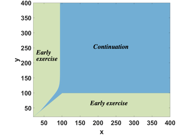
Figure 6.1: Early exercise regions for the American put-on-the-min at $t=T/2$, corresponding to Refine. level 4 from Table LABEL:tab:result01.

6.2.2 Put-on-the-average option

For the second test case, we examine an American option based on the arithmetic average of two assets. The payoff function, $\hat{v}(x,y)$, is defined as:

$$\hat{v}(x,y)=\max(K-(e^{x}+e^{y})/2,0),\quad K>0.$$ (6.2)

As a representative example, we use the modeling parameters from Case I, with initial asset values set at $X_{0}=100$ and $Y_{0}=100$ to illustrate the put-on-the-average option. The computed option prices, presented in Table LABEL:tab:result02, demonstrate a first order of convergence and show strong agreement with the results reported in [13]. In addition, the early exercise regions at $T/2$ for this case are depicted in Figure 6.2. Similar experiments conducted for Cases II and III yield comparable results. Further numerical results for American put-on-the-average options, encompassing various initial asset values and parameter sets, are presented in Section 6.2.5 [Table 6.10].

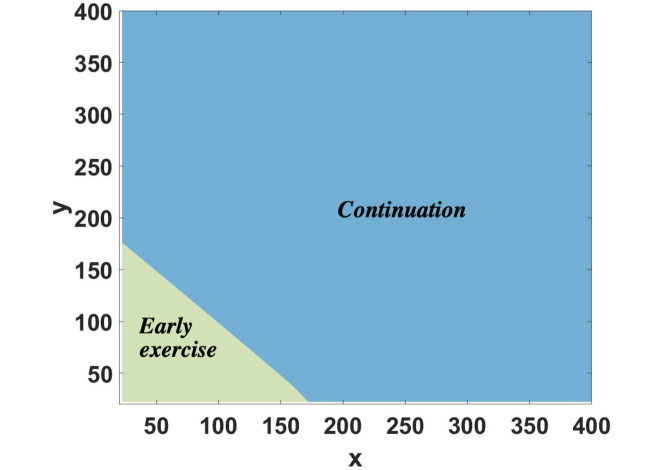
Figure 6.2: Early exercise regions for the American put-on-the-average at $t=T/2$, corresponding to Refine. level 4 from Table LABEL:tab:result02.

6.2.3 Impact of spatial domain sizes

In this subsection, we validate the adequacy of the chosen spatial domain for our experiments, focusing on Case I for brevity. Similar tests for Cases II and III yield consistent results and are omitted here.

To assess domain sufficiency, we revisit the setup from Table LABEL:tab:result01 and double the sizes of the interior sub-domain $\mathbb{D}_{\scalebox{0.7}{\text{in}}}$, extending $x_{\min}=\ln(X_{0})-1.5$, $x_{\max}=\ln(X_{0})+1.5$, $y_{\min}=\ln(Y_{0})-1.5$, and $y_{\max}=\ln(Y_{0})+1.5$ to $x_{\min}=\ln(X_{0})-3$, $x_{\max}=\ln(X_{0})+3$, $y_{\min}=\ln(Y_{0})-3$, and $y_{\max}=\ln(Y_{0})+3$. The boundary sub-domains are adjusted accordingly as in (4.9). We also double the intervals $N$ and $J$ to preserve $\Delta x$ and $\Delta y$ as in the setup from Table LABEL:tab:result01.

The computed option prices for this larger domain, presented in Table 6.6 under “Larger $\mathbb{D}_{\scalebox{0.7}{\text{in}}}$” show minimal differences from the original results (shown under “Table LABEL:tab:result01), with discrepancies only appearing at the 8th decimal place. These differences are recorded in the “Diff.” column, which represents the absolute difference between the computed option prices from Table LABEL:tab:result01 and those obtained with either an extended or contracted interior sub-domain $\mathbb{D}_{\scalebox{0.7}{\text{in}}}$. This indicates that further enlarging the spatial computational domain has a negligible effect on accuracy.

Refine.	Table LABEL:tab:result01	(Larger $\mathbb{D}_{\scalebox{0.7}{\text{in}}}$)		(Smaller $\mathbb{D}_{\scalebox{0.7}{\text{in}}}$)
level	Price	Price	Diff.	Price	Diff.
0	16.374702	16.374702	1.64e-08	16.374210	4.92e-04
1	16.383298	16.383298	1.60e-08	16.382820	4.78e-04
2	16.387210	16.387210	1.60e-08	16.386736	4.74e-04
3	16.389079	16.389079	1.62e-08	16.388605	4.74e-04
4	16.389991	16.389991	1.62e-08	16.389515	4.76e-04

Table 6.6: Prices (put-on-min) obtained using different spatial computational domain: (i) a Larger $\mathbb{D}_{\scalebox{0.7}{\text{in}}}$ with $x_{\min}=\ln(X_{0})-3$, $x_{\max}=\ln(X_{0})+3$, $y_{\min}=\ln(Y_{0})-3$, $y_{\max}=\ln(Y_{0})+3$, and (ii) a Smaller $\mathbb{D}_{\scalebox{0.7}{\text{in}}}$ with $x_{\min}=\ln(X_{0})-0.75$, $x_{\max}=\ln(X_{0})+0.75$, $y_{\min}=\ln(Y_{0})-0.75$, $y_{\max}=\ln(Y_{0})+0.75$. These are to compare with prices in Table LABEL:tab:result01 obtained using the original $\mathbb{D}_{\scalebox{0.7}{\text{in}}}$ with $z_{\min}=\ln(Z_{0})-1.5$, $z_{\max}=\ln(Z_{0})+1.5$, for $z\in\{x,y\}$ as in Table 6.3[Case 1].

In addition, we test a smaller interior domain $\mathbb{D}_{\scalebox{0.7}{\text{in}}}$ with boundaries $x_{\min}=\ln(X_{0})-0.75$, $x_{\max}=\ln(X_{0})+0.75$, $y_{\min}=\ln(Y_{0})-0.75$, and $y_{\max}=\ln(Y_{0})+0.75$, while keeping $\Delta x$ and $\Delta y$ constant. The results, shown in Table 6.6 under “Smaller $\mathbb{D}_{\scalebox{0.7}{\text{in}}}$”, reveal differences starting at the third decimal place compared to the original setup. This indicates that the selected domain size is essential for achieving accurate results; further expansion of the domain size offers negligible benefit, whereas any reduction may introduce noticeable errors.

In Table 6.7, we present the test results for extending and contracting $\mathbb{D}_{\scalebox{0.7}{\text{in}}}$ for the American put-on-average option, which yield similar conclusions to those observed previously.

Refine.	Table LABEL:tab:result02	(Larger $\mathbb{D}_{\scalebox{0.7}{\text{in}}}$)		(Smaller $\mathbb{D}_{\scalebox{0.7}{\text{in}}}$)
level	Price	Price	Diff.	Price	Diff.
0	3.431959	3.431959	2.91e-07	3.431348	6.12e-04
1	3.436727	3.436727	3.09e-07	3.436080	6.37e-04
2	3.439096	3.439096	3.21e-07	3.436080	6.69e-04
3	3.440278	3.440278	3.26e-07	3.438426	6.82e-04
4	3.440868	3.440868	3.29e-07	3.440178	6.91e-04

Table 6.7: Prices (put-on-average) obtained using different spatial computational domain: (i) a Larger $\mathbb{D}_{\scalebox{0.7}{\text{in}}}$ with $x_{\min}=\ln(X_{0})-3$, $x_{\max}=\ln(X_{0})+3$, $y_{\min}=\ln(Y_{0})-3$, $y_{\max}=\ln(Y_{0})+3$, and (ii) a Smaller $\mathbb{D}_{\scalebox{0.7}{\text{in}}}$ with $x_{\min}=\ln(X_{0})-0.75$, $x_{\max}=\ln(X_{0})+0.75$, $y_{\min}=\ln(Y_{0})-0.75$, $y_{\max}=\ln(Y_{0})+0.75$. These are to compare with prices in Table LABEL:tab:result02 obtained using the original $\mathbb{D}_{\scalebox{0.7}{\text{in}}}$ with $z_{\min}=\ln(Z_{0})-1.5$, $z_{\max}=\ln(Z_{0})+1.5$, for $z\in\{x,y\}$, as in Table 6.3[Case 1].

6.2.4 Impact of boundary conditions

In this subsection, we numerically demonstrate that our straightforward approach of employing discounted payoffs for boundary sub-domains is adequate. For brevity, we show the tests of impact of boundary conditions for Case I. Similar experiments for Cases II and III yield the same results.

We revisited previous experiments reported in Tables LABEL:tab:result01, introducing more sophisticated boundary conditions based on the asymptotic behavior of the PIDEs (3.1) as $z\to-\infty$ and $z\to\infty$ for $z\in\{x,y\}$ as proposed in [19]. Specifically, the PIDEs (3.1) simplifies to the 1D PDEs shown in (6.3) when $x$ or $y$ tends to $-\infty$:

$$v_{\tau}-\big{(}r-(\sigma_{y})^{2}/2\big{)}v_{y}+(\sigma_{y})^{2}/2v_{yy}+rv =0,\quad x\to-\infty,$$ (6.3)

$$v_{\tau}-\big{(}r-(\sigma_{x})^{2}/2\big{)}v_{x}+(\sigma_{x})^{2}/2v_{xx}+rv =0,\quad y\to-\infty.$$

That can be justified based on the properties of the Green’s function of the PIDE [36]. As $x,y\to-\infty$, the PIDEs (3.1) simplifies to the ordinary differential equation $v_{\tau}+rv=0$.

To adhere to these asymptotic boundary conditions, we choose a much large spatial domain: $x_{\min}=\ln(X_{0})-12$, $x_{\max}=\ln(X_{0})+12$, $y_{\min}=\ln(Y_{0})-12$, $y_{\max}=\ln(Y_{0})+12$, and adjust the number of intervals $N$ and $J$ accordingly to maintain the same grid resolution ($\Delta x$ and $\Delta y$). Employing the monotone integration technique, tailored for the 1D case, we effectively solved the 1D PDEs in (6.3). The ordinary differential equation $v_{\tau}+rv=0$ is solved directly and efficiently. The scheme’s convergence to the viscosity solution can be rigorously established in the same fashion as the propose scheme.

	Put-on-the-min		Put-on-the-average
Refine.	Price	Price	Price	Price
level		(Table LABEL:tab:result01)		(Table LABEL:tab:result02)
0	16.374702	16.374702	3.431959	3.431959
1	16.383298	16.383298	3.436727	3.436727
2	16.387210	16.387210	3.439096	3.439096
3	16.389079	16.389079	3.440278	3.440278
4	16.389991	16.389991	3.440868	3.440868

Table 6.8: Results using sophisticated boundary conditions. Compare with computed prices in Table LABEL:tab:result01 and Table LABEL:tab:result02 where discounted payoff boundary conditions are used.

The computed option prices for the put-on-the-min option, as shown in Table 6.8, are virtually identical with those from the original setup (see column marked “Table. LABEL:tab:result01”). In addition, Table 6.8 presents results for the put-on-the-average option using the similar sophisticated boundary condition, with findings consistent with the put-on-the-min option. These results confirm that our simple boundary conditions are not only easy to implement but also sufficient to meet the theoretical and practical requirements of our numerical experiments.

6.2.5 Comprehensive tests

In the following, we present a detailed study of two types of options: an American put-on-the-min option and an American put-on-the-average option, tested with various strike prices $K$ and initial asset values. Across all three parameter cases, our computed prices closely align with the reference prices given in [13][Tables 5 and 6]. However, slight discrepancies appear in some cases, likely due to the finer grid resolution used in this paper, which may contribute to increased precision in our results. Put-on-average Case I $Y_{0}$ $X_{0}$ 90 100 110 MI 90 10.000000 5.987037 3.440343 100 6.028929 3.440868 1.886527 110 3.490665 1.890874 0.992933 Ref. [13] $90$ 10.003 5.989 3.441 $100$ 6.030 3.442 1.877 $110$ 3.491 1.891 0.993 Case II 36 40 44 MI 36 5.405825 4.363340 3.547399 40 4.213899 3.338840 2.669076 44 3.224979 2.506688 1.969401 Ref. [13] $36$ 5.406 4.363 3.547 $40$ 4.214 3.339 2.669 $44$ 3.225 2.507 1.969 Case III 36 40 44 MI 36 12.472058 11.935904 11.446078 40 11.439979 10.948971 10.500581 44 10.499147 10.049777 9.639534 Ref. [13] $36$ 12.466 11.930 11.440 $40$ 11.434 10.943 10.495 $44$ 10.493 10.043 9.633 Table 6.10: Results for an American put-on-average option under Cases I, II, III. Reference prices by FD method (operator splitting) from [13][Table 6].

7 Conclusion and future work

In this paper, we address a critical gap in the numerical analysis of two-asset American options under the Merton jump-diffusion model by introducing an efficient and straightforward-to-implement monotone scheme based on numerical integration. The pricing of these options involves solving complex 2-D variational inequalities that include cross derivative and nonlocal integro-differential terms due to jumps. Traditional finite difference methods often struggle to maintain monotonicity in cross derivative approximations—crucial for ensuring convergence to the viscosity solution-and accurately discretize 2-D jump integrals. Our approach overcomes these challenges by leveraging an infinite series representation of the Green’s function, where each term is non-negative and computable, enabling efficient approximation of 2-D convolution integrals through a monotone integration method. In addition, we rigorously establish the stability and consistency of the proposed scheme in the viscosity sense and prove its convergence to the viscosity solution of the variational inequality. This overcomes several significant limitations associated with previous numerical techniques.

Extensive numerical results demonstrate strong agreement with benchmark solutions from published test cases, including those obtained via operator splitting methods, highlighting the utility of our approach as a valuable reference for verifying other numerical techniques.

Although our focus has been on the two-asset Merton jump-diffusion model, the methods developed here—particularly the infinite series representation of the Green’s function—have broader applicability. While we utilize the closed-form Fourier transform of the Green’s function in this model, iterative techniques for differential-integral operators, such as those discussed in [35], could be used to extend this framework to other, more general jump-diffusion models. Exploring such extensions and applying this framework to a wider range of financial models remains an exciting direction for future research.

Appendices

Appendix A Proof of Lemma 2.1

We extend the methods from [22], originally developed for 1-D European options, to address 2-D variational inequalities (2.4) and (2.9). For simplicity, we denote by $d(\tau)$ the discounting factor. The solution $v^{\prime}({\bf{x}})$ to the full-domain variational inequality (2.4) is simply

$$v^{\prime}({\bf{x}})=\sup_{\gamma\in[0,\tau]}\mathbb{E}_{\tau}^{\scalebox{0.6}{$x$},\scalebox{0.6}{$y$}}\left[d(\tau)\hat{v}({\color[rgb]{0,0,0}^{{}^{\prime}}_{\gamma}},{\color[rgb]{0,0,0}^{{}^{\prime}}_{\gamma}})\right],$$

which comes from (2.3) with a change of variables from $\left(X_{t},Y_{t}\right)$ to $(X^{\prime}_{t},Y^{\prime}_{t})=\left(\ln(X_{t}),\ln(Y_{t})\right)$ and from $t$ to $\tau$. To obtain a probabilistic representation of the solution $v({\bf{x}})$ to the localized variational inequality (2.9), for fixed ${\bf{x}}=(x,y,\tau)$, we define the random variables $M_{\tau}^{x}=\sup_{\varsigma\in[0,\tau]}|{\color[rgb]{0,0,0}^{{}^{\prime}}_{\varsigma}}+x|$ and $M_{\tau}^{y}=\sup_{\varsigma\in[0,\tau]}|{\color[rgb]{0,0,0}^{{}^{\prime}}_{\varsigma}}+y|$ to respectively represent the maximum deviation of processes $\{{\color[rgb]{0,0,0}^{{}^{\prime}}_{\varsigma}}\}$ and $\{{\color[rgb]{0,0,0}^{{}^{\prime}}_{\varsigma}}\}$ from $x$ and $y$ over the interval $[0,\tau]$. We also define the random variable $\theta(x)=\inf\{\varsigma\geq 0,|{\color[rgb]{0,0,0}^{{}^{\prime}}_{\varsigma}}+x|\geq A\}$ as the first exit time of the process $\{{\color[rgb]{0,0,0}^{{}^{\prime}}_{\varsigma}}+x\}$ from $[-A,A]$. Similarly, the random variable $\theta(y)$ is defined for the process $\{{\color[rgb]{0,0,0}^{{}^{\prime}}_{\varsigma}}+y\}$. Using these random variables, $v({\bf{x}})$ can be expressed as

$$v({\bf{x}})=\sup_{\gamma\in[0,\tau]}\mathbb{E}_{\tau}^{\scalebox{0.6}{$x$},\scalebox{0.6}{$y$}}\left[d(\tau)\left(\hat{v}({\color[rgb]{0,0,0}^{{}^{\prime}}_{\gamma}},{\color[rgb]{0,0,0}^{{}^{\prime}}_{\gamma}})\mathbb{I}_{\left\{\{M_{\tau}^{x}<A\}\cap\{M_{\tau}^{y}<A\}\right\}}+\hat{p}({\color[rgb]{0,0,0}^{{}^{\prime}}_{\gamma}},{\color[rgb]{0,0,0}^{{}^{\prime}}_{\theta(y)}})\mathbb{I}_{\left\{\{M_{\tau}^{x}<A\}\cap\{M_{\tau}^{y}\geq A\}\right\}}\right.\right.$$

$$\qquad\qquad\left.\left.+\hat{p}({\color[rgb]{0,0,0}^{{}^{\prime}}_{\theta(x)}},{\color[rgb]{0,0,0}^{{}^{\prime}}_{\gamma}})\mathbb{I}_{\left\{\{M_{\tau}^{x}\geq A\}\cap\{M_{\tau}^{y}<A\}\right\}}+\hat{p}({\color[rgb]{0,0,0}^{{}^{\prime}}_{\theta(x)}},{\color[rgb]{0,0,0}^{{}^{\prime}}_{\theta(y)}})\mathbb{I}_{\left\{\{M_{\tau}^{x}\geq A\}\cap\{M_{\tau}^{y}\geq A\}\right\}}\right)\right].$$

Subtracting $v(\cdot)$ from $v^{\prime}(\cdot)$ gives $\left|v^{\prime}({\bf{x}})-v({\bf{x}})\right|\leq\ldots$

$$\ldots \leq\sup_{\gamma\in[0,\tau]}\left|\mathbb{E}_{\tau}^{\scalebox{0.6}{$x$},\scalebox{0.6}{$y$}}\left[d(\tau)\left(\hat{v}({\color[rgb]{0,0,0}^{{}^{\prime}}_{\gamma}},{\color[rgb]{0,0,0}^{{}^{\prime}}_{\gamma}})\mathbb{I}_{\left\{\{M_{\tau}^{x}\geq A\}\cup\{M_{\tau}^{y}\geq A\}\right\}}-\hat{p}({\color[rgb]{0,0,0}^{{}^{\prime}}_{\gamma}},{\color[rgb]{0,0,0}^{{}^{\prime}}_{\theta(y)}})\mathbb{I}_{\left\{\{M_{\tau}^{x}<A\}\cap\{M_{\tau}^{y}\geq A\}\right\}}\right.\right.\right.$$

$$\qquad\qquad\left.\left.\left.-\hat{p}({\color[rgb]{0,0,0}^{{}^{\prime}}_{\theta(x)}},{\color[rgb]{0,0,0}^{{}^{\prime}}_{\gamma}})\mathbb{I}_{\left\{\{M_{\tau}^{x}\geq A\}\cap\{M_{\tau}^{y}<A\}\right\}}-\hat{p}({\color[rgb]{0,0,0}^{{}^{\prime}}_{\theta(x)}},{\color[rgb]{0,0,0}^{{}^{\prime}}_{\theta(y)}})\mathbb{I}_{\left\{\{M_{\tau}^{x}\geq A\}\cap\{M_{\tau}^{y}\geq A\}\right\}}\right)\right]\right|,$$

$$\leq \sup_{\gamma\in[0,\tau]}d(\tau)\left[\mathbb{E}_{\tau}^{\scalebox{0.6}{$x$},\scalebox{0.6}{$y$}}\left|\hat{v}({\color[rgb]{0,0,0}^{{}^{\prime}}_{\gamma}},{\color[rgb]{0,0,0}^{{}^{\prime}}_{\gamma}})\mathbb{I}_{\left\{\{M_{\tau}^{x}\geq A\}\cup\{M_{\tau}^{y}\geq A\}\right\}}\right|+\mathbb{E}_{\tau}^{\scalebox{0.6}{$x$},\scalebox{0.6}{$y$}}\left|\hat{p}({\color[rgb]{0,0,0}^{{}^{\prime}}_{\gamma}},{\color[rgb]{0,0,0}^{{}^{\prime}}_{\theta(y)}})\mathbb{I}_{\left\{\{M_{\tau}^{x}<A\}\cap\{M_{\tau}^{y}\geq A\}\right\}}\right|\right.$$

$$\qquad\qquad\left.+\mathbb{E}_{\tau}^{\scalebox{0.6}{$x$},\scalebox{0.6}{$y$}}\left|\hat{p}({\color[rgb]{0,0,0}^{{}^{\prime}}_{\theta(x)}},{\color[rgb]{0,0,0}^{{}^{\prime}}_{\gamma}})\mathbb{I}_{\left\{\{M_{\tau}^{x}\geq A\}\cap\{M_{\tau}^{y}<A\}\right\}}\right|+\mathbb{E}_{\tau}^{\scalebox{0.6}{$x$},\scalebox{0.6}{$y$}}\left|\hat{p}({\color[rgb]{0,0,0}^{{}^{\prime}}_{\theta(x)}},{\color[rgb]{0,0,0}^{{}^{\prime}}_{\theta(y)}})\mathbb{I}_{\left\{\{M_{\tau}^{x}\geq A\}\cap\{M_{\tau}^{y}\geq A\}\right\}}\right|\right],$$

$$\leq \sup_{\gamma\in[0,\tau]}d(\tau)\left[\left\|\hat{v}\right\|_{\infty}\mathfrak{Q}\left(\{M_{\tau}^{x}\geq A\}\cup\{M_{\tau}^{y}\geq A\}\right)+\left\|\hat{p}\right\|_{\infty}\mathfrak{Q}\left(\{M_{\tau}^{x}\geq A\}\cup\{M_{\tau}^{y}\geq A\}\right)\right],$$

$$\leq \sup_{\gamma\in[0,\tau]}d(\tau)\left[\left(\left\|\hat{v}\right\|_{\infty}+\left\|\hat{p}\right\|_{\infty}\right)\left(\mathfrak{Q}\left(M_{\tau}^{x}\geq A\right)+\mathfrak{Q}\left(M_{\tau}^{y}\geq A\right)\right)\right],$$

$$\leq \sup_{\gamma\in[0,\tau]}d(\tau)\left[\left(\left\|\hat{v}\right\|_{\infty}+\left\|\hat{p}\right\|_{\infty}\right)\left(\mathfrak{Q}\left(M_{\tau}^{0}\geq A-|x|\right)+\mathfrak{Q}\left(M_{\tau}^{0}\geq A-|y|\right)\right)\right],$$

$${\buildrel(\text{i})\over{\leq}} \sup_{\gamma\in[0,\tau]}d(\tau)\left[\left(\left\|\hat{v}\right\|_{\infty}+\left\|\hat{p}\right\|_{\infty}\right)C^{\prime}(\tau)\left({\color[rgb]{0,0,0}{e^{-(A-|x|)}+e^{-(A-|y|)}}}\right)\right],$$

$$= ~{}C(\tau)\left(\left\|\hat{v}\right\|_{\infty}+\left\|\hat{p}\right\|_{\infty}\right)\left(e^{-(A-|x|)}+e^{-(A-|y|)}\right).$$

Here, (i) is due to Theorem 25.18 of [43] and Markov’s inequality; $C(\tau)$ is a positive bounded constant that does not depend on $x_{\scalebox{0.55}{$\min$}}$, $x_{\scalebox{0.55}{$\max$}}$, $y_{\scalebox{0.55}{$\min$}}$, and $y_{\scalebox{0.55}{$\max$}}$. This concludes the proof.

Appendix B Proof of Lemma 3.1

By the inverse Fourier transform $\mathfrak{F}^{-1}[\cdot]$ in (3.2) and the closed-form expression for $G({\boldsymbol{\eta}},\Delta\tau)$ in (3.5), we have

$$g({\boldsymbol{z}},\Delta\tau)~{}=~{} \frac{1}{(2\pi)^{2}}\,\int_{\mathbb{R}^{2}}e^{i{\boldsymbol{\eta}}\cdot{\boldsymbol{z}}}e^{\Psi({\boldsymbol{\eta}})\Delta\tau}~{}d{\boldsymbol{\eta}}~{}=~{}\frac{1}{(2\pi)^{2}}\,\int_{\mathbb{R}^{2}}e^{-\frac{1}{2}{\boldsymbol{\eta}}^{\top}\boldsymbol{C}{\boldsymbol{\eta}}+i\left({\boldsymbol{\beta}}+{\boldsymbol{z}}\right)\cdot{\boldsymbol{\eta}}+\theta}\,e^{\lambda\Gamma\left({\boldsymbol{\eta}}\right)\Delta\tau}~{}d{\boldsymbol{\eta}},$$

where $$\boldsymbol{C}=\Delta\tau\,\tilde{\boldsymbol{C}},\quad{\boldsymbol{\beta}}=\Delta\tau\,\tilde{{\boldsymbol{\beta}}},\quad\theta=-(r+\lambda)\Delta\tau.$$ (B.1)

Following the approach developed in [27, 65, 12], we expand the term $e^{\lambda\Gamma({\boldsymbol{\eta}})\Delta\tau}$ in (B) in a Taylor series, noting that

$$\left(\Gamma({\boldsymbol{\eta}})\right)^{k} =\left(\int_{\mathbb{R}^{2}}f({\boldsymbol{s}})\exp(i{\boldsymbol{\eta}}\cdot{\boldsymbol{s}})d{\boldsymbol{s}}\right)^{k}$$

$$=\left(\int_{\mathbb{R}^{2}}f({\boldsymbol{s}}_{1})\exp(i{\boldsymbol{\eta}}\cdot{\boldsymbol{s}}_{1})d{\boldsymbol{s}}_{1}\right)\left(\int_{\mathbb{R}^{2}}f({\boldsymbol{s}}_{2})\exp(i{\boldsymbol{\eta}}\cdot{\boldsymbol{s}}_{2})d{\boldsymbol{s}}_{2}\right)\ldots\left(\int_{\mathbb{R}^{2}}f({\boldsymbol{s}}_{k})\exp(i{\boldsymbol{\eta}}\cdot{\boldsymbol{s}}_{k})d{\boldsymbol{s}}_{k}\right)$$

$$=\int_{\mathbb{R}^{2}}\ldots\int_{\mathbb{R}^{2}}f({\boldsymbol{s}}_{1})f({\boldsymbol{s}}_{2})\ldots f({\boldsymbol{s}}_{k})\exp\left(i{\boldsymbol{\eta}}\cdot{\boldsymbol{s}}_{1}\right)\exp\left(i{\boldsymbol{\eta}}\cdot{\boldsymbol{s}}_{2}\right)\ldots\exp\left(i{\boldsymbol{\eta}}\cdot{\boldsymbol{s}}_{k}\right)d{\boldsymbol{s}}_{1}d{\boldsymbol{s}}_{2}\ldots d{\boldsymbol{s}}_{k},$$

$$=\int_{\mathbb{R}^{2}}\ldots\int_{\mathbb{R}^{2}}\prod_{\ell=1}^{k}f({\boldsymbol{s}}_{\ell})\exp\left(i{\boldsymbol{\eta}}\cdot{\boldsymbol{S}}_{k}\right)d{\boldsymbol{s}}_{1}d{\boldsymbol{s}}_{2}\ldots d{\boldsymbol{s}}_{k}.$$ (B.2)

Here, ${\boldsymbol{s}}_{\ell}=[s_{1},s_{2}]_{\ell}$ is the $\ell$-th column vector, and each pair of ${\boldsymbol{s}}_{i}$ and ${\boldsymbol{s}}_{j}$ being independent and identically distributed (i.i.d) for $i\neq j$, ${{\boldsymbol{S}}}_{k}=\sum_{\ell=1}^{k}{\boldsymbol{s}}_{\ell}=\sum_{\ell=1}^{k}[s_{1},s_{2}]_{\ell}$, with ${{\boldsymbol{S}}}_{0}=[0,0]$, and for $k=0$, $\left(\Gamma({\boldsymbol{\eta}})\right)^{0}=1$. Then, we have the Taylor series for $e^{\lambda\Gamma({\boldsymbol{\eta}})\Delta\tau}$ as follows

$$e^{\lambda\Gamma({\boldsymbol{\eta}})\Delta\tau}=\sum_{k=0}^{\infty}\frac{\left(\lambda\Delta\tau\right)^{k}}{k!}(\Gamma({\boldsymbol{\eta}}))^{k}=\sum_{k=0}^{\infty}\frac{\left(\lambda\Delta\tau\right)^{k}}{k!}\int_{\mathbb{R}^{2}}\ldots\int_{\mathbb{R}^{2}}\prod_{\ell=1}^{k}f({\boldsymbol{s}}_{\ell})\exp\left(i{\boldsymbol{\eta}}\cdot{\boldsymbol{S}}_{k}\right)d{\boldsymbol{s}}_{1}d{\boldsymbol{s}}_{2}\ldots d{\boldsymbol{s}}_{k}.$$ (B.3)

We now substitute equation (B.3) into the Green’s function $g({\boldsymbol{z}},\Delta\tau)$ in (B), which is expressed through substitutions as

$$g({\boldsymbol{z}},\Delta\tau)=\frac{1}{(2\pi)^{2}}\sum_{k=0}^{\infty}\frac{\left(\lambda\Delta\tau\right)^{k}}{k!}\int_{\mathbb{R}^{2}}e^{-\frac{1}{2}{\boldsymbol{\eta}}^{\top}\mathbf{C}{\boldsymbol{\eta}}+i\left({\boldsymbol{\beta}}+{\boldsymbol{z}}\right)\cdot{\boldsymbol{\eta}}+\theta}\,\int_{\mathbb{R}^{2}}\ldots\int_{\mathbb{R}^{2}}\prod_{\ell=1}^{k}f({\boldsymbol{s}}_{\ell})\exp\left(i{\boldsymbol{\eta}}\cdot{\boldsymbol{S}}_{k}\right)d{\boldsymbol{s}}_{1}d{\boldsymbol{s}}_{2}\ldots d{\boldsymbol{s}}_{k}~{}d{\boldsymbol{\eta}}$$

$${\buildrel(\text{i})\over{=}}~{}\frac{1}{(2\pi)^{2}}\sum_{k=0}^{\infty}\frac{\left(\lambda\Delta\tau\right)^{k}}{k!}\,\int_{\mathbb{R}^{2}}\ldots\int_{\mathbb{R}^{2}}\prod_{\ell=1}^{k}f({\boldsymbol{s}}_{\ell})\int_{\mathbb{R}^{2}}e^{-\frac{1}{2}{\boldsymbol{\eta}}^{\top}\mathbf{C}{\boldsymbol{\eta}}+i\left({\boldsymbol{\beta}}+{\boldsymbol{z}}+{\boldsymbol{S}}_{k}\right)\cdot{\boldsymbol{\eta}}+\theta}~{}d{\boldsymbol{\eta}}\,d{\boldsymbol{s}}_{1}d{\boldsymbol{s}}_{2}\ldots d{\boldsymbol{s}}_{k}{\buildrel(\text{ii})\over{=}}\ldots$$

$$\frac{1}{2\pi\sqrt{\det(\boldsymbol{C})}}\sum_{k=0}^{\infty}\frac{\left(\lambda\Delta\tau\right)^{k}}{k!}\int_{\mathbb{R}^{2}}\ldots\int_{\mathbb{R}^{2}}\exp\left(\theta-\frac{\left({\boldsymbol{\beta}}+{\boldsymbol{z}}+{\boldsymbol{S}}_{k}\right)^{\top}\boldsymbol{C}^{-1}({\boldsymbol{\beta}}+{\boldsymbol{z}}+{\boldsymbol{S}}_{k})}{2}\right)\left(\prod_{\ell=1}^{k}f({\boldsymbol{s}}_{\ell})\right)d{\boldsymbol{s}}_{1}\ldots d{\boldsymbol{s}}_{k}.$$

Here, (i) is due to the Fubini’s theorem, in (ii), we apply the result for the multidimensional Gaussian-type integral, i.e $\int_{\mathbb{R}^{n}}\exp(-\frac{1}{2}{\bf{x}}^{\top}\boldsymbol{A}{\bf{x}}+\boldsymbol{b}^{\top}{\bf{x}}+c)~{}d{\bf{x}}=\sqrt{\det(2\pi\boldsymbol{A}^{-1})}e^{\frac{1}{2}\boldsymbol{b}^{\top}\boldsymbol{A}^{-1}\boldsymbol{b}+c}$, and the determinant, $\det(\boldsymbol{C})=\det(\Delta\tau\,\tilde{\boldsymbol{C}})=(\Delta\tau)^{2}\det(\tilde{\boldsymbol{C}})=(\Delta\tau)^{2}\sigma_{\scalebox{0.6}{$x$}}^{2}\sigma_{\scalebox{0.6}{$y$}}^{2}(1-\rho^{2})$.

Appendix C Proof of Corollary 3.1

Recalling (3.6), we have $g({\boldsymbol{z}};\Delta t)=\frac{\exp\left(\theta-\frac{\left({\boldsymbol{\beta}}+{\boldsymbol{z}}\right)^{\top}\boldsymbol{C}^{-1}({\boldsymbol{\beta}}+{\boldsymbol{z}})}{2}\right)}{2\pi\sqrt{\det(\boldsymbol{C})}}\ldots$

$$\ldots +\frac{e^{\theta}}{2\pi\sqrt{\det(\boldsymbol{C})}}\sum_{k=1}^{\infty}\frac{\left(\lambda\Delta\tau\right)^{k}}{k!}\underbrace{\int_{\mathbb{R}^{2}}\ldots\int_{\mathbb{R}^{2}}\exp\left(-\frac{\left({\boldsymbol{\beta}}+{\boldsymbol{z}}+{\boldsymbol{S}}_{k}\right)^{\top}\boldsymbol{C}^{-1}({\boldsymbol{\beta}}+{\boldsymbol{z}}+{\boldsymbol{S}}_{k})}{2}\right)\left(\prod_{\ell=1}^{k}f({\boldsymbol{s}}_{\ell})\right)d{\boldsymbol{s}}_{1}\ldots d{\boldsymbol{s}}_{k}}_{E_{k}}$$

$$=\frac{\exp\left(\theta-\frac{\left({\boldsymbol{\beta}}+{\boldsymbol{z}}\right)^{\top}\boldsymbol{C}^{-1}({\boldsymbol{\beta}}+{\boldsymbol{z}})}{2}\right)}{2\pi\sqrt{\det(\boldsymbol{C})}}+\frac{e^{\theta}}{2\pi\sqrt{\det(\boldsymbol{C})}}\sum_{k=1}^{\infty}\frac{\left(\lambda\Delta\tau\right)^{k}}{k!}~{}E_{k}.$$ (C.1)

Here, the term $E_{k}$ in (C) is clearly non-negative and can be computed as

$$E_{k}=\int_{\mathbb{R}^{2}}\exp\left(-\frac{\left({\boldsymbol{\beta}}+{\boldsymbol{z}}+{\boldsymbol{s}}\right)^{\top}\boldsymbol{C}^{-1}({\boldsymbol{\beta}}+{\boldsymbol{z}}+{\boldsymbol{s}})}{2}\right)f_{\hat{{\boldsymbol{\xi}}}_{k}}({\boldsymbol{s}})~{}d{\boldsymbol{s}},$$ (C.2)

where $f_{\hat{{\boldsymbol{\xi}}}_{k}}({\boldsymbol{s}})$ is the PDF of the random variable $\hat{{\boldsymbol{\xi}}}_{k}=\sum_{\ell=1}^{k}\ln({\boldsymbol{\xi}})_{\ell}=\sum_{\ell=1}^{k}[\ln(\xi_{\scalebox{0.6}{$x$}}),\ln(\xi_{\scalebox{0.6}{$y$}})]_{\ell}$ which is the sum of i.i.d random variables for fixed $k$. For the Merton case, we have $\hat{{\boldsymbol{\xi}}}_{k}\sim\text{Normal}\left(k{\boldsymbol{\widetilde{\mu}}},k\boldsymbol{C}_{M}\right)$ with the PDF

$$f_{\hat{{\boldsymbol{\xi}}}_{k}}({\boldsymbol{s}})=\frac{\exp\left(-\frac{\left({\boldsymbol{s}}-k{\boldsymbol{\widetilde{\mu}}}\right)^{\top}(k\boldsymbol{C}_{M})^{-1}({\boldsymbol{s}}-k{\boldsymbol{\widetilde{\mu}}})}{2}\right)}{2\pi\sqrt{\det(k\boldsymbol{C}_{M})}}.$$ (C.3)

By substituting the equation (C.3) into (C.2), we have

$$E_{k} =\int_{\mathbb{R}^{2}}\exp\left(-\frac{\left({\boldsymbol{\beta}}+{\boldsymbol{z}}+{\boldsymbol{s}}\right)^{\top}\boldsymbol{C}^{-1}({\boldsymbol{\beta}}+{\boldsymbol{z}}+{\boldsymbol{s}})}{2}\right)\frac{\exp\left(-\frac{\left({\boldsymbol{s}}-k{\boldsymbol{\widetilde{\mu}}}\right)^{\top}(k\boldsymbol{C}_{M})^{-1}({\boldsymbol{s}}-k{\boldsymbol{\widetilde{\mu}}})}{2}\right)}{2\pi\sqrt{\det(k\boldsymbol{C}_{M})}}~{}d{\boldsymbol{s}}$$

$$=\frac{1}{2\pi\sqrt{\det(k\boldsymbol{C}_{M})}}\int_{\mathbb{R}^{2}}\exp\left(-\frac{\left({\boldsymbol{\beta}}+{\boldsymbol{z}}+{\boldsymbol{s}}\right)^{\top}\boldsymbol{C}^{-1}({\boldsymbol{\beta}}+{\boldsymbol{z}}+{\boldsymbol{s}})+\left({\boldsymbol{s}}-k{\boldsymbol{\widetilde{\mu}}}\right)^{\top}(k\boldsymbol{C}_{M})^{-1}({\boldsymbol{s}}-k{\boldsymbol{\widetilde{\mu}}})}{2}\right)~{}d{\boldsymbol{s}}$$

$${\buildrel(\text{i})\over{=}}\frac{1}{2\pi\sqrt{\det(k\boldsymbol{C}_{M})}}\int_{\mathbb{R}^{2}}\exp\left(-\frac{{\boldsymbol{s}}^{\top}\left(\boldsymbol{C}^{-1}+(k\boldsymbol{C}_{M})^{-1}\right){\boldsymbol{s}}}{2}+\left((k{\boldsymbol{\widetilde{\mu}}})^{\top}(k\boldsymbol{C}_{M})^{-1}-({\boldsymbol{\beta}}+{\boldsymbol{z}})^{\top}\boldsymbol{C}^{-1}\right){\boldsymbol{s}}\ldots\right.$$

$$\qquad\left.\ldots-\frac{({\boldsymbol{\beta}}+{\boldsymbol{z}})^{\top}\boldsymbol{C}^{-1}({\boldsymbol{\beta}}+{\boldsymbol{z}})+(k{\boldsymbol{\widetilde{\mu}}})^{\top}(k\boldsymbol{C}_{M})^{-1}(k{\boldsymbol{\widetilde{\mu}}})}{2}\right)~{}d{\boldsymbol{s}}$$ (C.4)

Here, in (i), we use matrix multiplication distributive and associative properties. For simplicity, we adopt the following notational convention: $\boldsymbol{A}=\boldsymbol{C}^{-1}+(k\boldsymbol{C}_{M})^{-1}$, which is positive semi-definite and symmetric, and $\boldsymbol{\alpha}={\boldsymbol{\beta}}+{\boldsymbol{z}}$. Then, equation (C) becomes

$$E_{k} =\frac{1}{2\pi\sqrt{\det(k\boldsymbol{C}_{M})}}\int_{\mathbb{R}^{2}}\exp\left(-\frac{{\boldsymbol{s}}^{\top}\boldsymbol{A}{\boldsymbol{s}}}{2}+\left((k{\boldsymbol{\widetilde{\mu}}})^{\top}(k\boldsymbol{C}_{M})^{-1}-\boldsymbol{\alpha}^{\top}\boldsymbol{C}^{-1}\right){\boldsymbol{s}}\ldots\right.$$

$$\qquad\left.\ldots-\frac{\boldsymbol{\alpha}^{\top}\boldsymbol{C}^{-1}\boldsymbol{\alpha}+(k{\boldsymbol{\widetilde{\mu}}})^{\top}(k\boldsymbol{C}_{M})^{-1}(k{\boldsymbol{\widetilde{\mu}}})}{2}\right)~{}d{\boldsymbol{s}}$$

$${\buildrel(\text{i})\over{=}}\frac{\sqrt{\det\left(\boldsymbol{A}^{-1}\right)}}{\sqrt{\det(k\boldsymbol{C}_{M})}}\exp\left(\frac{\left((k{\boldsymbol{\widetilde{\mu}}})^{\top}(k\boldsymbol{C}_{M})^{-1}-\boldsymbol{\alpha}^{\top}\boldsymbol{C}^{-1}\right)\boldsymbol{A}^{-1}\left((k{\boldsymbol{\widetilde{\mu}}})^{\top}(k\boldsymbol{C}_{M})^{-1}-\boldsymbol{\alpha}^{\top}\boldsymbol{C}^{-1}\right)^{\top}}{2}\ldots\right.$$

$$\qquad\left.\ldots-\frac{\boldsymbol{\alpha}^{\top}\boldsymbol{C}^{-1}\boldsymbol{\alpha}+(k{\boldsymbol{\widetilde{\mu}}})^{\top}(k\boldsymbol{C}_{M})^{-1}(k{\boldsymbol{\widetilde{\mu}}})}{2}\right)$$

$$=\frac{\sqrt{\det\left(\boldsymbol{A}^{-1}\right)}}{\sqrt{\det(k\boldsymbol{C}_{M})}}\exp\left(\frac{\left((k{\boldsymbol{\widetilde{\mu}}})^{\top}(\boldsymbol{A}-\boldsymbol{C}^{-1})-\boldsymbol{\alpha}^{\top}\left(\boldsymbol{A}-(k\boldsymbol{C}_{M})^{-1}\right)\right)\boldsymbol{A}^{-1}\left((k{\boldsymbol{\widetilde{\mu}}})^{\top}(k\boldsymbol{C}_{M})^{-1}-\boldsymbol{\alpha}^{\top}\boldsymbol{C}^{-1}\right)^{\top}}{2}\ldots\right.$$

$$\qquad\left.\ldots-\frac{\boldsymbol{\alpha}^{\top}\boldsymbol{C}^{-1}\boldsymbol{\alpha}+(k{\boldsymbol{\widetilde{\mu}}})^{\top}(k\boldsymbol{C}_{M})^{-1}(k{\boldsymbol{\widetilde{\mu}}})}{2}\right)$$

$${\buildrel(\text{ii})\over{=}}\frac{\sqrt{\det\left(\boldsymbol{A}^{-1}\right)}}{\sqrt{\det(k\boldsymbol{C}_{M})}}\exp\left(\frac{1}{2}\left((k{\boldsymbol{\widetilde{\mu}}})^{\top}\boldsymbol{A}\boldsymbol{A}^{-1}(k\boldsymbol{C}_{M})^{-1}(k{\boldsymbol{\widetilde{\mu}}})-(k{\boldsymbol{\widetilde{\mu}}})^{\top}\boldsymbol{C}^{-1}\boldsymbol{A}^{-1}(k\boldsymbol{C}_{M})^{-1}(k{\boldsymbol{\widetilde{\mu}}})\ldots\right.\right.$$

$$\qquad\left.\left.\ldots+\boldsymbol{\alpha}^{\top}\boldsymbol{A}\boldsymbol{A}^{-1}\boldsymbol{C}^{-1}\boldsymbol{\alpha}-\boldsymbol{\alpha}^{\top}(k\boldsymbol{C}_{M})^{-1}\boldsymbol{A}^{-1}\boldsymbol{C}^{-1}\boldsymbol{\alpha}\right)-\frac{\boldsymbol{\alpha}^{\top}\boldsymbol{C}^{-1}\boldsymbol{\alpha}+(k{\boldsymbol{\widetilde{\mu}}})^{\top}(k\boldsymbol{C}_{M})^{-1}(k{\boldsymbol{\widetilde{\mu}}})}{2}\right)$$

$${\buildrel(\text{iii})\over{=}}\frac{\sqrt{\det\left(\boldsymbol{C}(\boldsymbol{C}+k\boldsymbol{C}_{M})^{-1}(k\boldsymbol{C}_{M})\right)}}{\sqrt{\det(k\boldsymbol{C}_{M})}}\exp\left(-\frac{(\boldsymbol{\alpha}+k{\boldsymbol{\widetilde{\mu}}})^{\top}(\boldsymbol{C}+k\boldsymbol{C}_{M})^{-1}(\boldsymbol{\alpha}+k{\boldsymbol{\widetilde{\mu}}})}{2}\right)$$

$${\buildrel(\text{iv})\over{=}}\frac{\sqrt{\det(\boldsymbol{C})}\exp\left(-\frac{({\boldsymbol{\beta}}+{\boldsymbol{z}}+k{\boldsymbol{\widetilde{\mu}}})^{\top}(\boldsymbol{C}+k\boldsymbol{C}_{M})^{-1}({\boldsymbol{\beta}}+{\boldsymbol{z}}+k{\boldsymbol{\widetilde{\mu}}})}{2}\right)}{\sqrt{\det(\boldsymbol{C}+k\boldsymbol{C}_{M})}}.$$ (C.5)

Here, in (i), we apply the result $\int_{\mathbb{R}^{n}}\exp(-\frac{1}{2}{\bf{x}}^{\top}\boldsymbol{A}{\bf{x}}+\boldsymbol{b}^{\top}{\bf{x}}+c)~{}d{\bf{x}}=\sqrt{\det(2\pi\boldsymbol{A}^{-1})}e^{\frac{1}{2}\boldsymbol{b}^{\top}\boldsymbol{A}^{-1}\boldsymbol{b}+c}$; (ii) is due to matrix multiplication distributive and associative properties; in (iii), we use the equality for inverse matrix: $(\boldsymbol{A}^{-1}+\boldsymbol{B}^{-1})^{-1}=\boldsymbol{A}(\boldsymbol{A}+\boldsymbol{B})^{-1}\boldsymbol{B}$, and (iv) is due to the determinant of a product of matrices, i.e $\det(\boldsymbol{A}\boldsymbol{B})=\det(\boldsymbol{A})\det(\boldsymbol{B})$. Using (C) and (C) together with further simplifications gives us the desired result.

References

• [1] David Anderson and Urban Ulrych. Accelerated american option pricing with deep neural networks. Quantitative Finance and Economics, 7(2):207–228, 2023.
• [2] S. Awatif. Equqtions D’Hamilton-Jacobi Du Premier Ordre Avec Termes Intégro-Différentiels: Partie II: Unicité Des Solutions De Viscosité. Communications in Partial Differential Equations, 16(6-7):1075–1093, 1991.
• [3] G. Barles. Convergence of numerical schemes for degenerate parabolic equations arising in finance. In L. C. G. Rogers and D. Talay, editors, Numerical Methods in Finance, pages 1–21. Cambridge University Press, Cambridge, 1997.
• [4] G. Barles and J. Burdeau. The Dirichlet problem for semilinear second-order degenerate elliptic equations and applications to stochastic exit time control problems. Communications in Partial Differential Equations, 20:129–178, 1995.
• [5] G. Barles, CH. Daher, and M. Romano. Convergence of numerical shemes for parabolic eqations arising in finance theory. Mathematical Models and Methods in Applied Sciences, 5:125–143, 1995.
• [6] G. Barles and C. Imbert. Second-order elliptic integro-differential equations: viscosity solutions’ theory revisited. Ann. Inst. H. Poincaré Anal. Non Linéaire, 25(3):567–585, 2008.
• [7] G. Barles and E. Rouy. A strong comparison result for the Bellman equation arising in stochastic exit time control problems and applications. Communications in Partial Differential Equations, 23:1945–2033, 1998.
• [8] G. Barles and P.E. Souganidis. Convergence of approximation schemes for fully nonlinear equations. Asymptotic Analysis, 4:271–283, 1991.
• [9] Anna Battauz and Francesco Rotondi. American options and stochastic interest rates. Computational Management Science, 19(4):567–604, 2022.
• [10] Sebastian Becker, Patrick Cheridito, and Arnulf Jentzen. Pricing and hedging american-style options with deep learning. Journal of Risk and Financial Management, 13(7):158, 2020.
• [11] Alain Bensoussan and Jacques-Louis Lions. Applications of Variational Inequalities in Stochastic Control, volume 12 of Studies in Mathematics and its Applications. North-Holland Publishing Co., Amsterdam, 1982.
• [12] E. Berthe, D.M. Dang, and L. Ortiz-Gracia. A shannon wavelet method for pricing foreign exchange options under the heston multi-factor cir model. Applied Numerical Mathematics, 136:1–22, 2019.
• [13] Lynn Boen and Karel J In’t Hout. Operator splitting schemes for american options under the two-asset merton jump-diffusion model. Applied Numerical Mathematics, 153:114–131, 2020.
• [14] J Frédéric Bonnans and Housnaa Zidani. Consistency of generalized finite difference schemes for the stochastic HJB equation. SIAM Journal on Numerical Analysis, 41(3):1008–1021, 2003.
• [15] Mark Broadie and Jérôme Detemple. The valuation of american options on multiple assets. Mathematical Finance, 7(3):241–286, 1997.
• [16] Mark Broadie and Jerome B Detemple. Anniversary article: Option pricing: Valuation models and applications. Management science, 50(9):1145–1177, 2004.
• [17] Yangang Chen and Justin WL Wan. Deep neural network framework based on backward stochastic differential equations for pricing and hedging american options in high dimensions. Quantitative Finance, 21(1):45–67, 2021.
• [18] C. Christara and D.M. Dang. Adaptive and high-order methods for valuing American options. Journal of Computational Finance, 14(4):73–113, 2011.
• [19] Simon S Clift and Peter A Forsyth. Numerical solution of two asset jump diffusion models for option valuation. Applied Numerical Mathematics, 58(6):743–782, 2008.
• [20] Rafael Company, Vera N Egorova, and Lucas Jódar. An ETD method for multi-asset American option pricing under jump-diffusion model. Mathematical Methods in the Applied Sciences, 46(9):10332–10347, 2023.
• [21] R. Cont and P. Tankov. Financial Modelling with Jump Processes. Chapman and Hall/CRC Financial Mathematics Series. CRC Press, 2003.
• [22] R. Cont and E. Voltchkova. A finite difference scheme for option pricing in jump diffusion and exponential Lévy models. SIAM Journal on Numerical Analysis, 43(4):1596–1626, 2005.
• [23] M. G. Crandall, H. Ishii, and P. L. Lions. User’s guide to viscosity solutions of second order partial differential equations. Bulletin of the American Mathematical Society, 27:1–67, 1992.
• [24] Michael G Crandall, Lawrence C Evans, and P-L Lions. Some properties of viscosity solutions of hamilton-jacobi equations. Transactions of the American Mathematical Society, 282(2):487–502, 1984.
• [25] Michael G Crandall and Pierre-Louis Lions. Viscosity solutions of hamilton-jacobi equations. Transactions of the American mathematical society, 277(1):1–42, 1983.
• [26] Colin W Cryer. The solution of a quadratic programming problem using systematic overrelaxation. SIAM Journal on Control, 9(3):385–392, 1971.
• [27] D. M. Dang, K. R. Jackson, and S. Sues. A dimension and variance reduction Monte Carlo method for pricing and hedging options under jump-diffusion models. Applied Mathematical Finance, 24:175–215, 2017.
• [28] D.M. Dang and H. Zhou. A monotone piecewise constant control integration approach for the two-factor uncertain volatility model. arXiv preprint arXiv:2402.06840, 2024.
• [29] Duy Minh Dang, Christina C Christara, and Kenneth R Jackson. An efficient graphics processing unit-based parallel algorithm for pricing multi-asset american options. Concurrency and Computation: Practice and Experience, 24(8):849–866, 2012.
• [30] Y. d’Halluin, P.A. Forsyth, and G. Labahn. A penalty method for American options with jump diffusion. Numeriche Mathematik, 97(2):321–352, 2004.
• [31] Dean G. Duffy. Green’s Functions with Applications. Chapman and Hall/CRC, New York, 2nd edition, 2015.
• [32] Wendell H Fleming and Halil Mete Soner. Controlled Markov processes and viscosity solutions, volume 25. Springer Science & Business Media, 2006.
• [33] P.A. Forsyth and K.R. Vetzal. Quadratic convergence of a penalty method for valuing American options. SIAM Journal on Scientific Computing, 23:2095–2122, 2002.
• [34] Futures Industry Association. Global futures and options volume hits record 137 billion contracts in 2023. FIA, 2023.
• [35] M. G. Garroni and J. L. Menaldi. Green functions for second order parabolic integro-differential problems. Number 275 in Pitman Research Notes in Mathematics. Longman Scientific and Technical, Harlow, Essex, UK, 1992.
• [36] Maria Giovanna Garroni and José Luis Menaldi. Green functions for second order parabolic integro-differential problems. (No Title), 1992.
• [37] Abhijit Ghosh and Chittaranjan Mishra. High-performance computation of pricing two-asset american options under the merton jump-diffusion model on a gpu. Computers & Mathematics with Applications, 105:29–40, 2022.
• [38] H. Ishii. On uniqueness and existence of viscosity solutions of fully nonlinear second-order elliptic PDE’s. Communications on pure and applied mathematics, 42(1):15–45, 1989.
• [39] S.D. Jacka. Optimal stopping and the American put. Mathematical Finance, 1(2):1–14, 1991.
• [40] P. Jaillet, D. Lamberton, and B. Lapeyre. Variational inequalities and the pricing of American options. Acta Applicandae Mathematica, 21:263–289, 1990.
• [41] Espen R Jakobsen and Kenneth H Karlsen. A “maximum principle for semicontinuous functions” applicable to integro-partial differential equations. Nonlinear Differential Equations and Applications NoDEA, 13:137–165, 2006.
• [42] I. Karatzas. On the pricing of American options. Applied mathematics and optimization, 17(1):37–60, 1988.
• [43] Sato Ken-Iti. Lévy processes and infinitely divisible distributions, volume 68. Cambridge University Press, 1999.
• [44] I.J. Kim. The analytic valuation of American options. The Review of Financial Studies, 3(4):547–572, 1990.
• [45] Michael Kohler, Adam Krzyżak, and Nebojsa Todorovic. Pricing of high-dimensional american options by neural networks. Mathematical Finance: An International Journal of Mathematics, Statistics and Financial Economics, 20(3):383–410, 2010.
• [46] Damien Lamberton and Giulia Terenzi. Variational formulation of American option prices in the Heston model. SIAM Journal on Financial Mathematics, 10(1):261–308, 2019.
• [47] Nhat-Tan Le, Duy-Minh Dang, and Tran-Vu Khanh. A decomposition approach via fourier sine transform for valuing american knock-out options with rebates. Journal of Computational and Applied Mathematics, 317:652–671, 2017.
• [48] J.M. Lee. Introduction to smooth manifolds. Springer-Verlag, New York, 2 edition, 2012.
• [49] Francis A Longstaff and Eduardo S Schwartz. Valuing american options by simulation: a simple least-squares approach. The review of financial studies, 14(1):113–147, 2001.
• [50] Yaowen Lu and Duy-Minh Dang. A semi-Lagrangian $\varepsilon$-monotone Fourier method for continuous withdrawal GMWBs under jump-diffusion with stochastic interest rate. Numerical Methods for Partial Differential Equations, 40(3):e23075, 2024.
• [51] K. Ma and P.A. Forsyth. An unconditionally monotone numerical scheme for the two-factor uncertain volatility model. IMA Journal of Numerical Analysis, 37(2):905–944, 2017.
• [52] C. Martini. American option prices as unique viscosity solutions to degenerated Hamilton-Jacobi-Bellman equations. PhD thesis, INRIA, 2000.
• [53] R.C. Merton. Option pricing when underlying stock returns are discontinuous. Journal of Financial Economics, 3:125–144, 1976.
• [54] M. Mitzenmacher and E. Upfal. Probability and computing: Randomization and probabilistic techniques in algorithms and data analysis. Cambridge university press, 2017.
• [55] A.M. Oberman. Convergent difference schemes for degenerate elliptic and parabolic equations: Hamilton–Jacobi Equations and free boundary problems. SIAM Journal Numerical Analysis, 44(2):879–895, 2006.
• [56] Bernt Øksendal and Kristin Reikvam. Viscosity solutions of optimal stopping problems. Preprint series: Pure mathematics http://urn. nb. no/URN: NBN: no-8076, 1997.
• [57] H. Pham. Optimal stopping of controlled jump diffusion processes: a viscosity solution approach. Journal of Mathematical Systems Estimation and Control, 8(1):127–130, 1998.
• [58] Huyên Pham. Optimal stopping, free boundary, and American option in a jump-diffusion model. Applied mathematics and optimization, 35:145–164, 1997.
• [59] D.M. Pooley, P.A. Forsyth, and K.R. Vetzal. Numerical convergence properties of option pricing PDEs with uncertain volatility. IMA Journal of Numerical Analysis, 23:241–267, 2003.
• [60] Marjon J Ruijter and Cornelis W Oosterlee. Two-dimensional Fourier cosine series expansion method for pricing financial options. SIAM Journal on Scientific Computing, 34(5):B642–B671, 2012.
• [61] R.C. Seydel. Existence and uniqueness of viscosity solutions for QVI associated with impulse control of jump-diffusions. Stochastic Processes and Their Applications, 119:3719–3748, 2009.
• [62] D. Tavella and C. Randall. Pricing Financial Instruments: The Finite Difference Method. John Wiley & Sons, Inc, 2000.
• [63] J. Wang and P.A. Forsyth. Maximal use of central differencing for Hamilton-Jacobi-Bellman PDEs in finance. SIAM Journal on Numerical Analysis, 46:1580–1601, 2008.
• [64] Xavier Warin. Some non-monotone schemes for time dependent Hamilton-Jacobi-Bellman equations in stochastic control. Journal of Scientific Computing, 66(3):1122–1147, 2016.
• [65] H. Zhang and D.M. Dang. A monotone numerical integration method for mean-variance portfolio optimization under jump-diffusion models. Mathematics and Computers in Simulation, 219:112–140, 2024.
• [66] X. L. Zhang. Numerical analysis of American option pricing in a jump-diffusion model. Mathematics of Operations Research, 22(3):668–690, 1997.
• [67] R. Zvan, P.A. Forsyth, and K.R. Vetzal. Penalty methods for American options with stochastic volatility. Journal of Computational and Applied Mathematics, 91:199–218, 1998.