GAMformer: In-Context Learning for
Generalized Additive Models

Abstract

Generalized Additive Models (GAMs) are widely recognized for their ability to create fully interpretable machine learning models for tabular data. Traditionally, training GAMs involves iterative learning algorithms, such as splines, boosted trees, or neural networks, which refine the additive components through repeated error reduction. In this paper, we introduce GAMformer, the first method to leverage in-context learning to estimate shape functions of a GAM in a single forward pass, representing a significant departure from the conventional iterative approaches to GAM fitting. Building on previous research applying in-context learning to tabular data, we exclusively use complex, synthetic data to train GAMformer, yet find it extrapolates well to real-world data. Our experiments show that GAMformer performs on par with other leading GAMs across various classification benchmarks while generating highly interpretable shape functions.

1 Introduction

The growing importance of interpretability in machine learning is evident, especially in areas where transparency, fairness, and accountability are critical (Barocas and Selbst, 2016; Rudin et al., 2022). Interpretable models are essential for building trust between humans and AI systems by allowing users to understand the reasoning behind the model’s predictions and decisions (Ribeiro et al., 2016). This is crucial in safety-critical fields like healthcare, where incorrect or biased decisions can have severe consequences (Caruana et al., 2015). Additionally, interpretability is vital for regulatory compliance in sectors like finance and hiring, where explaining and justifying model outcomes is necessary (Arun et al., 2016; Dattner et al., 2019). Interpretable models also help detect and mitigate bias by revealing the factors influencing predictions, ensuring fair and unbiased decisions across different population groups (Mehrabi et al., 2021).

Generalized Additive Models (GAMs) have proven a popular choice for interpretable modeling due to their high accuracy and interpretability. In GAMs, the target variable is expressed as a sum of non-linearly transformed features. This approach strikes a balance between the interpretability of linear models and the flexibility of capturing non-linear relationships between features and the target variable (Hastie and Tibshirani, 1987). A wide variety of GAMs exist, differing in the non-linear functions used to transform features and the methods employed to fit these functions to training data. Traditionally, GAMs have used splines in conjunction with the backfitting algorithm (Hastie and Tibshirani, 1987), while Explainable Boosting Machines (EBMs) utilize decision trees and cyclic gradient boosting (Lou et al., 2012; 2013; Caruana et al., 2015). More recently, Neural Additive Models (NAMs) have employed multilayer perceptrons (MLPs) optimized via gradient descent (Agarwal et al., 2021). All existing GAM variants share the need for an iterative optimization algorithm to fit the shape functions, which introduces additional hyperparameters for optimization and regularization that require tuning (Siems et al., 2023; Kovács, 2022).

Recently, in-context learning (ICL) has emerged as a powerful paradigm for eliminating explicit optimization in models. This breakthrough was first observed in large language models (Brown et al., 2020a), where a model trained in an unsupervised manner on vast amounts of unlabeled data can learn to execute a new task when presented with examples, without any further optimization or updates to its parameters. Since then, ICL has been applied to various domains, including multi-modal foundation models (Li et al., 2023) and time-series forecasting (Dooley et al., 2024). Of particular relevance to our work is TabPFN (Hollmann et al., 2023; Müller et al., 2022), a transformer model pretrained on complex, synthetic tabular data. This pretraining enables TabPFN to generalize to real-world data when presented with a dataset in the form of in-context examples, demonstrating the potential of ICL.

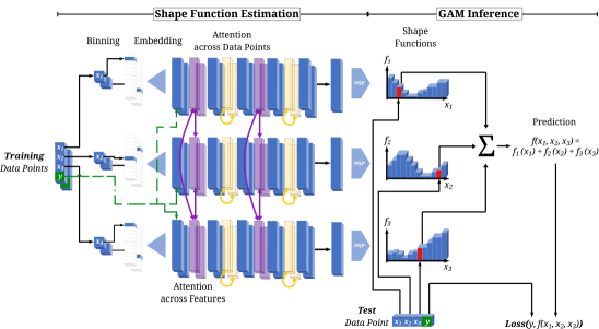
We introduce GAMformer (see  Figure 1), the first GAM method to estimate shape functions using ICL in a single forward pass. GAMformer distinguishes itself from existing GAM methods by employing a non-parametric, binned representation of shape functions, thus eliminating the need to impose a specific model class. Similar to TabPFN, our model is trained exclusively on large-scale synthetic datasets, yet demonstrates robust performance on real-world data. During training, GAMformer estimates shape functions for each feature based on the training data’s features and labels. These estimated functions are then utilized to generate predictions for test data points by summing the shape function values across features. The model is trained end-to-end based on the GAM’s predictions, ensuring that it learns to accurately construct shape functions for reliable predictions.

Figure 1: GAMformer’s forward pass on a new dataset with three features ($x_{1}$, $x_{2}$, $x_{3}$) and label $y$ and two data points: (1) For each data point, we bin all features, one-hot encode them, embed the resulting vectors and add the label of the data point. (2) We alternate between applying attention across the features and the data points, allowing us to handle varying numbers of each. (3) We decode per-feature shape functions using a shared MLP decoder. (4) We infer the prediction for test data points by looking up and adding each feature’s shape function value (red bins) forming the GAM prediction. (5) Finally, we compute the loss based on the prediction allowing the end-to-end training of the shape function estimation based on (in our case, synthetic) training datasets.

Our main contributions can be summarized as follows:

• We introduce GAMformer, the first method to utilize in-context learning with sequence-to-sequence models to form shape functions in a single forward pass, eliminating the need for iterative learning and hyperparameter tuning.

• Our experimental results demonstrate GAMformer’s capacity to match the accuracy of leading GAMs on various classification benchmarks.

• Our case study on MIMIC-II demonstrates how GAMformer can be applied to real-world data to generate interpretable models and insights of that data.

2 Background and Related Work

In this section, we provide some background and related work on generalized additive models and in-context learning.

2.1 Generalized Additive Models.

Generalized Additive Models (GAMs) (Hastie and Tibshirani, 1987) emerged as a generalization of Generalized Linear Models (Nelder and Wedderburn, 1972) which include non-linear transformations of the input features. The structure of a GAM is given by:

$$g(\mathbb{E}[y|x])=\beta+\sum\nolimits_{i=1}^{p}f_{i}(x_{i}),$$ (1)

where $x=(x_{1},\dots x_{p})\in\mathcal{X}\subseteq\mathbb{R}^{p}$ is the input with $p$ features, $y\in\mathcal{Y}\subseteq\mathbb{R}^{m}$ is the response variable, and $f_{i}:\mathbb{R}\to\mathbb{R}$ are univariate functions termed shape functions that capture the individual contributions of each feature. The intercept $\beta\in\mathbb{R}$ is a learnable bias term, and $g:\mathbb{R}\to\mathbb{R}$ is the link function that connects the expected outcome to the linear predictor, examples of which include the logit or softmax function for binary or multiclass classification or the identity function for linear regression. The shape functions $f_{i}$ in GAMs, also sometimes called partial dependence plots, allow for an interpretable representation of each feature’s effect, akin to the role of coefficients in linear regression, thus enabling practitioners to inspect the learned potentially non-linear relationships.

Traditional GAMs often use splines and backfitting (Hastie and Tibshirani, 1987), enhanced by penalized regression splines (Wood, 2003) and fast fitting algorithms (Wood, 2001). Spline-based GAMs use the backfitting algorithm, iteratively updating each shape function to fit the residuals of others until convergence. More recent advances include Explainable Boosting Machines (EBMs) (Lou et al., 2012; 2013; Caruana et al., 2015), which use decision trees to model shape functions via cyclic gradient boosting. This approach learns each feature’s contribution iteratively in a round-robin manner, mitigating collinearity effects and accurately modeling steps in the data, which is crucial for capturing discontinuities like treatment effects in medical data. On the other hand, Neural Additive Models (NAMs) (Agarwal et al., 2021) and follow up works (Chang et al., 2021; Dubey et al., 2022; Radenovic et al., 2022; Xu et al., 2022; Enouen and Liu, 2022; Bouchiat et al., 2024) use multilayer perceptrons (MLPs) as non-linear transformations to model the shape functions $f_{i}$. As a result, NAMs can be optimized using variants of gradient descent by leveraging automatic differentiation frameworks. Finally, GAMs have also found applications in time-series forecasting, with models such as Prophet (Taylor and Letham, 2018) and NeuralProphet (Triebe et al., 2021). For a more comprehensive related work refer to Appendix A.

2.2 In-Context Learning & Prior-Data Fitted Networks

In-Context Learning (ICL) was first demonstrated alongside the introduction of GPT-3 (Brown et al., 2020b), where the authors showed that Transformer models (Vaswani et al., 2017) could learn to perform tasks solely from input examples, without explicit training or fine-tuning, after self-supervised pre-training. This capability marks a significant paradigm shift from the traditional machine learning paradigm of in-weights learning, where the parameters of a model are adjusted in order to learn a new task. The discovery of ICL has led to numerous investigations into the mechanisms used by trained transformers that enable ICL. Olsson et al. (2022) found that a two-layer attention-only network can develop “induction heads”, a mechanism that outputs the token succeeding a previous instance of the current token, precisely when its ICL performance increases. Chan et al. (2022) investigated the properties of the data that contribute to the emergence of ICL abilities, while Reddy (2024) identified factors responsible for the abrupt emergence of induction heads.

Of particular relevance to this paper are Prior-Data-Fitted Networks (PFNs) (Müller et al., 2022; Hollmann et al., 2023), which showed that a transformer trained on complex synthetic data generated using random causal graphs can be used for tabular classification. From a Bayesian perspective, such causal graphs $\phi$ sampled from a hypothesis space $\Phi$ (the prior), define a mechanism that describes the relationship between the input and output variables. In TabPFNs (Hollmann et al., 2023), a synthetic dataset $D\sim p(D)=\mathbb{E}_{\phi\sim p(\phi)}[p(D|\phi)]$ is repeatedly constructed by propagating samples $x\sim p(\mathcal{X})$ from the input space through a randomly sampled structural causal model (SCM), $\phi\sim p(\phi)$, to obtain the corresponding $y$ values. We denote the dataset containing $N$ such examples as the set $D:=\{(x^{(n)},y^{(n)})\}_{n=1}^{N}$. To simulate practical inference scenarios, the dataset $D$ is split into $D_{\text{train}}$ and the context dataset $D_{\text{test}}=D\setminus D_{\text{train}}$. The transformer model parses the pairs $(x_{\text{train}},y_{\text{train}})\in D_{\text{train}}$, as well as $x_{\text{test}}$, as single input tokens and its parameters $\theta$ are updated to minimize the negative log likelihood on the test held-out examples:

$$\mathbb{E}_{(D_{\text{train}}\cup(x_{\text{test}},y_{\text{test}}))\sim p(D)}[-\log q_{\theta}(y_{\text{test}}|x_{\text{test}},D_{\text{train}})].$$ (2)

Müller et al. (2022) showed that by minimizing this loss, TabPFN approximates the true posterior predictive distribution

$$p(y_{\text{test}}|x_{\text{test}},D_{\text{train}})=\int_{\Phi}p(y_{\text{test}}|x_{\text{test}},\phi)p(\phi|D_{\text{train}})d\phi\propto\int_{\Phi}p(y_{\text{test}}|x_{\text{test}},\phi)p(D_{\text{train}}|\phi)p(\phi)d\phi$$ (3)

on a new input point from the test set $x_{\text{test}}$ up to an additive constant. This paradigm has since been extended to time-series forecasting (Dooley et al., 2024), hyperparameter optimization (Müller et al., 2023a; Adriaensen et al., 2024; Rakotoarison et al., 2024) and the prediction of neural network weights (Müller et al., 2023b). Similarly, Conditional Neural Processes (Garnelo et al., 2018) also perform a form of ICL, using a neural architecture with weights meta-learned on real data. (Nguyen and Grover, 2022) extended Neural Processes to a transformer architecture, leading to an architecture similar to PFNs. GAMformer builds on top of TabPFN by training a transformer on synthetically generated datasets to estimate the shape function per feature and computing predictions by adding the individual shape function values.

3 GAMformer

We first provide a high-level overview of how GAMformer works before delving into the details of each of its components. GAMformer follows a two-step approach that first fits a GAM on training data $D_{\text{train}}$ and then predicts on test data $x_{\text{test}}$, as illustrated in Figure 1. Initially, a transformer estimates shape functions using ICL on the training dataset $D_{\text{train}}$. Next, predictions are computed by aggregating the shape function values for each test data point $x_{\text{test}}$. This methodology replaces the traditional data fitting process of GAM variants with a single forward pass of a pre-trained transformer model, eliminating the need for optimization and regularization hyperparameters. We now describe each model component in more detail.

3.1 Shape Estimation and Predictions

We obtain the shape functions with ICL by applying a transformer on the training input points and labels:

$$\tilde{f}=\mathcal{T}_{\theta}(x_{\text{train}},y_{\text{train}})\in\mathbb{R}^{p\times n_{\text{bins}}\times m},$$ (4)

where $p,m$ and $n_{\text{bins}}$ are respectively the numbers of features, classes and bins. To get predictions on a new test point $x_{\text{test}}$, we first bin each feature value and then apply the estimated shape function:

$$g\left(\tilde{y}_{\text{test}}\right)=\sum_{i=1}^{p}\tilde{f}_{ij_{x_{i}}}\in\mathbb{R}^{m},$$ (5)

where $j_{x_{i}}\in[n_{\text{bins}}]$ denotes the bin index corresponding to the $i-$th feature of $x_{\text{test}}$. We now give more details on the binning and the architecture used for $\mathcal{T}_{\theta}$ in Eq. 4 before discussing the pre-training.

3.2 Model Architecture

Feature Preprocessing.

Prior to being passed through the transformer, all features of each data point are binned, one-hot encoded, and finally embedded using an MLP. We use $n_{\text{bins}}=64$ bins for each feature, allocating bins based on the quantiles of the feature in the training dataset. Similarly to TabPFN, we embed the label of each datapoint and add it to the embedding of each feature. Categorical features are equally distributed across the 64 bins according to their ratios.

Representation of the shape functions.

To accurately represent the shape functions, we chose to predict a discrete representation for each feature by discretizing it into 64 bins. An alternative approach would have been to predict the weights of a Neural Additive Model (NAM), similar to the method employed by Mothernet (Müller et al., 2023b). However, we decided against this approach to more naturally represent sudden discontinuities in the shape functions.

Transformer.

The preprocessed training datapoints are processed by a transformer architecture consisting of 12 layers, each with a dual-module design that sequentially applies self-attention—first over the features and then over the data points. This design, inspired by (Lorch et al., 2022), ensures that our model is agnostic to the number of features and data points, and is equivariant with respect to the order of both. As a result, unlike TabPFN (Hollmann et al., 2023), our approach does not require padding to a fixed maximum number of features.

After the transformer layers, we compute the average embeddings for each class based on training labels enabling multi-class classification (limited to 10 classes in our experiments). This averaging yields one embedding per class per feature which we denote $h\in\mathbb{R}^{p\times d\times m}$ where $d$ denotes the embedding dimension of the transformer. Each embedding is then passed through a shared decoder MLP to produce the binned shape functions $\tilde{f}\in\mathbb{R}^{p\times n_{\text{bins}}\times m}$. This architecture is parameter-efficient as it allows sharing of parameters across features and classes. The model comprises 40k parameters in the encoder layer, 50.5M parameters in the transformer layers, and 0.3M parameters in the decoder, resulting in a total of 50.8M parameters. Note that while the shape function estimation scales quadratically in the number of features and datapoints, the inference only scales linearly in both.

3.3 Training Procedure

We train with SGD on synthetic data priors, a method introduced in Prior-Data Fitted Networks (PFNs) (Müller et al., 2022; Hollmann et al., 2023). These priors are designed to be diverse, facilitating the generation of realistic tabular datasets and enabling extrapolation to real-world data. We utilize two types of priors for training: (1) Structural Causal Models, which involve sampling random causal graphs and generating data from them, and (2) Gaussian Processes, where random Gaussian Processes are sampled and used to generate data. For more details on the synthetic data generation process, we refer to Appendix D. During training, the synthetic data is randomly split into train and test datasets. To obtain the parameters $\theta$ of Eq. 4 we minimize a cross-entropy loss between the estimated GAM prediction and ground truth labels on the test dataset $D_{\text{test}}$:

$$\theta^{*}\in\text{argmin}_{\theta}\mathbb{E}_{(D_{\text{train}}\cup(x_{\text{test}},y_{\text{test}}))\sim p(D)}\left[\mathcal{L}(\tilde{y}_{\text{test}},y_{\text{test}})\right]$$ (6)

Additional details on the training are given in Appendix E.

GAMformer’s core contribution is the substitution of the data fitting process of traditional GAM variants with a single forward pass of a pre-trained transformer model, which is presented with data through in-context examples. Consequently, GAMformer replaces the manually crafted fitting procedures used in methods like EBMs (Caruana et al., 2015), where the boosting procedure is restricted to one feature at a time in a round-robin manner, or the joint optimization of all shape functions in NAMs (Agarwal et al., 2021) using SGD. Note that in both traditional GAM fitting and GAMformer, the output of the processes remains the same; a main effects GAM fitted to a given dataset represented by its shape functions.

3.4 Higher-order effects

We now describe how GAMformer can be extended to handle higher-orders effects. We extend GAMformer to model higher-order effects, specifically pairwise interactions, by incorporating feature products, resulting in up to $\mathcal{O}(p^{2})$ potential features. GAMformer can accommodate this by performing ICL on concatenated original data and higher-order effects, represented as feature vectors in $\mathbb{R}^{p+P}$, where $P$ denotes the number of pair interactions. However, increasing feature dimensions beyond the $10$ used in pretraining is problematic and adds complexity to shape function estimation. To mitigate this, we rank the most informative pairs via the FAST method (Lou et al., 2013) and the optimal number of pairs is determined as a hyperparameter through cross-validation during inference.

4 Experiments

After pretraining GAMformer on the synthetic datasets, we evaluate it on both illustrative and real-world tasks in 4.1 and 4.2, respectively. Moreover, in 4.3, we highlight its potential to assist in decision-making in a clinical setting by predicting the mortality rate of patients in the intensive care unit (ICU). We compare to Explainable Boosting Machines (EBMs) (Lou et al., 2012; 2013; Caruana et al., 2015) in terms of estimated shape function quality, as well as to other state-of-the-art tabular classification models such as XGBoost (Chen and Guestrin, 2016) and TabPFN (Hollmann et al., 2023) in terms of predictive performance. On the downstream datasets, differently from EBM and the other baselines, GAMformer requires only a single forward pass of the transformer model to estimate the shape functions and construct prediction on the entire test set, without any parameter updates.

4.1 Illustrative Examples

Figure 2: Shape functions derived from GAMformer and EBMs applied to the linear, binary classification problem $f(x_{1},x_{2},x_{3})=\mathbb{I}((-1)x_{1}+0x_{2}+x_{3}>0)$. We use a twin y axis with GAMformer and EBM on left and right, respectively. All models shown result from a 30-fold cross-validation over 1500 data points.

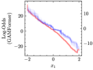
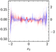
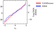
Before demonstrating GAMformer on real-world tabular data, we first investigate its behavior on synthetic data where the data-generation process is known. This allows us to validate the effectiveness of GAMformer in capturing the underlying relationships between features and the target variable. All considered examples are binary classification and hence we only show one shape function per class and per feature. In the context of GAMs with a logit link function (used for binary classification), log-odds is the unit of the predictors. Therefore, the shape functions’ output values are on the log-odds scale, which are then transformed to overall prediction probabilities after summing via the logistic function. For all metrics reported in the paper, we use ROC-AUC (Receiver Operating Characteristic - Area Under the Curve).

Figure 3: Robustness analysis (linear, binary classification): GAMformer consistently outperforms or matches EBM across various sample sizes and feature counts, showcasing its efficiency

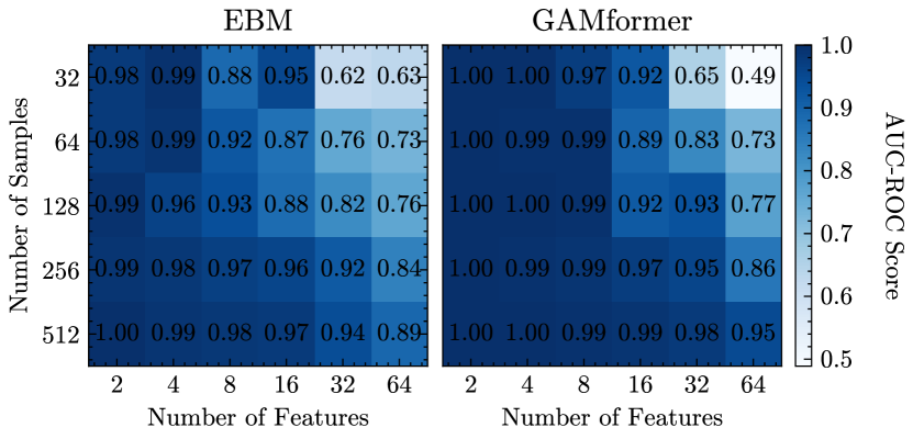
Linear, binary classification. We begin by evaluating GAMformer and, for comparison, EBMs on data generated by the linear, binary classification problem $f(x_{1},x_{2},x_{3})=\mathbb{I}((-1)x_{1}+0x_{2}+x_{3}>0)$, where $\mathbb{I}$ is the indicator function. We sample 2000 data points uniformly and independently from the interval [-2, 2] and split the data into 1500 training points and 500 test points. The results, shown in Figure 2, demonstrate that both GAMformer and EBMs accurately estimate the slopes for each feature and achieve an ROC AUC of 1.0 on the test dataset. However, the shape functions learned by GAMformer are noticeably smoother, suggesting that it may have captured some bias towards smoother models during pretraining. Additionally, we compared the effect of varying the number of datapoints or features in this example on EBMs and GAMformer in Figure 3. Our findings indicate that GAMformer consistently outperforms EBMs across various sample sizes and feature counts.

Figure 4: (a) Shape functions derived from GAMformer and EBMs applied to the polynomial, binary classification problem $f(x_{1},x_{2})=\mathbb{I}(x_{1}+x_{2}^{2}>0)$. All models result from a 30-fold cross-validation over 1500 data points are shown.

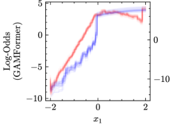
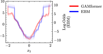
Polynomial, binary classification. To further validate the robustness of GAMformer, we evaluate it on data generated by a more complex function $f(x_{1},x_{2})=\mathbb{I}(x_{1}+x_{2}^{2}>0)$. The experimental setup remains the same as for the logistic regression case. The results, presented in Figure 4, show that both GAMformer and EBMs successfully capture the quadratic relationship in $x_{2}$ and the linear contribution of $x_{1}$ up to $x_{1}\leq 0$. For $x_{1}>0$, $f$ always predicts true, resulting in a constant contribution. Consistent with the previous experiment, GAMformer produces smoother shape functions. Again both models achieve an ROC AUC of 1.0 on the test dataset.

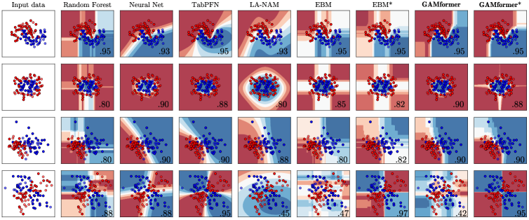
Classification Boundaries. We visualize the classification boundaries of GAMformer compared to TabPFN and EBM on the scikit-learn (Pedregosa et al., 2011) test datasets in Figure 5. We find that GAMformer performs similarly to TabPFN and EBMs on most of the example datasets. LA-NAM (Bouchiat et al., 2024) (main effects only), a Bayesian version of NAMs (Agarwal et al., 2021), provides good uncertainty estimates despite exhibiting slightly worse predictive performance. It is worth noting that GAMformer, EBM and LA-NAM struggle with accurately modeling the ‘XOR’ dataset (bottom row) due to the absence of higher-order feature interaction terms in these models. This is resolved by incorporating second-order effects (EBM^∗ and GAMformer^∗; see Section 3.4 for details), allowing them to effectively learn the non-linear decision boundary of the ‘XOR’ function.

Figure 5: Visualization of classification boundaries for various baseline classifiers and GAMformer on scikit-learn dataset examples (Pedregosa et al., 2011), in the lower right corner we show the ROC-AUC on a validation split. Due to the absence of higher-order feature interaction terms in both GAMformer and EBM (main effects), the ’XOR’ dataset (bottom row) is not accurately modeled by them. Incorporating second-order effects solves the problem (EBM^∗ and GAMformer^∗).

4.2 Multi-class Classification on OpenML Tabular Datasets

To assess the transferability of pretraining on synthetic data to real-world tabular data, we evaluate GAMformer’s performance on the test datasets from TabPFN (Hollmann et al., 2023), which include up to 2000 datapoints (see Section B.1 for dataset details). Figure 6 reports Critical Diagrams (CD) from Demšar (2006) showing the average rank across datasets for each method, with statistically tied methods grouped by horizontal bars. Our method outperforms EBM when using only main effects. With pair effects, both GAMformer* and EBM* show slight improvements, matching XGBoost’s performance. We also compare against GAMs from the mgcv R  library. mgcv GAM models the relationships between features and output variables by combining parametric and non-parametric terms. The non-parametric components are represented by splines, thus capturing nonlinear relationships. In mgcv GAM the degree of smoothness in every spline is automatically selected using Restricted Maximum Likelihood (REML) (Wood, 2010).

We note that the small difference in performance between XGBoost and GAMformer suggests that the trade-offs in model capacity when choosing a main effects only GAM are often less significant than expected. As a result, the substantial interpretability benefits offered by the GAM model class become even more appealing, making it a viable choice for many applications. We present additional results on five binary classification datasets used by Chang et al. (2021) in Section B.2. Despite these datasets falling outside the recommended range of 2000 datapoints, GAMformer still demonstrates comparable performance to more complex models.

4.3 Case Study: Intensive Care Unit Mortality Risk

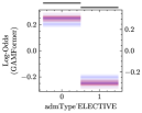
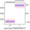
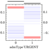
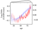
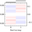
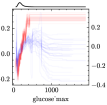
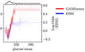
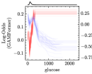
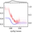
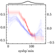
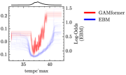
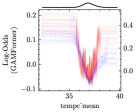
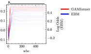
In this case study, we examine shape functions derived from GAMformer and EBMs (main effects only) using the MIMIC-II dataset (Lee et al., 2011a), a publicly available critical care dataset for predicting mortality risk based on various demographic and biophysical indicators. Our analysis focuses on four key clinical variables: Age, Heart Rate (HR), PFratio (PaO2/FiO2 ratio), and Glasgow Coma Scale (GCS), as shown in Figure 7 (remaining variables in Section G.1). Further results on the MIMIC-III dataset are available in Section G.2.

Figure 6: Critical Difference diagram demonstrating GAMformer’s competitive performance against state-of-the-art baselines across diverse datasets. Lower ranks indicate superior performance; connected algorithms are not statistically significantly different ($p=0.05$).

Figure 7: Shape functions derived from GAMformer and EBMs applied to the MIMIC-II dataset for critical clinical variables. The data density plot is shown above each figure. The results are based on 30 models for both GAMformer and EBMs, each fitted on 10,000 randomly selected data points.

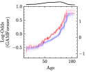
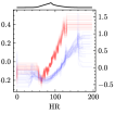
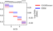
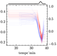
For Age, the GAMformer shape function shows a steady increase in the log-odds of adverse outcomes with advancing age, stabilizing at older ages. The data density plot reveals a higher concentration of data points in middle age, with fewer at the extremes. The shape function exhibits less variance where data is denser, indicating the model’s reliability in these regions. Overall, the shape function highlights increased risk in elderly patients due to declining physiological reserves and multiple chronic conditions. Heart Rate (HR) exhibits a complex relationship with adverse outcomes. Both GAMformer and EBMs capture a U-shaped risk profile, indicating increased risk at very high and very low heart rates, underscoring the importance of maintaining HR within a normal range. PFratio, a lung function and oxygenation efficiency measure, shows a steep risk increase as values decrease. Lower PFratio values, critical in diagnosing and managing conditions like Acute Respiratory Distress Syndrome (ARDS), indicate worse lung function. Notably, both models display a sharp drop in risk at a PFratio of approximately 325, likely an artifact from data preprocessing where missing values were imputed at the mean, previously pointed out by Chen et al. (2023) for MIMIC-2. In healthcare, missing values often suggest healthier patients, as data collection was deemed unnecessary by professionals. Here, patients with missing PFratio values, representing the majority, have lower risk than those with collected values. GAMformer more precisely isolates these missing value patients, demonstrating its potential to detect data processing artifacts better than prior GAM algorithms. For the Glasgow Coma Scale (GCS), which measures the level consciousness, there is a strong negative correlation with adverse outcomes. Lower GCS scores, indicating reduced consciousness, are associated with significantly higher mortality risk. Our findings show that GAMformer effectively handles categorical data, identifying patterns similar to those detected by EBMs.

5 Limitations & Broader Impact

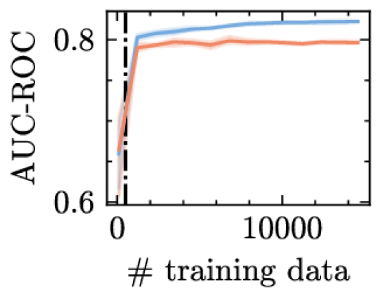
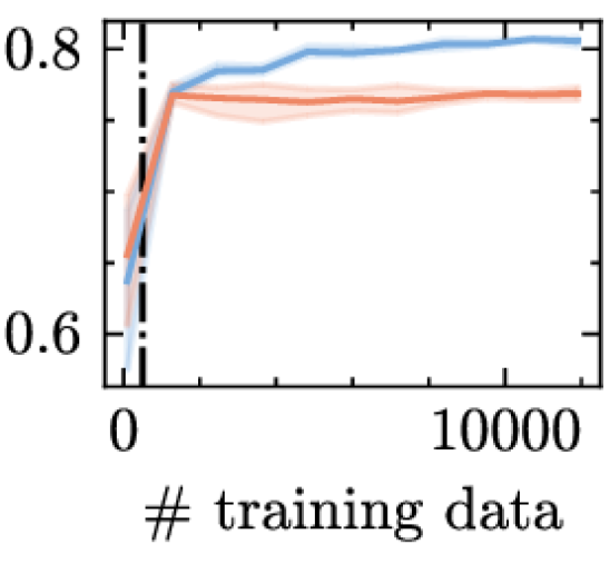
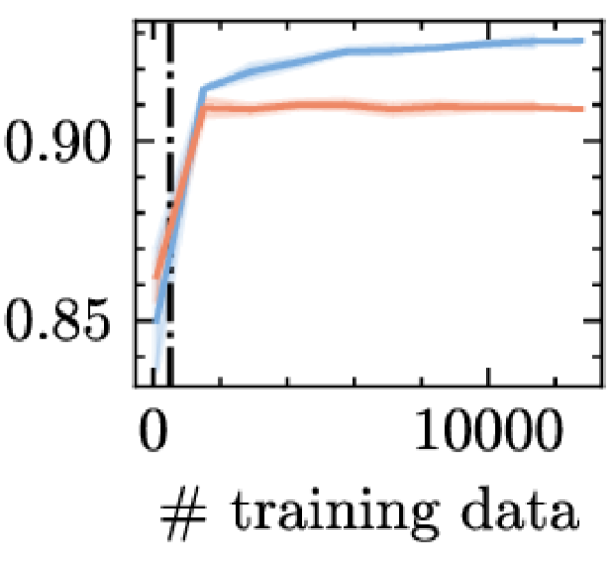
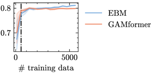
Limitations. While GAMformer introduces a novel approach to estimating Generalized Additive Models (GAMs), it is important to acknowledge its current limitations. This work primarily focuses on main and second-order effect GAMs and does not account for higher-order interactions, which are addressed in other GAM implementations, such as EBMs (Lou et al., 2013; Nori et al., 2019; Chang et al., 2021). Future research could explore incorporating these interactions to enhance the model’s expressiveness and predictive capabilities. Another limitation of the current GAMformer model is its difficulty in improving predictions when presented with datasets that exceed twice the size of the data it saw during training (c.f. Figure 8). This issue is related to the well-known challenge of length extrapolation in sequence-to-sequence models, including transformers (Grazzi et al., 2024; Zhou et al., 2024). Addressing this limitation may require exposing the model to a larger variety of number of examples during training. However, due to computational constraints, the experiments in this work were limited to a maximum of 500 datapoints during training. Future studies with increased computational resources could investigate the model’s performance on larger datasets and develop strategies to mitigate the length extrapolation problem. The GAMformer model’s transformer-based architecture scales quadratically with both the number of training data points and features, posing a similar challenge to handling large datasets as faced by TabPFN (Hollmann et al., 2023). Novel, scalable transformer alternatives, such as the recently proposed Mamba (Gu and Dao, 2023) or Gated Linear Attention (Yang et al., 2024), may prove useful in overcoming this issue.

Broader Impact. As a versatile machine learning model for tabular data, GAMformer offers both positive and negative societal impacts. Positively, it can generate novel insights in fields like medicine, enhancing disease diagnosis and treatment. However, it can also be misused to not mitigate but exploit biases, such as adjusting insurance premiums based on ethnicity, leading to discrimination.

6 Conclusion

In this paper, we introduce GAMformer, a novel approach to creating GAMs using in-context learning with transformer models. By leveraging a single forward pass to form shape functions, GAMformer overcomes the limitations of traditional GAM algorithms that require iterative learning processes and hence hyperparameter tuning. Our approach uses non-parametric, binned representations of shape functions, resulting in significant improvements in efficiency and accuracy across various classification benchmarks. Extensive experiments demonstrate that GAMformer approaches the accuracy of leading GAM variants while exhibiting robustness to label noise and class imbalance. The model’s ability to generalize beyond the number of examples seen during training highlights its adaptability and potential for practical applications.

GAMformer is fundamentally different from the iterative optimization methods traditionally used, and offers a new research direction for interpretable models on tabular data. Further, our case study on the MIMIC-II dataset showcases that interpreting GAMformer’s shape functions can yield qualitative insights and uncover flaws in datasets similar to state of the art GAM methods. This work contributes to the development of more transparent and explainable AI systems, with potential applications in various domains where interpretability is crucial. Future research can expand on this initial new paradigm, and explore scalable alternatives to transformers to handle larger datasets.

Appendix A Generalized Additive Models: Extended Related Work

As with many families of machine learning algorithms, the differences among GAM algorithms lie in (a) the functional form of the shape functions $f_{i}$, (b) the learning algorithm used for their estimation and (c) regularity assumptions and regularization. Two important properties that all GAMs share are (1) the ability to learn non-linear transformations for each feature and (2) additively combining these shape functions (prior to applying the link function) to create modularity that aids interpretability by allowing users to examine shape functions one-at-a-time.

Typically, GAMs have relied on splines and backfitting algorithms for estimation [Hastie and Tibshirani, 1987], with subsequent works focusing on improving efficiency and stability through penalized regression splines [Wood, 2003] and fast, stable fitting algorithms [Wood, 2001]. Spline-based GAMs are typically fitted using the backfitting algorithm, an iterative procedure that starts with initial estimates of the smooth functions for each predictor variable. The algorithm then repeatedly updates each function by fitting a weighted additive model to the residuals of the other functions until convergence is achieved. The weights are determined by the current estimates of the other functions and the link function in the case of generalized additive models.

Modern approaches leverage machine learning advances. Explainable Boosting Machines (EBMs) [Lou et al., 2012, 2013, Caruana et al., 2015] model the shape functions using decision trees, which are fitted using a variant of gradient boosting called cyclic gradient boosting. The model iteratively learns the contribution of each feature and interaction term in a round-robin fashion, using a low learning rate to ensure that the order of features does not affect the final model. This cyclic training procedure helps mitigate the effects of colinearity among predictors by providing opportunity for data-driven credit attribution among the features while preventing multiple counting of evidence. EBMs are also popular because they can accurately capture steps in the shape functions, which is important for modeling discontinuities in data, such as treatment effects in medical data.

More recently, Neural Additive Models (NAMs) [Agarwal et al., 2021] and follow up works [Chang et al., 2021, Dubey et al., 2022, Radenovic et al., 2022, Xu et al., 2022, Enouen and Liu, 2022, Bouchiat et al., 2024] use multilayer perceptrons (MLPs), as non-linear transformations, to model the shape functions $f_{i}$. As a result, NAMs can be optimized using variants of gradient descent by leveraging automatic differentiation frameworks.

Finally, GAMs have also found applications in time-series forecasting, with models such as Prophet [Taylor and Letham, 2018] and NeuralProphet [Triebe et al., 2021]. Interestingly, the 1-layer versions of the recently proposed Kolmogorov-Arnold Networks (KANs) [Liu et al., 2024] may be viewed as GAMs with spline based shape functions.

Appendix B Dataset Details

In this section, we provide details on the datasets used in our empirical evaluations of GAMformer and other baselines in Section 4 of the main paper.

B.1 TabPFN Test Datasets

As test dataset, we used the 30 datasets used in Hollmann et al. [2023] which were obtained from OpenML [Vanschoren et al., 2014]. These were chosen because they contain up to 2000 samples, 100 features and 10 classes, show in Table 1.

Table 1: Test dataset names and properties, taken from Hollmann et al. [2023]. Here did is the OpenML Dataset ID, d the number of features, n the number of instances, and k the number of classes in each dataset.

did	name	d	n	k
11	balance-scale	5	625	3
14	mfeat-fourier	77	2000	10
15	breast-w	10	699	2
16	mfeat-karhunen	65	2000	10
18	mfeat-morphological	7	2000	10
22	mfeat-zernike	48	2000	10
23	cmc	10	1473	3
29	credit-approval	16	690	2
31	credit-g	21	1000	2
37	diabetes	9	768	2
50	tic-tac-toe	10	958	2
54	vehicle	19	846	4
188	eucalyptus	20	736	5
458	analcatdata_authorship	71	841	4
469	analcatdata_dmft	5	797	6

did	name	d	n	k
1049	pc4	38	1458	2
1050	pc3	38	1563	2
1063	kc2	22	522	2
1068	pc1	22	1109	2
1462	banknote-authentication	5	1372	2
1464	blood-transfusion-…	5	748	2
1480	ilpd	11	583	2
1494	qsar-biodeg	42	1055	2
1510	wdbc	31	569	2
6332	cylinder-bands	40	540	2
23381	dresses-sales	13	500	2
40966	MiceProtein	82	1080	8
40975	car	7	1728	4
40982	steel-plates-fault	28	1941	7
40994	climate-model-…	21	540	2

B.2 Binary Classification

Table 2: Comparison of GAMformer with other GAM variants and full complexity models on various datasets. We report ROC-AUC (%) (higher is better) and the standard error over 10 fold cross-validation. We also report results by pyGAM [Servén and Brummitt, 2018].

	GAMs					Full Complexity
	GAMformer (ours)	EBM (Main effects)	Logistic Regression	pyGAM (Main effects)	EBM	XGBoost	Random Forest
Churn	81.69 $\pm$ 0.1	83.59 $\pm$ 0.1	81.66 $\pm$ 0.1	82.03 $\pm$ 0.0	83.68 $\pm$ 0.1	83.53 $\pm$ 0.0	82.07 $\pm$ 0.0
Support2	80.84 $\pm$ 0.1	82.36 $\pm$ 0.0	81.1 $\pm$ 0.0	81.74 $\pm$ 0.2	83.51 $\pm$ 0.0	84.03 $\pm$ 0.0	83.93 $\pm$ 0.0
Adult	90.05 $\pm$ 0.0	93.05 $\pm$ 0.0	90.73 $\pm$ 0.0	91.55 $\pm$ 0.0	93.07 $\pm$ 0.0	93.16 $\pm$ 0.0	91.8 $\pm$ 0.0
MIMIC-2	82.22 $\pm$ 0.0	85.15 $\pm$ 0.0	81.62 $\pm$ 0.0	83.89 $\pm$ 0.1	86.36 $\pm$ 0.1	87.29 $\pm$ 0.0	87.31 $\pm$ 0.0
MIMIC-3	74.41 $\pm$ 0.1	81.14 $\pm$ 0.0	78.05 $\pm$ 0.0	79.95 $\pm$ 0.1	82.52 $\pm$ 0.1	83.32 $\pm$ 0.0	81.28 $\pm$ 0.1

Churn dataset.

The Telco Customer Churn Dataset is a binary classification dataset for predicting potential subscription churners in a telecom company, containing customer information and churn-related features.

Adult dataset.

The Adult dataset Dua and Graff [2017], also known as the “Census Income” dataset, is a widely-used benchmark for binary classification, predicting whether an individual’s annual income exceeds $50,000 based on 14 attributes from the 1994 United States Census Bureau data.

MIMIC-II dataset.

The MIMIC-II dataset Lee et al. [2011b] is a publicly-available database of clinical data from diverse ICU patients, integrating demographics, vital signs, lab results, medications, procedures, notes, and imaging reports, along with mortality outcomes.

MIMIC-III dataset.

The MIMIC-III dataset Johnson et al. [2016] expands on MIMIC-II, with a larger patient cohort, more recent records, enhanced data granularity, and the inclusion of free-text imaging report interpretations.

SUPPORT2 dataset.

The SUPPORT2 dataset Connors Jr et al. [1996] contains medical information from critically ill hospitalized adults, compiled to study the relationships between medical decision-making, patient preferences, and treatment outcomes, with variables spanning demographics, physiology, diagnostics, treatments, and survival/quality of life outcomes.

Appendix C Properties of GAMformer

C.1 Data Scaling

To assess GAMformer’s ability to generalize to datasets containing more datapoints than it saw during training, i.e. larger context sizes, we conducted an experiment that varied the number of training data points and evaluated the impact on ROC-AUC performance using a consistent validation split. To ensure the robustness of our findings, we sampled training datasets three times with replacement for each training size. The results in Figure 8 demonstrate that GAMformer’s ROC-AUC improves across datasets when the number of training examples is up to twice the number of training examples seen during training. For comparison, we also evaluated the performance of EBMs under the same conditions. While EBMs also exhibited improvements in ROC-AUC with increased training data, they achieved higher accuracy when provided with a larger number of examples. This observation highlights a limitation of GAMformer in its ability to fully leverage additional training samples.

(a) MIMIC-II

(b) MIMIC-III

(c) Adult

(d) Support 2 ———————

Figure 8: Demonstration of the ability of GAMformer to scale beyond the datapoints seen during training while leveraging the additional data points to increase its performance. The dashed vertical line denotes the number of in-context examples seen during training (500).

C.2 Class Imbalance

(a) Imbalanced Data

(b) Noisy Labels —————

Figure 9: Comparison of GAMformer and EBMs in terms of (a) performance on class imbalanced data and (b) robustness to noisy labels. The shaded areas represent the 5% and 95% confidence intervals estimated using 1000 bootstrap samples.

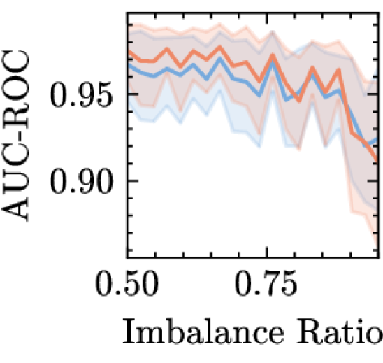
To compare GAMformer’s sensitivity to class imbalance with that of EBMs, we conduct the following analysis. First, we sample 300 data points from two centroids in a 20-dimensional feature space, creating a binary classification problem. We then vary the ratio of the two classes to introduce increasing levels of imbalance in the sampled data. Next, we split the data into train and test sets using a 75% to 25% split and evaluate the performance using the AUC-ROC metric. We repeat the experiment 10 times for each data ratio. Our results are shown in Figure 9(a), the shaded area are the 5%, 95% confidence intervals estimated using 1000 bootstrap samples. We see that GAMformer performs on average better than EBMs in this setting and shows no inherent sensitivity to class imbalance.

C.3 Noise Robustness

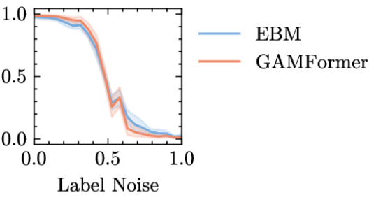
To gain a deeper understanding of GAMformers’ sensitivity to noisy or incorrect labels, we conducted an experiment similar to the one described in Section C.2. We generated 300 data points and randomly perturbed the labels in the train split with increasing probability (75%, 25% train/test split), repeating each experiment 10 times. Figure 9(b) illustrates our findings. Once again, we observed that GAMformer exhibits a sensitivity to noisy labels comparable to that of EBMs.

Appendix D Synthetic Data Priors

We use the same synthetic data generation process proposed in Prior-Data-Fitted Networks (PFNs) [Hollmann et al., 2023, Müller et al., 2022] and provide a brief summary of the process.

TabPFN is trained on two synthetic data priors, which are mixed during training.TabPFN introduced a synthetic data prior based on Structural Causal Models (SCMs). SCMs are particularly suitable for modeling tabular data as they capture causal relationships between columns, a strong prior in human reasoning. An SCM comprises a set of structural assignments (mechanisms) where each mechanism is defined by a deterministic function and a noise variable, structured within a Directed Acyclic Graph (DAG). The causal relationships are represented by directed edges from causes to effects, facilitating the modeling of complex dependencies within the data. To instantiate a PFN prior based on SCMs, one defines a sampling procedure to create supervised learning tasks. Each dataset is generated from a randomly sampled SCM, including its DAG structure and deterministic functions. Nodes in the causal graph are selected to represent features and targets, and samples are generated by propagating noise variables through the graph. This process results in features and targets that are conditionally dependent through the DAG structure, capturing both forward and backward causation [Hollmann et al., 2023]. This allows for the generation of diverse datasets.

The second prior samples of synthetic data using Gaussian Processes (GPs) [Rasmussen and Williams, 2006] with a constant mean function and a radial basis function (RBF) kernel to define the covariance structure. Hyperparameters such as noise level, output scale, and length scale are sampled from predefined distributions to introduce variability. Depending on the configuration, input data points can be sampled uniformly, normally, or as equidistant points and the target column is generated by passing the input data through the GP. This prior gives the model the ability to learn smoother functions.

For multi-class prediction, scalar labels are transformed into discrete class labels by partitioning the scalar values into intervals corresponding to different classes, ensuring the synthetic data is suitable for imbalanced multi-class classification tasks.

Finally, both priors are combined by sampling batches of data from each prior with different probabilities during training. In all of our experiments we sampled from the SCM and GP prior with probability $0.96$ and $0.04$, respectively.

Appendix E Training Details

In GAMformer, we used a transformer model with 12 hidden layers, 512 embedding size and 4 heads per attention. To bin the shape functions and all features we used 64 bins. For training, we use the AdamW [Loshchilov and Hutter, 2019] optimizer ($\beta_{1}=0.9$) and cosine learning rate schedule with initial learning rate of 3e-5, 20 warm up epochs and minimum learning rate of 1e-8 for 25 days on a A100 GPU with 80Gb of memory. We used mixed precision training. Each epoch (arbitrarily) consists of 65536 synthetic datasets; the model trained for 1800 epochs, meaning it saw over 100M synthetic datasets. We used a batch size of 8, that we doubled at epoch 20, 50, 200 and 1000. Each synthetic dataset consisted of 500 samples that were split into training and test portions using using a uniform sampling of the training fraction, and used a number of features drawn uniformly between 1 and 10.

Appendix F Higher-order effects

To handle higher-order effects, we compute the best pairs with the FAST algorithm [Lou et al., 2013] and evaluate GAMformer on the top pairs using the following ratios of features:

$$\mathcal{P}=[0.01p,0.05p,0.1p,0.2p,0.4p,0.8p,0.9p]$$

where we recall that $p$ denotes the number of features. We round off each ratio to determine the number of target pair features, evaluate performance on hold-out validation data from the training set, and select the number of pairs with the best validation performance. The model is then fitted on the entire training dataset. This involves doing $|\mathcal{P}|+1$ forward passes, which is unproblematic as doing one forward pass is very fast, even on a CPU. One could also vectorialize all computations which we do not do given the low fitting time.

Appendix G Shape Functions

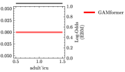
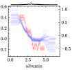
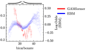
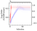
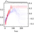
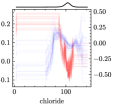
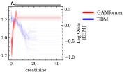
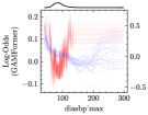
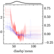
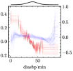
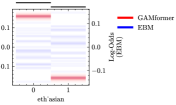
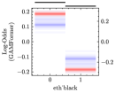
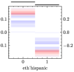
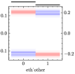
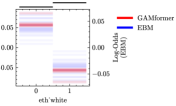
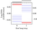
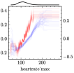
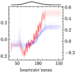
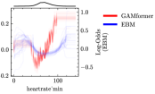
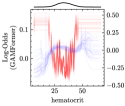
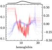
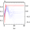
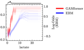
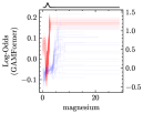
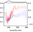
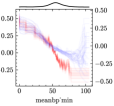
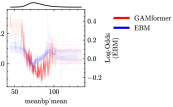
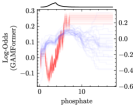
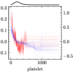
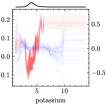
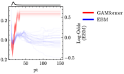
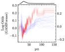
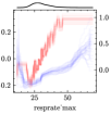
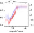
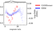
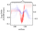
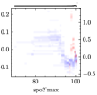
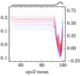
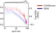
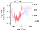
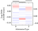
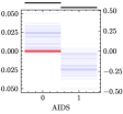
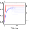
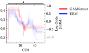
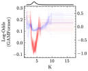
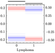
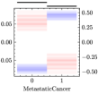
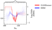
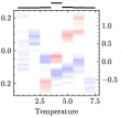
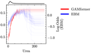
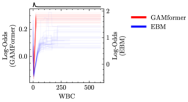
In this section, we show complementary results on the shape functions estimates from GAMformer and EBM (main effects only) on the MIMIC-II [Lee et al., 2011a] (complementary to the plots in Figure 7) and on the MIMIC-III datasets.

G.1 MIMIC-II dataset

Figure 10: The remaining shape functions derived from GAMformer and EBMs on the MIMIC-II dataset for critical clinical variables. The plot above each figure shows the data density. There are interesting differences between the EBM and GAMformer shape plots for several of the categorical variables. Although different GAM algorithms do not usually learn identical functions, we are investigating to better understand these differences.

G.2 MIMIC-III dataset

Figure 11: The shape functions derived from GAMformer and EBMs on the MIMIC-III dataset for critical clinical variables. The plot above each figure shows the data density. The results are based on 30 models for both GAMformer and EBMs, each fitted on 10,000 randomly selected data points. There are interesting differences between the EBM and GAMformer shape plots for several of the categorical variables. Although different GAM algorithms do not usually learn identical functions, we are investigating to better understand these differences.

Figure 12: The remaining shape functions derived from GAMformer and EBMs applied to the MIMIC-III dataset for critical clinical variables. The plot above each figure shows the data density in the training set. The results are based on 30 models for both GAMformer and EBMs, each fitted on 10,000 randomly selected data points.

References

- Barocas and Selbst [2016] Solon Barocas and Andrew D Selbst. Big Data’s Disparate Impact. California Law Review, pages 671–732, 2016.
- Rudin et al. [2022] Cynthia Rudin, Chaofan Chen, Zhi Chen, Haiyang Huang, Lesia Semenova, and Chudi Zhong. Interpretable Machine Learning: Fundamental Principles and 10 Grand Challenges. Statistic Surveys, 16:1–85, 2022.
- Ribeiro et al. [2016] Marco Tulio Ribeiro, Sameer Singh, and Carlos Guestrin. " why should i trust you?" explaining the predictions of any classifier. In Proceedings of the 22nd ACM SIGKDD international conference on knowledge discovery and data mining, pages 1135–1144, 2016.
- Caruana et al. [2015] Rich Caruana, Yin Lou, Johannes Gehrke, Paul Koch, Marc Sturm, and Noemie Elhadad. Intelligible models for healthcare: Predicting pneumonia risk and hospital 30-day readmission. In Proceedings of the 21th ACM SIGKDD International Conference on Knowledge Discovery and Data Mining, pages 1721–1730, 2015.
- Arun et al. [2016] Kumar Arun, Garg Ishan, and Kaur Sanmeet. Loan approval prediction based on machine learning approach. IOSR Journal of Computer Engineering, 18(3):18–21, 2016.
- Dattner et al. [2019] Ben Dattner, Tomas Chamorro-Premuzic, Richard Buchband, and Lucinda Schettler. The legal and ethical implications of using AI in hiring. Harvard Business Review, 25, 2019.
- Mehrabi et al. [2021] Ninareh Mehrabi, Fred Morstatter, Nripsuta Saxena, Kristina Lerman, and Aram Galstyan. A survey on bias and fairness in machine learning. ACM Comput. Surv., 54(6), jul 2021. ISSN 0360-0300. doi: 10.1145/3457607.
- Hastie and Tibshirani [1987] Trevor Hastie and Robert Tibshirani. Generalized Additive Models: Some applications. Journal of the American Statistical Association, 82(398):371–386, 1987.
- Lou et al. [2012] Yin Lou, Rich Caruana, and Johannes Gehrke. Intelligible Models for Classification and Regression. In Proceedings of the 18th ACM SIGKDD International Conference on Knowledge Discovery and Data Mining, pages 150–158, 2012.
- Lou et al. [2013] Yin Lou, Rich Caruana, Johannes Gehrke, and Giles Hooker. Accurate intelligible models with pairwise interactions. In Proceedings of the 19th ACM SIGKDD International Conference on Knowledge Discovery and Data Mining, pages 623–631, 2013.
- Agarwal et al. [2021] Rishabh Agarwal, Levi Melnick, Nicholas Frosst, Xuezhou Zhang, Ben Lengerich, Rich Caruana, and Geoffrey E Hinton. Neural Additive Models: Interpretable Machine Learning With Neural Nets. In Advances in Neural Information Processing Systems 34, 2021.
- Siems et al. [2023] Julien Siems, Konstantin Ditschuneit, Winfried Ripken, Alma Lindborg, Maximilian Schambach, Johannes Otterbach, and Martin Genzel. Curve Your Enthusiasm: Concurvity Regularization in Differentiable Generalized Additive Models. In Advances in Neural Information Processing Systems, volume 37. Curran Associates, Inc., 2023.
- Kovács [2022] László Kovács. Feature selection algorithms in generalized additive models under concurvity. Computational Statistics, pages 1–33, 2022.
- Brown et al. [2020a] T. Brown, B. Mann, N. Ryder, M. Subbiah, J. Kaplan, P. Dhariwal, A. Neelakantan, P. Shyam, G. Sastry, A. Askell, S. Agarwal, A. Herbert-Voss, G. Krueger, T. Henighan, R. Child, A. Ramesh, D. Ziegler, J. Wu, C. Winter, C. Hesse, M. Chen, E. Sigler, M. Litwin, S. Gray, B. Chess, J. Clark, C. Berner, S. McCandlish, A. Radford, I. Sutskever, and D. Amodei. Language models are few-shot learners. In H. Larochelle, M. Ranzato, R. Hadsell, M.-F. Balcan, and H. Lin, editors, Proceedings of the 34th International Conference on Advances in Neural Information Processing Systems (NeurIPS’20), pages 1877–1901, 2020a.
- Li et al. [2023] Bo Li, Yuanhan Zhang, Liangyu Chen, Jinghao Wang, Fanyi Pu, Jingkang Yang, Chunyuan Li, and Ziwei Liu. Mimic-it: Multi-modal in-context instruction tuning. arXiv preprint arXiv:2306.05425, 2023.
- Dooley et al. [2024] Samuel Dooley, Gurnoor Singh Khurana, Chirag Mohapatra, Siddartha V Naidu, and Colin White. ForecastPFN: Synthetically-trained zero-shot forecasting. Advances in Neural Information Processing Systems, 36, 2024.
- Hollmann et al. [2023] N. Hollmann, S. Müller, K. Eggensperger, and F. Hutter. TabPFN: A transformer that solves small tabular classification problems in a second. In International Conference on Learning Representations (ICLR’23), 2023. Published online: iclr.cc.
- Müller et al. [2022] S. Müller, N. Hollmann, S. Arango, J. Grabocka, and F. Hutter. Transformers can do Bayesian inference. In Proceedings of the International Conference on Learning Representations (ICLR’22), 2022. Published online: iclr.cc.
- Nelder and Wedderburn [1972] John Ashworth Nelder and Robert WM Wedderburn. Generalized Linear Models. Journal of the Royal Statistical Society: Series A (General), 135(3):370–384, 1972.
- Wood [2003] Simon N Wood. Thin plate regression splines. Journal of the Royal Statistical Society Series B: Statistical Methodology, 65(1):95–114, 2003.
- Wood [2001] Simon N Wood. MGCV: GAMs and generalized ridge regression for R. R news, 1(2):20–25, 2001.
- Chang et al. [2021] Chun-Hao Chang, Rich Caruana, and Anna Goldenberg. NODE-GAM: Neural Generalized Additive Model for Interpretable Deep Learning. In International Conference on Learning Representations, 2021.
- Dubey et al. [2022] Abhimanyu Dubey, Filip Radenovic, and Dhruv Mahajan. Scalable Interpretability via Polynomials. In Advances in Neural Information Processing Systems 35, 2022.
- Radenovic et al. [2022] Filip Radenovic, Abhimanyu Dubey, and Dhruv Mahajan. Neural Basis Models for Interpretability. In Advances in Neural Information Processing Systems 35, 2022.
- Xu et al. [2022] Shiyun Xu, Zhiqi Bu, Pratik Chaudhari, and Ian J Barnett. Sparse neural additive model: Interpretable deep learning with feature selection via group sparsity. In ICLR 2022 Workshop on PAIR 2Struct: Privacy, Accountability, Interpretability, Robustness, Reasoning on Structured Data, 2022.
- Enouen and Liu [2022] James Enouen and Yan Liu. Sparse interaction additive networks via feature interaction detection and sparse selection. In Advances in Neural Information Processing Systems 35, 2022.
- Bouchiat et al. [2024] K. Bouchiat, A. Immer, H. Yèche, G. Rätsch, and V. Fortuin. Improving neural additive models with bayesian principles. In Proceedings of the 41st International Conference on Machine Learning (ICML), volume 235 of Proceedings of Machine Learning Research, pages 4416–4443. PMLR, July 2024. URL https://proceedings.mlr.press/v235/bouchiat24a.html.
- Taylor and Letham [2018] Sean J Taylor and Benjamin Letham. Forecasting at Scale. The American Statistician, 72(1):37–45, 2018.
- Triebe et al. [2021] Oskar Triebe, Hansika Hewamalage, Polina Pilyugina, Nikolay Laptev, Christoph Bergmeir, and Ram Rajagopal. NeuralProphet: Explainable forecasting at scale. Preprint arXiv:2111.15397, 2021.
- Brown et al. [2020b] Tom Brown, Benjamin Mann, Nick Ryder, Melanie Subbiah, Jared D Kaplan, Prafulla Dhariwal, Arvind Neelakantan, Pranav Shyam, Girish Sastry, Amanda Askell, et al. Language models are few-shot learners. Advances in neural information processing systems, 33:1877–1901, 2020b.
- Vaswani et al. [2017] Ashish Vaswani, Noam Shazeer, Niki Parmar, Jakob Uszkoreit, Llion Jones, Aidan N Gomez, Ł ukasz Kaiser, and Illia Polosukhin. Attention is all you need. In Advances in Neural Information Processing Systems, volume 30, 2017.
- Olsson et al. [2022] Catherine Olsson, Nelson Elhage, Neel Nanda, Nicholas Joseph, Nova DasSarma, Tom Henighan, Ben Mann, Amanda Askell, Yuntao Bai, Anna Chen, et al. In-context learning and induction heads. arXiv preprint arXiv:2209.11895, 2022.
- Chan et al. [2022] Stephanie Chan, Adam Santoro, Andrew Lampinen, Jane Wang, Aaditya Singh, Pierre Richemond, James McClelland, and Felix Hill. Data distributional properties drive emergent in-context learning in transformers. Advances in Neural Information Processing Systems, 35:18878–18891, 2022.
- Reddy [2024] Gautam Reddy. The mechanistic basis of data dependence and abrupt learning in an in-context classification task. In International Conference on Learning Representations, 2024.
- Müller et al. [2023a] S. Müller, M. Feurer, N. Hollmann, and F. Hutter. Pfns4bo: In-context learning for bayesian optimization. In A. Krause, E. Brunskill, K. Cho, B. Engelhardt, S. Sabato, and J. Scarlett, editors, Proceedings of the 40th International Conference on Machine Learning (ICML’23), volume 202 of Proceedings of Machine Learning Research. PMLR, 2023a.
- Adriaensen et al. [2024] Steven Adriaensen, Herilalaina Rakotoarison, Samuel Müller, and Frank Hutter. Efficient bayesian learning curve extrapolation using prior-data fitted networks. Advances in Neural Information Processing Systems, 36, 2024.
- Rakotoarison et al. [2024] Herilalaina Rakotoarison, Steven Adriaensen, Neeratyoy Mallik, Samir Garibov, Edward Bergman, and Frank Hutter. In-Context Freeze-Thaw Bayesian Optimization for Hyperparameter Optimization. In International Conference on Machine Learning, 2024.
- Müller et al. [2023b] Andreas Müller, Carlo Curino, and Raghu Ramakrishnan. Mothernet: A foundational hypernetwork for tabular classification. arXiv preprint arXiv:2312.08598, 2023b.
- Garnelo et al. [2018] Marta Garnelo, Dan Rosenbaum, Christopher Maddison, Tiago Ramalho, David Saxton, Murray Shanahan, Yee Whye Teh, Danilo Rezende, and SM Ali Eslami. Conditional Neural Processes. In International conference on machine learning, pages 1704–1713. PMLR, 2018.
- Nguyen and Grover [2022] Tung Nguyen and Aditya Grover. Transformer neural processes: Uncertainty-aware meta learning via sequence modeling. In International Conference on Machine Learning, pages 16569–16594. PMLR, 2022.
- Lorch et al. [2022] Lars Lorch, Scott Sussex, Jonas Rothfuss, Andreas Krause, and Bernhard Schölkopf. Amortized inference for causal structure learning. Advances in Neural Information Processing Systems, 35:13104–13118, 2022.
- Chen and Guestrin [2016] Tianqi Chen and Carlos Guestrin. XGBoost: A scalable tree boosting system. In Proceedings of the 22nd ACM SIGKDD International Conference on Knowledge Discovery and Data Mining, KDD ’16, pages 785–794, New York, NY, USA, 2016. ACM. ISBN 978-1-4503-4232-2. doi: 10.1145/2939672.2939785.
- Pedregosa et al. [2011] F. Pedregosa, G. Varoquaux, A. Gramfort, V. Michel, B. Thirion, O. Grisel, M. Blondel, P. Prettenhofer, R. Weiss, V. Dubourg, J. Vanderplas, A. Passos, D. Cournapeau, M. Brucher, M. Perrot, and E. Duchesnay. Scikit-learn: Machine learning in Python. 12:2825–2830, 2011.
- Demšar [2006] J. Demšar. Statistical comparisons of classifiers over multiple data sets. 7:1–30, 2006.
- Wood [2010] Simon N. Wood. Fast Stable Restricted Maximum Likelihood and Marginal Likelihood Estimation of Semiparametric Generalized Linear Models. Journal of the Royal Statistical Society Series B: Statistical Methodology, 73(1):3–36, 09 2010. ISSN 1369-7412. doi: 10.1111/j.1467-9868.2010.00749.x.
- Lee et al. [2011a] Joon Lee, Daniel J Scott, Mauricio Villarroel, Gari D Clifford, Mohammed Saeed, and Roger G Mark. Open-access mimic-ii database for intensive care research. In 2011 Annual International Conference of the IEEE Engineering in Medicine and Biology Society, pages 8315–8318. IEEE, 2011a.
- Chen et al. [2023] Zhi Chen, Sarah Tan, Urszula Chajewska, Cynthia Rudin, and Rich Caruna. Missing values and imputation in healthcare data: Can interpretable machine learning help? In Conference on Health, Inference, and Learning, pages 86–99. PMLR, 2023.
- Nori et al. [2019] Harsha Nori, Samuel Jenkins, Paul Koch, and Rich Caruana. InterpretML: A unified framework for machine learning interpretability. arXiv preprint arXiv:1909.09223, 2019.
- Grazzi et al. [2024] Riccardo Grazzi, Julien Niklas Siems, Simon Schrodi, Thomas Brox, and Frank Hutter. Is Mamba Capable of In-Context Learning? In ICLR 2024 Workshop on Mathematical and Empirical Understanding of Foundation Models, 2024.
- Zhou et al. [2024] Yongchao Zhou, Uri Alon, Xinyun Chen, Xuezhi Wang, Rishabh Agarwal, and Denny Zhou. Transformers can achieve length generalization but not robustly. In ICLR 2024 Workshop on Mathematical and Empirical Understanding of Foundation Models, 2024.
- Gu and Dao [2023] Albert Gu and Tri Dao. Mamba: Linear-time sequence modeling with selective state spaces. arXiv preprint arXiv:2312.00752, 2023.
- Yang et al. [2024] Songlin Yang, Bailin Wang, Yikang Shen, Rameswar Panda, and Yoon Kim. Gated linear attention transformers with hardware-efficient training. In Forty-first International Conference on Machine Learning, 2024.
- Liu et al. [2024] Ziming Liu, Yixuan Wang, Sachin Vaidya, Fabian Ruehle, James Halverson, Marin Soljačić, Thomas Y Hou, and Max Tegmark. KAN: Kolmogorov-Arnold Networks. arXiv preprint arXiv:2404.19756, 2024.
- Vanschoren et al. [2014] J. Vanschoren, J. van Rijn, B. Bischl, and L. Torgo. OpenML: Networked science in machine learning. SIGKDD Explor. Newsl., 15(2):49–60, 2014.
- Servén and Brummitt [2018] Daniel Servén and Charlie Brummitt. pyGAM: Generalized Additive Models in Python. URL: https://zenodo.org/records/1476122, 2018.
- Dua and Graff [2017] Dheeru Dua and Casey Graff. UCI Machine Learning Repository, 2017. URL http://archive.ics.uci.edu/ml.
- Lee et al. [2011b] Joon Lee, Daniel J. Scott, Mauricio Villarroel, Gari D. Clifford, Mohammed Saeed, and Roger G. Mark. Open-Access MIMIC-II Database for Intensive Care Research. 2011 Annual International Conference of the IEEE Engineering in Medicine and Biology Society, 2011:8315–8318, 2011b.
- Johnson et al. [2016] Alistair E.W. Johnson, Tom J. Pollard, Lu Shen, Li-wei H. Lehman, Mengling Feng, Mohammad Ghassemi, Benjamin Moody, Peter Szolovits, Leo Anthony Celi, and Roger G. Mark. MIMIC-III, a freely accessible critical care database. Scientific Data, 3(1), 2016. doi: 10.1038/sdata.2016.35.
- Connors Jr et al. [1996] Alfred F Connors Jr, Neal V Dawson, Charles Thomas, Frank E Harrell Jr, Norman Desbiens, William J Fulkerson, Peter Kussin, Paul Bellamy, Lee Goldman, and William A Knaus. Outcomes following acute exacerbation of severe chronic obstructive lung disease. The SUPPORT investigators (Study to Understand Prognoses and Preferences for Outcomes and Risks of Treatments). American Journal of Respiratory and Critical Care Medicine, 154(4):959–967, 1996.
- Rasmussen and Williams [2006] C. Rasmussen and C. Williams. Gaussian Processes for Machine Learning. The MIT Press, 2006.
- Loshchilov and Hutter [2019] I. Loshchilov and F. Hutter. Decoupled weight decay regularization. In Proceedings of the International Conference on Learning Representations (ICLR’19), 2019. Published online: iclr.cc.