Abstract

We study holographic solutions describing RG flows across dimensions from five-dimensional $N=2$ SCFT to SCFTs in three and two dimensions using matter-coupled $F(4)$ gauged supergravity with $ISO(3)\times U(1)$ gauge group. By performing topological twists implemented by $SO(2)$, $SO(2)\times SO(2)$ and $SO(3)$ gauge fields, we find a number of $AdS_{4}\times H^{2}$ and $AdS_{3}\times H^{3}$ preserving eight and four supercharges. These geometries are identified with conformal fixed points in three and two dimensions, respectively. The corresponding flow solutions are obtained numerically and can be interpreted as black membranes and black strings in asymptotically $AdS_{6}$ space. In addition, we have constructed charged domain wall solutions with $AdS_{2}\times S^{3}$ and $AdS_{3}\times S^{2}$ slicing. These solutions are supported by a non-vanishing two-form field and describe conformal line and surface defects within the $N=2$ SCFT in five dimensions, respectively. All of these solutions can be uplifted to type IIB theory via consistent truncations on $S^{2}\times\Sigma$ with $\Sigma$ being a Riemann surface.

1 Introduction

Five-dimensional field theories possess interesting non-trivial conformal fixed points at infinite coupling constants [1, 2, 3]. These fixed points are interesting in their own right due to the fact that they realize the only possible $N=2$ superconformal symmetry in five dimensions [4]. The essentially strongly-coupled nature and the lack of a Lagrangian formulation make understanding these field theories and the corresponding fixed points a non-trivial task. Up to now, it is well-known that the AdS/CFT correspondence [5, 6, 7] offers a new duality to gain more insights into the dynamics of strongly-coupled field theories via gravity duals. In AdS₆/CFT₅, studies along this line have led to many interesting results, see for example [8]-[46]. These results, giving rise to various insights into different aspects of the five-dimensional superconformal field theories (SCFTs), have been obtained from both ten-dimensional string theories and effective six-dimensional gauged supergravities. Among these, holographic descriptions of twisted compactifications to lower-dimensional SCFTs [30, 29, 33, 34, 35, 36], as initiated in [47], and different types of conformal defects [37, 38, 39, 40, 41, 42, 43, 44, 45, 46] have recently attracted much attention.
In this paper, we are interested in solutions describing twisted compactifications of five-dimensional $N=2$ SCFT to three and two dimensions and conformal line and surface defects in the framework of six-dimensional $N=(1,1)$ gauged supergravity, usually called $F(4)$ gauged supergravity. All the previous works on these types of solutions have considered only pure $F(4)$ gauged supergravity [48] with $SU(2)$ gauge group or a simple extension to matter-coupled theory with $SU(2)\times SU(2)$ gauge group [49, 50]. The former can be embedded in massive type IIA theory using the result of [51] while the higher-dimensional origin of the latter is currently unknown. This renders many interesting holographic solutions including a non-trivial $AdS_{6}$ vacuum with $SU(2)_{\textrm{diag}}$ symmetry identified in [27] not fully useful in the holographic context due to the lack of embedding in string/M-theory. We will partially fill this gap by considering $F(4)$ gauged supergravity coupled to four vector multiplets with $ISO(3)\times U(1)$ gauge group. This gauged supergravity and a truncation to three vector multiplets with $ISO(3)$ gauge group have been shown in [52] to arise from consistent truncations of type IIB theory on $S^{2}\times\Sigma$ for a Riemann surface $\Sigma$.
The study of $ISO(3)\times U(1)$ $F(4)$ gauged supergravity has been initiated in [53] in which the supersymmetric $AdS_{6}$ vacuum preserving $SO(3)\subset ISO(3)$ symmetry and a number of holographic RG flows and Janus interfaces have been found. These solutions only involve the metric and scalars. In this paper, we extend these results to more complicated solutions with non-vanishing gauge fields or a running two-form field. We will first look at supersymmetric $AdS_{4}\times\Sigma$ and $AdS_{3}\times\mathcal{M}_{3}$ solutions in which $\Sigma$ and $\mathcal{M}_{3}$ are a Riemann surface and a $3$-manifold with constant curvature, respectively. We will also find solutions interpolating between these geometries and the aforementioned supersymmetric $AdS_{6}$ vacuum. These will describe RG flows across dimensions from five-dimensional $N=2$ SCFT to conformal fixed points in three and two dimensions dual to $AdS_{4}$ and $AdS_{3}$ geometries in the IR.
For solutions describing conformal defects within $N=2$ SCFT in five dimensions, we will study solutions dual to line and surface defects preserving conformal symmetry in one and two dimensions. These solutions will be obtained by taking the metric ansatz in the form of $AdS_{2}\times S^{3}$- and $AdS_{3}\times S^{2}$-sliced domain walls. As we will see, the results found here and in [53] indicate that many aspects of the solutions are very similar to those previously found in compact $SU(2)$ and $SU(2)\times SU(2)$ gauge groups. Although the structure of solutions is not rich as in the case of compact $SU(2)\times SU(2)$ gauge group due to the lack of a non-trivial $AdS_{6}$ vacuum in addition to the trivial one at the origin of the scalar manifold, many properties and even the form of the solutions are very similar. This is in agreement with the general expectation that solutions of gauged supergravity that has no known higher-dimensional origins might still capture some insights into the general aspect of strongly-coupled dynamics of the dual field theories.
The paper is organized as follows. In section 2, we review the general structure of matter-coupled $F(4)$ gauged supergravity as constructed in [49, 50]. We then consider the case of four vector multiplets and $ISO(3)\times U(1)$ gauge group and present the supersymmetric $AdS_{6}$ vacuum studied in [53]. In section 3, we study supersymmetric $AdS_{4}\times\Sigma$ and $AdS_{3}\times\mathcal{M}_{3}$ solutions using the domain wall ansatz with $\mathbb{R}^{1,2}\times\Sigma$ and $\mathbb{R}^{1,1}\times\mathcal{M}_{3}$ slicing and implementing topological twists by turning on $SO(2)\times U(1)$ and $SO(3)$ gauge fields. A number of $AdS_{4}\times H^{2}$ and $AdS_{3}\times H^{3}$ including numerical solutions interpolating between these geometries and the supersymmetric $AdS_{6}$ vacuum will also be given. We then move to the study of solutions describing conformal line and surface defects in section 4. In this case, the metric ansatz takes the forms of $AdS_{2}\times S^{3}$- and $AdS_{3}\times S^{2}$-sliced domain walls, respectively. Unlike the case of twisted compactifications in which the two-form field from the supergravity multiplet can be consistently truncated out, we consider solutions with a non-vanishing two-form field and set all the gauge fields to zero. We find solutions describing line and surface defects due to a source of a dimension-$4$ operator dual to the two-form field. Finally, we give some conclusions and comments in section 5.

2 Matter-coupled $F(4)$ gauged supergravity with $ISO(3)\times U(1)$ gauge group

In this section, we give a brief review of matter-coupled $F(4)$ gauged supergravity in six dimensions. The field content of the supergravity coupled to $n$ vector multiplets is given by

$$\left(e^{\hat{\mu}}_{\mu},\psi^{A}_{\mu},A^{\Lambda}_{\mu},B_{\mu\nu},\chi^{A},\lambda^{I}_{A},\phi^{I\alpha}\right).$$ (1)

We use the convention that the metric signature is $(-+++++)$ while space-time and tangent space indices are denoted respectively by $\mu,\nu=0,\ldots,5$ and $\hat{\mu},\hat{\nu}=0,\ldots,5$. The bosonic fields are the graviton $e^{\hat{\mu}}_{\mu}$, a two-form field $B_{\mu\nu}$, $4+n$ vector fields $A^{\Lambda}=(A^{\alpha}_{\mu},A^{I})$, the dilaton $\sigma$ and $4n$ scalars $\phi^{\alpha I}$ from the $n$ vector multiplets. The fermionic fields are given by two gravitini $\psi^{A}_{\mu}$, two spin-$\frac{1}{2}$ fields $\chi^{A}$ and $2n$ gaugini $\lambda^{I}_{A}$. All spinors are Sympletic-Majorana-Weyl. For various types of indices, we mostly follow the convention of [49, 50] with $\alpha=(0,r)=0,1,2,3$ and $I=1,2,\ldots,n$. Indices $A,B,\ldots=1,2$ denote the fundamental representation of $SU(2)_{R}\sim USp(2)_{R}\sim SO(3)_{R}$ R-symmetry while the adjoint indices are given by $r,s,\ldots=1,2,3$.
The dilaton and $4n$ scalars from the vector multiplets are described by $\mathbb{R}^{+}\times SO(4,n)/SO(4)\times SO(n)$ coset with $\mathbb{R}^{+}$ corresponding to the dilaton. The $SO(4,n)/SO(4)\times SO(n)$ can be parametrized by a coset representative ${L^{\Lambda}}_{\underline{\Sigma}}$ transforming under the global $SO(4,n)$ and local $SO(4)\times SO(n)$ symmetries by left and right multiplications respectively with indices $\Lambda,\underline{\Sigma}=0,\ldots,n+3$. The local index can be decomposed into $\underline{\Sigma}=(\alpha,I)=(0,r,I)$ leading to various components of the coset representative

$${L^{\Lambda}}_{\underline{\Sigma}}=({L^{\Lambda}}_{\alpha},{L^{\Lambda}}_{I}).$$ (2)

The inverse of ${L^{\Lambda}}_{\underline{\Sigma}}$ will be denoted by ${(L^{-1})^{\underline{\Lambda}}}_{\Sigma}=({(L^{-1})^{\alpha}}_{\Sigma},{(L^{-1})^{I}}_{\Sigma})$. Furthermore, $SO(4,n)$ indices are raised and lowered by the invariant tensor

$$\eta_{\Lambda\Sigma}=\eta^{\Lambda\Sigma}=(\delta_{\alpha\beta},-\delta_{IJ}).$$ (3)

The bosonic Lagrangian of the matter-coupled gauged supergravity can be written as

$$e^{-1}\mathcal{L} = \frac{1}{4}R-e\partial_{\mu}\sigma\partial^{\mu}\sigma-\frac{1}{4}P^{I\alpha}_{\mu}P^{\mu}_{I\alpha}-\frac{1}{8}e^{-2\sigma}\mathcal{N}_{\Lambda\Sigma}\widehat{F}^{\Lambda}_{\mu\nu}\widehat{F}^{\Sigma\mu\nu}-\frac{3}{64}e^{4\sigma}H_{\mu\nu\rho}H^{\mu\nu\rho}$$

$$-V-\frac{1}{64}e^{-1}\epsilon^{\mu\nu\rho\sigma\lambda\tau}B_{\mu\nu}\left(\eta_{\Lambda\Sigma}\widehat{F}^{\Lambda}_{\rho\sigma}\widehat{F}^{\Sigma}_{\lambda\tau}+mB_{\rho\sigma}\widehat{F}^{\Lambda}_{\lambda\tau}\delta^{\Lambda 0}+\frac{1}{3}m^{2}B_{\rho\sigma}B_{\lambda\tau}\right)$$

with $e=\sqrt{-g}$. The corresponding field strength tensors are defined by

$$\widehat{F}^{\Lambda}=F^{\Lambda}-m\delta^{\Lambda 0}B,\qquad F^{\Lambda}=dA^{\Lambda}-\frac{1}{2}f^{\phantom{\Sigma}\Lambda}_{\Sigma\phantom{\Lambda}\Gamma}A^{\Sigma}\wedge A^{\Gamma},\qquad H=dB\,.$$ (5)

$f^{\phantom{\Sigma}\Lambda}_{\Sigma\phantom{\Lambda}\Gamma}$ are structure constants of the gauge group. It is also useful to note the convention on differential forms used in [49, 50]

$$F^{\Lambda}=F^{\Lambda}_{\mu\nu}dx^{\mu}\wedge dx^{\nu}\qquad\textrm{and}\qquad H=H_{\mu\nu\rho}dx^{\mu}\wedge dx^{\nu}\wedge dx^{\rho}$$ (6)

which are different from the usual convention. In particular, in this convention, we have

$$F_{\mu\nu} = \frac{1}{2}(\partial_{\mu}A_{\nu}-\partial_{\nu}A_{\mu}-f^{\phantom{\Sigma}\Lambda}_{\Sigma\phantom{\Lambda}\Gamma}A^{\Sigma}_{\mu}A^{\Gamma}_{\nu})$$

$$\textrm{and}\qquad H_{\mu\nu\rho} = \frac{1}{3}(\partial_{\mu}B_{\nu\rho}+\partial_{\nu}B_{\rho\mu}+\partial_{\rho}B_{\mu\nu})$$ (7)

The vielbein on $SO(4,n)/SO(4)\times SO(n)$, $P^{I\alpha}_{\mu}=P^{I\alpha}_{x}\partial_{\mu}\phi^{x}$, $x=1,\ldots,4n$, appearing in the scalar kinetic term, can be obtained from the left-invariant 1-form

$${\Omega^{\underline{\Lambda}}}_{\underline{\Sigma}}={(L^{-1})^{\underline{\Lambda}}}_{\Pi}\nabla{L^{\Pi}}_{\underline{\Sigma}}\qquad\textrm{with}\qquad\nabla{L^{\Lambda}}_{\underline{\Sigma}}={dL^{\Lambda}}_{\underline{\Sigma}}-f^{\phantom{\Gamma}\Lambda}_{\Gamma\phantom{\Lambda}\Pi}A^{\Gamma}{L^{\Pi}}_{\underline{\Sigma}}$$ (8)

via

$${P^{I}}_{\alpha}=({P^{I}}_{0},{P^{I}}_{r})=(\Omega^{I}_{\phantom{a}0},\Omega^{I}_{\phantom{a}r}).$$ (9)

Other components of ${\Omega^{\underline{\Lambda}}}_{\underline{\Sigma}}$ are identified as the $SO(4)\times SO(n)$ composite connections $(\Omega^{rs},\Omega^{r0},\Omega^{IJ})$.
The symmetric scalar matrix $\mathcal{N}_{\Lambda\Sigma}$, appearing in the vector kinetic term, is defined by

$$\mathcal{N}_{\Lambda\Sigma}=L_{\Lambda\alpha}{(L^{-1})^{\alpha}}_{\Sigma}-L_{\Lambda I}{(L^{-1})^{I}}_{\Sigma}=(\eta LL^{T}\eta)_{\Lambda\Sigma}\,.$$ (10)

The scalar potential is given by

$$V = -e^{2\sigma}\left[\frac{1}{36}A^{2}+\frac{1}{4}B^{i}B_{i}+\frac{1}{4}\left(C^{I}_{\phantom{s}t}C_{It}+4D^{I}_{\phantom{s}t}D_{It}\right)\right]+m^{2}e^{-6\sigma}\mathcal{N}_{00}$$ (11)

$$-me^{-2\sigma}\left[\frac{2}{3}AL_{00}-2B^{i}L_{0i}\right]$$

with various components of fermion-shift matrices defined by

$$A = \epsilon^{rst}K_{rst},\qquad B^{i}=\epsilon^{ijk}K_{jk0},$$ (12)

$$C^{\phantom{ts}t}_{I} = \epsilon^{trs}K_{rIs},\qquad D_{It}=K_{0It}\,.$$ (13)

The “boosted” structure constants are in turn given by

$$K_{rs\alpha} = f^{\phantom{\Lambda}\Gamma}_{\Lambda\phantom{\Gamma}\Sigma}{L^{\Lambda}}_{r}(L^{-1})_{s\Gamma}{L^{\Sigma}}_{\alpha},$$

$$K_{\alpha It} = f^{\phantom{\Lambda}\Gamma}_{\Lambda\phantom{\Gamma}\Sigma}{L^{\Lambda}}_{\alpha}(L^{-1})_{I\Gamma}{L^{\Sigma}}_{t}$$ (14)

for $\alpha=(0,r)$.
Finally, supersymmetry transformations of fermionic fields are given by

$$\delta\psi_{\mu A} = D_{\mu}\epsilon_{A}-\frac{1}{24}\left(Ae^{\sigma}+6me^{-3\sigma}(L^{-1})_{00}\right)\epsilon_{AB}\gamma_{\mu}\epsilon^{B}$$ (15)

$$-\frac{1}{8}\left(B_{t}e^{\sigma}-2me^{-3\sigma}(L^{-1})_{t0}\right)\gamma^{7}\sigma^{t}_{AB}\gamma_{\mu}\epsilon^{B}$$

$$+\frac{i}{16}e^{-\sigma}\left[\epsilon_{AB}(L^{-1})_{0\Lambda}\gamma_{7}+\sigma^{r}_{AB}(L^{-1})_{r\Lambda}\right]F^{\Lambda}_{\nu\lambda}(\gamma_{\mu}^{\phantom{s}\nu\lambda}-6\delta^{\nu}_{\mu}\gamma^{\lambda})\epsilon^{B}$$

$$+\frac{i}{32}e^{2\sigma}H_{\nu\lambda\rho}\gamma_{7}({\gamma_{\mu}}^{\nu\lambda\rho}-3\delta_{\mu}^{\nu}\gamma^{\lambda\rho})\epsilon_{A},$$

$$\delta\chi_{A} = \frac{1}{2}\gamma^{\mu}\partial_{\mu}\sigma\epsilon_{AB}\epsilon^{B}+\frac{1}{24}\left[Ae^{\sigma}-18me^{-3\sigma}(L^{-1})_{00}\right]\epsilon_{AB}\epsilon^{B}$$ (16)

$$-\frac{1}{8}\left[B_{t}e^{\sigma}+6me^{-3\sigma}(L^{-1})_{t0}\right]\gamma^{7}\sigma^{t}_{AB}\epsilon^{B}$$

$$-\frac{i}{16}e^{-\sigma}\left[\sigma^{r}_{AB}(L^{-1})_{r\Lambda}-\epsilon_{AB}(L^{-1})_{0\Lambda}\gamma_{7}\right]F^{\Lambda}_{\mu\nu}\gamma^{\mu\nu}\epsilon^{B}$$

$$-\frac{i}{32}e^{2\sigma}H_{\nu\lambda\rho}\gamma_{7}\gamma^{\nu\lambda\rho}\epsilon_{A},$$

$$\delta\lambda^{I}_{A} = P^{I}_{ri}\gamma^{\mu}\partial_{\mu}\phi^{i}\sigma^{r}_{\phantom{s}AB}\epsilon^{B}+P^{I}_{0i}\gamma^{7}\gamma^{\mu}\partial_{\mu}\phi^{i}\epsilon_{AB}\epsilon^{B}-\left(2i\gamma^{7}D^{I}_{\phantom{s}t}+C^{I}_{\phantom{s}t}\right)e^{\sigma}\sigma^{t}_{AB}\epsilon^{B}$$ (17)

$$+2me^{-3\sigma}(L^{-1})^{I}_{\phantom{ss}0}\gamma^{7}\epsilon_{AB}\epsilon^{B}-\frac{i}{2}e^{-\sigma}(L^{-1})^{I}_{\phantom{s}\Lambda}F^{\Lambda}_{\mu\nu}\gamma^{\mu\nu}\epsilon_{A}$$

with ${\sigma^{rA}}_{B}$ being Pauli matrices. $SU(2)_{R}$ fundamental indices $A,B$ are raised and lowered by $\epsilon^{AB}$ and $\epsilon_{AB}$ with the convention $T^{A}=\epsilon^{AB}T_{B}$ and $T_{A}=T^{B}\epsilon_{BA}$. The covariant derivative of $\epsilon_{A}$ is defined by

$$D_{\mu}\epsilon_{A}=\partial_{\mu}\epsilon_{A}+\frac{1}{4}\omega_{\mu}^{ab}\gamma_{ab}\epsilon_{A}+\frac{i}{2}\sigma^{r}_{AB}\left[\frac{1}{2}\epsilon^{rst}\Omega_{\mu st}-i\gamma_{7}\Omega_{\mu r0}\right]\epsilon^{B}\,.$$ (18)

It is also useful to define the composite connection in the form

$$Q_{AB}=\frac{i}{2}\sigma^{r}_{AB}\left[\frac{1}{2}\epsilon^{rst}\Omega_{\mu st}-i\gamma_{7}\Omega_{\mu r0}\right].$$ (19)

In this paper, we are interested in the case of $n=4$ vector multiplets leading to $\mathbb{R}^{+}\times SO(4,4)$ global symmetry. The gauge group of interest here is $ISO(3)\times U(1)$ with $ISO(3)$ embedded in $SO(4,3)\subset SO(4,4)$, and the $U(1)$ factor is the abelian gauge symmetry associated with the fourth vector multiplet as in the ungauged theory. The structure constants corresponding to the $ISO(3)\sim SO(3)\ltimes\mathbf{R}^{3}$ factor are given by

$$f_{rst}=g\epsilon_{rst},\qquad f_{r\bar{s}\bar{t}}=-g\epsilon_{r\bar{s}\bar{t}},\qquad f_{\bar{r}\bar{s}\bar{t}}=-2g\epsilon_{\bar{r}\bar{s}\bar{t}}$$ (20)

with indices $I,J=1,2,3,4$ split as $I=(\bar{r},4)$ for $\bar{r},\bar{s}=1,2,3$. The resulting gauge generators are given by $X_{\Lambda}=(X_{0},X_{r},X_{\bar{r}})$ with $X_{0}=0$ while $X_{r}$ and $X_{r}-X_{\bar{r}}$ respectively generate the $SO(3)$ compact subgroup and three abelian translations $\mathbf{R}^{3}$ transforming as adjoint representation of $SO(3)$, see more detail in [53].
This gauged supergravity admits a supersymmetric $AdS_{6}$ vacuum at the origin of the $SO(4,4)/SO(4)\times SO(4)$ scalar manifold. This vacuum is given by, for more detail see [53],

$${L^{\Lambda}}_{\underline{\Sigma}}={\delta^{\Lambda}}_{\Sigma},\qquad\sigma=\frac{1}{4}\ln\left[\frac{3m}{g}\right],$$

$$V_{0}=-\frac{20g^{2}}{3}\sqrt{\frac{m}{3g}},\qquad L^{2}=-\frac{5}{V_{0}}=\frac{3}{4g^{2}}\sqrt{\frac{3g}{m}}\,.$$ (21)

$V_{0}$ and $L$ denote the cosmological constant and the $AdS_{6}$ radius, respectively. As usual, we can choose $g=3m$ by shifting the value of the dilaton to $\sigma=0$ at the vacuum. This results in

$$V_{0}=-20m^{2}\qquad\textrm{and}\qquad L=\frac{1}{2m}$$ (22)

in which we have chosen $m>0$. This $AdS_{6}$ vacuum is dual to an $N=2$ SCFT in five dimensions.

3 Twisted compactifications of $N=2$ SCFT from ISO(3)$\times$U(1) $F(4)$ gauged supergravity

In this section, we consider supersymmetric $AdS_{4}\times\Sigma$ and $AdS_{3}\times\mathcal{M}_{3}$ with $\Sigma$ and $\mathcal{M}_{3}$ being a Riemann surface and a constant curvature $3$-manifold, respectively. These solutions are dual to conformal fixed points in three and two dimensions of the five-dimensional $N=2$ SCFT dual to the supersymmetric $AdS_{6}$ vacuum mentioned in the previous section. The solutions interpolating between these geometries and the $AdS_{6}$ vacuum are then interpreted as RG flows across dimensions from five dimensions to these fixed points in lower dimensions. In order to preserve some amount of supersymmetry, we need to perform a topological twist along $\Sigma$ and $\mathcal{M}_{3}$ by turning on suitable gauge fields to cancel spin connections on these manifolds. The lower-dimensional fixed points then arise from twisted compactifications of the $N=2$ SCFT in five dimensions on $\Sigma$ and $\mathcal{M}_{3}$. Moreover, the solutions can also be interpreted as black membranes and black strings in asymptotically $AdS_{6}$ space with near horizon geometries given by $AdS_{4}\times\Sigma$ and $AdS_{3}\times\mathcal{M}_{3}$.

3.1 Compactifications to three dimensions

We begin with twisted compactifications on a Riemann surface $\Sigma$. The metric ansatz is given by

$$ds^{2}=e^{2f(r)}dx_{1,2}^{2}+dr^{2}+e^{2h(r)}(d\theta^{2}+F_{\kappa}(\theta)d\phi^{2})$$ (23)

with $dx^{2}_{1,2}$ being a flat Minkowski metric in three dimensions. The function $F_{\kappa}(\theta)$ is defined by

$$F_{\kappa}(\theta)=\begin{cases}\sin\theta,&\kappa=1\phantom{-}\quad\textrm{for}\quad\Sigma^{2}=S^{2}\\ \theta,&\kappa=0\phantom{-}\quad\textrm{for}\quad\Sigma^{2}=T^{2}\\ \sinh\theta,&\kappa=-1\quad\textrm{for}\quad\Sigma^{2}=H^{2}\end{cases}.$$ (24)

Denoting the six-dimensional coordinates by $x^{\mu}=(x^{a},r,\theta,\phi)$, for $a=0,1,2$, we can choose the following choice of vielbein

$$e^{\hat{a}}=e^{f}dx^{a},\qquad e^{\hat{r}}=dr,\qquad e^{\hat{\theta}}=e^{h}d\theta,\qquad e^{\hat{\phi}}=e^{h}F_{\kappa}(\theta)d\phi\,.$$ (25)

For convenience, we also present non-vanishing components of the spin connection

$${\omega^{\hat{a}}}_{\hat{r}}=f^{\prime}e^{\hat{a}},\qquad{\omega^{\hat{\theta}}}_{\hat{r}}=h^{\prime}e^{\hat{\theta}},$$

$${\omega^{\hat{\phi}}}_{\hat{r}}=h^{\prime}e^{\hat{\phi}},\qquad{\omega^{\hat{\phi}}}_{\hat{\theta}}=\frac{F_{\kappa}^{\prime}(\theta)}{F_{\kappa}(\theta)}e^{-h}e^{\hat{\phi}}\,.$$ (26)

In our convention, we will always denote $r$-derivatives by ^′ except $F^{\prime}_{\kappa}(\theta)=\frac{dF_{\kappa}(\theta)}{d\theta}$. The component ${\omega^{\hat{\phi}}}_{\hat{\theta}}$ corresponds to an internal component along $\Sigma$ and needs to be cancelled by the topological twist.
We now consider an $SO(2)\times U(1)$ invariant sector with $SO(2)\subset SO(3)\subset ISO(3)$. As shown in [53], there are six $SO(2)\times U(1)$ singlet scalars from $SO(4,4)/SO(4)\times SO(4)$ coset with the coset representative given by

$$L=e^{\phi_{0}Y_{03}}e^{\phi_{1}(Y_{11}+Y_{22})}e^{\phi_{2}Y_{33}}e^{\phi_{3}(Y_{12}-Y_{21})}e^{\phi_{4}Y_{04}}e^{\phi_{5}Y_{34}}\,.$$ (27)

The $SO(4,4)$ non-compact generators can be written as

$$Y_{\alpha I}=e^{\alpha,I+3}+e^{I+3,\alpha}$$ (28)

for

$$(e^{\Lambda\Sigma})_{\Gamma\Pi}=\delta^{\Lambda}_{\Gamma}\delta^{\Sigma}_{\Pi},\qquad\Lambda,\Sigma,\Gamma,\Pi=0,\ldots,7\,.$$ (29)

We recall that the $SO(2)$ residual symmetry is generated by $X_{3}$, and the $U(1)$ is associated with the gauge field $A^{7}$. To perform a topological twist, we then turn on $SO(2)\times U(1)$ gauge fields of the form

$$A^{3}=aF^{\prime}_{\kappa}(\theta)d\phi\qquad\textrm{and}\qquad A^{7}=bF^{\prime}_{\kappa}(\theta)d\phi\,.$$ (30)

The constants $a$ and $b$ correspond to the magnetic charges on $\Sigma$. With this ansatz for the gauge fields, it is consistent to set the two-form field to zero. A straightforward computation of the composite connection gives

$$Q_{AB}=-\frac{i}{2}gA^{3}\sigma^{3}_{AB}\,.$$ (31)

We also note that only $A^{3}$ appears in the composite connection since the gravitini are not charged under $A^{7}$ corresponding the $U(1)$ symmetry. The spin connection ${\omega^{\hat{\phi}}}_{\hat{\theta}}$ only appears in $\delta\psi_{A\hat{\phi}}$ variation in which the relevant terms are given by

$$0=\frac{F^{\prime}_{\kappa}(\theta)}{F_{\kappa}(\theta)}e^{-h}\gamma_{\hat{\phi}\hat{\theta}}\epsilon_{A}-\frac{i}{2}ga\frac{F^{\prime}_{\kappa}(\theta)}{F_{\kappa}(\theta)}e^{-h}\sigma^{3}_{AB}\epsilon^{B}+\ldots\,.$$ (32)

We then perform the twist by imposing a projector

$$\gamma_{\hat{\theta}\hat{\phi}}\epsilon_{A}=-i\sigma^{3}_{AB}\epsilon^{B}$$ (33)

and a twist condition

$$ga=1\,.$$ (34)

By using the relation $F^{\prime\prime}_{\kappa}(\theta)=-\kappa F_{\kappa}(\theta)$, we can write the gauge field strength tensors as

$$F^{3}=-\kappa aF_{\kappa}(\theta)d\theta\wedge d\phi\qquad\textrm{and}\qquad F^{7}=-\kappa bF_{\kappa}(\theta)d\theta\wedge d\phi\,.$$ (35)

We are now ready to analyze the BPS conditions arising from setting supersymmetry transformations of fermions to zero. With only the $(\theta\phi)$-component of the field strength tensors non-vanishing, the field equations of gauge fields require $\phi_{3}=0$. Furthermore, consistency of the BPS equations also require $\phi_{0}=\phi_{4}=0$. By imposing another projector of the form

$$\gamma_{\hat{r}}\epsilon_{A}=-\epsilon_{A},$$ (36)

we find the following BPS equations

$$\phi^{\prime}_{1} = 2ge^{\sigma+2\phi_{1}}\cosh\phi_{5}\sinh\phi_{2},$$ (37)

$$\phi^{\prime}_{2} = \frac{2ge^{\sigma}}{cosh\phi_{5}}\left[\cosh\phi_{2}(e^{2\phi_{1}}-1)-\sinh\phi_{2}\right]-\frac{1}{2}a\kappa e^{-2h-\sigma}\textrm{sech}\phi_{5}\sinh\phi_{2},\,\,\,$$ (38)

$$\phi^{\prime}_{5} = -2ge^{\sigma}\sinh\phi_{5}\left[\cosh\phi_{2}-(e^{2\phi_{1}}-1)\sinh\phi_{5}\right]$$ (39)

$$+\frac{1}{2}\kappa e^{-2h-\sigma}(b\cosh\phi_{5}-a\cosh\phi_{2}\sinh\phi_{5}),$$

$$\sigma^{\prime} = \frac{3}{2}me^{-3\sigma}+e^{-2h-\sigma}\left[\cosh\phi_{2}\cosh\phi_{5}(\kappa a-4ge^{2h+2\sigma})\right.$$ (40)

$$\left.+8ge^{2h+2\sigma+\phi_{1}}\sinh\phi_{1}\cosh\phi_{5}\sinh\phi_{2}-\kappa b\sinh\phi_{5}\right],$$

$$h^{\prime} = \frac{1}{2}me^{-3\sigma}+\frac{1}{8}e^{-2h-\sigma}\left[\cosh\phi_{2}\cosh\phi_{5}(4ge^{2h+2\sigma}+3\kappa a)\right.$$ (41)

$$\left.-8ge^{2h+2\sigma+\phi_{1}}\sinh\phi_{1}\cosh\phi_{5}\sinh\phi_{2}-3\kappa b\sinh\phi_{5}\right],$$

$$f^{\prime} = \frac{1}{2}me^{-3\sigma}+\frac{1}{8}e^{-2h-\sigma}\left[\cosh\phi_{2}\cosh\phi_{5}(4ge^{2h+2\sigma}-\kappa a)\right.$$ (42)

$$\left.-8ge^{2h+2\sigma+\phi_{1}}\sinh\phi_{1}\cosh\phi_{5}\sinh\phi_{2}+\kappa b\sinh\phi_{5}\right].$$

It can be readily verified that these equations are compatible with the corresponding field equations. The sign choice in (36) has been chosen such that the $AdS_{6}$ vacuum appears at $r\rightarrow\infty$.
From the BPS equations, we find two $AdS_{4}\times\Sigma$ fixed points. The first one is given by

$$\phi_{1} = \phi_{2}=\phi_{5}=0,\qquad b=0,\qquad\sigma=\frac{1}{4}\ln\left[\frac{2m}{g}\right],$$

$$h = \ln\left[-\frac{a\kappa}{2\sqrt{2gm}}\right],\qquad L_{AdS_{4}}=\frac{1}{(2mg^{3})^{\frac{1}{4}}}\,.$$ (43)

It should be pointed out that the fixed points with $\phi_{5}=0$ are possible only for $b=0$ which implies $A^{7}=0$. It is clearly seen that only $\kappa=-1$ is possible leading to an $AdS_{4}\times H^{2}$ solution. This solution can also be interpreted as an $AdS_{4}\times H^{2}$ solution of $F(4)$ gauged supergravity coupled to three vector multiplets with $ISO(3)$ gauge group since all the fields from the fourth vector multiplet have been truncated out.
Another $AdS_{2}\times\Sigma$ solution is given by

$$\phi_{1} = \phi_{2}=0,\qquad\phi_{5}=\frac{1}{2}\ln\left[\frac{\sqrt{a^{2}+8b^{2}}-3b}{a-b}\right],$$

$$\sigma = \frac{1}{4}\ln\left[\frac{m(a+4b-\sqrt{a^{2}+8b^{2}})}{2gb}\sqrt{\frac{a-b}{\sqrt{a^{2}+8b^{2}}-3b}}\right],$$

$$h = \frac{1}{2}\ln\left[-\frac{\kappa(a-b)}{2\sqrt{2}g}\sqrt{\frac{bg}{m}}\left(\frac{\sqrt{a+4b-\sqrt{a^{2}+8b^{2}}}}{a+2b-\sqrt{a^{2}+8b^{2}}}\right)\left(\frac{\sqrt{a^{2}+8b^{2}}-3b}{a-b}\right)^{\frac{1}{4}}\right],$$

$$\frac{1}{L_{AdS_{4}}} = 2m^{\frac{1}{4}}\left(\frac{2gb}{a+4b-\sqrt{a^{2}+8b^{2}}}\right)^{\frac{3}{4}}\left(\frac{\sqrt{a^{2}+8b^{2}}-3b}{a-b}\right)^{\frac{3}{8}}\,.$$ (44)

As in the previous solution, this fixed point exists only for $\kappa=-1$ leading to another $AdS_{4}\times H^{2}$ solution. These solutions should be dual to conformal fixed points in three dimensions arising from twisted compactifications of $N=2$ SCFT in five dimensions on a two-dimensional hyperbolic space $H^{2}$. Since these fixed point solutions are half-BPS, due to the projector (33), the solutions preserve eight supercharges corresponding to $N=2$ superconformal symmetry in three dimensions.
Examples of numerical solutions interpolating between the supersymmetric $AdS_{6}$ vauum and the $AdS_{4}\times H^{2}$ solution (43) are given in figure 1. In these solutions, we have set $g=3m$ and $m=\frac{1}{4}$ (red), $m=\frac{1}{2}$ (green), $m=1$ (blue). Along the flows, we have $\phi_{1}=\phi_{2}=\phi_{5}=0$. From the scalar masses given in [53], $\phi_{1}$ and $\phi_{2}$ scalars are dual to irrelevant operators of dimensions $\Delta=6,8$. The dilaton $\sigma$ is on the other hand dual to a relevant operator of dimension $\Delta=3$. Near the $AdS_{6}$ critical point, we find

$$\sigma\sim e^{-\frac{3r}{L}}$$ (45)

for $L=\frac{1}{2m}$. Therefore, the flow solutions shown in figure 1 are driven by vacuum expectation values of an operator of dimension $3$.

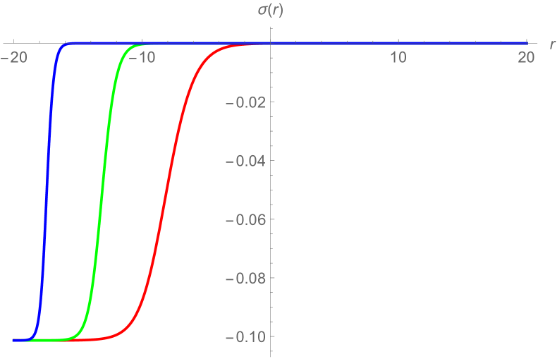
(a) Solutions for $\sigma(r)$

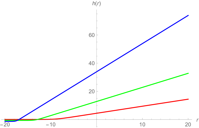
(b) Solutions for $h(r)$

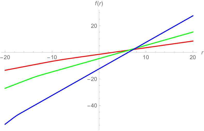
(c) Solutions for $f(r)$

Figure 1: Supersymmetric RG flows from $N=2$ SCFT in five dimensions to $N=2$ SCFT in three dimensions from $ISO(3)$ $F(4)$ gauged supergravity with $g=3m$ and $m=\frac{1}{4}$ (red), $m=\frac{1}{2}$ (green), $m=1$ (blue).

Similarly, we can find examples of numerical flow solutions interpolating between the $AdS_{6}$ vacuum and $AdS_{4}\times H^{2}$ geometry (44) as shown in figure 2. In these solutions, we have set $g=3m$, $m=\frac{1}{4}$ and $b=-1$ (red), $b=1$ (green), $b=2$ (blue). In this case, we have $\phi_{1}=\phi_{2}=0$ along the entire flows. As in the previous case, irrelevant operators are not turned on. In this case, near the $AdS_{6}$ critical point, we find

$$\sigma\sim e^{-\frac{3r}{L}}\qquad\textrm{and}\qquad\phi_{5}\sim e^{-\frac{3r}{L}},$$ (46)

so the flow solutions are driven by vacuum expectation values of two relevant operators of dimension $3$ dual to $\phi_{5}$ and $\sigma$.

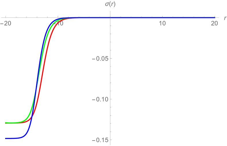
(a) Solutions for $\sigma(r)$

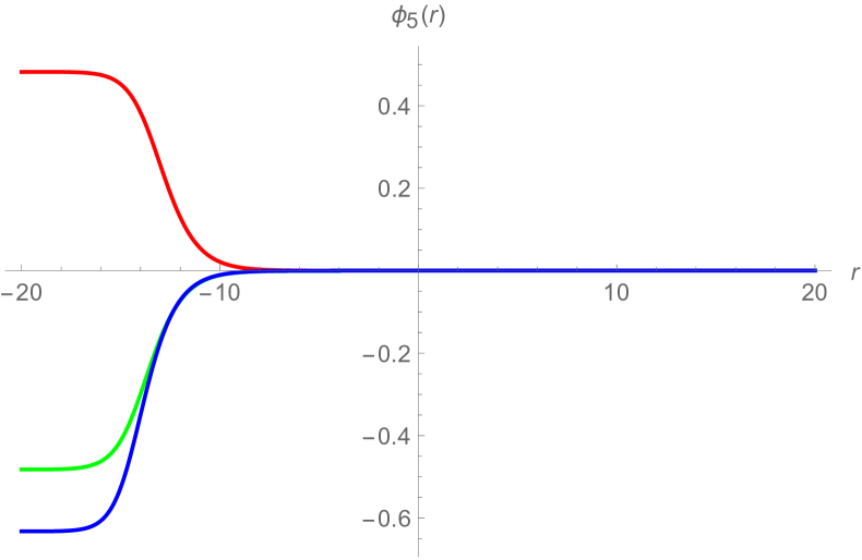
(b) Solutions for $\phi_{5}(r)$

(c) Solutions for $h(r)$

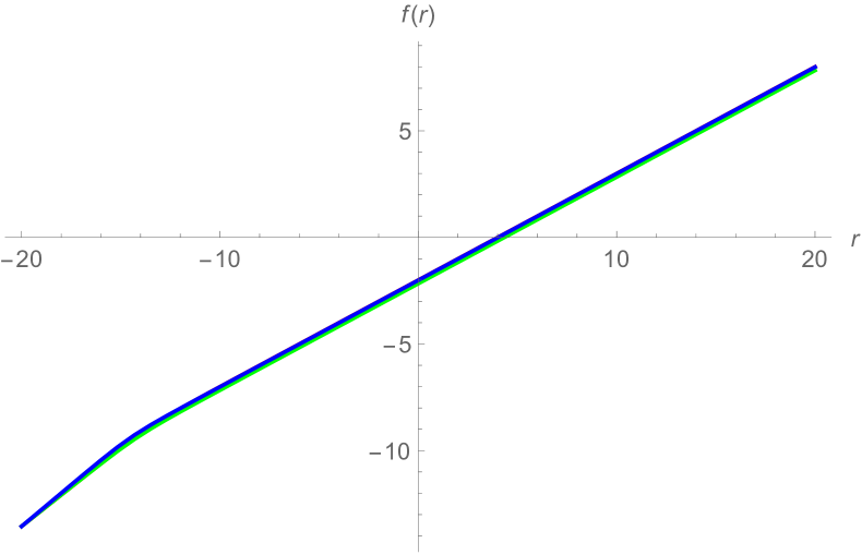
(d) Solutions for $f(r)$

Figure 2: Supersymmetric RG flows from $N=2$ SCFT in five dimensions to $N=2$ SCFT in three dimensions from $ISO(3)\times U(1)$ $F(4)$ gauged supergravity with $g=3m$, $m=\frac{1}{4}$ and $b=-1$ (red), $b=1$ (green), $b=2$ (blue).

3.2 Compactifications to two dimensions

In this section, we repeat a similar analysis for finding supersymmetric $AdS_{3}\times\mathcal{M}_{3}$ solutions to the $ISO(3)\times U(1)$ $F(4)$ gauged supergravity. We will work with a constant curvature manifold $\mathcal{M}_{3}$ described by the metric ansatz

$$ds^{2}=e^{2f(r)}dx^{2}_{1,1}+dr^{2}+e^{2h(r)}\left[d\psi^{2}+F_{\kappa}(\psi)^{2}(d\theta^{2}+\sin^{2}\theta d\phi^{2})\right]$$ (47)

with

$$F_{\kappa}(\psi)=\begin{cases}\sin\psi,&\kappa=1\phantom{-}\quad\textrm{for}\quad\mathcal{M}_{3}=S^{3}\\ \psi,&\kappa=0\phantom{-}\quad\textrm{for}\quad\mathcal{M}_{3}=T^{3}\\ \sinh\psi,&\kappa=-1\quad\textrm{for}\quad\mathcal{M}_{3}=H^{3}\end{cases}\,.$$ (48)

Using the following choice of vielbein

$$e^{\hat{a}}=e^{f}dx^{a},\qquad e^{\hat{r}}=dr,\qquad e^{\hat{\psi}}=e^{h}d\psi,$$

$$e^{\hat{\theta}}=e^{h}F_{\kappa}(\psi)d\theta,\qquad e^{\hat{\phi}}=e^{h}F_{\kappa}(\psi)\sin\theta d\phi,$$ (49)

with $a=0,1$, we find non-vanishing components of the spin connection of the form

$${\omega^{\hat{a}}}_{\hat{r}}=f^{\prime}e^{\hat{a}},\qquad{\omega^{\hat{\psi}}}_{\hat{r}}=h^{\prime}e^{\hat{\psi}},\qquad{\omega^{\hat{\theta}}}_{\hat{r}}=h^{\prime}e^{\hat{\theta}},\qquad{\omega^{\hat{\phi}}}_{\hat{r}}=h^{\prime}e^{\hat{\phi}},$$

$${\omega^{\hat{\phi}}}_{\hat{\psi}}=\frac{F^{\prime}_{\kappa}(\psi)}{F_{\kappa}(\psi)}e^{-h}e^{\hat{\phi}},\qquad{\omega^{\hat{\phi}}}_{\hat{\theta}}=\frac{e^{-h}}{F_{\kappa}(\psi)}\cot\theta e^{\hat{\phi}},\qquad{\omega^{\hat{\theta}}}_{\hat{\psi}}=\frac{F^{\prime}_{\kappa}(\psi)}{F_{\kappa}(\psi)}e^{-h}e^{\hat{\theta}}\,.\quad$$ (50)

We first note that the spin connection contains internal components on $\mathcal{M}_{3}$ only along $\theta$ and $\phi$ directions. To cancel these connections by performing a topological twist, we turn on the following $SO(3)\subset ISO(3)$ gauge fields

$$A^{1}=-a\cos\theta d\phi,\qquad A^{2}=-aF^{\prime}_{\kappa}(\psi)\sin\theta d\phi,\qquad A^{3}=-aF^{\prime}_{\kappa}(\psi)d\theta\,.$$ (51)

We recall that this $SO(3)$ subgroup is generated by $X_{r}$. There are two $SO(3)$ singlet scalars parametrized by the following coset representative, see more detail in [53],

$$L=e^{\phi\hat{Y}_{1}}e^{\varphi\hat{Y}_{2}}\,.$$ (52)

with

$$\hat{Y}_{1}=Y_{11}+Y_{22}+Y_{33}\qquad\textrm{and}\qquad\hat{Y}_{2}=Y_{04}\,.$$ (53)

This leads to the composite connection of the form

$$Q_{AB}=-\frac{i}{2}gA^{r}\sigma^{r}_{AB}\,.$$ (54)

The relevant terms in the gravitino variations are then given by

$$\delta\psi_{A\hat{\theta}}: \,0=\frac{1}{2}\frac{F^{\prime}_{\kappa}(\psi)}{F_{\kappa}(\psi)}e^{-h}\gamma_{\hat{\theta}\hat{\psi}}\epsilon_{A}-\frac{i}{2}gA^{r}_{\hat{\theta}}\sigma^{r}_{AB}\epsilon^{B}+\ldots,$$

$$\delta\psi_{A\hat{\phi}}: \,0=\frac{1}{2}\frac{F^{\prime}_{\kappa}(\psi)}{F_{\kappa}(\psi)}e^{-h}\gamma_{\hat{\phi}\hat{\psi}}\epsilon_{A}+\frac{1}{2}\frac{\cot\theta}{F_{\kappa}(\psi)}e^{-h}\gamma_{\hat{\phi}\hat{\theta}}\epsilon_{A}-\frac{i}{2}gA^{r}_{\hat{\phi}}\sigma^{r}_{AB}\epsilon^{B}+\ldots\quad\,.$$ (55)

The twist is achieved by imposing the twist condition

$$ag=1$$ (56)

and the following projectors

$$\gamma_{\hat{\theta}\hat{\psi}}=-i\sigma^{3}_{AB}\epsilon^{B},\qquad\gamma_{\hat{\phi}\hat{\psi}}=-i\sigma^{2}_{AB}\epsilon^{B},\qquad\gamma_{\hat{\phi}\hat{\theta}}=-i\sigma^{1}_{AB}\epsilon^{B}\,.$$ (57)

It should be noted that only two of these projectors are independent, so the $AdS_{3}\times\mathcal{M}_{3}$ solutions will preserve four supercharges. In the dual five-dimensional $N=2$ SCFT, the $16$ supercharges transform under $SO(1,4)\times SO(3)_{R}$ as $(\mathbf{4},\mathbf{2})$ and $(\bar{\mathbf{4}},\mathbf{2})$. Under the decomposition to two dimensions, we have $SO(1,4)\rightarrow SO(1,1)\times SO(3)$ under which $\mathbf{4}\rightarrow\mathbf{2}_{1}+\mathbf{2}_{-1}$. The original $16$ supercharges then transform under $SO(1,1)\times SO(3)\times SO(3)_{R}$ as

$$(\mathbf{4},\mathbf{2})+(\bar{\mathbf{4}},\mathbf{2})\rightarrow 2\times(\mathbf{2}_{1}+\mathbf{2}_{-1},\mathbf{2}).$$ (58)

After imposing the topological twist by identifying the $SO(3)$ with the $SO(3)_{R}$ symmetry, we end up with the following decomposition

$$(\mathbf{4},\mathbf{2})+(\bar{\mathbf{4}},\mathbf{2})\rightarrow 2\times(\mathbf{1}_{1}+\mathbf{1}_{-1}+\mathbf{3}+\mathbf{3})$$ (59)

under $SO(1,1)\times SO(3)_{\textrm{diag}}$. The unbroken supersymmetry is then generated by the singlet supercharges and corresponds to $N=(1,1)$ superconformal symmetry in two dimensions, see also the discussion in [29].
In order to derive the BPS equations, it is useful to note the explicit form of the gauge field strength tensors

$$F^{1}_{\hat{\theta}\hat{\phi}}=\frac{1}{2}\kappa ae^{-2h},\qquad F^{2}_{\hat{\psi}\hat{\phi}}=\frac{1}{2}\kappa ae^{-2h},\qquad F^{3}_{\hat{\psi}\hat{\theta}}=\frac{1}{2}\kappa ae^{-2h}\,.$$ (60)

As in the previous case, with the ansatz for the gauge fields given above, it is consistent to set the two-form field to zero. With all these, we find the following BPS equations

$$\phi^{\prime} = \frac{1}{4}e^{-2h-\sigma-\phi}(e^{2\phi}-1)(4ge^{2h+2\sigma+2\phi}-\kappa a),$$ (61)

$$\varphi^{\prime} = -2me^{-3\sigma}\sinh\varphi,$$ (62)

$$\sigma^{\prime} = \frac{1}{4}e^{-3\sigma-\varphi}\left[ge^{4\sigma+\phi+\varphi}(e^{2\phi}-3)+3m(1+e^{2\varphi})\right]+\frac{3}{8}\kappa ae^{-2h-\sigma}\cosh\phi,$$ (63)

$$h^{\prime} = \frac{1}{4}e^{-3\sigma}\left[ge^{4\sigma+\phi}(3-e^{2\phi})+m(e^{\varphi}+e^{-\varphi})\right]+\frac{5}{8}\kappa ae^{-2h-\sigma}\cosh\phi,$$ (64)

$$f^{\prime} = \frac{1}{4}e^{-3\sigma}\left[ge^{4\sigma+\phi}(3-e^{2\phi})+m(e^{\varphi}+e^{-\varphi})\right]-\frac{3}{8}\kappa ae^{-2h-\sigma}\cosh\phi\,.$$ (65)

It can also be checked that all these equations satisfy the field equations. It turns out that these equations admit only one $AdS_{3}\times\mathcal{M}_{3}$ fixed point given by

$$\phi=\varphi=0,\qquad\sigma=\frac{1}{4}\ln\left[\frac{3m}{2g}\right],$$

$$h=\frac{1}{2}\ln\left[-\sqrt{\frac{3}{2}}\frac{\kappa a}{\sqrt{gm}}\right],\qquad\frac{1}{L_{AdS_{3}}}=2\left(\frac{2}{3}\right)^{\frac{3}{4}}m^{\frac{1}{4}}g^{\frac{3}{4}}\,.$$ (66)

As in the previous case, the fixed point exists only for $\kappa=-1$ giving rise to an $AdS_{3}\times H^{3}$ solution. Examples of numerical solutions interpolating between this geometry and the $AdS_{6}$ vacuum are given in figure 3 for $g=3m$ and $m=\frac{1}{4}$ (red), $m=\frac{1}{2}$ (green), $m=1$ (blue). Since $\varphi=0$ both at the $AdS_{3}\times H^{3}$ fixed point and along the flow, the solutions can also be regarded as solutions of $ISO(3)$ $F(4)$ gauged supergravity coupled to three vector multiplets. The solutions describe RG flows from the five-dimensional $N=2$ SCFT to a two-dimensional $N=(1,1)$ SCFT in the IR. Equivalently, the solutions can also be interpreted as supersymmetric black strings in asymptotically $AdS_{6}$ space.
As in the previous case, $\sigma$ participates in the flows with the behavior near the $AdS_{6}$ vacuum

$$\sigma\sim e^{-\frac{3r}{L}}\,.$$ (67)

This again implies that the flow is driven by a vacuum expectation value of a dimension-$3$ operator.

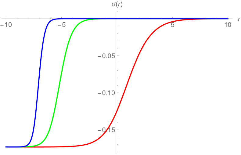
(a) Solutions for $\sigma(r)$

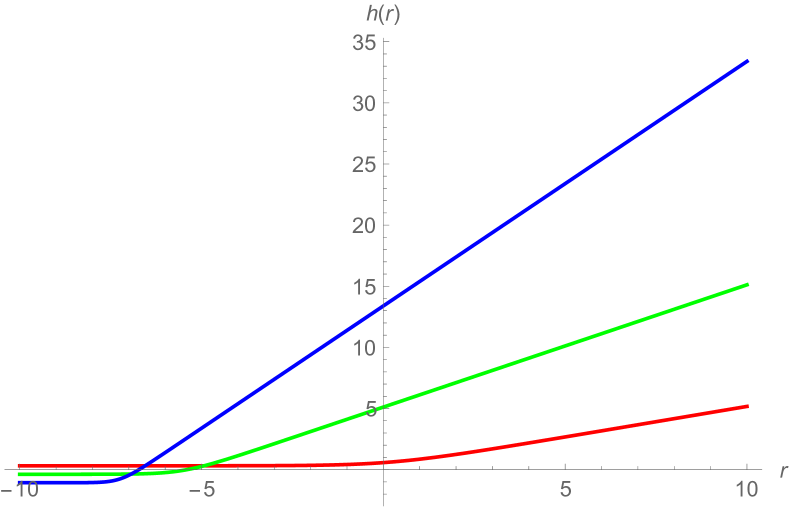
(b) Solutions for $h(r)$

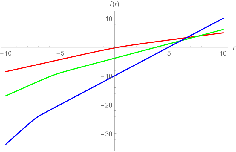
(c) Solutions for $f(r)$

Figure 3: Supersymmetric RG flows from $N=2$ SCFT in five dimensions to $N=(1,1)$ SCFT in two dimensions from $ISO(3)$ $F(4)$ gauged supergravity.

4 Line and surface defects from ISO(3)$\times$U(1) $F(4)$ gauged supergravity

In this section, we consider another class of holographic solutions describing conformal line and surface defects within the $N=2$ SCFT in five dimensions. These solutions break five-dimensional superconformal symmetry but preserve conformal symmetries in one and two dimensions. The supergravity solutions realizing these defects take the form of curved domain walls with $AdS_{2}\times S^{3}$ and $AdS_{3}\times S^{2}$ slices, respectively. These curved domain walls are supported by a non-vanishing two-form field from the supergravity multiplet. For simplicity, we will truncate out all the vector fields. Therefore, the solutions we will consider only involve the metric, scalars and the two-form field.

4.1 Line defects

We first consider solutions that are holographically dual to conformal line defects within the $N=2$ SCFT in five dimensions. The metric ansatz takes the form

$$ds^{2}=e^{2f(r)}ds^{2}_{AdS_{2}}+dr^{2}+e^{2h(r)}ds^{2}_{S^{3}}\,.$$ (68)

We will accordingly split the six-dimensional coordinates as $x^{\mu}=(x^{a},r,\theta^{i})$ for $a=0,1$ and $i=1,2,3$. As in [37] and [46], we will take the ansatz for the two-form field to be

$$B=b(r)\textrm{vol}_{AdS_{2}}\,.$$ (69)

As pointed out in [38], with vanishing gauge fields, the action of supersymmetry transformations on $SU(2)_{R}$ indices $A,B$ is trivial. The two chiralities of the Symplectic-Majorana-Weyl spinors can then be conveniently combined into a Dirac spinor. The Killing spinors for the solutions of interest take the form

$$\epsilon=\epsilon^{+}+\epsilon^{-}$$ (70)

with

$$\epsilon^{+}=iY(r)\left[\cos\theta(r)\chi^{+}\otimes\epsilon_{0}+\sin\theta(r)\chi^{+}\otimes\sigma_{3}\epsilon_{0}\right]\otimes\eta,$$

$$\epsilon^{-}=Y(r)\left[\sin\theta(r)\chi^{-}\otimes\epsilon_{0}-\cos\theta(r)\chi^{-}\otimes\sigma_{3}\epsilon_{0}\right]\otimes\eta\,.$$ (71)

In this equation, $\epsilon_{0}$ is a two-component constant spinor while $\chi^{\pm}$ and $\eta$ are respectively Killing spinors on $AdS_{2}$ and $S^{3}$ satisfying

$$\hat{\nabla}_{a}\chi^{\pm}=\pm\frac{i}{2\ell}\rho_{a}\chi^{\mp}\qquad\textrm{and}\qquad\widetilde{\nabla}_{i}\eta=\frac{i}{2R}\tilde{\gamma}_{i}\eta\,.$$ (72)

$\ell$ and $R$ denote the radii of $AdS_{2}$ and $S^{3}$, respectively.
As in [46], we use the following form of gamma matrices

$$\gamma^{a}=\rho^{a}\otimes\sigma_{2}\otimes\mathbb{I}_{2},\qquad\gamma^{r}=\rho_{*}\otimes\sigma_{2}\otimes\mathbb{I}_{2},$$

$$\gamma^{i}=-\mathbb{I}_{2}\otimes\sigma_{1}\otimes\tilde{\gamma}^{i},\qquad\gamma_{7}=-i\mathbb{I}_{2}\otimes\sigma_{3}\otimes\mathbb{I}_{2}\,.$$ (73)

In these equations, the chirality matrix on $AdS_{2}$ is defined by $\rho_{*}=\rho^{0}\rho^{1}$ with $\rho^{2}_{*}=\mathbb{I}_{2}$.
We now analyze the BPS conditions arising from setting supersymmetry transformations of fermions to zero. The coset representative is taken to be the $SO(2)\times U(1)$ symmetric one given in (27). Since we have set all the gauge fields to zero, we need to set $\phi_{3}=0$. Due to various similarities between the forms of relevant equations in this case and those of compact $SU(2)\times SU(2)$ gauge group considered [46], the analysis is essentially the same as in [46] to which we refer for more detail. We first need to impose a projection condition on the Killing spinors

$$\sigma_{2}\epsilon_{0}=\epsilon_{0}\,.$$ (74)

We also note that this is related to a $\gamma_{r}$ projector. We now consider the gaugino variations $\delta\lambda^{I}_{A}$. Since the two-form field does not appear in these variations, we simply obtain the following equations from $\delta\lambda^{1,2}_{A}$

$$\left[\phi^{\prime}_{1}+M_{1}+iM_{2}\right]\cos\theta = 0,$$

$$\left[\phi^{\prime}_{1}-M_{1}-iM_{2}\right]\sin\theta = 0$$ (75)

with

$$M_{1}=2ge^{\sigma+2\phi_{1}}(\cosh\phi_{0}\cosh\phi_{5}\sinh\phi_{2}+\sinh\phi_{0}\sinh\phi_{4}\sinh\phi_{5}),$$

$$M_{2}=-2ge^{\sigma+2\phi_{1}}\sinh\phi_{0}\cosh\phi_{4}\,.$$ (76)

For convenience, we also point out that the two equations in (75) arise from setting the coefficients of $(\chi^{+}\otimes\epsilon_{0}\otimes\eta,\chi^{-}\otimes\sigma_{3}\epsilon_{0}\otimes\eta)$ and $(\chi^{+}\otimes\sigma_{3}\epsilon_{0}\otimes\eta,\chi^{-}\otimes\epsilon_{0}\otimes\eta)$ to zero, respectively.
Consistency of these two equations implies $M_{2}=0$ which leads to

$$\phi_{0}=0\,.$$ (77)

Furthermore, to obtain non-trivial BPS equations for scalar fields, we have to set either $\sin\theta=0$ or $\cos\theta=0$ leading to the following BPS equations

$$\phi_{1}^{\prime}=\mp M_{1}\,.$$ (78)

This is exactly the same structure found in [46] for compact gauging of the matter-coupled $F(4)$ gauged supergravity.
Similarly, $\delta\lambda^{3}_{A}$ and $\delta\lambda^{4}_{A}$ give

$$\cosh\phi_{5}\phi^{\prime}_{2} = \pm M_{3},$$

$$\cosh\phi_{5}\phi^{\prime}_{4} = \pm\widetilde{M}_{0},$$

$$\phi_{5}^{\prime} = \mp\widetilde{M}_{3}$$ (79)

with

$$M_{3}=2ge^{\sigma}\left[(e^{2\phi_{1}}-1)\cosh\phi_{2}-\sinh\phi_{2}\right],$$

$$\widetilde{M}_{0}=2me^{-3\sigma}\cosh\phi_{5}\sinh\phi_{4},$$

$$\widetilde{M}_{3}=-2ge^{\sigma}\cosh\phi_{5}\sinh\phi_{5}+4ge^{\sigma+\phi_{1}}\sinh\phi_{1}\sinh\phi_{2}\sinh\phi_{5}\,.$$ (80)

In the three equations in (79), we have also used $\phi_{0}=0$ and $\sin\theta=0$ or $\cos\theta=0$.
Consistency of the BPS equations from $\delta\chi_{A}$ and $\delta\psi_{A\mu}$ leads to another condition of the form

$$\sinh\phi_{4}\sinh\phi_{5}=0$$ (81)

which further implies that we can have solutions with either $\phi_{4}=0$ or $\phi_{5}=0$. However, it turns out that the two-form field equation requires $\phi_{4}=0$. Taking into account all of these results, we eventually arrive at the following set of the BPS equations

$$\phi^{\prime}_{1} = 2ge^{\sigma+2\phi_{1}}\cosh\phi_{5}\sinh\phi_{2},$$ (82)

$$\phi^{\prime}_{2} = 2ge^{\sigma}\textrm{sech}\phi_{5}\left[(e^{2\phi_{1}}-1)\cosh\phi_{2}-\sinh\phi_{2}\right],$$ (83)

$$\phi_{5}^{\prime} = -2ge^{\sigma}\sinh\phi_{5}\left(\cosh\phi_{2}-2e^{\phi_{1}}\sinh\phi_{1}\sinh\phi_{2}\right),$$ (84)

$$\sigma^{\prime} = \frac{1}{2}ge^{\sigma}\cosh\phi_{2}\cosh\phi_{5}-\frac{3}{2}me^{-3\sigma}-ge^{\sigma+\phi_{1}}\cosh\phi_{5}\sinh\phi_{1}\sinh\phi_{2},$$ (85)

$$b^{\prime} = 2me^{-3\sigma}b,$$ (86)

$$f^{\prime} = ge^{\sigma+\phi_{1}}\cosh\phi_{5}\sinh\phi_{1}\sinh\phi_{2}-\frac{1}{2}me^{-3\sigma}-\frac{1}{2}ge^{\sigma}\cosh\phi_{2}\cosh\phi_{5},$$ (87)

$$Y^{\prime} = \frac{1}{2}Yf^{\prime},\qquad h^{\prime}=f^{\prime}$$ (88)

together with two algebraic constraints

$$b=-\frac{e^{f+\sigma}}{\ell m}\qquad\textrm{and}\qquad R=\frac{2\ell e^{2f-h+\sigma}}{2e^{f+\sigma}-\ell mb}\,.$$ (89)

It is useful to point out that these two constraints result from the fact that $\delta\chi_{A}$, $\delta\psi_{Aa}$ and $\delta\psi_{Ai}$ lead to three different BPS equations for $b(r)$. Taking one of them as a flow equation for $b(r)$ and requiring this equation be equivalent to the remaining two equations give rise to the aforementioned two algebraic constraints, see more detail in [46]. In the BPS equations, we have also chosen a particular sign choice to identify the $AdS_{6}$ vacuum as $r\rightarrow\infty$.
Since the BPS equations for $h^{\prime}$ and $f^{\prime}$ are the same, we imediately find that $f=h+C$ for a constant $C$. The constant $C$ can be chosen to be zero by requiring that the solution becomes locally $AdS_{6}$ geometry with $f\sim h\sim\frac{r}{L}$. Therefore, we will set $f(r)=h(r)$ from now on. We have also verified that the BPS equations are compatible with the two algebraic constraints and the corresponding second-ordered field equations. We are not able to analytically solve these equations in full generality. This requires some numerical analysis which can always be achived by suitable boundary conditions. We will instead consider some interesting solutions that can be obtained analytically within particular subtruncations. These solutions could be much more useful in most proposes.
We first consider a subtruncation with $\phi_{1}=\phi_{2}=0$. This effectively turns off irrelevant operators dual to $\phi_{1}$ and $\phi_{2}$ at the $AdS_{6}$ vacuum. With a simpler set of equations, we can now solve for the following solution

$$\phi_{5} = \ln\left[\frac{1+e^{-2g(\rho-\rho_{0})}}{1-e^{-2g(\rho-\rho_{0})}}\right],$$

$$\sigma = \frac{1}{4}\ln\left[\frac{\sinh\phi_{5}(\sigma_{0}+3m\coth\phi_{5})}{g}\right],$$

$$f = \frac{1}{12}\ln(3m\cosh\phi_{5}+\sigma_{0}\sinh\phi_{5})-\frac{1}{3}\ln\sinh\phi_{5},$$

$$b = -\frac{(\sigma_{0}+3m\coth\phi_{5})^{\frac{1}{3}}}{\ell mg^{\frac{1}{4}}},\qquad Y=e^{\frac{f}{2}}$$ (90)

with $\sigma_{0}$ being an integration constant and $\rho$ defined by $\frac{d\rho}{dr}=e^{\sigma}$. First of all, we notice that the solution approaches the $AdS_{6}$ vacuum with $\phi_{5}=0$ and $\sigma=\frac{1}{4}\ln\left[\frac{3m}{g}\right]$ for any value of $\sigma_{0}$. This solution takes the same form as the holographic RG flow studied in [53] with a non-vanishing two-form field. This type of solutions is called charged domain walls in [37] and [38]. Near the $AdS_{6}$ vacuum, we find

$$\phi_{5}\sim\sigma\sim e^{-\frac{3r}{L}}\qquad\textrm{and}\qquad b\sim\phi_{5}^{-\frac{1}{3}}\sim e^{\frac{r}{L}}$$ (91)

in which we have set $g=3m$. From this behavior, we see that $\phi_{5}$ and $\sigma$ correspond to vacuum expectation values of relevant operators of dimension $3$ while $b$ is dual to a dimension-$4$ operator as in the solutions considered in [39, 46]. The asymptotic behavior also indicates that the line defect involves a source of this dimension-$4$ operator. The solution is singular at $\rho=\rho_{0}$ with

$$\phi_{5}\sim-\ln(\rho-\rho_{0})$$ (92)

and

$$\sigma\sim\frac{1}{4}\ln(\rho-\rho_{0}),\qquad f\sim\frac{5}{12}\ln(\rho-\rho_{0}),\qquad b\sim-\frac{6^{\frac{1}{3}}(\rho-\rho_{0})^{\frac{2}{3}}}{\ell g^{\frac{1}{4}}m^{\frac{2}{3}}}$$ (93)

for $\sigma_{0}=-3m$, and

$$\sigma\sim-\frac{1}{4}\ln(\rho-\rho_{0}),\qquad f\sim\frac{1}{4}\ln(\rho-\rho_{0}),\qquad b\sim-\frac{(3m+\sigma_{0})^{\frac{1}{3}}}{\ell g^{\frac{1}{4}}m}$$ (94)

for $\sigma_{0}\neq-3m$. These are the same asymptotic behaviors of scalars studied in [53] in the case of holographic RG flows to non-conformal phases of the $N=2$ SCFT.
Another solution we will consider is given by $\phi_{5}=0$ and $\phi_{2}=\phi_{1}$. Unlike the previous solution with $SO(2)\times U(1)$ symmetry, this solution preserves a larger $SO(3)\times U(1)$ symmetry and is given by

$$g(\rho-\rho_{0}) = e^{-\phi_{1}}+\frac{1}{2}\ln\left[\frac{1-e^{-\phi_{1}}}{1+e^{-\phi_{1}}}\right],$$

$$\sigma = \frac{1}{4}\ln\left[\frac{e^{-\phi_{1}}(\tilde{\sigma}_{0}e^{4\phi_{1}}-3m)}{2g(e^{2\phi_{1}}-1)}\right],$$

$$f = \frac{1}{4}\ln(1-e^{2\phi_{1}})+\frac{1}{12}\ln(3m-\tilde{\sigma}_{0}e^{4\phi_{1}})-\frac{13}{12}\phi_{1},$$

$$b = -\frac{e^{-\frac{4}{3}\phi_{1}}(3m-\tilde{\sigma}_{0}e^{4\phi_{1}})^{\frac{1}{3}}}{\ell m(2g)^{\frac{1}{4}}},\qquad Y=e^{\frac{f}{2}}$$ (95)

with the same coordinate $\rho$ as in the previous case and another integration constant $\tilde{\sigma}_{0}$. This solution also takes the form of a charged domain wall. In this case, however, we need to set $\tilde{\sigma}_{0}=3m$ in order to obtain the asymptotically $AdS_{6}$ geometry as $r\rightarrow\infty$. Near the $AdS_{6}$ vacuum, we find

$$\phi_{1}\sim e^{\frac{3r}{L}},\qquad\sigma\sim\phi_{1}^{-1}\sim e^{-\frac{3r}{L}},\qquad b\sim\phi_{1}^{\frac{1}{3}}\sim e^{\frac{r}{L}}\,.$$ (96)

As in the previous case, there is a source for an operator of dimension $4$ dual to the two form field $b$. The dilaton $\sigma$ and $\phi_{1}$ correspond to a vacuum expectation value of a dimension-$3$ operator as before and a source of a dimension-$8$ operator, respectively. As $\rho\rightarrow\rho_{0}$, we find, see more detail in [53],

$$\phi_{1}\sim-\frac{1}{3}\ln(\rho-\rho_{0}),\qquad\sigma\sim-\frac{1}{12}\ln(\rho-\rho_{0}),$$

$$f\sim\frac{1}{12}\ln(\rho-\rho_{0}),\qquad b\sim-\frac{3^{\frac{1}{3}}}{(2g)^{\frac{1}{4}}m^{\frac{2}{3}}\ell}\,.$$ (97)

This behavior is again the same as the RG flow solution considered in [53] with a non-vanishing two-form field.

4.2 Surface defects

We now repeat a similar analysis for solutions describing conformal surface defects within the $N=2$ SCFT in five dimensions. The metric ansatz is now given by

$$ds^{2}=e^{2f(r)}dx^{2}_{AdS_{3}}+dr^{2}+e^{2h(r)}ds^{2}_{S^{2}}\,.$$ (98)

The solutions preserve two-dimensional conformal symmetry corresponding to the $AdS_{3}$ factor. Similar to the previous analysis, we will also turn on the two-form field with the ansatz

$$B=b(r)\textrm{vol}_{S^{2}}\,.$$ (99)

The scalar fields are given by the coset representative in (27).
In this case, we will split the six-dimensional coordinates as $x^{\mu}=(x^{a},r,\theta^{i})$ with $a=0,1,2$ and $i=1,2$ and take the Killing spinors to be

$$\epsilon=Y\eta\otimes\left[\cos\theta\chi^{+}\otimes\epsilon_{0}+i\sin\theta\gamma_{*}\chi^{+}\otimes\sigma_{3}\epsilon_{0}-i\cos\theta\gamma_{*}\chi^{-}\otimes\sigma_{3}\epsilon_{0}+\sin\theta\chi^{-}\epsilon_{0}\right].$$ (100)

The Killing spinors on $AdS_{3}$ and $S^{2}$, denoted by $\eta$ and $\chi^{\pm}$, respectively satisfy

$$\hat{\nabla}_{a}=\frac{1}{2\ell}\rho_{a}\eta\qquad\textrm{and}\qquad\tilde{\nabla}_{i}\chi^{\pm}=\frac{1}{2R}\gamma_{*}\tilde{\gamma}_{i}\chi^{\mp}\,.$$ (101)

In this case, $\ell$ and $R$ are respectively $AdS_{3}$ and $S^{2}$ radii. The gamma matrices are chosen to be

$$\gamma^{a}=\rho^{a}\otimes\mathbb{I}_{2}\otimes\sigma,\qquad\gamma^{r}=-(\mathbb{I}_{2}\otimes\gamma_{*}\otimes\sigma_{1}),$$

$$\gamma^{i}=-(\mathbb{I}_{2}\otimes\tilde{\gamma}^{i}\otimes\sigma_{1}),\qquad\gamma_{7}=i\mathbb{I}_{2}\otimes\mathbb{I}_{2}\otimes\sigma_{3}$$ (102)

with $\gamma_{*}=i\tilde{\gamma}^{1}\tilde{\gamma}^{2}$ and $\gamma_{*}^{2}=\mathbb{I}_{2}$.
To derive the BPS equations, we impose the following projector on the Killing spinors

$$(\gamma_{*}\otimes\sigma_{1})(\chi^{\pm}\otimes\epsilon_{0})=\pm\chi^{\pm}\otimes\epsilon_{0}\,.$$ (103)

It is also useful to note that this projector implies

$$\chi^{\pm}\otimes\sigma_{2}\epsilon_{0}=\mp i\gamma_{*}\chi^{\pm}\otimes\sigma_{3}\epsilon_{0}\,.$$ (104)

The same analysis as in the case of line defects shows that the gaugino variations restrict the phase of the Killing spinors to satisfy $\sin\theta=0$ or $\cos\theta=0$. Consistency among the BPS equations again imposes the conditions $\phi_{0}=\phi_{4}=0$ in addition to $\phi_{3}=0$ required by a consistent truncation of gauge fields.
With all these and an appropriate sign choice to identify the $AdS_{6}$ vacuum with $r\rightarrow\infty$, we end up with the following set of BPS equations

$$\phi^{\prime}_{1} = 2ge^{\sigma+2\phi_{1}}\cosh\phi_{5}\sinh\phi_{2},$$ (105)

$$\phi_{2}^{\prime} = 2ge^{\sigma}\textrm{sech}\phi_{5}\left[(e^{2\phi_{1}}-1)\cosh\phi_{2}-\sinh\phi_{2}\right],$$ (106)

$$\phi_{5}^{\prime} = -2ge^{\sigma}\sinh\phi_{5}(\cosh\phi_{2}-2e^{\phi_{1}}\sinh\phi_{1}\sinh\phi_{2}),$$ (107)

$$\sigma^{\prime} = \frac{3}{2}me^{-3\sigma}-\frac{1}{2}g\cosh\phi_{5}(\cosh\phi_{2}-2e^{\phi_{1}}\sinh\phi_{1}\sinh\phi_{2}),$$ (108)

$$f^{\prime} = \frac{1}{2}ge^{\sigma}\cosh\phi_{5}(\cosh\phi_{2}-2e^{\phi_{1}}\sinh\phi_{1}\sinh\phi_{2})+\frac{1}{2}me^{-3\sigma},$$ (109)

$$Y^{\prime} = \frac{1}{2}Yf^{\prime},\qquad h^{\prime}=f^{\prime},$$ (110)

$$b^{\prime} = 2me^{-3\sigma}b$$ (111)

together with two algebraic constraints

$$b=-\frac{2e^{2h-f+\sigma}}{\ell m}\qquad\textrm{and}\qquad R=\frac{2\ell e^{f+h+\sigma}}{2e^{2h+\sigma}-\ell mbe^{f}}\,.$$ (112)

As in the case of line defects, we will consider two types of solutions that can be analytically obtained in particular subtruncations. The first type of solutions is found by setting $\phi_{2}=\phi_{1}=0$ which leads to the following solution

$$\phi_{5} = \ln\left[\frac{1+e^{-2g(\rho-\rho_{0})}}{1-e^{-2g(\rho-\rho_{0})}}\right],$$

$$\sigma = \frac{1}{4}\ln\left[\frac{\sinh\phi_{5}(\sigma_{0}+3m\coth\phi_{5})}{g}\right],$$

$$f = \frac{1}{12}\ln(3m\cosh\phi_{5}+\sigma_{0}\sinh\phi_{5})-\frac{1}{3}\ln\sinh\phi_{5},$$

$$b = -\frac{2}{\ell mg^{\frac{1}{4}}}(\sigma_{0}+3m\coth\phi_{5})^{\frac{1}{3}},\qquad Y=e^{\frac{f}{2}}$$ (113)

where, as before, $\rho$ is defined by $\frac{d\rho}{dr}=e^{\sigma}$ and $h=f$.
Another type of solutions is obtained by setting $\phi_{5}=0$ and $\phi_{2}=\phi_{1}$ giving rise to the solution

$$g(\rho-\rho_{0}) = e^{-\phi_{1}}+\frac{1}{2}\ln\left[\frac{1-e^{-\phi_{1}}}{1+e^{-\phi_{1}}}\right],$$

$$\sigma = \frac{1}{4}\ln\left[\frac{e^{-\phi_{1}}(\tilde{\sigma}_{0}e^{4\phi_{1}}-3m)}{2g(e^{2\phi_{1}}-1)}\right],$$

$$f = \frac{1}{4}\ln(1-e^{2\phi_{1}})+\frac{1}{12}\ln(3m-\tilde{\sigma}_{0}e^{4\phi_{1}})-\frac{13}{12}\phi_{1},$$

$$b = -\frac{2^{\frac{3}{4}}e^{-\frac{4}{3}\phi_{1}}(3m-\tilde{\sigma}_{0}e^{4\phi_{1}})^{\frac{1}{3}}}{\ell mg^{\frac{1}{4}}},\qquad Y=e^{\frac{f}{2}}\,.$$ (114)

with the same coordinate $\rho$ as in the previous solution. The integration constant $\tilde{\sigma}_{0}$ needs to be chosen as $\tilde{\sigma}_{0}=3m$ in order for the solution to approach the $AdS_{6}$ vacuum. All of these solutions take the same form as the solutions for line defects considered above with the only difference being a numerical factor in the solution for $b$. Asymptotic behaviors are the same as in the case of line defects, and we will not repeat these again. We simply point out that the surface defects also arise from turning on a dimension-$4$ operator dual to the two-form field as in the case of line defects. Although the solutions in both cases take the same form, we expect that the two types of solutions lead to different uplifted ten-dimensional solutions. In particular, in the case of line defects, we have an electric component of the two-form field while the magnetic component appears in the case of surface defects.

5 Conclusions

We have studied a number of supersymmetric solutions from matter-coupled $F(4)$ gauged supergravity with $ISO(3)\times U(1)$ gauge group. The first class of these solutions takes the form of RG flows across dimensions and holographically describes twisted compactifications of the five-dimensional $N=2$ SCFT on $H^{2}$ and $H^{3}$ to three- and two-dimensional SCFTs in the IR. These solutions have been obtained by performing standard topological twists using $SO(2)\times U(1)$ and $SO(3)$ gauge fields. Since the $ISO(3)\times U(1)$ $F(4)$ gauged supergravity is a consistent truncation of type IIB theory on $S^{2}\times\Sigma$, the $AdS_{4}\times H^{2}$ and $AdS_{3}\times H^{3}$ solutions found in this paper lead to new supersymmetric $AdS_{4}\times H^{2}\times S^{2}\times\Sigma$ and $AdS_{3}\times H^{3}\times S^{2}\times\Sigma$ solutions in type IIB theory.
The second class of solutions obtained in this paper takes the form of “charged” curved domain walls with $AdS_{2}\times S^{3}$ and $AdS_{3}\times S^{2}$ slicing. These solutions have been found by turning on the two-form field in the gravity multiplet to support the curvature of the domain walls. The solutions have a holographic interpretation as conformal line and surface defects within the $N=2$ SCFT in five dimensions. These defects arise from a source term for a dimension-$4$ operator dual to the two-form field. The solutions also have a very similar structure as those found in compact gauge groups studied in [46]. In particular, the solutions are mainly holographic RG flows in the presence of a running two-form field.
Although the matter-coupled $ISO(3)\times U(1)$ $F(4)$ gauged supergravity considered here can be embedded in type IIB theory, the complete truncation ansatz has not been constructed to date. It would be interesting to work this out using the formalism of exceptional field theories and use the resulting truncation ansatz to uplift the solutions found in this paper to ten dimensions. This could lead to new $AdS_{4}\times H^{2}$ and $AdS_{3}\times H^{3}$ solutions in type IIB theory as mentioned above as well as possible brane configurations whose near horizon geometries given by these solutions. It would also be interesting to identify the dual $N=2$ SCFT in five dimensions together with field theory descriptions of conformal line and surface defects dual to the solutions found here in terms of position-dependent deformations.
Acknowledgement
This work is funded by National Research Council of Thailand (NRCT) and Chulalongkorn University under grant N42A650263.

References

- [1] N. Seiberg, “Five dimensional SUSY field theories, non-trivial fixed points and string dynamics”, Phys. Lett. B388 (1996) 753-760, arXiv: hep-th/9608111.
- [2] D. R. Morrison and N. Seiberg, “Extremal transitions and five-dimensional supersymmetric field theories”, Nucl. Phys. B483 (1997) 229, arXiv: hep-th/9609070.
- [3] K. Intriligator, D. R. Morrison and N. Seiberg, “Five dimensional supersymmetric gauge theories and degenerations of Calabi-Yau spaces”, Nucl. Phys. B497 (1997) 56, arXiv: hep-th/9702198.
- [4] W. Nahm, “Supersymmetries and their representations”, Nucl. Phys. B 135 (1978) 149-166.
- [5] J. M. Maldacena, “The large limit of superconformal field theories and supergravity”, Adv. Theor. Math. Phys. 2 (1998) 231-252, arXiv: hep-th/9711200.
- [6] S. S. Gubser, I. R. Klebanov and A. M. Polyakov, “”, Phys. Lett. B428 (1998) 105-114, arXiv: hep-th/9802.109.
- [7] E. Witten, “Anti De Sitter Space and holography”, Adv. Theor. Math. Phys. 2 (1998) 253-291, arXiv: 9802150.
- [8] S. Ferrara, A. Kehagias, H. Partouche, A. Zaffaroni, “AdS6 interpretation of 5d superconformal field theories”, Phys. Lett. B431 (1998) 57-62, arXiv: hep-th/9804006.
- [9] A. Brandhuber and Y. Oz, “The D4-D8 brane system and five dimensional fixed points”, Phys. Lett. B460 (1999) 307-312, arXiv: hep-th/9905148.
- [10] D. Bashkirov, “A comment on the enhancement of global symmetries in superconformal gauge theories in 5D”, arXiv: 1211.4886.
- [11] O. Bergman and D. Rodriguez-Gomez, “5d quivers and their AdS(6) duals” JHEP 07 (2012) 171, arXiv: 1206.3503.
- [12] O. Bergman and D. Rodriguez-Gomez, “Probing the Higgs branch of 5D fixed point theories with dual giant gravitons in AdS(6)”, JHEP 12 (2012) 047, arXiv: 1210.0589.
- [13] O. Bergman, D. Rodriguez-Gomez and G. Zafrir, “5D superconformal indices at large and holography”, JHEP 08 (2013) 081, arXiv: 1305.6870.
- [14] A. Passias, “A note on supersymmetric AdS6 solutions of massive type IIA supergravity”, JHEP 01 (2013) 113, arXiv: 1209.3267.
- [15] F. Apruzzi, M. Fazzi, A. Passias, D. Rosa, and A. Tomasiello, “ solutions of type II supergravity”, JHEP 11 (2014) 099, arXiv: 1406.0852.
- [16] H. Kim, N. Kim and M. Suh, “Supersymmetric solutions of type IIB supergravity”, Eur. Phys. J. C75 10 (2015) 484, arXiv: 1506.05480.
- [17] E. D’Hoker, M. Gutperle and C. F. Uhlemann, “Holographic duals for five-dimensional superconformal quantum field theories”, Phys. Rev. Lett. 118 (2017) 101601, arXiv: 1611.09411.
- [18] O. Bergman, D. Rodriguez-Gomez and C. F. Uhlemann, “Testing AdS6/CFT5 in Type IIB with stringy operators”, JHEP 08 (2018) 127, arXiv: 1806.07898.
- [19] M. Fluder and C. F. Uhlemann, “Precision Test of AdS6/CFT5 in Type IIB String Theory”, Phys. Rev. Lett. 121 (2018) 17, 171603, arXiv: 1806.08374.
- [20] F. Apruzzi, L. Lin and C. Mayrhofer, “Phases of 5d SCFTs from M-/F-theory on Non-Flat Fibrations”, JHEP 05 (2019) 187, arXiv: 1811.12400.
- [21] C. F. Uhlemann, “Exact results for 5d SCFTs of long quiver type”, JHEP 11 (2019) 072, arXiv: 1909.01369.
- [22] P. B. Genolini, M. Honda, H. Kim, D. Tong and C. Vafa, “Evidence for a Non-Supersymmetric 5d CFT from Deformations of 5d SYM”, JHEP 05 (2020) 058, arXiv: 2001.00023.
- [23] L. J. Romans, “The gauged supergravity in six-dimensions”, Nucl. Phys B269 (1986) 691.
- [24] R. D’ Auria, S. Ferrara and S. Vaula, “Matter coupled supergravity and the AdS6/CFT5 correspondence”, JHEP 10 (2000) 013, arXiv: hep-th/0006107.
- [25] L. Andrianopoli, R. D’ Auria and S. Vaula, “Matter coupled gauged supergravity Lagrangian”, JHEP 05 (2001) 065, arXiv: hep-th/0104155.
- [26] U. Gursoy, C. Nunez and M. Schvellinger, “RG flows from Spin(7), CY 4-fold and HK manifolds to AdS, Penrose limits and pp waves”, JHEP 06 (2002) 015, arXiv: hep-th/0203124.
- [27] P. Karndumri, “Holographic RG flows in six dimensional F(4) gauged supergravity”, JHEP 01 (2013) 134, Erratum-ibid. JHEP 06 (2015) 165, arXiv: 1210.8064.
- [28] P. Karndumri, “Gravity duals of 5D N=2 SYM from F(4) gauged supergravity”, Phys. Rev. D90 (2014) 086009, arXiv: 1403.1150.
- [29] C. Nunez, I. Y. Park, M. Schvellinger and T. A. Tran, “Supergravity duals of gauge theories from F(4) gauged supergravity in six dimensions”, JHEP 04 (2001) 025, arXiv: hep-th/0103080.
- [30] P. Karndumri, “Twisted compactification of 5D SCFTs to three and two dimensions from gauged supergravity”, JHEP 09 (2015) 034, arXiv: 1507.01515.
- [31] M. Gutperle, J. Kaidi and H. Raj, “Janus solutions in six-dimensional gauged supergravity”, JHEP 12 (2017) 018, arXiv: 1709.09204.
- [32] P. Karndumri, “Janus and RG-flow interfaces from matter-coupled gauged supergravity”, arXiv: 2405.17169.
- [33] M. Suh, “Supersymmetric black holes from gauged supergravity”, JHEP 01 (2019) 035, arXiv: 1809.03517.
- [34] S. M. Hosseini, K. Hristov, A. Passias, A. Zaffaroni, “6D attractors and black hole microstates”, JHEP 12 (2018) 001, arXiv: 1809.10685.
- [35] M. Suh, “Supersymmetric black holes from matter coupled gauged supergravity”, JHEP 02 (2019) 108, arXiv: 1810.00675.
- [36] P. Karndumri, “New supersymmetric black holes from matter-coupled gauged supergravity”, Eur. Phys. J. Plus 139 (2024) 858, arXiv: 2403.01746.
- [37] G. Dibitetto and N. Petri, “ solutions and their massive IIA origin”, JHEP 05 (2019) 107, arXiv: 1811.11572.
- [38] G. Dibitetto and N. Petri, “Surface defects in the brane system”, JHEP 01 (2019) 193, arXiv: 1807.07768.
- [39] K. Chen and M. Gutperle, “Holographic line defects in gauged supergravity”, Phys. Rev. D100 (2019) 126015, arXiv: 1909.11127.
- [40] C. F. Uhlemann, “Wilson loops in 5d long quiver gauge theories”, JHEP 09 (2020) 145, arXiv: 2006.01142.
- [41] M. Gutperle and C. F. Uhlemann, “Surface defects in holographic 5d SCFTs”, JHEP 04 (2021) 134, arXiv: 2012.14547.
- [42] L. Santilli and C. F. Uhlemann, “3d defects in 5d: RG flows and defect F-maximization”, JHEP 06 (2023) 136, arXiv: 2305.01004.
- [43] F. Faedo, Y. Lozano and N. Petri, “Searching for surface defect CFTs within AdS3”, JHEP 11 (2020) 052, arXiv: 2007.16167.
- [44] F. Faedo, Y. Lozano and N. Petri, “New AdS3 near-horizons in Type IIB”, JHEP 04 (2021) 028, arXiv: 2012.07148.
- [45] Y. Lozano, N. Petri and C. Risco, “AdS2 near-horizons, defects and string dualities”, Phys. Rev. D107 (2023) 106012, arXiv: 2212.11095.
- [46] P. Karndumri, “Line and surface defects in 5D SCFT from matter-coupled gauged supergravity”, arXiv: 2406.18946.
- [47] J. M. Maldacena and C. Nunez, “Supergravity description of field theories on curved manifolds and a no go theorem”, Int. J. Mod. Phys. A16 (2001) 822-855, arXiv: hep-th/0007018.
- [48] L. J. Romans, “The gauged supergravity in six-dimensions”, Nucl. Phys B269 (1986) 691.
- [49] R. D’ Auria, S. Ferrara and S. Vaula, “Matter coupled supergravity and the AdS6/CFT5 correspondence”, JHEP 10 (2000) 013, arXiv: hep-th/0006107.
- [50] L. Andrianopoli, R. D’ Auria and S. Vaula, “Matter coupled gauged supergravity Lagrangian”, JHEP 05 (2001) 065, arXiv: hep-th/0104155.
- [51] M. Cvetic, H. Lu and C. N. Pope, “Gauged six-dimensional supergravity from massive type IIA”, Phys. Rev. Lett. 83 (1999) 5226, arXiv: hep-th/9906221.
- [52] E. Malek, H. Samtleben and V. V. Camell, “Supersymmetric and vacua and their consistent truncations with vector multiplets”, JHEP 04 (2019) 088, arXiv: 1901.11039.
- [53] P. Karndumri, “Holographic RG flows and Janus interfaces from ISO(3)U(1) gauged supergravity”, arXiv: 2409.20151.