The Revival of : A Natural Solution for with a Sub-GeV Dark Matter
Abstract
The experiments searching for a hidden gauge sector with a leptophilic neutral gauge boson have already ruled out as a feasible extension of the Standard Model (SM) gauge group () for explaining the observed discrepancy in . The paper proposes a simple extension of the minimal particle content of with a TeV-scale scalar leptoquark . Due to the non-trivial transformation of under , the model generates additional one-loop contributions to , reviving the considered gauge extension within the experimentally allowed regions of the parameter space. The model can also accommodate a viable Dark Matter (DM) candidate — a vector-like SM-singlet fermion in the sub-GeV mass regime. The theory provides a natural framework to test the proposed DM phenomenology through electron excitation signals. Moreover, the DM-specific observables and being connected through the New Physics (NP) parameters, the future beam dump experiments hunting for light, feebly interacting particles and the DM direct detection experiments are complementary to each other for constraining/falsifying the model.
I Introduction
The Standard Model has been tested to an exceptional degree of precision at the high-energy colliders and through various other experiments, establishing itself as the nature’s theory for strong and electroweak (EW) interactions. The recent examples include the discovery of 125 GeV Higgs boson at the Large Hadron Collider (LHC) ATLAS:2012yve ; CMS:2012qbp , and the remeasurement of the W-boson mass at the ATLAS ATLAS:2024erm and CMS CMS-PAS-SMP-23-002 , where SM predictions closely match with the experimental data. However, despite all its excellence as a theoretical framework, SM falls short to explain certain observations, e.g., the astrophysical and cosmological signatures of dark matter 1932BAN…..6..249O ; Zwicky:1933gu ; Zwicky:1937zza ; Metcalf:2003sz ; Planck:2018vyg , the discrepancy between the observed and predicted values of the anomalous magnetic moments of muon Muong-2:2023cdq and electron Parker_2018 ; Morel:2020dww , neutrino oscillations Pontecorvo:1967fh , etc. In the SM, particularly, the anomalous magnetic moment of muon has been predicted with a significant precision, including the EW and hadronic contributions Aoyama:2020ynm , while experiments have also measured it very precisely. Thus, is a crucial parameter to test the precision of the SM at the quantum level. However, the observations indicate a non-negligible difference between the experimentally measured and predicted values of Muong-2:2023cdq . Though a similar discrepancy has been observed for the electrons, measurements using the recoil on Cs Parker_2018 and Rb Morel:2020dww atoms result in a relative sign between the reported values. Definitely, such observations strengthen the possibility of having a theory beyond the standard model (BSM). However, the NP can only exist either at a higher energy scale or has to be weakly/selectively coupled to the SM fields to be consistent with the current experimental results. From the theoretical perspective, a quite natural and well-motivated way to construct a BSM framework is to extend the SM gauge group with an additional symmetry Langacker:2008yv . After spontaneous symmetry breaking (SSB), the NP interactions may arise through the associated neutral gauge boson , creating a room for various BSM observables that can’t be accommodated within the parameter space of the SM. Such abelian extensions of the SM can originate from Grand Unified Theories (GUT) Robinett:1982tq ; Langacker:1984dc , extra-dimensional models Antoniadis:1990ew ; Appelquist:2000nn or string compactifications Goodsell:2010ie . However, augmentations of can also be formulated from the accidental global symmetries of the SM. Classically, the SM Lagrangian features the global symmetry group , ensuring the conservation of baryon number and the individual lepton numbers []. The difference between any two lepton numbers, i.e., [ with ] can naturally be promoted to a gauge quantum number as the associated abelian group represents an anomaly-free theory even in its minimal form Foot:1990mn ; He:1991qd ; Foot:1994vd . These theories, with as the only NP field, provide a simple and direct explanation for the observed discrepancies in lepton — and being specific to and , respectively, whereas is a good theory for both of the discrepancies. Note that, the neutral gauge bosons of groups are automatically leptophilic with only loop-induced couplings to the quark sector, making them tough to constrain through the hadronic colliders. However, the parameter spaces can be deeply probed through other experiments Riordan:1987aw ; Bjorken:1988as ; Davier:1989wz ; Bross:1989mp ; Bjorken:2009mm ; Andreas:2012mt ; APEX:2011dww ; A1:2011yso ; NA64:2016oww ; CHARM:1985nku ; LSND:1997vqj ; Blumlein:2011mv ; Blumlein:2013cua ; BaBar:2009lbr ; BaBar:2014zli ; KLOE-2:2011hhj ; KLOE-2:2012lii ; KLOE-2:2016ydq ; Anastasi:2015qla ; Kaneta:2016uyt ; Bilmis:2015lja ; Lindner:2018kjo ; Super-Kamiokande:2011dam ; Ohlsson:2012kf ; Gonzalez-Garcia:2013usa ; Dreiner:2013tja leading to an extremely constrained scenario in the plane (a complete analysis can be found in Ref. Bauer:2018onh ). Here, denotes the mass of in the broken phase of , and stands for the corresponding gauge coupling. To be specific, only a tiny region in the parameter space of is still available for explaining the observed discrepancy in muon anomalous magnetic moment (), whereas has been completely ruled out as a viable explanation for and Bauer:2018onh ; Greljo:2022dwn . A similar conclusion goes for . The present paper proposes an economical extension of the -particle spectrum with a TeV-scale scalar leptoquark (LQ) such that can be revived as a pursuable BSM theory to explain the observed . However, note that the framework is equally adaptable for all the three extensions of the SM gauge group.
Leptoquarks (for a recent review, see Ref. Dorsner:2016wpm ) are hypothetical bosons charged under in the classical sense. However, their origin is rooted within the GUTs Pati:1974yy ; Georgi:1974sy ; Georgi:1974my as a mediator of the quark-lepton interaction, making them a vital candidate for a plethora of BSM theories. For example, several -anomalies can be explained by extending the SM with a LQ Dorsner:2013tla ; Gripaios:2014tna ; Becirevic:2015asa ; Becirevic:2016yqi ; Crivellin:2017zlb ; Cline:2017aed ; DiLuzio:2017chi ; Mandal:2018kau ; Aydemir:2019ynb ; Crivellin:2019dwb ; Asadi:2023ucx . LQs can also play an important role in explaining the charged lepton flavor violating (CLFV) processes PhysRevD.93.015010 ; Mandal:2019gff ; De:2024foq , DM phenomenology Mandal:2018czf ; Choi:2018stw ; Mohamadnejad:2019wqb and the production of scalars at the high-energy colliders Bhaskar:2020kdr ; Bhaskar:2022ygp ; DaRold:2021pgn ; Agrawal:1999bk ; Enkhbat:2013oba ; De:2024tbo . Moreover, a minimal extension of the SM with a LQ can easily produce a significant BSM contribution to Djouadi1990 ; Cheung:2001ip ; Dorsner:2019itg ; Mandal:2019gff ; De:2023acg . This is crucial for the proposed objective as the theory contributes subdominantly to in the allowed parameter space. Note that, in the simplest GUT models, LQs acquire mass at a scale far beyond the reach of the current and future colliders. However, there exist GUTs where the stability of protons can be explained with a TeV-scale scalar LQ BUCHMULLER1986377 ; Murayama:1991ah ; Dorsner:2005fq ; GEORGI1979297 ; FileviezPerez:2007bcw ; Senjanovic:1982ex ; Dorsner:2004jj ; Aydemir:2019ynb ; Dorsner:2024seb . Therefore, in principle, the gauge group has to follow from two different symmetry breaking chains: and He:1991qd ; Bauer:2018onh , where can be any possible grand unifying formulation allowing for the TeV-scale interactions of a scalar LQ.
An added advantage of the considered gauge extension is the DM phenomenology. The existence of DM has already been confirmed through its gravitational interactions (for review, see Refs. Bertone:2004pz ; Jungman:1995df ; GONDOLO1991145 ; Cirelli:2024ssz ), while the Cosmic Microwave Background (CMB) anisotropy provides a concrete estimation for its abundance Planck:2018vyg . However, its particle nature is still unknown and can’t be explained with any of the SM fields. The -extensions of the SM present a simple framework where the assumed DM candidate interacts with the SM particles through to produce a correct relic density. Following the same line, a vector-like SM singlet fermion can be introduced in the proposed model as a viable DM candidate, which, being non-trivially charged under interacts with the SM leptons through the portal. Vector-like fermions are theoretically well-motivated BSM candidates Hewett:1988xc ; Langacker:1980js ; Antoniadis:1990ew ; Minkowski:1977sc ; Foot:1988aq to construct anomaly-free UV-complete theories. Due to the leptophilic nature of , the considered framework is particularly suitable for describing a sub-GeV DM as the mass regime is kinematically more sensitive to DM-electron scattering than the nuclear recoils. However, electrons being a bound state, the kinematics differs significantly from that of the nuclear scattering events. The direct relation between momentum transfer and recoil energy is no longer valid for the electronic recoils. If is the energy lost by the DM due to scattering on an atomic target, a part of it is used for overcoming the binding energy () of the electron. Thus, only appears as the recoil energy of the electron (since atomic recoil is negligible). Further, for semiconductor targets, the electron wavefunctions are highly delocalized over the entire lattice, and one has to adopt sophisticated numerical techniques to compute the DM scattering rate. However, due to their low thresholds, semiconductor detectors are very useful for probing the sub-GeV mass regime. The present paper considers Si and Ge as the target materials for studying the detection prospects of the proposed DM candidate through electron excitation signals. For earlier works with a similar approach to the DM direct detection, refer to Refs. Essig:2011nj ; Graham:2012su ; Essig:2015cda ; Foldenauer:2018zrz ; Dutta:2019fxn ; Knapen:2021run ; Hochberg:2021pkt ; Kahn:2021ttr ; Chen:2022xzi ; Barman:2024lxy .
The rest of the paper is organized as follows. Sec. II establishes the BSM formulation based on gauge theory with each NP field chosen for a specific purpose. The DM phenomenology has been studied in Sec. III. Sec. IV presents the most significant part of this work — it has been explicitly shown that the entire allowed parameter space of can be availed for explaining in the presence of a TeV-scale scalar LQ. Finally, the paper has been concluded in Sec. V.
II The Model
The model considers a simple extension of the SM gauge group with . As discussed in the Introduction, the difference between electron and muon lepton numbers, i.e., , can be naturally gauged to an anomaly-free theory without assuming any extra fermion field. However, to explain the observed discrepancy in , one has to augment the minimal particle spectrum of the assumed gauge theory. A phenomenologically well-motivated candidate can be the scalar leptoquark as it directly couples the charged leptons to the up-type quarks and can be embedded into a UV complete theory supporting its TeV-scale interactions Dorsner:2004jj ; Aydemir:2019ynb ; Dorsner:2024seb . The non-zero charge of will ensure that it couples only to the generation leptons resulting in an additional BSM contribution to at the one-loop level. Further, as a consequence of being charged under , the non-observation of CLFV processes can be trivially explained. Moreover, the DM phenomenology can also be described within the theory by introducing a vector-like SM-singlet fermion without disturbing the anomaly-free structure of the minimal model. The absolute stability of can be warranted by its charge, , which is an arbitrary free parameter in the theory. Further, the spontaneous breaking of symmetry can be achieved through an SM-singlet scalar which carries a non-trivial charge . Thus, the extended model augments the SM particle content with three BSM fields — , , . Table 1 shows the full list of particles and their transformations under .
| Fields | |
|---|---|
| (1, 2, , 1) | |
| (1, 2, , ) | |
| (1, 2, , ) | |
| (1, 1, , 1) | |
| (1, 1, , ) | |
| (1, 1, , ) | |
| (3, 2, , 0) | |
| (3, 1, , 0) | |
| (3, 1, , 0) | |
| (1, 2, , 0) | |
| (, 1, , ) | |
| (1, 1, 0, ) | |
| (1, 1, 0, ) |
The complete Lagrangian for the proposed framework can be cast as,
| (1) |
where corresponds to the interactions of the SM fields only, while all the NP interactions are encapsulated in
| (2) |
Here, denotes the field strength tensor associated with gauge boson . and are completely arbitrary Yukawa matrices in the flavor basis. The superscript defines the charge-conjugation and stands for the indices. is the generation index for quarks while for leptons, only the generation is allowed due to the particular charge assignment of . , () being the Pauli matrices. The covariant derivatives can be defined as,
| (3) |
where, denotes the charge of a particular field. () and represent the gauge bosons associated with and , respectively, with being the Gell-Mann matrices. () and label the SM and gauge couplings, respectively.
Using the freedom to rotate equal-isospin fermion fields in the flavor basis, one can assume the charged lepton and down-type quark Yukawas to be diagonal so that the transformation from flavor to mass basis is given by and . Here and represent the CKM and PMNS matrices, respectively. Therefore, in the physical basis Eq. (2) can be recast as,
| (4) |
where, , , and . However, the neutrino sector doesn’t play any role in the present analysis. The vector-like fermion being stabilized through , can be considered as a viable DM candidate with mass . Finally, the scalar potential , with only renormalizable couplings, can be read as,
| (5) |
However, one can assume to be negligible so that the presence of doesn’t affect the SM scalar sector. is the bare mass term for . The SM Higgs acquires vacuum expectation value (VEV) at the electroweak scale , while is broken spontaneously at a higher energy scale where acquires a VEV . Thus, after SSB, the scalar sector can be redefined as,
| (6) |
with GeV being the EW VEV. Note that, being color-protected, can’t acquire a VEV. In the broken phase of , becomes massive with a mass . Further, following the vacuum stability conditions Kannike:2012pe , the physical mass terms for the scalars can be obtained as,
| (7) |
where GeV stands for the SM Higgs mass. The collider searches restrict the LQ mass TeV ParticleDataGroup:2022pth . Moreover, one has to assume to evade any constraint from the invisible decay ATLAS:2022yvh .
Note that the kinetic mixing strength between two abelian gauge bosons is a free parameter in the theory and, in principle, not forbidden by any symmetry. However, as can be embedded into a higher non-abelian gauge group He:1991qd ; Bauer:2018onh , the kinetic mixing term vanishes at the tree-level. Moreover, the finiteness of the loop-induced kinetic mixing is guaranteed by the fact that breaks to without any mixing with the . The effect of loop-induced kinetic mixing has been discussed in the Refs. Bauer:2018onh ; Ballett:2019xoj ; Ardu:2022zom ; Dasgupta:2023zrh .
III Dark Matter Phenomenology
As stated in Sec. II, the observed dark matter relic density can be explained by introducing an additional vector-like SM-singlet fermion , charged under , which protects it against all the kinematically accessible decay channels. Note that, is the only portal for to interact with the SM. Thus, from Eq. (2), interaction can be obtained as,
| (8) |
Though for a particular value of , is constrained through various experiments, is an entirely free parameter. Thus, one can vary the effective coupling, between to , such that the current DM abundance can be explained through the freeze-out mechanism.
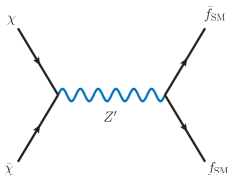
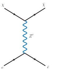
Fig. 1 (a) represents all the possible -channel diagrams contributing to the annihilation cross section of . being a leptophilic neutral gauge boson, can be as long as . For , can’t be accessed. Fig. 1 (b) depicts the DM-electron scattering process mediated by . being charged under with GeV, this particular scattering process is extremely significant to constraint the parameter space through the direct search experiments and DM annihilation at the white dwarfs.
III.1 Relic Density
The vector-like fermion , being a weakly interacting particle [since, ], maintained a thermal equilibrium in the early universe with the SM particles. However, as the universe evolved further, at a certain point in time, the interaction rate of with the SM particles fell short compared to the expansion rate of the universe, and decoupled from the thermal bath. Moreover, being protected against any decay to the SM fields, its abundance was frozen forever to the decoupling value, resulting in its current relic density, . The value can be obtained by solving the Boltzmann equation:
| (9) |
where stands for the number density of with the superscript ‘eq’ representing its equilibrium value. defines the Hubble parameter, and is the thermal averaged annihilation cross section times the relative velocity () of . Note that, since lies in the sub-GeV mass regime, to satisfy the observed relic density near the resonance funnel, one should assume . To be precise, MeV will be considered for all the subsequent discussions. Eq. (9) has been solved numerically using Belanger:2010pz with the model files generated through Semenov:2008jy .
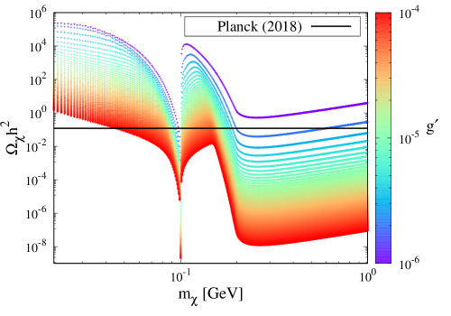
Fig. 2 shows the variation of as a function of with varying continuously between to in steps of . The black solid line marks the observed DM abundance, Planck:2018vyg . Therefore, only those parameter space points in the plane can represent a viable DM candidate for which .
III.2 Direct Detection through DM-Electron Scattering
Direct detection experiments searching for DM-electron scattering are crucial to test the proposed model for two reasons — being non-trivially charged under , can have tree-level interaction only with the first two lepton generations. In the proposed framework, DM-quark scattering will be naturally loop-suppressed, leading to a negligibly small nuclear scattering cross section. The assumption that exists in the sub-GeV mass regime results in a maximal response when scatters on electrons. For a sub-GeV DM, the typical order of energy deposition to the target material varies from eV, which is well below the current sensitivity of the nuclear recoil experiments. However, it is large enough to trigger various atomic processes, e.g., electron ionization, electron excitation, and molecular dissociation. Currently, we have only feasible experimental facilities to probe the electron excitation signals that may arise from a DM scattering event on the regular matter. On an arbitrary target material, the DM scattering rate per unit detector mass can be formulated from the Fermi’s Golden rule as Trickle:2019nya ; Kahn:2021ttr ,
| (10) |
where and are the volume and density of the detector, respectively. defines the DM velocity distribution in the earth frame of reference with GeV/cm3 being the local DM density Catena:2009mf ; Salucci:2010qr . and define the 4-momenta of the incoming and outgoing DM particle , whereas () and () denote the initial and final states (energies) of the target, respectively. Note that, in general, the detector is assumed to be initially in the ground state at zero temperature. Thus, Eq. (10) doesn’t contain a sum over the ensemble of initial states. The interaction between and the target material is described by the non-relativistic (NR) Hamiltonian which can be treated as a perturbation term on the free DM Hamiltonian. The assumption ensures that the unperturbed eigenstates are described by plane wave solutions, and also forbids any entanglement between and the detector states, i.e., and .
In the present framework, DM-target interaction follows from a single effective operator. Therefore, the matrix elements in Eq. (10) can be decomposed as,
| (11) |
where and signify the operators acting only on the target system and DM states, respectively. represents the momentum transfer due to scattering. Using plane wave approximation for the DM states, Eq. (11) results in Kahn:2021ttr ,
| (12) |
Here, and defines the reduced mass of the DM-target 2-body system, with being the mass of the target particle. For DM-electron scattering, . The interaction strength, specific to a DM model, is encapsulated in the effective cross section . However, following the usual convention can be formulated as,
| (13) |
where defines the effective DM-electron elastic scattering cross section. From Fig. 1 (b), it can be calculated as Essig:2011nj ,
| (14) |
with denoting the fine structure constant. Note that, can be interpreted as the cross section for scattering off a free electron with reference momentum keV, after absorbing the momentum dependence of into the DM form factor . At this point, the DM-specific part of the interaction Hamiltonian can be completely described through . However, it’s useful to further factorize Eq. (10) to separate out the target system part. Combining with Eq. (12) and introducing an auxiliary integration variable , Eq. (10) can be recast as,
| (15) |
The entire response of a particular target system towards the DM interaction is now contained within the dynamic structure factor , where the normalization term indicates that is an intrinsic quantity. Since in the present work, interacts only with the electrons in an atomic or solid state detector system, the target-specific effective operator can be defined as, Kaxiras_Joannopoulos_2019 ; Kahn:2021ttr . Here, denotes the position vector of the electron. Thus, the dynamic structure factor reduces to
| (16) |
The detector states , correspond to a generic many-body system and, in general, can’t be momentum eigenstates. Since the analysis majorly focuses on spin-independent NR scattering events, the response of the detector material to the DM can be redefined in terms of the dielectric function , which encodes the response of the material to the EM interactions. Therefore, following Ref. PhysRev.113.1254 , one can obtain,
| (17) |
Note that, if the initial detector state corresponds to a finite temperature , Eq. (17) would have an additional multiplicative factor Girvin_Yang_2019 ; Knapen:2021run ; Hochberg:2021pkt , with representing the Boltzmann constant. However, for , the factor tends to 1, resulting in Eq. (17). The factor is commonly known as the energy loss function (ELF) because it parametrizes the rate of losing energy () and momentum () by a charged particle traversing through the material medium. ELF is an experimentally measured quantity and can be used to compute the DM scattering rate without using any explicit expression for the electron wavefunction within a particular target system. There are two significant advantages of this approach: The non-negligible impact of in-medium screening on the DM scattering rate is automatically included Knapen:2021run ; In the material science literature, ELF is an extremely well-explored parameter. Thus, standard and tested tools exist to extract it for any considered many-body environment.
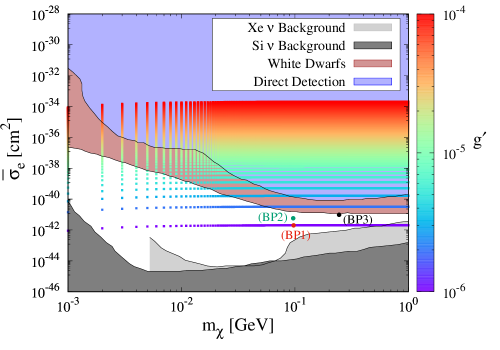
Fig. 3 displays the variation of [i.e., Eq. (14)] as a function of the DM mass with being fixed at 200 MeV. The continuous variation of from to has been depicted as before using the color palette. The light and dark grey shades in Fig. 3 represent the neutrino floor corresponding to Xe and Si targets, respectively Carew:2023qrj . The blue shaded region is a compilation of the direct detection bounds from XENON1T XENON:2019gfn ; XENON:2019zpr , DarkSide-50 DarkSide-50:2022qzh ; DarkSide:2022knj , PandaX-II PandaX-II:2021nsg , and SENSEI SENSEI:2020dpa ; SENSEI:2023zdf . However, for sub-GeV DM, the most stringent bound on can be obtained from DM capture in the white dwarfs. The brown-shaded region defines the parameter space excluded through the observations of white dwarfs in the globular cluster M4 Dasgupta:2019juq ; Bell:2021fye .
Table 2 enlists three benchmark points (BP), which satisfy both relic density and direct detection constraints.
| Parameters | BP1 | BP2 | BP3 |
|---|---|---|---|
| [MeV] | |||
| [MeV] | |||
| [] |
In Fig. 3, these three benchmark points have been labeled with different colors: BP1 (red), BP2 (green), and BP3 (black); the same color code will be followed throughout the paper for representing them graphically. Fig. 4 depicts the variation of differential DM scattering rate for the benchmark points as a function of the deposited energy . The analysis has been executed with a publicly available python-based numerical package, Knapen:2021bwg , which uses the energy loss function to determine DM-electron scattering rate on various possible target materials.
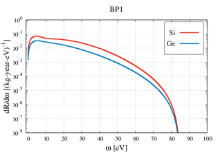
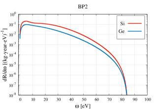
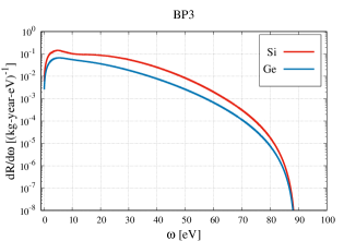
However, for the present purpose, only Si and Ge have been considered. Semiconductor targets are particularly useful for direct detection of sub-GeV DM due to their low bandgap energies. The Mermin oscillator method has been used to generate the variations in Fig. 4. It models the ELF as a weighted linear combination of the ELFs obtained with the Mermin dielectric function Mermin:1970zz . Moreover, the threshold has been set at as for most of the experiments single electron bin may result in a large background. Approximately, the threshold to detect two ionization electrons corresponds to an energy deposition of 4.7 eV and 3.6 eV for Si and Ge, respectively Knapen:2021run ; Essig:2015cda ; 10.1063/1.1656484 , where the differential event rate peaks. Note that, for a particular , Fig. 4 (b), i.e., BP2 shows the highest scattering rate. For BP1, the suppression is due to a smaller value of , whereas for BP3 it comes from a higher . The event rate being inversely proportional to the DM mass, the enhancement due to a larger is nullified in the case of Fig. 4 (c). Moreover, the difference in densities for Si and Ge crystals is also reflected in the respective differential event rates. For cryogenic Si, , whereas for Ge, it is 5.323 Knapen:2021bwg . However, Ge target experiments can probe a comparatively lower mass range due to their smaller bandgap energy.
IV Muon : Reviving the
The anomalous magnetic moment of muon has been determined with a very high degree of precision, both theoretically and experimentally. Thus, any discrepancy between the predicted and measured values of can be considered as a possible signature of some BSM physics. The current SM prediction for the anomalous magnetic moment of muon is given by Aoyama:2020ynm , whereas the 2023 experimental update from the Muon collaboration results in a world average of Muong-2:2023cdq at confidence level. Therefore, the observed discrepancy can be obtained as,
| (18) |
Note that, a recent lattice calculation of the hadronic vacuum polarization (HVP) term by the BMW collaboration Borsanyi:2020mff and a preliminary experimental update from the CMD-3 detector CMD-3:2023alj indicate a notable tension with the present data which may result in a reduced and less significant discrepancy Colangelo:2022jxc between the predicted and observed values of . However, at present, one can only use Eq. (18) to constrain the model parameters.
IV.1 Minimal
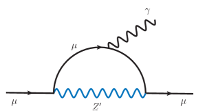
In the minimal model, the only BSM contribution to vertex can be obtained at the one-loop level via , as shown in Fig. 5. In the broken phase of , the corresponding NP correction to can be formulated as Leveille:1977rc ; Baek:2001kca ,
| (19) |
where, .
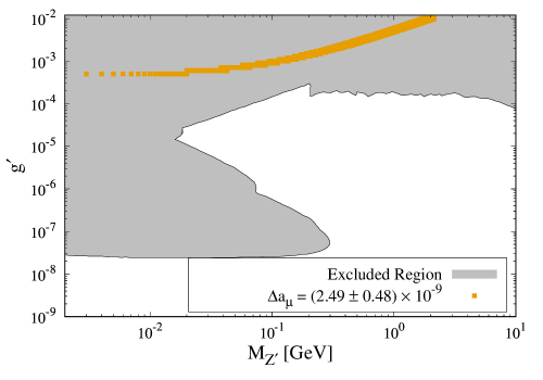
Eq. (19) has been solved numerically with and varying continuously between 1 MeV10 GeV and , respectively. The golden patch in Fig. 6 displays the parameter space where can be explained with Eq. (19), whereas the grey-shaded region shows the parameter space that has already been probed through various experiments, e.g, electron beam dump experiments Riordan:1987aw ; Bjorken:1988as ; Davier:1989wz ; Bross:1989mp ; Bjorken:2009mm ; Andreas:2012mt , electron fixed target experiments APEX:2011dww ; A1:2011yso ; NA64:2016oww , proton beam dump experiments CHARM:1985nku ; LSND:1997vqj ; Blumlein:2011mv ; Blumlein:2013cua , collider searches BaBar:2009lbr ; BaBar:2014zli ; KLOE-2:2011hhj ; KLOE-2:2012lii ; KLOE-2:2016ydq ; Anastasi:2015qla , neutrino experiments Kaneta:2016uyt ; Bilmis:2015lja ; Lindner:2018kjo ; Super-Kamiokande:2011dam ; Ohlsson:2012kf ; Gonzalez-Garcia:2013usa , and white dwarf cooling Dreiner:2013tja . Therefore, in the absence of any positive signal for a hidden gauge sector in the grey region of Fig. 6, the minimal framework has been essentially ruled out as a viable explanation for the observed non-zero .
IV.2 Extended
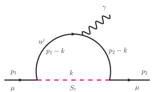
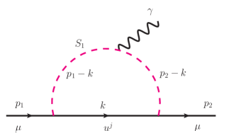
The proposed model extends the minimal particle spectrum with a scalar LQ . Due to the specific charge assignment [see Table 1], couples to muon and the up-type quarks, resulting in the one-loop corrections to the vertex as shown in Fig. 7. Fig. 7 (a) shows the case where the photon couples to the up-type quarks, while Fig. 7 (b) represents the situation when the photon touches the propagator (magenta line). The former will be referred to as Type-1 diagram, while the latter will be called Type-2 for convenience.
Type-1 Diagram
The correction term to vertex due to the Type-1 diagram can be calculated as,
| (20) |
Here, denotes the color multiplicity factor, and represents the EM charge for the up-type quarks in the unit of , i.e., the charge of a proton. stands for the physical mass of the up-type quarks. The numerator of Eq. (20) can be rearranged as,
| (21) |
where,
| (22) |
After Feynman parametrization, the denominator can be recast as,
| (23) |
where and . are the Feynman parameters and . Note that, the calculation assumes an on-shell photon. Moreover, one can easily neglect the muon mass concerning the NP scale involved in the one-loop process. Integrating over the loop momentum , the Type-1 contribution to the muon anomalous magnetic moment can be defined as,
| (24) |
where, the functions and are given by,
| (25) |
Type-2 Diagram
being electromagnetically charged Fig. 7 (b) arises as another contribution to the vertex. The corresponding correction term can be obtained as,
| (26) |
Here is the EM charge of . Recasting the numerator of Eq. (26), one gets,
| (27) |
Using Feynman parametrization, the denominator can be redefined as,
| (28) |
Thus, the Type-2 diagram contributes to the muon anomalous magnetic moment as,
| (29) |
where,
| (30) |
Therefore, in the presence of a scalar LQ , transforming non-trivially under , the leading order NP contribution to can be defined as,
| (31) |
where can be read from Eq. (19). Note that, for any set of parameter points, Fig. 7 (a) and 7 (b) result in oppositely aligned contributions. Therefore, the sum must be so adjusted that one obtains within allowed regions of plane.
Numerical Analysis
In the extended model, the parameter space relevant for describing the , is given by,
with . Thus, there is a 9-dimensional parameter space in total. However, can be fixed at 2 TeV to simplify the numerical analysis without losing any physically significant outcome. The choice is completely in accordance with the collider bounds for generation scalar LQs ParticleDataGroup:2022pth . Moreover, in the absence of CLFV processes, the NP couplings and are unconstrained over the entire parameter space for all the quark generations. Therefore, to reduce the computational rigor, the flavor index can be suppressed, and one can assume , and . Note that, considering the quark-specific generation index will just enhance the degrees of freedom without any notable phenomenological effect.
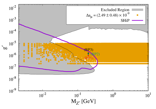
Fig. 8 shows the plane for the extended framework. As before, the grey-shaded portion of the plot denotes the excluded regions of the parameter space. The crucial impact of having a scalar LQ charged under is that the model can explain over the entire plane. In case of a subdominant contribution from Fig. 5, Fig. 7 generates the compensating correction such that can always be explained with Eq. (31). However, for the present purpose, has been varied continuously from to for each value between 1 MeV to 10 GeV. The LQ Yukawa couplings and have been varied randomly between for each of the data point. The results have been shown with the golden dots in Fig. 8. Following the aforementioned color convention, BP1, BP2, and BP3 have been marked with red, green, and black, respectively. Therefore, the three benchmark points can also explain the observed along with the DM phenomenology. Moreover, they are within the reach of the proposed SHiP experiment SHiP:2015vad ; Alekhin:2015byh ; SHiP:2021nfo . The projected bound has been outlined with violet in Fig. 8.
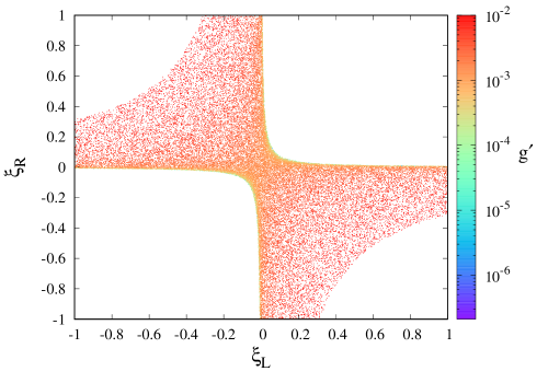
Fig. 9 displays a scatter plot in the plane. Here, has been fixed at 200 MeV and varies continuously from to . Note that, the range of has been chosen for a general purpose, and hence, the experimental bounds [see Fig. 8] have not been considered here. However, one can always extract the allowed parameter space from Fig. 9. It’s interesting to note that for smaller values (approximately, ), , whereas the product turns to be negative in the higher range of . For with MeV, Eq. (19) results in . Therefore, a major compensation must come from to explain the observed discrepancy. However, not all the terms of and contribute equally. It can be easily checked that for , the functions follow the hierarchy: . Moreover, the first terms of Eqs. (24) and (29) are suppressed by a factor of . Thus, the leading order contribution from effectively depends on the second term of Eq. (24), i.e., . It clearly implies that for , has to be positive, while for , . In practice, for the latter case, corresponds to only. In case of , can only be set within the observed range if . Note that, with , it is impossible to create a negative contribution from due to the order of dominance between and . However, only the first case, i.e., is phenomenologically relevant; and correspond to the experimentally excluded regions of the parameter space.
V Conclusions
The paper primarily addresses one of the major issues with all the extensions of the SM. Though these well-motivated BSM theories provide a quite natural explanation for the observed discrepancies in lepton , the associated parameter spaces have either been excluded or are on the verge of being probed through various experiments. The situation is particularly severe for . Thus, the proposed model extends the minimal particle spectrum of theory with a scalar LQ , transforming as under the considered gauge group. The NP interaction between quarks and leptons is assumed to arise at the TeV scale. Such a theory has strong GUT motivation and is within the reach of the future high-energy colliders. Note that, the charge assignment of is specifically chosen to explain within the experimentally allowed parameter space. can also be explained using the same framework if one assigns a -charge of to the LQ. However, for a simultaneous explanation of and , the assumed particle spectrum has to be extended further as a single LQ charged under can’t couple to both electron and muon at the same time. The possibility is beyond the scope of the present work and can be explored in the future. In the considered model, can couple only the muon to the up-type quarks, leading to additional BSM contributions to . These NP corrections compensate for the minimal model as it produces a much-suppressed contribution to in the allowed parameter space. Thus, in the presence of a TeV-scale scalar LQ , gauge formulation can effectively be revived over the entire allowed region of plane as a natural theory for . Note that, though has been considered here for analysis, the conclusions are generic and applicable for any of the theory with a proper charge assignment of .
In addition to , the model can also explain the observed DM abundance and the direct detection results. A vector-like SM-singlet fermion with a non-zero charge has been introduced as a viable DM candidate. Further, the model being naturally favorable for DM-electron scattering, has been restricted to the sub-GeV mass regime so that the DM-specific parameter space can be efficiently constrained through the direct detection and white dwarf bounds on . Following the numerical results, three benchmark points have been chosen that satisfy both the relic density and direct detection constraints and thus represent testable parameter space points for the DM phenomenology. The actual detection prospects of have been predicted for Si and Ge-based detectors as they are more suitable for sub-GeV DM compared to the noble gas detectors. Due to band formation, semiconductors feature a better detection probability for light DM candidates. Out of the three benchmark points, BP2 is found to have a higher differential scattering rate. However, all three benchmark points satisfy and correspond to a parameter space that can be probed with the future SHiP facility. Therefore, the direct detection experiments and searches for a hidden gauge sector can be used in complementarity of each other to test/falsify the model.
References
- (1) ATLAS collaboration, G. Aad et al., Observation of a new particle in the search for the Standard Model Higgs boson with the ATLAS detector at the LHC, Phys. Lett. B 716 (2012) 1–29, [1207.7214].
- (2) CMS collaboration, S. Chatrchyan et al., Observation of a New Boson at a Mass of 125 GeV with the CMS Experiment at the LHC, Phys. Lett. B 716 (2012) 30–61, [1207.7235].
- (3) ATLAS collaboration, G. Aad et al., Measurement of the W-boson mass and width with the ATLAS detector using proton-proton collisions at = 7 TeV, 2403.15085.
- (4) CMS collaboration, Measurement of the W boson mass in proton-proton collisions at TeV, tech. rep., CERN, Geneva, 2024.
- (5) J. H. Oort, The force exerted by the stellar system in the direction perpendicular to the galactic plane and some related problems, Bulletin of the Astronomical Institutes of the Netherlands 6 (Aug., 1932) 249.
- (6) F. Zwicky, Die Rotverschiebung von extragalaktischen Nebeln, Helv. Phys. Acta 6 (1933) 110–127.
- (7) F. Zwicky, On the Masses of Nebulae and of Clusters of Nebulae, Astrophys. J. 86 (1937) 217–246.
- (8) R. B. Metcalf, L. A. Moustakas, A. J. Bunker and I. R. Parry, Spectroscopic gravitational lensing and limits on the dark matter substructure in Q2237+0305, Astrophys. J. 607 (2004) 43–59, [astro-ph/0309738].
- (9) Planck collaboration, N. Aghanim et al., Planck 2018 results. VI. Cosmological parameters, Astron. Astrophys. 641 (2020) A6, [1807.06209]. [Erratum: Astron.Astrophys. 652, C4 (2021)].
- (10) Muon g-2 collaboration, D. P. Aguillard et al., Measurement of the Positive Muon Anomalous Magnetic Moment to 0.20 ppm, Phys. Rev. Lett. 131 (2023) 161802, [2308.06230].
- (11) R. H. Parker, C. Yu, W. Zhong, B. Estey and H. Müller, Measurement of the fine-structure constant as a test of the Standard Model, Science 360 (2018) 191, [1812.04130].
- (12) L. Morel, Z. Yao, P. Cladé and S. Guellati-Khélifa, Determination of the fine-structure constant with an accuracy of 81 parts per trillion, Nature 588 (2020) 61–65.
- (13) B. Pontecorvo, Neutrino Experiments and the Problem of Conservation of Leptonic Charge, Zh. Eksp. Teor. Fiz. 53 (1967) 1717–1725.
- (14) T. Aoyama et al., The anomalous magnetic moment of the muon in the Standard Model, Phys. Rept. 887 (2020) 1–166, [2006.04822].
- (15) P. Langacker, The Physics of Heavy Gauge Bosons, Rev. Mod. Phys. 81 (2009) 1199–1228, [0801.1345].
- (16) R. W. Robinett and J. L. Rosner, Mass Scales in Grand Unified Theories, Phys. Rev. D 26 (1982) 2396.
- (17) P. Langacker, R. W. Robinett and J. L. Rosner, New Heavy Gauge Bosons in p p and p anti-p Collisions, Phys. Rev. D 30 (1984) 1470.
- (18) I. Antoniadis, A Possible new dimension at a few TeV, Phys. Lett. B 246 (1990) 377–384.
- (19) T. Appelquist, H.-C. Cheng and B. A. Dobrescu, Bounds on universal extra dimensions, Phys. Rev. D 64 (2001) 035002, [hep-ph/0012100].
- (20) M. Goodsell and A. Ringwald, Light Hidden-Sector U(1)s in String Compactifications, Fortsch. Phys. 58 (2010) 716–720, [1002.1840].
- (21) R. Foot, New Physics From Electric Charge Quantization?, Mod. Phys. Lett. A 6 (1991) 527–530.
- (22) X.-G. He, G. C. Joshi, H. Lew and R. R. Volkas, Simplest Z-prime model, Phys. Rev. D 44 (1991) 2118–2132.
- (23) R. Foot, X. G. He, H. Lew and R. R. Volkas, Model for a light Z-prime boson, Phys. Rev. D 50 (1994) 4571–4580, [hep-ph/9401250].
- (24) E. M. Riordan et al., A Search for Short Lived Axions in an Electron Beam Dump Experiment, Phys. Rev. Lett. 59 (1987) 755.
- (25) J. D. Bjorken, S. Ecklund, W. R. Nelson, A. Abashian, C. Church, B. Lu et al., Search for Neutral Metastable Penetrating Particles Produced in the SLAC Beam Dump, Phys. Rev. D 38 (1988) 3375.
- (26) M. Davier and H. Nguyen Ngoc, An Unambiguous Search for a Light Higgs Boson, Phys. Lett. B 229 (1989) 150–155.
- (27) A. Bross, M. Crisler, S. H. Pordes, J. Volk, S. Errede and J. Wrbanek, A Search for Shortlived Particles Produced in an Electron Beam Dump, Phys. Rev. Lett. 67 (1991) 2942–2945.
- (28) J. D. Bjorken, R. Essig, P. Schuster and N. Toro, New Fixed-Target Experiments to Search for Dark Gauge Forces, Phys. Rev. D 80 (2009) 075018, [0906.0580].
- (29) S. Andreas, C. Niebuhr and A. Ringwald, New Limits on Hidden Photons from Past Electron Beam Dumps, Phys. Rev. D 86 (2012) 095019, [1209.6083].
- (30) APEX collaboration, S. Abrahamyan et al., Search for a New Gauge Boson in Electron-Nucleus Fixed-Target Scattering by the APEX Experiment, Phys. Rev. Lett. 107 (2011) 191804, [1108.2750].
- (31) A1 collaboration, H. Merkel et al., Search for Light Gauge Bosons of the Dark Sector at the Mainz Microtron, Phys. Rev. Lett. 106 (2011) 251802, [1101.4091].
- (32) NA64 collaboration, D. Banerjee et al., Search for invisible decays of sub-GeV dark photons in missing-energy events at the CERN SPS, Phys. Rev. Lett. 118 (2017) 011802, [1610.02988].
- (33) CHARM collaboration, F. Bergsma et al., A Search for Decays of Heavy Neutrinos in the Mass Range 0.5-GeV to 2.8-GeV, Phys. Lett. B 166 (1986) 473–478.
- (34) LSND collaboration, C. Athanassopoulos et al., Evidence for muon-neutrino — electron-neutrino oscillations from pion decay in flight neutrinos, Phys. Rev. C 58 (1998) 2489–2511, [nucl-ex/9706006].
- (35) J. Blumlein and J. Brunner, New Exclusion Limits for Dark Gauge Forces from Beam-Dump Data, Phys. Lett. B 701 (2011) 155–159, [1104.2747].
- (36) J. Blümlein and J. Brunner, New Exclusion Limits on Dark Gauge Forces from Proton Bremsstrahlung in Beam-Dump Data, Phys. Lett. B 731 (2014) 320–326, [1311.3870].
- (37) BaBar collaboration, B. Aubert et al., Search for Dimuon Decays of a Light Scalar Boson in Radiative Transitions Upsilon — gamma A0, Phys. Rev. Lett. 103 (2009) 081803, [0905.4539].
- (38) BaBar collaboration, J. P. Lees et al., Search for a Dark Photon in Collisions at BaBar, Phys. Rev. Lett. 113 (2014) 201801, [1406.2980].
- (39) KLOE-2 collaboration, F. Archilli et al., Search for a vector gauge boson in meson decays with the KLOE detector, Phys. Lett. B 706 (2012) 251–255, [1110.0411].
- (40) KLOE-2 collaboration, D. Babusci et al., Limit on the production of a light vector gauge boson in phi meson decays with the KLOE detector, Phys. Lett. B 720 (2013) 111–115, [1210.3927].
- (41) KLOE-2 collaboration, A. Anastasi et al., Limit on the production of a new vector boson in , U with the KLOE experiment, Phys. Lett. B 757 (2016) 356–361, [1603.06086].
- (42) A. Anastasi et al., Limit on the production of a low-mass vector boson in , with the KLOE experiment, Phys. Lett. B 750 (2015) 633–637, [1509.00740].
- (43) Y. Kaneta and T. Shimomura, On the possibility of a search for the gauge boson at Belle-II and neutrino beam experiments, PTEP 2017 (2017) 053B04, [1701.00156].
- (44) S. Bilmis, I. Turan, T. M. Aliev, M. Deniz, L. Singh and H. T. Wong, Constraints on Dark Photon from Neutrino-Electron Scattering Experiments, Phys. Rev. D 92 (2015) 033009, [1502.07763].
- (45) M. Lindner, F. S. Queiroz, W. Rodejohann and X.-J. Xu, Neutrino-electron scattering: general constraints on Z′ and dark photon models, JHEP 05 (2018) 098, [1803.00060].
- (46) Super-Kamiokande collaboration, G. Mitsuka et al., Study of Non-Standard Neutrino Interactions with Atmospheric Neutrino Data in Super-Kamiokande I and II, Phys. Rev. D 84 (2011) 113008, [1109.1889].
- (47) T. Ohlsson, Status of non-standard neutrino interactions, Rept. Prog. Phys. 76 (2013) 044201, [1209.2710].
- (48) M. C. Gonzalez-Garcia and M. Maltoni, Determination of matter potential from global analysis of neutrino oscillation data, JHEP 09 (2013) 152, [1307.3092].
- (49) H. K. Dreiner, J.-F. Fortin, J. Isern and L. Ubaldi, White Dwarfs constrain Dark Forces, Phys. Rev. D 88 (2013) 043517, [1303.7232].
- (50) M. Bauer, P. Foldenauer and J. Jaeckel, Hunting All the Hidden Photons, JHEP 07 (2018) 094, [1803.05466].
- (51) A. Greljo, P. Stangl, A. E. Thomsen and J. Zupan, On (g 2)μ from gauged U(1)X, JHEP 07 (2022) 098, [2203.13731].
- (52) I. Dors̆ner, S. Fajfer, A. Greljo, J. F. Kamenik and N. Kos̆nik, Physics of leptoquarks in precision experiments and at particle colliders, Phys. Rept. 641 (2016) 1–68, [1603.04993].
- (53) J. C. Pati and A. Salam, Lepton Number as the Fourth Color, Phys. Rev. D 10 (1974) 275–289. [Erratum: Phys.Rev.D 11, 703–703 (1975)].
- (54) H. Georgi and S. L. Glashow, Unity of All Elementary Particle Forces, Phys. Rev. Lett. 32 (1974) 438–441.
- (55) H. Georgi, The State of the Art—Gauge Theories, AIP Conf. Proc. 23 (1975) 575–582.
- (56) I. Dors̆ner, S. Fajfer, N. Kos̆nik and I. Nis̆andz̆ić, Minimally flavored colored scalar in and the mass matrices constraints, JHEP 11 (2013) 084, [1306.6493].
- (57) B. Gripaios, M. Nardecchia and S. A. Renner, Composite leptoquarks and anomalies in -meson decays, JHEP 05 (2015) 006, [1412.1791].
- (58) D. Bečirević, S. Fajfer and N. Kos̆nik, Lepton flavor nonuniversality in processes, Phys. Rev. D92 (2015) 014016, [1503.09024].
- (59) D. Bečirević, S. Fajfer, N. Kos̆nik and O. Sumensari, Leptoquark model to explain the -physics anomalies, and , Phys. Rev. D94 (2016) 115021, [1608.08501].
- (60) A. Crivellin, D. Müller and T. Ota, Simultaneous explanation of and : the last scalar leptoquarks standing, JHEP 09 (2017) 040, [1703.09226].
- (61) J. M. Cline, decay anomalies and dark matter from vectorlike confinement, Phys. Rev. D97 (2018) 015013, [1710.02140].
- (62) L. Di Luzio and M. Nardecchia, What is the scale of new physics behind the -flavour anomalies?, Eur. Phys. J. C77 (2017) 536, [1706.01868].
- (63) T. Mandal, S. Mitra and S. Raz, motivated leptoquark scenarios: Impact of interference on the exclusion limits from LHC data, Phys. Rev. D99 (2019) 055028, [1811.03561].
- (64) U. Aydemir, T. Mandal and S. Mitra, Addressing the anomalies with an leptoquark from grand unification, Phys. Rev. D101 (2020) 015011, [1902.08108].
- (65) A. Crivellin, D. Müller and F. Saturnino, Flavor Phenomenology of the Leptoquark Singlet-Triplet Model, 1912.04224.
- (66) P. Asadi, A. Bhattacharya, K. Fraser, S. Homiller and A. Parikh, Wrinkles in the Froggatt-Nielsen Mechanism and Flavorful New Physics, 2308.01340.
- (67) K. Cheung, W. Y. Keung and P. Y. Tseng, Leptoquark induced rare decay amplitudes and , Phys. Rev. D 93 (2016) 015010, [1508.01897].
- (68) R. Mandal and A. Pich, Constraints on scalar leptoquarks from lepton and kaon physics, JHEP 12 (2019) 089, [1908.11155].
- (69) B. De, Leptoquark-induced CLFV decays with a light SM-singlet scalar, Phys. Lett. B 855 (2024) 138784, [2405.06970].
- (70) R. Mandal, Fermionic dark matter in leptoquark portal, Eur. Phys. J. C78 (2018) 726, [1808.07844].
- (71) S.-M. Choi, Y.-J. Kang, H. M. Lee and T.-G. Ro, Lepto-Quark Portal Dark Matter, JHEP 10 (2018) 104, [1807.06547].
- (72) A. Mohamadnejad, Accidental scale-invariant Majorana dark matter in leptoquark-Higgs portals, Nucl. Phys. B 949 (2019) 114793, [1904.03857].
- (73) A. Bhaskar, D. Das, B. De and S. Mitra, Enhancing scalar productions with leptoquarks at the LHC, Phys. Rev. D 102 (2020) 035002, [2002.12571].
- (74) A. Bhaskar, D. Das, B. De, S. Mitra, A. K. Nayak and C. Neeraj, Leptoquark-assisted singlet-mediated di-Higgs production at the LHC, Phys. Lett. B 833 (2022) 137341, [2205.12210].
- (75) L. Da Rold, M. Epele, A. Medina, N. I. Mileo and A. Szynkman, Enhancement of the double Higgs production via leptoquarks at the LHC, JHEP 08 (2021) 100, [2105.06309].
- (76) P. Agrawal and U. Mahanta, Leptoquark contribution to the Higgs boson production at the CERN LHC collider, Phys. Rev. D 61 (2000) 077701, [hep-ph/9911497].
- (77) T. Enkhbat, Scalar leptoquarks and Higgs pair production at the LHC, JHEP 01 (2014) 158, [1311.4445].
- (78) B. De, Direct production of SM-singlet scalars at the muon collider, Phys. Lett. B 852 (2024) 138634, [2401.08101].
- (79) A. Djouadi, T. Köhler, M. Spira and J. Tutas, (eb), (et) type leptoquarks atep colliders, Zeitschrift für Physik C Particles and Fields 46 (Dec, 1990) 679–685.
- (80) K.-m. Cheung, Muon anomalous magnetic moment and leptoquark solutions, Phys. Rev. D64 (2001) 033001, [hep-ph/0102238].
- (81) I. Doršner, S. Fajfer and O. Sumensari, Muon and scalar leptoquark mixing, 1910.03877.
- (82) B. De, Revisiting the scalar leptoquark model with the updated leptonic constraints, Eur. Phys. J. C 83 (2023) 1084, [2310.01778].
- (83) W. Buchmuller and D. Wyler, Constraints on su(5)-type leptoquarks, Physics Letters B 177 (1986) 377 – 382.
- (84) H. Murayama and T. Yanagida, A viable SU(5) GUT with light leptoquark bosons, Mod. Phys. Lett. A 7 (1992) 147–152.
- (85) I. Dorsner and P. Fileviez Perez, Unification without supersymmetry: Neutrino mass, proton decay and light leptoquarks, Nucl. Phys. B 723 (2005) 53–76, [hep-ph/0504276].
- (86) H. Georgi and C. Jarlskog, A new lepton-quark mass relation in a unified theory, Physics Letters B 86 (1979) 297–300.
- (87) P. Fileviez Perez, Renormalizable adjoint SU(5), Phys. Lett. B 654 (2007) 189–193, [hep-ph/0702287].
- (88) G. Senjanovic and A. Sokorac, Light Leptoquarks in SO(10), Z. Phys. C 20 (1983) 255.
- (89) I. Dorsner and P. Fileviez Perez, Could we rotate proton decay away?, Phys. Lett. B 606 (2005) 367–370, [hep-ph/0409190].
- (90) I. Doršner and S. Saad, Is Doublet-Triplet Splitting Necessary?, 2404.09021.
- (91) G. Bertone, D. Hooper and J. Silk, Particle dark matter: Evidence, candidates and constraints, Phys. Rept. 405 (2005) 279–390, [hep-ph/0404175].
- (92) G. Jungman, M. Kamionkowski and K. Griest, Supersymmetric dark matter, Phys. Rept. 267 (1996) 195–373, [hep-ph/9506380].
- (93) P. Gondolo and G. Gelmini, Cosmic abundances of stable particles: Improved analysis, Nuclear Physics B 360 (1991) 145–179.
- (94) M. Cirelli, A. Strumia and J. Zupan, Dark Matter, 2406.01705.
- (95) J. L. Hewett and T. G. Rizzo, Low-Energy Phenomenology of Superstring Inspired E(6) Models, Phys. Rept. 183 (1989) 193.
- (96) P. Langacker, Grand Unified Theories and Proton Decay, Phys. Rept. 72 (1981) 185.
- (97) P. Minkowski, at a Rate of One Out of Muon Decays?, Phys. Lett. B 67 (1977) 421–428.
- (98) R. Foot, H. Lew, X. G. He and G. C. Joshi, Seesaw Neutrino Masses Induced by a Triplet of Leptons, Z. Phys. C 44 (1989) 441.
- (99) R. Essig, J. Mardon and T. Volansky, Direct Detection of Sub-GeV Dark Matter, Phys. Rev. D 85 (2012) 076007, [1108.5383].
- (100) P. W. Graham, D. E. Kaplan, S. Rajendran and M. T. Walters, Semiconductor Probes of Light Dark Matter, Phys. Dark Univ. 1 (2012) 32–49, [1203.2531].
- (101) R. Essig, M. Fernandez-Serra, J. Mardon, A. Soto, T. Volansky and T.-T. Yu, Direct Detection of sub-GeV Dark Matter with Semiconductor Targets, JHEP 05 (2016) 046, [1509.01598].
- (102) P. Foldenauer, Light dark matter in a gauged model, Phys. Rev. D 99 (2019) 035007, [1808.03647].
- (103) B. Dutta, S. Ghosh and J. Kumar, A sub-GeV dark matter model, Phys. Rev. D 100 (2019) 075028, [1905.02692].
- (104) S. Knapen, J. Kozaczuk and T. Lin, Dark matter-electron scattering in dielectrics, Phys. Rev. D 104 (2021) 015031, [2101.08275].
- (105) Y. Hochberg, Y. Kahn, N. Kurinsky, B. V. Lehmann, T. C. Yu and K. K. Berggren, Determining Dark-Matter–Electron Scattering Rates from the Dielectric Function, Phys. Rev. Lett. 127 (2021) 151802, [2101.08263].
- (106) Y. Kahn and T. Lin, Searches for light dark matter using condensed matter systems, Rept. Prog. Phys. 85 (2022) 066901, [2108.03239].
- (107) M. Chen, G. B. Gelmini and V. Takhistov, Halo-independent dark matter electron scattering analysis with in-medium effects, Phys. Lett. B 841 (2023) 137922, [2209.10902].
- (108) B. Barman, A. Das and S. Mandal, Dark matter-electron scattering and freeze-in scenarios in the light of Z’ mediation, Phys. Rev. D 110 (2024) 055029, [2407.00969].
- (109) K. Kannike, Vacuum Stability Conditions From Copositivity Criteria, Eur. Phys. J. C 72 (2012) 2093, [1205.3781].
- (110) Particle Data Group collaboration, R. L. Workman et al., Review of Particle Physics, PTEP 2022 (2022) 083C01.
- (111) ATLAS collaboration, G. Aad et al., Search for invisible Higgs-boson decays in events with vector-boson fusion signatures using 139 fb-1 of proton-proton data recorded by the ATLAS experiment, JHEP 08 (2022) 104, [2202.07953].
- (112) P. Ballett, M. Hostert, S. Pascoli, Y. F. Perez-Gonzalez, Z. Tabrizi and R. Zukanovich Funchal, s in neutrino scattering at DUNE, Phys. Rev. D 100 (2019) 055012, [1902.08579].
- (113) M. Ardu and F. Kirk, A viable model with violation, Eur. Phys. J. C 83 (2023) 394, [2205.02254].
- (114) A. Dasgupta, P. S. B. Dev, T. Han, R. Padhan, S. Wang and K. Xie, Searching for heavy leptophilic Z’: from lepton colliders to gravitational waves, JHEP 12 (2023) 011, [2308.12804].
- (115) G. Belanger, F. Boudjema, A. Pukhov and A. Semenov, micrOMEGAs: A Tool for dark matter studies, Nuovo Cim. C 033N2 (2010) 111–116, [1005.4133].
- (116) A. Semenov, LanHEP: A Package for the automatic generation of Feynman rules in field theory. Version 3.0, Comput. Phys. Commun. 180 (2009) 431–454, [0805.0555].
- (117) T. Trickle, Z. Zhang, K. M. Zurek, K. Inzani and S. M. Griffin, Multi-Channel Direct Detection of Light Dark Matter: Theoretical Framework, JHEP 03 (2020) 036, [1910.08092].
- (118) R. Catena and P. Ullio, A novel determination of the local dark matter density, JCAP 08 (2010) 004, [0907.0018].
- (119) P. Salucci, F. Nesti, G. Gentile and C. F. Martins, The dark matter density at the Sun’s location, Astron. Astrophys. 523 (2010) A83, [1003.3101].
- (120) E. Kaxiras and J. D. Joannopoulos, Quantum Theory of Materials. Cambridge University Press, 2019.
- (121) P. Nozières and D. Pines, Electron interaction in solids. characteristic energy loss spectrum, Phys. Rev. 113 (Mar, 1959) 1254–1267.
- (122) S. M. Girvin and K. Yang, Modern Condensed Matter Physics. Cambridge University Press, 2019.
- (123) B. Carew, A. R. Caddell, T. N. Maity and C. A. J. O’Hare, Neutrino fog for dark matter-electron scattering experiments, Phys. Rev. D 109 (2024) 083016, [2312.04303].
- (124) XENON collaboration, E. Aprile et al., Light Dark Matter Search with Ionization Signals in XENON1T, Phys. Rev. Lett. 123 (2019) 251801, [1907.11485].
- (125) XENON collaboration, E. Aprile et al., Search for Light Dark Matter Interactions Enhanced by the Migdal Effect or Bremsstrahlung in XENON1T, Phys. Rev. Lett. 123 (2019) 241803, [1907.12771].
- (126) DarkSide-50 collaboration, P. Agnes et al., Search for low-mass dark matter WIMPs with 12 ton-day exposure of DarkSide-50, Phys. Rev. D 107 (2023) 063001, [2207.11966].
- (127) DarkSide collaboration, P. Agnes et al., Search for Dark Matter Particle Interactions with Electron Final States with DarkSide-50, Phys. Rev. Lett. 130 (2023) 101002, [2207.11968].
- (128) PandaX-II collaboration, C. Cheng et al., Search for Light Dark Matter-Electron Scatterings in the PandaX-II Experiment, Phys. Rev. Lett. 126 (2021) 211803, [2101.07479].
- (129) SENSEI collaboration, L. Barak et al., SENSEI: Direct-Detection Results on sub-GeV Dark Matter from a New Skipper-CCD, Phys. Rev. Lett. 125 (2020) 171802, [2004.11378].
- (130) SENSEI collaboration, P. Adari et al., SENSEI: First Direct-Detection Results on sub-GeV Dark Matter from SENSEI at SNOLAB, 2312.13342.
- (131) B. Dasgupta, A. Gupta and A. Ray, Dark matter capture in celestial objects: Improved treatment of multiple scattering and updated constraints from white dwarfs, JCAP 08 (2019) 018, [1906.04204].
- (132) N. F. Bell, G. Busoni, M. E. Ramirez-Quezada, S. Robles and M. Virgato, Improved treatment of dark matter capture in white dwarfs, JCAP 10 (2021) 083, [2104.14367].
- (133) S. Knapen, J. Kozaczuk and T. Lin, python package for dark matter scattering in dielectric targets, Phys. Rev. D 105 (2022) 015014, [2104.12786].
- (134) N. D. Mermin, Lindhard Dielectric Function in the Relaxation-Time Approximation, Phys. Rev. B 1 (1970) 2362–2363.
- (135) C. A. Klein, Bandgap Dependence and Related Features of Radiation Ionization Energies in Semiconductors, Journal of Applied Physics 39 (03, 1968) 2029–2038, [https://pubs.aip.org/aip/jap/article-pdf/39/4/2029/18345797/2029_1_online.pdf].
- (136) S. Borsanyi et al., Leading hadronic contribution to the muon magnetic moment from lattice QCD, Nature 593 (2021) 51–55, [2002.12347].
- (137) CMD-3 collaboration, F. V. Ignatov et al., Measurement of the cross section from threshold to 1.2 GeV with the CMD-3 detector, 2302.08834.
- (138) G. Colangelo et al., Prospects for precise predictions of in the Standard Model, 2203.15810.
- (139) J. P. Leveille, The Second Order Weak Correction to (G-2) of the Muon in Arbitrary Gauge Models, Nucl. Phys. B 137 (1978) 63–76.
- (140) S. Baek, N. G. Deshpande, X. G. He and P. Ko, Muon anomalous g-2 and gauged L(muon) - L(tau) models, Phys. Rev. D 64 (2001) 055006, [hep-ph/0104141].
- (141) SHiP collaboration, M. Anelli et al., A facility to Search for Hidden Particles (SHiP) at the CERN SPS, 1504.04956.
- (142) S. Alekhin et al., A facility to Search for Hidden Particles at the CERN SPS: the SHiP physics case, Rept. Prog. Phys. 79 (2016) 124201, [1504.04855].
- (143) SHiP collaboration, C. Ahdida et al., The SHiP experiment at the proposed CERN SPS Beam Dump Facility, Eur. Phys. J. C 82 (2022) 486, [2112.01487].