Efficient, Cross-Fitting Estimation of Semiparametric Spatial Point Processes

Abstract

We study a broad class of models called semiparametric spatial point processes where the first-order intensity function contains both a parametric component and a nonparametric component. We propose a novel, spatial cross-fitting estimator of the parametric component based on random thinning, a common simulation technique in point processes. The proposed estimator is shown to be consistent and in many settings, asymptotically Normal. Also, we generalize the notion of semiparametric efficiency lower bound in i.i.d. settings to spatial point processes and show that the proposed estimator achieves the efficiency lower bound if the process is Poisson. Next, we present a new spatial kernel regression estimator that can estimate the nonparametric component of the intensity function at the desired rates for inference. Despite the dependence induced by the point process, we show that our estimator can be computed using existing software for generalized partial linear models in i.i.d. settings. We conclude with a small simulation study and a re-analysis of the spatial distribution of rainforest trees.

Keywords: Inhomogeneous spatial point processes, generalized partial linear models, semiparametric efficiency lower bound, thinning.

1 Introduction

Parametric spatial point processes are widely used to quantify the relationship between the spatial distribution of events, for instance, the location of trees, violent crime, or gene expressions in a cell, and relevant spatial covariates, such as elevation, socioeconomic characteristics of a neighborhood, or cellular environment; see Baddeley et al., (2015) for textbook examples. Specifically, the intensity function $\lambda(\cdot)$, which governs the spatial distribution of events, is a parametric function of the spatial covariates, for example, $\lambda(\mathbf{u};\boldsymbol{\theta})=\exp\left[\boldsymbol{\theta}^{\top}\mathbf{y}(\mathbf{u})\right]$ where $\mathbf{u}$ is the spatial location in $\mathbb{R}^{2}$, $\mathbf{y}(\mathbf{u})$ are the values of the spatial covariates at location $\mathbf{u}$, and $\boldsymbol{\theta}$ quantifies the relationship between the spatial covariates and the spatial distribution of events. Rathbun and Cressie, (1994) showed that the maximum likelihood estimator (MLE) of $\boldsymbol{\theta}$ is consistent, asymptotically Normal, and statistically efficient when the point process is Poisson, i.e., the number of spatial events observed in non-overlapping spatial regions is independent. Later, Schoenberg, (2005), Guan and Loh, (2007), and Waagepetersen and Guan, (2009) showed that the MLE in Rathbun and Cressie, (1994) remained consistent and asymptotically Normal even if the process is not Poisson, but with a loss in statistical efficiency. Also, Berman and Turner, (1992), Baddeley and Turner, (2000), and Baddeley et al., (2014) proposed computationally efficient approaches to compute the MLE. These methods for parametric spatial point processes are widely accessible with the R package spatstat (Baddeley and Turner,, 2005).

The main theme of the paper is to propose a more general class of models that study the same questions as above (i.e., the relationship between spatial events and spatial covariates), but with less restrictive modeling assumptions and without sacrificing the aforementioned statistical and computational properties (i.e., consistency, asymptotic Normality, statistical and computational efficiency). Formally, suppose we partition the set of spatial covariates into two types, $\mathbf{y}_{\mathbf{u}}:=\mathbf{y}(\mathbf{u})$ and $\mathbf{z}_{\mathbf{u}}:=\mathbf{z}(\mathbf{u})$, and the intensity function takes the form

$$\lambda(\mathbf{u};\boldsymbol{\theta},\eta)=\Psi\left[\tau_{\boldsymbol{\theta}}(\mathbf{y}_{\mathbf{u}}),\eta(\mathbf{z}_{\mathbf{u}})\right],\quad{}\boldsymbol{\theta}\in\Theta,\eta\in\mathcal{H}.$$ (1)

The term $\tau_{\boldsymbol{\theta}}(\cdot)$ is an user-specified function of $\mathbf{y}$ and is parameterized by the finite-dimensional parameter $\boldsymbol{\theta}$ in some Euclidean space $\Theta$, for instance $\tau_{\boldsymbol{\theta}}(\mathbf{y}_{\mathbf{u}})=\boldsymbol{\theta}^{\top}\mathbf{y}_{\mathbf{u}}$ and $\boldsymbol{\theta}$ is a vector of real numbers. The term $\eta(\cdot)$ is an unknown, infinite-dimensional function of $\mathbf{z}_{\mathbf{u}}$ in a linear space $\mathcal{H}$, for instance the space of smooth functions in a Hilbert space. The function $\Psi(\cdot)$ is a user-specified link function and a popular choice is the exponential function. The class of spatial point processes with an intensity function in (1), which we refer to as a semiparametric spatial point process, encompasses a variety of existing models, including: (a) the parametric spatial point process mentioned above, (b) spatial point processes of the form $\lambda(\mathbf{u})=\lambda_{0}(\mathbf{u})\exp\left[\boldsymbol{\theta}^{\top}\mathbf{y}(\mathbf{u})\right]$ where $\lambda_{0}(\mathbf{u})$ is a nonparametric, “baseline” rate/intensity function (e.g., Diggle, (1990); Chu et al., (2022); Hessellund et al., (2022)), and recently, (c) spatial point process models for causal inference where $\mathbf{y}(\mathbf{u})$ represents a spatial treatment/exposure variable and $\mathbf{z}(\mathbf{u})$ represents measured, spatial confounders (e.g., Papadogeorgou et al., (2022); Jiang et al., (2023)). More broadly, model (1) extends generalized partially linear models (GPLMs) in i.i.d. settings (e.g., Robinson, (1988); Severini and Staniswalis, (1994); Härdle et al., (2000)) to spatial point processes and similar to the motivation behind GPLMs, (1) is designed to address questions about estimating and testing the partial effects of a small set of spatial covariates $\mathbf{y}(\mathbf{u})$ on the spatial distribution of events without imposing parametric assumptions on all available spatial covariates.

We briefly remark that there is considerable work on nonparametric models of of $\lambda(\cdot)$ (e.g., Berman and Diggle, (1989); van Lieshout, (2012); Baddeley et al., (2012); Tang and Li, (2023)). But, these methods generally do not enable statistical inference in the form of hypothesis testing or constructing confidence intervals.

Under model (1), we propose a novel estimator of $\boldsymbol{\theta}$ that is consistent, asymptotically Normal, and in some cases, semiparametrically efficient. Our estimator is inspired by two ideas: (a) thinning, a common technique to simulate point processes and to sample from posterior distributions via markov chain monte carlo in Bayesian inference, and (b) the pseudo-likelihood framework in Waagepetersen and Guan, (2009). Specifically, we use independent random thinning in Cronie et al., (2024) to “correctly” split spatial point processes into sub-processes so that the sub-processses have some desirable properties, such as mutual independence and/or first-order equivalence with respect to the pseudo-likelihood; see Chernozhukov et al., (2018) for a similar idea in i.i.d. settings via cross-fitting. Computationally, we extend the ideas in Berman and Turner, (1992) and Baddeley et al., (2014) and show that computing our estimator is equivalent to estimating a finite-dimensional parameter in a weighted GPLM, for which existing software is available (e.g., the R package mgcv). Finally, we propose a theoretical framework to study semiparametric efficiency lower bounds in spatial point processes where the data is not i.i.d. and the intensity function is not parametric, both of of which extend the work of Rathbun and Cressie, (1994) to semiparametric spatial point processes and several works in GLPMs (e.g., Severini and Wong, (1992)) to non-i.i.d., spatial point process data.

2 Semiparametric Spatial Point Processes

2.1 Setup

Let $X$ denote a spatial point process in $\mathbb{R}^{2}$ and $\mathrm{d}\mathbf{u}$ denote the Lebesgue measure of a point $\mathbf{u}\in\mathbb{R}^{2}$. For a bounded subset $A\subset\mathbb{R}^{2}$, the first-order intensity function, often referred to as “the” intensity function, is the function $\lambda:A\to[0,\infty)$ where $\mathbb{E}[\sum_{\mathbf{u}\in X}\textit{I}(\mathbf{u}\in A)]=\int_{A}\lambda(\mathbf{u})\mathrm{d}\mathbf{u}$ and $\textit{I}(\cdot)$ is the indicator function. Also, for two bounded subsets $A,B\subset\mathbb{R}^{2}$, the second-order intensity function is a function $\lambda_{2}:A\otimes B\to[0,\infty)$ where $\mathbb{E}[\sum_{\mathbf{u}\in X,\mathbf{v}\in X}^{\mathbf{u}\neq\mathbf{v}}\textit{I}(\mathbf{u}\in A,\mathbf{v}\in B)]=\int_{A}\int_{B}\lambda_{2}(\mathbf{u},\mathbf{v})\mathrm{d}\mathbf{u}\mathrm{d}\mathbf{v}$. The pair correlation function (PCF) of $X$ is the normalized second-order intensity function, i.e., $g(\mathbf{u},\mathbf{v}):=\lambda_{2}(\mathbf{u},\mathbf{v})/\lambda(\mathbf{u})\lambda(\mathbf{v})$. Following Waagepetersen and Guan, (2009), Guan et al., (2015) and Hessellund et al., (2022), we assume that the PCF is reweighted, isotropic, and parametric (i.e., $g(\mathbf{u},\mathbf{v};\psi)=g(0,\mathbf{u}-\mathbf{v};\psi)$ for any $\mathbf{u},\mathbf{v}\in\mathbb{R}^{2}$ and $\psi$ is a finite-dimensional parameter).

For norms, let $|\cdot|$ denote the $\ell_{2}$ norm of a vector or the spectral norm of a matrix and $|\cdot|_{\text{max}}$ denote the maximum norm of a vector or the matrix. We also let $\lambda_{\min}[\mathbf{M}]$ denote the minimal eigenvalue of a matrix $\mathbf{M}$.

2.2 Semiparametric Spatial Point Process

Consider a spatial point process $X$ in $\mathbb{R}^{2}$ that depends on two sets of bounded, spatial covariates, $\mathbf{y}_{\mathbf{u}}:=\mathbf{y}(\mathbf{u})\in\mathcal{Y}\subset\mathbb{R}^{p}$ and $\mathbf{z}_{\mathbf{u}}:=\mathbf{z}(\mathbf{u})\in\mathcal{Z}\subset\mathbb{R}^{q}$. We assume the intensity function of $X$ takes the form in equation (1). The target parameter of interest is $\boldsymbol{\theta}\in\Theta\subset\mathbb{R}^{k}$ where $\Theta$ is compact and $\eta(\cdot)\in\mathcal{H}$ is an infinite-dimensional nuisance parameter where for every $\mathbf{z}_{\mathbf{u}}\in\mathcal{Z}$ and every $\eta\in\mathcal{H}$, the value $\eta(\mathbf{z}_{\mathbf{u}})$ belongs to a compact subset $H\in\mathbb{R}$. Mirroring the terminology for parameters, we refer to $\mathbf{y}(\mathbf{u})$ as target covariates and $\mathbf{z}(\mathbf{u})$ as nuisance covariates.

Given an observational window $A\subset\mathbb{R}^{2}$ and following Waagepetersen and Guan, (2009), the pseudo-log-likelihood function of $X$ is

$$\ell(\boldsymbol{\theta},\eta)=\sum_{\mathbf{u}\in X\cap A}\log\lambda(\mathbf{u};\boldsymbol{\theta},\eta)-\int_{A}\lambda(\mathbf{u};\boldsymbol{\theta},\eta)\mathrm{d}\mathbf{u}.$$ (2)

We let $\boldsymbol{\theta}^{*}$, $\eta^{*}$, and $\psi^{*}$ denote the true values of $\boldsymbol{\theta},\eta$, and $\psi$, respectively. For every $\boldsymbol{\theta}\in\Theta$, we let $\eta_{\boldsymbol{\theta}}^{*}:=\arg\max_{\eta\in\mathcal{H}}\mathbb{E}\left[\ell(\boldsymbol{\theta},\eta)\right]$ and $\boldsymbol{\nu}^{*}$ be the derivative of $\eta_{\boldsymbol{\theta}}^{*}$ with respect to $\boldsymbol{\theta}$ at $\boldsymbol{\theta}^{*}$. Our goal is to estimate the true target parameter $\boldsymbol{\theta}^{*}$.

We conclude by defining an important type of semiparametric spatial point process where the intensity function has a log-linear form:

$$\lambda(\mathbf{u};\boldsymbol{\theta},\eta)=\exp\left[\boldsymbol{\theta}^{\top}\mathbf{y}_{\mathbf{u}}+\eta(\mathbf{z}_{\mathbf{u}})\right].$$ (3)

Not only are log-linear intensity functions common due to theoretical and practical conveniences (e.g., Baddeley et al., (2015, chap. 9.2.3); Hessellund et al., (2022)), we illustrate below that they possess some unique properties for our method.

3 Estimation with Spatial Cross-Fitting

3.1 Overview

Algorithm 1 summarizes the proposed estimator of the target parameter and has two main steps. The first step uses V-fold random thinning defined in Definition 3.1 to partition the spatial point process $X$ into $V$ sub-processes, denoted as $X_{1},\ldots,X_{V}$. The second step obtains an estimate of $\eta_{\boldsymbol{\theta}}^{*}(\cdot)$ for each subprocess $v\in\{1,\ldots,V\}$, denoted as $\hat{\eta}^{(v)}_{\boldsymbol{\theta}}(\cdot)$, with the sub-processes that excludes $X_{v}$, i.e., $X_{v}^{c}=\bigcup_{j\neq v}X_{j}$. Then, we compute $\hat{\boldsymbol{\theta}}^{(v)}$ by maximizing the pseudo-log-likelihood with the estimate $\hat{\eta}^{(v)}_{\boldsymbol{\theta}}(\cdot)$ under the sub-process $X_{v}$. Finally, we take an average of $\hat{\boldsymbol{\theta}}^{(1)},\ldots,\hat{\boldsymbol{\theta}}^{(V)}$ to obtain the final estimate of $\boldsymbol{\theta}$, denoted as $\hat{\boldsymbol{\theta}}$. Subsequent sections discuss these steps in detail.

Algorithm 1 V-Fold Spatial Cross-Fitting For Spatial Point Processes

A spatial point process $X$, target covariates $\mathbf{y}_{\mathbf{u}}$, nuisance covariates $\mathbf{z}_{\mathbf{u}}$, and the number of folds $V\geq 2$.

Step 1: Use random thinning defined in Definition 3.1 to partition the point process $X$ into $V$ sub-processes $X_{1},\ldots,X_{V}$.

for $v\in[V]$ do

     Step 2a: Estimate the nuisance parameter $\eta_{\boldsymbol{\theta}}^{*}$ with sub-processes that are not $X_{v}$,

                   denoted as $X_{v}^{c}=\bigcup_{j\neq v}X_{j}$:

$$\hat{\eta}_{\boldsymbol{\theta}}^{(v)}(\mathbf{z})=\arg\max_{\gamma\in H}\hat{\mathbb{E}}\left[\ell(\boldsymbol{\theta},\gamma;X_{v}^{c})|\mathbf{z}\right].$$

                   The objective function above is defined in equation (5).

     Step 2b: Estimate the target parameter $\boldsymbol{\theta}$ with the sub-process $X_{v}$:

$$\hat{\boldsymbol{\theta}}^{(v)}=\arg\max_{\boldsymbol{\theta}\in\Theta}\ell(\boldsymbol{\theta},\hat{\eta}^{(v)}_{\boldsymbol{\theta}};X_{v}).$$

                   The objective function above is defined in equation (6).

end forreturn The aggregated estimators $\hat{\boldsymbol{\theta}}=V^{-1}\sum_{v=1}^{V}\hat{\boldsymbol{\theta}}^{(v)}$ and $\hat{\eta}=V^{-1}\sum_{v=1}^{V}\hat{\eta}_{\boldsymbol{\theta}}^{(v)}\bigg{|}_{\boldsymbol{\theta}=\hat{\boldsymbol{\theta}}}$

3.2 Details of The First Step: Random Thinning

Historically, thinning has been used in point processes or in Bayesian inference to efficiently draw samples from complex, often analytically intractable processes. Notably, in point processes, thinning is used to discard samples and the “thinned” samples are only used for inference (e.g., Møller and Schoenberg, (2010)). In our paper, we re-purpose thinning where thinning is used several times to obtain sub-processes $X_{1},...,X_{V}$ and we use all the samples to construct an estimator. We call this approach to using thinning as V-fold random thinning and it is formally defined below.

Definition 3.1 (V-fold Random Thinning).

Suppose $X$ is a spatial point process and $V\geq 2$ is an integer. For each point in $X$, we uniformly sample a number $v$ from $\{1,\cdots,V\}$, and assign the point to the sub-process $X_{v}$.

In Lemma 1, we prove some important properties of V-fold random thinning that effectively prevents overfitting of the model parameters and enables downstream inference. The result is similar in spirit to Chernozhukov et al., (2018), which used sample splitting to prevent overfitting for inference when the data is i.i.d. Lemma 1 may be of independent interest for future methodologists who want to establish inferential properties from point processes.

Lemma 1 (Properties of V-fold Random Thinning).

For any set $I\subset[V]=\{1,2,..,V\}$, let $|I|$ be the cardinality of $I$, and $X^{(I)}:=\bigcup_{j\in I}X_{j}$. Then, $X^{(I)}$ satisfies the following properties:

• The intensity function of $X^{(I)}$ is $V^{-1}|I|\lambda(\mathbf{u})$.

• The pseudo-likelihood function of $X^{(I)}$ has the same first-order properties as the original $X$, i.e., $\boldsymbol{\theta}^{*},\eta^{*}$ maximizes $\mathbb{E}\left[\ell(\boldsymbol{\theta},\eta;X^{(I)})\right]$ and for any fixed $\boldsymbol{\theta}$, $\eta_{\boldsymbol{\theta}}^{*}$ maximizes $\mathbb{E}\left[\ell(\boldsymbol{\theta},\eta;X^{(I)})\right]$.

• If $X$ is a Poisson spatial point process, $X^{(I)}$ is independent with $X^{(I^{c})}$.

We note that Cronie et al., (2024) used a similar thinning procedure to split a point process into pairs of training and validation processes and the pairs are used to choose the bandwidth parameter in a nonparametric kernel estimator.

3.3 Details of Step 2a: Spatial Kernel Regression

This subsection lays out how to estimate the nuisance parameter in step 2a of Algorithm 1. Broadly speaking, a common approach to estimate the nuisance parameter in a generalized partially linear model is by maximizing the conditional expectation of the likelihood function given the value of the nuisance covariate $\mathbf{z}$ (e.g., Severini and Wong, (1992, sec. 7)). However, this conditional expectation is not well-defined in spatial point processes because the expectation of the pseudo-log-likelihood in (2) is an integral over the spatial domain rather than over the covariate domain. To resolve this issue, we define a “spatial conditional expectation” $\mathbb{E}\left[\ell(\boldsymbol{\theta},\gamma;X)\mid\mathbf{z}\right]$ so that at the population level, we have $\eta_{\boldsymbol{\theta}}^{*}(\mathbf{z})=\arg\max_{\gamma\in H}\mathbb{E}\left[\ell(\boldsymbol{\theta},\gamma;X)\mid\mathbf{z}\right]$.

Definition 3.2 (Spatial Conditional Expectation).

Let $X$ be a spatial point process with intensity function (1), $A\subset\mathbb{R}^{2}$ be the observational window, $(\mathbf{y}_{\mathbf{u}},\mathbf{z}_{\mathbf{u}})$ be the covariates at point $\mathbf{u}\in A$, and $\mathcal{Y}\times\mathcal{Z}$ be the range of the covariates. Suppose the push-forward measure induced by $\mathbf{u}\mapsto(\mathbf{y}_{\mathbf{u}},\mathbf{z}_{\mathbf{u}})$ has the “joint” Radon-Nikodym derivative $f(\mathbf{y},\mathbf{z})$. Then, for any $\Phi(\mathbf{y},\mathbf{z})$ defined on $\mathcal{Y}\times\mathcal{Z}$,

$$\int_{A}\Phi(\mathbf{y}_{\mathbf{u}},\mathbf{z}_{\mathbf{u}})\mathrm{d}\mathbf{u}=\int_{\mathcal{Y}\times\mathcal{Z}}\Phi(\mathbf{y},\mathbf{z})f(\mathbf{y},\mathbf{z})\mathrm{d}\mathbf{y}\mathrm{d}\mathbf{z}.$$

For any fixed $\mathbf{z}\in\mathcal{Z},\gamma\in H$, we define the spatial conditional expectation as

$$\mathbb{E}[\ell(\boldsymbol{\theta},\gamma;X)|\mathbf{z}]:=\int_{\mathcal{Y}}\log\left\{\Psi[\tau_{\boldsymbol{\theta}}(\mathbf{y}),\gamma]\right\}\Psi[\tau_{\boldsymbol{\theta}^{*}}(\mathbf{y}),\eta^{*}(\mathbf{z})]f(\mathbf{y},\mathbf{z})\mathrm{d}\mathbf{y}-\int_{\mathcal{Y}}\Psi[\tau_{\boldsymbol{\theta}}(\mathbf{y}),\gamma]f(\mathbf{y},\mathbf{z})\mathrm{d}\mathbf{y}.$$

Once in the covariate domain, we can estimate $\mathbb{E}[\ell(\boldsymbol{\theta},\gamma;X)|\mathbf{z}]$ by adapting the kernel regression initially developed for i.i.d. data (e.g., Watson, (1964); Robinson, (1988)) to spatial point processes as follows:

$$\hat{\mathbb{E}}[\ell(\boldsymbol{\theta},\gamma;X)|\mathbf{z}]=\sum_{\mathbf{u}\in X\cap A}K_{h}\left(\mathbf{z}_{\mathbf{u}}-\mathbf{z}\right)\log\left\{\Psi[\tau_{\boldsymbol{\theta}}(\mathbf{y}_{\mathbf{u}}),\gamma]\right\}-{\int_{A}K_{h}\left(\mathbf{z}_{\mathbf{u}}-\mathbf{z}\right)\Psi[\tau_{\boldsymbol{\theta}}(\mathbf{y}_{\mathbf{u}}),\gamma]\mathrm{d}\mathbf{u}}.$$ (4)

The function $K_{h}(\mathbf{z})=h^{-q}K\left({\mathbf{z}}/{h}\right)$ is a kernel function with bandwidth $h$ and $q$ is the dimension of the nuisance covariates $\mathbf{z}$. Let $K(\mathbf{z})=\prod_{i=1}^{q}k(z_{i})$ where $\mathbf{z}=(z_{1},\ldots,z_{q})$ and $k:\mathbb{R}\rightarrow\mathbb{R}$ is a bounded, even function satisfying $\int_{\mathbb{R}}k(z)dz=1$ and $\int_{\mathbb{R}}zk(z)dz=0$. When the estimator is trained on the sub-processes $X_{v}^{c}$, $\hat{\mathbb{E}}\left[\ell(\boldsymbol{\theta},\gamma;X_{v}^{c})|\mathbf{z}\right]$ is equal to

$$\sum_{\mathbf{u}\in X_{v}^{c}\cap A}K_{h}\left(\mathbf{z}_{\mathbf{u}}-\mathbf{z}\right)\log\left\{\frac{V}{V-1}\Psi[\tau_{\boldsymbol{\theta}}(\mathbf{y}_{\mathbf{u}}),\gamma]\right\}-{\int_{A}K_{h}\left(\mathbf{z}_{\mathbf{u}}-\mathbf{z}\right)\frac{V}{V-1}\Psi[\tau_{\boldsymbol{\theta}}(\mathbf{y}_{\mathbf{u}}),\gamma]\mathrm{d}\mathbf{u}}.$$ (5)

3.4 Details of Step 2b: Computing the Pseudo-Likelihood

The pseudo-log-likelihood in step 2b of Algorithm 1 can be written as

$$\ell(\boldsymbol{\theta},\hat{\eta}^{(v)}_{\boldsymbol{\theta}};X_{v})=\sum_{\mathbf{u}\in X_{v}\cap A}\log\left[V^{-1}\lambda(\mathbf{u};\boldsymbol{\theta},\hat{\eta}^{(v)}_{\boldsymbol{\theta}})\right]-\int_{A}V^{-1}\lambda(\mathbf{u};\boldsymbol{\theta},\hat{\eta}^{(v)}_{\boldsymbol{\theta}})\mathrm{d}\mathbf{u}.$$ (6)

Directing maximizing the above likelihood for $\boldsymbol{\theta}$ is numerically intractable because of the integral; this is in contrast to estimating low-dimensional parameters in partially linear models with i.i.d. data where no such integral exists. In this subsection, we propose a numerical approximation method based on Berman and Turner, (1992) so that we can directly use the existing R package mgcv (Wood,, 2001), which was initially designed to estimate $\boldsymbol{\theta}$ in generalized partially linear models with i.i.d. data.

We begin by taking the union of points on $X$ and on a uniform grid of $A$ to form $m$ quadrature points $\{\mathbf{u}_{j}\}_{j=1}^{m}$. Then, we generate the weights $\{w_{j}\}_{j=1}^{m}$ for the quadrature points using the Dirichlet tessellation (Green and Sibson,, 1978) and the pseudo-log-likelihood in (2) can be numerically approximated by

$$\ell(\boldsymbol{\theta},\eta) \approx\sum_{\mathbf{u}\in X\cap A}\log\lambda(\mathbf{u};\boldsymbol{\theta},\eta)-\sum_{j=1}^{m}\lambda(\mathbf{u}_{j};\boldsymbol{\theta},\eta)w_{j}$$ (7)

$$=\sum_{j=1}^{m}(y_{j}\log\lambda_{j}-\lambda_{j}w_{j}),\quad{}\lambda_{j}=\lambda(\mathbf{u}_{j};\boldsymbol{\theta},\eta),\ y_{j}=\textit{I}(\mathbf{u}_{j}\in X\cap A)/w_{j}.$$

Notice that the right-hand side of (7) is equivalent to the log-likelihood of a weighted Poisson regression where $y_{j}\sim\text{Poi}(\lambda_{j})$ with weight $w_{j}$. In other words, with the quadrature points, we can use existing software for the generalized partial linear model with i.i.d. data, such as the R package mgcv, to evaluate the approximation of the pseudo-log-likelihood. Note that by default, mgcv uses splines for estimating the nonparametric portion of the generalized partially linear model.

We remark that an alternative to the quadrature approximation is based on the logistic approximation method by Baddeley et al., (2014), which can also be implemented with the R package mgcv. Between the two approximations, Baddeley et al., (2014) suggested that the logistic approximation can be less biased than the quadrature approximation at the expense of conservative standard errors. We also observe this pattern in most settings we tried and we generally recommend the logistic approximation if obtaining valid coverage from a confidence interval is important. But, if statistical efficiency is important, we recommend the quadrature approximation. For further discussions, see Section 13.1 of the supplementary materials.

3.5 Other Details about Algorithm 1

We make two additional remarks about the implementation of Algorithm 1. First, in our extended simulation studies (see Section 13.2 of the supplementary materials), we found that the kernel estimation proposed in Section 3.3 can sometimes be biased near the boundary of the support of the covariates. This is a well-recognized, finite-sample phenomena among kernel-based estimators and several solutions exist to deal with this issue (e.g., Jones, (1993); Racine, (2001)). Second, deviating from existing works on partially linear models with i.i.d. data, if the intensity function is log-linear (i.e. equation (3)), V-fold random thinning step (i.e. step 1 of Algorithm 1) is unnecessary to achieve the desired statistical properties of $\hat{\boldsymbol{\theta}}$, notably asymptotic Normality. In other words, we can use the entire point process to estimate both the nuisance parameter in step 2a and the target parameter in step 2b of Algorithm 1. For a more detailed discussion of this, see Section 4.7.

3.6 Estimation of the Asymptotic Variance of $\hat{\boldsymbol{\theta}}$

To estimate the asymptotic variance of $\hat{\boldsymbol{\theta}}$, we use a key observation laid out formally in Section 4.5, which asserts that the asymptotic variance of $\hat{\boldsymbol{\theta}}$ is equal to the asymptotic variance of an estimator of $\boldsymbol{\theta}$ in a parametric submodel of $X$ with an intensity function $\lambda(\mathbf{u};\boldsymbol{\theta},\eta_{\boldsymbol{\theta}}^{*})$. Then, from Waagepetersen and Guan, (2009), the asymptotic variance of the parametric submodel is given by $\left[\boldsymbol{S}(\boldsymbol{\theta}^{*},\eta^{*},\boldsymbol{\nu}^{*})\right]^{-1}\boldsymbol{\Sigma}(\boldsymbol{\theta}^{*},\eta^{*},\boldsymbol{\nu}^{*},g)\left[\boldsymbol{S}(\boldsymbol{\theta}^{*},\eta^{*},\boldsymbol{\nu}^{*})\right]^{-1}$ where

$$\boldsymbol{S}(\boldsymbol{\theta}^{*},\eta^{*},\boldsymbol{\nu}^{*}):=\mathbb{E}\left[-\frac{\partial^{2}}{\partial\boldsymbol{\theta}^{\top}\partial\boldsymbol{\theta}}\ell(\boldsymbol{\theta},\eta_{\boldsymbol{\theta}}^{*})\bigg{|}_{\boldsymbol{\theta}=\boldsymbol{\theta}^{*}}\right],\quad{}\boldsymbol{\Sigma}(\boldsymbol{\theta}^{*},\eta^{*},\boldsymbol{\nu}^{*},g):={\rm Var}\left[\frac{\partial}{\partial\boldsymbol{\theta}}\ell(\boldsymbol{\theta},\eta_{\boldsymbol{\theta}}^{*})\bigg{|}_{\boldsymbol{\theta}=\boldsymbol{\theta}^{*}}\right].$$

The matrix $\boldsymbol{S}(\boldsymbol{\theta}^{*},\eta^{*},\boldsymbol{\nu}^{*})$ is sometimes referred to as the sensitivity matrix and the matrix $\boldsymbol{\Sigma}(\boldsymbol{\theta}^{*},\eta^{*},\boldsymbol{\nu}^{*},g)$ is referred to as the covariance matrix.

When the intensity function is log-linear, $\boldsymbol{S}(\boldsymbol{\theta}^{*},\eta^{*},\boldsymbol{\nu}^{*})$ and $\boldsymbol{\Sigma}(\boldsymbol{\theta}^{*},\eta^{*},\boldsymbol{\nu}^{*},g)$ simplify considerably and become:

$$\boldsymbol{S}(\boldsymbol{\theta}^{*},\eta^{*},\boldsymbol{\nu}^{*})= \int_{A}\left[\mathbf{y}_{\mathbf{u}}+\boldsymbol{\nu}^{*}(\mathbf{z}_{\mathbf{u}})\right]^{\otimes 2}\lambda(\mathbf{u};\boldsymbol{\theta}^{*},\eta^{*})\mathrm{d}\mathbf{u},$$

$$\boldsymbol{\Sigma}(\boldsymbol{\theta}^{*},\eta^{*},\boldsymbol{\nu}^{*},\psi^{*})= \boldsymbol{S}(\boldsymbol{\theta}^{*},\eta^{*},\boldsymbol{\nu}^{*})+\int_{A}\int_{A}\left[\mathbf{y}_{\mathbf{u}}+\boldsymbol{\nu}^{*}(\mathbf{z}_{\mathbf{u}})\right]\left[\mathbf{y}_{\mathbf{v}}+\boldsymbol{\nu}^{*}(\mathbf{z}_{\mathbf{v}})\right]^{\top}$$

$$\hskip 113.81102pt\lambda(\mathbf{u};\boldsymbol{\theta}^{*},\eta^{*})\lambda(\mathbf{v};\boldsymbol{\theta}^{*},\eta^{*})[g(\mathbf{u},\mathbf{v};\psi^{*})-1]\mathrm{d}\mathbf{u}\mathrm{d}\mathbf{v}.$$

Also, the derivative of the nuisance parameter $\eta^{*}_{\boldsymbol{\theta}}$ simplifies to

$$\boldsymbol{\nu}^{*}=\arg\min_{\boldsymbol{\nu}\in\mathcal{H}^{k}}\int_{A}\left[\mathbf{y}_{\mathbf{u}}+\boldsymbol{\nu}(\mathbf{z}_{\mathbf{u}})\right]^{\top}\left[\mathbf{y}_{\mathbf{u}}+\boldsymbol{\nu}(\mathbf{z}_{\mathbf{u}})\right]\lambda(\mathbf{u};\boldsymbol{\theta}^{*},\eta^{*})\mathrm{d}\mathbf{u},\quad{}\mathcal{H}^{k}=\mathcal{H}\times\cdots\times\mathcal{H}.$$

Then, we can estimate the sensitivity matrix and the covariance matrix using the quadrature approximation in Section 3.4:

$$\widehat{\boldsymbol{S}}(\boldsymbol{\theta}^{*},\eta^{*},\boldsymbol{\nu}^{*})=\sum_{j=1}^{m}w_{j}\left\{\mathbf{y}(\mathbf{u}_{j})+\boldsymbol{\nu}^{*}[\mathbf{z}({\mathbf{u}_{j}})]\right\}^{\otimes 2}\lambda(\mathbf{u}_{j};\boldsymbol{\theta}^{*},\eta^{*}),$$ (8)

$$\widehat{\boldsymbol{\Sigma}}(\boldsymbol{\theta}^{*},\eta^{*},\boldsymbol{\nu}^{*},\psi^{*})=\widehat{\boldsymbol{S}}(\boldsymbol{\theta}^{*},\eta^{*},\boldsymbol{\nu}^{*})+\sum_{i,j=1}^{m}w_{i}w_{j}\left\{\mathbf{y}(\mathbf{u}_{i})+\boldsymbol{\nu}^{*}[\mathbf{z}(\mathbf{u}_{i})]\right\}\left\{\mathbf{y}(\mathbf{u}_{j})+\boldsymbol{\nu}^{*}[\mathbf{z}(\mathbf{u}_{j})]\right\}^{\top}\\ \lambda(\mathbf{u}_{i};\boldsymbol{\theta}^{*},\eta^{*})\lambda(\mathbf{u}_{j};\boldsymbol{\theta}^{*},\eta^{*})[g(\mathbf{u}_{i},\mathbf{u}_{j};\psi^{*})-1].$$ (9)

Similarly, we can estimate $\boldsymbol{\nu}^{*}$ using a weighted kernel regression estimator:

$$\hat{\boldsymbol{\nu}}(\mathbf{z})=\frac{\sum_{j=1}^{m}w_{j}K_{h}\left(\mathbf{z}_{j}-\mathbf{z}\right)\Psi[\tau_{\boldsymbol{\theta}}(\mathbf{y}_{j}),\eta(\mathbf{z})]\mathbf{y}_{j}}{\sum_{j=1}^{m}w_{j}K_{h}\left(\mathbf{z}_{j}-\mathbf{z}\right)\Psi[\tau_{\boldsymbol{\theta}}(\mathbf{y}_{j}),\eta(\mathbf{z})]}.\ \$$ (10)

Here, $\mathbf{y}_{j}:=\mathbf{y}(\mathbf{u}_{j})$, $\mathbf{z}_{j}:=\mathbf{z}(\mathbf{u}_{j})$, and $K_{h}(\cdot)$ is the kernel function defined in Section 3.3. In practice, $\boldsymbol{\theta}^{*}$ and $\eta^{*}$ are replaced with the aggregated estimator $\hat{\boldsymbol{\theta}}$ and $\hat{\eta}$, respectively, in Algorithm 1. The parameter $\psi^{*}$ is replaced with the estimator proposed in Waagepetersen and Guan, (2009).

4 Theory

4.1 Overview and Definitions

In subsequent sections, we prove several properties of the proposed estimator $\hat{\boldsymbol{\theta}}$ under different settings and they are summarized in Table 1.

		Properties of Estimator $\hat{\boldsymbol{\theta}}$
Point Process	Log-Linear $\lambda(\cdot)$	Consistent?	Asymptotically Normal?	Consistent SE Estimator?	Efficient?
Poisson	Yes	✓	✓	✓	✓
	No	✓	✓	✓	✓
Non-Poisson	Yes	✓	✓	✓	$\cdot$
	No	✓	$\cdot$	$\cdot$	$\cdot$

Table 1: Properties of the Proposed Estimator $\hat{\boldsymbol{\theta}}$. SE stands for standard error and $\lambda(\cdot)$ represents the first-order intensity function.

Before we discuss the results, we define the following notations. Let $\phi(\eta)$ be a function of $\eta\in\mathcal{H}$ and for $m=0,1,2$, let $\partial/\partial\eta^{m}\phi(\eta)[\bar{\eta}_{1},\ldots,\bar{\eta}_{m}]$ be the Gateaux derivative of $\phi$ at $\eta\in\mathcal{H}$ in the directions $(\bar{\eta}_{1},\ldots,\bar{\eta}_{m})$. Note that the Gateaux derivative of the intensity function in (1) is

$$\frac{\partial}{\partial\eta^{m}}\lambda(\mathbf{u};\boldsymbol{\theta},\eta)[\bar{\eta}_{1},\ldots,\bar{\eta}_{m}]=\frac{\partial^{m}}{\partial\gamma^{m}}\Psi[\tau_{\boldsymbol{\theta}}(\mathbf{y}_{\mathbf{u}}),\gamma]\bigg{|}_{\gamma=\eta(\mathbf{z}_{\mathbf{u}})}\cdot\prod_{i=1}^{m}\bar{\eta}_{i}(\mathbf{z}_{\mathbf{u}}).$$

4.2 Semiparametric Efficiency Lower Bound for Poisson Spatial Point Process

This section derives the semiparametric efficiency lower bound of estimating $\boldsymbol{\theta}$ for Poisson spatial point processes. Similar to the derivation of the semiparametric efficiency lower bound with i.i.d data, we (a) construct a class of parametric submodels of Poisson spatial point processes and (b) find the supremum of the Cramer-Rao bound over the class of submodels. Subsequent sections will show that our estimator can achieve this bound.

Consider all twice continuously differentiable maps $\boldsymbol{\theta}\mapsto\eta(\boldsymbol{\theta})$ from $\Theta$ to $\mathcal{H}$ satisfying $\eta(\boldsymbol{\theta}^{*})=\eta^{*}$, and let $\boldsymbol{\nu}$ be its derivative at $\boldsymbol{\theta}^{*}$. Each $\eta({\boldsymbol{\theta}})$ corresponds to a parametric spatial point process, specifically a parametric submodel of $X$ with an intensity function $\lambda\left(\mathbf{u};\boldsymbol{\theta},\eta({\boldsymbol{\theta}})\right),\boldsymbol{\theta}\in\mathbb{R}^{k}$. According to Rathbun and Cressie, (1994), the Cramer-Rao lower bound of estimating $\boldsymbol{\theta}$ in the submodel associated with $\eta(\boldsymbol{\theta})$ is $\boldsymbol{S}^{-1}(\boldsymbol{\theta}^{*},\eta^{*},\boldsymbol{\nu})$, the inverse of the sensitivity matrix, and the sensitivity matrix is

$$\boldsymbol{S}(\boldsymbol{\theta}^{*},\eta^{*},\boldsymbol{\nu})=\int_{A}\lambda(\mathbf{u};\boldsymbol{\theta}^{*},\eta^{*})\left\{\frac{\partial}{\partial\boldsymbol{\theta}}\log\lambda(\mathbf{u};\boldsymbol{\theta}^{*},\eta^{*})+\frac{\partial}{\partial\eta}\log\lambda(\mathbf{u};\boldsymbol{\theta}^{*},\eta^{*})\left[\boldsymbol{\nu}(\mathbf{z}_{\mathbf{u}})\right]\right\}^{\otimes 2}\mathrm{d}\mathbf{u}.$$ (11)

Theorem 1 derives the supremum of the Cramer-Rao lower bound over the parametric submodels of $X$.

Theorem 1 (Semiparametric Efficiency Lower Bound for Semiparametric Poisson Process).

The supremum of the Cramer-Rao lower bound (i.e., the minimum of (11)) is attained at

$$\boldsymbol{\nu}^{*}(\mathbf{z})=-\left\{\frac{\partial^{2}}{\partial\gamma^{2}}\mathbb{E}\left[\ell(\boldsymbol{\theta}^{*},\gamma;X)\mid\mathbf{z}\right]\bigg{|}_{\gamma=\eta^{*}(\mathbf{z})}\right\}^{-1}\frac{\partial^{2}}{\partial\boldsymbol{\theta}\partial\gamma}\mathbb{E}\left[\ell(\boldsymbol{\theta}^{*},\gamma;X)\mid\mathbf{z}\right]\bigg{|}_{\gamma=\eta^{*}(\mathbf{z})}.$$ (12)

If the intensity function is log-linear (i.e., equation (3)), $\boldsymbol{\nu}^{*}$ simplifies to

$$\boldsymbol{\nu}^{*}(\mathbf{z})=-\frac{\int_{\mathcal{Y}}\exp(\boldsymbol{\theta}^{*\top}\mathbf{y})\mathbf{y}f(\mathbf{y},\mathbf{z})\mathrm{d}\mathbf{y}}{\int_{\mathcal{Y}}\exp(\boldsymbol{\theta}^{*\top}\mathbf{y})f(\mathbf{y},\mathbf{z})\mathrm{d}\mathbf{y}}.$$

The $\boldsymbol{\nu}^{*}$ in Theorem 1 is the derivative of $\eta_{\boldsymbol{\theta}}^{*}$, which is defined in Section 2.2, and the supremum of the Cramer-Rao bound is attained by the parametric submodel associated with $\eta_{\boldsymbol{\theta}}^{*}$. Following the terminology from Severini and Wong, (1992), we refer to $\boldsymbol{\nu}^{*}$ as the least favorable direction and $\eta_{\boldsymbol{\theta}}^{*}$ as the least favorable curve. Also, if the spatial conditional expectation in (12) is replaced with the common conditional expectation in i.i.d. settings, $\boldsymbol{\nu}^{*}$ becomes the least favorable curve in Severini and Wong, (1992, pp. 1778) .

An implication of Theorem 1 is that $\boldsymbol{\nu}^{*}$ can be estimated by replacing the spatial conditional expectation in (12) with the spatial kernel regression (4):

$$\hat{\boldsymbol{\nu}}(\mathbf{z})=-\left\{\frac{\partial^{2}}{\partial\eta^{2}}\hat{\mathbb{E}}\left[\ell(\boldsymbol{\theta}^{*},\gamma;X)\mid\mathbf{z}\right]\bigg{|}_{\gamma=\eta^{*}(\mathbf{z})}\right\}^{-1}\frac{\partial^{2}}{\partial\boldsymbol{\theta}\partial\gamma}\hat{\mathbb{E}}\left[\ell(\boldsymbol{\theta}^{*},\gamma;X)\mid\mathbf{z}\right]\bigg{|}_{\gamma=\eta^{*}(\mathbf{z})}.$$ (13)

Note that when $X$ has a log-linear intensity function, the estimator (13) is reduced to the estimator in (10) of Section 3.6.

4.3 Consistency

To study consistency and asymptotic Normality of $\hat{\boldsymbol{\theta}}$, we consider the following asymptotic regime; see Rathbun and Cressie, (1994) for details. Consider a sequence of expanding observation windows $A_{n}$ in $\mathbb{R}^{2}$ where $A_{1}\subset A_{2}\cdots\subset A_{n}$ and the area of $A_{n}$, denoted as $|A_{n}|$, goes to infinity. For each $A_{n}$, let $\ell_{n}(\boldsymbol{\theta},\eta)$ be the pseudo-likelihood in equation (2) and let $\hat{\boldsymbol{\theta}}_{n},\hat{\boldsymbol{\theta}}^{(v)}_{n},\hat{\eta}_{n},\hat{\eta}_{\boldsymbol{\theta},n}^{(v)}$ and $\hat{\psi}_{n}$ be the sequence of estimators. Also for each $A_{n}$, let $\eta^{*}_{\boldsymbol{\theta},n},\boldsymbol{\nu}_{n}^{*},\boldsymbol{S}_{n}(\boldsymbol{\theta}^{*},\eta^{*},\boldsymbol{\nu}^{*}),\boldsymbol{\Sigma}_{n}(\boldsymbol{\theta}^{*},\eta^{*},\boldsymbol{\nu}^{*},\psi^{*})$ and $f_{n}(\mathbf{y},\mathbf{z})$ be analogous quantities defined in previous sections by setting $A=A_{n}$. We also define the “averages” of the sensitivity matrix and the covariance matrix as $\bar{\boldsymbol{S}}_{n}(\boldsymbol{\theta}^{*},\eta^{*},\boldsymbol{\nu}^{*})=\boldsymbol{S}_{n}(\boldsymbol{\theta}^{*},\eta^{*},\boldsymbol{\nu}^{*})/|A_{n}|$ and $\bar{\boldsymbol{\Sigma}}_{n}(\boldsymbol{\theta}^{*},\eta^{*},\boldsymbol{\nu}^{*},\psi^{*})=\boldsymbol{\Sigma}_{n}(\boldsymbol{\theta}^{*},\eta^{*},\boldsymbol{\nu}^{*},\psi^{*})/|A_{n}|$.

For establishing consistency, we make the following assumption.

Assumption 1 (Regularity Conditions for Consistency of $\hat{\boldsymbol{\theta}}_{n}$).

1. (Smoothness of $\lambda$) The intensity function $\lambda(\mathbf{u};\boldsymbol{\theta},\eta)$ is twice continuously differentiable with respect to $\boldsymbol{\theta}$ and $\eta$.

2. (Sufficient Separation) There exists positive constants $c_{0}$ and $c_{1}$ such that the set $C=\{\mathbf{u}:|\log\lambda(\mathbf{u};\boldsymbol{\theta},\eta)-\log\lambda(\mathbf{u};\boldsymbol{\theta}^{*},\eta^{*})|\geq\min(c_{0},c_{1}|\boldsymbol{\theta}-\boldsymbol{\theta}^{*}|)\}$ satisfies $|C\cap A_{n}|=\Theta(|A_{n}|)$ where $a_{n}=\Theta(b_{n})$ represents that $a_{n}$ and $b_{n}$ increase at the same rate.

3. (Boundedness of $\lambda$) There exists positive constant $c_{2}$ such that the set $\{\mathbf{u}:\inf_{\boldsymbol{\theta},\eta}\lambda(\mathbf{u};\boldsymbol{\theta},\eta)<c_{2}\}\cap A_{n}$ is bounded.

4. (Weak Pairwise Dependence) We have $\int_{\mathbb{R}^{2}}|g(0,\mathbf{u})-1|\mathrm{d}\mathbf{u}<\infty$.

Conditions 1.1 and 1.2 in Assumption 1 are semiparametric extensions of regularity conditions widely used in parametric spatial point processes. They can also be thought of as spatial extension of regularity conditions widely used in semiparametric models for i.i.d. data. Specifically, condition 1.1 corresponds to the smoothness condition in Severini and Wong, (1992) for i.i.d. data and condition (C1) in Rathbun and Cressie, (1994) for parametric point processes. Similarly, condition 1.2 corresponds to the identification condition in Severini and Wong, (1992) and condition (C5) in Rathbun and Cressie, (1994). Condition 1.3 is the semiparametric generalization of condition 2 in Theorem 11 of Rathbun and Cressie, (1994) and condition 1.4 is a version of condition (C3) in Hessellund et al., (2022). Notably, unlike semiparametric models for i.i.d. data, condition 1.4 is unique to spatial point processes and captures the spatial dependence of points.

We also make the following assumption about the estimation of the nuisance parameter.

Assumption 2 (Consistency of Estimated Nuisance Parameter).

For every $v\in[V]$ and $i=0,1,2$, the estimated nuisance parameter $\hat{\eta}_{\boldsymbol{\theta},n}^{(v)}$ in Algorithm 1 satisfies:

$$\sup_{\boldsymbol{\theta}\in\Theta,\mathbf{z}\in\mathcal{Z}}\left|\frac{\partial^{i}}{\partial\boldsymbol{\theta}^{i}}\hat{\eta}_{\boldsymbol{\theta},n}^{(v)}(\mathbf{z})-\frac{\partial^{i}}{\partial\boldsymbol{\theta}^{i}}\eta_{\boldsymbol{\theta},n}^{*}(\mathbf{z})\right|=o_{p}(1).$$

Assumption 2 are spatial extensions of the conditions for nuisance parameters in semiparametric i.i.d. models (e.g., Severini and Wong, (1992); Chernozhukov et al., (2018)). Notably, mirroring existing works under i.i.d. data, we do not need to estimate the nuisance parameters at a particular rate to achieve consistency.

Theorem 2 (Consistency of $\hat{\boldsymbol{\theta}}_{n}$).

Suppose Assumption 1 and 2 hold. Then, $\hat{\boldsymbol{\theta}}_{n}$ is consistent for $\boldsymbol{\theta}^{*}$, i.e., $\hat{\boldsymbol{\theta}}_{n}-\boldsymbol{\theta}^{*}\rightarrow_{p}\mathbf{0}$.

We remark that Theorem 2 does not specify a particular estimator for the nuisance parameter in order for the spatial cross-fitting estimator $\hat{\boldsymbol{\theta}}_{n}$ to be consistent. As long as the nuisance parameters can be consistently estimated, $\hat{\boldsymbol{\theta}}_{n}$ will also be consistent. This phenomenon is similar to Proposition 1 in Severini and Wong, (1992), which shows that under i.i.d. data, the semiparametric estimator of the low-dimensional parameter is consistent if the nuisance estimator is consistently estimated.

4.4 Asymptotic Normality

To establish the asymptotic normality of $\hat{\boldsymbol{\theta}}_{n}$, we make the following assumption.

Assumption 3 (Regularity Conditions for Asymptotic Normality of $\hat{\boldsymbol{\theta}}_{n}$).

1. (Nonsingular Sensitivity Matrix) $\liminf_{n}\lambda_{\min}\left[\bar{\boldsymbol{S}}_{n}(\boldsymbol{\theta}^{*},\eta^{*},\boldsymbol{\nu}^{*})\right]>0.$

2. (Nonsingular Covariance Matrix) $\liminf_{n}\lambda_{\min}\left[\bar{\boldsymbol{\Sigma}}_{n}(\boldsymbol{\theta}^{*},\eta^{*},\boldsymbol{\nu}^{*},\psi^{*})\right]>0.$

3. ($\alpha$-Mixing Rate) The $\alpha$-mixing coefficient satisfies $\alpha_{2,\infty}^{X}(r)=O(r^{-(2+\epsilon)})$ for some $\epsilon>0.$

Condition 2.1 and 2.2 are conditions in the spatial point process literature to establish asymptotically Normal limits of estimators (e.g., conditions (C4) and (N3) in Hessellund et al., (2022)). Similar conditions exist in semiparametric models for i.i.d. data to ensure that the asymptotic variance of the proposed estimator is non-singular (e.g., Theorem 1 in (Robinson,, 1988)). The $\alpha$-mixing condition 2.3 is enables a version of the central limit theorem for random fields and is widely used in the study of spatial point processes (e.g., condition (v) in Theorem 1 of Waagepetersen and Guan, (2009) or condition N1 in (Hessellund et al.,, 2022)). Heuristically speaking, the $\alpha$-mixing condition states that for any two fixed subsets of points, the dependence between them must decay to zero at a polynomial rate of the interset distance $r$. A formal definition of $\alpha$-mixing condition is given in Section 14.3 of the supplementary materials. Note that mixing conditions are not needed for semiparametric models with i.i.d. data.

In addition to the above assumption, the estimated nuisance parameter needs to be consistent at the rate $o_{p}\left(|A_{n}|^{-\frac{1}{4}}\right)$ in order for the proposed estimator to be asymptotically Normal; see Assumption 4. This convergence rage mirrors the rate $o_{p}\left(N^{-\frac{1}{4}}\right)$ for cross-fitting with i.i.d data where $N$ is the sample size (e.g., Assumption 3.2 in (Chernozhukov et al.,, 2018)).

Assumption 4 (Rates of Convergence of Estimated Nuisance Parameter).

For every $v\in[V]$ and $i=0,1$, the estimated nuisance parameter $\hat{\eta}_{\boldsymbol{\theta},n}^{(v)}$ in Algorithm 1 satisfies:

$$\sup_{\mathbf{z}\in\mathcal{Z}}\left|\frac{\partial^{i}}{\partial\boldsymbol{\theta}^{i}}\hat{\eta}_{\boldsymbol{\theta}^{*},n}^{(v)}(\mathbf{z})-\frac{\partial^{i}}{\partial\boldsymbol{\theta}^{i}}\eta_{\boldsymbol{\theta}^{*},n}^{*}(\mathbf{z})\right|=o_{p}\left(|A_{n}|^{-\frac{1}{4}}\right)$$

Theorem 3 (Asymptotic Normality of $\hat{\boldsymbol{\theta}}_{n}$).

Suppose Assumptions 1 - 4 hold. Then, $\hat{\boldsymbol{\theta}}_{n}$ is asymptotically Normal, i.e., $|A_{n}|^{\frac{1}{2}}\bar{\boldsymbol{S}}_{n}(\boldsymbol{\theta}^{*},\eta^{*},\boldsymbol{\nu}^{*})\bar{\boldsymbol{\Sigma}}_{n}^{-\frac{1}{2}}(\boldsymbol{\theta}^{*},\eta^{*},\boldsymbol{\nu}^{*},\psi^{*})(\hat{\boldsymbol{\theta}}_{n}-\boldsymbol{\theta}^{*})\rightarrow_{d}N(\mathbf{0},\mathbf{I}_{k})$ if either $X$ is a Poisson spatial point process or the intensity function is log-linear.

We remark that unlike the results in parametric spatial point processes (e.g., Theorem 1 in Waagepetersen and Guan, (2009)), Theorem 3 requires $X$ to be Poisson or have a log-linear intensity function. Intuitively, the rationale for requiring $X$ to be Poisson is similar to that in Rathbun and Cressie, (1994) for parametric point processes. However, the rationale for achieving asymptotic Normality with a process $X$ that is not Poisson, but has a log-linear intensity function is theoretically interesting and is discussed further in Section 4.7.

4.5 Consistent Estimator of the Asymptotic Variance

Theorem 4 shows that our estimator of the asymptotic variance in Section 3.6 is consistent under the same assumptions that enable asymptotic Normality.

Theorem 4 (Consistent Estimator of Asymptotic Variance).

Suppose Assumptions 1 - 4 hold. Then, $\hat{\boldsymbol{\nu}}_{n}$ in equation (13) satisfies $\sup_{\mathbf{z}\in\mathcal{Z}}|\hat{\boldsymbol{\nu}}_{n}(\mathbf{z})-\boldsymbol{\nu}^{*}(\mathbf{z})|\rightarrow_{p}0$. Furthermore, if $\hat{\psi}_{n}$ is a consistent estimator of $\psi^{*}$, we have $\left||A_{n}|^{-1}\hat{\boldsymbol{S}}_{n}(\hat{\boldsymbol{\theta}}_{n},\hat{\eta}_{n},\hat{\boldsymbol{\nu}}_{n})-\bar{\boldsymbol{S}}_{n}(\boldsymbol{\theta}^{*},\eta^{*},\boldsymbol{\nu}^{*})\right|\rightarrow_{p}0$ and $\left||A_{n}|^{-1}\widehat{\boldsymbol{\Sigma}}_{n}(\hat{\boldsymbol{\theta}}_{n},\hat{\eta}_{n},\hat{\boldsymbol{\nu}}_{n},\hat{\psi}_{n})-\bar{\boldsymbol{\Sigma}}_{n}(\boldsymbol{\theta}^{*},\eta^{*},\boldsymbol{\nu}^{*},\psi^{*})\right|\rightarrow_{p}0.$

A consistent estimator $\hat{\psi}_{n}$ can be obtained from (Waagepetersen and Guan,, 2009). An implication of Theorem 4 is that we can use $\widehat{\boldsymbol{S}}^{-1}_{n}(\hat{\boldsymbol{\theta}}_{n},\hat{\eta}_{n},\hat{\boldsymbol{\nu}}_{n})\widehat{\boldsymbol{\Sigma}}_{n}^{\frac{1}{2}}(\hat{\boldsymbol{\theta}}_{n},\hat{\eta}_{n},\hat{\boldsymbol{\nu}}_{n},\hat{\psi}_{n})$ as the standard error of $\hat{\boldsymbol{\theta}}$ and with Theorem 3, we can construct Wald confidence intervals of $\boldsymbol{\theta}$ . We remark that if $X$ is a Poisson spatial point process, we can simply use $\widehat{\boldsymbol{S}}^{-1}_{n}(\hat{\boldsymbol{\theta}}_{n},\hat{\eta}_{n},\hat{\boldsymbol{\nu}}_{n})$ as the estimator of the standard error and we do not need to estimate $\psi^{*}$.

4.6 Semiparametrically Efficient Estimator

Theorem 5 shows that the proposed estimator achieves the semiparametric efficiency lower bound in Section 4.2 when $X$ is a Poisson spatial point process.

Theorem 5.

Suppose Assumptions 1 - 4 hold. Then, $\hat{\boldsymbol{\theta}}_{n}$ is semiparametrically efficient if $X$ is Poisson and the semiparametric efficiency lower bound is $\boldsymbol{S}_{n}^{-1}(\boldsymbol{\theta}^{*},\eta^{*},\boldsymbol{\nu}^{*})$.

A natural follow-up question from Theorem 5 is whether for non-Poisson processes, the proposed estimator is efficient. When the process $X$ is Poisson, the pseudo-likelihood in (2) collapses to the true likelihood of $X$, and the efficiency bound is well-defined. However, the likelihood of a non-Poisson spatial point process typically does not have a closed form and can only be approximated by numerical methods; see Chapter 8 in Moller and Waagepetersen, (2003) for further discussions. Based on this result, we conjecture that establishing efficiency lower bounds for a general process $X$ would likely require a different approach; see Section 6 for more discussions.

4.7 Log-Linear Intensity Functions

We take a moment to highlight a property about log-linear intensity functions, which is a popular class of intensity functions in the spatial point process literature (e.g., Waagepetersen and Guan, (2009); Chu et al., (2022); Hessellund et al., (2022)). To our surprise and unlike the equivalent model in the i.i.d. setting (e.g., Severini and Wong, (1992); Chernozhukov et al., (2018)), if the intensity function is log-linear, then the random thinning step in Algorithm 1 is not necessary to achieve asymptotic Normality.

To understand why, consider a general spatial point process $X$ with intensity function $\lambda(\mathbf{u})$ defined on $\mathbb{R}^{2}$ and let $\{A_{n}\}_{n=1}^{\infty}$ be a sequence of expanding observation windows. Let $\mathcal{F}$ be a class of stochastic functions defined on $\mathbb{R}^{2}$ and define $|\mathcal{F}|:=\sup_{f\in\mathcal{F},\mathbf{u}\in\mathbb{R}^{2}}|f(\mathbf{u})|$. For every $f\in\mathcal{F}$, consider the following spatial empirical process

$$\mathbb{G}^{X}_{n}[f]:=|A_{n}|^{-\frac{1}{2}}\left[\sum_{\mathbf{u}\in X\cap A_{n}}f(\mathbf{u})-\int_{A_{n}}f(\mathbf{u})\lambda(\mathbf{u})\mathrm{d}\mathbf{u}\right].$$ (14)

Equation (14) is closely related to the innovation of spatial point processes in Baddeley et al., (2008) and is a central object of study in our proofs. Notably, studying the asymptotic characteristics of $\mathbb{G}^{X}_{n}[f]$ determines the convergence rate of the our estimator and Lemma 2 presents a maximal inequality that bounds the spatial empirical process for log-linear intensity functions.

Lemma 2.

Let $X$ be a spatial point process on $\mathbb{R}^{2}$ with a log-linear intensity function (3) and $\{A_{n}\}_{n=1}^{\infty}$ be a sequence of expanding windows. Also, let $\mathcal{F}$ be an arbitrary class of stochastic functions on $\mathbb{R}^{2}$ and $\mathcal{F}^{\prime}:=\left\{\partial/\partial\boldsymbol{\theta}\left(\eta_{\boldsymbol{\theta},n}^{*}-\hat{\eta}_{\boldsymbol{\theta},n}\right)\right\}$. For every $f\in\mathcal{F}\cup\mathcal{F}^{\prime}$, denote

$$V_{n}^{(1)}(f)(\mathbf{u}):=\frac{\partial^{2}}{\partial\boldsymbol{\theta}\partial\eta}\log\lambda(\mathbf{u};\boldsymbol{\theta},\eta_{\boldsymbol{\theta},n}^{*})\bigg{|}_{\boldsymbol{\theta}=\boldsymbol{\theta}^{*}}[f(\mathbf{u})],\quad{}V_{n}^{(2)}(f)(\mathbf{u}):=\frac{\partial}{\partial\eta}\log\lambda(\mathbf{u};\boldsymbol{\theta},\eta_{\boldsymbol{\theta},n}^{*})\bigg{|}_{\boldsymbol{\theta}=\boldsymbol{\theta}^{*}}[f(\mathbf{u})].$$

If condition 1.4 holds, we have

$$\sup_{f\in\mathcal{F}}\left|\mathbb{G}^{X}_{n}\left[V_{n}^{(1)}(f)\right]\right|=0,\quad{}\sup_{f\in\mathcal{F}^{\prime}}\left|\mathbb{G}^{X}_{n}\left[V_{n}^{(2)}(f)\right]\right|=O_{p}\left(|\mathcal{F}^{\prime}|\right).$$

The key insight from Lemma 2 is that the empirical process of $V_{n}^{(1)}(f)(\mathbf{u})$ is zero irrespective of $\mathcal{F}$ so long as the intensity function is log-linear. Specifically, let $\mathcal{F}_{n}^{1,v}:=\left\{\eta_{\boldsymbol{\theta},n}^{*}-\hat{\eta}_{\boldsymbol{\theta},n}^{(v)}\right\}$ and $\mathcal{F}_{n}^{2,v}:=\left\{\partial/\partial\boldsymbol{\theta}\left(\eta_{\boldsymbol{\theta},n}^{*}-\hat{\eta}_{\boldsymbol{\theta},n}^{(v)}\right)\right\}$. Then, a key term in establishing asymptotic Normality of our estimator is the plug-in bias from the estimated nuisance function, i.e.,

$$\frac{\partial}{\partial\boldsymbol{\theta}}\left[\ell_{n}(\boldsymbol{\theta},\eta_{\boldsymbol{\theta},n}^{(v)};X_{v})-\ell_{n}(\boldsymbol{\theta},\eta_{\boldsymbol{\theta},n}^{*};X_{v})\right]$$

$$\leq \sup_{f\in\mathcal{F}_{n}^{1,v}}\left|\mathbb{G}^{X_{v}}_{n}\left[V_{n}^{(1)}(f)\right]\right|+\sup_{f\in\mathcal{F}_{n}^{2,v}}\left|\mathbb{G}^{X_{v}}_{n}\left[V_{n}^{(2)}(f)\right]\right|+O_{p}\left(\left|\eta_{\boldsymbol{\theta},n}^{*}-\hat{\eta}_{\boldsymbol{\theta},n}^{(v)}\right|\cdot\left|\frac{\partial}{\partial\boldsymbol{\theta}}\left(\eta_{\boldsymbol{\theta}}^{*}-\hat{\eta}_{\boldsymbol{\theta},n}^{(v)}\right)\right|\right)$$

$$= O_{p}\left(|\mathcal{F}_{n}^{2,v}|+|\mathcal{F}_{n}^{1,v}|\cdot|\mathcal{F}_{n}^{2,v}|\right).$$ (15)

From equation (15), the plug-in error can be bounded by studying $|\mathcal{F}_{n}^{1,v}|$ and $|\mathcal{F}_{n}^{2,v}|$, which is the convergence rates of the nuisance estimators. Notably, the bound does not explicitly require Donsker-type conditions (e.g., van der Vaart and Wellner, (1996)).

4.8 Convergence Rate of Estimated Nuisance Parameter $\hat{\eta}_{\boldsymbol{\theta},n}^{(v)}(\mathbf{z})$

To show that the spatial kernel estimator of the nuisance parameter in Section 3.3 satisfies the rates of convergence in Assumptions 2 and 4, we make the following assumptions about the smoothness of the intensity function and the higher-order dependence of points in $X$.

Assumption 5.

For some integers $l\geq 2$ and $m\geq 2$, we have:

1. (Smoothness) $\Psi[\tau_{\boldsymbol{\theta}^{*}}(\mathbf{y}),\eta^{*}(\mathbf{z})]$ and $f_{n}(\mathbf{y},\mathbf{z})$ are $l$-times continuously differentiable with respect to $\mathbf{z}$. The kernel function $K(\cdot)$ in equation (4) is an $l$-th order kernel.

2. (Identification) $\liminf_{n}\inf_{\boldsymbol{\theta},\mathbf{z}}|A_{n}|^{-1}\partial^{2}/\partial\gamma^{2}\mathbb{E}[\ell_{n}(\boldsymbol{\theta},\gamma)|\mathbf{z}]\bigg{|}_{\gamma=\eta^{*}_{\boldsymbol{\theta},n}(\mathbf{z})}>0$

3. (Higher-Order Weak Dependence) There exists a positive constant $C$ such that the factorial cumulant functions of $X$, denoted as $Q_{m}$, satisfy

   $$\sup_{\mathbf{u}_{1}\in\mathbb{R}^{2}}\int_{\mathbb{R}^{2}}\cdots\int_{\mathbb{R}^{2}}\left|Q_{m^{\prime}}(\mathbf{u}_{1},\ldots,\mathbf{u}_{m^{\prime}})\right|\mathrm{d}\mathbf{u}_{2}\cdots\mathrm{d}\mathbf{u}_{m^{\prime}}<C,\quad{}m^{\prime}=2,3,\ldots,m$$

Condition 5.1 corresponds to the usual smoothness condition in kernel regression (e.g., Li and Racine, (2023, chap. 1.11)). Condition 5.2 guarantees that $\eta_{\boldsymbol{\theta},n}^{*}$ is unique. Condition 5.3 assumes $m$-th order weak dependence between points. If $m=2$, condition 5.3 is equivalent to the pairwise weak dependence in condition 1.4. If condition 5.3 holds for every $m\geq 2$, it is called the Brillinger mixing condition (Biscio and Lavancier,, 2016). Also, if $X$ is Poisson, $Q_{m}(\mathbf{u}_{1},\ldots,\mathbf{u}_{m})=0$ for every $m$ if at least two of $\mathbf{u}_{1},\ldots,\mathbf{u}_{m}$ are different. We remark that some works in the spatial point process literature assume a stronger $m\geq 4$ (e.g., equation (6) in Guan and Loh, (2007)). A detailed discussion of the factorial cumulant function is given in Section 14.4 of the supplementary materials.

Theorem 6 derives the convergence rates for the proposed spatial kernel estimator.

Theorem 6.

Suppose Assumptions 1 and 5 hold. Then, with appropriately chosen bandwidth (See Lemma 13 in supplementary materials for the choice of the bandwidth parameter), for $j=0,1,2$, the estimator of the nuisance function satisfies

$$\sup_{\mathbf{z}\in\mathcal{Z}}\left|\frac{\partial^{j}}{\partial\boldsymbol{\theta}^{j}}\left[\eta^{*}_{\boldsymbol{\theta},n}(\mathbf{z})-\hat{\eta}_{\boldsymbol{\theta},n}^{(v)}(\mathbf{z})\right]\right|=o_{p}\left(|A_{n}|^{-\frac{m}{2(m+k+q+1)}\cdot\frac{l}{l+q+1}}\right),$$ (16)

where $k$ is the dimension of $\boldsymbol{\theta}$ and $q$ is the dimension of the nuisance covariates $\mathbf{z}$.

To ensure that Assumptions 2 and 4 hold (i.e., the convergence rate is $o_{p}(|A_{n}|^{-1/4})$), $m$ and $l$ should be sufficiently large. Also, when $X$ is a Poisson process and we have sufficient smoothness (i.e., $m,l\to\infty$), the convergence rate can be made arbitrarily close to $O_{p}(|A_{n}|^{-\frac{1}{2}})$. We remark that in the i.i.d. setup, the convergence rate of a kernel regression estimator can be made arbitrarily close to $O_{p}(|N|^{-\frac{1}{2}})$ if the conditional density is sufficiently smooth; see Li and Racine, (2023, chap. 11.1).

Finally, we remark that similar to cross-fitting in i.i.d. settings, investigators can use a different estimator of the nuisance parameter in Algorithm 1 so long as it satisfies the rates of convergence in Assumptions 2 and 4.

5 Simulation and Real Data Analysis

5.1 Simulation Study of Poisson Spatial Point Processes

In this section, we evaluate the finite-sample performance of our method through simulation studies. Our first simulation study considers Poisson spatial point processes with the following intensity function: $\lambda(\mathbf{u};\theta,\eta)=400\exp[\theta^{*}y_{\mathbf{u}}+\eta(z_{\mathbf{u}})]$ where $\theta^{*}=0.3$. The simulation settings vary: (a) the observational window $W_{a}$ with size $a\times a$ and $a=1,2$; (b) the true nuisance parameter from linear (i.e., $\eta^{*}(z)=0.3z$) to non-linear (i.e., $\eta^{*}(z)=-0.09z^{2}$); (c) the target covariates $y_{\mathbf{u}}$ and nuisance covariates $z_{\mathbf{u}}$ are either independent or dependent. For the independent case, $y_{\mathbf{u}}$ and $z_{\mathbf{u}}$ are two i.i.d. zero-mean Gaussian random fields with covariance function $C(r)=\exp(-r/0.05)$. For the dependent case, we generate the same Gaussian random fields and let $y_{\mathbf{u}}$ be the first field, let $z_{\mathbf{u}}$ be the multiplication of the two fields. For numerical evaluations of the pseudo-likelihoods, we use the logistic approximation; Section 13.1 of the supplementary materials shows the results under the quadrature approximation of the pseudo-likelihoods. We repeat the simulation 1000 times.

Window	Covar	Nuisance	$\text{Bias}_{\times 100}$	rMSE	meanSE	CP90	CP95
$W_{1}$	ind	linear	-0.2477	0.0467	0.0459	89.8	93.5
		poly	-0.0438	0.0473	0.0476	91.1	94.7
	dep	linear	-0.1318	0.0438	0.0449	91.2	95.2
		poly	-0.7548	0.0531	0.0532	89.3	95.3
$W_{2}$	ind	linear	0.0317	0.0239	0.0238	89.3	94.4
		poly	-0.0158	0.0249	0.0254	91.2	95.7
	dep	linear	0.1089	0.0232	0.0236	90.2	95.8
		poly	-0.0219	0.0266	0.0275	91.3	96.2

Table 2: Simulation results for Poisson spatial point processes. $W_{1}$ and $W_{2}$ represent small and large observation windows, respectively. Covar is the type of covariates where “ind” stands for independent covariates and “dep” stands for dependent covariates. Nuisance is the type of nuisance parameter (i.e. linear function or polynomial function). Bias is the bias of the estimator of $\boldsymbol{\theta}^{*}$ multiplied by $100$. rMSE is the root mean square error of the estimator. meanSE is the mean of the estimated standard errors of the estimator. CP90 and CP95 are the empirical coverage probabilities of 90% and 95% confidence intervals, respectively.

Table 2 summarizes the results. Overall, our method is close to unbiased and the standard errors are approximately halved when the observation window is increased from $W_{1}$ to $W_{2}$, which is a four-fold increase in size. Also, the coverage probabilities of the confidence intervals are close to nominal levels. Overall, the results suggest that statistical inference based on Theorem 3 and Theorem 4 are valid.

5.2 Simulation of Log-Gaussian Cox Processes

We also simulate log-Gaussian Cox processes (LGCP) with the following conditional intensity function: $\Lambda(\mathbf{u};\theta,\eta)=400\exp\left[\theta^{*}y_{\mathbf{u}}+\eta(z_{\mathbf{u}})+G(\mathbf{u})-2/\sigma^{2}\right].$ The term $G(\mathbf{u})$ is a mean-zero, Gaussian random field with covariance function $C(r)=\sigma^{2}\exp(-r/0.2)$ and $\sigma^{2}=0.2$. We also consider two additional settings, the case where the PCF function is known and the case where the PCF function is estimated. The rest of the simulation settings are identical to Section 5.1.

Window	Covar	Nuisance	$\text{Bias}_{\times 100}$	rMSE	meanSE	meanSE*	CP90	CP90*	CP95	CP95*
$W_{1}$	ind	linear	-0.3824	0.0628	0.0559	0.0610	86.4	88.7	91.5	94.5
		poly	0.0534	0.0582	0.0573	0.0628	88.9	92.3	95.0	97.0
	dep	linear	-0.0493	0.0598	0.0547	0.0593	86.5	89.2	91.7	94.9
		poly	-0.5999	0.0673	0.0611	0.0662	86.1	89.0	91.9	94.8
$W_{2}$	ind	linear	0.0645	0.0304	0.0306	0.0311	89.8	90.7	95.0	96.1
		poly	-0.1370	0.0325	0.0311	0.0317	89.4	90.4	93.6	94.6
	dep	linear	0.1506	0.0312	0.0298	0.0303	88.7	88.5	93.3	93.8
		poly	-0.2485	0.0328	0.0327	0.0332	89.8	90.2	94.3	94.9

Table 3: Simulation results for log-Gaussian Cox processes. ^∗ represents the case where the PCF is known, and the absence of stars represents the case where the PCF is estimated.

Table 3 summarizes the results. Similar to Table 2, our method is nearly unbiased and the standard errors are approximately halved when the observation window is increased from $W_{1}$ to $W_{2}$. The coverage probabilities of the confidence intervals based on the true PCF are close to the nominal levels. However, the confidence intervals based on the estimated PCF can undercover when the observation window is small. However, the coverage improves as the observation window expands due to improvement in the estimated PCF. Overall and similar to Section 5.1, the simulation study reaffirms that statistical inference based on Theorem 3 and Theorem 4 are valid, especially for large observational windows.

5.3 Simulation of Model Mis-specification

We also conduct a simulation study comparing different estimators of $\boldsymbol{\theta}$ under model mis-specification. We focus on the case where the covariates are dependent, the true nuisance parameter is a non-linear function, and for LGCP, the PCF is estimated. We compare three different estimators: (a) our proposed estimator where $\eta(z)$ is unknown and unspecified, (b) an estimator based on a parametric spatial point process where $\eta(z)$ is mis-specified as a linear function of $z$, and (c) an oracle estimator where $\eta(z)$ is known a priori. We run the simulation 1000 times.

Table 4 summarizes the results. Compared to the misspecified parametric estimator, our method produces nearly unbiased estimates. Also, our estimator performs as well as the oracle estimator with respect to bias, mean squared error, and coverage probability. In other words, even without knowing the nuisance parameter a priori, our estimator can perform as well as the oracle in finite samples.

Window	Process	Estimator	$\text{Bias}_{\times 100}$	rMSE	meanSE	CP90	CP95
$W_{1}$	Poisson	Semi	-0.7548	0.0531	0.0532	89.3	95.3
		Para	-4.1990	0.0633	0.0495	78.7	86.3
		Oracle	$0.1458$	$0.0523$	$0.0522$	$90.5$	$94.7$
	LGCP	Semi	-0.6000	0.0673	0.0611	86.1	91.9
		Para	-4.3380	0.0726	0.0597	82.2	89.3
		Oracle	-0.2632	0.0644	0.0618	89.2	93.5
$W_{2}$	Poisson	Semi	-0.0219	0.0266	0.0275	91.3	96.2
		Para	-2.5624	0.0350	0.0257	75.4	85.8
		Oracle	$0.2058$	$0.0268$	$0.0275$	$91.2$	$95.9$
	LGCP	Semi	-0.2485	0.0328	0.0327	89.8	94.3
		Para	-3.5219	0.0457	0.0316	70.5	81.6
		Oracle	-0.6360	0.0331	0.0327	88.8	94.6

Table 4: Simulation results for comparing different estimators of $\theta$. Process is either the Poisson spatial point process (“Poisson”) or the log-Gaussian Cox process (“LGCP”) Estimator stands for different estimators where “Semi” is our estimator, “Para” is the estimator based on a misspecified model of the nuisance function, and “Oracle” is the estimator that knows the nuisance function a priori.

5.4 Data Analysis

We apply our method to estimate the partial effect of elevation on the spatial distribution of two species of trees, Beilschmiedia pendula and Capparis frondosa, while nonparametrically adjusting for the gradient of the forest’s topology. The dataset consists of a 1000 × 500 meters plot from a tropical rainforest on Barro Colorado Island; see Hubbell, (1983) and Condit et al., (1996) for further details. The points on Figure 1 show the location of the tree species.

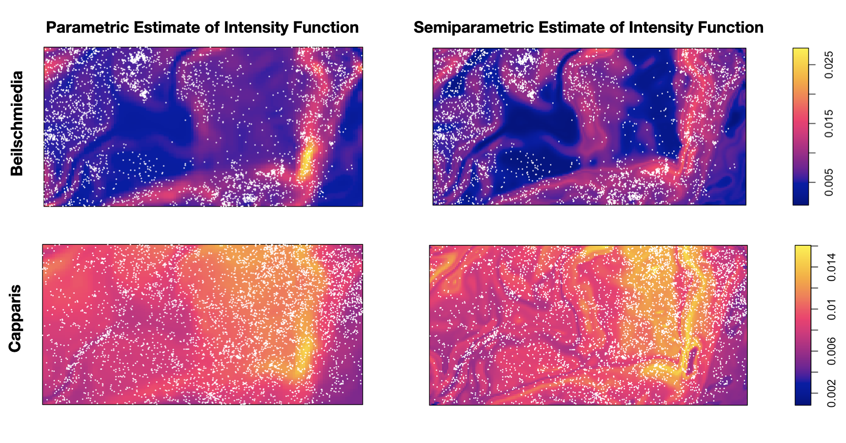
Figure 1: Heat maps of the estimated intensity functions for two different tree species, Beilschmiedia pendula and Capparis frondosa. Each column represents different estimators and each row represents different tree species. The points in each plot are the observed locations of the trees.

For Beilschmiedia pendula, the estimated partial effect of elevation from our estimator is 3.136 (95% CI: (-1.470, 7.741)) whereas the estimate from the parametric approach discussed in Section 5.3 is 2.144 (95% CI: (-2.453, 6.741)). To understand the difference between the two estimates, we plotted the estimated nuisance function from Algorithm 1 and found that there is a non-linear relationship between the gradient and the spatial locations of Beilschmiedia pendula; see Figure 2. From this, we suspect that the inference based on the parametric model may suffer from bias due to model mis-specification of the nuisance parameter. We also remark that the estimated intensity map with our estimator is a better visual fit to the data compared to that from the parametric estimator, especially in the upper left corner of the observation window; see the top row of Figure 1.

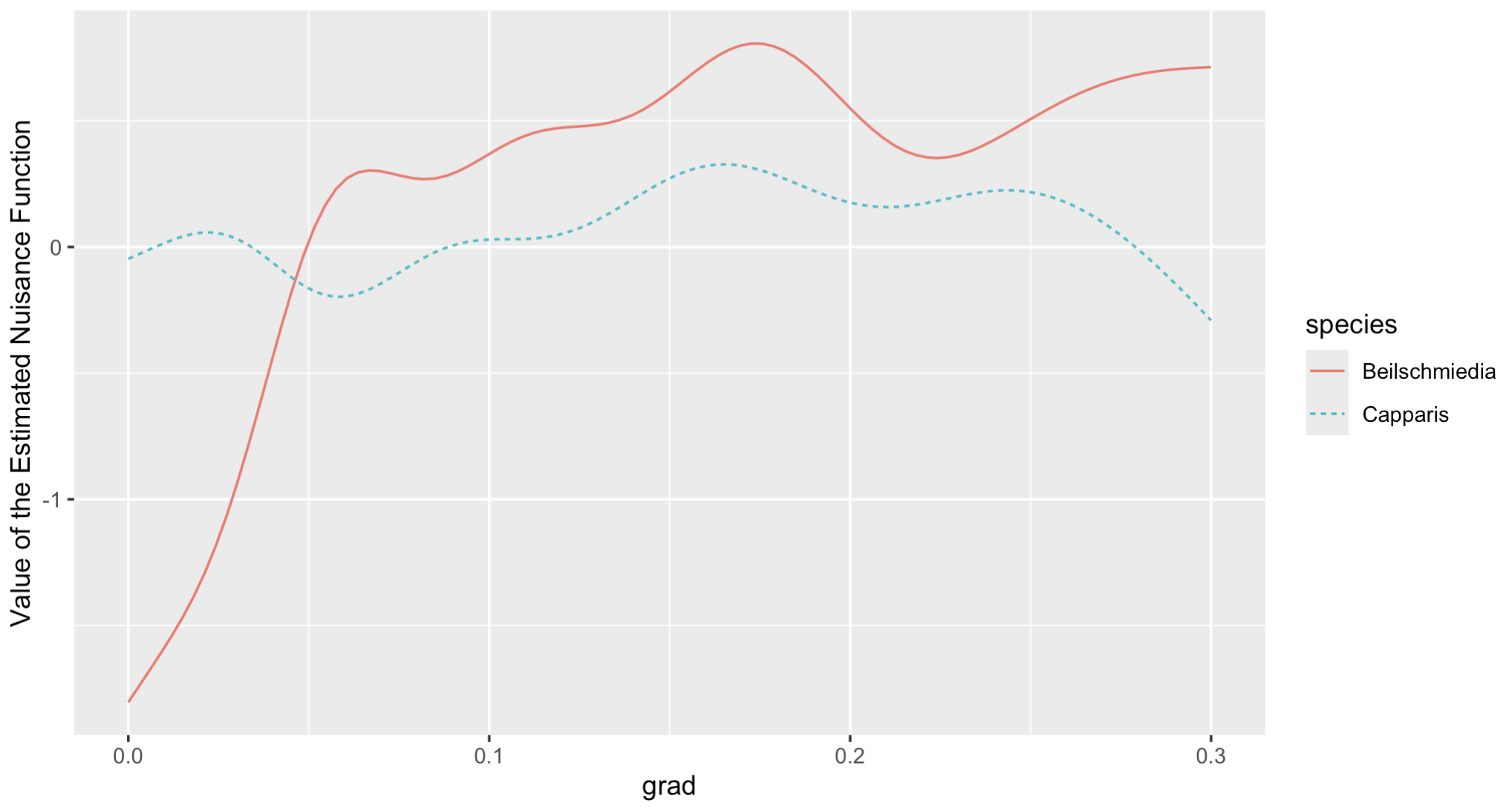
Figure 2: Estimated nuisance function for Beilschmiedia pendula (solid line) and Capparis frondosa (dashed line). grad stands for the gradient, i.e., the nuisance covariate.

For Capparis frondosa, the estimated partial effect of elevation from our estimator is 2.555 (95% CI: (-0.046, 5.151)) whereas the estimate from the parametric approach is 2.692 (95% CI: (0.038, 5.347)). Upon examining the estimated nuisance function, we found that the gradient had a flat, negligible effect on the spatial distribution of Capparis frondosa; see Figure 2. This explains the similarity between our estimator and the parametric estimator for this species. However, visually speaking, the estimated intensity function from our method captures more details in the observation window than that from the parametric estimator, especially in the bottom right of the observation window; see the bottom row of Figure 1. Overall, because our approach makes fewer assumptions about the parametric form of the nuisance covariate, our estimates of the elevation effect are likely more robust than those from the parametric approach.

6 Discussion

The paper studied estimation and inference of semiparametric spatial point processes. We proposed a spatial cross-fitting estimator of the parametric component and proved some favorable properties of the estimator, including consistency and asymptotic Normality. We also proposed a spatial kernel regression, which can achieve the desired rates of convergence for inference. Finally, we generalized the concept of the semiparametric efficiency lower bound in i.i.d. settings to spatial point processes and showed that our estimator can achieve this bound when the process is Poisson. In our simulation study, the proposed estimator is shown to exhibit the asymptotic properties in finite samples.

As laid out in Table 1, there are some remaining challenges when $X$ is not Poisson and the intensity function is not log-linear. We conjecture that establishing asymptotic Normality of $\hat{\boldsymbol{\theta}}$ can be achieved under additional weak dependence restrictions on $X$ and the PCF function. For establishing the efficiency lower bound, we believe that directly utilizing the classical definition of the semiparametric efficiency lower bound (i.e. likelihood-based parametric submodels and the corresponding Cramer-Rao lower bounds) is insufficient. Instead, we believe either restricting the type of estimators (e.g., linear estimators) or a new efficiency criterion is necessary; see Park and Kang, (2022) for a related discussion under network dependence. Overall, we believe our work presents a new approach to study semiparametric point processes and we hope the techniques in the paper is useful to both researchers in point processes and in semiparametric inference.

7 Funding

This work is supported in part by the Groundwater Research and Monitoring Program from the Wisconsin Department of Agriculture, Trade and Consumer Protection.

See pages - of IPP_supplement.pdf

References

- Baddeley et al., (2012) Baddeley, A., Chang, Y.-M., Song, Y., and Turner, R. (2012). Nonparametric estimation of the dependence of a spatial point process on spatial covariates. Statistics and Its Interface, 5(2):221–236.
- Baddeley et al., (2014) Baddeley, A., Coeurjolly, J.-F., Rubak, E., and Waagepetersen, R. (2014). Logistic regression for spatial gibbs point processes. Biometrika, 101(2):377–392.
- Baddeley et al., (2008) Baddeley, A., Møller, J., and Pakes, A. G. (2008). Properties of residuals for spatial point processes. Annals of the Institute of Statistical Mathematics, 60(3):627–649.
- Baddeley et al., (2015) Baddeley, A., Rubak, E., and Turner, R. (2015). Spatial Point Patterns: Methodology and Applications with R. CRC press.
- Baddeley and Turner, (2000) Baddeley, A. and Turner, R. (2000). Practical maximum pseudolikelihood for spatial point patterns: (with discussion). Australian & New Zealand Journal of Statistics, 42(3):283–322.
- Baddeley and Turner, (2005) Baddeley, A. and Turner, R. (2005). Spatstat: an r package for analyzing spatial point patterns. Journal of Statistical Software, 12:1–42.
- Berman and Diggle, (1989) Berman, M. and Diggle, P. (1989). Estimating weighted integrals of the second-order intensity of a spatial point process. Journal of the Royal Statistical Society, Series B (Statistical Methodology), 51(1):81–92.
- Berman and Turner, (1992) Berman, M. and Turner, T. R. (1992). Approximating point process likelihoods with glim. Journal of the Royal Statistical Society, Series C (Applied Statistics), 41(1):31–38.
- Biscio and Lavancier, (2016) Biscio, C. A. and Lavancier, F. (2016). Brillinger mixing of determinantal point processes and statistical applications. Electronic Journal of Statistics, 10:582–607.
- Chernozhukov et al., (2018) Chernozhukov, V., Chetverikov, D., Demirer, M., Duflo, E., Hansen, C., Newey, W., and Robins, J. (2018). Double/debiased machine learning for treatment and structural parameters. The Econometrics Journal, 21(1):C1–C68.
- Chu et al., (2022) Chu, T., Guan, Y., Waagepetersen, R., and Xu, G. (2022). Quasi-likelihood for multivariate spatial point processes with semiparametric intensity functions. Spatial Statistics, 50:100605.
- Condit et al., (1996) Condit, R., Hubbell, S. P., and Foster, R. B. (1996). Changes in tree species abundance in a neotropical forest: impact of climate change. Journal of Tropical Ecology, 12(2):231–256.
- Cronie et al., (2024) Cronie, O., Moradi, M., and Biscio, C. A. (2024). A cross-validation-based statistical theory for point processes. Biometrika, 111(2):625–641.
- Diggle, (1990) Diggle, P. J. (1990). A point process modelling approach to raised incidence of a rare phenomenon in the vicinity of a prespecified point. Journal of the Royal Statistical Society, Series A (Statistics in Society), 153(3):349–362.
- Green and Sibson, (1978) Green, P. J. and Sibson, R. (1978). Computing dirichlet tessellations in the plane. The Computer Journal, 21(2):168–173.
- Guan et al., (2015) Guan, Y., Jalilian, A., and Waagepetersen, R. (2015). Quasi-likelihood for spatial point processes. Journal of the Royal Statistical Society, Series B (Statistical Methodology), 77(3):677–697.
- Guan and Loh, (2007) Guan, Y. and Loh, J. M. (2007). A thinned block bootstrap variance estimation procedure for inhomogeneous spatial point patterns. Journal of the American Statistical Association, 102(480):1377–1386.
- Härdle et al., (2000) Härdle, W., Liang, H., and Gao, J. (2000). Partially Linear Models. Springer Science & Business Media.
- Hessellund et al., (2022) Hessellund, K. B., Xu, G., Guan, Y., and Waagepetersen, R. (2022). Semiparametric multinomial logistic regression for multivariate point pattern data. Journal of the American Statistical Association, 117(539):1500–1515.
- Hubbell, (1983) Hubbell, Stephen P. Foster, R. B. (1983). Diversity of canopy trees in a neotropical forest and implications for conservation. Tropical Rain Forest: Ecology and Management, pages 25–41.
- Jiang et al., (2023) Jiang, Z., Chen, S., and Ding, P. (2023). An instrumental variable method for point processes: generalized wald estimation based on deconvolution. Biometrika, 110(4):989–1008.
- Jones, (1993) Jones, M. C. (1993). Simple boundary correction for kernel density estimation. Statistics and Computing, 3:135–146.
- Li and Racine, (2023) Li, Q. and Racine, J. S. (2023). Nonparametric Econometrics: Theory and Practice. Princeton University Press.
- Møller and Schoenberg, (2010) Møller, J. and Schoenberg, F. P. (2010). Thinning spatial point processes into poisson processes. Advances in Applied Probability, 42(2):347–358.
- Moller and Waagepetersen, (2003) Moller, J. and Waagepetersen, R. P. (2003). Statistical Inference and Simulation for Spatial Point Processes. CRC press.
- Papadogeorgou et al., (2022) Papadogeorgou, G., Imai, K., Lyall, J., and Li, F. (2022). Causal inference with spatio-temporal data: estimating the effects of airstrikes on insurgent violence in iraq. Journal of the Royal Statistical Society, Series B (Statistical Methodology), 84(5):1969–1999.
- Park and Kang, (2022) Park, C. and Kang, H. (2022). Efficient semiparametric estimation of network treatment effects under partial interference. Biometrika, 109(4):1015–1031.
- Racine, (2001) Racine, J. (2001). Bias-corrected kernel regression. Journal of Quantitative Economics, 17(1):25–42.
- Rathbun and Cressie, (1994) Rathbun, S. L. and Cressie, N. (1994). Asymptotic properties of estimators for the parameters of spatial inhomogeneous poisson point processes. Advances in Applied Probability, 26(1):122–154.
- Robinson, (1988) Robinson, P. M. (1988). Root-n-consistent semiparametric regression. Econometrica: Journal of the Econometric Society, pages 931–954.
- Schoenberg, (2005) Schoenberg, F. P. (2005). Consistent parametric estimation of the intensity of a spatial–temporal point process. Journal of Statistical Planning and Inference, 128(1):79–93.
- Severini and Staniswalis, (1994) Severini, T. A. and Staniswalis, J. G. (1994). Quasi-likelihood estimation in semiparametric models. Journal of the American Statistical Association, 89(426):501–511.
- Severini and Wong, (1992) Severini, T. A. and Wong, W. H. (1992). Profile likelihood and conditionally parametric models. The Annals of Statistics, pages 1768–1802.
- Tang and Li, (2023) Tang, X. and Li, L. (2023). Multivariate temporal point process regression. Journal of the American Statistical Association, 118(542):830–845.
- van der Vaart and Wellner, (1996) van der Vaart, A. and Wellner, J. A. (1996). Weak Convergence and Empirical Processes With Applications to Statistics. Springer.
- van Lieshout, (2012) van Lieshout, M.-C. N. (2012). On estimation of the intensity function of a point process. Methodology and Computing in Applied Probability, 14:567–578.
- Waagepetersen and Guan, (2009) Waagepetersen, R. and Guan, Y. (2009). Two-step estimation for inhomogeneous spatial point processes. Journal of the Royal Statistical Society, Series B (Statistical Methodology), 71(3):685–702.
- Watson, (1964) Watson, G. S. (1964). Smooth regression analysis. Sankhyā: The Indian Journal of Statistics, Series A, 26(4):359–372.
- Wood, (2001) Wood, S. N. (2001). mgcv: Gams and generalized ridge regression for r. R news, 1(2):20–25.