HyperBlocker: Accelerating Rule-based Blocking in Entity Resolution using GPUs

Abstract.

This paper studies rule-based blocking in Entity Resolution (ER). We propose $\mathsf{HyperBlocker}$, a GPU-accelerated system for blocking in ER. As opposed to previous blocking algorithms and parallel blocking solvers, $\mathsf{HyperBlocker}$ employs a pipelined architecture to overlap data transfer and GPU operations. It generates a data-aware and rule-aware execution plan on CPUs, for specifying how rules are evaluated, and develops a number of hardware-aware optimizations to achieve massive parallelism on GPUs. Using real-life datasets, we show that $\mathsf{HyperBlocker}$ is at least 6.8$\times$ and 9.1$\times$ faster than prior CPU-powered distributed systems and GPU-based ER solvers, respectively. Better still, by combining $\mathsf{HyperBlocker}$ with the state-of-the-art ER matcher, we can speed up the overall ER process by at least 30% with comparable accuracy.

PVLDB Artifact Availability:
The source code, data, or other artifacts have been made available at %leave␣empty␣if␣no␣availability␣url␣should␣be␣set%\newcommand\vldbavailabilityurl{}https://github.com/SICS-Fundamental-Research-Center/HyperBlocker.

1. Introduction

Entity resolution (ER), also known as record linkage, data deduplication, merge/purge and record matching, is to identify tuples that refer to the same real-world entity. It is a routine operation in many data cleaning and integration tasks, such as detecting duplicate commodities (Gao et al., 2015) and finding duplicate customers (Deng et al., 2022).

Recently, with the rising popularity of deep learning (DL) models, research efforts have been made to apply DL techniques to ER. Although these DL-based approaches have shown impressive accuracy, they also come with high training/inference costs, due to the large number of parameters. Despite the effort to reduce parameters, the growth in the size of DL models is still an inevitable trend, leading to the increasing time for making matching decisions.

In the worst case, ER solutions have to spend quadratic time examining all pairs of tuples. As reported by Thomson Reuters, an ER project can take 3-6 months, mainly due to the scale of data (Chu et al., 2016). To accelerate, most ER solutions divide ER into two phases: (a) a blocking phase, where a blocker discards unqualified pairs that are guaranteed to refer to distinct entities, and (b) a matching phase, where a matcher compares the remaining pairs to finally decide whether they are matched, i.e., refer to the same entity. The blocking phase is particularly useful when dealing with large data and “is the crucial part of ER with respect to time efficiency and scalability” (Papadakis et al., 2020).

To cope with the volume of big data, considerable research has been conducted on blocking techniques. As surveyed in (Li et al., 2020b; Papadakis et al., 2020), we can divide blocking methods into rule-based (Kolb et al., 2012a; Chu et al., 2016; Isele et al., 2011; Papadakis et al., 2011; Gu and Baxter, 2004) or DL-based (Ebraheem et al., 2018; Thirumuruganathan et al., 2021; Zhang et al., 2020; Javdani et al., 2019), both have their strengths and limitations.

DL-based blocking methods typically utilize pre-trained DL models to generate embeddings for tuples and discard tuple pairs with low similarity scores. While DL-based blocking can enhance ER by parallelizing computation and leveraging GPU acceleration (Johnson et al., 2021), it often comes with long runtime and high memory costs. To justify this, we conducted a detailed analysis on $\mathsf{DeepBlocker}$ (Thirumuruganathan et al., 2021), the state-of-the-art (SOTA) DL-based blocker in Figure 1. We picked a rule-based blocker (a prototype of our method) with comparable accuracy with $\mathsf{DeepBlocker}$ and compared their runtime and memory. The evaluation was conducted on a machine equipped with V100 GPUs using the Songs dataset (Mudgal et al., 2018), varying the number of tuples. When running on one GPU, the runtime of $\mathsf{DeepBlocker}$ increases substantially when the number of tuples exceeds 40k. Worse still, it consumes excessive memory due to the large embeddings and intermediate results during similarity computation. Although the runtime of $\mathsf{DeepBlocker}$ can be reduced by using more GPUs, the issue remains, e.g., even with four GPUs in Figure 1(a), $\mathsf{DeepBlocker}$ is still slower than the rule-based blocker that runs on one GPU.

In contrast, rule-based blocking methods demonstrate potential for achieving scalability by leveraging multiple blocking rules. Each rule employs various comparisons with logical operators such as AND, OR, and NOT to discard unqualified tuple pairs. For instance, a blocking rule for books may state “If titles match and the number of pages match, then the two books match” (Konda et al., 2016). We refer to the comparisons in this rule as equality comparisons, as they require exact equality. Another example, referred to as similarity comparisons, is presented in (Papadakis et al., 2011), which adopts the Jaccard similarity to determine whether a pair of tuples requires further matching. Rule-based approaches complement DL-based approaches by providing flexibility, explainability, and scalability in the blocking process (Barlaug, 2023). Moreover, by incorporating domain knowledge into blocking rules, these approaches can readily adapt to different domains.

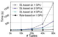
(a) Execution time

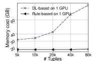
(b) Memory cost on a single GPU

Figure 1. DL-based blocking vs. rule-based blocking

Example 1.

As a critical step for data consistency, an e-commerce company (e.g., Amazon (ama, 2023)) conducts ER for products, to enhance operations for e.g., product listings and inventory management.

To identify duplicate products, the blocking rule $\varphi_{1}$ may fit.

$\varphi_{1}$: Two products are potentially matched if (a) they have same color and price, (b) they are sold at same store, (c) their names are similar.

Here $\varphi_{1}$ is a conjunction of attribute-wise comparisons, where both equality (parts (a) and (b)) and similarity comparisons (part (c)) are involved. In Section 2, we will formally define $\varphi_{1}$.

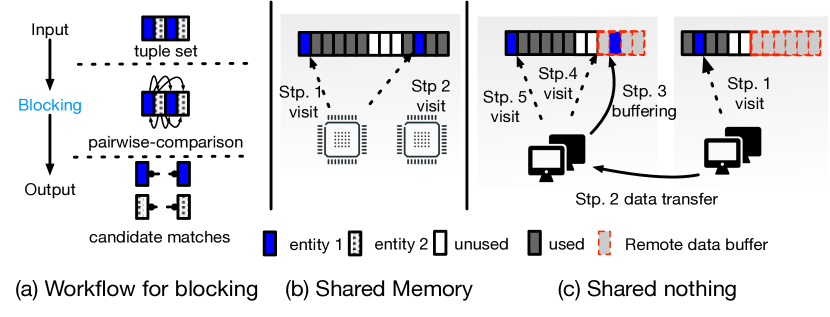
Figure 2. Shared memory vs shared nothing architectures

Rule-based blocking in ER has attracted a lot of attention (surveyed in (Li et al., 2020b; Papadakis et al., 2020)). Unfortunately, most of existing rule-based blockers are designed for CPU-based (shared nothing) architectures, leading to unsatisfactory performance. Specifically, a blocker typically conducts pairwise comparisons on all pairs of tuples to obtain candidate matches (Figure 2(a)). In a shared-nothing architecture, data is partitioned and spread across a set of processing units. Each unit independently blocks data using its local memory, which may lead to skewed partitions/computations and rising communication costs, e.g., in Figure 2(c), the first unit is assigned more tuples than the second one and worse still, two tuples that both refer to entity 1 are distributed to different partitions. To avoid missing this match, the second unit has to visit its local memory (Stp. 1) and transfer its data to the first unit (Stp. 2). Then the first unit buffers the data (Stp. 3) and finally, conducts comparison locally (Stp. 4 & 5). The shared memory architecture (Figure 2(b)) is the opposite: all data is accessible from all processing units, allowing for efficient data sharing, collaboration between processing units and dynamic workload scheduling, e.g., the two tuples referred to entity 1 can be directly accessed by both units in Figure 2(b) (Stp. 1 & 2). GPUs are typically based on shared memory architectures, offering promising opportunities to achieve blocking parallelism. However, unlike DL-based blocking approaches, few rule-based methods support the massive parallelism offered by GPUs, despite their greater potential (see Figure 1).

To make practical use of rule-based blocking, several questions have to be answered. Can we parallelize it under a share memory architecture, utilizing massive parallelism of a GPU? Can we explore characteristics of GPUs and CPUs, to effectively collaborate them?

HyperBlocker. To answer these, we develop $\mathsf{HyperBlocker}$, a GPU-accelerated system for rule-based blocking in Entity Resolution. As proof of concept, we adopt matching dependencies ($\mathsf{MDs}$) (Fan et al., 2011) for rule-based blocking. As a class of rules developed for record matching, $\mathsf{MDs}$ are defined as a conjunction of (similarity) predicates and support both equality and similarity comparisons. Compared with prior works, $\mathsf{HyperBlocker}$ has the following unique features.

(1) A pipelined architecture. $\mathsf{HyperBlocker}$ adopts an architecture that pipelines the memory access from/to CPUs for data transfer, and operations on GPUs for rule-based blocking. In this way, the data transfer and the computation on GPUs can be overlapped.

(2) Execution plan on CPUs. To effectively filter unqualified pairs, blocking must be optimized for the underlying data (resp. blocking rules) for both equality and similarity comparisons; in this case, we say that the blocking is data-aware (resp. rule-aware). To our knowledge, prior methods either fail to consider data/rule-awareness or cannot handle arbitrary comparisons well. $\mathsf{HyperBlocker}$ designs an execution plan generator to warrant efficient rule-based blocking.

(3) Hardware-aware parallelism on GPUs. Due to different characteristics of CPUs and GPUs, a naive approach that applies existing CPU-based blocking on GPUs makes substantial processing capacity untapped. We develop a variety of GPU-based parallelism strategies, designated for rule-based blocking, by exploiting the hardware characteristics of GPUs, to achieve massive parallelism.

(4) Multi-GPUs collaboration. It is already hard to offload tasks on CPUs. This problem is even exacerbated under multi-GPUs, due to the complexities of task decomposition, (inter-GPU) resource management, and workload balancing. $\mathsf{HyperBlocker}$ provides effective partitioning and scheduling strategies to scale with multiple GPUs.

Contribution & organization. After reviewing background in Section 2, we present $\mathsf{HyperBlocker}$ as follows: (1) its unique architecture and system overview (Section 3); (2) the rule/data-aware execution plan generator (Section 4); (3) the hardware-aware parallelism and the task scheduling strategy across GPUs (Section 5); and (4) an experimental study (Section 6). Section 7 presents related work.

Using real-life datasets, we find the following: (a) $\mathsf{HyperBlocker}$ speedups prior distributed blocking systems and GPU baselines by at least 6.8$\times$ and 9.1$\times$, respectively. (b) Combining $\mathsf{HyperBlocker}$ with the SOTA ER matcher saves at least 30% time with comprable accuracy. (c) $\mathsf{HyperBlocker}$ is scalable, e.g., it can process 36M tuples in 1604s. (d) While promising, DL-based blocking methods are not always the best. By carefully optimizing rule-based blocking on GPUs, we share valuable lessons/insights about when rule-based approaches can beat the DL-based ones and vice versa.

Table 1. A relation $D$ of schema $\mathsf{Products}$, where the dash (“-”) denotes a missing value.

$\mathsf{eid}$	$\mathsf{pno}$	$\mathsf{pname}$	$\mathsf{price}$	$\mathsf{sname}$	$\mathsf{description}$	$\mathsf{color}$	$\mathsf{saddress}$
$e_{1}$	$t_{1}$	Apple Mac Air	$909	Comp. World	Apple MacBook Air (13-inch, 8GB RAM, 256GB SSD)	Gray	9 Barton Grove, McCulloughmouth
$e_{2}$	$t_{2}$	ThinkPad	-	Smith’s Tech	ThinkPad E15, 15.6-inch full HD IPS display, Intel Core i5-1235U processor, (16GB) RAM — 512GB PCIe SSD)	Gray	Seg Plaza, Hua qiang North Road
$e_{2}$	$t_{3}$	ThinkPad	$849	Smith’s Tech	Lenovo E15 Business ThinkPad, 15.6-inch full HD IPS display, 12 generation Intel Core i5, 16GB RAM, 512GB SSD	Gray	Seg Plaza, Hua qiang North Road
$e_{1}$	$t_{4}$	MacBook Air	$909	Comp. World	Apple 2022 MacBook Air M2 chip 13-inch,8 GB RAM,256 GB SSD storage gray	Gray	-
$e_{1}$	$t_{5}$	MacBook Air	$909	Comp. World	-	Gray	Barton Grove, McCulloughmouth

2. Preliminaries

We first review notations (more in (ful, 2024)) for ER, blocking, and GPUs.

Relations. Consider a schema $R=({\mathsf{eid}},A_{1},\dotsc,\allowbreak A_{n})$, where $A_{i}$ is an attribute ($i\in[1,n]$), and $\mathsf{eid}$ is an entity id, such that each tuple of $R$ represents an entity. A relation $D$ of $R$ is a set of tuples of schema $R$.

Entity resolution (ER). Given a relation $D$, ER is to identify all tuple pairs in $D$ that refer to the same real-life entity. It returns a set of tuple pairs $(t_{1},t_{2})$ of $D$ that are identified as matches. If $t_{1}$ does not match $t_{2}$, $(t_{1},t_{2})$ is referred to as a mismatch.

Most existing methods typically conduct ER in three steps:

(1) Data partitioning. The tuples in relation $D$ are divided into multiple data partitions, namely $P_{1},P_{2},...,P_{m}$, so that tuples of similar entities tend to be put into the same data partition.

(2) Blocking. Each tuple pair $(t_{1},t_{2})$ from a partition $P$ is a potential match that requires further verification. To reduce cost, a blocking method ${\mathcal{A}}_{\mathsf{block}}$ (i.e., blocker) is often adopted to filter out those pairs that are definitely mismatches efficiently, instead of directly verifying every tuple pair. Denote the set of remaining pairs obtained from $P$ by ${\mathsf{Ca}}(P)=\{(t_{1},t_{2})\in P\times P\mid(t_{1},t_{2})\text{ is not filtered by }{\mathcal{A}}_{\mathsf{block}}\}$.

(3) Matching. For each pair in ${\mathsf{Ca}}(P)$, an accurate (but expensive) matcher is applied, to make final decisions of matches/mismatches.

Our scope: blocking. Note that in some works, both steps (1) and (2) are called blocking. To avoid ambiguity, we follow (Thirumuruganathan et al., 2021) and distinguish partitioning from blocking. We mainly focus on blocking, i.e.,

• Input: A relation $D$ of the tuples of schema $R$, where the tuples in $D$ are divided into $m$ partitions $P_{1},\ldots,P_{m}$.

• Output: The set ${\mathsf{Ca}}(P_{i})$ of candidate tuple pairs on each $P_{i}$.

Although our work can be applied on data partitions generated by any existing method, we optimize over multiple data partitions, by exploiting designated GPU acceleration techniques (Section 5.3).

While blocking focuses more on efficiency and matching focuses more on accuracy, they can be used without each other, e.g., one can directly employ rules (Fan et al., 2011) for ER or apply an ER matcher (Li et al., 2020a) on the Cartesian product of the entire partition. When blocking is used alone on a given partition $P$, all tuple pairs in ${\mathsf{Ca}}(P)$ are identified as matches. In Section 6, we will test $\mathsf{HyperBlocker}$ with or without a matcher, to elaborate the trade-off between efficiency and accuracy.

Rule-based blocking. We study rule-based blocking in this paper, due to its efficiency and explainability remarked earlier. We review a class of matching dependencies ($\mathsf{MDs}$), originally proposed in (Fan et al., 2011).

Predicates. Predicates over schema $R$ are defined as follows:

$$p::=t.A=c\ |\ t.A=s.B\ |\ t.A\approx s.B\vspace{-0.7ex}$$

where $t$ and $s$ are tuple variables denoting tuples of $R$, $A$ and $B$ are attributes of $R$ and $c$ is a constant; $t.A=s.B$ and $t.A=c$ compare the equality on compatible values, e.g., $t.{\mathsf{eid}}=s.{\mathsf{eid}}$ says that $(t,s)$ is a potential match; $t.A\approx s.B$ compares the similarity of $t.A$ and $s.B$. Here any similarity measure, symmetric or asymmetric, can be used as $\approx$, e.g., edit distance or KL divergence, such that $t.A\approx s.B$ is true if $t.A$ and $s.B$ are “similar” enough w.r.t. a threshold. Sophisticated similarity measures like ML models can also be used as in (Fan et al., 2022; Bao et al., 2024).

Rules. A (bi-variable) matching dependency ($\mathsf{MD}$) over $R$ is:

$$\varphi=X\rightarrow l,\vspace{-0.7ex}$$

where $X$ is a conjunction of predicates over $R$ with two tuple variables $t$ and $s$, and $l$ is $t.{\mathsf{eid}}=s.{\mathsf{eid}}$. We refer to $X$ as the precondition of $\varphi$, and $l$ as the consequence of $\varphi$, respectively.

Example 1.

Consider a (simplified) e-commence database with self-explained schema $\mathsf{Products}$ ($\mathsf{eid}$, $\mathsf{pno}$, $\mathsf{pname}$, $\mathsf{price}$, $\mathsf{sname}$ (store name), $\mathsf{description}$, $\mathsf{color}$, $\mathsf{saddress}$ (store address)). Below are some examples $\mathsf{MDs}$, where the rule in Example 1 is written as $\varphi_{1}$.

(1) $\varphi_{1}:t.{\mathsf{color}}=s.{\mathsf{color}}\land t.{\mathsf{price}}=s.{\mathsf{price}}\land t.{\mathsf{sname}}=s.{\mathsf{sname}}\allowbreak\land t.{\mathsf{pname}}\approx_{\mathsf{ED}}s.{\mathsf{pname}}\to t.{\mathsf{eid}}=s.{\mathsf{eid}}$, where $\approx_{\mathsf{ED}}$ measures the edit distance. As stated before, $\varphi_{1}$ identifies two products, by their colors, prices, product names and the stores sold.

(2) $\varphi_{2}:t.{\mathsf{sname}}=s.{\mathsf{sname}}\land t.{\mathsf{description}}\approx_{\mathsf{JD}}s.{\mathsf{description}}\to t.{\mathsf{eid}}\allowbreak=s.{\mathsf{eid}}$, where $\approx_{\mathsf{JD}}$ measures the Jaccard distance. The $\mathsf{MD}$ says that if two products are sold in the store and have a similar description, then they are identified as a potential match.

(3) $\varphi_{3}:t.{\mathsf{saddress}}\approx_{\mathsf{ED}}s.{\mathsf{saddress}}\land t.{\mathsf{description}}\approx_{\mathsf{JD}}s.{\mathsf{description}}\allowbreak\to t.{\mathsf{eid}}=s.{\mathsf{eid}}$. It gives another condition for identifying two products, i.e., the two products with similar descriptions are sold from stores with similar addresses are potentially matched.

Semantics. A valuation of tuple variables of an $\mathsf{MD}$ $\varphi$ in $D$, or simply a valuation of $\varphi$, is a mapping $h$ that instantiates the two variables $t$ and $s$ with tuples in $D$. A valuation $h$ satisfies a predicate $p$ over $R$, written as $h\models p$, if the following is satisfied: (1) if $p$ is $t.A=c$ or $t.A=s.B$, then it is interpreted as in tuple relational calculus following the standard semantics of first-order logic (Abiteboul et al., 1995); and (2) if $p$ is $t.A\approx s.B$, then $h(t).A\approx h(s).B$ returns true. Given a conjunction $X$ of predicates, we say $h\models X$ if for all predicates $p$ in $X$, $h\models p$.

Blocking. Rule-based blocking employs a set $\Delta$ of $\mathsf{MDs}$. Given a partition $P$, a pair $(t_{1},t_{2})\in P\times P$ is in ${\mathsf{Ca}}(P)$ iff there exists an $\mathsf{MD}$ $\varphi$ in $\Delta$ such that the valuation $h(t_{1},t_{2})$ of $\varphi$ that instantiates variables $t$ and $s$ with tuples $t_{1}$ and $t_{2}$ satisfies the precondition of $\varphi$; we call such $\varphi$ as a witness at $(t_{1},t_{2})$, since it indicates that $(t_{1},t_{2})$ is a potential match. Otherwise, $(t_{1},t_{2})$ will be filtered. Since a precondition is a conjunction of predicates, rule-based blocking is in Disjunctive normal form (DNF), i.e., it is to evaluate a disjunction of conjunctions.

Example 2.

Continuing with Example 1, consider $D$ in Table 1 and $h(t_{1},t_{4})$ that instantiates variables $t$ and $s$ with tuples $t_{1}$ and $t_{4}$ in $D$. Since $h(t_{1},t_{4})$ satisfies the precondition of $\varphi_{1}$, $\varphi_{1}$ is a witness at $(t_{1},t_{4})$. Similarly, one can verify that $\varphi_{1}$ is not a witness at $(t_{2},t_{3})$.

Discovery of $\mathsf{MDs}$. $\mathsf{MDs}$ can be considered as a special case of entity enhancing rules ($\mathsf{REEs}$) (Fan et al., 2022, 2023). We can readily apply the discovery algorithms for $\mathsf{REEs}$, e.g., (Fan et al., 2022, 2023), to discover $\mathsf{MDs}$ (details omitted).

GPU hardware. As general processors for high-performance computation, GPUs offer the following benefits compared with CPUs.

First, GPUs provide massive parallelism by programming with CUDA (Compute Unified Device Architecture) (Lippuner, 2019). A GPU has multiple SMs (Streaming Multiprocessors), where each SM accommodates multiple processing units. e.g., V100 has 80 SMs, each with 64 CUDA cores. SMs handle the parallel execution of CUDA cores. In CUDA programming, CUDA cores are conceptually organized into TBs (Thread Blocks) and physically grouped into thread warps, each comprising subgroups of 32 threads. This hierarchical organization allows thousands of threads running simultaneously on GPUs.

Second, GPUs utilize the DMA (Direct Memory Access) technology, which enables direct data transfer between GPU memory and system memory. This not only reduces CPU overhead but also allows the GPU to handle multiple data streams simultaneously. However, the number of PCIe lanes determines the maximum number of streams that can transfer data simultaneously (e.g., 16 PCIe lanes for V100). When multiple partitions perform data transfers over a PCIe lane, only one can utilize the lane at a time.

Third, GPUs adopt SIMT (Single Instruction, Multiple Threads) execution, where each SIMT lane is an individual unit that is responsible for executing a thread under a single instruction. Thread divergence can adversely affect the performance and it typically occurs in conditional statements (e.g., if-else), where some lanes take one execution path while the others take a different path. However, GPUs must execute different execution paths sequentially, rather than in parallel, resulting in underutilization of GPU resources.

3. HyperBlocker: System Overview

In this section, we present the overview of $\mathsf{HyperBlocker}$, a GPU-accelerated system for rule-based blocking that optimizes the efficiency by considering rules, underlying data, and hardware simultaneously. In the literature, GPUs and CPUs are usually referred to as devices and hosts, respectively. We also follow this terminology.

Challenges. Existing parallel blocking methods typically rely on multiple CPU-powered machines under the shared nothing architecture, to achieve data partition-based parallelism. They reduce the runtime by using more machines, which, however, is not always feasible due to the increasing communication cost (see Section 1).

In light of these, $\mathsf{HyperBlocker}$ focuses on parallel blocking under a shared memory architecture; this introduces new challenges.

(1) Execution plan for efficient blocking. The efficiency of blocking depends heavily on how much/fast we can filter mismatches. Therefore, a good execution plan that specifies how rules are evaluated is crucial. However, most existing blocking optimizers fail to consider the properties of rules/data for blocking and even the optimizers of popular DBMS (e.g., PostgreSQL (pos, 2024)) may not work well when handling similarity comparisons and evaluating queries in DNF (see Section 4). This motivates us to design a different plan generator.

(2) Hardware-aware parallelism. When GPUs are involved, those CPU-based techniques adopted in existing solvers no longer suffice, since GPUs have radically different characteristics (Section 2). Novel GPU-based parallelism for blocking is required to improve GPU utilization, e.g., by reducing thread wait stalls and thread divergence.

(3) Multi-GPUs collaboration. Existing parallel blocking solvers focus on minimizing the communication cost across all workers (Chu et al., 2016; Deng et al., 2022). However, this objective no longer applies in multi-GPUs scenarios, where unique challenges such as task decomposition, (inter-GPU) resource management and task scheduling arise.

Novelty. The ultimate goal of $\mathsf{HyperBlocker}$ is to generate the set ${\mathsf{Ca}}(P)$ of potential matches on each data partition $P$. To achieve this, we implement three novel components as follows:

(1) Execution plan generator (EPG) (Section 4). We develop a generator to generate data-aware and rule-aware execution plans, which support arbitrary comparisons and work well with DNF evaluation. Here we say an execution plan is data-aware, since it considers the distribution of data to decide which predicates are evaluated first; similarly, it is rule-aware, since it is optimized for underlying rules.

(2) Parallelism optimizer (Section 5). We implement a specialized optimizer that exploits the hierarchical structure of GPUs, to optimize the power of GPUs by utilizing thread blocks (TBs) and warps. With this optimizer, blocking can be effectively parallelized on GPUs.

(3) Resource scheduler (Section 5). To achieve optimal performance over multiple GPUs, a partitioning strategy and a resource scheduler are developed to manage the resources, and balance the workload across multiple GPUs, minimizing idle time and resource waste.

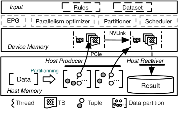
Figure 3. The pipelined architecture of $\mathsf{HyperBlocker}$

Architecture. The architecture of $\mathsf{HyperBlocker}$ is shown in Figure 3. Taken a relation $D$ of tuples and a set $\Delta$ of $\mathsf{MDs}$ discovered offline as input, $\mathsf{HyperBlocker}$ divides the tuples in $D$ into $m$ disjoint partitions and asynchronously processes these data partitions in a pipelined manner, so that the execution at devices and the data transfer can be overlapped. Such architecture helps to mitigate the excessive I/O costs, reduce idle time, and improve hardware utilization.

Workflow. More specifically, $\mathsf{HyperBlocker}$ works in five steps:

(1) Data partitioning. $\mathsf{HyperBlocker}$ divides the tuples in $D$ into $m$ partitions, to allow parallel processing asynchronously.

(2) Execution plan generation. Given the set $\Delta$ of $\mathsf{MDs}$ discovered offline, an execution plan that specifies in what order the rules (and the predicates in rules) should be evaluated is generated at the host.

(3) Host scheduling. The blocking on each partition forms a computational task and the host dynamically assigns tasks to the queue(s) of available devices without interrupting their ongoing execution, minimizing the idle time of devices and improving resource utilization.

(4) Device execution. When a device receives the task assigned, it conducts the rule-based blocking on the corresponding data partition, following the execution plan generated in Step (2).

(5) Result retrieval. Once a task is completed on a device, the host will pull/collect the result (i.e., ${\mathsf{Ca}}(P)$) from the device.

To facilitate processing, $\mathsf{HyperBlocker}$ has two additional components: $\mathsf{HostProducer}$ and $\mathsf{HostReceiver}$, where the former manages Steps (1), (2), and (3) and the latter handles Step (5). Steps (3) (4) (5) in $\mathsf{HyperBlocker}$ work asynchronously in a pipeline manner.

4. EPG: Execution Plan Generator

Given the set $\Delta$ of $\mathsf{MDs}$ and a partition $P$ of $D$, a naive approach to compute ${\mathsf{Ca}}(P)$ is to evaluate each $\mathsf{MD}$ in $\Delta$ for all pairs in $P$. That is, to decide whether $(t_{1},t_{2})$ is in ${\mathsf{Ca}}(P)$, we perform $O(\sum_{\varphi\in\Delta}|\varphi|)$ predicate evaluation, where $|\varphi|$ is the number of predicates in $\varphi$. Worse still, there are $O(|\Delta|!|\varphi|!)$ possible ways to evaluate all $\mathsf{MDs}$ in $\Delta$, since both $\mathsf{MDs}$ in $\Delta$ and predicates in each $\varphi$ can be evaluated in arbitrary orders. However, not all orders are equally efficient.

Example 1.

In Example 2, $\varphi_{1}$ is a witness at $(t_{1},t_{4})$ while $\varphi_{3}$ is not. If we first evaluate $\varphi_{1}$ for $(t_{1},t_{4})$, $(t_{1},t_{4})$ is identified as a potential match and there is no need to evaluate $\varphi_{3}$. Moreover, when evaluating $\varphi_{1}$ for another pair $(t_{2},t_{3})$, we can conclude that $\varphi_{1}$ is not a witness at $(t_{2},t_{3})$, as soon as we find $h(t_{2},t_{3})\not\models t.{\mathsf{price}}=s.{\mathsf{price}}$.

Challenges. Given the huge number of possible evaluation orders, it is non-trivial to define a good one, for three reasons:

(1) Rule priority. Recall that rule-based blocking is in DNF, i.e., as long as there exists a witness at $(t_{1},t_{2})$, $(t_{1},t_{2})$ will be considered as a potential match. This motivates us to prioritize the rules in $\Delta$ so that promising ones can be evaluated early; once a witness is found, the evaluation of the remaining rules can be skipped.

(2) Reusing computation. $\mathsf{MDs}$ may have common predicates. To avoid evaluating a predicate repeatedly, we reuse previous results whenever possible, e.g., given $(t_{1},t_{2})$, $\varphi_{1}:p\land X_{1}\rightarrow l$ and $\varphi_{2}:p\land X_{2}\allowbreak\rightarrow l$, if $\varphi_{1}$ is not a witness at $(t_{1},t_{2})$ since $h(t_{1},t_{2})\not\models p$, neither is $\varphi_{2}$.

(3) Predicate ordering. Given $(t_{1},t_{2})$ and $\varphi:X\rightarrow l$, $\varphi$ is not a witness at $(t_{1},t_{2})$ if we find the first $p$ in $X$ such that $h(t_{1},t_{2})\not\models p$. However, to decide which predicate is evaluated first, we have to consider both its evaluation cost and its effectiveness/selectivity.

As remarked in (Fan et al., 2021; Bao et al., 2024), blocking with a set of $\mathsf{MDs}$ can be implemented in a single DNF SQL query (i.e., an OR of ANDs), where similarity predicates in $\mathsf{MDs}$ are re-written as user-defined functions (UFDs). In light of this, one may want to adopt the optimizers of existing DBMS to tackle rule-based blocking, which, however, may not work well, for several reasons. (a) The mixture of relational operators and UDFs poses serious challenges to an optimizer (Rheinländer et al., 2017). It may lack “the information needed to decide whether they can be reordered with relational operators and other UDFs” (Hueske et al., 2013) and worse still, it is hard to accurately estimate the runtime performance of UDFs (Rheinländer et al., 2017). (b) Using OR operators in WHERE clauses can be inefficient, since it can force the database to perform a full table scan to find matching tuples (bad, 2024). (c) Similar to (Li et al., 2023), if a tuple pair fails to satisfy prior predicates in a blocking rule, the remaining evaluation of this rule can be bypassed directly. While this is undeniably obvious, “many approaches have not leveraged it effectively” (Li et al., 2023).

To justify, we tested $\mathsf{PostgreSQL}$ (pos, 2024), a popular DBMS, on different queries, by (a) specifying similarity predicates in different orders and (b) evaluating SQLs with or without OR operators (see details in (ful, 2024)). An in-depth analysis using $\mathsf{PostgreSQL}$’s EXPLAIN feature reveals the following: (a) Although $\mathsf{PostgreSQL}$ may prioritize equality, it does not optimize the order of similarity predicates well, e.g., it evaluates similarity predicates simply as specified in the SQLs, leading to 20% slowdown on average. (b) When handling OR operators, $\mathsf{PostgreSQL}$ may perform sequential scans with nested loops, without utilizing the hash index. These findings highlight the needs of designated optimization for rule-based blocking, where we have to handle similarity comparisons and DNF evaluation efficiently.

Novelty. In light of these, EPG in $\mathsf{HyperBlocker}$ gives a lightweight solution, by generating an execution plan to make the overall evaluation cost of $\Delta$ as small as possible. Its novelty includes (a) a new notion of execution tree that works no matter what types of comparisons are used, (b) a rule-aware scoring strategy, to decide which $\mathsf{MDs}$ in $\Delta$ are evaluated first, and (c) a data-aware predicate ordering scheme, to strike for a balance between cost and effectiveness.

Below we first give the formal definition of execution plans and then show how EPG generates a good execution plan.

4.1. Execution plan

An execution plan specifies how rules and predicates in $\Delta$ are evaluated. Although an execution plan can be represented in different ways, we represent it as an execution tree, denoted by ${\mathcal{T}}$ in this paper for its conciseness and simplicity (an example is given in Figure 4, to be explained in more detail later). (1) A node in ${\mathcal{T}}$ is denoted by $N$, where the root is denoted by $N_{0}$. (2) A path $\rho$ from the root is a list $\rho=(N_{0},N_{1},\ldots,N_{L})$ such that $(N_{i-1},N_{i})$ is an edge of ${\mathcal{T}}$ for $i\in[1,L]$; the length of $\rho$ is $L$, i.e., the number of edges on $\rho$. (3) We refer to $N_{2}$ as a child node of $N_{1}$ if $(N_{1},N_{2})$ is an edge in ${\mathcal{T}}$, and as a descendant of $N_{1}$ if there exists a path from $N_{1}$ to $N_{2}$; conversely, we refer to $N_{1}$ as a parent node (resp. predecessor) of $N_{2}$. (4) Each edge $e$ represents a predicate $p$ and is associated with a score, denoted by ${\mathsf{score}}(e)$, indicating the priority of $e$. (5) A node is called a leaf if it has no children and ${\mathcal{T}}$ has $|\Delta|$ leaves, where each leaf is associated with a rule $\varphi:X\rightarrow l$ in $\Delta$; the length of the path from the root to the leaf is $|X|$ (i.e., the number of predicates in $X$) and for each predicate in $X$, it appears exactly once in an edge on the path. (6) The leaves of two $\mathsf{MDs}$ may have common predecessors, in addition to the root; intuitively, this means that the $\mathsf{MDs}$ have common predicates. With a slight abuse of notation, we also denote an execution plan by ${\mathcal{T}}$.

Evaluating an execution plan. For each pair $(t_{1},t_{2})$, it is evaluated by exploring ${\mathcal{T}}$ via depth-first search (DFS), starting at the root. At each internal node $N$ of ${\mathcal{T}}$, we pick a child $N_{c}$ such that the edge $(N,N_{c})$, whose associated predicate is $p$, has the highest score among all children of $N$. Then we check whether $h(t_{1},t_{2})\models p$. If it is the case, we move to $N_{c}$ and process $N_{c}$ similarly. Otherwise, we check whether $N$ still has other unexplored children and we process them similarly, according to the decreasing order of scores. If all children of $N$ are explored, we return to the parent $N_{p}$ of $N$ and repeat the process. The evaluation completes if we reach the first leaf of ${\mathcal{T}}$. Suppose the rule associated with this leaf is $\varphi:X\rightarrow l$. This means $h(t_{1},t_{2})$ satisfies all predicates in $X$, along the path from the root to that leaf, and thus $h(t_{1},t_{2})\models X$, i.e.,  we find a witness at $(t_{1},t_{2})$, and the remaining tree traversal can be skipped.

Example 2.

Consider an execution tree ${\mathcal{T}}$ in Figure 4(b), which depicts $\mathsf{MDs}$ in Example 1. For simplicity, we denote a predicate $t.A=s.A$ (resp. $t.A\approx s.A$) by $p_{A}^{=}$ (resp. $p_{A}^{\approx}$) and the score associated with each edge is labeled. DFS starts at the root, which has two children. It first explores the edge labeled $p_{\mathsf{sname}}^{=}$ since its score is higher. When DFS completes, $\mathsf{MDs}$ $\varphi_{2}$, $\varphi_{1}$ and $\varphi_{3}$ are checked in order.

4.2. Execution plan generation

Taking the set $\Delta$ of $\mathsf{MDs}$ as input, EPG in $\mathsf{HyperBlocker}$ returns an execution plan ${\mathcal{T}}$ in the following two major steps:

(1) We order all predicates appeared in $\Delta$, by estimating their evaluation costs via a shallow model and quantifying their probabilities of being satisfied, by investigating the underlying data distribution.

(2) Based on the predicate ordering, we build an execution tree ${\mathcal{T}}$ by iterating $\mathsf{MDs}$ in $\Delta$. Moreover, we compute a score for each edge in ${\mathcal{T}}$, by considering the probability of finding a witness, i.e., reaching a leaf, if we explore ${\mathcal{T}}$ following this edge.

Note that plan generation in EPG can be regarded as a (quick) pre-processing step for blocking, i.e., once an execution plan is generated, it is applied in all partitions of $D$. Below we present these two steps. For simplicity, we assume w.l.o.g. that $D$ is itself a partition.

Predicate ordering. Denote by ${\mathcal{P}}$ the set of all predicates appeared in $\Delta$. Intuitively, not all predicates in ${\mathcal{P}}$ are equally potent for evaluation, e.g., although texts (e.g., $\mathsf{description}$) are often more informative than categorical attributes (e.g., $\mathsf{color}$), the former comparison is more expensive. A simple idea is to order predicates by only considering attribute types and operators (e.g., prioritize equality like traditional optimizers). However, the time/effect of evaluating a predicate for distinct tuples can be different. Without taking the underlying data into account, it can lead to poor ordering. Motivated by this, we order the predicates in ${\mathcal{P}}$ by their “cost-effectiveness” on $D$.

For simplicity, below we consider a predicate $p$ that compares $A$-values of two tuples, i.e., $t.A=s.A$ or $t.A\approx s.A$ (simply $p_{A}^{=}$ or $p_{A}^{\approx}$). All discussion extends to other predicate types, e.g., $t.A=s.B$.

Evaluation cost. We measure the evaluation cost of a predicate $p$ by the time for evaluating $p$; a predicate that can be evaluated quickly should be checked first. Given a predicate $p$ in ${\mathcal{P}}$ and a relation $D$, the evaluation cost of $p$ on $D$, denoted by ${\mathsf{cost}}(p,D)$, is:

$${\mathsf{cost}}(p,D)=\sum_{(t_{1},t_{2})\in D\times D}T_{p}(t_{1},t_{2}).\vspace{-0.7ex}$$

where $T_{p}(t_{1},t_{2})$ denotes the actual time for checking $h(t_{1},t_{2})\models~{}p$.

Note that it can be costly to iterate all tuple pairs in $D$ to compute the exact evaluation cost of $p$ on $D$, e.g., on average, it takes more than 100s to compute ${\mathsf{cost}}(p,D)$ on a dataset with 2M tuples (see more in (ful, 2024)). Motivated by this, below we train a shallow NNs, denoted by ${\mathcal{N}}$, (i.e., a small feed-forward neural network (Kraska et al., 2018)) to estimate the exact $T_{p}(t_{1},t_{2})$, since it has been proven effective in approximating a continuous function on a closed interval (Stone, 1937).

Shallow NNs. The inputs of ${\mathcal{N}}$ are two tuples $t_{1}$ and $t_{2}$, and a predicate $p$, that compares the $A$-values of $t_{1}$ and $t_{2}$. It first encodes the attribute type and the $A$-value of $t_{1}$ into an embedding $\vec{t_{1}}$; similarly for $\vec{t_{2}}$. The embeddings are then fed to a feed-forward neural network, which outputs the estimated time for evaluating $p$ on $(t_{1},t_{2})$. We train ${\mathcal{N}}$ offline with training data sampled from historical logs, so that the training data follows the same distribution as $D$ (see (ful, 2024)).

Estimated cost. Based on ${\mathcal{N}}$, the estimated cost of $p$ on $D$ is

$$\hat{{\mathsf{cost}}}(p,D)={\mathsf{norm}}\big{(}\sum_{(t_{1},t_{2})\in D\times D}{\mathcal{N}}(p,t_{1},t_{2})\big{)},\vspace{-0.7ex}$$

where ${\mathsf{norm}}(\cdot)$ normalizes the estimated cost in the range (0,1].

Remark. As will be verified in Section 6, although $\hat{{\mathsf{cost}}}(p,D)$ is computed by iterating tuple pairs in $D$ (i.e., quadratic cost), it is much faster than computing ${\mathsf{cost}}(p,D)$. Better still, the predicate orderings derived from $\hat{{\mathsf{cost}}}(p,D)$ is close to that derived from ${\mathsf{cost}}(p,D)$.

Effectiveness. We measure the effectiveness of predicate $p$ by its selectivity, i.e., the probability of being satisfied. Given the attribute $A$ compared in $p$, we quantify how likely $t_{1}$ and $t_{2}$ have distinct/dissimilar values on $A$. If $t_{1}$ and $t_{2}$ do so with a high probability, $p$ is less likely to be satisfied; such predicate should be evaluated first since it concludes that an $\mathsf{MD}$ involving $p$ is not a witness early.

To achieve this, we investigate the data distribution in $D$. Specifically, we use LSH (Andoni and Indyk, 2008) to hash the $A$-values of all tuples into $k$ buckets, so that similar/same values are hashed into the same bucket with a high probability, where $k$ is a predefined parameter.

Denote the number of tuples hashed to the $i$-th bucket by $b_{i}$. Intuitively, the evenness of hashing results reflects the probability of $p$ being satisfied. If all tuples are hashed into the same bucket, it means that the $A$-values of all tuples are similar and thus $p$ (which compares the $A$-values) is likely to be satisfied by many pairs $(t_{1},t_{2})$; such predicates should be evaluated with low-priority. Motivated by this, the probability of $p$ being satisfied on $D$, denoted by ${\mathsf{sp}}(p,D)$, is estimated by measuring the evenness of hashing, i.e.,

$${\mathsf{sp}}(p,D)={\mathsf{norm}}\big{(}\sqrt{\frac{1}{k}\sum_{i=1}^{k}(b_{i}-\frac{|D|}{k})^{2}}\big{)}.\vspace{-0.7ex}$$

Ordering scheme. Putting these together, we can order all the predicates $p$ in ${\mathcal{P}}$ by the cost-effectiveness, defined to be $\frac{1-{\mathsf{sp}}(p,D)}{\hat{{\mathsf{cost}}}(p,D)}$. Intuitively, hard-to-satisfied predicates will be evaluated first, since they are more likely to fail a rule, while costly predicates will be penalized, to strike a balance between the cost and the effectiveness.

Example 3.

Consider two predicates $p_{\mathsf{color}}^{=}$ and $p_{\mathsf{pname}}^{\approx_{\mathsf{ED}}}$ in $\varphi_{1}$. On the one hand, since $p_{\mathsf{color}}^{=}$ is an equality comparison while $p_{\mathsf{pname}}^{\approx_{\mathsf{ED}}}$ computes the edit distance, $p_{\mathsf{pname}}^{\approx_{\mathsf{ED}}}$ is more costly to evaluate, e.g., $\hat{{\mathsf{cost}}}(p_{\mathsf{color}}^{=},\allowbreak D)=0.1<\hat{{\mathsf{cost}}}(p_{\mathsf{pname}}^{\approx_{\mathsf{ED}}},D)=0.6$. On the other hand, since all tuples in $D$ have the same color (and satisfy $p_{\mathsf{color}}^{=}$), we have ${\mathsf{sp}}(p_{\mathsf{color}}^{=},D)=1$; similarly, let ${\mathsf{sp}}(p_{\mathsf{pname}}^{\approx_{\mathsf{ED}}},D)=$ 0.4. Then the cost-effectiveness of $p_{\mathsf{color}}^{=}$ and $p_{\mathsf{pname}}^{\approx_{\mathsf{ED}}}$ are $\frac{1-1}{0.1}=0$ and $\frac{1-0.2}{1}=0.8$, respectively, and $p_{\mathsf{pname}}^{\approx_{\mathsf{ED}}}$ is ordered before $p_{\mathsf{color}}^{=}$ (see Figure 4(a)).

Constructing an execution tree. We initialize the execution tree ${\mathcal{T}}$ with a single root node $N_{0}$. Then based on the predicate ordering, we progressively construct ${\mathcal{T}}$ by processing the $\mathsf{MDs}$ in $\Delta$ one by one. For each $\mathsf{MD}$ $\varphi:X\rightarrow l\in\Delta$, we assume the predicates in $X$ are sorted in the descending order of their cost-effectiveness, i.e., if $X$ is $p_{1}\land p_{2}\land\ldots\land p_{|X|}$, then $\frac{1-{\mathsf{sp}}(p_{i},D)}{\hat{{\mathsf{cost}}}(p_{i},D)}>\frac{1-{\mathsf{sp}}(p_{j},D)}{\hat{{\mathsf{cost}}}(p_{j},D)}$ for $1\leq i<j\leq|X|$. We traverse ${\mathcal{T}}$, starting from the root, and process the predicates in $X$, starting from $p_{1}$. Suppose that the traversal is at a node $N$ and the predicate we are processing is $p_{i}$. We check the children of $N$. If there exists a child node $N_{c}$ of $N$ such that the edge $(N,N_{c})$ represents $p_{i}$, we move to this child and process the next predicate $p_{i+1}$ in $X$. Otherwise, we create a new child node $N_{c}$ for $N$ such that the edge $(N,N_{c})$ represents $p_{i}$, move to this new child and process the next predicate $p_{i+1}$ in $X$. The traversal process continues until all predicates in $X$ are processed and we set the current node we reach as a leaf node, whose associated rule is $\varphi$.

Example 4.

The predicate ordering is shown in Figure 4(a). Assume that we have processed $\varphi_{1}$ and created path $(N_{0},N_{1},\allowbreak N_{2},N_{3},N_{4})$ in ${\mathcal{T}}$ in Figure 4(b). Then we show how $\varphi_{2}:p_{\mathsf{sname}}^{=}\land\allowbreak p_{\mathsf{description}}^{\approx_{\mathsf{JD}}}\rightarrow l$ is processed. We start from the root and process $p_{\mathsf{sname}}^{=}$. Since there is a child $N_{1}$ of root labeled $p_{\mathsf{sname}}^{=}$, we move to $N_{1}$ and process $p_{\mathsf{description}}^{\approx_{\mathsf{JD}}}$. Since there is no child of $N_{1}$ labeled $p_{\mathsf{description}}^{\approx_{\mathsf{JD}}}$, we create a new $N_{5}$ and label $(N_{1},N_{5})$ as $p_{\mathsf{description}}^{\approx_{\mathsf{JD}}}$. Since all predicates in $\varphi_{2}$ are processed, $N_{5}$ is a leaf node, whose associated rule is $\varphi_{2}$.

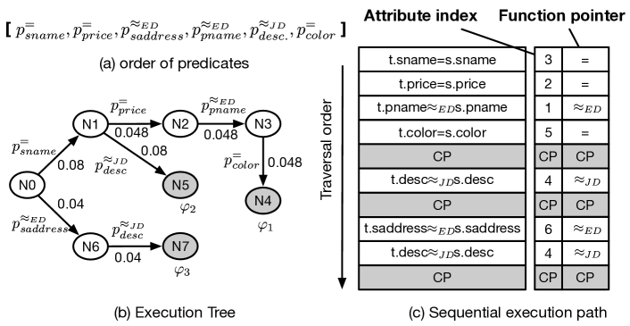
Figure 4. Execution tree

Intuitively, given $(t_{1},t_{2})$ and $\varphi\in\Delta$, if $\varphi$ is more likely to be a witness at $(t_{1},t_{2})$, it should be evaluated earlier. Motivated by this, we compute the probability for $\varphi:X\rightarrow l$ to be a witness on $D$ as:

$${\mathsf{wp}}(\varphi,D)=\prod_{p\in X}{\mathsf{sp}}(p,D),\vspace{-0.7ex}$$

if we assume the satisfaction of predicates as independent events; intuitively, if all predicates in $X$ are satisfied, $\varphi$ is a witness. If this does not hold, we can reuse historical logs and estimate ${\mathsf{wp}}(\varphi,D)$, to be the proportion of historical pairs such that $\varphi$ is a witness. Since the evaluation of $\mathsf{MDs}$ in $\Delta$ is guided by edge scores during DFS on ${\mathcal{T}}$, below we define the score of a given edge $e$ based on ${\mathsf{wp}}(\varphi,D)$.

Edge score. For each $\mathsf{MD}$ $\varphi$, we denote by $\rho_{\varphi}$ the path of ${\mathcal{T}}$ from root to the leaf whose associated $\mathsf{MD}$ is $\varphi$. We compute the set of $\mathsf{MDs}$ $\varphi$ in $\Delta$ such that the given edge $e$ is part of $\rho_{\varphi}$ and denote it by $\Psi_{e}$, i.e., $\Psi_{e}=\{\varphi\in\Delta\mid e$ is part of $\rho_{\varphi}\}$. The score of edge $e$ is ${\mathsf{score}}(e)=\max_{\rho_{\varphi}\in\Psi_{e}}{\mathsf{wp}}(\varphi,D)$. This said, edges leading to promising $\mathsf{MDs}$ will have high scores and thus, will be explored early via DFS on ${\mathcal{T}}$.

Example 5.

Let ${\mathsf{sp}}(p_{\mathsf{sname}}^{=},D)=0.4$ and ${\mathsf{sp}}(p_{\mathsf{description}}^{\approx_{\mathsf{JD}}},D)=0.2$. Then ${\mathsf{wp}}(\varphi_{2},D)=0.4\times 0.2=0.08$. Assume that we also compute ${\mathsf{wp}}(\varphi_{1},D)=0.048$. Then the score of edge $e=(N_{0},N_{1})$ is $\max\{\allowbreak{\mathsf{wp}}(\varphi_{1},D),\allowbreak{\mathsf{wp}}(\varphi_{2},D)\}$ = 0.08, since $e$ is part of both $\rho_{\varphi_{1}}$ and $\rho_{\varphi_{2}}$.

Complexity. It takes EPG $O(c_{\mathsf{unit}}|{\mathcal{P}}|+|{\mathcal{P}}|\log(|{\mathcal{P}}|)+|\varphi||\Delta|)$ time to generate the execution plan, where $c_{\mathsf{unit}}$ is the unit time for computing the cost-effectiveness of a predicate. This is because the predicate ordering can be obtained in $O(c_{\mathsf{unit}}|{\mathcal{P}}|+|{\mathcal{P}}|\log(|{\mathcal{P}}|))$ time and the tree can be constructed in $(|\varphi||\Delta|)$ time, by scanning $\Delta$ once.

Remark. As a by-product of ensuring the predicate ordering and DFS tree traversal, we can reuse the evaluation results of common “prefix” predicates (i.e., common predecessors in ${\mathcal{T}}$). Moreover, if a tuple pair fails to satisfy the predicate associated with edge $(N,N_{c})$ in ${\mathcal{T}}$, the evaluation of all descendants of $N_{c}$ is bypassed directly.

Example 6.

We evaluate ${\mathcal{T}}$ in Figure 4(b) for $(t_{1},t_{5})$ in $D$. After evaluating $p_{\mathsf{sname}}^{=}$, we find that $h(t_{1},t_{5})\allowbreak\not\models p_{\mathsf{description}}^{\approx_{\mathsf{JD}}}$ and thus we cannot move to $N_{5}$. Then DFS will return back to $N_{1}$ and continue to check unexplored children of $N_{1}$ (i.e., $N_{2}$). In this way, the common “prefix” predicate $p_{\mathsf{sname}}^{=}$ of $\varphi_{1}$ and $\varphi_{2}$ is only evaluated once.

5. Optimizations and Scheduling

As remarked earlier, GPUs adopt SIMT execution, where a thread is idle if other threads take longer (i.e., thread divergence). Below are sources of divergence (some are specific to rule-based blocking).

• Conditional statements. GPUs may execute different paths in conditional statements (Section 2), e.g., one pair may be quickly identified as a potential match if the first $\mathsf{MD}$ checked is its witness, while another is found as a mismatch until all $\mathsf{MDs}$ are iterated.

• Data-dependent execution. The execution depends on the data being processed, e.g., even for the same predicate, the evaluation time on different tuples is different (e.g., long vs. short text).

• Imbalanced workloads. If the workload assigned to each thread is not evenly distributed, some may complete faster than others.

While thread divergence is a general issue in GPU-programming, rule-based blocking offers some unique opportunities to mitigate it, e.g., the evaluations of distinct pairs are often independent tasks, making it possible to (a) assign approximately equal tasks to threads, to enable workload balancing, and (b) “steal” tasks from other threads, to cope with different execution paths and data-dependent execution. Below we present the hardware-aware optimization and scheduling techniques that exploit GPU characteristics for massive parallelism, including: (a) efficient device execution of an execution plan (Section 5.1), (b) strategies to mitigate divergence (Section 5.2), (c) collaboration of multiple GPUs (Section 5.3) and more in (ful, 2024).

5.1. Execution plan on GPUs

The execution plan ${\mathcal{T}}$, initially generated on CPUs, will undergo the evaluation on GPUs in a DFS manner. However, DFS tree traversal is typically recursively implemented, which is not efficient on GPUs. It may exacerbate divergence since each call adds a recursive function to the stack and incurs message payloads (see Section 6). Moreover, although we can reuse “prefix” predicates via DFS, some predicates may still be evaluated repeatedly, e.g., $p_{\mathsf{description}}^{\approx_{\mathsf{JD}}}$ in $\varphi_{2}$ and $\varphi_{3}$. Optimized structures are required to harness the power of GPUs.

Tree traversal on GPUs. Note that upon completion of the tree construction, the evaluation order is fixed. Thus the DFS traversal of the tree on CPUs can be translated to a sequential execution path, which is an ordered list of predicates, on GPUs (see Figure 4(c) for the sequential execution path of the tree in Example 2).

We maintain two structures for each predicate $p$ in the execution path: an index buffer and a function pointer buffer, which store the indices of attributes compared in $p$, and the function pointer of the comparison operator in $p$, respectively, e.g., for predicate $p_{\mathsf{sname}}^{=}:t.{\mathsf{sname}}=s.{\mathsf{sname}}$, its comparison operator is “=” and its attribute index is 3 since $\mathsf{sname}$ is the 3rd attribute in schema $\mathsf{Products}$. In addition, at the end of each rule, we set a checkpoint ($\mathsf{CP}$). When a GPU thread encounters a $\mathsf{CP}$, it knows that the undergoing tuple pair satisfies a rule and it can skip the subsequent computation.

Reusing computation. To avoid repeated evaluation, we additionally maintain a bitmap for all predicates on GPUs. The bit of a predicate $p$ is set to true if $p$ has been evaluated. If this is the case, we can directly reuse previous results. This bitmap can also be used for symmetric predicates (i.e., $h(t_{1},t_{2})\models p$ iff $h(t_{2},t_{1})\models p$).

Note that to be general, we do not make the assumption that a witness $\varphi$ at $(t_{1},t_{2})$ is also a witness at $(t_{2},t_{1})$, due to, e.g., asymmetric similarity comparison (Section 2). However, we can extend $\mathsf{HyperBlocker}$ if such assumption holds, by maintaining a bitmap to avoid repeated evaluation for $(t_{2},t_{1})$ if $(t_{1},t_{2})$ is already evaluated.

5.2. Divergence mitigation strategies

To further mitigate divergence, we propose two GPU-oriented strategies, namely parallel sliding windows (PSW) and task-stealing.

Parallel sliding windows (PSW). Given a partition $P$, PSW processes it with only a few index jumps; it also helps GPUs evenly distribute workloads across SMs. Specifically, PSW works in 3 steps:

(1) We divide $P$ into $\frac{|P|}{n_{t}}$ intervals, where each interval consists of $n_{t}$ tuples. These intervals are processed with a fixed-size window, which slides the intervals from left to right. Within each window, we assign an interval to a Thread Block (TB) with warps of 32 threads; each thread in the TB is responsible for a tuple $t_{i}$ in the interval.

(2) Assume that a thread is responsible for tuple $t_{i}$. Then this thread compares $t_{i}$ with all the other tuples, say $t_{j}$, in $P$ according to the execution plan ${\mathcal{T}}$ and decides whether $(t_{i},t_{j})$ is a potential match.

(3) When all threads of a TB finish, this TB writes the results back to the host memory and it will move on to process the next interval in the next sliding window until the window reaches the end.

Note that in total, it requires $\frac{|P|}{n_{t}n_{w}}$ sequential index jumps for each TB, where $n_{w}$ is the size of the sliding window.

Example 1.

As shown in Figure 5, a data partition $P$ is divided 9 intervals and the size of the sliding window is 3 (i.e., $n_{w}=3$). Interval 1 is assigned to TB1, where each thread in TB1 will compare a tuple in Interval 1 with all other tuples in $P$. When all threads of TB1 finish evaluation, TB1 moves on to process Interval 4.

Remark. Note that PSW achieves tuple-level parallelism (i.e., tuples are evaluated in parallel; each thread is responsible for a tuple). There are other design choices for parallelism, e.g., rule-level, predicate-level and token-level parallelisms, so that the entire warp is assigned to a tuple pair and rules, predicates and tokens in text are evaluated in parallel, respectively (one thread per rule/predicate/token, see (ful, 2024) for more). However, these designs may exacerbate divergence, due to, e.g., synchronization cost (e.g., one thread has to wait for results from other threads to make a final decision), or incur unnecessary computation, e.g., when a thread finds a witness $\varphi$ at $(t_{1},t_{2})$ (resp. a predicate $p$ in $\varphi$ such that $h(t_{1},t_{2})\not\models p$), other threads may still check other rules in $\Delta$ (resp. other predicates in $\varphi$).

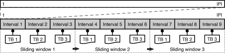
Figure 5. Parallel sliding windows

Task-stealing. Although each TB will process roughly equal intervals, the execution time of different intervals is not the same, due to conditional statements and data-dependent execution remarked earlier. This said, the workloads of all TBs can still be imbalanced.

Example 2.

Continuing Example 1, three TBs process 9 intervals in Figure 6(a). Even though each TB is assigned 3 intervals, the execution times can still skew, e.g., the total time units required by TB1 and TB3 are 10 and 3, respectively, i.e., TB3 is idle for 7 time units.

Below we introduce both the inter-interval and intra-interval task-stealing strategies to further balance the workloads.

Inter-interval task-stealing. It is commonly observed that the execution times of some TBs are longer than the others. In this case, a large number of TBs are idle, waiting for the slowest TB.

In light of this, we employ an inter-interval task-stealing strategy. Specifically, we maintain a bitmap in global memory, where each bit indicates the status of an interval, so that TBs can steal not-yet-processed intervals from each other. Each TB processes intervals in two stages: (a) It first processes its assigned intervals one by one. Whenever a TB starts to process an interval, the bitmap is checked. If the bit of the interval is false (i.e., not yet processed), it processes this interval and sets the bit true. (b) If this TB is idle after finishing all assigned intervals, it traverses the bitmap to steal a not-yet-processed interval, by setting the corresponding bit true and processing that interval. Other TBs will skip an interval if it has been stolen.

Example 3.

In Example 2, TB3 finishes its assigned intervals after 3 time units. Then it checks the bitmap and steals Interval 4; similarly for TB2. Compared with the time in Figure 6(a), the total time units are reduced from 10 to 7 after stealing in Figure 6(b).

Intra-interval task-stealing. Recall that a thread for $t_{i}$ will compare $t_{i}$ with other tuples in $P$. Since the evaluation of distinct pairs is independent, we can even steal tasks from executing intervals. To facilitate this, we maintain two integers $\mathsf{start}$ and $\mathsf{end}$, initialized to 1 and $|P|$, respectively, indicating the remaining range of tuples to be compared with $t_{i}$. Then this thread starts to evaluate $(t_{i},t_{{\mathsf{start}}})$. Upon completion, it sets ${\mathsf{start}}={\mathsf{start}}+1$ and moves on to the next pair $(t_{i},\allowbreak t_{{\mathsf{start}}})$. When ${\mathsf{start}}={\mathsf{end}}$, this thread finishes all evaluation for $t_{i}$.

Based on this, the intra-interval task-stealing works as follows. If TB_a finishes all assigned intervals and there are no not-yet-processed intervals, it finds an executing TB_b and iterates all threads in TB_b, so that the $i$-th thread in TB_a steals half workload (i.e., half pairs to be compared) from the $i$-th thread in TB_b. Assume the integers maintained for the $i$-th thread in TB_b (resp. TB_a) are ${\mathsf{start}}_{b}$ and ${\mathsf{end}}_{b}$ (resp. ${\mathsf{start}}_{a}$ and ${\mathsf{end}}_{a}$). We set ${\mathsf{start}}_{a}={\mathsf{start}}_{b}+\frac{{\mathsf{start}}_{b}+{\mathsf{end}}_{b}}{2}$, ${\mathsf{end}}_{a}={\mathsf{end}}_{b}$, and ${\mathsf{end}}_{b}=\allowbreak{\mathsf{start}}_{b}+\frac{{\mathsf{start}}_{b}+{\mathsf{end}}_{b}}{2}-1$, i.e., the latter half of tuples remained to be compared is stolen from each thread in TB_b.

Example 4.

Continuing Example 3, when TB3 finishes Interval 4 stolen from TB1 in Figure 6(b), it finds no not-yet-processed intervals. However, since TB2 is still evaluating Interval 7, TB3 steals half remaining workload from it, saving 1 more time unit (Figure 6(c)).

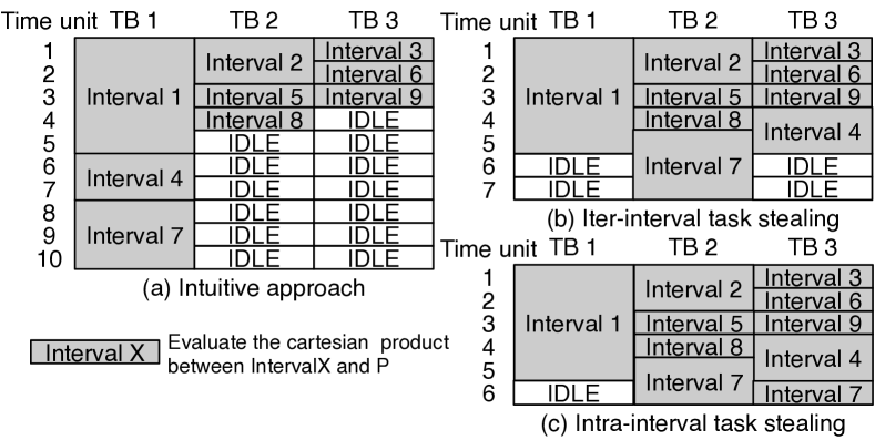
Figure 6. Task-stealing

5.3. GPU collaboration

A GPU server nowadays usually has multiple GPUs connected via NVLink (Li et al., 2019) or PCIe. Scaling blocking to multiple GPUs is beneficial for jointly utilizing the computation and storage powers of GPUs.

In pursuit of this, one can split data evenly so that each GPU handles exactly one (Pandey et al., 2019), or assign multiple partitions to each GPU in a round-robin manner (Rossi and Zhou, 2016). These, however, do not work well since (a) workload can be imbalanced due to skewed execution times of partitions (see statistic in (ful, 2024)), (b) pending partitions may wait when multiple partitions compete for limited PCIe bandwidth or CUDA cores (see Section 2) and (c) they independently conduct blocking on partitions and do not effectively handle scenarios where $t_{i}$ and $t_{j}$ reside on different partitions, resulting in elevated false-negative rates. To address this issue, one can duplicate tuples in multiple partitions (Deng et al., 2022; Chu et al., 2016), but it incurs both memory and data transfer costs.

In light of these, we present a collaborative approach integrating partitioning and scheduling strategies, where the former aims at minimizing data redundancy while reducing false negatives and the latter prioritizes load balancing and minimizes resource contention.

Data partitioning. A typical method for data partitioning computes a hash key for each tuple based on some attributes and tuples with same hash key are grouped together. Instead of sacrificing the accuracy (e.g., using only one hash function) or unnecessarily duplicating tuples, $\mathsf{HyperBlocker}$ applies $s$ hash functions to obtain $s$ partition-keys, where $s$ is the number of children $N_{c}$ of the root node $N_{0}$ in the execution tree ${\mathcal{T}}$; each hash function is constructed from the predicate $p$ associated with an edge $(N_{0},N_{c})$. In this way, the predicates that we adopt for data partitioning are those prioritized by ${\mathcal{T}}$, e.g., given $p_{\mathsf{sname}}^{=}$ associated with ($N_{0},N_{1}$) in Figure 4(b), we hash tuples in $D$ based on their values in $\mathsf{sname}$. The benefits are two-fold: (1) According to the construction of ${\mathcal{T}}$, these hash functions are selective and might be shared by rules, i.e., we can achieve good hashing with a few hashing functions. (2) We can assign each tuple a branch ID, indicating the hash function used. Only tuples that share the same hash function are compared, thereby reducing redundant computations incurred by multiple hash functions.

Scheduling. $\mathsf{HyperBlocker}$ adopts a two-step scheduling strategy. Initially, data partitions and GPUs are hashed to random locations on a unit circle (Mirrokni et al., 2018). If a partition $P_{i}$ is assigned to an ineligible GPU (where there is no idle core or available PCIe bandwidth), it is rerouted to the nearest available GPU in a clockwise direction.

Remark. If data partitioning is done by a hashing function from a similarity predicate $p$, it is possible that $h(t_{1},t_{2})\models p$ but $t_{1}$ and $t_{2}$ reside on different partitions, leading to potential false negatives in blocking. In this case, a CUDA kernel (CUD, 2024) with local data $P_{i}$ can optionally “pull” partition $P_{j}$ from another kernel and evaluate ${\mathcal{T}}$ across $P_{i}$ and $P_{j}$. The pull operation retrieves data from locations outside $P_{i}$, depending on whether $P_{i}$ and $P_{j}$ reside on the same GPU. If $P_{i}$ and $P_{j}$ reside on the same GPU, the pull operation is executed directly without any data transfer. Otherwise, the pull operation for $P_{j}$ can be carried out using cudaMemcpyPeer() to take the advantages of high bandwidth and low latency provided by NVLink.

6. Experimental Study

We evaluated $\mathsf{HyperBlocker}$ for its accuracy-efficiency and scalability. We also conducted sensitivity tests and ablation studies.

Experimental setup. We start with the experimental setting.

Table 2. Datasets

Dataset	Domain	#Tuples	Max #Pairs	#GT Pairs	#Attrs	#Rules	#Partitions
$\mathsf{Fodors}$-$\mathsf{Zagat}$	restaurant	866	$1.8\times 10^{4}$	112	6	1	1
$\mathsf{DBLP}$-$\mathsf{ACM}$	citation	4591	$6.0\times 10^{6}$	2294	4	10	8
$\mathsf{DBLP}$-$\mathsf{Scholar}$	citation	66881	$1.7\times 10^{8}$	5348	4	10	8
$\mathsf{IMDB}$	movie	1.5M	$8.1\times 10^{10}$	0.2M+	6	10	128
$\mathsf{Songs}$	music	0.5M	$2.7\times 10^{11}$	1.2M	8	10	128
$\mathsf{NCV}$	vote	2M	$1.0\times 10^{12}$	0.5M+	5	10	512
$\mathsf{TFACC}$	traffic	10M	$1.0\times 10^{14}$	#	16	50	1024
$\mathsf{TFACC_{large}}$	traffic	36M	$1.3\times 10^{15}$	#	16	50	1024

Datasets. We used eight real-world public datasets in Table 2, which are widely adopted ER benchmarks and real-life datasets (mag, 2021; MOT, 2024; Ded, 2021). Most datasets (except $\mathsf{TFACC}$ and ${\mathsf{TFACC}}_{\mathsf{large}}$) have labeled matches or mismatches as the ground truths (GT). For datasets without ground truths, we assume the original datasets were correct, and randomly duplicated tuples as noises (Fan et al., 2021). The training data consists of 50% of ground truths and 50% of randomly selected noise.

Baselines. As remarked in Section 2, although $\mathsf{HyperBlocker}$ is designed as a blocker, it can be used with or without a matcher. Thus, below we not only compared $\mathsf{HyperBlocker}$ against widely used blockers but also integrated ER solutions (i.e., blocker + matcher).

We compared three distributed ER systems: (1) $\mathsf{Dedoop}$ (Kolb et al., 2012a; cod, 2021a), (2) $\mathsf{SparkER}$ (Gagliardelli et al., 2019; cod, 2024b), (3) $\mathsf{DisDedup}$ (Chu et al., 2016; cod, 2024a), where $\mathsf{DisDedup}$ is the SOTA CPU-based parallel ER system, designed to minimize communication and computation costs; $\mathsf{Dedoop}$ focuses on optimizing computation cost; $\mathsf{SparkER}$ integrates Blast blocking (Simonini et al., 2016) on Spark (spa, 2024).

We also compared four GPU-based baselines: (4) $\mathsf{DeepBlocker}$ (Thirumuruganathan et al., 2021), (5) $\mathsf{GPUDet}$ (Forchhammer et al., 2013), (6) $\mathsf{Ditto}$ (Li et al., 2020a; cod, 2021b), (7) ${\mathsf{DeepBlocker}}_{\mathsf{Ditto}}$, where $\mathsf{DeepBlocker}$ is the SOTA DL-based blocker, $\mathsf{GPUDet}$ implements well-known similarity algorithms for tuple pair comparison, $\mathsf{Ditto}$ is the SOTA matcher, and ${\mathsf{DeepBlocker}}_{\mathsf{Ditto}}$ uses $\mathsf{DeepBlocker}$ as the blocker and $\mathsf{Ditto}$ as the matcher, respectively. Note that $\mathsf{Ditto}$ takes tuple pairs as input, instead of relations/partitions as other methods. Due to the high cost of $\mathsf{Ditto}$, it is infeasible to feed the Cartesian product of data to $\mathsf{Ditto}$. Thus, for each tuple in ground truths, we adopted a similarity-join method $\mathsf{Faiss}$ (Johnson et al., 2021) to get the top-2 nearest neighbors, as a preprocessing step of $\mathsf{Ditto}$. Denote the resulting baseline by ${\mathsf{Ditto}}_{\mathsf{top2}}$. Since $\mathsf{Faiss}$ often serves as a key component of many ER solutions (Ebraheem et al., 2018; Thirumuruganathan et al., 2021), we also compared $\mathsf{Faiss}$ in (ful, 2024).

Besides, we also implemented several variants: (1) $\mathsf{HyperBlocker}$, the basic blocker with all optimizations. (2) ${\mathsf{HyperBlocker}}_{\mathsf{Ditto}}$, an improved version that uses $\mathsf{HyperBlocker}$ as the blocker and $\mathsf{Ditto}$ as the matcher, respectively. Note that ${\mathsf{HyperBlocker}}_{\mathsf{Ditto}}$ is particularly compared against ${\mathsf{Ditto}}_{\mathsf{top2}}$ to show how we speed up the overall ER. (3) ${\mathsf{HyperBlocker}}_{\mathsf{noEPG}}$, a variant without EPG (Section 4). (4) ${\mathsf{HyperBlocker}}_{\mathsf{noHO}}$ that disables all hardware optimizations (Section 5). We also compared more designated variants in Exp 3-5.

Table 3. Comparison with the SOTA DL-based blocker

Method	Metric	Dataset
		Fodors-Zagat	DBLP-Scholar	DBLP-ACM
$\mathsf{DeepBlocker}$	$\mathsf{Rec}$ ($\%$)	100 (+0)	98 (+5)	98 (+4)
	$\mathsf{CSSR}$ (‱)	15.1 (+14.5)	2.3 (+1.1)	2.2 (+1.8)
	Time (s)	6.1 (122$\times$)	72.8 (11.0$\times$)	8.0 (10.0$\times$)
	Host Mem. cost (GB)	9.9 (49.5$\times$)	14.0 (23.3$\times$)	10.3 (34.3$\times$)
	Device Mem. cost (GB)	0.9 (1.8$\times$)	1.1 (1.6$\times$)	0.9 (1.5$\times$)
$\mathsf{HyperBlocker}$	$\mathsf{Rec}$ ($\%$)	100	93	94
	$\mathsf{CSSR}$ (‱)	0.6	1.2	0.4
	Time (s)	0.05	6.6	0.8
	Host Mem. cost (GB)	0.2	0.6	0.3
	Device Mem. cost (GB)	0.5	0.7	0.6

Rules. We mined $\mathsf{MDs}$  using (Song and Chen, 2013) and the number of $\mathsf{MDs}$ is shown in Table 2. We checked the $\mathsf{MDs}$ manually to ensure correctness.

Table 4. Accuracy & runtime on benchmarks where “*” denotes that integrating $\mathsf{HyperBlocker}$ with $\mathsf{Ditto}$ does not improve the F1-score and thus we report the result of $\mathsf{HyperBlocker}$, and “/” denotes that the F1-score cannot be computed within 3 hours.

Method	Backend	Category	DBLP-ACM		IMDB		Songs		NCV
			F1-score	Time (s)	F1-score	Time (s)	F1-score	Time (s)	F1-score	Time (s)
$\mathsf{SparkER}$	CPU	Blocker	0.77 (-0.17)	11.0 (13.8$\times$)	0.31 (-0.65)	242.9 (6.8$\times$)	0.08 (-0.72)	203.4 (15.2$\times$)	0.26 (-0.66)	229.3 (49.8$\times$)
$\mathsf{GPUDet}$	GPU	Blocker	0.92 (-0.02)	20.1 (25.1$\times$)	0.94 (-0.02)	323.8 (9.1$\times$)	0.80 (+0)	404.8 (30.2$\times$)	0.90 (-0.02)	1252.6 (272.3$\times$)
$\mathsf{DeepBlocker}$	GPU	Blocker	0.98 (+0.04)	8.3 (10.4$\times$)	/	¿3h	/	¿3h	/	¿3h
${\mathsf{HyperBlocker}}_{\mathsf{noEPG}}$	GPU	Blocker	0.94 (+0)	9.9 (12.4$\times$)	/	$>$3h	0.80 (+0)	1904.1 (142$\times$)	0.92 (+0)	2408.6 (523.6$\times$)
${\mathsf{HyperBlocker}}_{\mathsf{noHO}}$	GPU	Blocker	0.94 (+0)	9.5 (11.9$\times$)	0.96 (+0)	472.6 (13.2$\times$)	0.80 (+0)	45.0 (3.4$\times$)	0.92 (+0)	35.9 (7.8$\times$)
$\mathsf{HyperBlocker}$	GPU	Blocker	0.94	0.8	0.96	35.7	0.80	13.4	0.92	4.6
$\mathsf{Dedoop}$	CPU	Blocker+Matcher	0.90 (-0.08)	59.4 (9.4$\times$)	0.67 (-0.29)	534.0 (15.0$\times$)	0.80 (-0.08)	7643.4 (6.5$\times$)	/	$>$3h
$\mathsf{DisDedup}$	CPU	Blocker+Matcher	0.45 (-0.53)	94.0 (14.9$\times$)	0.67 (-0.29)	644.0 (18.0$\times$)	0.06 (-0.82)	917.0 (0.8$\times$)	/	$>$3h
${\mathsf{Ditto}}_{\mathsf{top2}}$	GPU	Blocker+Matcher	0.98 (+0)	9.0 (1.4$\times$)	0.79 (-0.17)	6741.2 (188.8$\times$)	0.88 (+0)	2308.6 (2.0$\times$)	0.97 (+0.03)	381.8 (2.1$\times$)
${\mathsf{DeepBlocker}}_{\mathsf{Ditto}}$	GPU	Blocker+Matcher	0.99 (+0.01)	12.4 (2.0$\times$)	/	¿3h	/	¿3h	/	¿3h
${\mathsf{HyperBlocker}}_{\mathsf{Ditto}}$	GPU	Blocker+Matcher	0.98	6.3	*0.96	*35.7	0.88	1179.0	0.94	180.6

Measurements. Following typical ER settings, we measured the performance of each method (blocker, matcher, or the combination of the two) in terms of the runtime and the F1-score, defined as F1-score = $\frac{2\times{\mathsf{Prec}}\times{\mathsf{Rec}}}{{\mathsf{Prec}}+{\mathsf{Rec}}}$. Here ${\mathsf{Prec}}$ is the ratio of correctly identified tuple pairs to all identified pairs and ${\mathsf{Rec}}$ is the ratio of correctly identified tuple pairs to all pairs that refer to the same real-world entity. All methods aim to achieve high ${\mathsf{Rec}}$, ${\mathsf{Prec}}$ and F1-scores. Following (Thirumuruganathan et al., 2021), we also report the candidate set size ratio (CSSR), defined as $\frac{|{\mathsf{Ca}}(P)|}{|P|\times|P|}$, when comparing $\mathsf{HyperBlocker}$ with $\mathsf{DeepBlocker}$, to show the portion of tuple pairs that require further comparison by the matcher, i.e., the smaller the CSSR, the better the blocker.

Environment. We run experiments on a Ubuntu 20.04.1 LTS machine powered with 2 Intel Xeon Gold 6148 CPU @ 2.40GHz, 4TB Intel P4600 PCIe NVMe SSD, 128GB memory, and 8 Nvidia Tesla V100 GPUs with the widely adopted hybrid cube-mesh topology (see more in (NVIDIA, 2024)). The programs were compiled with CUDA-11.0 and GCC 7.3.0 with -O3 compiler. $\mathsf{DisDedup}$, $\mathsf{SparkER}$, and $\mathsf{Dedoop}$ were run on a cluster of 30 HPC servers, powered with 2.40GHz Intel Xeon Gold CPU, 4TB Intel P4600 SSD, 128GB memory.

Default parameters. Unless stated explicitly, we used the following default parameters, which are best-tuned on each dataset via gird search (Jiménez et al., 2008). Intuitively, gird search is a practical method for systematically exploring the parameter space to get the set of parameters that results in the best performance. The maximum number of predicates in an $\mathsf{MD}$ is 10. The number $m$ of data partitions is given in Table 2. The sizes of intervals and sliding windows, namely $n_{t}$ and $n_{w}$, are 256 and 1024, respectively. For the offline model ${\mathcal{N}}$, we adopted a regression model with 3 hidden layers, with 2, 6, and 1 neurons, respectively. We used ReLU (Nair and Hinton, 2010) as the activation function and Adam (Kingma and Ba, 2015) as the optimizer. We used one GPU by default.

Experimental results. For lack of space, we report our findings on some datasets as follows; consistent on others datasets (more in (ful, 2024)).

Exp-1: Motivation study. We motivate our study by comparing $\mathsf{HyperBlocker}$, our rule-based blocker, with the SOTA DL-based blocker $\mathsf{DeepBlocker}$ (Table 3), where the bracket next to a metric of $\mathsf{DeepBlocker}$ gives its difference or deterioration factor to ours.

DL-based blocking vs. rule-based blocking. We report recall, CSSR, runtime, and (host and device) memory for both methods. Consistent with (Thirumuruganathan et al., 2021), for $\mathsf{DeepBlocker}$, each tuple was paired with top-$K$ similar tuples as initial candidate pairs, where $K=5$ on all datasets (except $\mathsf{DBLP}$-$\mathsf{Scholar}$ where $K=150$). As remarked in Section 1, both methods have strengths. (1) $\mathsf{HyperBlocker}$ effectively reduces the number of pairs to further compare while maintaining high $\mathsf{Rec}$ (¿93%), e.g., its average $\mathsf{CSSR}$ is 5.8‱ less than $\mathsf{DeepBlocker}$. (2) $\mathsf{HyperBlocker}$ is at least 10$\times$ faster. (3) $\mathsf{HyperBlocker}$ consumes less memory than $\mathsf{DeepBlocker}$, e.g., the host memory it consumes is at least 23.3$\times$ less than $\mathsf{DeepBlocker}$. (4) Note that the $\mathsf{Rec}$ of $\mathsf{HyperBlocker}$ is slightly lower than $\mathsf{DeepBlocker}$, which is acceptable given its convincing speedup and memory saving, since the primary goal of a blocker is to improve the efficiency and scalability of ER, not to improve the accuracy of ER (the goal of a matcher).

Exp-2: Accuracy-efficiency. We report the F1-scores and runtime of all blockers and integrated ER solutions (i.e., blocker + matcher) in Table 4. Here $\mathsf{DeepBlocker}$ pairs each tuple with its top-2 tuples as initial candidate pairs. For all blockers, the bracket next to each F1-score (resp. time) gives the difference (resp. slowdown) in F1-score (resp. time) to $\mathsf{HyperBlocker}$ (marked yellow). For a fair comparison, the brackets of each integrated ER solution give the difference compared with ${\mathsf{HyperBlocker}}_{\mathsf{Ditto}}$ (marked yellow).

Accuracy. We mainly analyze the F1-scores of $\mathsf{HyperBlocker}$, which are consistently above 0.8 over all datasets. Besides, we find:

(1) $\mathsf{HyperBlocker}$ outperforms CPU-based distributed solutions, e.g., it achieves up to 0.29, 0.74, and 0.72 improvement in F1-score against $\mathsf{Dedoop}$, $\mathsf{DisDedup}$, and $\mathsf{SparkER}$, respectively, even though the former two are integrated with matchers. This is because these solutions exploit data partition-based parallelism only, which may lead to false negatives if matched tuples are put into different partitions.

(2) Compared with the four GPU-based baselines, $\mathsf{HyperBlocker}$ has comparable accuracy. In particular, it even beats ${\mathsf{Ditto}}_{\mathsf{top2}}$, the SOTA matcher, by 0.17 F1-score in $\mathsf{IMDB}$. This shows that even without a matcher, $\mathsf{HyperBlocker}$ alone is already accurate in certain cases. Moreover, $\mathsf{DeepBlocker}$ and ${\mathsf{DeepBlocker}}_{\mathsf{Ditto}}$ struggle to handle large datasets. When facing million-scale data, they cannot finish in 3 hours. This again motivates the need for rule-based alternatives.

(3) Combing $\mathsf{HyperBlocker}$ with ${\mathsf{Ditto}}$, ${\mathsf{HyperBlocker}}_{\mathsf{Ditto}}$ further boosts the accuracy, achieving the best F1-score in $\mathsf{Songs}$. Nevertheless, DL-based solutions still have the best F1-scores in other cases, justifying that none of them can dominate the other in all cases.

(4) ${\mathsf{HyperBlocker}}_{\mathsf{noEPG}}$ and ${\mathsf{HyperBlocker}}_{\mathsf{noHO}}$ are as accurate as $\mathsf{HyperBlocker}$, since they only differ in the optimizations.

Runtime. We next report the runtime. (1) $\mathsf{HyperBlocker}$ runs substantially faster than all baselines, e.g., it is at least 6.8$\times$, 9.1$\times$, 10.4$\times$, 15.0$\times$, 18.0$\times$, 11.3$\times$ and 15.5$\times$ faster than $\mathsf{SparkER}$, $\mathsf{GPUDet}$, $\mathsf{DeepBlocker}$, $\mathsf{Dedoop}$, $\mathsf{DisDedup}$, $\mathsf{Ditto}$, and ${\mathsf{DeepBlocker}}_{\mathsf{Ditto}}$ respectively. (2) ${\mathsf{HyperBlocker}}_{\mathsf{Ditto}}$ is slower than $\mathsf{HyperBlocker}$ as expected since it performs additional matching. Nonetheless, ${\mathsf{HyperBlocker}}_{\mathsf{Ditto}}$ is at least 1.4$\times$ (resp. 2.0$\times$) faster than ${\mathsf{Ditto}}_{\mathsf{top2}}$ (resp. ${\mathsf{DeepBlocker}}_{\mathsf{Ditto}}$). Given its comparable F1-score, we substantiate our claim (Section 1) that blocking is a crucial part of the overall ER process. (3) $\mathsf{HyperBlocker}$ is at least 12.4$\times$ and 3.4$\times$ faster than ${\mathsf{HyperBlocker}}_{\mathsf{noEPG}}$ and ${\mathsf{HyperBlocker}}_{\mathsf{noHO}}$, respectively, verifying the usefulness of execution plans and hardware optimizations.

Impact of $m$. Figure 7 (a) reports how the number $m$ of data partitions affects the recall (the right y-axis) and the runtime (the left y-axis) on $\mathsf{NVC}$. As shown there, both metrics of $\mathsf{HyperBlocker}$ decreases with increasing $m$. This is because when there are more partitions, both the number of pairwise comparisons and the candidate matches that can be identified in each partition are reduced.

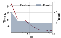
(a) $\mathsf{NVC}$: Impact of $m$

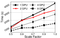
(b) $\mathsf{TFACC}$-$\mathsf{Large}$: Varying #GPUs

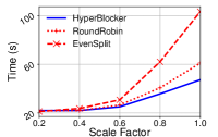
(c) $\mathsf{IMDB}$: Impact of schedulers

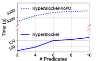
(d) $\mathsf{TFACC}$: Varying $|\varphi|$

(e) $\mathsf{TFACC}$: Varying $|\Delta|$

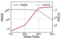
(f) $\mathsf{DBLP}$-$\mathsf{ACM}$: Varying noise%

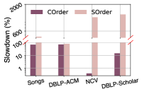
(g) More ordering strategies

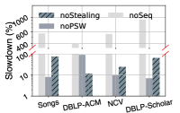
(h) Ablation study

Figure 7. Efficiency, scalability, and effectiveness of $\mathsf{HyperBlocker}$

Exp-3: Scalability. We tested our scalability under multi-GPUs scenarios. The default number of GPUs is 4 in this set of experiments.

Varying $|D|$/#GPUs. We varied the scale factor of $D$ in $\mathsf{TFACC_{large}}$ and tested $\mathsf{HyperBlocker}$ with different numbers of GPUs in Figure 7(b). $\mathsf{HyperBlocker}$ scales well with data sizes, e.g., with 8 GPUs, it takes 1604s to process 36M tuples; this is not feasible for both CPU- and GPU-based baselines. When the number of GPUs changes from 1 to 8, $\mathsf{HyperBlocker}$ is 2.6$\times$ faster, since $\mathsf{HyperBlocker}$ mainly accelerates the operations on GPUs, while other parts of the system (e.g., I/O and data partitioning) may also limit the overall performance.

Impact of task schedulers. We tested the impact of task schedulers, by comparing $\mathsf{HyperBlocker}$ with two variants, that uses $\mathsf{EvenSplit}$ and $\mathsf{RoundRobin}$ for scheduling (Section 5.3), respectively, by varying $|D|$ in Figure 7(c). $\mathsf{HyperBlocker}$ works better than the two, e.g., when the scale factor is 100%, $\mathsf{HyperBlocker}$ is 1.3$\times$ and 2.2$\times$ faster than $\mathsf{RoundRobin}$ and $\mathsf{EvenSplit}$, respectively, since both variants may limit CUDA’s ability of dynamically scheduling tasks.

Exp-4: Tests on EPG (Section 4). We evaluated EPG (and its offline model ${\mathcal{N}}$) and justified the need of effective evaluation orders.

Varying $|\varphi|$. We tested the number $|\varphi|$ of predicates in each $\mathsf{MD}$ $\varphi$ against ${\mathsf{HyperBlocker}}_{\mathsf{noPO}}$ that evaluates predicates in a random order in $\mathsf{TFACC}$ (Figure 7(d)). (1) $\mathsf{HyperBlocker}$ takes longer with larger $|\varphi|$, as expected. (2) $\mathsf{HyperBlocker}$ is feasible in practice, e.g., when $|\varphi|=10$, it only takes 135.2s. (3) On average, $\mathsf{HyperBlocker}$ shows 32.5$\times$ speedup to ${\mathsf{HyperBlocker}}_{\mathsf{noPO}}$. This justifies the importance of predicate ordering in efficient rule-based blocking.

Varying $|\Delta|$. We evaluated the impact of the number $|\Delta|$ of $\mathsf{MDs}$ in $\Delta$ in Figure 7(e), where $\mathsf{HyperBlocker}$ takes longer with more rules, e.g., it takes 523.2s when $|\Delta|=$ 50, and consistently beats ${\mathsf{HyperBlocker}}_{\mathsf{noRO}}$, a variant that evaluates rules in a random order.

Shallow model ${\mathcal{N}}$. We evaluated the performance of ${\mathcal{N}}$ in EPG by (1) its sensitivity to noises, (1) the resulting predicate ordering, compared with the “ground truth” ordering derived from actual costs, and (3) the speedup of estimating the actual costs using ${\mathcal{N}}$.

(1) Given a noise ratio $\beta\%$, we injected $\beta\%$ noises to training data of ${\mathcal{N}}$, to disturb its distribution, and report RMSE (Root Mean Squared Error), a widely used metric for regression, in Figure 7(f) (the left y-axis). The RMSE of $\mathcal{N}$ does not degrade much when $\beta\%$ = 20%. However, when $\beta\%$ continues to increase, $\mathcal{N}$ becomes inaccurate. A case study about resulting orderings under different $\beta\%$ is given in (ful, 2024).

(2) We compared the predicate ordering estimated via ${\mathcal{N}}$ with the ground truth one using NDCG (Normalized Discounted Cumulative Gain (Wang et al., 2013)), a widely used metric for evaluating ranking, in Figure 7(f) (the right y-axis). The result shows that the two orderings are close (i.e., NDCG is high), even when the noise ratio is 40%.

(3) The average time for computing the actual cost of a predicate is 0.8s on $\mathsf{DBLP}$-$\mathsf{ACM}$, as opposed to 0.007s by ${\mathcal{N}}$ (see more in (ful, 2024)).

More ordering strategies. To justify the need for both cost and effectiveness, we compared two more strategies using designated $\mathsf{MDs}$: (1) ${\mathsf{COrder}}$, that prioritizes cheap predicates (e.g., always evaluate equality first, a common strategy in existing DBMS, as remarked in Section 4) and (2) ${\mathsf{SOrder}}$, that prioritizes selective predicates. For all orders, we applied the same partitioning strategy (Section 5.3). To better visualize the effects on different datasets, we report the slowdown percentages in Figure 7(g). ${\mathsf{SOrder}}$ (resp. ${\mathsf{COrder}}$) is on average slowed by 733.6% (resp. 38.2%) compared with $\mathsf{HyperBlocker}$. This said, we strike a balance between the two strategies.

Exp-5: Tests on hardware optimizations (Section 5). Finally, we conducted an ablation study on hardware optimizations and report the runtime statistics. We compared three baselines: (1) $\mathsf{noSeq}$, that recursively implements DFS without sequential execution paths, (2) ${\mathsf{noPSW}}$ that assigns continuous intervals to each TB without parallel sliding windows, and (3) ${\mathsf{noStealing}}$, where GPUs automatically schedule a new TB whenever one is done, without task stealing. To better visualize the effect, below we used $D$ as a single partition.

Ablation study. We show the slowdown percentages compared to $\mathsf{HyperBlocker}$ in Figure 7(h). We find: (1) $\mathsf{noSeq}$ is much slower than $\mathsf{HyperBlocker}$, since recursive DFS is not efficient on GPUs. (2) ${\mathsf{noStealing}}$ and ${\mathsf{noPSW}}$ are on average 43.1% and 28.8% slower than $\mathsf{HyperBlocker}$, respectively, justifying the use of both optimizations.

Table 5. Runtime info ( $\uparrow$: higher is better vs. $\downarrow$: lower is better)

Method	$\downarrow$ Wait stalls (in terms of clock cycles)	$\uparrow$ Branch efficiency	$\uparrow$ Average number of active threads per warp
$\mathsf{noSeq}$	4.25	89.9%	14.45
$\mathsf{noPSW}$	13.79	96.3%	25.59
$\mathsf{noStealing}$	4.11	96.2%	27.62
$\mathsf{HyperBlocker}$	4.07	96.4%	28.21

Runtime statistic. We adopted NSight (Nsi, 2024), a profiling tool provided by NVIDIA, and report wait stalls (i.e., the number of clock cycles that the kernel spent on waiting), branch efficiency (i.e., the ratio of correctly predicted branch instructions), and the average number active threads per warp in $\mathsf{TFACC}$ (Table 5). $\mathsf{HyperBlocker}$ performs the best in all metrics. The reasons are twofold: (1) while divergence is sometimes unavoidable, a recursive DFS exacerbates it (e.g., due to stacking), leading to more idle threads; and (2) the workloads can be imbalanced, e.g., without parallel sliding windows, $\mathsf{noPSW}$ incurs a larger number of wait stalls compared with $\mathsf{HyperBlocker}$.

Summary. We find the following. (1) $\mathsf{HyperBlocker}$ outperforms prior blockers and integrated ER solutions. It is at least 6.8$\times$, 9.1$\times$, 10.4$\times$, 15.0$\times$, 18.0$\times$, 11.3$\times$ and 15.5$\times$ faster than $\mathsf{SparkER}$, $\mathsf{GPUDet}$, $\mathsf{DeepBlocker}$, $\mathsf{Dedoop}$, $\mathsf{DisDedup}$, $\mathsf{Ditto}$, and ${\mathsf{DeepBlocker}}_{\mathsf{Ditto}}$ respectively. (2) By combining $\mathsf{HyperBlocker}$ with $\mathsf{Ditto}$, we save at least 30% of time with comparable accuracy. (3) $\mathsf{HyperBlocker}$ beats all its variants (except ${\mathsf{HyperBlocker}}_{\mathsf{Ditto}}$) in both runtime and accuracy, justifying the usefulness of various optimizations: (a) EPG specifies an effective evaluation order, improving the runtime by at least 12.4$\times$ and (b) the hardware optimizations on GPUs speedups blocking by at least 3.4$\times$. (3) $\mathsf{HyperBlocker}$ scales well with various parameters, e.g., it completes blocking in 1604s on 36M tuples.

7. Related Work

We categorize the related work in the literature as follows.

Blocking algorithms. There has been a host of work on the blocking algorithms, classified as follows: (1) Rule-based (Kolb et al., 2012a; Chu et al., 2016; Isele et al., 2011; Papadakis et al., 2011; Gu and Baxter, 2004), e.g., (Gu and Baxter, 2004) creates data partitions and then refines candidate pairs in every partition, by removing mismatches with similarity measures or length/count filtering (Mann and Augsten, 2014). (2) DL-based  (Ebraheem et al., 2018; Thirumuruganathan et al., 2021; Zhang et al., 2020; Javdani et al., 2019), which cast the generation of candidate matches into a binary classification problem, where each tuple pair is labeled “likely match” or “unlikely match”, e.g., (Thirumuruganathan et al., 2021) adopts similarity search to generate candidate matches for each tuple based on its top-$K$ probable matches in an embedding space. DL-based blocking and rule-based blocking share the same goal, but are different in their approaches, where the former focuses on learning the distributed representations of tuples, while the latter emphasizes explicit logical reasoning.

Although we study rule-based blocking, we are not to develop another blocking algorithm. Instead, we provide a GPU-accelerated blocking solution. As a testbed, we use $\mathsf{MDs}$ as our blocking rules, which subsume many existing rules (Konda et al., 2016; Papadakis et al., 2011) as special cases.

Parallel blocking solvers. Several parallel blocking systems have been proposed, e.g., (Kolb et al., 2012a; Chu et al., 2016; Efthymiou et al., 2019; Gagliardelli et al., 2019; Kolb et al., 2012b; Rastogi et al., 2011; Tao, 2018; Fan et al., 2021; Altowim and Mehrotra, 2017; Das et al., 2017), mostly under MapReduce (Kolb et al., 2012a; Chu et al., 2016; Gagliardelli et al., 2019) or MPC (Tao, 2018; Fan et al., 2021; Deng et al., 2022), which aim at scaling to large data with a cluster of machines. $\mathsf{DisDedup}$ (Chu et al., 2016) uses a triangle distribution strategy to minimize both comparisons and communication over Spark(spa, 2024). $\mathsf{Minoan}$ (Efthymiou et al., 2019) runs on top of Spark and applies parallel meta blocking (Efthymiou et al., 2015) to minimize its overall runtime.

This work differs as follows. Unlike MapReduce-based systems, which split data at the coordinator and execute tasks on workers, $\mathsf{HyperBlocker}$ focuses on collaborating GPUs and CPUs, to promote better resource utilization and massive parallelism. $\mathsf{HyperBlocker}$ is designed for the shared memory architecture of GPUs and is fine-tuned to exploit GPU hardware for rule-based blocking. To the best of our knowledge, incorporating both GPU and CPU characteristics has not been considered in prior parallel blocking solutions.

GPU-accelerated techniques. GPUs have been used extensively to speed up the training of DL tasks. Recent works exploit GPUs to accelerate data processing, e.g., GPU-based query answering (Sioulas et al., 2019; Diamos et al., 2013; He et al., 2009) and similarity join (Nematollahi et al., 2020; Lieberman et al., 2008; Johnson et al., 2021). Closer to this work are (Lieberman et al., 2008; Johnson et al., 2021) which leverage GPUs for similarity join, since blocking can be regarded as a similarity join problem under the assumption that two tuples refer to the same entity if their similarity is high. Similarity join is often served as a preprocessing step of ER.

In contrast, $\mathsf{HyperBlocker}$ aims at expediting rule-based blocking, addressing challenges in rule-based optimization that are not incurred in similarity join. The closest work is $\mathsf{GPUDet}$ (Forchhammer et al., 2013), which employs GPUs to expedite similarity measures. $\mathsf{HyperBlocker}$ differs from $\mathsf{GPUDet}$, in its data/rule-aware execution plan designated for rule evaluation, beyond similarity measures. It also incorporates hardware-aware optimizations for improving GPU utilization.

Query optimizations. Also related to EPG is query optimization in DBMS (Marcus et al., 2019; Silva et al., 2010; Rheinländer et al., 2017; Roy et al., 2000; Larson et al., 2007; Moerkotte, [n.d.]), which uses sampling, statistics, or profiling to get execution plans via cost and cardinality estimation. Since rule-based blocking is in DNF, with arbitrary similarity comparisons and multiple rules, EPG is particularly related to the optimizations on DNF SQLs with UDFs (Hueske et al., 2012; Foufoulas and Simitsis, 2023; Spiegelberg et al., 2021; Silva et al., 2010), e.g., (Spiegelberg et al., 2021) analyzes Python UDFs to reorder operators based on data/operation types.

However, EPG differs from existing query optimizations: (1) EPG optimizes the execution, no matter what comparisons (e.g., equality or similarity) are adopted, while many DBMS optimizers struggle when similarity comparisons are encoded as UDFs, e.g., SQL Server (sql, 2024) restricts UDFs to a single thread, and PostgreSQL (pos, 2024) treats UDFs as black boxes. This said, EPG solves a more specialized problem, beyond general query optimization, for supporting arbitrary comparisons. (2) It is hard for most optimizers to accurately estimate the runtime performance of UDFs (Rheinländer et al., 2017), which may depend on specific measures, thresholds, and data (i.e., data-awareness), while we consider both the time and the selectivity of predicates, using a learned and LSH-based model for accurate estimation. (3) EPG employs tree structures and bitmaps, to effectively handle the disjunction logic behind blocking and to reuse computation, while traditional DBMS may be forced to perform full scan when evaluating OR operations. (4) EPG also produces a data partitioning scheme based on the execution tree as a by-product, to coordinate across multiple GPUs. More in-depth analysis about EPG with the plans generated with DMBS and UDFs optimizations can be found in (ful, 2024).

8. Conclusion

The novelty of $\mathsf{HyperBlocker}$ consists of (1) a pipelined architecture that overlaps the data transfer from/to CPUs and the operations on GPUs; (2) a data-aware and rule-aware execution plan generator on CPUs, that specifies how rules are evaluated; (3) a variety of hardware-aware optimization strategies that achieve massive parallelism, by exploiting GPU characteristics; and (4) partitioning and scheduling strategies to achieve workload balancing across multiple GPUs. Our experimental study has verified that $\mathsf{HyperBlocker}$ is much faster than existing CPU-powered distributed systems and GPU-based ER solvers, while maintaining comparable accuracy.

There are some future topics: (a) accelerate the evaluation of multi-variable rules, e.g.,  $\mathsf{REEs}$ (Fan et al., 2022), using GPUs; (b) give a different plan on each partition; (c) explore the materialization of partial evaluation results to avoid divergence and (d) investigate whether EPG and traditional optimizers can complement/enhance each other.

References

- (1)
- cod (2021a) 2021a. Dedoop Source Code. https://dbs.uni-leipzig.de/dedoop.
- cod (2021b) 2021b. Ditto Source Code. https://github.com/megagonlabs/ditto.
- Ded (2021) 2021. ER Benchmark Dataset. https://dbs.uni-leipzig.de/de/research/projects/object_matching/benchmark_datasets_for_entity_resolution.
- mag (2021) 2021. Magellan Dataset. https://sites.google.com/site/anhaidgroup/projects/data.
- ama (2023) 2023. Amazon Duplicate Product Listings. https://www.amazowl.com/amazon-frustration-free-packaging-2-2-2/.
- bad (2024) 2024. 7 Bad Practices to Avoid When Writing SQL Queries for Better Performance. https://dev.to/abdelrahmanallam/7-bad-practices-to-avoid-when-writing-sql-queries-for-better-performance-c87.
- ful (2024) 2024. Code, datasets and full version. https://github.com/SICS-Fundamental-Research-Center/HyperBlocker.
- CUD (2024) 2024. CUDA C Programming Guide. https://docs.nvidia.com/cuda/cuda-c-programming-guide/.
- cod (2024a) 2024a. DisDedup Source Code. https://github.com/david-siqi-liu/sparklyclean.
- MOT (2024) 2024. MOT Tests and Results. https://ckan.publishing.service.gov.uk/dataset.
- Nsi (2024) 2024. NSight Compute. https://docs.nvidia.com/nsight-compute/.
- pos (2024) 2024. PostgreSql. https://www.postgresql.org.
- spa (2024) 2024. Spark. https://spark.apache.org.
- cod (2024b) 2024b. Sparker Source Code. https://github.com/Gaglia88/sparker.
- sql (2024) 2024. SQL Server user-defined functions. https://learn.microsoft.com/en-us/sql/relational-databases/user-defined-functions/user-defined-functions?view=sql-server-ver16.
- Abiteboul et al. (1995) Serge Abiteboul, Richard Hull, and Victor Vianu. 1995. Foundations of Databases. Addison-Wesley.
- Altowim and Mehrotra (2017) Yasser Altowim and Sharad Mehrotra. 2017. Parallel Progressive Approach to Entity Resolution Using MapReduce. In ICDE.
- Andoni and Indyk (2008) Alexandr Andoni and Piotr Indyk. 2008. Near-optimal hashing algorithms for approximate nearest neighbor in high dimensions. Commun. ACM 51, 1 (2008).
- Bao et al. (2024) Xianchun Bao, Zian Bao, Bie Binbin, QingSong Duan, Wenfei Fan, Hui Lei, Daji Li, Wei Lin, Peng Liu, Zhicong Lv, et al. 2024. Rock: Cleaning Data by Embedding ML in Logic Rules. In Companion of the 2024 International Conference on Management of Data. 106–119.
- Barlaug (2023) Nils Barlaug. 2023. ShallowBlocker: Improving Set Similarity Joins for Blocking. arXiv preprint arXiv:2312.15835 (2023).
- Chu et al. (2016) Xu Chu, Ihab F Ilyas, and Paraschos Koutris. 2016. Distributed data deduplication. PVLDB 9, 11 (2016), 864–875.
- Das et al. (2017) Sanjib Das, Paul Suganthan GC, AnHai Doan, Jeffrey F Naughton, Ganesh Krishnan, Rohit Deep, Esteban Arcaute, Vijay Raghavendra, and Youngchoon Park. 2017. Falcon: Scaling up hands-off crowdsourced entity matching to build cloud services. In SIGMOD. 1431–1446.
- Deng et al. (2022) Ting Deng, Wenfei Fan, Ping Lu, Xiaomeng Luo, Xiaoke Zhu, and Wanhe An. 2022. Deep and collective entity resolution in parallel. In ICDE. 2060–2072.
- Diamos et al. (2013) Gregory Frederick Diamos, Haicheng Wu, Jin Wang, Ashwin Sanjay Lele, and Sudhakar Yalamanchili. 2013. In PPoPP. 301–302.
- Ebraheem et al. (2018) Muhammad Ebraheem, Saravanan Thirumuruganathan, Shafiq R. Joty, Mourad Ouzzani, and Nan Tang. 2018. Distributed Representations of Tuples for Entity Resolution. PVLDB 11, 11 (2018), 1454–1467.
- Efthymiou et al. (2015) Vasilis Efthymiou, George Papadakis, George Papastefanatos, Kostas Stefanidis, and Themis Palpanas. 2015. Parallel meta-blocking: Realizing scalable entity resolution over large, heterogeneous data. In IEEE Big Data. 411–420.
- Efthymiou et al. (2019) Vasilis Efthymiou, George Papadakis, Kostas Stefanidis, and Vassilis Christophides. 2019. MinoanER: Schema-Agnostic, Non-Iterative, Massively Parallel Resolution of Web Entities. In EDBT.
- Fan et al. (2011) Wenfei Fan, Hong Gao, Xibei Jia, Jianzhong Li, and Shuai Ma. 2011. Dynamic constraints for record matching. The VLDB Journal 20 (2011), 495–520.
- Fan et al. (2022) Wenfei Fan, Ziyan Han, Yaoshu Wang, and Min Xie. 2022. Parallel Rule Discovery from Large Datasets by Sampling. In SIGMOD. 384–398.
- Fan et al. (2023) Wenfei Fan, Ziyan Han, Yaoshu Wang, and Min Xie. 2023. Discovering Top-k Rules using Subjective and Objective Criteria. In SIGMOD.
- Fan et al. (2021) Wenfei Fan, Chao Tian, Yanghao Wang, and Qiang Yin. 2021. Parallel discrepancy detection and incremental detection. PVLDB 14, 8 (2021), 1351–1364.
- Forchhammer et al. (2013) Benedikt Forchhammer, Thorsten Papenbrock, Thomas Stening, Sven Viehmeier, Uwe Draisbach, and Felix Naumann. 2013. Duplicate detection on GPUs. HPI Future SOC Lab 70, 3 (2013).
- Foufoulas and Simitsis (2023) Yannis Foufoulas and Alkis Simitsis. 2023. Efficient execution of user-defined functions in SQL queries. PVLDB 16, 12 (2023), 3874–3877.
- Gagliardelli et al. (2019) Luca Gagliardelli, Giovanni Simonini, Domenico Beneventano, and Sonia Bergamaschi. 2019. SparkER: Scaling Entity Resolution in Spark. In EDBT .
- Gao et al. (2015) Lei Gao, Pengpeng Zhao, Victor S. Sheng, Zhixu Li, An Liu, Jian Wu, and Zhiming Cui. 2015. EPEMS: An Entity Matching System for E-Commerce Products. In Web Technologies and Applications, Reynold Cheng, Bin Cui, Zhenjie Zhang, Ruichu Cai, and Jia Xu (Eds.). Springer International Publishing, Cham, 871–874.
- Gu and Baxter (2004) Lifang Gu and Rohan Baxter. 2004. Adaptive filtering for efficient record linkage. In SDM. 477–481.
- He et al. (2009) Bingsheng He, Mian Lu, Ke Yang, Rui Fang, Naga K Govindaraju, Qiong Luo, and Pedro V Sander. 2009. Relational query coprocessing on graphics processors. ACM Transactions on Database Systems (TODS) 34, 4 (2009), 1–39.
- Hueske et al. (2013) Fabian Hueske, Mathias Peters, Aljoscha Krettek, Matthias Ringwald, Kostas Tzoumas, Volker Markl, and Johann-Christoph Freytag. 2013. Peeking into the optimization of data flow programs with mapreduce-style udfs. In 2013 IEEE 29th International Conference on Data Engineering (ICDE). IEEE, 1292–1295.
- Hueske et al. (2012) Fabian Hueske, Mathias Peters, Matthias J Sax, Astrid Rheinländer, Rico Bergmann, Aljoscha Krettek, and Kostas Tzoumas. 2012. Opening the black boxes in data flow optimization. PVLDB 5, 11 (2012), 1256–1267.
- Isele et al. (2011) Robert Isele, Anja Jentzsch, and Christian Bizer. 2011. Efficient multidimensional blocking for link discovery without losing recall.. In WebDB. 1–6.
- Javdani et al. (2019) Delaram Javdani, Hossein Rahmani, Milad Allahgholi, and Fatemeh Karimkhani. 2019. Deepblock: A novel blocking approach for entity resolution using deep learning. In ICWR. 41–44.
- Jiménez et al. (2008) Álvaro Barbero Jiménez, Jorge López Lázaro, and José R Dorronsoro. 2008. Finding optimal model parameters by discrete grid search. In Innovations in hybrid intelligent systems. Springer, 120–127.
- Johnson et al. (2021) Jeff Johnson, Matthijs Douze, and Hervé Jégou. 2021. Billion-Scale Similarity Search with GPUs. IEEE Transactions on Big Data (TBD) 7, 3 (2021), 535–547.
- Kingma and Ba (2015) Diederik P. Kingma and Jimmy Ba. 2015. Adam: A Method for Stochastic Optimization. In ICLR .
- Kolb et al. (2012a) Lars Kolb, Andreas Thor, and Erhard Rahm. 2012a. Dedoop: Efficient Deduplication with Hadoop. PVLDB 5, 12 (2012), 1878–1881.
- Kolb et al. (2012b) Lars Kolb, Andreas Thor, and Erhard Rahm. 2012b. Load balancing for MapReduce-based entity resolution. In ICDE.
- Konda et al. (2016) Pradap Konda, Sanjib Das, AnHai Doan, Adel Ardalan, Jeffrey R Ballard, Han Li, Fatemah Panahi, Haojun Zhang, Jeff Naughton, Shishir Prasad, et al. 2016. Magellan: toward building entity matching management systems over data science stacks. PVLDB 9, 13 (2016), 1581–1584.
- Kraska et al. (2018) Tim Kraska, Alex Beutel, Ed H Chi, Jeffrey Dean, and Neoklis Polyzotis. 2018. The case for learned index structures. In SIGMOD. 489–504.
- Larson et al. (2007) Per-Ake Larson, Wolfgang Lehner, Jingren Zhou, and Peter Zabback. 2007. Cardinality estimation using sample views with quality assurance. In SIGMOD. 175–186.
- Li et al. (2019) Ang Li, Shuaiwen Leon Song, Jieyang Chen, Jiajia Li, Xu Liu, Nathan R Tallent, and Kevin J Barker. 2019. Evaluating modern gpu interconnect: Pcie, nvlink, nv-sli, nvswitch and gpudirect. IEEE Transactions on Parallel and Distributed Systems (TPDS) 31, 1 (2019), 94–110.
- Li et al. (2020b) Bo-Han Li, Yi Liu, An-Man Zhang, Wen-Huan Wang, and Shuo Wan. 2020b. A survey on blocking technology of entity resolution. Journal of Computer Science and Technology 35 (2020), 769–793.
- Li et al. (2020a) Yuliang Li, Jinfeng Li, Yoshihiko Suhara, AnHai Doan, and Wang-Chiew Tan. 2020a. Deep Entity Matching with Pre-Trained Language Models. PVLDB 14, 1 (2020), 50–60.
- Li et al. (2023) Yinan Li, Jianan Lu, and Badrish Chandramouli. 2023. Selection Pushdown in Column Stores Using Bit Manipulation Instructions. Proceedings of the ACM on Management of Data 1, 2 (2023), 1–26.
- Lieberman et al. (2008) Michael D. Lieberman, Jagan Sankaranarayanan, and Hanan Samet. 2008. A Fast Similarity Join Algorithm Using Graphics Processing Units. In ICDE, Gustavo Alonso, José A. Blakeley, and Arbee L. P. Chen (Eds.). 1111–1120.
- Lippuner (2019) Jonas Lippuner. 2019. NVIDIA CUDA. Technical Report. Los Alamos National Lab.(LANL), Los Alamos, NM (United States).
- Mann and Augsten (2014) Willi Mann and Nikolaus Augsten. 2014. PEL: Position-Enhanced Length Filter for Set Similarity Joins. In Grundlagen von Datenbanken.
- Marcus et al. (2019) Ryan Marcus, Parimarjan Negi, Hongzi Mao, Chi Zhang, Mohammad Alizadeh, Tim Kraska, Olga Papaemmanouil, and Nesime Tatbul23. 2019. Neo: A Learned Query Optimizer. PVLDB 12, 11 (2019).
- Mirrokni et al. (2018) Vahab S. Mirrokni, Mikkel Thorup, and Morteza Zadimoghaddam. 2018. Consistent Hashing with Bounded Loads. In SODA . 587–604.
- Moerkotte ([n.d.]) Guido Moerkotte. [n.d.]. Building query compilers. ([n. d.]).
- Mudgal et al. (2018) Sidharth Mudgal, Han Li, Theodoros Rekatsinas, AnHai Doan, Youngchoon Park, Ganesh Krishnan, Rohit Deep, Esteban Arcaute, and Vijay Raghavendra. 2018. Deep Learning for Entity Matching: A Design Space Exploration. In SIGMOD, Gautam Das, Christopher M. Jermaine, and Philip A. Bernstein (Eds.).
- Nair and Hinton (2010) Vinod Nair and Geoffrey E Hinton. 2010. Rectified linear units improve restricted boltzmann machines. In ICML. 807–814.
- Nematollahi et al. (2020) Negin Nematollahi, Mohammad Sadrosadati, Hajar Falahati, Marzieh Barkhordar, Mario Paulo Drumond, Hamid Sarbazi-Azad, and Babak Falsafi. 2020. Efficient nearest-neighbor data sharing in GPUs. ACM Transactions on Architecture and Code Optimization (TACO) 18, 1 (2020), 1–26.
- NVIDIA (2024) NVIDIA. 2024. NVIDIA V100 TENSOR CORE GPU. https://www.nvidia.com/en-us/data-center/v100/.
- Pandey et al. (2019) Santosh Pandey, Xiaoye Sherry Li, Aydin Buluc, Jiejun Xu, and Hang Liu. 2019. H-INDEX: Hash-Indexing for Parallel Triangle Counting on GPUs. In IEEE High Performance Extreme Computing Conference. 1–7.
- Papadakis et al. (2011) George Papadakis, Ekaterini Ioannou, Claudia Niederée, Themis Palpanas, and Wolfgang Nejdl. 2011. To compare or not to compare: making entity resolution more efficient. In Proceedings of the international workshop on semantic web information management. 1–7.
- Papadakis et al. (2020) George Papadakis, Dimitrios Skoutas, Emmanouil Thanos, and Themis Palpanas. 2020. Blocking and filtering techniques for entity resolution: A survey. ACM Computing Surveys (CSUR) 53, 2 (2020), 1–42.
- Rastogi et al. (2011) Vibhor Rastogi, Nilesh Dalvi, and Minos Garofalakis. 2011. Large-Scale Collective Entity Matching. PVLDB 4, 4 (2011).
- Rheinländer et al. (2017) Astrid Rheinländer, Ulf Leser, and Goetz Graefe. 2017. Optimization of complex dataflows with user-defined functions. ACM Computing Surveys (CSUR) 50, 3 (2017), 1–39.
- Rossi and Zhou (2016) Ryan A Rossi and Rong Zhou. 2016. Leveraging multiple gpus and cpus for graphlet counting in large networks. In CIKM. 1783–1792.
- Roy et al. (2000) Prasan Roy, Srinivasan Seshadri, S Sudarshan, and Siddhesh Bhobe. 2000. Efficient and extensible algorithms for multi query optimization. In SIGMOD. 249–260.
- Silva et al. (2010) Yasin N Silva, Walid G Aref, and Mohamed H Ali. 2010. The similarity join database operator. In ICDE.
- Simonini et al. (2016) Giovanni Simonini, Sonia Bergamaschi, and HV Jagadish. 2016. BLAST: a loosely schema-aware meta-blocking approach for entity resolution. PVLDB 9, 12 (2016), 1173–1184.
- Sioulas et al. (2019) Panagiotis Sioulas, Periklis Chrysogelos, Manos Karpathiotakis, Raja Appuswamy, and Anastasia Ailamaki. 2019. Hardware-Conscious Hash-Joins on GPUs. In ICDE. 698–709.
- Song and Chen (2013) Shaoxu Song and Lei Chen. 2013. Efficient discovery of similarity constraints for matching dependencies. Data & Knowledge Engineering 87 (2013), 146–166.
- Spiegelberg et al. (2021) Leonhard Spiegelberg, Rahul Yesantharao, Malte Schwarzkopf, and Tim Kraska. 2021. Tuplex: Data science in python at native code speed. In Proceedings of the 2021 International Conference on Management of Data. 1718–1731.
- Stone (1937) Marshall Harvey Stone. 1937. Applications of the theory of Boolean rings to general topology. Trans. Amer. Math. Soc. 41, 3 (1937), 375–481.
- Tao (2018) Yufei Tao. 2018. Massively Parallel Entity Matching with Linear Classification in Low Dimensional Space. In ICDT.
- Thirumuruganathan et al. (2021) Saravanan Thirumuruganathan, Han Li, Nan Tang, Mourad Ouzzani, Yash Govind, Derek Paulsen, Glenn Fung, and AnHai Doan. 2021. Deep learning for blocking in entity matching: a design space exploration. PVLDB 14, 11 (2021), 2459–2472.
- Wang et al. (2013) Yining Wang, Liwei Wang, Yuanzhi Li, Di He, and Tie-Yan Liu. 2013. A theoretical analysis of NDCG type ranking measures. In Conference on learning theory. PMLR, 25–54.
- Zhang et al. (2020) Wei Zhang, Hao Wei, Bunyamin Sisman, Xin Luna Dong, Christos Faloutsos, and Davd Page. 2020. Autoblock: A hands-off blocking framework for entity matching. In WSDM.