Ordinal Preference Optimization: Aligning Human
Preferences via NDCG

Abstract

Aligning Large Language Models (LLMs) with diverse human preferences is a pivotal technique for controlling model behaviors and enhancing generation quality. Reinforcement Learning from Human Feedback (RLHF), Direct Preference Optimization (DPO), and their variants optimize language models by pairwise comparisons. However, when multiple responses are available, these approaches fall short of leveraging the extensive information in the ranking given by the reward models or human feedback. In this work, we propose a novel listwise approach named Ordinal Preference Optimization (OPO), which employs the Normalized Discounted Cumulative Gain (NDCG), a widely-used ranking metric, to better utilize relative proximity within ordinal multiple responses. We develop an end-to-end preference optimization algorithm by approximating NDCG with a differentiable surrogate loss. This approach builds a connection between ranking models in information retrieval and the alignment problem. In aligning multi-response datasets assigned with ordinal rewards, OPO outperforms existing pairwise and listwise approaches on evaluation sets and general benchmarks like AlpacaEval. Moreover, we demonstrate that increasing the pool of negative samples can enhance model performance by reducing the adverse effects of trivial negatives.

1 Introduction

Large Language Models (LLMs) trained on extensive datasets have demonstrated impressive capabilities in fields such as natural language processing and programming [2, 44, 14]. Alignment with human preferences is crucial for controlling model behavior, where Reinforcement Learning from Human Feedback (RLHF) demonstrates high effectiveness in practice [8, 61, 32]. However, the RLHF procedure is resource-intensive and sensitive to hyperparameters due to its online multi-stage nature. Direct Preference Optimization (DPO) [38] integrates the multi-stage process into a single offline training objective by eliminating the separate reward model.

The success of RLHF and DPO hinges on the human preferences elicited from pairwise comparisons. A variety of pairwise-based offline preference optimization methods have been developed, such as RRHF [57], SLiC [58], RPO [55], SimPO [31], and LiPO-$\lambda$ [29], which primarily modify DPO’s reward function and Bradley-Terry (BT) paradigm [5]. These pairwise contrastive methods essentially classify preferred and non-preferred responses as positive and negative samples, naturally suited for the binary responses in data sets like Reddit TL;DR and AnthropicHH [43, 4]. However, multi-response data are often available, where a single prompt corresponds to several responses with assigned rewards [32, 57, 11, 24]. The rewards reflect the overall order of the list and the relative quality of each response compared to the others.

Existing pairwise contrastive approaches optimize models by comparing all possible pairs, but they overlook relative proximities of responses. Alternatively, listwise methods present a more comprehensive view of the entire list of responses. Existing listwise methods like DPO-PL, PRO, LIRE [38, 42, 60] mainly integrate the Plackett-Luce (PL) model [35] to represent the likelihood of list permutations, which is relatively simplistic.

In this work, we propose Ordinal Preference Optimization (OPO), a new and effective listwise approach to align ordinal human preferences. The training of OPO is based on the ranking metric Normalized Discounted Cumulative Gain (NDCG) [19], a widely accepted listwise evaluation metric in Learning to Rank (LTR) literature [47, 49, 51]. One challenge of optimizing NDCG is its discontinuity for backpropagation. We employ a smooth surrogate loss NeuralNDCG [36] to approximate the non-differentiable NDCG. We establish an explicit connection between aligning LLMs with human preferences and training a ranking model. From this view, alignment can be framed as optimizing a calibrated score function that assigns reward scores to responses. The objective is to learn to rank these responses to match the permutation derived from ground truth labels. This approach aligns LLMs’ likelihood closely to human preferences across multi-response datasets, improving the quality of the generative outputs.

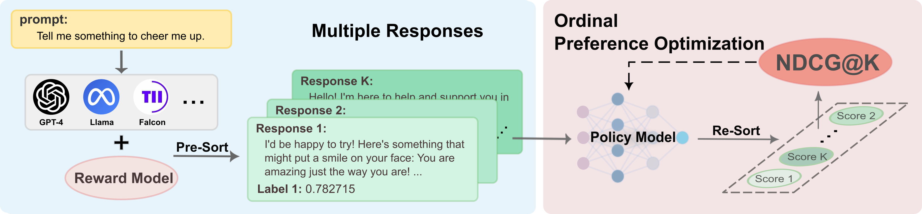
Figure 1: An illustration of Ordinal Preference Optimization (OPO) workflow. Each response is assigned a ground truth label by the reward model and pre-sorted in descending order. Reward scores are then derived from the policy and re-sorted to a new permutation. OPO calculates NDCG@K from the difference between two permutations and optimizes the policy model.

We construct a multiple response dataset assigned with ordinal rewards based on UltraFeedback [9] and SimPO [31]. Comprehensive experiments are conducted to evaluate model performance with various pairwise and listwise benchmarks across different list sizes and hyperparameters. Our method OPO consistently achieves the best performance on both evaluation datasets and general benchmarks like AlpacaEval [26]. We investigate the impact of positive-negative pairs of varying quality on pairwise preference alignment. Our findings reveal that employing a diverse range of negative samples enhances model performance compared to using only the lowest-quality response as negative under the same single positive sample. Moreover, aligning all pairs of listwise responses (i.e., multiple positives against multiple negatives) does not significantly boost performance compared to jointly aligning one positive against multiple negatives. This indicates that a larger pool of negative samples leads to better performance in the pairwise contrastive scenario, as trivial negatives can result in suboptimal outcomes.

Our contributions are summarized as follows:

• We propose a new listwise alignment method named OPO that can leverage ordinal multiple responses, which demonstrates superior performance than existing pairwise and listwise approaches across various model scales.

• We establish a connection between ranking models in information retrieval and the alignment problem in LLMs by illustrating the effectiveness of directly optimizing ranking metrics for LLM alignment.

• We construct an ordinal multiple responses dataset and demonstrate that increasing the pool of negative samples can enhance the performance of existing pairwise approaches.

2 Preliminaries

The traditional RLHF framework aligns large language models (LLMs) with binary human preferences in a contrastive manner, which maximizes the likelihood of the preferred response $y_{w}$ over the non-preferred $y_{l}$. In contrast, this paper adopts the Learning to Rank (LTR) framework, which learns how to permute a list of responses by ranking models.

2.1 Problem Setting

Following the setup in LiPO [29], we assume access to an offline static dataset $\mathcal{D}=\{x^{(i)},\mathbf{Y}^{(i)},\mathbf{\Psi}^{(i)}\}_{i=1}^{N}$, where $\mathbf{Y}=(y_{1},...,y_{K})$ is a list of responses from various generative models of size K given the prompt $x$. Each response is associated with a label from $\mathbf{\Psi}=(\psi_{1},...,\psi_{K})$, also known as the ground truth labels in the Learning to Rank literature. The label $\psi$ measures the quality of responses, which can be generated from human feedback or a pre-trained reward model. In the empirical study, we obtain the score $\mathbf{\Psi}$ from a reward model as

$$\psi_{k}=RM(x,y_{k}),$$ (1)

where $\psi_{k}\in[0,1]$. The label is fixed for a response, representing the degree of human preference.

For each prompt-response pair, we also compute a reward score representing the likelihood of the generating probability of the response:

$$s(x,y)=\beta\log\frac{\pi_{\theta}(y|x)}{\pi_{\text{ref}}(y|x)}.$$ (2)

Here, $\pi_{\text{ref}}$ is a reference model which we set as the SFT model. $\pi_{\theta}(y|x)$ and $\pi_{\text{ref}}(y|x)$ means the probability of the response $y$ given the prompt $x$ under the policy model and the reference model. Similar to DPO [38], the partition function is omitted due to the symmetry in the choice model of multiple responses. Unlike the fixed labels $\psi_{k}$, the reward scores $\mathbf{s}=\{s(x,y_{1}),...,s(x,y_{K})\}$ depend on the model $\pi_{\theta}$ and are updated during the model training.

2.2 NDCG Metric

Normalized Discounted Cumulative Gain (NDCG) [6, 19] is a widely-used metric for evaluating the ranking model performance, which directly assesses the quality of a permutation from listwise data. Assume the list of responses $\mathbf{Y}=(y_{1},...,y_{K})$ have been pre-ranked in the descending order based on labels $\mathbf{\Psi}=(\psi_{1},...,\psi_{K})$ from Eq 1, where $\psi_{i}\geq\psi_{j}$ if $i\geq j$. The Discounted Cumulative Gain at k-th position ($k\leq K$) is defined as:

$$\text{DCG@}k=\sum_{j=1}^{k}G(\psi_{j})D(\tau(j)),$$ (3)

where $\psi_{j}$ denotes the ground truth labels of the response $y_{j}$, and $\tau(j)$ is the descending rank position of $y_{j}$ based on the reward scores $\mathbf{s}$ computed by the current model $\pi_{\theta}$. Typically, the discount function and the gain function are set as $D(\tau(j))=\frac{1}{\log_{2}(\tau(j)+1)}$ and $G(\psi_{j})=2^{\psi_{j}}-1$. An illustration is provided in Appendix A.1.

The NDCG at k is defined as

$$\text{NDCG@}k=\frac{1}{\text{maxDCG@}k}\text{DCG@}k,$$ (4)

where $\text{maxDCG@}k$ is the maximum possible value of $\text{DCG@}k$, computed by ordering the responses $\mathbf{Y}$ by their ground truth labels $\mathbf{\Psi}$. The normalization ensures that NDCG is within the range (0, 1).

The value $k$ of NDCG@$k$ ($k\leq K$) indicates that we focus on the ranking of the top $k$ elements while ignoring those beyond $k$. For example, when $k=2$, we only need to correctly order the first 2 elements, regardless of the order of the remaining $K-2$ elements in the list. It means solely making $s_{1}\geq s_{2}$ (because $\psi_{1}\geq\psi_{2}$ always holds) leads to the maximum NDCG@2 value.

3 Ordinal Preference Optimization

In LLM alignment, the reward score $\mathbf{s}$ in Eq 2 is the key component connecting the loss objective to model parameters $\theta$. However, there is a gap between using NDCG as an evaluation metric and a training objective, since the NDCG metric is non-differentiable with respect to reward scores $\mathbf{s}$, which prevents the utilization of gradient descent to optimize models.

To overcome this limitation, surrogate losses [48] have been developed. These losses approximate the NDCG value by converting its discrete and non-differentiable characteristics into a continuous and score-differentiable form, suitable for backpropagation. The original NDCG is computed by iterating over each list element’s gain value and multiplying it by its corresponding position discount, a process known as the alignment between gains and discounts (i.e., each gain is paired with its respective discount). Thus, surrogate losses can be interpreted in two parts: aligning gains and discounts to approximate the NDCG value, and ensuring these functions are differentiable with respect to the score to enable gradient descent optimization. We will leverage NeuralNDCG as such a surrogate loss [36].

3.1 NeuralSort relaxation

NeuralNDCG incorporates a score-differentiable sorting algorithm to align gain values $G(\cdot)$ with position discounts $D(\cdot)$. This sorting operation is achieved by left-multiplying a permutation matrix $P_{\text{sort}(\mathbf{s})}$ with the score vector $\mathbf{s}$ to obtain a list of scores sorted in descending order. The element $P_{\text{sort}(\mathbf{s})}[i,j]$ denotes the probability that response $y_{j}$ is ranked in the $i$-th position after re-sorting based on $\mathbf{s}$. Applying this matrix to the gains $G(\cdot)$ results in the sorted gains vector $\widehat{G(\cdot)}$, which is aligned with the position discounts. For detailed illustrations, please refer to Appendix A.1.

To approximate the sorting operator, we need to approximate this permutation matrix. In NeuralSort [16], the permutation matrix is approximated using a unimodal row stochastic matrix $\widehat{P}_{\text{sort}(\mathbf{s})}(\tau)$, defined as:

$$\widehat{P}_{\text{sort}(\mathbf{s})}[i,:](\tau)=\text{softmax}\left[\frac{((n+1-2i)\mathbf{s}-A_{\mathbf{s}}\mathbf{1})}{\tau}\right].$$ (5)

Here, $A_{\mathbf{s}}$ is the matrix of absolute pairwise differences of elements in $\mathbf{s}$, where $A_{\mathbf{s}}[i,j]=|s_{i}-s_{j}|$, and $\mathbf{1}$ is a column vector of ones. The row of $\widehat{P}_{\text{sort}(\mathbf{s})}$ always sums to one. The temperature parameter $\tau>0$ controls the accuracy of the approximation. Lower values of $\tau$ yield better approximations but increase gradient variance. It can be shown that:

$$\lim_{\tau\to 0}\widehat{P}_{\text{sort}(\mathbf{s})}(\tau)=P_{\text{sort}(\mathbf{s})}.$$ (6)

A more specific simulation is shown in Table 6. For simplicity, we refer to $\widehat{P}_{\text{sort}(\mathbf{s})}(\tau)$ as $\widehat{P}$.

3.2 OPO Objective with NeuralNDCG

Similar to the original NDCG, but with the gain function $G(\cdot)$ replaced by $\widehat{G(\cdot)}=\widehat{P}\cdot G(\cdot)$ to ensure proper alignment between gains and discounts. The estimated gain at rank $j$ can be interpreted as a weighted sum of all gains, where the weights are given by the entries in the $j$-th row of $\widehat{P}$. Since $\widehat{P}$ is a row-stochastic matrix, each row sums to one, though the columns may not. This can cause $\widehat{G}$ to disproportionately influence the NDCG value at certain positions. To address this issue, Sinkhorn scaling [41] is employed on $\widehat{P}$ to ensure each column sums to one. Then we get the NeuralNDCG [36] formula:

$$\text{NeuralNDCG@}k\ (\tau;\mathbf{s},\mathbf{\Psi})=N_{k}^{-1}\sum_{j=1}^{k}(\text{scale}(\widehat{P})\cdot G(\mathbf{\Psi}))_{j}\cdot D(j),$$ (7)

where $N_{k}^{-1}$ represents the $\text{maxDCG@}k$ (for $k\leq K$) as defined in Equation 4. The function $\text{scale}(\cdot)$ denotes Sinkhorn scaling, and $G(\cdot)$ and $D(\cdot)$ are the gain and discount functions, respectively, as in Equation 3. Intuitively, the gain function should be proportional to the label, effectively capturing the relative ranking of different responses. The discount function penalizes responses appearing later in the sequence, as in many generation or recommendation tasks the focus is on the top-ranked elements, especially the first. Thus, higher-ranked responses have a more significant impact on the overall loss in NeuralNDCG. Further illustrations are provided in Appendix A.1.

Finally, we derive the OPO objective, which can be optimized using gradient descent:

$$\mathcal{L}_{\text{NeuralNDCG@k}}(\pi_{\theta};\pi_{\text{ref}})=-\mathbb{E}_{(x,\mathbf{Y},\mathbf{\Psi})\sim\mathcal{D}}\left[N_{k}^{-1}\sum_{j=1}^{k}(\text{scale}(\widehat{P})\cdot G(\mathbf{\Psi}))_{j}\cdot D(j)\right].$$ (8)

Note that setting $k=2$ with $K>2$ is not equivalent to having a list size of $K=2$. The former indicates a focus on the top-2 responses from the entire list, where a higher rank signifies superior response quality. Conversely, $K=2$ typically refers to a binary contrastive scenario, classifying responses as positive or negative samples and maximizing the likelihood of preferred response $y_{w}$ over non-preferred $y_{l}$. In high-quality response pairs, labeling one as negative may adversely impact the generation quality of LLMs. OPO provides a more comprehensive view of relative proximities within multiple ordinal responses. In this work, we set $k=K$ by default.

3.3 Other Approximation of NDCG

In addition to aligning gains and discounts, we can modify the discount function to be differentiable. ApproxNDCG [37] is proposed as an approximation to the rank position in the NDCG equation (Eq 3) using the sigmoid function:

$$\widehat{\tau(j)}=1+\sum_{i\neq j}\frac{\exp{(-\alpha(s_{j}-s_{i}))}}{1+\exp{(-\alpha(s_{j}-s_{i}))}}=1+\sum_{i\neq j}\sigma(\alpha(s_{i}-s_{j})).$$ (9)

As observed, if $s_{i}\gg s_{j}$, the descending rank position of $y_{j}$ will increase by $1$. Note that the hyperparameter $\alpha$ controls the precision of the approximation. We then obtain the estimated $\widehat{\tau(j)}$ and subsequently the ApproxNDCG objective:

$$\mathcal{L}_{\text{ApproxNDCG@k}}(\pi_{\theta};\pi_{\text{ref}})=-\mathbb{E}_{(x,\mathbf{Y},\mathbf{\Psi})\sim\mathcal{D}}\left[N_{k}^{-1}\sum_{j=1}^{k}G(\psi_{j})\cdot D(\widehat{\tau(j)})\right].$$ (10)

4 Experiments

Our empirical studies address two critical questions: Q1: Can we employ ranking metrics as training objectives in LLM alignment problem? Q2: How does selecting different pairs on multi-response data impact the performance of DPO? For Q1, we demonstrate that OPO outperforms other baselines across various evaluation benchmarks. To answer Q2, we compare three pairwise paradigms of DPO on multi-response data. Our findings show that increasing the pool of negative samples can enhance model performance by mitigating the effects of trivial negatives.

Baselines To explore the connection between LLM alignment and ranking tasks, as well as the performance of OPO, we employ various pairwise and listwise alignment baselines. Their optimization objectives are detailed in Table 1. We introduce three paradigms of positive-negative pairs for DPO on ordinal multiple responses. LiPO-$\lambda$ [29] incorporates LambdaRank from the Learning to Rank (LTR) literature, acting as a weighted version of DPO. SLiC and RRHF employ a similar hinge contrastive loss. ListMLE utilizes the Plackett-Luce Model [35] to represent the likelihood of list permutations. For further information, please see Appendix A.2.

Datasets We construct a multi-response dataset named ListUltraFeedback. This dataset combines four responses from UltraFeedback and five generated responses from the fine-tuned Llama3-8B model in SimPO [9, 31], all based on the same prompts. All responses are assigned ordinal ground truth labels using the Reward Model ArmoRM [50]. This model is the leading open-source reward model, outperforming both GPT-4 Turbo and GPT-4o in RewardBench [25] at the time of our experiments. To ensure clear distinction between positive and negative samples, while maintaining diversity, we select two responses with the highest scores and two with the lowest. Additionally, we randomly draw four responses from the remaining pool. Details of the dataset are presented in Table 2.

Training Details We select Qwen2-0.5B [1] and Mistral-7B [20] as our foundation models, representing different parameter scales. Following the training pipeline in DPO [38], Zephyr [46], and SimPO [31], we start with supervised fine-tuning (SFT) [1] on UltraChat-200k [10] to obtain our SFT model. We then apply various pairwise and listwise approaches to align preferences on our ordinal multiple response dataset, ListUltraFeedback. Adhering to the settings in HuggingFace Alignment Handbook [45], we use a learning rate of $5\times 10^{-7}$ and a total batch size of 128 for all training processes. The models are trained using the AdamW optimizer [23] on 4 Nvidia V100-32G GPUs for Qwen2-0.5B models and 16 Nvidia V100-32G GPUs for Mistral-7B. Unless noted otherwise, we fix $\alpha=25$ for ApproxNDCG and $\tau=1$ for OPO to achieve optimal performance, as determined by ablation studies and hyperparameter sensitivity analysis presented in Section 4.2. Both models and datasets are open-sourced, ensuring high transparency and ease of reproduction. Further training details can be found in Appendix A.3.

Method	Type	Objective
DPO - Single Pair (13)	Pairwise	$-\log\sigma\left(s_{1}-s_{K}\right)$
DPO - BPR (14)	Pairwise	$-\frac{1}{K-1}\sum_{j\neq 1}^{K}\log\sigma\left(s_{1}-s_{j}\right)$
DPO - All Pairs (15)	Pairwise	$-\binom{K}{2}^{-1}\sum_{\psi_{i}>\psi_{j}}\log\sigma\left(s_{i}-s_{j}\right)$
LambdaRank (16)	Pairwise	$-\binom{K}{2}^{-1}\sum_{\psi_{i}>\psi_{j}}\Delta_{i,j}\log\sigma\left(s_{i}-s_{j}\right)$
		where $\Delta_{i,j}=|G_{i}-G_{j}|\cdot\left|{D(\tau(i))}-{D(\tau(j))}\right|$
SLiC (17)	Pairwise	$-\binom{K}{2}^{-1}\sum_{\psi_{i}>\psi_{j}}\max(0,1-(s_{i}-s_{j}))$
ListMLE (18)	Listwise	$-\log\prod_{k=1}^{K}\frac{exp(s_{k})}{\sum_{j=k}^{K}exp(s_{j})}$
ApproxNDCG (10)	Listwise	$-N_{k}^{-1}\sum_{j=1}^{k}G(\psi_{j})\cdot D(\widehat{\tau(j)})$
OPO (8)	Listwise	$-N_{k}^{-1}\sum_{j=1}^{k}(\text{scale}(\widehat{P})\cdot G(\mathbf{\Psi}))_{j}\cdot D(j)$

Table 1: Pairwise and listwise baselines given ordinal multiple-response data $\mathcal{D}=(x,\mathbf{Y},\mathbf{\Psi})$.

Evaluation The KL-divergence in the original RLHF pipeline is designed to prevent the Policy model from diverging excessively from the SFT model, thus avoiding potential manipulation of the Reward Model. As we employ ArmoRM in the construction of the training dataset,we incorporate various judging models and evaluation benchmarks, such as different Reward models and AlpacaEval [26] with GPT-4, to reduce the impact of overfitting on ArmoRM. We design 2 pipelines to thoroughly analyze the performance of OPO, using the Win Rate of generated responses from aligned models compared to the SFT model as our primary metric. Details of evaluation datasets are presented in Table 2.

In the Proxy Model pipeline, we deploy the Scoring Reward Model ArmoRM [50] and the Pair-Preference Reward Model [12] as Proxy Models to calculate the win rate on ListUltraFeedback. Both Proxy models surpass GPT-4 Turbo and GPT-4o in rewarding tasks on RewardBench [25]. The Scoring model provides a score in the range $(0,1)$ for a given prompt and response, while the Pair-Preference model outputs the winner when given a prompt and two responses, offering a more intuitive approach for pairwise comparisons.

In the General Benchmark pipeline, we evaluate our models using two widely recognized benchmarks: AlpacaEval [26] and MT-Bench [59], which assess the model’s comprehensive conversational abilities across various questions. Consistent with the original setup, we employ GPT-4 Turbo [2] as the standard judge model to determine which of the two responses exhibits higher quality.

Datasets	Examples	Judge Model	Notes
UltraChat200k	208k	-	SFT
ListUltraFeedback${}_{\text{train}}$	59.9k	-	Ordinal Preference Optimization
ListUltraFeedback${}_{\text{test}}$	1968	RLHFlow Pair-Preference	Pair-Preference win rates
		ArmoRM	Scoring win rates
AlpacaEval	805	GPT-4 Turbo	Pair-Preference win rates
MT-Bench	80	GPT-4 Turbo	Scoring win rates

Table 2: Details of training datasets and evaluation datasets.

4.1 Main Results

We list win rates of various alignment approaches across diverse evaluation benchmarks in Table 3. Pairwise contrastive methods that leverage extensive structural information from multiple responses outperform those relying solely on traditional single pairs. Both BPR and All Pairs methods exceed the performance of Single Pair, with no significant difference between BPR and All Pairs, particularly evident with the Mistral-7B model (Table 5). This suggests that utilizing diverse negative samples is more crucial than varying positive samples in pairwise contrastive scenarios. Trivial negatives lead to suboptimal outcomes, but a larger pool of negative samples can reduce the uncertainty associated with their varying quality.

When the list size is 8, the OPO algorithm, which directly optimizes an approximation of NDCG, achieves superior performance. OPO’s advantage over pairwise and ListMLE methods lies in its ability to effectively utilize the relative proximities within ordinal multiple responses. Traditional contrastive pairwise approaches tend to crudely classify one response as negative and maximize the likelihood of the preferred response $y_{w}$ over the non-preferred $y_{l}$. It can adversely affect the generation quality of LLMs when high-quality responses are treated as negative samples. In contrast, OPO provides a more nuanced approach to handling the relationships between responses.

Method	Type	Proxy Model		General Benchmark
		Pair-Preference	Scoring	AlpacaEval	MT-Bench
Single Pair	Pairwise	60.75	56.86	57.95	52.81
BPR	Pairwise	60.32	58.33	58.74	55.00
All Pairs	Pairwise	63.82	60.54	57.23	53.13
SLiC	Pairwise	63.31	60.70	61.00	53.75
LambdaRank	Pairwise	62.30	59.04	58.72	55.31
ListMLE	Listwise	63.03	59.76	57.05	53.13
ApproxNDCG	Listwise	61.46	58.59	58.16	55.94
OPO	Listwise	64.25	61.36	61.64	53.44

Table 3: The proposed OPO and ApproxNDCG outperform existing baselines across various evaluation benchmarks. The win rates are derived from comparisons between the preference-aligned Qwen2-0.5B and its SFT model. We fix $\alpha=25$ for ApproxNDCG and $\tau=1$ for OPO. We also set $\beta=0.1$ in Eq 2 for all methods except $\beta=0.05$ for SLiC to achieve the optimal performance.

4.2 Ablation Study

Score Function Scale The hyperparameter $\beta$ controls the scaling of the score function Eq 2 and the deviation from the base reference policy $\pi_{\text{ref}}$, which is significantly influence models performance. Following the common setting in previous works [38, 31, 29], we set the hyperparameter space of $\beta$ as $[0.01,0.05,0.1,0.5]$ and conduct sensitivity analysis over broad approaches. As illustrated in Fig 2, all methods achieve their best performance at $\beta=0.1$ except the SLiC method. OPO consistently achieves the best performance on both $\beta=0.05$ and $\beta=0.1$. More detailed results are shown in Table 8.

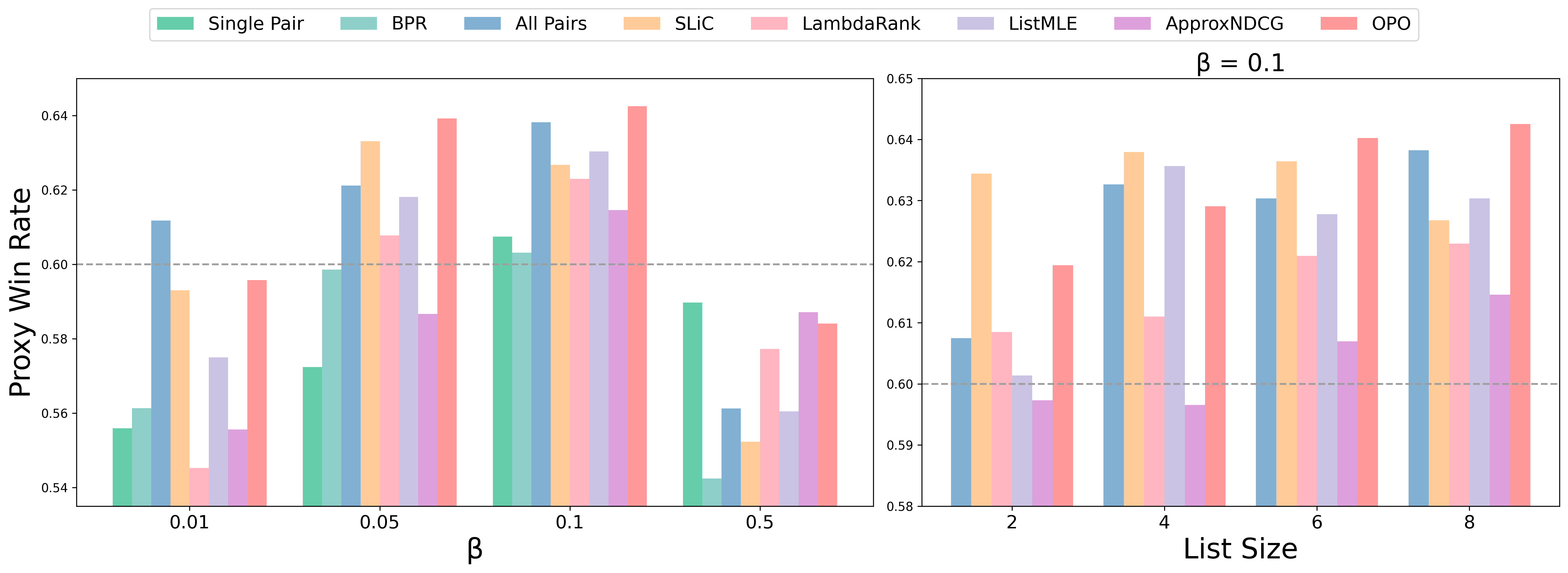
Figure 2: OPO outperforms other methods across different $\beta$ and list sizes. The Proxy win rates are calculated by Pair-Preference Proxy model by comparing preference-aligned Qwen2-0.5B against its SFT model.

List Size To evaluate the effectiveness of listwise methods in leveraging the sequential structure of multiple responses compared to pairwise methods, we analyze performance across varying list sizes. The results, presented in Figure 2, indicate that models trained with multiple responses (more than two) significantly outperform those using binary responses. Many models achieve optimal performance with a list size of 8. Notably, the OPO method (Equation 7) consistently outperforms other approaches when $K>4$, with performance improving as list size increases. This trend is also evident across different values of $\beta$, as shown in the supplementary results 9.

Approximation Accuracy The temperature parameter $\tau$ controls the approximation accuracy and gradient variance of NeuralNDCG [36]. We visualize the values of NDCG and NeuralNDCG on specific data and assess model performance with various $\tau$. The results, shown in Figure 3, reveal that as NeuralNDCG more closely approximates true NDCG, model performance tends to decline. This may occur because training involves multiple high-quality responses with similar ground truth labels. Enforcing responses to conform to NDCG’s step-wise structure can reduce the likelihood of these good responses. Additionally, as the approximation accuracy of NeuralNDCG increases, more plateaus appear due to NDCG’s inherent step-wise nature. On these plateaus, gradients become zero, preventing model optimization on these data points. A similar observation is confirmed in ApproxNDCG, as discussed in Appendix A.5.

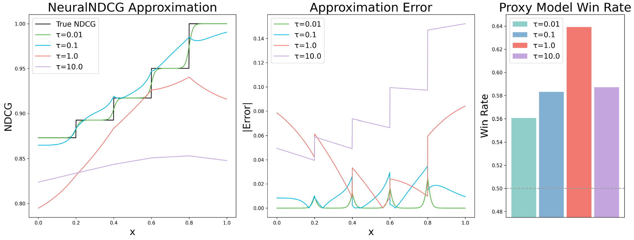
Figure 3: Higher NDCG approximation accuracy doesn’t always lead to better performance. Given ground truth label $\psi=[1.0,0.8,0.6,0.4,0.2]$ and the scores $\mathbf{s}=[x,0.8,0.6,0.4,0.2]$, an illustration of NeuralNDCG Approximation Accuracy with different $\tau$ and its corresponding absolute value of error and Pair-Preference Proxy model win rates against SFT.

OPO Setup We set $\tau=1.0$ and perform an ablation study on key components of OPO, with results shown in Table 4. (i) When evaluating the NDCG@4 metric (Equation 7) for multiple responses with a list size of 8, the performance is comparable to OPO with a list size of 4. This suggests that OPO’s effectiveness is more influenced by the quantity and size of listwise data rather than the specific metric calculation method. (ii) The choice of gain function, whether $G_{i}=2^{\psi_{i}}-1$ or $G_{i}=\psi_{i}$, does not significantly impact model performance. The critical factor is that the gain function provides the correct ranking order and reflects the relative proximity of different responses. (iii) Omitting Sinkhorn scaling [41] on $\widehat{P}$ significantly degrades performance. Without scaling, the permutation matrix $\widehat{P}$ may not be column-stochastic, meaning each column may not sum to one. This can cause the weighted sum of $G(\cdot)$ to disproportionately contribute to the estimated gain function $\widehat{G(\cdot)}$ (Equation 7), thereby adversely affecting results.

Method	$\beta$	Pair-Preference	Scoring	$\beta$	Pair-Preference	Scoring
All Pairs	0.1	63.82	60.54	0.05	62.12	58.36
OPO	0.1	64.25	61.36	0.05	63.92	60.09
Top-4	0.1	61.92	59.35	0.05	61.36	58.64
w/o Power	0.1	63.49	61.28	0.05	64.05	59.45
w/o Scale	0.1	57.32	56.20	0.05	57.49	55.72

Table 4: Ablation study results for OPO Setup on Qwen2-0.5B: (i) Only calculate the top-4 NDCG metric; (ii) Replace the exponential function with the direct label as the gain function; (iii) Remove the Sinkorn Scale function in Eq 8.

Model Scale Up To thoroughly assess the performance of OPO, we employ the Mistral-7B model [20] as our large-scale language model. Following the SimPO pipeline [31], we use Zephyr-7B-SFT from HuggingFace [46] as the SFT model. Mistral-7B is then aligned with ordinal multiple preferences on ListUltraFeedback, and its performance is validated across evaluation sets and standard benchmarks, as shown in Table 5. For hyperparameter details and additional results, refer to Appendix A.3 and A.4.2.

Method	Type	Proxy Model		General Benchmark		Avg.
		Pair-Preference	Scoring	AlpacaEval	MT-Bench
Single Pair	Pairwise	71.90	70.66	74.75	52.19	67.38
BPR	Pairwise	84.43	82.37	86.69	63.44	79.23
All Pairs	Pairwise	85.34	83.31	82.79	61.56	78.25
SLiC	Pairwise	84.12	83.46	83.27	66.25	79.28
LambdaRank	Pairwise	85.11	82.52	86.13	69.06	80.71
ListMLE	Listwise	83.79	83.61	83.46	66.56	79.35
ApproxNDCG	Listwise	82.04	74.64	85.80	67.50	77.50
OPO	Listwise	84.98	83.05	87.54	67.81	80.85

Table 5: OPO outperforms other baselines on win rates of aligned Mistral-7B against Zephyr-7B-SFT. We set $\beta=0.01$ for Single Pair and $\beta=0.05$ for other approaches to achieve the best performance. The other settings are the same as in Table 3.

OPO demonstrates competitive performance on win rates against the SFT model. To clearly illustrate OPO’s advantages over other methods, we compare their generated responses and present OPO’s win rates in Figure 4. More detailed comparisons can be found in Figure 5.

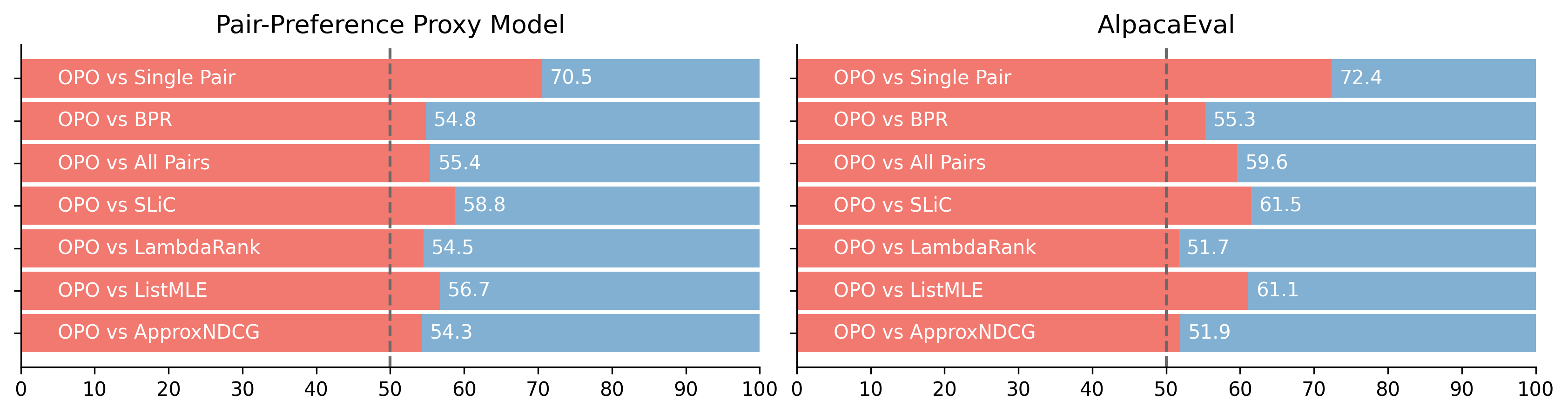
Figure 4: OPO outperforms other approaches on direct comparisons with Mistral-7B. The win rates are derived from comparisons between OPO and other methods on their optimal settings. We employ the Pair-Preference Proxy model on evaluation sets and GPT-4 on AlpacaEval as the judge models.

5 Related Work

Pairwise Preference Optimization Direct Preference Optimization (DPO) [38] removes the necessity for an explicit reward model within the RLHF framework by introducing a novel algorithm to compute reward scores for each response. Similar to RLHF, DPO uses the Bradley-Terry (BT) model [5] to align binary human preferences in a contrastive manner. Subsequent research, including methods like IPO, KTO, RPO, SimPO, and others [28, 54, 3, 55, 15, 18, 34, 31], focus on refining the reward function and the BT model to enhance performance and simplify the process. Additionally, iterative methods are developed to align pairwise preferences with a dynamic reference model [40, 33, 22, 56]. They classify preferred responses $y_{w}$ as positive samples and non-preferred responses $y_{l}$ as negative samples, with the objective of maximizing the likelihood of $r(x,y_{w})$ over $r(x,y_{l})$. These contrastive techniques are influenced by the quality and quantity of negative samples. As indicated by the contrastive learning literature, the presence of hard negatives and large batch size is crucial [7]. Incorporating trivial negatives can lead to suboptimal results; hence, leveraging multiple-response data can expand the pool of candidate samples, reducing the likelihood of trivial negatives.

Multiple Responses Alignment Recent research has introduced simple and efficient methods to align human preferences across multiple responses. These approaches expand candidate responses from various large language models (LLMs) such as ChatGPT, Alpaca, and GPT-4, assigning ordinal rewards via reward models or human feedback. RRHF[57] employs the same hinge objective as SLiC [58] on ordinal multiple responses through pairwise comparisons. LiPO-$\lambda$ [29] incorporates LambdaRank [13] where higher-quality responses against lower-quality ones receive greater weights, acting as a weighted version of DPO. However, when handling high-quality response pairs, incorrectly classifying one of them as the negative sample and minimizing its likelihood can adversely affect LLM generation quality. Listwise methods offer a more nuanced approach to handling relationships between responses. DPO-PL [38] and PRO [42] employ the same PL framework [35] but differ in their reward functions. LIRE [60] calculates softmax probabilities with a consistent denominator and multiplies them by corresponding rewards, functioning as a pointwise algorithm since permutations do not alter loss values. Despite their potential, current listwise techniques are not yet state-of-the-art in the learning-to-rank (LTR) literature, indicating a need for further research.

Learning to Rank Learning to Rank (LTR) involves a set of machine learning techniques widely applied in information retrieval, web search, and recommender systems [30, 21, 17, 27]. The goal is to train a ranking model by learning a scoring function $s=f(x,y)$ that assigns scores to elements for ranking purposes. The loss is computed by comparing the current permutation with the ground truth, which updates the model parameters $\theta$. Loss functions in LTR are generally categorized into three types: pointwise, pairwise, and listwise. Pointwise and pairwise methods convert the ranking task into classification problems, often overlooking the inherent structure of ordered data. Conversely, listwise approaches [53] directly tackle the ranking problem by considering entire ranking lists as training instances. This approach fully exploits the relative proximities within ordinal multiple responses, providing a more comprehensive understanding of the ranking relationships.

6 Discussion

In this work, we propose Ordinal Preference Optimization (OPO), a novel listwise preference optimization algorithm to align ordinal human preferences. By optimizing the standard ranking metric NDCG, OPO learns a score function that assigns reward scores to responses and ranks them properly, and it connects ranking models in information retrieval and LLM alignment. Empirical studies show that OPO consistently outperforms existing pairwise and listwise approaches across various training setups and evaluation benchmarks.

Our study has several limitations and suggests promising directions for future research. In constructing ordinal multiple responses, a pre-trained Reward Model serves as the judge model, which might not fully align with real-world human preferences. Future study can develope more robust and secure data construction methods to ensure responses remain harmless and improve model alignment quality. Additionally, there is a lack of theoretical analysis on aligning human preferences as a Learning to Rank (LTR) task despite its empirical success. The extensive LTR literature remains underexplored, indicating potential for further research and applications in related fields.

Appendix A Appendix

A.1 Illustration of Sorting Operations

Given the input ground truth labels $\mathbf{\Psi}=[5,4,3,2]^{T}$ and scores $\mathbf{s}=[9,1,5,2]^{T}$, the descending order of $\mathbf{\Psi}$ based on the current reward scores $\mathbf{s}$ is $\mathbf{\tau}=[1,4,2,3]^{T}$. According to the formula introduced in Eq 3:

$$\text{DCG@4}=\sum_{j=1}^{k}G(\psi_{j})\cdot D(\tau(j))=\frac{G(5)}{\log_{2}(1+1)}+\frac{G(4)}{\log_{2}(1+4)}+\frac{G(3)}{\log_{2}(1+2)}+\frac{G(2)}{\log_{2}(1+3)}$$

Building upon the preliminaries defined in [16], consider an $n$-dimensional permutation $\mathbf{z}=[z_{1},z_{2},\ldots,z_{n}]^{T}$, which is a list of unique indices from the set ${1,2,\ldots,n}$. Each permutation $\mathbf{z}$ has a corresponding permutation matrix $P_{\mathbf{z}}\in{0,1}^{n\times n}$, with entries defined as follows:

$$P_{\mathbf{z}}[i,j]=\begin{cases}1&\text{if }j=z_{i}\\ 0&\text{otherwise}.\end{cases}$$ (11)

Let $\mathbb{Z}_{n}$ denote the set containing all $n!$ possible permutations within the symmetric group. We define the $\text{sort}:\mathbb{R}^{n}\rightarrow\mathbb{Z}_{n}$ operator as a function that maps $n$ real-valued inputs to a permutation representing these inputs in descending order.

The $\text{sort}(\mathbf{s})=[1,3,4,2]^{T}$ since the largest element is at the first index, the second largest element is at the third index, and so on. We can obtain the sorted vector simply via $P_{\text{sort}(\mathbf{s})}\cdot\mathbf{s}$:

$$P_{\text{sort}(\mathbf{s})}\cdot\mathbf{s}=\begin{pmatrix}1&0&0&0\\ 0&0&1&0\\ 0&0&0&1\\ 0&1&0&0\\ \end{pmatrix}\begin{pmatrix}9\\ 1\\ 5\\ 2\\ \end{pmatrix}=\begin{pmatrix}9\\ 5\\ 2\\ 1\\ \end{pmatrix}$$ (12)

Here we demonstrate the results by conducting NeuralSort Relaxation Eq 5 with different $\tau$.

	$\widehat{P_{\text{sort}(\mathbf{s})}}\cdot\mathbf{s}$
$\lim_{\tau\to 0}$	9	5	2	1
$\tau=0.01$	9.0000	5.0000	2.0000	1.0000
$\tau=0.1$	9.0000	5.0000	2.0000	1.0000
$\tau=1.0$	8.9282	4.9420	1.8604	1.2643
$\tau=10.0$	6.6862	4.8452	3.2129	2.2557

Table 6: Illustration of Sorting Operation of ground truth labels $\mathbf{\Psi}=[5,4,3,2]^{T}$ and scores $\mathbf{s}=[9,1,5,2]^{T}$ via NeuralSort [16] with different $\tau$.

When we integrate the NeuralNDCG formula in Eq 7, ideally, $\lim_{\tau\to 0}\widehat{P}_{\text{sort}(\mathbf{s})}(\tau)=P_{\text{sort}(\mathbf{s})}$, yielding the following result:

$$\widehat{G}=P_{\text{sort}(\mathbf{s})}\cdot\text{G}(\mathbf{\Psi})=\begin{pmatrix}1&0&0&0\\ 0&0&1&0\\ 0&0&0&1\\ 0&1&0&0\\ \end{pmatrix}\begin{pmatrix}\text{G(5)}\\ \text{G(4)}\\ \text{G(3)}\\ \text{G(2)}\\ \end{pmatrix}=\begin{pmatrix}\text{G(5)}\\ \text{G(3)}\\ \text{G(2)}\\ \text{G(4)}\\ \end{pmatrix}$$

Then,

$$\text{NeuralDCG@4}=\sum_{j=1}^{k}(\widehat{G})_{j}\cdot D(j)=\frac{G(5)}{\log_{2}(1+1)}+\frac{G(3)}{\log_{2}(1+2)}+\frac{G(2)}{\log_{2}(1+3)}+\frac{G(4)}{\log_{2}(1+4)}$$

which can be easily seen to be the same as DCG@4 as long as we keep the alignment between gains and discounts.

A.2 Details of Baselines

Table 1 shows the types and objectives of the baselines we consider in the empirical study.

To ensure variable consistency and comparability of experiments, we choose the original DPO algorithm as our reward score function Eq 2 and pairwise baseline method and assess its performance in both binary-response and multi-response scenarios.

DPO-BT In detail, we implement three variants of the original sigmoid-based pairwise DPO based on the Bradley-Terry (BT) methods while aligning multiple responses. The first one is Single Pair paradigm, where we compare only the highest-scoring and lowest-scoring responses, which is equivalent to the original DPO in the pairwise dataset scenario.

$$\mathcal{L}_{\text{Single Pair}}(\pi_{\theta};\pi_{\text{ref}})=-\mathbb{E}_{(x,\mathbf{Y},\mathbf{\Psi})\sim\mathcal{D}}\left[\log\sigma\left(s_{1}-s_{K}\right)\right],$$ (13)

Then we introduce the Bayesian Personalized Ranking (BPR) [39] algorithm that computes the response with the highest score against all other negative responses based on Bayes’ theorem, which is widely used in recommender system [17].

$$\mathcal{L}_{\text{BPR}}(\pi_{\theta};\pi_{\text{ref}})=-\mathbb{E}_{(x,\mathbf{Y},\mathbf{\Psi})\sim\mathcal{D}}\left[\frac{1}{K-1}\sum_{j\neq 1}^{K}\log\sigma\left(s_{1}-s_{j}\right)\right],$$ (14)

In the last BT variant, we consider all pairs that can be formed from K responses, which is similar to PRO [42]. This approach allows the model to gain more comprehensive information than the aforementioned methods, including preference differences among intermediate responses, which is referred to as All Pairs:

$$\mathcal{L}_{\text{All Pairs}}(\pi_{\theta};\pi_{\text{ref}})=-\mathbb{E}_{(x,\mathbf{Y},\mathbf{\Psi})\sim\mathcal{D}}\left[\frac{1}{\binom{K}{2}}\sum_{\psi_{i}>\psi_{j}}\log\sigma\left(s_{i}-s_{j}\right)\right],$$ (15)

where $\binom{K}{2}$ denotes the number of combinations choosing 2 out of K elements.

LiPO-$\lambda$ Deriving from the LambdaRank [13], the objective of LiPO-$\lambda$ [29] can be written as follows:

$$\mathcal{L}_{\text{LambdaRank}}(\pi_{\theta};\pi_{\text{ref}},\beta)=-\mathbb{E}_{(x,\mathbf{Y},\mathbf{\Psi})\sim\mathcal{D}}\left[\frac{1}{\binom{K}{2}}\sum_{\psi_{i}>\psi_{j}}\Delta_{i,j}\log\sigma\left(s_{i}-s_{j}\right)\right],$$ (16)

$$\text{where}\quad\Delta_{i,j}=|G_{i}-G_{j}|\cdot\left|{D(\tau(i))}-{D(\tau(j))}\right|.$$

$\Delta_{i,j}$ is referred to as the Lambda weight and $G(\cdot)$ and $D(\cdot)$ is the same gain and discount function in Eq 3.

SLiC Following the analogous objectives proposed in RRHF [57] and SLiC [58], we integrate the pairwise Hinge loss as one of our baselines:

$$\mathcal{L}_{\text{SLiC}}(\pi_{\theta};\pi_{\text{ref}})=\mathbb{E}_{(x,\mathbf{Y},\mathbf{\Psi})\sim\mathcal{D}}\left[\frac{1}{\binom{K}{2}}\sum_{\psi_{i}>\psi_{j}}\max(0,1-(s_{i}-s_{j}))\right],$$ (17)

DPO-PL The DPO objective can also be derived under the Plackett-Luce Model [35] in a listwise manner, which is equivalent to the ListMLE [52] method:

$$\mathcal{L}_{\text{ListMLE}}(\pi_{\theta};\pi_{\text{ref}})=-\mathbb{E}_{(x,\mathbf{Y},\mathbf{\Psi})\sim\mathcal{D}}\left[\log\prod_{k=1}^{K}\frac{exp(s_{k})}{\sum_{j=k}^{K}exp(s_{j})}\right],$$ (18)

A.3 Training Details

The detailed training hyperparameters of Mistral-7B are shown in Table 7.

Hyperparameters	value
Mini Batch	1
Gradient Accumulation Steps	8
GPUs	16$\times$Nvidia V100-32G
Total Batch Size	128
Learning Rate	5e-7
Epochs	1
Max Prompt Length	512
Max Total Length	1024
Optimizer	AdamW
LR Scheduler	Cosine
Warm up Ratio	0.1
Random Seed	42
$\beta$	0.1
$\tau$ for OPO	1.0
$\alpha$ for ApproxNDCG	25
Sampling Temperature	0
Pair-Preference Proxy Model	RLHFlow Pair-Preference
Scoring Proxy Model	ArmoRM
GPT Judge	GPT-4-Turbo
AlpacaEval Judge	alpaca_eval_gpt4_turbo_fn

Table 7: Training hyperparameters for Mistral-7B.

Since Nvidia v100 is incompatible with the bf16 type, we use fp16 for mixed precision in deepspeed configuration. Notably, as the ListMLE method doesn’t have normalization, it will encounter loss scaling errors with mixed precision settings.

A.4 Supplementary Results

A.4.1 Proxy Models Results

The supplementary results of the Proxy Model Win Rate are shown in Table 8 and Table 9. For OPO, we fix $\tau=1.0$. For ApproxNDCG, we fix $\alpha=25$ because it is the parameter $\alpha\cdot\beta$ that controls the approximation accuracy of the sigmoid function in Eq 9.

Run Name	$\beta$	Pair-Preference	Scoring	$\beta$	Pair-Preference	Scoring
Single Pair	0.05	57.24	54.04	0.01	55.59	51.73
	0.1	60.75	56.86	0.5	58.97	58.16
BPR	0.05	59.86	56.86	0.01	56.13	55.16
	0.1	60.32	58.33	0.5	54.24	55.31
All Pairs	0.05	62.12	58.36	0.01	61.18	56.35
	0.1	63.82	60.54	0.5	56.12	55.77
SLiC	0.05	63.31	60.70	0.01	59.30	55.61
	0.1	62.68	60.34	0.5	55.23	55.44
LambdaRank	0.05	60.77	56.07	0.01	54.52	51.35
	0.1	62.30	59.04	0.5	57.72	56.71
ListMLE	0.05	61.81	57.60	0.01	57.49	55.16
	0.1	63.03	59.76	0.5	56.05	55.77
ApproxNDCG	0.05	58.66	54.34	0.01	55.56	50.76
	0.1	61.46	58.59	0.2	60.04	57.27
	0.5	58.71	57.39	1.0	56.61	56.00
OPO	0.05	63.92	60.09	0.01	59.58	55.46
	0.1	64.25	61.36	0.5	58.41	57.65

Table 8: Supplementary Results across different $\beta$ on Qwen2-0.5B.

Run Name	List Size	Pair-Preference	Scoring	Pair-Preference	Scoring
		$\beta=0.1$		$\beta=0.05$
All Pairs	2	60.75	56.86	57.24	54.04
	4	63.26	60.90	61.59	58.54
	6	63.03	59.50	62.83	57.93
	8	63.82	60.54	62.12	58.36
SLiC	2	63.44	59.07	61.00	57.39
	4	63.79	61.40	64.04	60.54
	6	63.64	61.15	62.01	58.61
	8	62.68	60.34	63.31	60.70
LambdaRank	2	60.85	57.62	59.76	56.02
	4	61.10	58.05	59.88	55.51
	6	62.09	57.72	62.02	56.81
	8	62.30	59.04	60.77	56.07
ListMLE	2	60.14	57.01	57.14	53.53
	4	63.57	61.23	61.94	58.49
	6	62.78	60.92	61.18	57.83
	8	63.03	59.76	61.81	57.60
ApproxNDCG	2	59.73	57.72	61.56	58.26
	4	59.65	56.45	60.11	55.79
	6	60.70	57.32	59.53	56.35
	8	61.46	58.59	58.66	54.34
OPO	2	61.94	58.00	58.69	55.89
	4	62.91	59.96	62.65	58.56
	6	64.02	60.11	61.08	59.43
	8	64.25	61.36	63.92	60.09

Table 9: Supplementary Results across different list sizes on Qwen2-0.5B. In practice, we keep the response with the highest label and the one with the lowest label, then conduct random sampling from the remaining responses.

A.4.2 Supplementary Results for Mistral-7B

We observe that decreasing the hyperparameter $\beta$ may increase the performance when language models scale up to 7B parameters. All methods achieve their best performance with $\beta=0.05$ except for Single Pair with $\beta=0.01$. Our approach OPO consistently achieves the best overall performance, shown in Table 10.

Method	$\beta$	Pair-Preference	Scoring	AlpacaEval
Single Pair	0.1	61.26	70.21	64.45
BPR		79.73	77.59	78.39
All Pairs		79.22	78.43	77.65
SLiC		76.17	75.36	73.04
LambdaRank		80.82	78.53	81.01
ListMLE		78.58	79.22	75.12
ApproxNDCG		76.12	69.21	82.50
OPO		83.13	81.66	81.07
Single Pair	0.05	66.44	65.50	68.87
BPR		84.43	82.37	86.69
All Pairs		85.34	83.31	82.79
SLiC		84.12	83.46	83.27
LambdaRank		85.11	82.52	86.13
ListMLE		83.79	83.61	83.46
ApproxNDCG		82.04	74.64	85.80
OPO		84.98	83.05	87.54
Single Pair	0.01	71.90	70.66	74.75
BPR		77.01	78.46	86.71
All Pairs		72.66	74.09	82.44
OPO		73.17	75.00	84.51

Table 10: Model Scale Up results in Mistral-7B.

To further explore the distribution shift during human preference alignment, we demonstrate the score distribution of all methods of which scores are assigned by the Reward model ArmoRM [50] in Fig 5. The OPO method causes the reward score distribution to shift more significantly to the right, resulting in fewer instances at lower scores. Consequently, when compared to the SFT model, its win rate is not as high as methods like All Pairs, SLiC, and ListMLE. However, it can outperform these methods in direct comparisons.

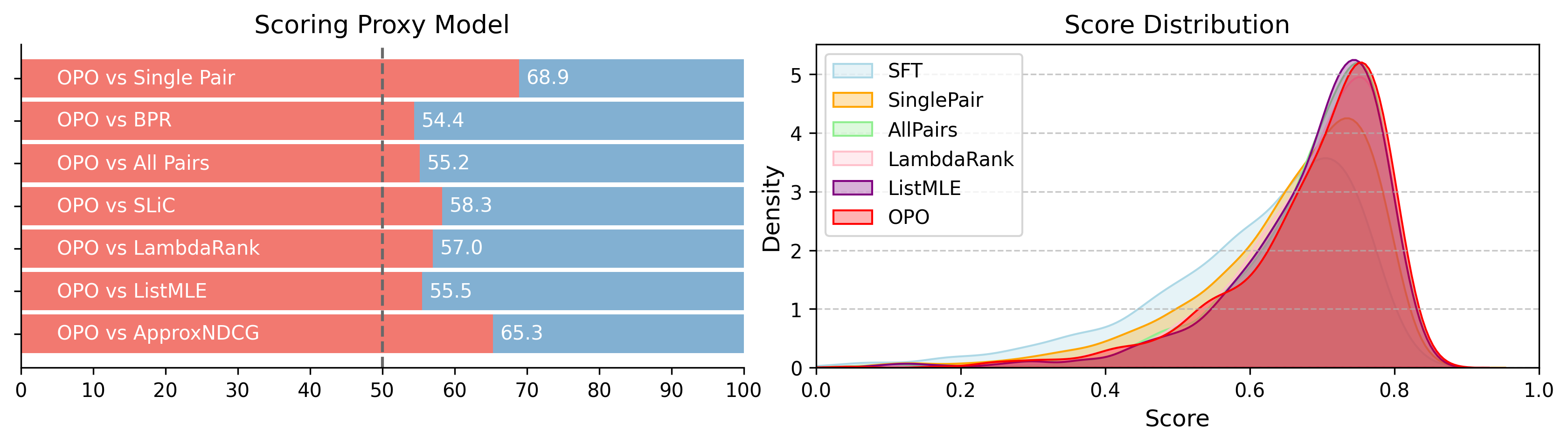
Figure 5: OPO demonstrates superior performance compared to other methods in Scoring Proxy model win rates on Mistral-7B, while also shifting the distribution of response reward scores more significantly to the right (i.e., increasing reward scores).

A.5 ApproxNDCG Analysis

The ApproxNDCG method performs poorly, possibly due to the following reasons: (1) The position function is an approximation, leading to error accumulation. (2) The sigmoid function used for the approximation of the position function may suffer from the vanishing gradient problem [37].

In ApproxNDCG, we observe similar results to NeuralNDCG; the model achieves optimal performance only when the approximation accuracy reaches a certain threshold. First, we prove that the Accuracy of ApproxNDCG is relevant to the multiplication of $\alpha$ and $\beta$ when we employ the score function in Eq 2:

$$\widehat{\tau(j)} =1+\sum_{i\neq j}\frac{\exp{(-\alpha(s_{j}-s_{i}))}}{1+\exp{(-\alpha(s_{j}-s_{i}))}}==1+\sum_{i\neq j}\frac{1}{1+\exp(\alpha(s_{j}-s_{i}))}$$ (19)

$$=1+\sum_{i\neq j}\frac{1}{1+\exp(\alpha\beta)(\log\frac{\pi_{\theta}(y_{j}|x)}{\pi_{ref}(y_{j}|x)}-\log\frac{\pi_{\theta}(y_{i}|x)}{\pi_{ref}(y_{i}|x)})}$$

$$=1+\sum_{i\neq j}\frac{1}{1+\exp(\alpha\beta)\times\frac{\pi_{\theta}(y_{j}|x)\pi_{ref}(y_{i}|x)}{\pi_{ref}(y_{j}|x)\pi_{\theta}(y_{i}|x)}}$$

$$=1+\sum_{i\neq j}\frac{\pi_{ref}(y_{j}|x)\pi_{\theta}(y_{i}|x)}{\pi_{ref}(y_{j}|x)\pi_{\theta}(y_{i}|x)+\exp(\alpha\beta)\times\pi_{\theta}(y_{j}|x)\pi_{ref}(y_{i}|x)}$$

Then, we illustrate the Approximation accuracy and model performance of ApproxNDCG with different hyperparameters $\alpha\cdot\beta$ in Fig 6.

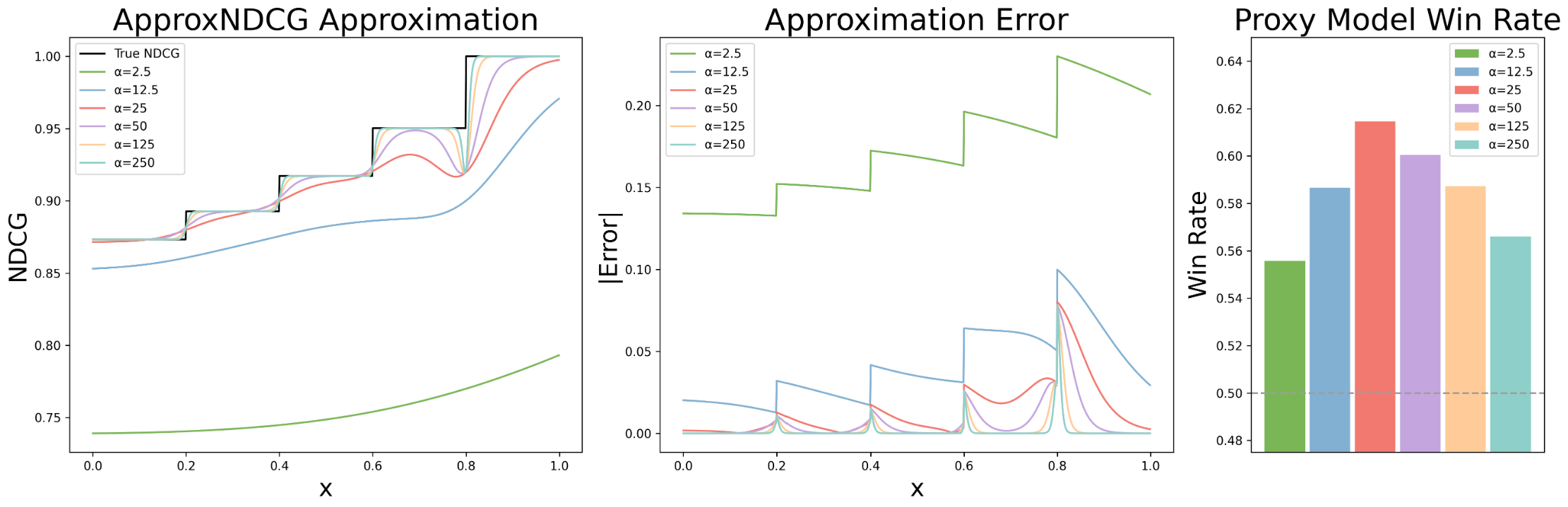
Figure 6: Given ground truth label $\psi=[1.0,0.8,0.6,0.4,0.2]$, the scores $\mathbf{s}=[x,0.8,0.6,0.4,0.2]$ and fix $\beta=0.1$, we visualize the ApproxNDCG Approximation Accuracy with different $\alpha$ and its corresponding absolute value of error and Pair-Preference proxy model win rate against SFT model.

Notice that the approximation accuracy of ApproxNDCG decreases as $\alpha$ increases, which is opposite to NeuralNDCG.

A.6 Training Efficiency

The computational complexity of each method depends on calculating $\pi_{\theta}(y_{j}|x)$ and $\pi_{\text{ref}}(y_{j}|x)$ for each $y_{j}\in\{\mathbf{Y}\}$ to get corresponding scores in Eq 2, which is $\mathcal{O}(K)$, where K is the list size of multiple responses. Subsequently, the pairwise comparison of multiple responses can be efficiently computed using PyTorch’s broadcasting mechanism to perform matrix subtraction.The resulting matrix $P[i,j]$ represents the value of $s_{i}-s_{j}$ . Therefore, for pairwise methods, it suffices to consider only the upper triangular matrix, excluding diagonal elements. This approach does not significantly increase training time when performing pairwise comparisons. The training time and GPU memory usage of Mistral-7B model is shown in Table 11.

Run Name	List Size	Training Time	GPU Memory Usage
Single Pair	2	3h 28m	92.44%
BPR	8	12h 42m	93.43%
All Pairs	8	12h 38m	93.63%
SLiC	8	11h 42m	93.79%
LambdaRank	8	12h 14m	93.66%
ListMLE	8	12h 26m	93.29%
ApproxNDCG	8	12h 56m	93.64%
OPO	8	11h 39m	93.73%

Table 11: Training Time and GPU memory usage on 16$\times$Nvidia V100-32G with Mistral-7B.

It is important to note that specific training times and GPU memory usage can exhibit random fluctuations. This result is intended to demonstrate that the training times for pairwise and listwise methods on multiple responses with the same list size do not show significant differences.

A.7 Response Samples

We select generated response samples on Mistral-7B to further illustrate the enhanced performance of OPO in Table 12 and Table 13.

Method	SFT	Single Pair	BPR	All Pairs	SLiC	LambdaRank	ListMLE	ApproxNDCG	OPO
Length	828	877	1096	1054	1023	1140	1041	1284	1120

Table 12: Average response length on AlpacaEval dataset on Mistral-7B.

Table 13: OPO generates a longer and more detailed response on AlpacaEval in the following samples and outperforms other methods in quality judged by GPT-4 Turbo on Mistral-7B.

Prompt	Q: Who is Larry Page?
SFT	Larry Page is the co-founder and former CEO of Google, a multinational technology company. He is also the co-founder of Alphabet Inc., the parent company of Google. Page is known for his contributions to the development of the PageRank algorithm, which is used to determine the importance of websites in search engine rankings. He is also involved in various philanthropic efforts, including the creation of the Google Foundation, which supports projects related to education, health, and the environment.
OPO	Larry Page is a co-founder, former CEO, and current CEO of Alphabet Inc., the parent company of Google. He was born on March 26, 1973, in East Lansing, Michigan, and graduated from Stanford University with a degree in computer science and artificial intelligence. Page, along with Sergey Brin, developed the PageRank algorithm, which forms the basis of Google’s search engine. In 1998, they founded Google, which quickly became one of the most successful and influential technology companies in the world. Page served as Google’s CEO from 1999 to 2001 and again from 2011 to 2015, during which time he oversaw the company’s expansion into new markets, including mobile devices, cloud computing, and artificial intelligence. In 2015, Page stepped down as CEO of Google and became the CEO of Alphabet, the holding company that was created to separate Google’s core internet business from its other ventures. As Alphabet’s CEO, Page has focused on developing new technologies and expanding into emerging markets, such as healthcare and autonomous vehicles. Page is widely regarded as one of the most innovative and influential entrepreneurs of our time, and his contributions to the field of computer science and technology have had a profound impact on the world.

Single Pair	Larry Page is an American entrepreneur, computer scientist, and co-founder of Google, along with Sergey Brin. He was born on March 26, 1973, in East Lansing, Michigan, and graduated from Stanford University with a degree in computer science and artificial intelligence. Page is known for his innovative ideas and leadership in the technology industry, particularly in the areas of search engines, artificial intelligence, and renewable energy. He currently serves as the CEO of Alphabet Inc., the parent company of Google, and is considered one of the most influential figures in the tech world.
BPR	Larry Page is a co-founder of Google, along with Sergey Brin. He was born on March 26, 1973, in East Lansing, Michigan, USA. Page and Brin started Google in 1998 while they were both PhD students at Stanford University. Page’s primary role in the company has been as CEO from 2001 to 2019, and he currently serves as the CEO of Alphabet Inc., the parent company of Google. Under his leadership, Google has become one of the most successful and influential technology companies in the world, with a market capitalization of over $1 trillion. Page is also known for his philanthropic efforts, including funding research on renewable energy and supporting education initiatives.
All Pairs	Larry Page is a co-founder of Google, along with Sergey Brin. He was born on March 26, 1973, in East Lansing, Michigan, USA. Page and Brin started Google in 1998 while they were both PhD students at Stanford University. Page is known for his focus on innovation, simplicity, and user experience, and he has been instrumental in shaping Google’s vision and strategy. He served as CEO of Alphabet Inc., the parent company of Google, from 2015 to 2019, and currently serves as the CEO of Alphabet’s subsidiary, Google. Page is also a philanthropist and has been involved in various charitable initiatives, including the PageRipples Foundation, which supports education and environmental causes.
SLiC	Larry Page is a co-founder of Google, along with Sergey Brin. He was born on March 26, 1973, in East Lansing, Michigan, USA. Page and Brin started Google in 1998 while they were both PhD students at Stanford University. Page is currently the CEO of Alphabet Inc., the parent company of Google, and is responsible for overseeing the company’s overall strategy and direction. He is also a prominent figure in the technology industry, known for his focus on innovation, sustainability, and philanthropy.

LambdaRank	Larry Page is a co-founder of Google, along with Sergey Brin. He was born on March 26, 1973, in East Lansing, Michigan, USA. Page and Brin started Google in 1998 while they were both PhD students at Stanford University. Page served as the CEO of Google from 1999 to 2001, and then again from 2011 to 2015. He currently serves as the CEO of Alphabet Inc., the parent company of Google. Page is known for his focus on innovation, sustainability, and philanthropy, and has been recognized as one of the most influential people in the world.
ListMLE	Larry Page is a co-founder of Google, along with Sergey Brin. He was born on March 26, 1973, in East Lansing, Michigan, USA. Page and Brin started Google in 1998 while they were both PhD students at Stanford University. Page is currently the CEO of Alphabet Inc., the parent company of Google, and is responsible for overseeing the company’s overall strategy and direction. He is also a prominent figure in the technology industry, known for his focus on innovation, sustainability, and philanthropy.
ApproxNDCG	Larry Page is a co-founder of Google, along with Sergey Brin. He was born on March 26, 1973, in East Lansing, Michigan, and grew up in the Detroit area. Page and Brin met at Stanford University, where they developed the PageRank algorithm, which became the basis for Google’s search engine.\n\n Page served as the CEO of Google from 1999 to 2001, and then again from 2011 to 2019. During his tenure, he oversaw the company’s growth and expansion, including the development of new products and services, such as Google Maps, Google Earth, and Google Glass.\n\n Page is known for his focus on innovation, user experience, and sustainability. He has also been involved in various philanthropic efforts, including the creation of the Google.org foundation and the development of the Google Self-Driving Car Project.\n\n Today, Page is the CEO of Alphabet, the parent company of Google, and continues to play a key role in shaping the future of technology and the internet.

References

- qwe [2024] Qwen2 technical report. 2024.
- Achiam et al. [2023] Josh Achiam, Steven Adler, Sandhini Agarwal, Lama Ahmad, Ilge Akkaya, Florencia Leoni Aleman, Diogo Almeida, Janko Altenschmidt, Sam Altman, Shyamal Anadkat, et al. Gpt-4 technical report. arXiv preprint arXiv:2303.08774, 2023.
- Azar et al. [2024] Mohammad Gheshlaghi Azar, Zhaohan Daniel Guo, Bilal Piot, Remi Munos, Mark Rowland, Michal Valko, and Daniele Calandriello. A general theoretical paradigm to understand learning from human preferences. In International Conference on Artificial Intelligence and Statistics, pages 4447–4455. PMLR, 2024.
- Bai et al. [2022] Yuntao Bai, Andy Jones, Kamal Ndousse, Amanda Askell, Anna Chen, Nova DasSarma, Dawn Drain, Stanislav Fort, Deep Ganguli, Tom Henighan, et al. Training a helpful and harmless assistant with reinforcement learning from human feedback. arXiv preprint arXiv:2204.05862, 2022.
- Bradley and Terry [1952] Ralph Allan Bradley and Milton E Terry. Rank analysis of incomplete block designs: I. the method of paired comparisons. Biometrika, 39(3/4):324–345, 1952.
- Burges et al. [2006] Christopher Burges, Robert Ragno, and Quoc Le. Learning to rank with nonsmooth cost functions. Advances in neural information processing systems, 19, 2006.
- Chen et al. [2020] Ting Chen, Simon Kornblith, Mohammad Norouzi, and Geoffrey Hinton. A simple framework for contrastive learning of visual representations. In International conference on machine learning, pages 1597–1607. PMLR, 2020.
- Christiano et al. [2017] Paul F Christiano, Jan Leike, Tom Brown, Miljan Martic, Shane Legg, and Dario Amodei. Deep reinforcement learning from human preferences. Advances in neural information processing systems, 30, 2017.
- Cui et al. [2023] Ganqu Cui, Lifan Yuan, Ning Ding, Guanming Yao, Wei Zhu, Yuan Ni, Guotong Xie, Zhiyuan Liu, and Maosong Sun. UltraFeedback: Boosting language models with high-quality feedback. arXiv preprint arXiv:2310.01377, 2023.
- Ding et al. [2023] Ning Ding, Yulin Chen, Bokai Xu, Yujia Qin, Zhi Zheng, Shengding Hu, Zhiyuan Liu, Maosong Sun, and Bowen Zhou. Enhancing chat language models by scaling high-quality instructional conversations, 2023.
- Dong et al. [2023] Hanze Dong, Wei Xiong, Deepanshu Goyal, Yihan Zhang, Winnie Chow, Rui Pan, Shizhe Diao, Jipeng Zhang, Kashun Shum, and Tong Zhang. Raft: Reward ranked finetuning for generative foundation model alignment. arXiv preprint arXiv:2304.06767, 2023.
- Dong et al. [2024] Hanze Dong, Wei Xiong, Bo Pang, Haoxiang Wang, Han Zhao, Yingbo Zhou, Nan Jiang, Doyen Sahoo, Caiming Xiong, and Tong Zhang. Rlhf workflow: From reward modeling to online rlhf, 2024.
- Donmez et al. [2009] Pinar Donmez, Krysta M Svore, and Christopher JC Burges. On the local optimality of lambdarank. In Proceedings of the 32nd international ACM SIGIR conference on Research and development in information retrieval, pages 460–467, 2009.
- Dubey et al. [2024] Abhimanyu Dubey, Abhinav Jauhri, Abhinav Pandey, Abhishek Kadian, Ahmad Al-Dahle, Aiesha Letman, Akhil Mathur, Alan Schelten, Amy Yang, Angela Fan, et al. The llama 3 herd of models. arXiv preprint arXiv:2407.21783, 2024.
- Ethayarajh et al. [2024] Kawin Ethayarajh, Winnie Xu, Niklas Muennighoff, Dan Jurafsky, and Douwe Kiela. Kto: Model alignment as prospect theoretic optimization. arXiv preprint arXiv:2402.01306, 2024.
- Grover et al. [2019] Aditya Grover, Eric Wang, Aaron Zweig, and Stefano Ermon. Stochastic optimization of sorting networks via continuous relaxations. arXiv preprint arXiv:1903.08850, 2019.
- Hidasi et al. [2016] Balázs Hidasi, Alexandros Karatzoglou, Linas Baltrunas, and Domonkos Tikk. Session-based recommendations with recurrent neural networks, 2016. URL https://arxiv.org/abs/1511.06939.
- Hong et al. [2024] Jiwoo Hong, Noah Lee, and James Thorne. Orpo: Monolithic preference optimization without reference model, 2024. URL https://arxiv.org/abs/2403.07691.
- Järvelin and Kekäläinen [2002] Kalervo Järvelin and Jaana Kekäläinen. Cumulated gain-based evaluation of ir techniques. ACM Trans. Inf. Syst., 20(4):422–446, oct 2002. ISSN 1046-8188. doi: 10.1145/582415.582418. URL https://doi.org/10.1145/582415.582418.
- Jiang et al. [2023] Albert Q. Jiang, Alexandre Sablayrolles, Arthur Mensch, Chris Bamford, Devendra Singh Chaplot, Diego de las Casas, Florian Bressand, Gianna Lengyel, Guillaume Lample, Lucile Saulnier, Lélio Renard Lavaud, Marie-Anne Lachaux, Pierre Stock, Teven Le Scao, Thibaut Lavril, Thomas Wang, Timothée Lacroix, and William El Sayed. Mistral 7b, 2023. URL https://arxiv.org/abs/2310.06825.
- Karatzoglou et al. [2013] Alexandros Karatzoglou, Linas Baltrunas, and Yue Shi. Learning to rank for recommender systems. In Proceedings of the 7th ACM Conference on Recommender Systems, pages 493–494, 2013.
- Kim et al. [2024] Dahyun Kim, Yungi Kim, Wonho Song, Hyeonwoo Kim, Yunsu Kim, Sanghoon Kim, and Chanjun Park. sdpo: Don’t use your data all at once. arXiv preprint arXiv:2403.19270, 2024.
- Kingma and Ba [2014] Diederik P Kingma and Jimmy Ba. Adam: A method for stochastic optimization. arXiv preprint arXiv:1412.6980, 2014.
- Köpf et al. [2024] Andreas Köpf, Yannic Kilcher, Dimitri von Rütte, Sotiris Anagnostidis, Zhi Rui Tam, Keith Stevens, Abdullah Barhoum, Duc Nguyen, Oliver Stanley, Richárd Nagyfi, et al. Openassistant conversations-democratizing large language model alignment. Advances in Neural Information Processing Systems, 36, 2024.
- Lambert et al. [2024] Nathan Lambert, Valentina Pyatkin, Jacob Morrison, LJ Miranda, Bill Yuchen Lin, Khyathi Chandu, Nouha Dziri, Sachin Kumar, Tom Zick, Yejin Choi, Noah A. Smith, and Hannaneh Hajishirzi. Rewardbench: Evaluating reward models for language modeling, 2024.
- Li et al. [2023] Xuechen Li, Tianyi Zhang, Yann Dubois, Rohan Taori, Ishaan Gulrajani, Carlos Guestrin, Percy Liang, and Tatsunori B. Hashimoto. Alpacaeval: An automatic evaluator of instruction-following models. https://github.com/tatsu-lab/alpaca_eval, 2023.
- Li et al. [2024] Yongqi Li, Nan Yang, Liang Wang, Furu Wei, and Wenjie Li. Learning to rank in generative retrieval. In Proceedings of the AAAI Conference on Artificial Intelligence, volume 38, pages 8716–8723, 2024.
- Liu et al. [2023] Tianqi Liu, Yao Zhao, Rishabh Joshi, Misha Khalman, Mohammad Saleh, Peter J Liu, and Jialu Liu. Statistical rejection sampling improves preference optimization. arXiv preprint arXiv:2309.06657, 2023.
- Liu et al. [2024] Tianqi Liu, Zhen Qin, Junru Wu, Jiaming Shen, Misha Khalman, Rishabh Joshi, Yao Zhao, Mohammad Saleh, Simon Baumgartner, Jialu Liu, Peter J. Liu, and Xuanhui Wang. Lipo: Listwise preference optimization through learning-to-rank, 2024. URL https://arxiv.org/abs/2402.01878.
- Liu et al. [2009] Tie-Yan Liu et al. Learning to rank for information retrieval. Foundations and Trends® in Information Retrieval, 3(3):225–331, 2009.
- Meng et al. [2024] Yu Meng, Mengzhou Xia, and Danqi Chen. SimPO: Simple preference optimization with a reference-free reward. arXiv preprint arXiv:2405.14734, 2024.
- Ouyang et al. [2022] Long Ouyang, Jeffrey Wu, Xu Jiang, Diogo Almeida, Carroll Wainwright, Pamela Mishkin, Chong Zhang, Sandhini Agarwal, Katarina Slama, Alex Ray, et al. Training language models to follow instructions with human feedback. Advances in neural information processing systems, 35:27730–27744, 2022.
- Pang et al. [2024] Richard Yuanzhe Pang, Weizhe Yuan, Kyunghyun Cho, He He, Sainbayar Sukhbaatar, and Jason Weston. Iterative reasoning preference optimization. arXiv preprint arXiv:2404.19733, 2024.
- Park et al. [2024] Ryan Park, Rafael Rafailov, Stefano Ermon, and Chelsea Finn. Disentangling length from quality in direct preference optimization. arXiv preprint arXiv:2403.19159, 2024.
- Plackett [1975] Robin L Plackett. The analysis of permutations. Journal of the Royal Statistical Society Series C: Applied Statistics, 24(2):193–202, 1975.
- Pobrotyn and Białobrzeski [2021] Przemysław Pobrotyn and Radosław Białobrzeski. Neuralndcg: Direct optimisation of a ranking metric via differentiable relaxation of sorting, 2021. URL https://arxiv.org/abs/2102.07831.
- Qin et al. [2010] Tao Qin, Tie-Yan Liu, and Hang Li. A general approximation framework for direct optimization of information retrieval measures. Information retrieval, 13:375–397, 2010.
- Rafailov et al. [2023] Rafael Rafailov, Archit Sharma, Eric Mitchell, Stefano Ermon, Christopher D. Manning, and Chelsea Finn. Direct preference optimization: Your language model is secretly a reward model, 2023. URL https://arxiv.org/abs/2305.18290.
- Rendle et al. [2012] Steffen Rendle, Christoph Freudenthaler, Zeno Gantner, and Lars Schmidt-Thieme. Bpr: Bayesian personalized ranking from implicit feedback, 2012. URL https://arxiv.org/abs/1205.2618.
- Rosset et al. [2024] Corby Rosset, Ching-An Cheng, Arindam Mitra, Michael Santacroce, Ahmed Awadallah, and Tengyang Xie. Direct nash optimization: Teaching language models to self-improve with general preferences. arXiv preprint arXiv:2404.03715, 2024.
- Sinkhorn [1964] Richard Sinkhorn. A relationship between arbitrary positive matrices and doubly stochastic matrices. The annals of mathematical statistics, 35(2):876–879, 1964.
- Song et al. [2024] Feifan Song, Bowen Yu, Minghao Li, Haiyang Yu, Fei Huang, Yongbin Li, and Houfeng Wang. Preference ranking optimization for human alignment, 2024. URL https://arxiv.org/abs/2306.17492.
- Stiennon et al. [2020] Nisan Stiennon, Long Ouyang, Jeffrey Wu, Daniel Ziegler, Ryan Lowe, Chelsea Voss, Alec Radford, Dario Amodei, and Paul F Christiano. Learning to summarize with human feedback. Advances in Neural Information Processing Systems, 33:3008–3021, 2020.
- Team et al. [2023] Gemini Team, Rohan Anil, Sebastian Borgeaud, Yonghui Wu, Jean-Baptiste Alayrac, Jiahui Yu, Radu Soricut, Johan Schalkwyk, Andrew M Dai, Anja Hauth, et al. Gemini: a family of highly capable multimodal models. arXiv preprint arXiv:2312.11805, 2023.
- Tunstall et al. [2023a] Lewis Tunstall, Edward Beeching, Nathan Lambert, Nazneen Rajani, Shengyi Huang, Kashif Rasul, Alexander M. Rush, and Thomas Wolf. The alignment handbook. https://github.com/huggingface/alignment-handbook, 2023a.
- Tunstall et al. [2023b] Lewis Tunstall, Edward Beeching, Nathan Lambert, Nazneen Rajani, Kashif Rasul, Younes Belkada, Shengyi Huang, Leandro von Werra, Clémentine Fourrier, Nathan Habib, Nathan Sarrazin, Omar Sanseviero, Alexander M. Rush, and Thomas Wolf. Zephyr: Direct distillation of lm alignment, 2023b.
- Valizadegan et al. [2009a] Hamed Valizadegan, Rong Jin, Ruofei Zhang, and Jianchang Mao. Learning to rank by optimizing ndcg measure. Advances in neural information processing systems, 22, 2009a.
- Valizadegan et al. [2009b] Hamed Valizadegan, Rong Jin, Ruofei Zhang, and Jianchang Mao. Learning to rank by optimizing ndcg measure. Advances in neural information processing systems, 22, 2009b.
- Vargas and Castells [2011] Saúl Vargas and Pablo Castells. Rank and relevance in novelty and diversity metrics for recommender systems. In Proceedings of the fifth ACM conference on Recommender systems, pages 109–116, 2011.
- Wang et al. [2024] Haoxiang Wang, Wei Xiong, Tengyang Xie, Han Zhao, and Tong Zhang. Interpretable preferences via multi-objective reward modeling and mixture-of-experts. arXiv preprint arXiv:2406.12845, 2024.
- Wang et al. [2020] Yixin Wang, Dawen Liang, Laurent Charlin, and David M. Blei. Causal inference for recommender systems. In Proceedings of the 14th ACM Conference on Recommender Systems, RecSys ’20, page 426–431, New York, NY, USA, 2020. Association for Computing Machinery. ISBN 9781450375832. doi: 10.1145/3383313.3412225. URL https://doi.org/10.1145/3383313.3412225.
- Xia et al. [2008a] Fen Xia, Tie-Yan Liu, Jue Wang, Wensheng Zhang, and Hang Li. Listwise approach to learning to rank: theory and algorithm. In Proceedings of the 25th international conference on Machine learning, pages 1192–1199, 2008a.
- Xia et al. [2008b] Fen Xia, Tie-Yan Liu, Jue Wang, Wensheng Zhang, and Hang Li. Listwise approach to learning to rank: theory and algorithm. In Proceedings of the 25th international conference on Machine learning, pages 1192–1199, 2008b.
- Xu et al. [2023] Jing Xu, Andrew Lee, Sainbayar Sukhbaatar, and Jason Weston. Some things are more cringe than others: Preference optimization with the pairwise cringe loss. arXiv preprint arXiv:2312.16682, 2023.
- Yin et al. [2024] Yueqin Yin, Zhendong Wang, Yi Gu, Hai Huang, Weizhu Chen, and Mingyuan Zhou. Relative preference optimization: Enhancing llm alignment through contrasting responses across identical and diverse prompts. arXiv preprint arXiv:2402.10958, 2024.
- Yuan et al. [2024] Weizhe Yuan, Richard Yuanzhe Pang, Kyunghyun Cho, Sainbayar Sukhbaatar, Jing Xu, and Jason Weston. Self-rewarding language models. arXiv preprint arXiv:2401.10020, 2024.
- Yuan et al. [2023] Zheng Yuan, Hongyi Yuan, Chuanqi Tan, Wei Wang, Songfang Huang, and Fei Huang. Rrhf: Rank responses to align language models with human feedback without tears, 2023. URL https://arxiv.org/abs/2304.05302.
- Zhao et al. [2023] Yao Zhao, Rishabh Joshi, Tianqi Liu, Misha Khalman, Mohammad Saleh, and Peter J. Liu. Slic-hf: Sequence likelihood calibration with human feedback, 2023. URL https://arxiv.org/abs/2305.10425.
- Zheng et al. [2023] Lianmin Zheng, Wei-Lin Chiang, Ying Sheng, Siyuan Zhuang, Zhanghao Wu, Yonghao Zhuang, Zi Lin, Zhuohan Li, Dacheng Li, Eric. P Xing, Hao Zhang, Joseph E. Gonzalez, and Ion Stoica. Judging llm-as-a-judge with mt-bench and chatbot arena, 2023.
- Zhu et al. [2024] Mingye Zhu, Yi Liu, Lei Zhang, Junbo Guo, and Zhendong Mao. Lire: listwise reward enhancement for preference alignment. arXiv preprint arXiv:2405.13516, 2024.
- Ziegler et al. [2019] Daniel M Ziegler, Nisan Stiennon, Jeffrey Wu, Tom B Brown, Alec Radford, Dario Amodei, Paul Christiano, and Geoffrey Irving. Fine-tuning language models from human preferences. arXiv preprint arXiv:1909.08593, 2019.