DeepONet for Solving PDEs: Generalization Analysis in Sobolev Training

Abstract

In this paper, we investigate the application of operator learning, specifically DeepONet, to solve partial differential equations (PDEs). Unlike function learning methods that require training separate neural networks for each PDE, operator learning generalizes across different PDEs without retraining. We focus on the performance of DeepONet in Sobolev training, addressing two key questions: the approximation ability of deep branch and trunk networks, and the generalization error in Sobolev norms. Our findings highlight that deep branch networks offer significant performance benefits, while trunk networks are best kept simple. Moreover, standard sampling methods without adding derivative information in the encoding part are sufficient for minimizing generalization error in Sobolev training, based on generalization analysis. This paper fills a theoretical gap by providing error estimations for a wide range of physics-informed machine learning models and applications.

1 INTRODUCTION

Solving Partial Differential Equations (PDEs) using neural networks has been widely applied in mathematical and engineering fields, especially for high-dimensional domains where classical methods, such as finite elements [3], face challenges. Methods for solving PDEs can be broadly divided into two categories: function learning and operator learning. Function learning methods, such as Physics-Informed Neural Networks (PINNs) [29], the Deep Ritz Method [10], the Deep Galerkin Method [34], and approaches based on random features [5, 36, 9], use neural networks to directly approximate the solutions of PDEs by minimizing specifically designed loss functions. A significant limitation of function learning approaches is the need to train a separate neural network for each PDE, especially if it differs from the one on which the network was originally trained. On the other hand, operator learning methods, such as DeepONet [23] and the Fourier Neural Operator (FNO) [20], focus on learning the operator that maps the PDE parameters to their corresponding solutions. These methods are more general and do not require retraining for different PDEs, provided that the underlying differential operator remains unchanged.

Therefore, applying operator learning to solve PDEs is more effective. In this paper, we will study the performance of operator learning in solving PDEs, with a focus on DeepONet [24]. In the DeepONet structure introduced by [24], the architecture is expressed as follows:

$$\sum_{k=1}^{p}\underbrace{\sum_{i=1}^{q}c_{i}^{k}\sigma\left(\sum_{j=1}^{m}\xi_{ij}^{k}s\left(\bm{x}_{j}\right)+\theta_{i}^{k}\right)}_{\text{branch}}\underbrace{\sigma\left(\bm{w}_{k}\cdot\bm{y}+\zeta_{k}\right)}_{\text{trunk}},$$ (1)

where the branch network processes the input function, and the trunk network processes the coordinates. A key difference between this and shallow neural networks for function approximation is the replacement of the coefficient term with a branch network, which itself resembles a shallow neural network. This facilitates the generalization of the structure into a more flexible form, given by:

$$\mathcal{G}(s;\bm{\theta}):=\sum_{k=1}^{p}\underbrace{\mathcal{B}(\mathcal{D}(s);\bm{\theta}_{1,k})}_{\text{branch}}\underbrace{\mathcal{T}(\bm{y};\bm{\theta}_{2,k})}_{\text{trunk}},$$ (2)

where both $\mathcal{B}$ and $\mathcal{T}$ are fully connected DNNs. This kind of the structure has also been mentioned in [25, 19]. Our approach can easily reduce to the shallow neural network case, recovering the classical DeepONet. In Eq. (2), $\mathcal{D}$ denotes a projection that reduces $s$ to a finite-dimensional vector, allowing for various reduction techniques in differential problems, such as the truncation of Fourier and Taylor series or the finite element method [3]. In the classical DeepONet, this projection is based on the sample points.

Note that both the branch and trunk networks can easily be generalized into deep neural networks. As discussed in [23, 42, 40], deep neural networks have been shown to outperform shallow neural networks in terms of approximation error for function approximation. This raises the following question:

Q1: Do the branch and trunk networks have sufficient approximation ability when they are deep neural networks? If so, are their performance in terms of approximation error better than that of shallow neural networks when they are deep neural networks?

The results in this paper show that the branch network benefits from becoming a deep neural network, whereas the trunk network does not. While a deep trunk network may achieve a super-convergence rate—a better rate than $M^{-\frac{s}{d}}$, where $M$ is the number of parameters, $s$ is the smoothness of the function class, and $d$ is the dimension—there are key challenges. First, in this case, most of the parameters in the trunk network depend on the input function $v$. For each parameter that depends on $v$, a branch network is required to approximate it, complicating the structure of DeepONet compared to Eq. (2). Second, this requires the branch network to approximate discontinuous functionals [45], making the task particularly challenging, as deep neural networks typically establish discontinuous approximators [8]. The branch network, however, does not face these issues and can benefit from a deep structure in terms of approximation error. This observation is consistent with the findings in [25], which show that the trunk network is sensitive and difficult to train. Therefore, the trunk network should be kept simple, using methods such as Proper Orthogonal Decomposition (POD) to assist in learning.

The second question arises from applying operator learning to solve PDEs. In [18], they consider the error analysis of DeepONet in the $L^{2}$-norm. However, for solving PDEs such as

$$\begin{cases}\mathcal{L}u=f&\text{in }\Omega,\\ u=0&\text{on }\partial\Omega,\end{cases}$$ (3)

where $\Omega=[0,1]^{d}$ and $\mathcal{L}$ is a second-order differential operator, the loss function should incorporate information about derivatives, similar to the Physics-Informed Neural Network (PINN) loss [29]. Although some papers have applied PINN losses to DeepONet, such as [37, 21, 13], a theoretical gap remains in understanding the generalization error of DeepONet when measured in Sobolev norms.

Q2: What is the generalization error of DeepONet in Sobolev training, and what insights can be drawn to improve the design of DeepONet?

In this paper, we address this question and fill the gap by providing error estimations for a wide range of physics-informed machine learning models and applications. We find that to minimize the error of DeepONet in Sobolev training, the standard sampling methods used in classical DeepONet are still sufficient. This result differs slightly from our initial expectation that, when studying operators in Sobolev spaces, adding derivative information from the input space would be necessary for training. We show that the encoding in operator learning works effectively without incorporating derivative information from the input space. This insight suggests that even in Sobolev training for operator learning, there is no need to overly complicate the network, particularly the encoding part.

1.1 Contributions and Organization of the Paper

The rest of the paper is organized as follows. In Section 2, we introduce the notations used throughout the paper and set up the operator and loss functions from the problem statement. In Section 3, we estimate the approximation rate. In the first subsection, we reduce operator learning to function learning, showing that the trunk network does not benefit from a deep structure. In the second subsection, we reduce functional approximation to function approximation and demonstrate that the encoding of the input space for the operator can still rely on traditional sampling methods, without the need to incorporate derivative information, even in Sobolev training. In the last subsection, we approximate the function and show that the branch network can benefit from a deep structure. In Section 4, we provide the generalization error analysis of DeepONet in Sobolev training. All omitted proofs from the main text are presented in the appendix.

1.2 Related works

Function Learning: Unlike operator learning, function learning focuses on learning a map from a finite-dimensional space to a finite-dimensional space. Many papers have studied the theory of function approximation in Sobolev spaces, such as [27, 30, 31, 32, 33, 42, 40, 39, 28, 44, 45], among others. In [27, 39, 45], the approximation is considered under the assumption of continuous approximators, as mentioned in [8]. However, for deep neural networks, the approximator is often discontinuous, as discussed in [45], which still achieves the optimal approximation rate with respect to the number of parameters. This is one of the benefits of deep structures, and whether this deep structure provides a significant advantage in approximation is a key point of discussion in this work.

Functional Learning: Functional learning can be viewed as a special case of operator learning, where the objective is to map a function to a constant. Several papers have provided theoretical analyses of using neural networks to approximate functionals. In [6], the universal approximation of neural networks for approximating continuous functionals is established. In [35], the authors provide the approximation rate for functionals, while in [41], they address the approximation of functionals without the curse of dimensionality using Barron space methods. In [43], the approximation rate for functionals on spheres is analyzed.

Operator Learning: The operator learning aspect is closely related to this work. In [18, 7], they perform an error analysis of DeepONet; however, their analysis is primarily focused on solving PDEs in the $L^{2}$-norm, and they do not consider network design, i.e., which parts of the network should be deeper and which should be shallow. In [17], the focus is on addressing the curse of dimensionality and providing lower bounds on the number of parameters required to achieve the target rate. In their results, there is a parameter $\gamma$ that obscures the structural information of the network, so the benefit of network architecture in operator learning remains unclear. In [22], they summarize the general theory of operator learning, but the existence of the benefits of deep neural networks is still not explicitly visible in their results. Other works, such as those focusing on Fourier Neural Operators (FNO) [16], explore different types of operators, which differ from the focus of this paper.

2 PRELIMINARIES

2.1 Notations

Let us summarize all basic notations used in the paper as follows:

1. Matrices are denoted by bold uppercase letters. For example, $\bm{A}\in\mathbb{R}^{m\times n}$ is a real matrix of size $m\times n$ and $\bm{A}^{\intercal}$ denotes the transpose of $\bm{A}$.

2. For a $d$-dimensional multi-index $\bm{\alpha}=[\alpha_{1},\alpha_{2},\cdots\alpha_{d}]\in\mathbb{N}^{d}$, we denote several related notations as follows: $(a)~{}|\bm{\alpha}|=\left|\alpha_{1}\right|+\left|\alpha_{2}\right|+\cdots+\left|\alpha_{d}\right|$; $(b)~{}\bm{x}^{\alpha}=x_{1}^{\alpha_{1}}x_{2}^{\alpha_{2}}\cdots x_{d}^{\alpha_{d}},~{}\bm{x}=\left[x_{1},x_{2},\cdots,x_{d}\right]^{\intercal}$; $(c)~{}\bm{\alpha}!=\alpha_{1}!\alpha_{2}!\cdots\alpha_{d}!.$

3. Let $B_{r,|\cdot|}(\bm{x})\subset\mathbb{R}^{d}$ be the closed ball with a center $\bm{x}\in\mathbb{R}^{d}$ and a radius $r$ measured by the Euclidean distance. Similarly, $B_{r,\|\cdot\|_{\ell_{\infty}}}(\bm{x})\subset\mathbb{R}^{d}$ be the closed ball with a center $\bm{x}\in\mathbb{R}^{d}$ and a radius $r$ measured by the $\ell_{\infty}$-norm.

4. Assume $\bm{n}\in\mathbb{N}_{+}^{n}$, then $f(\bm{n})=\bm{O}(g(\bm{n}))$ means that there exists positive $C$ independent of $\bm{n},f,g$ such that $f(\bm{n})\leq Cg(\bm{n})$ when all entries of $\bm{n}$ go to $+\infty$.

5. Define $\sigma_{1}(x):=\sigma(x)=\max\{0,x\}$ and $\sigma_{2}:=\sigma^{2}(x)$. We call the neural networks with activation function $\sigma_{t}$ with $t\leq i$ as $\sigma_{i}$ neural networks ($\sigma_{i}$-NNs). With the abuse of notations, we define $\sigma_{i}:\mathbb{R}^{d}\to\mathbb{R}^{d}$ as $\sigma_{i}(\bm{x})=\left[\begin{array}[]{c}\sigma_{i}(x_{1})\\ \vdots\\ \sigma_{i}(x_{d})\end{array}\right]$ for any $\bm{x}=\left[x_{1},\cdots,x_{d}\right]^{T}\in\mathbb{R}^{d}$.

6. Define $L,W\in\mathbb{N}_{+}$, $W_{0}=d$ and $W_{L+1}=1$, $W_{i}\in\mathbb{N}_{+}$ for $i=1,2,\ldots,L$, then a $\sigma_{i}$-NN $\phi$ with the width $W$ and depth $L$ can be described as follows:

$$\bm{x}=\tilde{\bm{h}}_{0}\stackrel{{\scriptstyle W_{1},b_{1}}}{{\longrightarrow}}\bm{h}_{1}\stackrel{{\scriptstyle\sigma_{i}}}{{\longrightarrow}}\tilde{\bm{h}}_{1}\ldots\tilde{\bm{h}}_{L}\stackrel{{\scriptstyle W_{L+1},b_{L+1}}}{{\longrightarrow}}\phi(\bm{x})=\bm{h}_{L+1},$$

where $\bm{W}_{i}\in\mathbb{R}^{W_{i}\times W_{i-1}}$ and $\bm{b}_{i}\in\mathbb{R}^{W_{i}}$ are the weight matrix and the bias vector in the $i$-th linear transform in $\phi$, respectively, i.e., $\bm{h}_{i}:=\bm{W}_{i}\tilde{\bm{h}}_{i-1}+\bm{b}_{i},~{}\text{ for }i=1,\ldots,L+1$ and $\tilde{\bm{h}}_{i}=\sigma_{i}\left(\bm{h}_{i}\right),\text{ for }i=1,\ldots,L.$ In this paper, an DNN with the width $W$ and depth $L$, means (a) The maximum width of this DNN for all hidden layers less than or equal to $W$. (b) The number of hidden layers of this DNN less than or equal to $L$.

7. Denote $\Omega$ as $[0,1]^{d}$, $D$ as the weak derivative of a single variable function and $D^{\bm{\alpha}}=D^{\alpha_{1}}_{1}D^{\alpha_{2}}_{2}\ldots D^{\alpha_{d}}_{d}$ as the partial derivative where $\bm{\alpha}=[\alpha_{1},\alpha_{2},\ldots,\alpha_{d}]^{T}$ and $D_{i}$ is the derivative in the $i$-th variable. Let $n\in\mathbb{N}$ and $1\leq p\leq\infty$. Then we define Sobolev spaces

$$W^{n,p}(\Omega):=\left\{f\in L^{p}(\Omega):D^{\bm{\alpha}}f\in L^{p}(\Omega)\text{ with }|\bm{\alpha}|\leq n\right\}$$

with a norm

$$\|f\|_{W^{n,p}(\Omega)}:=\left(\sum_{0\leq|\alpha|\leq n}\left\|D^{\bm{\alpha}}f\right\|_{L^{p}(\Omega)}^{p}\right)^{1/p},~{}p<\infty,$$

and $\|f\|_{W^{n,\infty}(\Omega)}:=\max_{0\leq|\alpha|\leq n}\left\|D^{\bm{\alpha}}f\right\|_{L^{\infty}(\Omega)}$. For simplicity, $\|f\|_{W^{n,2}(\Omega)}=\|f\|_{H^{n}(\Omega)}$. Furthermore, for $\bm{f}=(f_{1},f_{2},\ldots,f_{d})$, $\bm{f}\in W^{1,\infty}(\Omega,\mathbb{R}^{d})$ if and only if $f_{i}\in W^{1,\infty}(\Omega)$ for each $i=1,2,\ldots,d$ and $\|\bm{f}\|_{W^{1,\infty}(\Omega,\mathbb{R}^{d})}:=\max_{i=1,\ldots,d}\{\|f_{i}\|_{W^{1,\infty}(\Omega)}\}$.

2.2 Error component in Sobolev training

In this paper, we consider applying DeepONet to solve partial differential equations (PDEs). Without loss of generality, we focus on the following PDEs (3), though our results can be easily generalized to more complex cases. In this paper, we assume that $\mathcal{L}$ satisfies the following conditions:

Assumption 1.

For any $f_{1},f_{2}\in\mathcal{X}\subset W^{n,\infty}(\Omega)$ and $u_{1},u_{2}\in\mathcal{Y}\subset W^{n,\infty}(\Omega)$ for $n\geq 2$, which is the solution of Eq. (3) with source term $f_{1},f_{2}$, the following conditions hold:

(i) There exists a constant $C$ such that

$$\|u_{1}-u_{2}\|_{H^{2}(\Omega)}\leq C\|f_{1}-f_{2}\|_{L^{2}(\Omega)}.$$

(ii) There exists a constant $L$ such that

$$\|u_{1}-u_{2}\|_{W^{n,\infty}(\Omega)}\leq L\|f_{1}-f_{2}\|_{W^{n,\infty}(\Omega)}.$$

The above assumption holds in many cases. For example, based on [12], when $\mathcal{L}$ is a linear elliptic operator with smooth coefficients and $\Omega$ is a polygon (which is valid for $[0,1]^{d}$), condition (i) in Assumption 1 is satisfied. Regarding condition (ii) in Assumption 1, this assumption reflects that the operator we aim to learn is Lipschitz in $W^{n}(\Omega)$, which is a regularity assumption. If the domain is smooth and $\mathcal{L}$ is linear and has smooth coefficients, then $\|u\|_{W^{n+2,\infty}(\Omega)}\leq L\|f\|_{W^{n,\infty}(\Omega)}$ [11], which is a stronger condition than the one we assume here.

Based on above assumption, the equation above has a unique solution, establishing a mapping between the source term $f\in\mathcal{X}$ and the solution $u\in\mathcal{Y}$, denoted as $\mathcal{G}_{*}$. In [24], training such an operator is treated as a black-box approach, i.e., a data-driven method. However, in many cases, there is insufficient data for training, or there may be no data at all. Thus, it becomes crucial to incorporate information from the PDEs into the training process, as demonstrated in [37, 21, 13]. This technique is referred to as Sobolev training.

In other words, we aim to use $\mathcal{G}(~{}\cdot~{};\bm{\theta})$ (see Eq. (2)) to approximate the mapping between $f$ and $u$. The chosen loss function is:

$$L_{D}(\bm{\theta}) :=L_{\text{in}}(\bm{\theta})+\lambda L_{\text{bound}}(\bm{\theta}),$$

$$L_{\text{in}}(\bm{\theta}) :=\int_{\Omega}\int_{\mathcal{X}}|\mathcal{L}\mathcal{G}(f;\bm{\theta})(\bm{y})-f(\bm{y})|^{2}\,\mathrm{d}\bm{y}\,\mathrm{d}\mu_{\mathcal{X}},$$

$$L_{\text{bound}}(\bm{\theta}) :=\int_{\mathcal{X}}\int_{\partial\Omega}|\mathcal{G}(f;\bm{\theta})(\bm{y})|^{2}\,\mathrm{d}\bm{y}\,\mathrm{d}\mu_{\mathcal{X}},$$ (4)

where $\mu_{\mathcal{X}}$ is a measure on $\mathcal{X}$, and $\mathcal{X}$ is the domain of the operator, i.e., $f\in\mathcal{X}$. The constant $\lambda$ balances the boundary and interior terms. The error analysis of $L_{\text{bound}}(\bm{\theta})$ is the classical $L^{2}$ estimation. Since we focus on the Sobolev training part in this paper, we set $\lambda=0$ for simplicity. Due to (i) in Assumption 1, we obtain:

$$L_{D}(\bm{\theta})\leq C\int_{\mathcal{X}}\|\mathcal{G}(f;\bm{\theta})(\bm{y})-\mathcal{G}_{*}(f)(\bm{y})\|^{2}_{H^{2}(\Omega)}\,\mathrm{d}\mu_{\mathcal{X}}.$$ (5)

Furthermore, if we consider that $\mu_{\mathcal{X}}$ is a finite measure on $\mathcal{X}$ and, for simplicity, assume $\int_{\mathcal{X}}\mathrm{d}\mu_{\mathcal{X}}=1$, we have:

$$L_{D}(\bm{\theta})\leq C\sup_{f\in\mathcal{X}}\|\mathcal{G}(f;\bm{\theta})(\bm{y})-\mathcal{G}_{*}(f)(\bm{y})\|^{2}_{H^{2}(\Omega)}.$$ (6)

This error is called the approximation error. The other part of the error comes from the sample, which we refer to as the generalization error. To define this error, we first introduce the following loss, which is the discrete version of $L_{D}(\bm{\theta})$ for $\lambda=0$:

$$L_{S}(\bm{\theta}):=\frac{1}{MP}\sum_{i=1}^{M}\sum_{j=1}^{P}|\mathcal{L}\mathcal{G}(f_{i};\bm{\theta})(\bm{y}_{j})-f_{i}(\bm{y}_{j})|^{2},$$ (7)

where $\bm{y}_{j}$ is an i.i.d. uniform sample in $\Omega$, and $f_{i}$ is an i.i.d. sample based on $\mu_{\mathcal{X}}$.

Then, the generalization error is given by:

$$\mathbb{E}L_{D}(\bm{\theta}_{S})\leq L_{D}(\bm{\theta}_{D})+\mathbb{E}\left[L_{D}(\bm{\theta}_{S})-L_{S}(\bm{\theta}_{S})\right],$$ (8)

where $\bm{\theta}_{D}=\arg\min L_{D}(\bm{\theta})$ and $\bm{\theta}_{S}=\arg\min L_{S}(\bm{\theta})$. The expectation symbol is due to the randomness in sampling $\bm{y}$ and $f$. The generalization error is represented by the last term in Eq. (22).

3 APPROXIMATION ERROR

In this section, we estimate the approximation error, i.e., we aim to establish the appropriate DeepONet structure and bound $\inf_{\bm{\theta}}L_{D}(\bm{\theta})$. The proof sketch is divided into three steps: the first step reduces the operator learning problem to a functional learning problem, the second step reduces functional learning to function learning, and the final step approximates the function. The diagram outlining the proof is shown in Fig. (1).

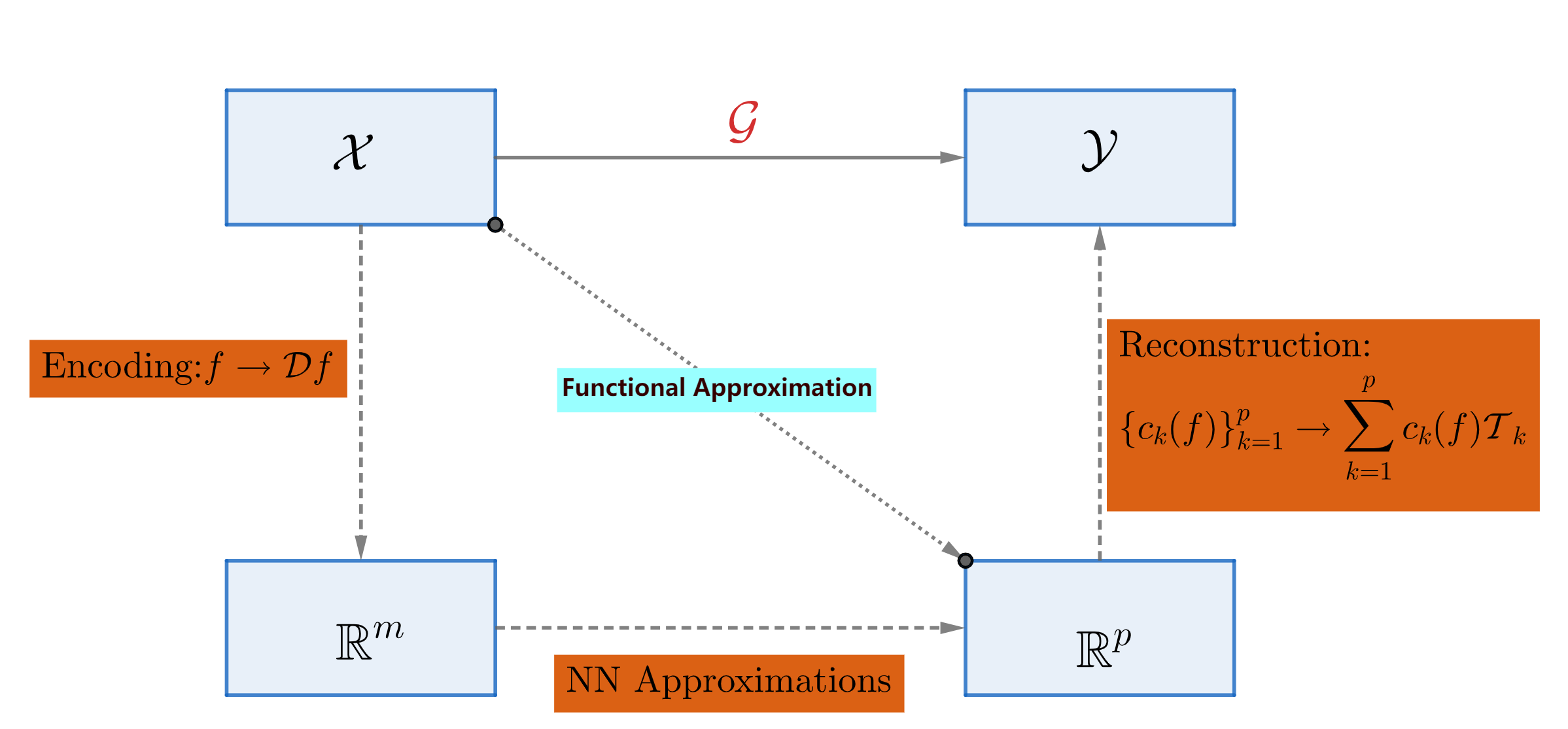
Figure 1: Sketch of the proof for the approximation error.

Theorem 1.

For any $p,m\in\mathbb{N}^{+}$ and sufficiently large $q$, $\lambda\in[1,2]$, and $\mathcal{G}_{*}:\mathcal{X}\subset H^{s}(\mathbb{T}^{d})\to H^{s}(\mathbb{T}^{d})$ with $s>n+\frac{d}{2}$, where $\max\{\|f\|_{W^{n,\infty}(\Omega)},\|f\|_{H^{s}(\Omega)}\}\leq M$ for any $f\in\mathcal{X}$ and $M>0$, satisfying Assumption 1, there exist $\sigma_{2}$-NNs $\mathcal{T}(\bm{y};\bm{\theta}_{2,k})$ with depth $3+\log_{2}d-1+\log_{2}n-1$, width $4n-4+6d$, and a map $\mathcal{D}$ from $\mathcal{X}\to[-M,M]^{m}$, as well as $\sigma_{1}$-NNs $\mathcal{B}(\mathcal{D}f;\bm{\theta}_{k})$ with $C_{1}9^{m}q$ parameters such that:

$$\sup_{f\in\mathcal{X}}\left\|\mathcal{G}_{*}(f)-\sum_{k=1}^{p}\mathcal{B}(\mathcal{D}f;\bm{\theta}_{k})\mathcal{T}(\bm{y};\bm{\theta}_{2,k})\right\|_{H^{2}(\Omega)}\leq C\left(p^{-\frac{n-2}{d}}+p^{\frac{2}{d}}m^{-\frac{s-s^{\prime}}{d}}+m^{\frac{s^{\prime}}{d}}p^{\frac{2}{d}}q^{-\frac{\lambda}{m}}\right),$$ (9)

where $s^{\prime}\in\left(n+\frac{d}{2},s\right)$, and $C,C_{1}$ are independent of $m,p$ and $q$. Furthermore, for $\lambda=1$, $\mathcal{B}(\bm{z};\bm{\theta}_{k})$ is a shallow neural network that can achieve this approximation rate. As $\lambda$ approaches 2, the ratio between the width and depth of $\mathcal{B}$ decreases, implying that the network structure becomes deeper.

Remark 1.

The term $\lambda$ incorporates the benefit of the deep structure of the neural network. This deep structure arises from the branch network rather than the trunk network. In the approximation analysis, the deep structure of the trunk network does not yield benefits; instead, it makes the branch network more difficult to train. We will provide more details on this in the following subsections.

3.1 Operator learning to functional learning in Sobolev spaces

Proposition 1.

For any $p\in\mathbb{N}$ and $v\in\mathcal{Y}\subset W^{n,\infty}(\Omega)$, there exist $p$ $\sigma_{2}$-NNs $\{\mathcal{T}(\bm{y};\bm{\theta}_{2,k})\}_{k=1}^{p}$ and bounded linear functionals $c_{k}:W^{n-1,\infty}(\Omega)\to\mathbb{R}$ such that

$$\left\|v-\sum_{k=1}^{p}c_{k}(v)\mathcal{T}(\bm{y};\bm{\theta}_{2,k})\right\|_{H^{2}(\Omega)}\leq Cp^{-\frac{n-2}{d}}\|v\|_{H^{n}(\Omega)},$$ (10)

where $\mathcal{T}(\bm{y};\bm{\theta}_{2,k})$ is a $\sigma_{2}$-NN with depth $3+\log_{2}d-1+\log_{2}n-1$ and width $4n-4+6d$, and $C$ is a constant independent of $p$ and $v$.

Remark 2.

Before we present the sketch of the proof for Proposition 1, there are some remarks we would like to mention. First, the number of parameters in each $\mathcal{T}(\bm{y};\bm{\theta}_{2,k})$ is independent of $p$ and $f$. This is a generalization of the trunk network in DeepONet. It can easily reduce to the classical DeepONet case by applying a shallow neural network to approximate the trunk, a well-known result that we omit here.

Second, the target function $v$ can be considered in $W^{n,p}(\Omega)$ for a more general case. The method of proof remains the same; the only difference is that we need to assume that for any open set $\Omega_{*}\subset\Omega$, the following inequality holds:

$$\|v\|_{W^{n,p}(\Omega_{*})}|\Omega_{*}|^{-\frac{1}{p}}\leq C\|v\|_{W^{n,p}(\Omega)},$$

for any $v\in\mathcal{Y}$. It is straightforward to verify that this condition holds for $p=\infty$.

The sketch of the proof of Proposition 1 is as follows. First, we divide $\Omega$ into $p$ parts and apply the Bramble–Hilbert Lemma [3, Lemma 4.3.8] to locally approximate $v$ on each part using polynomials. The coefficients of these polynomials can be regarded as continuous linear functionals in $W^{n,\infty}(\Omega)$. Next, we use a partition of unity to combine the local polynomial approximations. Finally, we represent both the polynomials and the partition of unity using neural networks.

Based on Proposition 1, we can reduce the operator learning problem to functional learning as follows:

$$\left\|\mathcal{G}_{*}(f)-\sum_{k=1}^{p}c_{k}(\mathcal{G}_{*}(f))\mathcal{T}(\bm{y};\bm{\theta}_{2,k})\right\|_{H^{2}(\Omega)}\leq Cp^{-\frac{n-2}{d}}\|\mathcal{G}_{*}(f)\|_{H^{n}(\Omega)}\leq Cp^{-\frac{n-2}{d}}\|\mathcal{G}_{*}(f)\|_{W^{n,\infty}(\Omega)}$$

$$\leq Cp^{-\frac{n-2}{d}}\|f\|_{W^{n,\infty}(\Omega)},$$ (11)

where the last inequality follows from Assumption 1. Therefore, without considering the approximation of $c_{k}(\mathcal{G}_{*}(f))$, the approximation error can be bounded by $\sup_{f\in\mathcal{X}}Cp^{-\frac{n-2}{d}}\|f\|_{W^{n,\infty}(\Omega)}$. The next step is to consider the approximation of the functional $c_{k}(\mathcal{G}_{*}(f))$.

The approximation order achieved in Proposition 1 corresponds to the optimal approximation rate for neural networks in the continuous approximation case. If we consider deep neural networks, we can achieve an approximation rate of $p^{-\frac{2(n-2)}{d}}$ using the neural network $\mathcal{T}(\bm{y};\bm{\theta}_{2}(v))$. As discussed in [40], most of the parameters depend on $v$, leading to significant interaction between the trunk and branch networks, which makes the learning process more challenging. Furthermore, this approximator can be a discontinuous one, as highlighted in [45, 39], where the functionals $c_{k}$ may no longer be continuous, thereby invalidating subsequent proofs. Therefore, while it is possible to construct deep neural networks for trunk networks, we do not gain the benefits associated with deep networks, and the approximation process becomes more difficult to learn.

3.2 Functional learning to function learning in Sobolev spaces

In this part, we reduce each functional $c_{k}(\mathcal{G}_{*}(f))$ to a function learning problem by applying a suitable projection $\mathcal{D}$ in Eq. (2) to map $u$ into a finite-dimensional space. To ensure that the error in this step remains small, we require $f-\mathcal{P}\circ\mathcal{D}f$ to be small for a continuous reconstruction operator $\mathcal{P}$, which will be defined later, as shown below:

$$|c_{k}(\mathcal{G}_{*}(f))-c_{k}(\mathcal{G}_{*}(\mathcal{P}\circ\mathcal{D}f))|\leq C\|\mathcal{G}_{*}(f)-\mathcal{G}_{*}(\mathcal{P}\circ\mathcal{D}f)\|_{W^{n,\infty}(\Omega)}$$

$$\leq C\|f-\mathcal{P}\circ\mathcal{D}f\|_{W^{n,\infty}(\Omega)}.$$ (12)

The first inequality holds because $c_{k}$ is a bounded linear functional in $W^{n-1,\infty}(\Omega)$, and thus also a bounded linear functional in $W^{n,\infty}(\Omega)$. The second inequality follows from (ii) in Assumption 1.

For the traditional DeepONet [24], $\mathcal{D}$ is a sampling method, i.e.,

$$\mathcal{D}(f)=(f(\bm{x}_{1}),f(\bm{x}_{2}),\cdots,f(\bm{x}_{m})),$$

and then a proper basis is found such that $\mathcal{P}\circ\mathcal{D}(f)=\sum_{j=1}^{m}\alpha_{j}(\mathcal{D}(f))\phi_{j}(\bm{x})$. To achieve this reduction in $W^{n,\infty}(\Omega)$, one approach is to apply pseudo-spectral projection, as demonstrated in [26, 4] and used in the approximation analysis of Fourier Neural Operators (FNO) in [16].

Proposition 2.

For any $f\in H^{s}(\mathbb{T}^{d})$ with $s>n+\frac{d}{2}$, where $H^{s}(\mathbb{T}^{d})$ denotes the functions in $H^{s}(\Omega)$ with periodic boundary conditions, define

$$\mathcal{D}(f)=(f(\bm{x}_{\bm{\nu}}))_{\bm{\nu}\in\{0,1,\ldots,2N\}^{d}}$$

for $\bm{x}_{\bm{\nu}}=\frac{\bm{\nu}}{2N+1}$. Thus, there exists a Lipschitz continuous map $\mathcal{P}:[-M,M]^{m}\to H^{s^{\prime}}(\mathbb{T}^{d})$ such that

$$\|f-\mathcal{P}\circ\mathcal{D}(f)\|_{W^{n,\infty}(\Omega)}\leq CN^{s^{\prime}-s}\|f\|_{H^{s}(\Omega)},$$ (13)

for any $s^{\prime}\in\left(n+\frac{d}{2},s\right)$, where $M=\|f\|_{L^{\infty}(\Omega)}$, $C$ is independent of $N$ and $f$, and $m=(2N+1)^{d}$. Furthermore, the Lipschitz constant of $\mathcal{P}$ is $\bm{O}(N^{s^{\prime}})$.

Remark 3.

In [18, 16], it is shown that the decay rate of the decoder can be exponential if the coefficients of the expansion of the input function decay exponentially, as in the case of holomorphic functions, which contain a very low-dimensional structure [28].

Based on Proposition 2, we can reduce functional learning to function learning. Note that, even though we are considering Sobolev training for operator learning, we do not need derivative information in the encoding process. Specifically, the projection $\mathcal{D}$ defined as $\mathcal{D}(f)=(f(\bm{x}_{\bm{\nu}}))_{\bm{\nu}\in\{0,1,\ldots,2N\}^{d}}$ is sufficient for tasks like solving PDEs. Therefore, when designing operator neural networks for solving PDEs, it is not necessary to include derivative information of the input space in the domain. However, whether adding derivative information in the encoding helps improve the effectiveness of Sobolev training remains an open question, which we will address in future work.

3.3 Function learning in Sobolev spaces

In this part, we will use a neural network to approximate each functional $c_{k}(\mathcal{G}_{*}\circ\mathcal{P}\circ\mathcal{D}(f))$, i.e., we aim to make

$$\sup_{f\in\mathcal{X}}\left|c_{k}(\mathcal{G}_{*}\circ\mathcal{P}\circ\mathcal{D}(f))-\mathcal{B}(\mathcal{D}(f);\bm{\theta}_{1,k})\right|$$ (14)

as small as possible. For simplicity, we consider all functions in $\mathcal{X}$ with $\|f\|_{L^{\infty}(\Omega)}\leq M$ for some $M>0$. We then need to construct a neural network in $[-M,M]^{m}$ such that

$$\sup_{\bm{z}\in[-M,M]^{m}}\left|c_{k}(\mathcal{G}_{*}\circ\mathcal{P}(\bm{z}))-\mathcal{B}(\bm{z};\bm{\theta}_{1,k})\right|$$ (15)

is small. The idea for achieving this approximation is to first analyze the regularity of $c_{k}(\mathcal{G}_{*}\circ\mathcal{P}(\bm{z}))$ with respect to $\bm{z}$. Once the regularity is established, we can construct a neural network that approximates it with a rate that depends on the regularity.

Lemma 1.

Suppose $\mathcal{G}_{*}$ is an operator satisfying Assumption 1 with domain $\mathcal{X}\subset H^{s^{\prime}}(\mathbb{T}^{d})$, where $s^{\prime}>n+\frac{d}{2}$, and $\sup_{f\in\mathcal{X}}\|f\|_{L^{\infty}(\Omega)}\leq M$ for some $M>0$. Let $c_{k}$ be the functional defined in Proposition 1, and $\mathcal{P}$ be the map defined in Proposition 2. Then, $c_{k}(\mathcal{G}_{*}\circ\mathcal{P}(\bm{z}))\in W^{1,\infty}([-M,M]^{m})$, with its norm being $\bm{O}(m^{\frac{s^{\prime}}{d}})$.

Proof.

For any $\bm{z}_{1},\bm{z}_{2}\in[-M,M]^{m}$, we have

$$|c_{k}(\mathcal{G}_{*}\circ\mathcal{P}(\bm{z}_{1}))-c_{k}(\mathcal{G}_{*}\circ\mathcal{P}(\bm{z}_{2}))|$$

$$\leq C\|\mathcal{G}_{*}\circ\mathcal{P}(\bm{z}_{1})-\mathcal{G}_{*}\circ\mathcal{P}(\bm{z}_{2})\|_{W^{n,\infty}(\Omega)},$$ (16)

which holds because $c_{k}$ is a bounded linear functional in $W^{n-1,\infty}(\Omega)$, and thus also a bounded linear functional in $W^{n,\infty}(\Omega)$.

Next, based on the Lipschitz condition of $\mathcal{G}_{*}$ in Assumption 1, we have

$$C\|\mathcal{G}_{*}\circ\mathcal{P}(\bm{z}_{1})-\mathcal{G}_{*}\circ\mathcal{P}(\bm{z}_{2})\|_{W^{n,\infty}(\Omega)}$$

$$\leq C\|\mathcal{P}(\bm{z}_{1})-\mathcal{P}(\bm{z}_{2})\|_{W^{n,\infty}(\Omega)}\leq C\|\mathcal{P}(\bm{z}_{1})-\mathcal{P}(\bm{z}_{2})\|_{H^{s^{\prime}}(\Omega)},$$ (17)

where the last inequality is due to the Sobolev embedding theorem and $s^{\prime}>n+\frac{d}{2}$.

Finally, based on the Lipschitz condition of $\mathcal{P}$ proved in Proposition 2, we have

$$C\|\mathcal{P}(\bm{z}_{1})-\mathcal{P}(\bm{z}_{2})\|_{H^{s^{\prime}}(\Omega)}\leq Cm^{\frac{s^{\prime}}{d}}|\bm{z}_{1}-\bm{z}_{2}|.$$ (18)

Therefore, $c_{k}(\mathcal{G}_{*}\circ\mathcal{P}(\bm{z}))$ is Lipschitz continuous in $[-M,M]^{m}$. Since $[-M,M]^{m}$ is a convex set, by [14], we conclude that $c_{k}(\mathcal{G}_{*}\circ\mathcal{P}(\bm{z}))\in W^{1,\infty}([-M,M]^{m})$, with its norm being $\bm{O}(m^{\frac{s^{\prime}}{d}})$. ∎

Now, we can establish a neural network to approximate $c_{k}(\mathcal{G}_{*}\circ\mathcal{P}(\bm{z}))$. For shallow neural networks, the result from [27] is as follows:

Lemma 2 ([27]).

Suppose $\sigma$ is a continuous non-polynomial function, and $\mathbb{K}$ is a compact subset of $\mathbb{R}^{m}$. Then, there exist positive integers $W$, and constants $w_{k},\zeta_{k},c_{k}$ for $k=1,\ldots,W$, such that for any $v\in W^{1,\infty}(\mathbb{K})$,

$$\left\|v-\sum_{k=1}^{W}c_{k}\sigma\left(\bm{w}_{k}\cdot\bm{z}+\zeta_{k}\right)\right\|_{L^{\infty}(\mathbb{K})}\leq CW^{-1/m}\|v\|_{W^{1,\infty}(\mathbb{K})}.$$ (19)

For deep neural networks, the result from [32] is as follows:

Lemma 3 ([32]).

Given a continuous function $f\in W^{1,\infty}(\mathbb{K})$, where $\mathbb{K}$ is a compact subset of $\mathbb{R}^{m}$, for any $W>mW^{\frac{1}{m}},L\in\mathbb{N}^{+}$, there exists a $\sigma_{1}$-NN with width $C_{1}3^{m}W$ and depth $C_{2}L$ such that

$$\|f(\bm{z})-\phi(\bm{z})\|_{L^{\infty}(\mathbb{K})}\leq C_{3}\left(\left(W^{2}L^{2}\log^{3}(W+2)\right)^{-1/m}\right)\|f\|_{W^{1,\infty}(\mathbb{K})},$$ (20)

where $C_{1},C_{2}$, and $C_{3}$ are constants independent of $m,W$ and $L$.

Therefore, for shallow neural networks, based on Lemma 2, we know that using $(q)$ parameters can only achieve an approximation rate of $\bm{O}(q^{-\frac{1}{m}})$ for each $c_{k}(\mathcal{G}_{*}\circ\mathcal{P}(\bm{z}))$. However, for deep neural networks, the approximation rate can be $\bm{O}(q^{-\frac{\lambda}{m}})$, where $\lambda\in[1,2]$. Here, $\lambda=1$ corresponds to the shallow or very wide case (i.e., the depth is logarithmic in the width), and $\lambda=2$ corresponds to the very deep case (i.e., the width is logarithmic in the depth). This is because, in Lemma 3, a $\sigma_{1}$-NN with width $C_{1}W$ and depth $C_{2}L$ has a number of parameters $\bm{O}(W^{2}L)$, and the approximation rate is $\bm{O}\left(\left(W^{2}L^{2}\log^{3}(W+2)\right)^{-1/m}\right)$. When the depth $L$ is large and the width $W$ is fixed, the rate corresponds to $\lambda=2$. The case $\lambda\in(1,2)$ represents the middle ground, where the network is neither very deep nor very wide.

In [45, 39], it is mentioned that an approximation rate better than $\bm{O}(q^{-\frac{1}{m}})$ may cause the neural network approximator to become discontinuous. However, unlike the approximation of the trunk network, we do not require the approximation of the branch network to be continuous. Thus, we can establish a deep neural network for the approximation of the branch network and obtain the benefits of a deep structure, as indicated by the improved approximation rates.

Proposition 3.

Suppose $\mathcal{G}_{*}$ is an operator satisfying Assumption 1 with domain $\mathcal{X}\subset H^{s^{\prime}}(\mathbb{T}^{d})$, where $s^{\prime}>n+\frac{d}{2}$, and $\sup_{f\in\mathcal{X}}\|f\|_{L^{\infty}(\Omega)}\leq M$ for some $M>0$. For any $k\in\{1,2,\ldots,p\}$, let $c_{k}$ be the functional defined in Proposition 1, and $\mathcal{P}$ be the map defined in Proposition 2. Then for any $\lambda\in[1,2]$ and sufficiently large $q$, there exists $\sigma_{1}$-NNs $\mathcal{B}(\bm{z};\bm{\theta}_{k})$ with $C_{1}9^{m}q$ parameters such that

$$\left\|c_{k}(\mathcal{G}_{*}\circ\mathcal{P}(\bm{z}))-\mathcal{B}(\bm{z};\bm{\theta}_{k})\right\|_{L^{\infty}([-M,M]^{m})}\leq C_{2}m^{\frac{s^{\prime}}{d}}q^{-\frac{\lambda}{m}},$$ (21)

where $C_{1},C_{2}$ are independent of both $m$ and $q$. Furthermore, for $\lambda=1$, shallow neural networks can achieve this approximation rate. As $\lambda$ approaches 2, the ratio between the width and depth of $\mathcal{B}$ decreases, meaning the network structure becomes deeper.

Proof.

For $\lambda=1$, the proof of Proposition 3 can be obtained by combining Lemmas 1 and 2. For $\lambda>1$, the proof of Proposition 3 can be obtained by combining Lemmas 1 and 3. ∎

The result in Proposition 3 exhibits a curse of dimensionality when $m$ is large. One potential approach to mitigate this issue is to incorporate a proper measure $\mu_{\mathcal{X}}$ instead of using $\sup_{f\in\mathcal{X}}$ in the error analysis. However, since this paper focuses on establishing the framework for generalization error in Sobolev training for operator learning and investigating whether deep structures offer benefits, addressing the curse of dimensionality in Sobolev training is left for future work. Solving this challenge would likely require $\mathcal{X}$ and $\mathcal{Y}$ to exhibit smoother structures.

4 GENERALIZATION ERROR

Recall that the generalization error is defined as:

$$\mathbb{E}\left[L_{D}(\bm{\theta}_{S})-L_{S}(\bm{\theta}_{S})\right],$$ (22)

where $\bm{\theta}_{D}=\arg\min L_{D}(\bm{\theta})$ and $\bm{\theta}_{S}=\arg\min L_{S}(\bm{\theta})$. In the definition of $L_{S}(\bm{\theta})$, there are two types of samples: one is for the sample points $\bm{y}$, and the other is for the input function $f$. To bound the generalization error, we introduce $L_{M}(\bm{\theta})$, defined as:

$$L_{M}(\bm{\theta}):=\frac{1}{M}\sum_{i=1}^{M}\int_{\Omega}|\mathcal{L}\mathcal{G}(f_{i};\bm{\theta})(\bm{y})+f_{i}(\bm{y})|^{2}\,\mathrm{d}\bm{y}.$$ (23)

Thus, we can write:

$$\mathbb{E}\left[L_{D}(\bm{\theta}_{S})-L_{S}(\bm{\theta}_{S})\right]$$

$$\leq \mathbb{E}\left[L_{D}(\bm{\theta}_{S})-L_{M}(\bm{\theta}_{S})\right]+\mathbb{E}\left[L_{M}(\bm{\theta}_{S})-L_{S}(\bm{\theta}_{S})\right].$$ (24)

Here, we provide the generalization error of DeepONet in Sobolev training. How to obtain the optimal generalization error in Sobolev training is a question we leave for future work. Furthermore, for the error $\mathbb{E}\left[L_{M}(\bm{\theta}_{S})-L_{S}(\bm{\theta}_{S})\right]$, it has been shown in [40] that it can be bounded by $\bm{O}\left(\frac{d_{\bm{\theta}}\sqrt{\log P}}{\sqrt{P}}\right)$ based on Rademacher complexity. Next, we focus on $\mathbb{E}\left[L_{D}(\bm{\theta}_{S})-L_{M}(\bm{\theta}_{S})\right]$. The proof idea is inspired by [18].

Assumption 2.

(i) Boundedness: For any neural network with bounded parameters, characterized by a bound $B$ and dimension $d_{\bm{\theta}}$, there exists a function $\Psi:\mathcal{X}\subset H^{s}(\Omega)\rightarrow[0,\infty)$ for $s>2$ such that

$$\sup_{\bm{\theta}\in[-B,B]^{d_{\bm{\theta}}}}\left|\mathcal{L}\mathcal{G}(f;\bm{\theta})(\bm{y})\right|\leqslant\Psi(f),$$

for all $f\in\mathcal{X},\bm{y}\in\Omega$, and there exist constants $C,\kappa>0$, such that

$$\Psi(f)\leqslant C\left(1+\|f\|_{H^{2}(\Omega)}\right)^{\kappa}.$$ (25)

(ii) Lipschitz continuity: There exists a function $\Phi:L^{2}(\Omega)\rightarrow[0,\infty)$, such that

$$\left|\mathcal{L}\mathcal{G}(f;\bm{\theta})(\bm{y})-\mathcal{L}\mathcal{G}(f;\bm{\theta}^{\prime})(\bm{y})\right|\leqslant\Phi(f)\left\|\bm{\theta}-\bm{\theta}^{\prime}\right\|_{\ell^{\infty}}$$ (26)

for all $f\in\mathcal{X},\bm{x}\in\Omega$, and

$$\Phi(f)\leqslant C\left(1+\|f\|_{H^{2}(\Omega)}\right)^{\kappa},$$

for the same constants $C,\kappa>0$ as in Eq. (51).

(iii) Finite measure: There exists $\alpha>0$, such that

$$\int_{\mathcal{X}}e^{\alpha\|f\|_{H^{2}(\Omega)}^{2}}\mathrm{d}\mu_{\mathcal{X}}<\infty,~{}\int_{\mathcal{X}}\mathrm{d}\mu_{\mathcal{X}}=1,~{}\sup_{\mathcal{X}}\|f\|_{L^{\infty}(\Omega)}\leq C$$ (27)

for the same constant $C$ as in Eq. (51).

Remark 4.

Based on the above assumptions, we can provide an upper bound for the generalization error of DeepONet in Sobolev training. However, in this error bound, the distinction between shallow and deep networks is not explicitly visible. The reason is that the information about the depth or shallowness is hidden in the terms $\Phi(u)$ and $\Psi(u)$. For deep neural networks, these terms can become extremely large, while for shallow neural networks, they remain relatively small. Finding a proper way to describe and estimate this difference is challenging and may require defining the VC-dimension of DeepONet [42, 2, 1]. We leave this as future work.

Theorem 2.

If Assumption 3 holds and $\bm{\theta}_{S}\in[-B,B]^{d_{\bm{\theta}}}$ almost surely, then the generalization error is bounded by

$$|\mathbb{E}\left[L_{D}(\bm{\theta}_{S})-L_{S}(\bm{\theta}_{S})\right]|\leq\mathbb{E}\sup_{\bm{\theta}\in[-B,B]^{d_{\bm{\theta}}}}\left|L_{D}(\bm{\theta})-L_{S}(\bm{\theta})\right|$$

$$\leqslant C\left[\frac{\left(1+d_{\bm{\theta}}\log(B\sqrt{M})^{2\kappa+1/2}\right)}{\sqrt{M}}+\frac{d_{\bm{\theta}}\sqrt{\log P}}{\sqrt{P}}\right],$$ (28)

where $C$ is a constant independent of $B$, $d_{\bm{\theta}}$, $M$, and $P$. The parameter $\kappa$ is specified in (51). Here, $B$ represents the bound of parameters and $d_{\bm{\theta}}$ is the number of parameters.

5 CONCLUSION

In this paper, we estimated the generalization error of DeepONet in Sobolev training, demonstrating that the deep structure of DeepONet can provide significant benefits at the approximation level, especially in the branch network. Additionally, we showed that the classical DeepONet [23] still achieves strong approximation capabilities in Sobolev training, meaning it can approximate not only the solution itself but also the derivatives of the solutions when applied to solving PDEs. This work fills a gap by providing error estimations for a wide range of physics-informed machine learning models and applications. Several open questions remain for future work. First, while our results show that a deep structure improves the approximation rate of DeepONet, training deep networks can be challenging. Thus, there is still an open question regarding strategies for choosing between deep and shallow neural networks. In [38], this problem is addressed for function learning, but the solution for operator learning remains unexplored. Furthermore, this paper focuses exclusively on DeepONet, and whether similar results can be obtained for other network architectures remains an open question.

Appendix A PROOFS OF APPROXIMATION ERROR

A.1 Proof of Proposition 1

A.1.1 Preliminaries

In the part, we collect the lemmas and definition that we need to use Proposition 1. First of all, we will collect the lemmas and definition relative to Bramble–Hilbert Lemma.

Definition 1 (Sobolev semi-norm [11]).

Let $n\in\mathbb{N}_{+}$ and $1\leq p\leq\infty$. Then we define Sobolev semi-norm $|f|_{W^{n,p}(\Omega)}:=\left(\sum_{|\alpha|=n}\left\|D^{\bm{\alpha}}f\right\|_{L^{p}(\Omega)}^{p}\right)^{1/p}$, if $p<\infty$, and $|f|_{W^{n,\infty}(\Omega)}:=\max_{|\alpha|=n}\left\|D^{\bm{\alpha}}f\right\|_{L^{\infty}(\Omega)}$. Furthermore, for $\bm{f}\in W^{1,\infty}(\Omega,\mathbb{R}^{d})$, we define $|\bm{f}|_{W^{1,\infty}(\Omega,\mathbb{R}^{d})}:=\max_{i=1,\ldots,d}\{|f_{i}|_{W^{1,\infty}(\Omega)}\}$.

Lemma 4.

Let $n\geq 1$ and $f\in W^{n,p}([0,1]^{d})$, $\bm{x}_{0}\in\Omega$ and $r>0$ such that for the ball $B:=B_{r,|\cdot|}(\bm{x}_{0})$ which is a compact subset of $[0,1]^{d}$. The corresponding Taylor polynomial of order $n$ of $f$ averaged over $B$ can be read as

$$Q^{n}f(\bm{x})=\sum_{|\bm{\alpha}|\leq n-1}c_{f,\bm{\alpha}}\bm{x}^{\bm{\alpha}}.$$

Furthermore,

$$c_{f,\bm{\alpha}}=\sum_{|\bm{\alpha}+\bm{\beta}|\leq n-1}\frac{1}{(\bm{\beta}+\bm{\alpha})!}a_{\bm{\beta}+\bm{\alpha}}\int_{B}D^{\bm{\alpha}+\bm{\beta}}{f}(\bm{x})\bm{y}^{\bm{\beta}}b_{r}(\bm{y})\,\mathrm{d}\bm{y}$$

with $a_{\bm{\beta}+\bm{\alpha}}\leq\frac{(\bm{\alpha}+\bm{\beta})!}{\bm{\alpha}!\bm{\beta}!}$, $b_{r}$ is a smooth function and

$$\left|c_{f,\bm{\alpha}}\right|\leq C_{2}(n,d)\|{f}\|_{W^{n-1,\infty}(B)}.$$ (29)

where $C_{2}(n,d)=\sum_{|\bm{\alpha}+\bm{\beta}|\leq n-1}\frac{1}{\bm{\alpha}!\bm{\beta}!}$.

Definition 2.

Let $\Omega,~{}B\in\mathbb{R}^{d}$. Then $\Omega$ is called stared-shaped with respect to $B$ if

$$\overline{\text{conv}}\left(\{\bm{x}\}\cup B\subset\Omega\right),~{}\text{for all }\bm{x}\in\Omega.$$

Definition 3.

Let $\Omega\in\mathbb{R}^{d}$ be bounded, and define

$$\mathcal{R}:=\left\{r>0:\begin{array}[]{l}\text{ there exists }\bm{x}_{0}\in\Omega\text{ such that }\Omega\text{ is }\\ \text{ star-shaped with respect to }B_{r,|\cdot|}\left(\bm{x}_{0}\right)\end{array}\right\}.$$

Then we define

$$r_{\max}^{\star}:=\sup\mathcal{R}\quad\text{ and call }\quad\gamma:=\frac{\operatorname{diam}(\Omega)}{r_{\max}^{\star}}$$

the chunkiness parameter of $\Omega$ if $\mathcal{R}\not=\emptyset$.

Lemma 5 ([3]).

Let $\Omega\in\mathbb{R}^{d}$ be open and bounded, $\bm{x}_{0}\in\Omega$ and $r>0$ such that $\Omega$ is the stared-shaped with respect to $B:=B_{r,|\cdot|}\left(\bm{x}_{0}\right)$, and $r\geq\frac{1}{2}r_{\max}^{\star}$. Moreover, let $n\in\mathbb{N}_{+}$, $1\leq p\leq\infty$ and denote by $\gamma$ by the chunkiness parameter of $\Omega$. Then there is a constant $C(n,d,\gamma)>0$ such that for all $f\in W^{n,p}(\Omega)$

$$\left|f-Q^{n}f\right|_{W^{k,p}(\Omega)}\leq C(n,d,\gamma)h^{n-k}|f|_{W^{n,p}(\Omega)}\quad\text{ for }k=0,1,\ldots,n$$

where $Q^{n}f$ denotes the Taylor polynomial of order $n$ of $f$ averaged over $B$ and $h=\operatorname{diam}(\Omega)$.

Lastly, we list a few basic lemmas of $\sigma_{2}$ neural networks repeatedly applied in our main analysis.

Lemma 6 ([15]).

The following basic lemmas of $\sigma_{2}$ neural networks hold:

(i) $f(x,y)=xy=\frac{(x+y)^{2}-(x-y)^{2}}{4}$ can be realized exactly by a $\sigma_{2}$ neural network with one hidden layer and four neurons.

(ii) Assume $\bm{x}^{\bm{\alpha}}=x_{1}^{\alpha_{1}}x_{2}^{\alpha_{2}}\cdots x_{d}^{\alpha_{d}}$ for $\bm{\alpha}\in\mathbb{N}^{d}$. For any $N,L\in\mathbb{N}^{+}$ such that $NL+2^{\left\lfloor\log_{2}N\right\rfloor}\geq$ $|\bm{\alpha}|$, there exists a $\sigma_{2}$ neural network $\phi(\bm{x})$ with the width $4N+2d$ and depth $L+\left\lceil\log_{2}N\right\rceil$ such that

$$\phi(\bm{x})=\bm{x}^{\bm{\alpha}}$$

for any $\bm{x}\in\mathbb{R}^{d}$.

A.1.2 Partition of Unity

We are going to divide the domain $[0,1]^{d}$ into several parts and approximate $v$ locally. First, we define the following:

Definition 4.

Given $K,d\in\mathbb{N}^{+}$, and for any $\bm{m}=(m_{1},m_{2},\ldots,m_{d})\in[K]^{d}$, we define

$$\Omega_{\bm{m}}:=\prod_{j=1}^{d}\Omega_{m_{j}},$$

where

$$\Omega_{m}:=\left[\frac{m-1}{K}-\frac{1}{4K},\frac{m}{K}+\frac{1}{4K}\right]\cap[0,1].$$

Next, we define the partition of unity based on $\Omega$:

Definition 5.

Define $s(x):\mathbb{R}\to[0,1]$ as follows:

$$s(x):=\begin{cases}2x^{2},&\text{for }x\in\left[0,\frac{1}{2}\right],\\ -2(x-1)^{2}+1,&\text{for }x\in\left[\frac{1}{2},1\right],\\ 1,&\text{for }x\in\left[1,5\right],\\ -2(x-5)^{2}+1,&\text{for }x\in\left[5,\frac{11}{2}\right],\\ 2(x-6)^{2},&\text{for }x\in\left[\frac{11}{2},6\right],\\ 0,&\text{otherwise}.\end{cases}$$ (30)

Definition 6.

Given $K\in\mathbb{N}_{+}$, then we define two functions in $\mathbb{R}$:

$$s_{m}(x)=s\left(4Kx+5-4m\right).$$ (31)

Then for any $\bm{m}=(m_{1},m_{2},\ldots,m_{d})\in[K]^{d}$, we define

$$s_{\bm{m}}(\bm{x}):=\prod_{j=1}^{d}s_{m_{j}}(x_{j})$$ (32)

for any $\bm{x}=(x_{1},x_{2},\ldots,x_{d})\in\mathbb{R}^{d}$.

Proposition 4.

Given $K,d\in\mathbb{N}_{+}$, $\{s_{\bm{m}}(\bm{x})\}_{\bm{m}\in[K]^{d}}$ defined in Definition 6 satisfies:

(i): $\|s_{\bm{m}}(\bm{x})\|_{L^{\infty}([0,1]^{d})}\leq 1$, $\|s_{\bm{m}}(\bm{x})\|_{W^{1,\infty}([0,1]^{d})}\leq 8K$ and $\|s_{\bm{m}}(\bm{x})\|_{W^{2,\infty}([0,1]^{d})}\leq 64K^{2}$ for any $\bm{m}\in[K]^{d}$.

(ii): $\{s_{\bm{m}}(\bm{x})\}_{\bm{m}\in\{1,2\}^{d}}$ is a partition of the unity $[0,1]^{d}$ with ${\rm supp}~{}s_{\bm{m}}(\bm{x})\cap[0,1]^{d}=\Omega_{\bm{m}}$ defined in Definition 4.

The proof of this can be verified directly and is omitted here.

A.1.3 Proof of Proposition 1

Proof.

For any $p\in\mathbb{N}_{+}$, set $K=\lceil p^{\frac{1}{d}}\rceil$, and establish the partition $\{\Omega_{\bm{m}}\}_{\bm{m}\in[K]^{d}}$ as defined in Definition 4. Based on Lemma 5, we know that in each $\Omega_{\bm{m}}$, there exists a function $q_{\bm{m}}(\bm{x})$ such that

$$\left|v-q_{\bm{m}}(\bm{x})\right|_{W^{k,p}(\Omega_{\bm{m}})}\leq CK^{-n+k}|v|_{W^{n,p}(\Omega_{\bm{m}})}\quad\text{for }k=0,1,2,$$

where

$$q_{\bm{m}}(\bm{x})=\sum_{|\bm{\alpha}|\leq n-1}c_{v,\bm{\alpha},\bm{m}}\bm{x}^{\bm{\alpha}},$$ (33)

and

$$c_{v,\bm{\alpha},\bm{m}}=\sum_{|\bm{\alpha}+\bm{\beta}|\leq n-1}\frac{1}{(\bm{\beta}+\bm{\alpha})!}a_{\bm{\beta}+\bm{\alpha}}\int_{B_{\bm{m}}}D^{\bm{\alpha}+\bm{\beta}}v(\bm{x})\bm{y}^{\bm{\beta}}b_{r}(\bm{y})\,\mathrm{d}\bm{y}.$$ (34)

Here, $B_{\bm{m}}$ is a subset of $\Omega_{\bm{m}}$ satisfying the properties in Lemma 5, with

$$\left|c_{v,\bm{\alpha},\bm{m}}\right|\leq C_{2}(n,d)\|v\|_{W^{n-1,\infty}(\Omega_{\bm{m}})}\leq C_{2}(n,d)\|v\|_{W^{n-1,\infty}(\Omega)}.$$ (35)

We define the partition of unity as shown in Definition 6, and then construct

$$v_{K}(\bm{x})=\sum_{\bm{m}\in[K]^{d}}q_{\bm{m}}(\bm{x})s_{\bm{m}}(\bm{x}).$$

We now estimate the error:

$$\|v-v_{K}\|_{H^{2}([0,1]^{d})} =\left\|\sum_{\bm{m}\in[K]^{d}}v(\bm{x})s_{\bm{m}}(\bm{x})-\sum_{\bm{m}\in[K]^{d}}q_{\bm{m}}(\bm{x})s_{\bm{m}}(\bm{x})\right\|_{H^{2}([0,1]^{d})}$$

$$\leq\sum_{\bm{m}\in[K]^{d}}\left\|v(\bm{x})s_{\bm{m}}(\bm{x})-q_{\bm{m}}(\bm{x})s_{\bm{m}}(\bm{x})\right\|_{H^{2}([0,1]^{d})}$$

$$=\sum_{\bm{m}\in[K]^{d}}\left\|v(\bm{x})s_{\bm{m}}(\bm{x})-q_{\bm{m}}(\bm{x})s_{\bm{m}}(\bm{x})\right\|_{H^{2}(\Omega_{\bm{m}})}$$

$$\leq\sum_{\bm{m}\in[K]^{d}}\left\|v(\bm{x})-q_{\bm{m}}(\bm{x})\right\|_{H^{2}(\Omega_{\bm{m}})}\|s_{\bm{m}}(\bm{x})\|_{L^{\infty}(\Omega_{\bm{m}})}$$

$$\quad+\sum_{\bm{m}\in[K]^{d}}\left\|v(\bm{x})-q_{\bm{m}}(\bm{x})\right\|_{H^{1}(\Omega_{\bm{m}})}\|s_{\bm{m}}(\bm{x})\|_{W^{1,\infty}(\Omega_{\bm{m}})}$$

$$\quad+\sum_{\bm{m}\in[K]^{d}}\left\|v(\bm{x})-q_{\bm{m}}(\bm{x})\right\|_{L^{2}(\Omega_{\bm{m}})}\|s_{\bm{m}}(\bm{x})\|_{W^{2,\infty}(\Omega_{\bm{m}})}$$

$$\leq C\sum_{\bm{m}\in[K]^{d}}K^{-n+2}\|v\|_{H^{2}(\Omega_{\bm{m}})}$$

$$\leq CK^{-n+2}\|v\|_{H^{2}([0,1]^{d})}.$$ (36)

The last step follows from the QM-AM inequality.

The remaining task is to use $\sigma_{2}$-NNs to represent $v_{K}$. Notice that

$$v_{K}(\bm{x})=\sum_{\bm{m}\in[K]^{d}}\sum_{|\bm{\alpha}|\leq n-1}c_{v,\bm{\alpha},\bm{m}}\bm{x}^{\bm{\alpha}}s_{\bm{m}}(\bm{x}).$$

Based on Lemma 6, we know that $\bm{x}^{\bm{\alpha}}$ can be represented by a neural network with width $4n-4+2d$ and depth $1+\log_{2}n-1$. The function $s$ is a neural network with width 3 and one hidden layer. Therefore, $s_{\bm{m}}$ is a neural network with width $6d-4$ and depth $2+\log_{2}d-1$. Consequently, $\bm{x}^{\bm{\alpha}}s_{\bm{m}}(\bm{x})$ can be represented by a neural network with depth $3+\log_{2}d-1+\log_{2}n-1$ and width $4n-4+6d$.

∎

A.2 Proof of Proposition 2

A.2.1 Pseudo-spectral projection

The detailed definition of the pseudo-spectral projection is provided in [26, 4]. For readability, we restate the definition here.

First, we define the Fourier basis of $C(\Omega)$ as

$$\phi_{\bm{k}}(\bm{x})=\exp(\mathrm{i}2\pi\bm{k}\cdot\bm{x}),$$

where $\bm{k}\in\mathbb{Z}^{d}$. We then define a bilinear form in $C(\Omega)$ based on the grid points

$$\left\{\bm{x}_{\bm{\nu}}\mid\bm{x}_{\bm{\nu}}=\frac{\bm{\nu}}{2N+1},\bm{\nu}\in\{0,1,\ldots,2N\}^{d}\right\},$$

given by

$$(f,g)_{N}=\frac{1}{(2N+1)^{d}}\sum_{\bm{\nu}\in\{0,1,\ldots,2N\}^{d}}f(\bm{x}_{\bm{\nu}})\overline{g(\bm{x}_{\bm{\nu}})}.$$ (37)

The pseudo-spectral projection $\mathcal{P}_{c}$ is defined as follows for any $f\in C(\Omega)$:

$$\mathcal{P}_{c}f=\sum_{|\bm{k}|_{\infty}\leq N}(f,\phi_{\bm{k}})_{N}\phi_{\bm{k}}=\frac{1}{(2N+1)^{d}}\sum_{|\bm{k}|_{\infty}\leq N}\sum_{\bm{\nu}\in\{0,1,\ldots,2N\}^{d}}f(\bm{x}_{\bm{\nu}})\overline{\phi_{\bm{k}}(\bm{x}_{\bm{\nu}})}\phi_{\bm{k}}.$$

Therefore, the pseudo-spectral projection $\mathcal{P}_{c}$ can be divided into two parts. First, we define

$$\mathcal{D}(f)=(f(\bm{x}_{\bm{\nu}}))_{\bm{\nu}\in\{0,1,\ldots,2N\}^{d}}.$$ (38)

Then, we define $\mathcal{P}:[-M,M]^{m}\to C(\mathbb{T}^{d})$ such that

$$\mathcal{P}[(f(\bm{x}_{\bm{\nu}}))_{\bm{\nu}\in\{0,1,\ldots,2N\}^{d}}]:=\frac{1}{(2N+1)^{d}}\sum_{|\bm{k}|_{\infty}\leq N}\sum_{\bm{\nu}\in\{0,1,\ldots,2N\}^{d}}f(\bm{x}_{\bm{\nu}})\overline{\phi_{\bm{k}}(\bm{x}_{\bm{\nu}})}\phi_{\bm{k}},$$ (39)

where $M=\|f\|_{L^{\infty}(\Omega)}$.

The approximation estimate of $\mathcal{P}_{c}$ is shown by the following lemma:

Lemma 7 ([4]).

Let $d\in\mathbb{N}$. For any $s>d/2$ and $N\in\mathbb{N}$, the pseudo-spectral projection $\mathcal{P}_{c}:H^{s}\left(\mathbb{T}^{d}\right)\rightarrow C\left(\mathbb{T}^{d}\right)$ is well-defined. Furthermore, there exists a constant $C=C(s,d)>0$, such that the following approximation error estimate holds

$$\left\|f-\mathcal{P}_{c}f\right\|_{H^{\varsigma}(\Omega)}\leq CN^{-(s-\varsigma)}\|f\|_{H^{s}(\Omega)},\quad\forall f\in H^{s}\left(\mathbb{T}^{d}\right)$$

for any $\varsigma\in[0,s]$.

A.2.2 Proof of Proposition 2

Proof.

By defining $\mathcal{D}$ and $\mathcal{P}$ as in (38) and (39), and using Lemma 7, we obtain the following:

$$\left\|f-\mathcal{P}\circ\mathcal{D}(f)\right\|_{H^{s^{\prime}}(\Omega)}\leq CN^{s^{\prime}-s}\|f\|_{H^{s}(\Omega)},\quad\forall f\in H^{s}\left(\mathbb{T}^{d}\right),$$ (40)

where $C$ is a constant independent of $N$. Given that $s^{\prime}>n+\frac{d}{2}$, by Sobolev embedding, we have:

$$\left\|f-\mathcal{P}\circ\mathcal{D}(f)\right\|_{W^{n,\infty}(\Omega)}\leq C\left\|f-\mathcal{P}\circ\mathcal{D}(f)\right\|_{H^{s^{\prime}}(\Omega)}.$$ (41)

Thus, we conclude:

$$\left\|f-\mathcal{P}\circ\mathcal{D}(f)\right\|_{W^{n,\infty}(\Omega)}\leq CN^{s^{\prime}-s}\|f\|_{H^{s}(\Omega)},\quad\forall f\in H^{s}\left(\mathbb{T}^{d}\right),$$ (42)

where $C$ is a constant independent of $N$. Next, we show that $\mathcal{P}$ is a Lipschitz continuous map $[-M,M]^{m}\to H^{s^{\prime}}(\mathbb{T}^{d})$. For any $f_{1},f_{2}\in H^{s^{\prime}}(\mathbb{T}^{d})$, we have:

$$\|\mathcal{P}\circ\mathcal{D}f_{1}-\mathcal{P}\circ\mathcal{D}f_{2}\|^{2}_{H^{s^{\prime}}(\Omega)}\leq \|\mathcal{P}_{c}f_{1}-\mathcal{P}_{c}f_{2}\|^{2}_{H^{s^{\prime}}(\Omega)}$$

$$\leq \|\mathcal{P}_{c}(f_{1}-f_{2})\|^{2}_{H^{s^{\prime}}(\Omega)}=\left\|\sum_{|\bm{k}|_{\infty}\leq N}(f_{1}-f_{2},\phi_{\bm{k}})_{N}\phi_{\bm{k}}\right\|^{2}_{H^{s^{\prime}}(\Omega)}$$

$$\leq \sum_{|\bm{k}|_{\infty}\leq N}|\bm{k}|^{2s^{\prime}}(f_{1}-f_{2},\phi_{\bm{k}})_{N}^{2}$$

$$\leq \sum_{|\bm{k}|_{\infty}\leq N}\frac{1}{(2N+1)^{d}}|\bm{k}|^{2s^{\prime}}|D(f_{1})-D(f_{2})|^{2}$$ (43)

where the last inequality follows from the Cauchy–Dhwarz inequality. Therefore, we have:

$$\|\mathcal{P}\bm{z}_{1}-\mathcal{P}\bm{z}_{2}\|_{H^{s^{\prime}}(\Omega)}\leq C(N,d)|D(f_{1})-D(f_{2})|,$$ (44)

where

$$C(N,d)\leq \sqrt{\sum_{|\bm{k}|_{\infty}\leq N}\frac{1}{(2N+1)^{d}}|\bm{k}|^{2s^{\prime}}}\leq C\sqrt{\frac{1}{(2N+1)^{d}}\int_{{|\bm{k}|_{\infty}\leq N}}|\bm{k}|^{2s^{\prime}}\mathrm{d}\bm{k}}$$

$$\leq C\sqrt{\frac{N^{d+2s^{\prime}}}{(2N+1)^{d}\left(d+2s^{\prime}\right)}}\leq CN^{s^{\prime}}.$$ (45)

∎

A.3 Proof of Theorem 1

Proof.

Based on Proposition 1, we know that

$$\sup_{f\in\mathcal{X}}\left\|\mathcal{G}_{*}(f)-\sum_{k=1}^{p}c_{k}(\mathcal{G}_{*}(f))\mathcal{T}(\bm{y};\bm{\theta}_{2,k})\right\|_{H^{2}(\Omega)}\leq Cp^{-\frac{n-2}{d}}\sup_{f\in\mathcal{X}}\|\mathcal{G}_{*}(f)\|_{W^{n,\infty}(\Omega)}\leq Cp^{-\frac{n-2}{d}}LM,$$ (46)

where $L$ is the Lipschitz constant of $\mathcal{G}_{*}$, and $M$ bounds $\|f\|_{W^{n,\infty}(\Omega)}$.

Based on Proposition 2, we also have:

$$\sup_{f\in\mathcal{X}}\left\|\sum_{k=1}^{p}c_{k}(\mathcal{G}_{*}(f))\mathcal{T}(\bm{y};\bm{\theta}_{2,k})-\sum_{k=1}^{p}c_{k}(\mathcal{G}_{*}(\mathcal{P}\circ\mathcal{D}(f)))\mathcal{T}(\bm{y};\bm{\theta}_{2,k})\right\|_{H^{2}(\Omega)}$$

$$\leq \sum_{k=1}^{p}\sup_{f\in\mathcal{X}}\left\|c_{k}(\mathcal{G}_{*}(f))\mathcal{T}(\bm{y};\bm{\theta}_{2,k})-c_{k}(\mathcal{G}_{*}(\mathcal{P}\circ\mathcal{D}(f)))\mathcal{T}(\bm{y};\bm{\theta}_{2,k})\right\|_{H^{2}(\Omega)}$$

$$\leq \sum_{k=1}^{p}\sup_{f\in\mathcal{X}}\left\|\mathcal{T}(\bm{y};\bm{\theta}_{2,k})\right\|_{H^{2}(\Omega)}\sup_{f\in\mathcal{X}}|c_{k}(\mathcal{G}_{*}(f))-c_{k}(\mathcal{G}_{*}(\mathcal{P}\circ\mathcal{D}(f)))|$$

$$\leq CN^{s^{\prime}-s}\sup_{f\in\mathcal{X}}\|f\|_{H^{s}(\Omega)}\sum_{k=1}^{p}\left\|\mathcal{T}(\bm{y};\bm{\theta}_{2,k})\right\|_{H^{2}(\Omega)},$$ (47)

for $s^{\prime}\in\left(n+\frac{d}{2},s\right)$. Since $\sup_{f\in\mathcal{X}}\|f\|_{H^{s}(\Omega)}\leq M$ and $\mathcal{T}(\bm{y};\bm{\theta}_{2,k})=\bm{x}^{\alpha}s_{\bm{m}}(\bm{x})$ for some $|\bm{\alpha}|\leq n-1$ and $\bm{m}\in[\lceil p^{\frac{1}{d}}\rceil]^{d}$, we have:

$$\left\|\mathcal{T}(\bm{y};\bm{\theta}_{2,k})\right\|_{H^{2}(\Omega)}\leq\left\|s_{\bm{m}}(\bm{x})\right\|_{H^{2}(\Omega)}\leq Cp^{-1}p^{\frac{2}{d}}.$$ (48)

Thus, we obtain:

$$\sup_{f\in\mathcal{X}}\left\|\sum_{k=1}^{p}c_{k}(\mathcal{G}_{*}(f))\mathcal{T}(\bm{y};\bm{\theta}_{2,k})-\sum_{k=1}^{p}c_{k}(\mathcal{G}_{*}(\mathcal{P}\circ\mathcal{D}(f)))\mathcal{T}(\bm{y};\bm{\theta}_{2,k})\right\|_{H^{2}(\Omega)}\leq CN^{s^{\prime}-s}Mp^{\frac{2}{d}}.$$ (49)

Similarly, based on Proposition 3, we have:

$$\sup_{f\in\mathcal{X}}\left\|\sum_{k=1}^{p}c_{k}(\mathcal{G}_{*}(f))\mathcal{T}(\bm{y};\bm{\theta}_{2,k})-\sum_{k=1}^{p}\mathcal{B}(\mathcal{D}f;\bm{\theta}_{1,k})\mathcal{T}(\bm{y};\bm{\theta}_{2,k})\right\|_{H^{2}(\Omega)}\leq C_{2}m^{\frac{s^{\prime}}{d}}q^{-\frac{\lambda}{m}}Mp^{\frac{2}{d}},$$ (50)

where $C_{2}$ is independent of $m,p,q$.

Finally, by combining the three parts, we obtain the desired result. ∎

Appendix B PROOFS OF GENERALIZATION ERROR

To enhance the readability of the supplementary material, we recall the assumptions required here:

Assumption 3.

(i) Boundedness: For any neural network with bounded parameters, characterized by a bound $B$ and dimension $d_{\bm{\theta}}$, there exists a function $\Psi:\mathcal{X}\subset H^{s}(\Omega)\rightarrow[0,\infty)$ for $s>2$ such that

$$\sup_{\bm{\theta}\in[-B,B]^{d_{\bm{\theta}}}}\left|\mathcal{L}\mathcal{G}(f;\bm{\theta})(\bm{y})\right|\leqslant\Psi(f),$$

for all $f\in\mathcal{X},\bm{y}\in\Omega$, and there exist constants $C,\kappa>0$, such that

$$\Psi(f)\leqslant C\left(1+\|f\|_{H^{2}(\Omega)}\right)^{\kappa}.$$ (51)

(ii) Lipschitz continuity: There exists a function $\Phi:L^{2}(\Omega)\rightarrow[0,\infty)$, such that

$$\left|\mathcal{L}\mathcal{G}(f;\bm{\theta})(\bm{y})-\mathcal{L}\mathcal{G}(f;\bm{\theta}^{\prime})(\bm{y})\right|\leqslant\Phi(f)\left\|\bm{\theta}-\bm{\theta}^{\prime}\right\|_{\ell^{\infty}}$$ (52)

for all $f\in\mathcal{X},\bm{x}\in\Omega$, and

$$\Phi(f)\leqslant C\left(1+\|f\|_{H^{2}(\Omega)}\right)^{\kappa},$$

for the same constants $C,\kappa>0$ as in Eq. (51).

(iii) Finite measure: There exists $\alpha>0$, such that

$$\int_{\mathcal{X}}e^{\alpha\|f\|_{H^{2}(\Omega)}^{2}}\mathrm{d}\mu_{\mathcal{X}}<\infty,~{}\int_{\mathcal{X}}\mathrm{d}\mu_{\mathcal{X}}=1,~{}\sup_{\mathcal{X}}\|f\|_{L^{\infty}(\Omega)}\leq C$$ (53)

for the same constant $C$ as in Eq. (51).

Lemma 8 ([18]).

The $\epsilon$-covering number of $[-B,B]^{d}$, $K(\epsilon)$, satisfies

$$K(\epsilon)\leqslant\left(\frac{CB}{\epsilon}\right)^{d},$$

for some constant $C>0$, independent of $\epsilon$, $B$, and $d$.

Proof of Theorem 2.

Step 1: To begin with, we introduce a new term called the middle term, denoted as $L_{M}(\bm{\theta})$, defined as follows:

$$L_{M}(\bm{\theta}):=\frac{1}{M}\sum_{j=1}^{M}\int_{\Omega}\left|f_{j}(\bm{y})-\mathcal{L}\mathcal{G}(f_{j};\bm{\theta})(\bm{y})\right|^{2}\mathrm{d}\bm{y},$$

This term represents the limit case of $L_{S}(\bm{\theta})$ as the number of samples in the domain of the output space tends to infinity ($P\to\infty$).

Then the error can be divided into two parts:

$$|\mathbb{E}(L_{S}(\bm{\theta})-L_{D}(\bm{\theta})|\leq|\mathbb{E}(L_{S}(\bm{\theta})-L_{M}(\bm{\theta})|+|\mathbb{E}(L_{M}(\bm{\theta})-L_{D}(\bm{\theta})|.$$ (54)

Step 2: For $|\mathbb{E}(L_{M}(\bm{\theta})-L_{D}(\bm{\theta})|$, this is the classical generalization error analysis, and the result can be obtained from [40]. We omit the details of this part, which can be expressed as

$$|\mathbb{E}(L_{M}(\bm{\theta})-L_{D}(\bm{\theta}))|\leq\frac{Cd_{\bm{\theta}}\sqrt{\log P}}{\sqrt{P}},$$ (55)

where $C$ is independent of the number of parameters $d_{\bm{\theta}}$ and the sample size $P$. In the following steps, we are going to estimate $|\mathbb{E}(L_{S}(\bm{\theta})-L_{M}(\bm{\theta}))|$, which is the error that comes from the sampling of the input space of the operator.

Step 3: Denote

$$S_{\bm{\theta}}^{M}:=\frac{1}{M}\sum_{j=1}^{M}\int_{\Omega}\left|f_{j}(\bm{y})-\mathcal{L}\mathcal{G}(f_{j};\bm{\theta})(\bm{y})\right|^{2}\mathrm{d}\bm{y}.$$

We first estimate the gap between $S_{\bm{\theta}}^{M}$ and $S_{\bm{\theta}^{\prime}}^{M}$ for any bounded parameters $\bm{\theta},\bm{\theta}^{\prime}$. Due to Assumption 3 (i) and (ii), we have that

$$|S_{\bm{\theta}}^{M}-S_{\bm{\theta}^{\prime}}^{M}|$$

$$\leq \frac{1}{M}\sum_{j=1}^{M}\left|\int_{\Omega}\left|f_{j}(\bm{y})-\mathcal{G}(f_{j};\bm{\theta})(\bm{y})\right|^{2}-\left|f_{j}(\bm{y})-\mathcal{G}(f_{j};\bm{\theta}^{\prime})(\bm{y})\right|^{2}\mathrm{d}\bm{y}\right|$$

$$\leq \frac{1}{M}\sum_{j=1}^{M}\left|\int_{\Omega}\left|2f_{j}(\bm{y})+\mathcal{G}(f_{j};\bm{\theta})(\bm{y})+\mathcal{G}(f_{j};\bm{\theta}^{\prime})(\bm{y})\right|\cdot\left|\mathcal{G}(f_{j};\bm{\theta})(\bm{y})-\mathcal{G}(f_{j};\bm{\theta}^{\prime})(\bm{y})\right|\mathrm{d}\bm{y}\right|$$

$$\leq \frac{1}{M}\sum_{j=1}^{M}(2|f_{j}|+2\Psi(f_{j}))\Phi(f_{j})\cdot\left\|\bm{\theta}-\bm{\theta}^{\prime}\right\|_{\ell^{\infty}}.$$ (56)

Step 4: Based on Step 3, we are going to estimate

$$\mathbb{E}\left[\sup_{\bm{\theta}\in[-B,B]^{d_{\bm{\theta}}}}\left|S_{\bm{\theta}}^{M}-\mathbb{E}S_{\bm{\theta}}^{M}\right|^{p}\right]^{\frac{1}{p}}$$

by covering the number of the spaces.

Set $\{\bm{\theta}_{1},\ldots,\bm{\theta}_{K}\}$ is a $\varepsilon$-covering of $\in[-B,B]^{d_{\bm{\theta}}}$ i.e. for any $\bm{\theta}$ in $\in[-B,B]^{d_{\bm{\theta}}}$, there exists $j$ with $\left\|\bm{\theta}-\bm{\theta}_{j}\right\|_{\ell_{\infty}}\leqslant\epsilon$. Then we have

$$\mathbb{E}\left[\sup_{\bm{\theta}\in[-B,B]^{d}}\left|S_{\bm{\theta}}^{M}-\mathbb{E}\left[S_{\bm{\theta}}^{M}\right]\right|^{p}\right]^{1/p}$$

$$\leq \mathbb{E}{\left[\left(\sup_{\bm{\theta}\in[-B,B]^{d}}\left|S_{\bm{\theta}}^{M}-S_{\bm{\theta}_{j}}^{M}\right|+\left|S_{\bm{\theta}_{j}}^{M}-\mathbb{E}\left[S_{\bm{\theta}_{j}}^{M}\right]\right|\right.\right.}\left.\left.+\left|\mathbb{E}\left[S_{\bm{\theta}_{j}}^{M}\right]-\mathbb{E}\left[S_{\bm{\theta}}^{M}\right]\right|\right)^{p}\right]^{1/p}$$

$$\leq \mathbb{E}\left[\left(\max_{j=1,\ldots,K}\left|S_{\bm{\theta}_{j}}^{M}-\mathbb{E}\left[S_{\bm{\theta}_{j}}^{M}\right]\right|\right.\right.\left.\left.+\frac{4\epsilon}{M}\left(\sum_{j=1}^{M}(|f_{j}|+|\Psi(f_{j})|)\left|\Phi\left(f_{j}\right)\right|\right)\right)^{p}\right]^{1/p}$$

$$\leq 4\epsilon\mathbb{E}\left[(|f_{j}|+|\Psi(f_{j})|)|\Phi(f_{j})|^{p}\right]^{1/p}+\mathbb{E}\left[\max_{j=1,\ldots,K}\left|S_{\bm{\theta}_{j}}^{M}-\mathbb{E}\left[S_{\bm{\theta}_{j}}^{M}\right]\right|^{p}\right]^{1/p}.$$ (57)

For $4\epsilon\mathbb{E}\left[(|f_{j}|+|\Psi(f_{j})|)|\Phi(f_{j})|^{p}\right]^{1/p}$, it can be approximate by

$$4\epsilon\mathbb{E}\left[(|f_{j}|+|\Psi(f_{j})|)|\Phi(f_{j})|^{p}\right]^{1/p}\leq 4\epsilon\mathbb{E}\left[|f_{j}||\Phi(f_{j})|^{p}\right]^{1/p}+4\epsilon\mathbb{E}\left[|\Psi(f_{j})||\Phi(f_{j})|^{p}\right]^{1/p}$$

$$\leqslant 4\epsilon\mathbb{E}\left[|\Psi|^{2p}\right]^{1/2p}\mathbb{E}\left[|\Phi|^{2p}\right]^{1/2p}+4\epsilon\mathbb{E}\left[|f_{j}|^{2p}\right]^{1/2p}\mathbb{E}\left[|\Phi|^{2p}\right]^{1/2p}=4\epsilon(\|\Psi\|_{L^{2p}}+\|\text{Id}\|_{L^{2p}})\|\Phi\|_{L^{2p}}.$$ (58)

For $\mathbb{E}\left[\max_{j=1,\ldots,K}\left|S_{\bm{\theta}_{j}}^{M}-\mathbb{E}\left[S_{\bm{\theta}_{j}}^{M}\right]\right|^{p}\right]^{1/p}$, by applied the result in [18], we know

$$\mathbb{E}\left[\max_{j=1,\ldots,K}\left|S_{{\bm{\theta}}_{j}}^{M}-\mathbb{E}\left[S_{{\bm{\theta}}_{j}}^{M}\right]\right|^{p}\right]^{1/p}\leq\frac{16K^{1/p}\sqrt{p}\|\Psi\|_{L^{2p}}^{2}}{\sqrt{M}}.$$

Step 5: Now we estimate $|\mathbb{E}(L_{S}(\bm{\theta})-L_{M}(\bm{\theta}))|$.

Due to Assumption 3 and directly calculation, we have that

$$\|\text{Id}\|_{L^{2p}},\|\Psi\|_{L^{2p}},\|\Phi\|_{L^{2p}}\leqslant C(1+\gamma\kappa p)^{\kappa},$$

for constants $C,\gamma>0$, depending only the measure $\mu$ the constant $\alpha$ appearing in (53) and the constant $C$ appearing in the upper bound (51). For example,

$$\|\text{Id}\|_{L^{2p}}\leq\left(\int_{\mathcal{X}}\text{Id}^{2p}\mathrm{d}\mu_{\mathcal{X}}\right)^{\frac{1}{2p}}\leq\left(C^{2p}\int_{\mathcal{X}}\mathrm{d}\mu_{\mathcal{X}}\right)^{\frac{1}{2p}}=C\leq C(1+\gamma\kappa p)^{\kappa}$$

$$\|\Psi\|_{L^{2p}}\leq\left(\int_{\mathcal{X}}C\left(1+\|f\|_{H^{2}(\Omega)}\right)^{2p\kappa}\mathrm{d}\mu_{\mathcal{X}}\right)^{\frac{1}{2p}}\leq C\left(\int_{\mathcal{X}}\exp\left[2p\kappa\ln\left(1+\|f\|_{H^{2}(\Omega)}\right)-\alpha\|f\|_{H^{2}(\Omega)}\right]e^{\alpha\|f\|_{H^{2}(\Omega)}}\mathrm{d}\mu_{\mathcal{X}}\right)^{\frac{1}{2p}}$$

$$\leq C\left(\int_{\mathcal{X}}\left(1+\frac{\kappa p}{\alpha}\right)^{2\kappa p}e^{\alpha\|f\|_{H^{2}(\Omega)}}\mathrm{d}\mu_{\mathcal{X}}\right)^{\frac{1}{2p}}\leq C(1+\gamma\kappa p)^{\kappa}.$$ (59)

Based on Lemma 8, we have that

$$\mathbb{E}\left[\sup_{{\bm{\theta}}\in[-B,B]^{d_{\bm{\theta}}}}\left|S_{\bm{\theta}}^{M}-\mathbb{E}\left[S_{\bm{\theta}}^{M}\right]\right|^{p}\right]^{1/p}\leqslant 16C^{2}(1+\gamma\kappa p)^{2\kappa}\left(\epsilon+\left(\frac{CB}{\epsilon}\right)^{d_{\bm{\theta}}/p}\frac{\sqrt{p}}{\sqrt{M}}\right),$$

for some constants $C,\gamma>0$, independent of $\kappa,\mu,B,d_{\bm{\theta}},N,\epsilon>0$ and $p\geqslant 2$. We now choose $\epsilon=\frac{1}{\sqrt{M}}$, so that

$$\epsilon+\left(\frac{CB}{\epsilon}\right)^{d_{\bm{\theta}}/p}\frac{\sqrt{p}}{\sqrt{M}}=\frac{1}{\sqrt{M}}\left(1+(CB\sqrt{M})^{d_{\bm{\theta}}/p}\sqrt{p}\right).$$

Next, let $p=d_{\bm{\theta}}\log(CB\sqrt{M})$. Then,

$$(CB\sqrt{M})^{d_{\bm{\theta}}/p}\sqrt{p}=\exp\left(\frac{\log(CB\sqrt{M})d_{\bm{\theta}}}{p}\right)\sqrt{p}=e\sqrt{d_{\bm{\theta}}\log(CB\sqrt{M})},$$

and thus we conclude that

$$\epsilon+\left(\frac{CB}{\epsilon}\right)^{d_{\bm{\theta}}/p}\frac{\sqrt{p}}{\sqrt{M}}\leqslant\frac{1}{\sqrt{M}}\left(1+e\sqrt{d_{\bm{\theta}}\log(CB\sqrt{M})}.\right).$$

On the other hand, we have

$$(1+\gamma\kappa p)^{2\kappa}=\left(1+\gamma\kappa d_{\bm{\theta}}\log(CB\sqrt{M})\right)^{2\kappa}.$$

Increasing the constant $C>0$, if necessary, we can further estimate

$$\left(1+\gamma\kappa d_{\bm{\theta}}\log(CB\sqrt{M})\right)^{2\kappa}\left(1+e\sqrt{d_{\bm{\theta}}\log(CB\sqrt{M})}.\right)\leqslant C\left(1+d_{\bm{\theta}}\log(CB\sqrt{M})\right)^{2\kappa+1/2},$$

where $C>0$ depends on $\kappa,\gamma,\mu$ and the constant appearing in (51), but is independent of $d_{\bm{\theta}},B$ and $N$. We can express this dependence in the form $C=C(\mu,\Psi,\Phi)>0$, as the constants $\kappa$ and $\gamma$ depend on the $\mu$ and the upper bound on $\Psi,\Phi$.

Therefore,

$$|\mathbb{E}(L_{S}(\bm{\theta})-L_{M}(\bm{\theta})| \leq\mathbb{E}\sup_{\bm{\theta}\in[-B,B]^{d_{\bm{\theta}}}}|S_{\bm{\theta}}^{M}-\mathbb{E}\left[S_{\bm{\theta}}^{M}\right]|$$

$$\leq\frac{C}{\sqrt{M}}\left(1+Cd_{\bm{\theta}}\log(CB\sqrt{M})^{2\kappa+1/2}\right).$$ (60)

∎

References

• Bartlett et al., [2019] Bartlett, P., Harvey, N., Liaw, C., and Mehrabian, A. (2019). Nearly-tight VC-dimension and pseudodimension bounds for piecewise linear neural networks. The Journal of Machine Learning Research, 20(1):2285–2301.
• Bartlett et al., [1998] Bartlett, P., Maiorov, V., and Meir, R. (1998). Almost linear VC dimension bounds for piecewise polynomial networks. Advances in neural information processing systems, 11.
• Brenner et al., [2008] Brenner, S., Scott, L., and Scott, L. (2008). The mathematical theory of finite element methods, volume 3. Springer.
• Canuto and Quarteroni, [1982] Canuto, C. and Quarteroni, A. (1982). Approximation results for orthogonal polynomials in sobolev spaces. Mathematics of Computation, 38(157):67–86.
• Chen et al., [2022] Chen, J., Chi, X., Yang, Z., et al. (2022). Bridging traditional and machine learning-based algorithms for solving pdes: the random feature method. J Mach Learn, 1:268–98.
• Chen and Chen, [1993] Chen, T. and Chen, H. (1993). Approximations of continuous functionals by neural networks with application to dynamic systems. IEEE Transactions on Neural networks, 4(6):910–918.
• Chen and Chen, [1995] Chen, T. and Chen, H. (1995). Universal approximation to nonlinear operators by neural networks with arbitrary activation functions and its application to dynamical systems. IEEE transactions on neural networks, 6(4):911–917.
• DeVore et al., [1989] DeVore, R., Howard, R., and Micchelli, C. (1989). Optimal nonlinear approximation. Manuscripta mathematica, 63:469–478.
• Dong and Wang, [2023] Dong, S. and Wang, Y. (2023). A method for computing inverse parametric pde problems with random-weight neural networks. Journal of Computational Physics, 489:112263.
• E and Yu, [2018] E, W. and Yu, B. (2018). The Deep Ritz Method: A deep learning-based numerical algorithm for solving variational problems. Communications in Mathematics and Statistics, 6(1).
• Evans, [2022] Evans, L. (2022). Partial differential equations, volume 19. American Mathematical Society.
• Grisvard, [2011] Grisvard, P. (2011). Elliptic problems in nonsmooth domains. SIAM.
• Hao et al., [2024] Hao, W., Liu, X., and Yang, Y. (2024). Newton informed neural operator for computing multiple solutions of nonlinear partials differential equations. arXiv preprint arXiv:2405.14096.
• Heinonen, [2005] Heinonen, J. (2005). Lectures on Lipschitz analysis. Number 100. University of Jyväskylä.
• Hon and Yang, [2022] Hon, S. and Yang, H. (2022). Simultaneous neural network approximation for smooth functions. Neural Networks, 154:152–164.
• Kovachki et al., [2021] Kovachki, N., Lanthaler, S., and Mishra, S. (2021). On universal approximation and error bounds for fourier neural operators. Journal of Machine Learning Research, 22(290):1–76.
• Lanthaler, [2023] Lanthaler, S. (2023). Operator learning with pca-net: upper and lower complexity bounds. Journal of Machine Learning Research, 24(318):1–67.
• Lanthaler et al., [2022] Lanthaler, S., Mishra, S., and Karniadakis, G. (2022). Error estimates for deeponets: A deep learning framework in infinite dimensions. Transactions of Mathematics and Its Applications, 6(1):tnac001.
• Li et al., [2023] Li, W., Bazant, M., and Zhu, J. (2023). Phase-field deeponet: Physics-informed deep operator neural network for fast simulations of pattern formation governed by gradient flows of free-energy functionals. Computer Methods in Applied Mechanics and Engineering, 416:116299.
• Li et al., [2020] Li, Z., Kovachki, N., Azizzadenesheli, K., Liu, B., Bhattacharya, K., Stuart, A., and Anandkumar, A. (2020). Fourier neural operator for parametric partial differential equations. arXiv preprint arXiv:2010.08895.
• Lin et al., [2023] Lin, B., Mao, Z., Wang, Z., and Karniadakis, G. (2023). Operator learning enhanced physics-informed neural networks for solving partial differential equations characterized by sharp solutions. arXiv preprint arXiv:2310.19590.
• Liu et al., [2022] Liu, H., Yang, H., Chen, M., Zhao, T., and Liao, W. (2022). Deep nonparametric estimation of operators between infinite dimensional spaces. arXiv preprint arXiv:2201.00217.
• [23] Lu, J., Shen, Z., Yang, H., and Zhang, S. (2021a). Deep network approximation for smooth functions. SIAM Journal on Mathematical Analysis, 53(5):5465–5506.
• [24] Lu, L., Jin, P., Pang, G., Zhang, Z., and Karniadakis, G. (2021b). Learning nonlinear operators via DeepONet based on the universal approximation theorem of operators. Nature machine intelligence, 3(3):218–229.
• Lu et al., [2022] Lu, L., Meng, X., Cai, S., Mao, Z., Goswami, S., Zhang, Z., and Karniadakis, G. E. (2022). A comprehensive and fair comparison of two neural operators (with practical extensions) based on fair data. Computer Methods in Applied Mechanics and Engineering, 393:114778.
• Maday and Quarteroni, [1982] Maday, Y. and Quarteroni, A. (1982). Spectral and pseudo-spectral approximations of the navier–stokes equations. SIAM Journal on Numerical Analysis, 19(4):761–780.
• Mhaskar, [1996] Mhaskar, H. (1996). Neural networks for optimal approximation of smooth and analytic functions. Neural computation, 8(1):164–177.
• Opschoor et al., [2022] Opschoor, J., Schwab, C., and Zech, J. (2022). Exponential relu dnn expression of holomorphic maps in high dimension. Constructive Approximation, 55(1):537–582.
• Raissi et al., [2019] Raissi, M., Perdikaris, P., and Karniadakis, G. (2019). Physics-informed neural networks: A deep learning framework for solving forward and inverse problems involving nonlinear partial differential equations. Journal of Computational Physics, 378:686–707.
• Shen et al., [2019] Shen, Z., Yang, H., and Zhang, S. (2019). Nonlinear approximation via compositions. Neural Networks, 119:74–84.
• Shen et al., [2020] Shen, Z., Yang, H., and Zhang, S. (2020). Deep network approximation characterized by number of neurons. Communications in Computational Physics, 28(5).
• Shen et al., [2022] Shen, Z., Yang, H., and Zhang, S. (2022). Optimal approximation rate of relu networks in terms of width and depth. Journal de Mathématiques Pures et Appliquées, 157:101–135.
• Siegel, [2022] Siegel, J. (2022). Optimal approximation rates for deep ReLU neural networks on Sobolev spaces. arXiv preprint arXiv:2211.14400.
• Sirignano and Spiliopoulos, [2018] Sirignano, J. and Spiliopoulos, K. (2018). Dgm: A deep learning algorithm for solving partial differential equations. Journal of computational physics, 375:1339–1364.
• Song et al., [2023] Song, L., Liu, Y., Fan, J., and Zhou, D. (2023). Approximation of smooth functionals using deep relu networks. Neural Networks, 166:424–436.
• Sun et al., [2024] Sun, J., Dong, S., and Wang, F. (2024). Local randomized neural networks with discontinuous galerkin methods for partial differential equations. Journal of Computational and Applied Mathematics, 445:115830.
• Wang et al., [2021] Wang, S., Wang, H., and Perdikaris, P. (2021). Learning the solution operator of parametric partial differential equations with physics-informed deeponets. Science advances, 7(40):eabi8605.
• Yang and He, [2024] Yang, Y. and He, J. (2024). Deeper or wider: A perspective from optimal generalization error with sobolev loss. In Forty-first International Conference on Machine Learning.
• Yang and Lu, [2024] Yang, Y. and Lu, Y. (2024). Near-optimal deep neural network approximation for korobov functions with respect to lp and h1 norms. Neural Networks, page 106702.
• [40] Yang, Y., Wu, Y., Yang, H., and Xiang, Y. (2023a). Nearly optimal approximation rates for deep super ReLU networks on Sobolev spaces. arXiv preprint arXiv:2310.10766.
• Yang and Xiang, [2022] Yang, Y. and Xiang, Y. (2022). Approximation of functionals by neural network without curse of dimensionality. arXiv preprint arXiv:2205.14421.
• [42] Yang, Y., Yang, H., and Xiang, Y. (2023b). Nearly optimal VC-dimension and pseudo-dimension bounds for deep neural network derivatives. In Thirty-seventh Conference on Neural Information Processing Systems.
• Yang et al., [2024] Yang, Z., Huang, S., Feng, H., and Zhou, D.-X. (2024). Spherical analysis of learning nonlinear functionals.
• Yarotsky, [2017] Yarotsky, D. (2017). Error bounds for approximations with deep ReLU networks. Neural Networks, 94:103–114.
• Yarotsky and Zhevnerchuk, [2020] Yarotsky, D. and Zhevnerchuk, A. (2020). The phase diagram of approximation rates for deep neural networks. Advances in neural information processing systems, 33:13005–13015.