A Meshfree Method for Eigenvalues of Differential Operators on Surfaces, Including Steklov Problems

Abstract.

We present and study techniques for investigating the spectra of linear differential operators on surfaces and flat domains using symmetric meshfree methods: meshfree methods that arise from finding norm-minimizing Hermite–Birkhoff interpolants in a Hilbert space. Meshfree methods are desirable for surface problems due to the increased difficulties associated with mesh creation and refinement on curved surfaces. While meshfree methods have been used for solving a wide range of partial differential equations (PDEs) in recent years, the spectra of operators discretized using radial basis functions (RBFs) often suffer from the presence of non-physical eigenvalues (spurious modes). This makes many RBF methods unhelpful for eigenvalue problems. We provide rigorously justified processes for finding eigenvalues based on results concerning the norm of the solution in its native space; specifically, only PDEs with solutions in the native space produce numerical solutions with bounded norms as the fill distance approaches zero. For certain problems, we prove that eigenvalue and eigenfunction estimates converge at a high-order rate. The technique we present is general enough to work for a wide variety of problems, including Steklov problems, where the eigenvalue parameter is in the boundary condition. Numerical experiments for a mix of standard and Steklov eigenproblems on surfaces with and without boundary, as well as flat domains, are presented, including a Steklov–Helmholtz problem.

1. Introduction

Meshfree methods are a class of numerical methods for differential equations that differ from more traditional approaches, such as finite elements, by not requiring the points used for computations to be organized. Neighbours of points do not need to be specified, and the domain does not need to be divided into simpler shapes, such as triangles. Instead, all that is required is a sample of points in the domain of interest. This is beneficial primarily because it is far easier to sample scattered points in a domain than it is to form or refine a structured mesh of the domain. Meshing can be particularly challenging on surface domains, especially those defined implicitly, and it may be difficult to refine an existing mesh. Point cloud generation, by contrast, is often straightforward, even for implicitly defined surfaces. Therefore, there has been recent interest in developing and improving upon meshfree methods for surface partial differential equations (PDEs), which appear in various applications, particularly in image processing [4] and computer graphics [3].

For problems that simply require solving a well-posed PDE, a range of successful, analyzed meshfree methods exist, with Hermite Radial Basis Functions (RBFs) (see, for example, [15, 28]) among the best understood. Recent work has also focused on understanding non-symmetric, least squares methods using RBFs, including on surfaces [11]. However, there are a variety of problems in numerical analysis outside of solving PDEs. Eigenvalue problems are particularly notable examples. For such problems, literature on meshfree methods is more sparse, in part because it is well known that common approaches to discretizing differential operators using RBFs can produce incorrect, extra eigenvalues (spurious modes). Discussions regarding spurious modes for RBFs can typically be found in papers that focus on the stabilization of time-stepping schemes [14, 34]. Recently, Harlim et al. analyzed and tested an RBF formulation that relies on Monte Carlo estimates of surface integrals to produce a symmetric discretized Laplace–Beltrami operator. The authors proved that this approach yields $\mathcal{O}\left(\tilde{N}^{-\frac{1}{2}}\right)$ convergence of the spectrum with high probability (see Theorem 4.1 of [19]), provided the point cloud sampling density is known.

In this paper, we develop theory that can be used to produce reliable, high-order, and flexible techniques for finding eigenvalues using a range of meshfree methods. Specifically, we analyze methods that can be developed from searching for a norm-minimizing Hermite–Birkhoff interpolant in a Hilbert space. We show that the same method that can be used for simple, 2D Laplacian eigenvalue computations can also be used for Steklov and surface eigenvalue problems, all under the same theoretical framework. In [8], the authors note that “feasibility implies convergence” for these norm-minimizing methods. In Proposition 2, we expand on this by showing that “boundedness implies feasibility and convergence”. Our result also shows a stronger form of convergence: convergence in the Hilbert space norm. For suitable choices of space, this implies uniform convergence of the solution and its derivatives up to a certain order. This result applies in the setting of PDEs on manifolds with meshfree methods minimizing a norm in a Hilbert space, such as in symmetric RBF methods [15, 28] and minimum Sobolev norm methods [7, 8]. This allows us to examine boundedness to determine feasibility, which we use to develop eigenvalue methods. We previously explored this approach in [29], specifically for underdetermined Fourier extensions. In this paper, we significantly expand the theory behind the method, work in a more general setting so that the theoretical results apply to Hermite RBFs as well, and apply the method to a much wider range of problems.

For certain problems, we prove novel statements regarding convergence rates (Propositions 3 and 4 in Section 3). More precisely, we show that our eigenvalue and eigenfunction estimates converge at arbitrarily high-order rates depending on the choice of Hilbert space, given that true eigenfunctions can be extended to sufficiently smooth functions in a larger domain.

In Section 4, we demonstrate the generality of our approach through new numerical tests for a range of problems that may be difficult with existing high-order methods. First, we expand on the test from [29] by estimating larger Laplace–Beltrami eigenvalues. Then, we find Laplace–Beltrami eigenvalues on an implicitly-defined surface, Steklov eigenvalues in both flat domains and on a surface with boundary, Schrödinger–Steklov eigenvalues [26], and Steklov–Helmholtz eigenvalues for a problem that produces singular matrices with standard methods. Through our numerical tests, we demonstrate that the method is high-order, can be applied to implicit surfaces and other domains that are challenging to mesh, and requires minimal modification between problems. We conclude by summarizing our analysis contributions and numerical results in Section 5.

2. Background

2.1. Functional Analysis Background

Certain meshfree methods, including Hermite RBFs [15, 28] and minimum Sobolev norm interpolation [7, 8], can be analyzed as norm-minimizing interpolants in a Hilbert space. Our analysis includes each of these methods, so we introduce them in their most general formulation in this subsection.

Specifically, we consider norm-minimizing Hermite–Birkhoff interpolants: functions that interpolate both function and derivative data. Let $\mathcal{H}$ be a Hilbert space of functions on a domain $\Omega$. Let $\left\{\boldsymbol{x}_{j}\right\}_{j=1}^{\tilde{N}}\subset\Omega$ be a collection of $\tilde{N}$ points. Let $\left\{\mathcal{F}_{j}\right\}_{j=1}^{\tilde{N}}$ be a collection of non-zero linear differential operators such that $\mathcal{F}_{j}$ is defined on a neighbourhood of $\boldsymbol{x}_{j}$. Define the evaluation operator $\mathcal{L}:\mathcal{H}\to\mathbb{C}^{\tilde{N}}$ so that

$$\left(\mathcal{L}u\right)_{j}:=\left(\mathcal{F}_{j}u\right)\left(\boldsymbol{x}_{j}\right).$$

We will end up requiring that $\mathcal{L}$ must be a bounded linear operator (and that $\left(\mathcal{F}_{j}u\right)\left(\boldsymbol{x}_{j}\right)$ must have a uniquely defined value). This imposes a restriction on our choice of $\mathcal{H}$. More explicitly, we need constants $C_{j}>0$ such that $\left|\mathcal{F}_{j}u\left(\boldsymbol{x}\right)_{j}\right|\leq C_{j}\left\|u\right\|_{\mathcal{H}}$ for all $u\in\mathcal{H}$. As a concrete example, consider $H^{1}\left(0,1\right)$.

Example 1.

If $\Omega=\left(0,1\right)$, $\mathcal{H}=H^{1}\left(0,1\right)$, and $\mathcal{F}_{j}$ are identity operators, then $\mathcal{L}$ is bounded.

First note that $H^{1}$ functions on the interval $\left(0,1\right)$ can be uniquely associated with a continuous function on $\left[0,1\right]$ (see Exercise 5 in Chapter 5 of Evans [13], then note absolutely continuous functions on $\left(0,1\right)$ have a unique continuous extension to $\left[0,1\right]$) so function evaluation can be well-defined. Let the minimum of $\left|u\right|$ occur at $x_{*}\in\left[0,1\right]$, then

$$\left|u\left(x\right)\right| =\left|u\left(x_{*}\right)+\int_{x_{*}}^{x}u^{\prime}\left(t\right)\,\text{d}t\right|$$

$$\leq\int_{0}^{1}\left|u\left(t\right)\right|\,\text{d}t+\int_{0}^{1}\left|u^{\prime}\left(t\right)\right|\,\text{d}t$$

$$=\left(1,\left|u\right|\right)_{L^{2}\left(0,1\right)}+\left(1,\left|u^{\prime}\right|\right)_{L^{2}\left(0,1\right)}$$

$$\leq\left\|u\right\|_{L^{2}\left(0,1\right)}+\left\|u^{\prime}\right\|_{L^{2}\left(0,1\right)}\text{, by the Cauchy-Schwarz inequality}$$

$$\leq\sqrt{2}\left\|u\right\|_{H^{1}\left(0,1\right)}.$$

Then,

$$\left\|\mathcal{L}u\right\|_{2}\leq\sqrt{2\tilde{N}}\left\|u\right\|_{H^{1}\left(0,1\right)}.$$

So $\mathcal{L}$ is bounded. $\hfill\qed$

A similar argument shows that if $u\in H^{p+1}\left(0,1\right)$, then $u$ can be uniquely associated with a $C^{p}$ function on $[0,1]$ and $\left|\frac{\text{d}^{p}}{\text{d}x^{p}}u\right|\leq\sqrt{2}\left\|u\right\|_{H^{p+1}(0,1)}$. Then, as long as each $\mathcal{F}_{j}$ has order at most $p$, $\mathcal{L}:H^{p+1}(0,1)\to\mathbb{C}^{\tilde{N}}$ is bounded. Note that this is not the case in higher dimensions. For example, $H^{1}(\mathbb{R}^{2})$ functions are not necessarily almost everywhere equal to a continuous function, so function evaluation cannot be well-defined everywhere, and $u\left(\boldsymbol{x}\right)$ cannot be bounded by a multiple of $\left\|u\right\|_{H^{1}(\mathbb{R}^{2})}$.

The setup for a variety of symmetric meshfree methods can be summarized by the optimization problem:

(2.1) $$\text{minimize, over }u\in\mathcal{H}: \,\left\|u\right\|_{\mathcal{H}},$$

$$\text{subject to }: \,\mathcal{L}u=\boldsymbol{f}.$$

As long as $\mathcal{H}$ includes all compactly supported smooth functions, all algebraic polynomials, all (possibly scaled) trigonometric polynomials, or a variety of other classes of functions such that it is simple to find one $u\in\mathcal{H}$ such that $\mathcal{L}u=\boldsymbol{f}$, then this problem has a unique norm-minimizing solution $\tilde{u}$ to problem (2.1) when $\mathcal{L}$ is bounded. This is since the constraint set $\left\{u\in\mathcal{H}:\mathcal{L}u=\boldsymbol{f}\right\}$ is closed when $\mathcal{L}$ is a bounded linear operator. The norm-minimizing solution is orthogonal to the kernel of $\mathcal{L}$; $u\in\mathcal{N}\left(\mathcal{L}\right)^{\perp}$. A key observation is that $\mathcal{L}$ has a (bounded) adjoint operator $\mathcal{L}^{*}$ and that $\mathcal{N}\left(\mathcal{L}\right)^{\perp}=\overline{\mathcal{R}\left(\mathcal{L}^{*}\right)}=\mathcal{R}\left(\mathcal{L}^{*}\right)$, since $\mathcal{R}\left(\mathcal{L}^{*}\right)$ is finite dimensional ($\mathcal{L}^{*}:\mathbb{C}^{\tilde{N}}\to\mathcal{H}$, so $\dim\left(\mathcal{R}\left(\mathcal{L}^{*}\right)\right)$ is at most $\tilde{N}$). Therefore,

(2.2) $$\tilde{u}\in\mathcal{R}\left(\mathcal{L}^{*}\right)=\text{span}\left\{\mathcal{L}^{*}\hat{\boldsymbol{e}}_{j}\right\}_{j=1}^{\tilde{N}},$$

where $\hat{\boldsymbol{e}}_{j}$ are the standard basis vectors for $\mathbb{C}^{\tilde{N}}$. For any $\boldsymbol{f}\in\mathbb{C}^{\tilde{N}}$, there is therefore some $\boldsymbol{\beta}\in\mathbb{C}^{\tilde{N}}$ such that

(2.3) $$\mathcal{L}\mathcal{L}^{*}\boldsymbol{\beta}=\boldsymbol{f},$$

and furthermore, this $\boldsymbol{\beta}$ is unique since the system is square. It is then clear that $\mathcal{L}\mathcal{L}^{*}$ is self-adjoint and positive definite. Finally, $\mathcal{L}^{*}\boldsymbol{\beta}$ is the solution to problem (2.1).

2.2. The Square System and RBFs

An alternative view, common in RBF literature, is to start with a set of functions $\left\{\psi_{j}\right\}_{j=1}^{\tilde{N}}$ dependent on the location of the points $\left\{\boldsymbol{x}_{j}\right\}_{j=1}^{\tilde{N}}$. In the case of RBF interpolation (without derivatives), it can be shown that many standard choices of RBFs correspond to constrained norm-minimization in a certain Hilbert space, typically called the native space (see Theorem 13.2 of [30]). That is, the RBFs $\left\{\psi_{j}\right\}_{j=1}^{\tilde{N}}$, which are simply identical (up to translation) radially symmetric functions centred at the points $\left\{\boldsymbol{x}_{j}\right\}_{j=1}^{\tilde{N}}$, are the functions $\left\{\mathcal{L}^{*}\hat{\boldsymbol{e}}_{j}\right\}_{j=1}^{\tilde{N}}$ from the previous subsection. So, RBF interpolation can instead be viewed as a highly underdetermined problem; the constraint set is typically infinite-dimensional. RBFs simply select the optimal interpolant by minimizing $\left\|u\right\|_{\mathcal{H}}$ subject to the constraint. When derivative interpolation conditions are included, the functions $\left\{\mathcal{L}^{*}\hat{\boldsymbol{e}}_{j}\right\}_{j=1}^{\tilde{N}}$ instead correspond to Hermite RBFs $\left\{\psi_{j}\right\}_{j=1}^{\tilde{N}}$, which are no longer radial but are related to the derivatives of the usual RBFs [15, 28] (specifically, they are $\mathcal{F}_{j}^{*}\phi\left(\boldsymbol{x}-\boldsymbol{x}_{j}\right)$ if $\phi$ is an RBF).

Constructing $\left\{\psi_{j}\right\}_{j=1}^{\tilde{N}}$ can be advantageous, as it turns an infinite-dimensional optimization problem into an $\tilde{N}\times\tilde{N}$ linear system ($\mathcal{L}\mathcal{L}^{*}\boldsymbol{\beta}=\boldsymbol{f}$). Numerically, however, there are drawbacks. The condition number of $\mathcal{L}\mathcal{L}^{*}$ is large; it is the square of the condition number of the original optimization problem. There is therefore some motivation to solve or approximately solve the optimization problem directly.

2.3. Direct Solutions

Of course, problem (2.1) cannot truly be solved directly (that is, without forming the linear system $\mathcal{L}\mathcal{L}^{*}\boldsymbol{\beta}=\boldsymbol{f}$), as it is an infinite-dimensional problem. However, if $\mathcal{H}$ is separable, then we have an opportunity to reformulate the problem as an $\tilde{N}\times N_{b}$ underdetermined problem, for some number of basis functions $N_{b}>\tilde{N}$. That is, suppose for some orthonormal basis $\left\{\phi_{n}\right\}_{n=1}^{\infty}$ for $\mathcal{H}$, we can write

$$\mathcal{H}=\left\{\sum_{n=1}^{\infty}c_{n}\phi_{n}:c_{n}\in\mathbb{C}\text{, for each $n\in\mathbb{N}$}\right\}.$$

Solving problem (2.1) more directly using a separable Hilbert space is the approach taken in minimum Sobolev norm interpolation [8, 7]. To do this, it is helpful to construct $\mathcal{L}$ in terms of $\left\{\phi_{n}\right\}_{n=1}^{\infty}$ first. Recall that $\mathcal{L}$ is a bounded operator by assumption; $\left\|\mathcal{L}u\right\|_{2}\leq\left\|\mathcal{L}\right\|\left\|u\right\|_{\mathcal{H}}$ for any $u\in\mathcal{H}$. In this case, each $\mathcal{F}_{j}\biggr{|}_{\boldsymbol{x}_{j}}$ must also be a bounded operator from $\mathcal{H}\to\mathbb{C}$. Also note that if $u=\sum_{n=1}^{\infty}c_{n}\phi_{n}$, then $\left\|u\right\|_{\mathcal{H}}=\left\|c\right\|_{\ell^{2}}$, since the $\phi_{n}$ functions are assumed to be orthonormal. So, for each $c\in\ell^{2}$,

$$\mathcal{F}_{j}\left(\sum_{n=1}^{\infty}c_{n}\phi_{n}\left(\boldsymbol{x}_{j}\right)\right)\leq\left\|\mathcal{L}\right\|\left\|c\right\|_{\ell^{2}}.$$

A short argument from the Riesz representation theorem shows $\left\{\mathcal{F}_{j}\phi_{n}\left(\boldsymbol{x}_{j}\right)\right\}_{n=1}^{\infty}\in\ell^{2}$ with $\left\|\left\{\mathcal{F}_{j}\phi_{n}\left(\boldsymbol{x}_{j}\right)\right\}_{n=1}^{\infty}\right\|_{\ell^{2}}\leq\left\|\mathcal{L}\right\|$. Furthermore,

$$\sum_{n=N_{b}+1}^{\infty}\left|c_{n}\left(\mathcal{F}_{j}\phi_{n}\right)\left(\boldsymbol{x}_{j}\right)\right|\leq\sqrt{\left(\sum_{n=N_{b}+1}^{\infty}\left|c_{n}\right|^{2}\right)\left(\sum_{n=N_{b}+1}^{\infty}\left|\left(\mathcal{F}_{j}\phi_{n}\right)\left(\boldsymbol{x}_{j}\right)\right|^{2}\right)}\to 0,$$

as $N_{b}\to\infty$. So, the sequence converges absolutely. Also, note that

$$\mathcal{L} :\sum_{n=1}^{\infty}c_{n}\phi_{n}\mapsto\left(\sum_{n=1}^{\infty}c_{n}\left(\mathcal{F}_{j}\phi_{n}\right)\left(\boldsymbol{x}_{j}\right)\right)_{j=1}^{\tilde{N}},$$

$$\mathcal{L}^{*} :\boldsymbol{\beta}\mapsto\sum_{n=1}^{\infty}\left(\sum_{j=1}^{\tilde{N}}\beta_{j}\left(\mathcal{F}_{j}^{*}\phi_{n}\right)\left(\boldsymbol{x}_{j}\right)\right)\phi_{n},$$

$$\mathcal{L}\mathcal{L}^{*} :\boldsymbol{\beta}\mapsto\left(\sum_{n=1}^{\infty}\left(\sum_{j=1}^{\tilde{N}}\beta_{j}\left(\mathcal{F}_{j}^{*}\phi_{n}\right)\left(\boldsymbol{x}_{j}\right)\right)\left(\mathcal{F}_{k}\phi_{n}\right)\left(\boldsymbol{x}_{k}\right)\right)_{k=1}^{\tilde{N}}.$$

We can then define a matrix $\boldsymbol{\Phi}$ associated with $\mathcal{L}\mathcal{L}^{*}$ by

$$\Phi_{jk}:=\sum_{n=1}^{\infty}\left(\mathcal{F}_{j}^{*}\phi_{n}\right)\left(\boldsymbol{x}_{j}\right)\left(\mathcal{F}_{k}\phi_{n}\right)\left(\boldsymbol{x}_{k}\right).$$

This matrix is clearly self-adjoint when written in this form. From the discussion at the end of Subsection 2.1, we also know that $\mathcal{L}\mathcal{L}^{*}$, and therefore $\boldsymbol{\Phi}$, is positive definite as long as there is always at least one $u\in\mathcal{H}$ such that $\mathcal{L}u=\boldsymbol{f}$ for any $\boldsymbol{f}\in\mathbb{C}^{\tilde{N}}$.

We may now consider the Hilbert space with a truncated basis:

(2.4) $$\mathcal{H}_{N_{b}}:=\left\{\sum_{n=1}^{N_{b}}c_{n}\phi_{n}:c_{n}\in\mathbb{C}\text{ for each }n\in\left\{1,2,\ldots,N_{b}\right\}\right\}\subset\mathcal{H}.$$

The first question we may ask is whether we are still able to solve $\mathcal{L}u=\boldsymbol{f}$ in $\mathcal{H}_{N_{b}}$. The next proposition tells us there is always some finite $N_{b}$ such that a solution exists.

Proposition 1.

Assume $\mathcal{H},\mathcal{L}$ are as defined in Subsection 2.1 and $\mathcal{H}_{N_{b}}$ is as defined as in Eq. 2.4. Let $\mathcal{L}_{N_{b}}:=\mathcal{L}\biggr{|}_{\mathcal{H}_{N_{b}}}$ be bounded. If $\mathcal{R}\left(\mathcal{L}\right)=\mathbb{C}^{\tilde{N}}$, then there exists some finite $M\in\mathbb{N}$ such that $\mathcal{R}\left(\mathcal{L}_{N_{b}}\right)=\mathbb{C}^{\tilde{N}}$ for all $N_{b}\geq M$.

Proof.

We consider the matrix $\Phi$ associated with $\mathcal{L}\mathcal{L}^{*}$. It is positive definite, so $\det\boldsymbol{\Phi}>0$. Let $\boldsymbol{\Phi}^{\left(N_{b}\right)}$ be the matrix associated with $\mathcal{L}_{N_{b}}\mathcal{L}_{N_{b}}^{*}$. Notice:

$$\left|\Phi_{jk}-\Phi_{jk}^{\left(N_{b}\right)}\right| =\left|\sum_{n=N_{b}+1}^{\infty}\left(\mathcal{F}_{j}^{*}\phi_{n}\right)\left(\boldsymbol{x}_{j}\right)\left(\mathcal{F}_{k}\phi_{n}\right)\left(\boldsymbol{x}_{k}\right)\right|$$

$$\leq\sqrt{\left|\sum_{n=N_{b}+1}^{\infty}\left|\left(\mathcal{F}_{j}\phi_{n}\right)\left(\boldsymbol{x}_{j}\right)\right|^{2}\right|\left|\sum_{n=N_{b}+1}^{\infty}\left|\left(\mathcal{F}_{k}\phi_{n}\right)\left(\boldsymbol{x}_{k}\right)\right|^{2}\right|}$$

$$\to 0\text{, as }N_{b}\to 0,$$

where we recall that $\left\{\mathcal{F}_{j}\phi_{n}\left(\boldsymbol{x}_{j}\right)\right\}_{n=1}^{\infty}\in\ell^{2}$. Now, the determinant is a continuous function of the matrix entries, so $\det\boldsymbol{\Phi}^{\left(N_{b}\right)}\to\det\boldsymbol{\Phi}$, and we must have that there exists some $M>0$ such that $\det\boldsymbol{\Phi}^{\left(N_{b}\right)}>0$ for all $N_{b}\geq M$. ∎

An estimate for how many basis functions are needed for $\boldsymbol{\Phi}$ to be positive definite is given by Theorem 2.2 of [8].

3. Analysis

3.1. Solvability and Convergence

We continue with the setup introduced in Subsection 2.1, but introduce additional structure in order to state results for PDEs. Let $S^{\left(k\right)}\subseteq\Omega$ be a domain for each $k\in\left\{1,\ldots,N_{S}\right\}$ and let $\mathcal{G}^{\left(k\right)}$ be a differential operator defined on a neighbourhood of $S^{\left(k\right)}$. $S^{\left(k\right)}$ may have any shape or co-dimension. For example, $S^{\left(1\right)}$ may be a surface, and we may have $S^{\left(2\right)}=\partial S^{\left(1\right)}$. Let $\left\{\boldsymbol{x}_{j}\right\}_{j=1}^{\tilde{N}}$be a collection of points in $\bigcup_{k=1}^{N_{S}}S^{\left(k\right)}$, and let $\mathcal{F}_{j}=\mathcal{G}^{\left(k_{j}\right)}$ for some $k_{j}\in\left\{1,\ldots,N_{S}\right\}$ so that $\boldsymbol{x}_{j}\in S^{\left(k_{j}\right)}$, where $\mathcal{F}_{j}$ is as introduced in Subsection 2.1 but now associated with an operator ($\mathcal{G}^{\left(k_{j}\right)}$) on a subdomain ($S^{\left(k_{j}\right)}$). The (non-discretized) problem we are interested in is to find some $u\in\mathcal{H}$ such that

(3.1) $$\mathcal{G}^{\left(k\right)}u=g^{\left(k\right)}\text{ on }S^{\left(k\right)}\text{, for each }k\in\left\{1,2,\ldots,N_{S}\right\}.$$

We assume that the operators $\mathcal{G}^{\left(k\right)}$ are bounded in the $\mathcal{H}\to L^{\infty}$ sense on their domains. That is, we require, for all $\boldsymbol{x}\in S^{\left(k\right)}$ and for any $u\in\mathcal{H}$, that there exists some $M^{\left(k\right)}>0$ so that

(3.2) $$\left|\left(\mathcal{G}^{\left(k\right)}u\right)\left(\boldsymbol{x}\right)\right|\leq M^{\left(k\right)}\left\|u\right\|_{\mathcal{H}}.$$

Recalling Example 1, if $\mathcal{G}^{\left(k\right)}$ is the identity and $\mathcal{H}=H^{1}\left(0,1\right)$, for instance, then $M^{\left(k\right)}=\sqrt{2}$ satisfies the above inequality. For higher dimensions and higher derivatives, a greater degree of smoothness is required; if $\mathcal{H}=H^{\frac{m}{2}+p+\varepsilon}\left(\mathbb{R}^{m}\right)$ for some $p\in\mathbb{N}$ and $\varepsilon>0$, then such a constant exists when $\mathcal{G}^{\left(k\right)}=\partial^{\alpha}$ for $\left|\alpha\right|\leq p$ (see Theorem 3.26 of [23]).

With the assumption given by Eq. (3.2), if $\mathcal{H}$ is separable, we have

$$\left|\sum_{n=1}^{\infty}c_{n}\left(\mathcal{G}^{\left(k\right)}\phi_{n}\right)\left(\boldsymbol{x}\right)\right| \leq M^{\left(k\right)}\left\|c\right\|_{\ell^{2}},$$

$$\left|\sum_{n=N_{b}+1}^{\infty}c_{n}\left(\mathcal{G}^{\left(k\right)}\phi_{n}\right)\left(\boldsymbol{x}\right)\right| \leq M^{\left(k\right)}\sqrt{\sum_{n=N_{b}+1}^{\infty}\left|c_{n}\right|^{2}}.$$

So, the series $\sum_{n=1}^{\infty}c_{n}\left(\mathcal{G}^{\left(k\right)}\phi_{n}\right)$ converges uniformly on $S^{\left(k\right)}$ as $N_{b}\to\infty$. In particular, if $\left\{\mathcal{G}^{\left(k\right)}\phi_{n}\right\}$ are continuous on $S^{\left(k\right)}$, then $\mathcal{G}^{\left(k\right)}u=\sum_{n=1}^{\infty}c_{n}\left(\mathcal{G}^{\left(k\right)}\phi_{n}\right)$ will be as well. Therefore, the boundedness of $\left|\left(\mathcal{G}^{\left(k\right)}u\right)\left(\boldsymbol{x}\right)\right|$ by a constant multiple of $\left\|u\right\|_{\mathcal{H}}$ is enough for $\mathcal{G}^{\left(k\right)}u$ to be continuous on $S^{\left(k\right)}$ for all $u\in\mathcal{H}$ in the case that $\mathcal{H}$ is separable. For each $k$, we also let $g^{\left(k\right)}$ be a function on $S^{\left(k\right)}$ so that $f_{j}=g^{\left(k_{j}\right)}\left(\boldsymbol{x}_{j}\right)$, where the index $k_{j}$ is defined such that $\mathcal{F}_{j}=\mathcal{G}^{\left(k_{j}\right)}$. This leads to an important proposition, which is a generalized version of a result applying to Hilbert spaces constructed from Fourier series in [29].

Proposition 2.

Let $\left\{\boldsymbol{x}_{j}\right\}_{j=1}^{\infty}$ be a collection of points such that $\left\{\boldsymbol{x}_{j}\right\}_{j=1}^{\infty}\cap S^{\left(k\right)}$ is dense in $S^{\left(k\right)}$ for each $k\in\left\{1,2,\ldots,N_{S}\right\}$. Let $\mathcal{L}^{\left(\tilde{N}\right)}:\mathcal{H}\to\mathbb{C}^{\tilde{N}}$ such that $\left(\mathcal{L}^{\left(\tilde{N}\right)}u\right)_{j}=\mathcal{F}_{j}u\left(\boldsymbol{x}_{j}\right)$ and assume that each $\mathcal{L}^{\left(\tilde{N}\right)}$ is bounded and that $\mathcal{G}^{\left(k\right)}u$ is continuous on $S^{\left(k\right)}$ for all $u\in\mathcal{H}$ and for each $k\in\left\{1,2,\ldots,N_{S}\right\}$. Then, if it exists, let $u^{\left(\tilde{N}\right)}$ be the unique solution to

(3.3) $$\text{minimize, over }u\in\mathcal{H}: \,\left\|u\right\|_{\mathcal{H}},$$

$$\text{subject to }: \,\mathcal{F}_{j}u\left(\boldsymbol{x}_{j}\right)=f_{j}\text{, for each $j\in\left\{1,2,\ldots,\tilde{N}\right\}$}.$$

If for each $\tilde{N}$, $u^{\left(\tilde{N}\right)}$ exists and $\left\|u^{\left(\tilde{N}\right)}\right\|_{\mathcal{H}}<B$ for some $B>0$, then there exists a solution $u^{\left(\infty\right)}\in\mathcal{H}$ to

(3.4) $$\mathcal{G}^{\left(k\right)}u^{\left(\infty\right)}=g^{\left(k\right)}\text{ on }S^{\left(k\right)}\text{, for each }k\in\left\{1,2,\ldots,N_{S}\right\}.$$

Furthermore, $\left\|u^{\left(\infty\right)}-u^{\left(\tilde{N}\right)}\right\|_{\mathcal{H}}\to 0$.

Proof.

Assume that the solutions $u^{\left(\tilde{N}\right)}$ to problem (3.3) exist for each $\tilde{N}$ and that $\left\|u^{\left(\tilde{N}\right)}\right\|_{\mathcal{H}}<B$ for some $B>0$. First note that if $\tilde{N}_{1}<\tilde{N}_{2}$, then $\mathcal{F}_{j}u^{\left(\tilde{N}_{2}\right)}\left(\boldsymbol{x}_{j}\right)=f_{j}\left(\boldsymbol{x}_{j}\right)$ for each $j\in\left\{1,2,\ldots,\tilde{N}_{2}\right\}\supset\left\{1,2,\ldots,\tilde{N}_{1}\right\}$, so $\left\|u^{\left(\tilde{N}_{1}\right)}\right\|_{\mathcal{H}}\leq\left\|u^{\left(\tilde{N}_{2}\right)}\right\|_{\mathcal{H}}$. Furthermore, $u^{\left(\tilde{N}_{1}\right)}-u^{\left(\tilde{N}_{2}\right)}\in\mathcal{N}\left(\mathcal{L}^{\left(\tilde{N}_{1}\right)}\right)$, and $u^{\left(\tilde{N}_{1}\right)}\in\mathcal{N}\left(\mathcal{L}^{\left(\tilde{N}_{1}\right)}\right)^{\perp}$, so

$$\left(u^{\left(\tilde{N}_{1}\right)},u^{\left(\tilde{N}_{1}\right)}-u^{\left(\tilde{N}_{2}\right)}\right)_{\mathcal{H}} =0$$

$$\implies\left\|u^{\left(\tilde{N}_{1}\right)}\right\|_{\mathcal{H}}^{2} =\left(u^{\left(\tilde{N}_{1}\right)},u^{\left(\tilde{N}_{2}\right)}\right)_{\mathcal{H}}=\left(u^{\left(\tilde{N}_{2}\right)},u^{\left(\tilde{N}_{1}\right)}\right)_{\mathcal{H}}.$$

Then, $\left\{\left\|u^{\left(\tilde{N}\right)}\right\|_{\mathcal{H}}\right\}$ is a bounded, non-decreasing sequence of real numbers, so $\left\|u^{\left(\tilde{N}\right)}\right\|_{\mathcal{H}}\uparrow\tilde{B}$, for some $\tilde{B}\geq 0$. Then,

$$\left\|u^{\left(\tilde{N}_{1}\right)}-u^{\left(\tilde{N}_{2}\right)}\right\|_{\mathcal{H}}^{2} =-\left(u^{\left(\tilde{N}_{2}\right)},u^{\left(\tilde{N}_{1}\right)}-u^{\left(\tilde{N}_{2}\right)}\right)_{\mathcal{H}}$$

$$=\left\|u^{\left(\tilde{N}_{2}\right)}\right\|_{\mathcal{H}}^{2}-\left(u^{\left(\tilde{N}_{2}\right)},u^{\left(\tilde{N}_{1}\right)}\right)_{\mathcal{H}}$$

$$=\left\|u^{\left(\tilde{N}_{2}\right)}\right\|_{\mathcal{H}}^{2}-\left\|u^{\left(\tilde{N}_{1}\right)}\right\|_{\mathcal{H}}^{2}$$

$$\leq 2\tilde{B}\left(\left\|u^{\left(\tilde{N}_{2}\right)}\right\|_{\mathcal{H}}-\left\|u^{\left(\tilde{N}_{1}\right)}\right\|_{\mathcal{H}}\right).$$

The sequence of norms $\left\{\left\|u^{\left(\tilde{N}\right)}\right\|_{\mathcal{H}}\right\}$ converges and is therefore Cauchy, so $\left\{u^{\left(\tilde{N}\right)}\right\}$ is Cauchy in $\mathcal{H}$ and therefore converges to some $u^{\left(\infty\right)}\in\mathcal{H}$, since $\mathcal{H}$ is a Hilbert space. Now, for each $\tilde{N}>\tilde{N}_{1}$, notice $u^{\left(\tilde{N}\right)}$ is in the constraint set $u^{\left(\tilde{N}_{1}\right)}+\mathcal{N}\left(\mathcal{L}^{\left(\tilde{N}_{1}\right)}\right)$, which is closed since $\mathcal{L}^{\left(\tilde{N}_{1}\right)}$ is bounded. We then have that $u^{\left(\infty\right)}\in u^{\left(\tilde{N}_{1}\right)}+\mathcal{N}\left(\mathcal{L}^{\left(\tilde{N}_{1}\right)}\right)$ for each $\tilde{N}_{1}$, and importantly,

$$\mathcal{F}_{j}u^{\left(\infty\right)}\left(\boldsymbol{x}_{j}\right)=f\left(\boldsymbol{x}_{j}\right)\text{, for each $j\in\mathbb{N}$},$$

and therefore,

$$\mathcal{G}^{\left(k_{j}\right)}u^{\left(\infty\right)}\left(\boldsymbol{x}_{j}\right)=g^{\left(k_{j}\right)}\left(\boldsymbol{x}_{j}\right)\text{ on }S^{\left(k_{j}\right)}\text{, for each }j\in\mathbb{N}.$$

Finally, $\left\{\boldsymbol{x}_{j}\right\}_{j=1}^{\infty}\cap S^{\left(k\right)}$ is dense in $S^{\left(k\right)}$ and $\mathcal{G}^{\left(k\right)}u^{\left(\infty\right)}$ is continuous, so

$$\mathcal{G}^{\left(k\right)}u^{\left(\infty\right)}=g^{\left(k\right)}\text{ on }S^{\left(k\right)}\text{, for each }k\in\left\{1,2,\ldots,N_{S}\right\}.$$

∎

There are a few observations to make about this proposition. The first is that the existence of any strong form solution $u\in\mathcal{H}$ to problem (3.1) would imply that $\left\|u^{\left(\tilde{N}\right)}\right\|_{\mathcal{H}}$ is bounded. Perhaps more interesting from a numerical perspective is that we can conclude the converse from the proposition. If $\left\|u^{\left(\tilde{N}\right)}\right\|_{\mathcal{H}}$ is bounded, then problem (3.1) is solvable. This is notable because $\left\|u^{\left(\tilde{N}\right)}\right\|_{\mathcal{H}}$ is a quantity that is simple to compute numerically; it is $\sqrt{\boldsymbol{\beta}^{*}\boldsymbol{\Phi\beta}}=\sqrt{\boldsymbol{\beta}^{*}\boldsymbol{f}}$. Just by examining $\left\|u^{\left(\tilde{N}\right)}\right\|_{\mathcal{H}}$, we can then hope to numerically investigate an extremely wide range of PDE solvability questions, including eigenvalue problems.

Note that a result in Banach spaces, rather than just Hilbert spaces, that would show $\mathcal{G}^{\left(k\right)}u^{\left(\tilde{N}\right)}\to g^{\left(k\right)}$ pointwise on $S^{\left(k\right)}$ when a solution to (3.1) exists is given by Theorem 7.1 of [8]. Our contribution, Proposition 2, expands on this result in Hilbert spaces. In particular, we note that boundedness implies feasibility, as demonstrated by our construction of $u^{\left(\infty\right)}$. We also showed that the interpolant solutions $u^{\left(\tilde{N}\right)}$ converge to $u^{\left(\infty\right)}$, a solution to the PDE (3.4) in the $\mathcal{H}$-norm. For suitable choices of $\mathcal{H}$, this implies uniform convergence of $u^{\left(\tilde{N}\right)}$ and its derivatives of sufficiently low order (depending on $\mathcal{H}$) to $u^{\left(\infty\right)}$ on all of $\Omega$, even in regions where there are no scattered points.

In the case that it is known that a solution to (3.4) exists and can be extended to a function $u\in\mathcal{H}$, boundedness of $\left\|u^{\left(\tilde{N}\right)}\right\|_{\mathcal{H}}$ is guaranteed (since $u$ is feasible). This implies that $u^{\left(\tilde{N}\right)}$ will converge in $\mathcal{H}$ as $\tilde{N}\to\infty$ to some solution $u^{\left(\infty\right)}$ to (3.4). The solution $u^{\left(\infty\right)}$ may or may not be equal to $u$, since the extension from a solution of the PDE to $\mathcal{H}$ may not be unique, and the PDE may have multiple solutions on its domain. This is noteworthy because it implies convergence of $u^{\left(\tilde{N}\right)}$ to a single, norm-minimizing solution $u^{\left(\infty\right)}$, even in cases where there are multiple solutions to the PDE.

3.2. Convergence Rate Analysis for Certain Eigenvalue Problems

To state convergence rates, we must first recall the definition of the fill distance.

Definition 1.

The fill distance $h_{\text{max}}$ of a collection of points $\left\{\boldsymbol{x}_{j}\right\}_{j=1}^{\tilde{N}}\subset S$, where $S\subset\mathbb{R}^{m}$ is a bounded domain, is given by

$$h_{\text{max}}=\sup_{\boldsymbol{x}\in S}\min_{j\in\left\{1,2,\ldots,\tilde{N}\right\}}\left\|\boldsymbol{x}-\boldsymbol{x}_{j}\right\|_{2}.$$

That is, the fill distance is the largest distance between a point $\boldsymbol{x}\in S$ and its closest point in $\left\{\boldsymbol{x}_{j}\right\}_{j=1}^{\tilde{N}}$.

We now set up an eigenvalue problem, for which we will prove the convergence of eigenvalue and eigenfunction estimates. Let $\left\{\boldsymbol{a}_{j}\right\}_{j=1}^{\tilde{N}_{a}}$ be a collection of points on a domain $S$ or its boundary $\partial S$, and let $\left\{b_{j}\right\}_{n=1}^{\tilde{N}_{a}}$ be a set of values such that at least one $b_{j}$ is non-zero. We then consider the eigenvalue problem:

(3.5) $$\mathcal{F}u-\lambda u =0\text{ on $S$},$$

$$\mathcal{G}u\biggr{|}_{\partial S} =0,$$

$$u\left(\boldsymbol{a}_{j}\right) =b_{j}\text{, for each $j\in\left\{1,2,\ldots,\tilde{N}_{a}\right\}$},$$

where $\mathcal{F}$ is a linear differential operator of order $q$ and $\mathcal{G}$ is a differential operator of order $\tilde{q}\leq q$. Let $C_{\mathcal{G}}^{q}\left(\overline{S}\right)=\left\{u\in C^{q}\left(\overline{S}\right):\mathcal{G}u\biggr{|}_{\partial S}=0\right\}$.

3.2.1. Assumptions

We make the following list of assumptions regarding the problem. Note that each of these is satisfied by an elliptic $\mathcal{F}$ with sufficiently smooth coefficient functions on a Lipschitz domain and a $\mathcal{G}$ that corresponds to Dirichlet, Neumann, or Robin boundary conditions (see Thms. 4.10-4.12 of [23] for symmetric, strongly elliptic operators on Lipschitz domains, for example).

1. There exists some $\alpha_{k}\in\mathbb{C}$ so that for any $C^{\tilde{q}}$ function $w$, the related problem with inhomogeneous boundary conditions can be made well-posed:

   $$\left(\mathcal{F}-\alpha_{k}\right)g =0\text{ on $S$},$$

   $$\mathcal{G}g\biggr{|}_{\partial S} =\mathcal{G}w\biggr{|}_{\partial S}.$$

   Specifically, we require that there exists a constant $C_{k}>0$ such that the problem above always has at least one solution $g\in C^{q}\left(\overline{S}\right)$ such that, for some $\tilde{s}\in\mathbb{R}$,

   (3.6) $$\left\|g\right\|_{L^{2}\left(S\right)}\leq C_{k}\left\|\mathcal{G}w\right\|_{H^{\tilde{s}}\left(\partial S\right)}.$$

   This assumption holds for Lipschitz domains $S$, uniformly elliptic operators $\mathcal{F}-\alpha_{k}$, and Dirichlet, Neumann, or Robin boundary conditions (see Thms. 4.10 and 4.11 of [23], noting $\tilde{s}=\frac{1}{2}$ for Dirichlet problems and $\tilde{s}=-\frac{1}{2}$ for Neumann and Robin problems), assuming $\alpha_{k}$ is chosen such that it is not an eigenvalue of $\mathcal{F}$.

2. There is a countable set of values of $\lambda$ for which a non-zero solution $u\in C^{q}\left(S\right)$ exists to (3.5). We call this set $\left\{\lambda_{j}\right\}$: the set of eigenvalues.

3. For a specific $\lambda_{k}$ of interest, the eigenspace $\mathcal{N}\left(\mathcal{F}_{\mathcal{G}}-\lambda_{k}\right)$, where $\mathcal{F}_{\mathcal{G}}:C_{\mathcal{G}}^{q}\left(\overline{S}\right)\to C\left(S\right)$ is the restriction of $\mathcal{F}$ to $C_{\mathcal{G}}^{q}\left(\overline{S}\right)$, is closed as a subspace of $L^{2}\left(S\right)$ (finite-dimensional, for example).

4. $\lambda$ is closer to $\lambda_{k}$ than to any other eigenvalue in $\left\{\lambda_{j}\right\}$.

5. $\mathcal{F}_{\mathcal{G}}-\lambda$ is coercive on $\mathcal{N}\left(\mathcal{F}_{\mathcal{G}}-\lambda_{k}\right)^{\perp}\cap C_{\mathcal{G}}^{q}\left(\overline{S}\right)$ with the same constant for each $\lambda$ satisfying point (4). Specifically, there exists a $B_{k}>0$ such that for all $\lambda$ satisfying point (4) and all $u\in\mathcal{N}\left(\mathcal{F}_{\mathcal{G}}-\lambda\right)^{\perp}\cap C_{\mathcal{G}}^{q}\left(S\right)$, $B_{k}\left\|u\right\|_{L^{2}\left(S\right)}\leq\left\|\left(\mathcal{F}_{\mathcal{G}}-\lambda\right)u\right\|_{L^{2}\left(S\right)}$. One case where this holds is when $\mathcal{F}_{\mathcal{G}}$ admits an orthonormal basis of eigenfunctions, $\mathcal{F}_{\mathcal{G}}$ has no accumulation points in its spectrum, and there exists an $\alpha\in\mathbb{C}$ such that $\mathcal{F}_{\mathcal{G}}-\alpha$ has a bounded inverse with respect to the $L^{2}$ norm.

6. There is some $\theta_{k}\in\left\lceil 0,1\right)$ such that for all $v\in\mathcal{N}\left(\mathcal{F}_{\mathcal{G}}-\lambda_{k}\right)^{\perp}\cap C_{\mathcal{G}}^{q}\left(\overline{S}\right)$ and all $u\in\mathcal{N}\left(\mathcal{F}_{\mathcal{G}}-\lambda_{k}\right)$,

   $$\left|\left(\left(\mathcal{F}_{\mathcal{G}}-\lambda\right)v,u\right)_{L^{2}\left(S\right)}\right|\leq\theta_{k}\left\|\left(\mathcal{F}_{\mathcal{G}}-\lambda\right)v\right\|_{L^{2}\left(S\right)}\left\|u\right\|_{L^{2}\left(S\right)}.$$

   It is straightforward to show in this case that

   $$\left\|\left(\mathcal{F}_{\mathcal{G}}-\lambda\right)v+u\right\|_{L^{2}\left(S\right)}^{2}\geq\left(1-\theta_{k}\right)\left(\left\|\left(\mathcal{F}_{\mathcal{G}}-\lambda\right)v\right\|_{L^{2}\left(S\right)}^{2}+\left\|u\right\|_{L^{2}\left(S\right)}^{2}\right).$$

   Note that if $\mathcal{F}_{\mathcal{G}}$ is a symmetric operator, $\theta_{k}=0$ and the inequality becomes an equality.

Finally, we also consider the discretized problem. Let $\left\{\boldsymbol{x}_{j}\right\}_{j=1}^{\infty}\subset S$ and $\left\{\boldsymbol{y}_{j}\right\}_{j=1}^{\infty}\subset\partial S$ be point clouds such that the fill distance $h_{\text{max}}$ of $\left\{\boldsymbol{x}_{j}\right\}_{j=1}^{\tilde{N}}$ in $S$ and $\left\{\boldsymbol{y}_{j}\right\}_{j=1}^{\tilde{N}_{\partial}}$ in $\partial S$ goes to zero as $\tilde{N},\tilde{N}_{\partial}\to\infty$. The discretized problem is typically:

(3.7) $$\text{minimize, over }u\in\mathcal{H}:\, \left\|u\right\|_{\mathcal{H}},$$

$$\text{subject to }:\, \mathcal{F}u\left(\boldsymbol{x}_{j}\right)-\lambda u\left(\boldsymbol{x}_{j}\right)=0\text{, for each $j\in\left\{1,2,\ldots,\tilde{N}\right\}$},$$

$$\mathcal{G}u\left(\boldsymbol{y}_{j}\right)=0\text{, for each $j\in\left\{1,2,\ldots,\tilde{N}_{\partial}\right\}$},$$

$$u\left(\boldsymbol{a}_{j}\right)=b_{j}\text{, for each $j\in\left\{1,2,\ldots,\tilde{N}_{a}\right\}$}.$$

Note that splitting any of these conditions into two or more, such as $\mathcal{F}_{1}u\left(\boldsymbol{x}_{j}\right)-\lambda u\left(\boldsymbol{x}_{j}\right)=0$ and $\mathcal{F}_{2}u\left(\boldsymbol{x}_{j}\right)=0$, where $\mathcal{F}=\mathcal{F}_{1}+\mathcal{F}_{2}$, does not change the proof or conclusions of Proposition 3. This is noteworthy since this is how surface PDEs are discretized later (see Subsection 4.1 and Eq. (4.5) for the discretization of a surface PDE).

We assume $\mathcal{H}$ is such that there are constants $A,\tilde{A},p,Q_{a}>0$ such that the solution $\tilde{u}_{\lambda}$ to problem (3.7) exists and satisfies, for small enough $h_{\text{max}}$,

(3.8) $$\left\|\mathcal{F}\tilde{u}_{\lambda}-\lambda\tilde{u}_{\lambda}\right\|_{L^{2}\left(S\right)} \leq Ah_{\text{max}}^{p}\left\|\tilde{u}_{\lambda}\right\|_{\mathcal{H}},$$

(3.9) $$\left\|\mathcal{G}\tilde{u}_{\lambda}\right\|_{H^{\tilde{s}}\left(\partial S\right)} \leq\tilde{A}h_{\text{max}}^{p}\left\|\tilde{u}_{\lambda}\right\|_{\mathcal{H}},$$

(3.10) $$\left\|\tilde{u}_{\lambda}\right\|_{L^{2}\left(S\right)} \geq\frac{\max\left\{\left|b_{j}\right|\right\}Q_{a}}{\left\|\tilde{u}_{\lambda}\right\|_{\mathcal{H}}},$$

where $\tilde{s}$ is the same as in assumption (1). Equations (3.8)–(3.10) are all readily obtainable for many operators $\mathcal{F},\mathcal{G}$ and spaces $\mathcal{H}$ used in meshfree methods. The main result (Theorem 1) of [24] leads to (3.8) for a wide range of $\mathcal{H}$-norms that dominate a Sobolev norm, noting that $\mathcal{F}\tilde{u}_{\lambda}-\lambda\tilde{u}_{\lambda}$ is a function with scattered zeros. $(\ref{eq:Guassump})$ can also be obtained from Theorem 1 of [24] for boundaries that are sufficiently piecewise smooth, if the result is applied to the domain of the parametrization(s) of the boundary. The last condition uses the fact that $\tilde{u}_{\lambda}\left(\boldsymbol{a}_{j}\right)=b_{j}$ and the fact that it is often simple to show that $\left\|\partial^{\beta}u\right\|_{L^{\infty}\left(\Omega\right)}\leq K\left\|u\right\|_{\mathcal{H}}$ for $\left|\beta\right|=1$ and various choices of $\mathcal{H}$.

3.2.2. Convergence-Divergence Result for Well-Posed Eigenvalue Problem

Proposition 3.

If all assumptions from Subsection 3.2.1 hold, then there exist constants $\tilde{B}_{k},\tilde{C}_{k},\Lambda_{k},\tilde{\Lambda}_{k}>0$ such that for small enough $h_{\text{max}}$, there exists an eigenfunction $v_{k}\in\mathcal{N}\left(\mathcal{F}_{\mathcal{G}}-\lambda_{k}\right)$ such that, if $\left(\tilde{B}_{k}+\Lambda_{k}\left|\lambda-\lambda_{k}\right|\right)h_{\text{max}}^{p}\left\|\tilde{u}_{\lambda}\right\|_{\mathcal{H}}^{2}\leq\max\left\{\left|b_{j}\right|\right\}Q_{a}$,

$$\left|\lambda-\lambda_{k}\right| \leq\frac{\left(\tilde{C}_{k}+\tilde{\Lambda}_{k}\left|\lambda-\lambda_{k}\right|\right)h_{\text{max}}^{p}\left\|\tilde{u}_{\lambda}\right\|_{\mathcal{H}}^{2}}{\max\left\{\left|b_{j}\right|\right\}Q_{a}-\left(\tilde{B}_{k}+\Lambda_{k}\left|\lambda_{k}-\lambda\right|\right)h_{\text{max}}^{p}\left\|\tilde{u}_{\lambda}\right\|_{\mathcal{H}}^{2}},$$

$$\frac{\left\|\tilde{u}_{\lambda}-v_{k}\right\|_{L^{2}\left(S\right)}}{\left\|v_{k}\right\|_{L^{2}\left(S\right)}} \leq\frac{\left(\tilde{B}_{k}+\Lambda_{k}\left|\lambda-\lambda_{k}\right|\right)h_{\text{max}}^{p}\left\|\tilde{u}_{\lambda}\right\|_{\mathcal{H}}^{2}}{\max\left\{\left|b_{j}\right|\right\}Q_{a}-\left(\tilde{B}_{k}+\Lambda_{k}\left|\lambda-\lambda_{k}\right|\right)h_{\text{max}}^{p}\left\|\tilde{u}_{\lambda}\right\|_{\mathcal{H}}^{2}},$$

where $\tilde{u}_{\lambda}$ is the solution to problem (3.7).

Proof.

Let $g,\alpha_{k}$ be such that

(3.11) $$\left(\mathcal{F}-\alpha_{k}\right)g =0,$$

$$\mathcal{G}g\biggr{|}_{\partial S} =\mathcal{G}\tilde{u}_{\lambda}\biggr{|}_{\partial S},$$

(3.12) $$\left\|g\right\|_{L^{2}\left(S\right)} \leq C_{k}\left\|\mathcal{G}\tilde{u}_{\lambda}\right\|_{H^{\tilde{s}}\left(\partial S\right)},$$

where we use Eq. (3.6) from assumption (1). Now, let $v_{k}$ be the projection of $\tilde{u}_{\lambda}-g$ onto $\mathcal{N}\left(\mathcal{F}_{\mathcal{G}}-\lambda_{k}\right)$ in $L^{2}\left(S\right)$ so that

$$\tilde{u}_{\lambda}=g+v_{k}+v_{k}^{\perp},$$

where $v_{k}^{\perp}=\tilde{u}_{\lambda}-g-v_{k}\in\mathcal{N}\left(\mathcal{F}_{\mathcal{G}}-\lambda_{k}\right)^{\perp}$. Then, $\tilde{u}_{\lambda}-g$ is in $C_{\mathcal{G}}^{q}\left(S\right)$ (we specifically define $g$ so that this is the case), as is $v_{k}$, so $v_{k}^{\perp}$ is also in $C_{\mathcal{G}}^{q}\left(S\right)$. Now,

$$\left\|\mathcal{F}\tilde{u}_{\lambda}-\lambda\tilde{u}_{\lambda}\right\|_{L^{2}\left(S\right)} =\left\|\mathcal{F}\left(g+v_{k}+v_{k}^{\perp}\right)-\lambda\left(g+v_{k}+v_{k}^{\perp}\right)\right\|_{L^{2}\left(S\right)}$$

$$\geq\left\|\mathcal{F}_{\mathcal{G}}\left(v_{k}+v_{k}^{\perp}\right)-\lambda\left(v_{k}+v_{k}^{\perp}\right)\right\|_{L^{2}\left(S\right)}-\left\|\left(\mathcal{F}-\lambda\right)g\right\|_{L^{2}\left(S\right)}$$

(3.13) $$=\left\|\mathcal{F}_{\mathcal{G}}\left(v_{k}+v_{k}^{\perp}\right)-\lambda\left(v_{k}+v_{k}^{\perp}\right)\right\|_{L^{2}\left(S\right)}-\left|\alpha_{k}-\lambda\right|\left\|g\right\|_{L^{2}\left(S\right)},$$

where we use Eq. (3.11) in the last line. Also,

$$\mathcal{F}_{\mathcal{G}}\left(v_{k}+v_{k}^{\perp}\right)-\lambda\left(v_{k}+v_{k}^{\perp}\right)=\left(\lambda_{k}-\lambda\right)v_{k}-\left(\mathcal{F}_{\mathcal{G}}-\lambda\right)v_{k}^{\perp},$$

using the fact that $v_{k}$ is an eigenfunction. We now need assumptions (5) and (6), noting that $v_{k}^{\perp}\in\mathcal{N}\left(\mathcal{F}_{\mathcal{G}}-\lambda_{k}\right)^{\perp}\cap C_{\mathcal{G}}^{q}\left(S\right)$.

$$\quad\left\|\mathcal{F}_{\mathcal{G}}\left(v_{k}+v_{k}^{\perp}\right)-\lambda\left(v_{k}+v_{k}^{\perp}\right)\right\|_{L^{2}\left(S\right)}^{2}$$

$$=\left\|\left(\lambda_{k}-\lambda\right)v_{k}-\left(\mathcal{F}_{\mathcal{G}}-\lambda\right)v_{k}^{\perp}\right\|_{L^{2}\left(S\right)}^{2}$$

$$\geq\left(1-\theta_{k}\right)\left(\left|\lambda-\lambda_{k}\right|^{2}\left\|v_{k}\right\|_{L^{2}\left(S\right)}^{2}+\left\|\left(\mathcal{F}_{\mathcal{G}}-\lambda\right)v_{k}^{\perp}\right\|_{L^{2}\left(S\right)}^{2}\right)$$

(3.14) $$\geq\left(1-\theta_{k}\right)\left(\left|\lambda-\lambda_{k}\right|^{2}\left\|v_{k}\right\|_{L^{2}\left(S\right)}^{2}+B_{k}^{2}\left\|v_{k}^{\perp}\right\|_{L^{2}\left(S\right)}^{2}\right)$$

Using (3.6), (3.9), and (3.12), we have

(3.15) $$\left\|g\right\|_{L^{2}\left(S\right)}\leq C_{k}\tilde{A}h_{\text{max}}^{p}\left\|\tilde{u}_{\lambda}\right\|_{\mathcal{H}}.$$

Then, using (3.8), (3.13), (3.14), and (3.15),

$$\sqrt{\left(1-\theta_{k}\right)\left(\left|\lambda-\lambda_{k}\right|^{2}\left\|v_{k}\right\|_{L^{2}\left(S\right)}^{2}+B_{k}^{2}\left\|v_{k}^{\perp}\right\|_{L^{2}\left(S\right)}^{2}\right)} \leq Ah_{\text{max}}^{p}\left\|\tilde{u}_{\lambda}\right\|_{\mathcal{H}}+\left|\alpha_{k}-\lambda\right|\left\|g\right\|_{L^{2}\left(S\right)}$$

$$\leq\left(A+\left|\alpha_{k}-\lambda\right|C_{k}\tilde{A}\right)h_{\text{max}}^{p}\left\|\tilde{u}_{\lambda}\right\|_{\mathcal{H}}$$

$$\implies\sqrt{\left|\lambda-\lambda_{k}\right|^{2}\left\|v_{k}\right\|_{L^{2}\left(S\right)}^{2}+B_{k}^{2}\left\|v_{k}^{\perp}\right\|_{L^{2}\left(S\right)}^{2}} \leq\left(\tilde{C}_{k}+\tilde{\Lambda}_{k}\left|\lambda-\lambda_{k}\right|\right)h_{\text{max}}^{p}\left\|\tilde{u}_{\lambda}\right\|_{\mathcal{H}}\text{,}$$

where $\tilde{C}_{k},\tilde{\Lambda}_{k}>0$ are constants. So,

(3.16) $$\left|\lambda-\lambda_{k}\right|\left\|v_{k}\right\|_{L^{2}\left(S\right)} \leq\left(\tilde{C}_{k}+\tilde{\Lambda}_{k}\left|\lambda-\lambda_{k}\right|\right)h_{\text{max}}^{p}\left\|\tilde{u}_{\lambda}\right\|_{\mathcal{H}},$$

$$\left\|v_{k}^{\perp}\right\|_{L^{2}\left(S\right)} \leq\frac{\left(\tilde{C}_{k}+\tilde{\Lambda}_{k}\left|\lambda-\lambda_{k}\right|\right)}{B_{k}}h_{\text{max}}^{p}\left\|\tilde{u}_{\lambda}\right\|_{\mathcal{H}},$$

$$\left\|\tilde{u}_{\lambda}-v_{k}\right\|_{L^{2}\left(S\right)} \leq\left\|v_{k}^{\perp}\right\|_{L^{2}\left(S\right)}+\left\|g\right\|_{L^{2}\left(S\right)}$$

$$\leq\left(\frac{\left(\tilde{C}_{k}+\tilde{\Lambda}_{k}\left|\lambda-\lambda_{k}\right|\right)}{B_{k}}+C_{k}\tilde{A}\right)h_{\text{max}}^{p}\left\|\tilde{u}_{\lambda}\right\|_{\mathcal{H}},$$

where we use (3.15) again in the line above. Letting $\tilde{B}_{k}=\frac{\tilde{C}_{k}}{B_{k}}+C_{k}\tilde{A}$ and $\Lambda_{k}=\frac{\tilde{\Lambda}_{k}}{B_{k}}$,

$$\left\|\tilde{u}_{\lambda}-v_{k}\right\|_{L^{2}\left(S\right)} \leq\left(\tilde{B}_{k}+\Lambda_{k}\left|\lambda-\lambda_{k}\right|\right)h_{\text{max}}^{p}\left\|\tilde{u}_{\lambda}\right\|_{\mathcal{H}}$$

$$\implies\left\|v_{k}\right\|_{L^{2}\left(S\right)} \geq\left\|\tilde{u}_{\lambda}\right\|_{L^{2}\left(S\right)}-\left(\tilde{B}_{k}+\Lambda_{k}\left|\lambda-\lambda_{k}\right|\right)h_{\text{max}}^{p}\left\|\tilde{u}_{\lambda}\right\|_{\mathcal{H}}$$

(3.17) $$\geq\frac{\max\left\{\left|b_{j}\right|\right\}Q_{a}}{\left\|\tilde{u}_{\lambda}\right\|_{\mathcal{H}}}-\left(\tilde{B}_{k}+\Lambda_{k}\left|\lambda-\lambda_{k}\right|\right)h_{\text{max}}^{p}\left\|\tilde{u}_{\lambda}\right\|_{\mathcal{H}},$$

where we use (3.10) in the last line. Therefore, whenever $\left(\tilde{B}_{k}+\Lambda_{k}\left|\lambda-\lambda_{k}\right|\right)h_{\text{max}}^{p}\left\|\tilde{u}_{\lambda}\right\|_{\mathcal{H}}^{2}\leq\max\left\{\left|b_{j}\right|\right\}Q_{a}$,

$$\frac{\left\|\tilde{u}_{\lambda}-v_{k}\right\|_{L^{2}\left(S\right)}}{\left\|v_{k}\right\|_{L^{2}\left(S\right)}} \leq\frac{\left(\tilde{B}_{k}+\Lambda_{k}\left|\lambda-\lambda_{k}\right|\right)h_{\text{max}}^{p}\left\|\tilde{u}_{\lambda}\right\|_{\mathcal{H}}^{2}}{\max\left\{\left|b_{j}\right|\right\}Q_{a}-\left(\tilde{B}_{k}+\Lambda_{k}\left|\lambda-\lambda_{k}\right|\right)h_{\text{max}}^{p}\left\|\tilde{u}_{\lambda}\right\|_{\mathcal{H}}^{2}},$$

as required. Finally, using (3.16) and (3.17),

$$\left|\lambda-\lambda_{k}\right|\leq\frac{\left(\tilde{C}_{k}+\tilde{\Lambda}_{k}\left|\lambda-\lambda_{k}\right|\right)h_{\text{max}}^{p}\left\|\tilde{u}_{\lambda}\right\|_{\mathcal{H}}^{2}}{\max\left\{\left|b_{j}\right|\right\}Q_{a}-\left(\tilde{B}_{k}+\Lambda_{k}\left|\lambda-\lambda_{k}\right|\right)h_{\text{max}}^{p}\left\|\tilde{u}_{\lambda}\right\|_{\mathcal{H}}^{2}},$$

as required. ∎

Note in the case that there are eigenvalues $\lambda_{j}$ both larger and smaller than $\lambda_{k}$, then $\tilde{C}_{k}+\tilde{\Lambda}_{k}\left|\lambda-\lambda_{k}\right|$ and $\tilde{B}_{k}+\Lambda_{k}\left|\lambda-\lambda_{k}\right|$ could be bounded above by constants due to assumption (4).

3.2.3. Discussion of Proposition 3

Proposition 3 should not be interpreted as $\tilde{u}_{\lambda}\to v_{k}$ for any $\lambda$; the point is that $\left\|\tilde{u}_{\lambda}\right\|_{\mathcal{H}}$ is bounded only when there is a solution to (3.5) that is also in $\mathcal{H}$, by Proposition 2. Proposition 3 is then better understood as a divergence rate estimate for $\left\|\tilde{u}_{\lambda}\right\|_{\mathcal{H}}$ when $\lambda$ is not an eigenvalue or as a convergence rate for intervals in $\lambda$ where $\left\|\tilde{u}_{\lambda}\right\|_{\mathcal{H}}$ is below a certain constant; such intervals must shrink as $\mathcal{O}\left(h_{\text{max}}^{\frac{p}{2}}\right)$. More explicitly, since

$$\left|\lambda-\lambda_{k}\right|\leq\frac{\left(\tilde{C}_{k}+\tilde{\Lambda}_{k}\left|\lambda-\lambda_{k}\right|\right)h_{\text{max}}^{p}\left\|\tilde{u}_{\lambda}\right\|_{\mathcal{H}}^{2}}{\max\left\{\left|b_{j}\right|\right\}Q_{a}-\left(\tilde{B}_{k}+\Lambda_{k}\left|\lambda-\lambda_{k}\right|\right)h_{\text{max}}^{p}\left\|\tilde{u}_{\lambda}\right\|_{\mathcal{H}}^{2}},$$

as long as $\max\left\{\left|b_{j}\right|\right\}Q_{a}\leq\left(\tilde{B}_{k}+\Lambda_{k}\left|\lambda_{k}-\lambda\right|\right)h_{\text{max}}^{p}\left\|\tilde{u}_{\lambda}\right\|_{\mathcal{H}}^{2}$, a rearrangement gives:

$$\frac{\max\left\{\left|b_{j}\right|\right\}Q_{a}\left|\lambda-\lambda_{k}\right|h_{\text{max}}^{-p}}{\tilde{C}_{k}+\tilde{\Lambda}_{k}\left|\lambda-\lambda_{k}\right|+\left(\tilde{B}_{k}+\Lambda_{k}\left|\lambda-\lambda_{k}\right|\right)h_{\text{max}}^{p}\left|\lambda-\lambda_{k}\right|} \leq\left\|\tilde{u}_{\lambda}\right\|_{\mathcal{H}}^{2}.$$

Notably, for $\lambda$ sufficiently close to $\lambda_{k}$, $\left\|\tilde{u}_{\lambda}\right\|_{\mathcal{H}}^{2}$ is $\Omega\left(\left|\lambda-\lambda_{k}\right|h_{\text{max}}^{-p}\right)$ as $h_{\text{max}},\left|\lambda-\lambda_{k}\right|\to 0$. If $\max\left\{\left|b_{j}\right|\right\}Q_{a}\leq\left(\tilde{B}_{k}+\Lambda_{k}\left|\lambda_{k}-\lambda\right|\right)h_{\text{max}}^{p}\left\|\tilde{u}_{\lambda}\right\|_{\mathcal{H}}^{2}$, we have $\left\|\tilde{u}_{\lambda}\right\|_{\mathcal{H}}^{2}=\Omega\left(\left|\lambda-\lambda_{k}\right|h_{\text{max}}^{-p}\right)$ as well. In the case that $\lambda=\lambda_{k}$, Proposition 3 says that $\left\|\tilde{u}_{\lambda_{k}}-v_{k}\right\|_{L^{2}\left(S\right)}\to 0$ as $\mathcal{O}\left(h_{\text{max}}^{p}\right)$, as long as there exists an extension of an exact eigenfunction to $\mathcal{H}$ so that $\left\|\tilde{u}_{\lambda_{k}}\right\|_{\mathcal{H}}$ is bounded (by the $\mathcal{H}$-norm of an exact, extended eigenfunction).

Now, recall that $\tilde{u}_{\lambda}^{\left(\tilde{N}\right)}$ is the solution to problem (3.7) for $\tilde{N}$ points in $S$, and assume that $\tilde{N}_{\partial}\propto\tilde{N}^{\frac{m-1}{m}}$ and that $h_{\text{max}}=\mathcal{O}\left(\tilde{N}^{-\frac{1}{m}}\right)$, where $m$ is the dimension of $S$. Then, the earlier Proposition 2 says that

(3.18) $$\lim_{\tilde{N}_{2}\to\infty}\frac{\left\|\tilde{u}_{\lambda}^{\left(\tilde{N}_{2}\right)}\right\|_{\mathcal{H}}}{\left\|u_{\lambda}^{\left(\tilde{N}_{1}\right)}\right\|_{\mathcal{H}}} =\infty,$$

for any $\tilde{N}_{1}$, when $\lambda$ is not an eigenvalue, and

(3.19) $$\lim_{\tilde{N}_{1}\to\infty}\left(\lim_{\tilde{N}_{2}\to\infty}\frac{\left\|\tilde{u}_{\lambda}^{\left(\tilde{N}_{2}\right)}\right\|_{\mathcal{H}}}{\left\|\tilde{u}_{\lambda}^{\left(\tilde{N}_{1}\right)}\right\|_{\mathcal{H}}}\right) =1,$$

when $\lambda$ is an eigenvalue, as long as there is an eigenfunction for $\lambda$ that can be extended to some $u\in\mathcal{H}$. Furthermore, using Proposition 3,

(3.20) $$\left\|\tilde{u}_{\lambda}^{\left(\tilde{N}\right)}\right\|_{\mathcal{H}}=\Omega\left(\tilde{N}^{-\frac{p}{2m}}\sqrt{\left|\lambda-\lambda_{k}\right|}\right),$$

which gives the divergence rate of the first limit as $\tilde{N}\to\infty$.

It should also be noted that instead of using (3.10) to get Eq. (3.17) in the proof of Proposition 3, we could use the fact that

(3.21) $$\left\|\tilde{u}_{\lambda}-\tilde{u}_{\lambda_{k}}\right\|_{\mathcal{H}}\leq Z_{k,\tilde{N}}\left|\lambda-\lambda_{k}\right|,$$

for some constant $Z_{k,\tilde{N}}>0$ depending on the point cloud, as long as $\left|\lambda-\lambda_{k}\right|$ is sufficiently small. This is fairly straightforward to show by writing the $\mathcal{L}$ operator from Subsection 2.1 as $\mathcal{L}_{k}^{\left(0\right)}+\left(\lambda-\lambda_{k}\right)\mathcal{L}_{k}^{\left(1\right)}$, where $\mathcal{L}_{k}^{\left(0\right)}$ and $\mathcal{L}_{k}^{\left(1\right)}$ are independent of $\lambda$, then using Eq. (2.3) and noting that $\boldsymbol{f}$ does not depend on $\lambda$. Assuming the $\mathcal{H}$ norm dominates the $L^{2}$ norm, $\left\|\tilde{u}_{\lambda}\right\|_{L^{2}\left(S\right)}\geq\left\|\tilde{u}_{\lambda_{k}}\right\|_{L^{2}\left(S\right)}-\tilde{Z}_{k,\tilde{N}}\left|\lambda-\lambda_{k}\right|$ for some constant $\tilde{Z}_{k,\tilde{N}}>0$. This means that when $\left|\lambda-\lambda_{k}\right|$ is small and the point cloud is fixed, $\left\|\tilde{u}_{\lambda}\right\|_{L^{2}(S)}$ rather than $\left\|\tilde{u}_{\lambda}\right\|^{2}_{L^{2}(S)}$ is $\Omega\left(\left|\lambda-\lambda_{k}\right|\right)$ as $\lambda\to\lambda_{k}$; this is the behaviour observed in practice.

Equations (3.18)–(3.20) suggest that examining $\left\|\tilde{u}_{\lambda}^{\left(\tilde{N}\right)}\right\|_{\mathcal{H}}$ (or a ratio of norms) can reveal eigenvalues. In particular, while $\left\|\tilde{u}_{\lambda}^{\left(\tilde{N}\right)}\right\|_{\mathcal{H}}$ is bounded when $\lambda$ is an eigenvalue, it diverges at a potentially high-order rate when $\lambda$ is not an eigenvalue. These observations are used to find eigenvalues for a variety of problems in Section 4.

3.3. Analysis for Steklov Problems

Next, we analyze Steklov eigenvalue problems of the form

(3.22) $$\mathcal{F}u =0\text{ on $S$},$$

$$\left(\mathcal{G}u-\lambda u\right)\biggr{|}_{\partial S} =0,$$

$$u\left(\boldsymbol{a}_{j}\right) =b_{j}\text{, for each $j\in\left\{1,2,\ldots,\tilde{N}_{a}\right\}$},$$

where $\left\{\boldsymbol{a}_{j}\right\}_{j=1}^{\tilde{N}_{a}}$ is a collection of points on $\partial S$ and $\left\{b_{j}\right\}_{n=1}^{\tilde{N}_{a}}$ is a set of values such that at least one $b_{j}$ is non-zero. $\mathcal{F}$ and $\mathcal{G}$ are again linear differential operators of orders $q$ and $\tilde{q}$, respectively, such that $\tilde{q}\leq q$. Note that we must assume that $\boldsymbol{a}_{j}\in\partial S$ for this analysis. We define the Steklov eigenspace $E_{\lambda}$ to be the space of functions

$$E_{\lambda}:=\left\{u\in C^{q}\left(\overline{S}\right):\mathcal{F}u=0,\text{$\left(\mathcal{G}u-\lambda u\right)\biggr{|}_{\partial S}$}=0\right\}.$$

We also define $E_{\lambda}\biggr{|}_{\partial S}\subset L^{2}\left(\partial S\right)$ to be the same space, restricted to the boundary of $S$.

3.3.1. Assumptions

We again need a handful of assumptions, as in Subsection 3.2. Note that we will frequently omit $\big{|}_{\partial S}$ when the meaning is otherwise clear; if $u$ is a function on $S$ that can be continuously extended to $\partial S$, then $\left\|u\right\|_{L^{2}\left(\partial S\right)}$ is taken to mean $\left\|u\big{|}_{\partial S}\right\|_{L^{2}\left(\partial S\right)}$.

1. There is a stable Robin (or Neumann) problem for $\mathcal{F}$. Specifically, if $f\in L^{2}\left(S\right)$, then there exist constants $B,\tilde{B}>0$ and $\alpha_{k}\in\mathbb{C}$ such that if $\mathcal{F}u=f$ and $\left(\mathcal{G}-\alpha_{k}\right)u\biggr{|}_{\partial S}=0$, then $\left\|u\right\|_{L^{2}\left(\partial S\right)}\leq\tilde{B}\left\|f\right\|_{L^{2}\left(S\right)}$. Also, there exists a linear extension map $\mathcal{E}:C^{\tilde{q}}\left(\partial S\right)\to L^{2}\left(S\right)\cap\mathcal{N}\left(\mathcal{F}\right)$ such that $\left(\mathcal{G}-\alpha_{k}\right)\left(\mathcal{E}g\right)\biggr{|}_{\partial S}=g$ for any $g\in C^{\tilde{q}}\left(\partial S\right)$.

2. There is a countable set of values $\left\{\lambda_{j}\right\}$ (the Steklov eigenvalues) for which a solution $u\in C^{q}\left(\overline{S}\right)$ to (3.22) exists.

3. For a specific $\lambda_{k}$ of interest, the eigenspace $E_{\lambda_{k}}\biggr{|}_{\partial S}$ is closed as a subspace of $L^{2}\left(\partial S\right)$ (finite-dimensional, for example).

4. $\lambda$ is closer to $\lambda_{k}$ than to any other Steklov eigenvalue in $\left\{\lambda_{j}\right\}$.

5. $\mathcal{G}-\lambda$ is uniformly coercive on $\left(E_{\lambda_{k}}\biggr{|}_{\partial S}\right)^{\perp}\cap\mathcal{N}\left(\mathcal{F}\right)\biggr{|}_{\partial S}$ for each $\lambda$ satisfying point (4), in the sense that if $g\in C^{\tilde{q}}\left(\partial S\right)$, $g\perp E_{\lambda}\biggr{|}_{\partial S}$, and there exists some $v^{\perp}\in\mathcal{N}\left(\mathcal{F}\right)$ so that $v^{\perp}\biggr{|}_{\partial S}=g$, then there is some $C_{k}>0$ such that $\left\|\left(\mathcal{G}-\lambda\right)v^{\perp}\right\|_{L^{2}\left(\partial S\right)}\geq C_{k}\left\|v^{\perp}\right\|_{L^{2}\left(\partial S\right)}=C_{k}\left\|g\right\|_{L^{2}\left(\partial S\right)}$. This is the Steklov equivalent of assumption (5) from (3.2.1). Note that $\mathcal{N}\left(\mathcal{F}\right)\biggr{|}_{\partial S}$ is equal to $L^{2}\left(\partial S\right)$ only when $\mathcal{F}u=0,u\biggr{|}_{\partial S}=g$ is solvable for any $g\in L^{2}\left(\partial S\right)$, which we do not require. In particular, we want to consider the case $\mathcal{F}=-\Delta-\mu^{2}$, where $\mu^{2}$ is a Dirichlet eigenvalue of the Laplacian.

6. If $g\in\left(E_{\lambda_{k}}\biggr{|}_{\partial S}\right)^{\perp}\cap\mathcal{N}\left(\mathcal{F}\right)\biggr{|}_{\partial S}$, then there is some $\theta_{k}\in\left[0,1\right)$ such that for all $u\in E_{\lambda_{k}}$, $\left|\left(\left(\mathcal{G}-\lambda\right)\left(\mathcal{E}g\right),u\right)_{L^{2}\left(\partial S\right)}\right|\geq\theta_{k}\left\|\left(\mathcal{G}-\lambda\right)\left(\mathcal{E}g\right)\right\|_{L^{2}\left(\partial S\right)}\left\|u\right\|_{L^{2}\left(\partial S\right)}$.

For the discretized problem, we again consider dense point clouds $\left\{\boldsymbol{x}_{j}\right\}_{j=1}^{\infty}\subset S$ and $\left\{\boldsymbol{y}_{j}\right\}_{j=1}^{\infty}\subset\partial S$ such that the fill distance $h_{\text{max}}$ of $\left\{\boldsymbol{x}_{j}\right\}_{j=1}^{\tilde{N}}$ in $S$ and $\left\{\boldsymbol{y}_{j}\right\}_{j=1}^{\tilde{N}_{\partial}}$ in $\partial S$ goes to zero as $\tilde{N},\tilde{N}_{\partial}\to\infty$. The discretized Steklov problem is

(3.23) $$\text{minimize, over }u\in\mathcal{H}:\, \left\|u\right\|_{\mathcal{H}},$$

$$\text{subject to }:\, \mathcal{F}u\left(\boldsymbol{x}_{j}\right)=0\text{, for each $j\in\left\{1,2,\ldots,\tilde{N}\right\}$},$$

$$\mathcal{G}u\left(\boldsymbol{y}_{j}\right)-\lambda u\left(\boldsymbol{y}_{j}\right)=0\text{, for each $j\in\left\{1,2,\ldots,\tilde{N}_{\partial}\right\}$},$$

$$u\left(\boldsymbol{a}_{j}\right)=b_{j}\text{, for each $j\in\left\{1,2,\ldots,\tilde{N}_{a}\right\}$}.$$

We assume $\mathcal{H}$ is such that there are constants $A,\tilde{A},p,Q_{a}>0$ such that the solution $\tilde{u}_{\lambda}$ to problem (3.23) satisfies,

(3.24) $$\left\|\mathcal{F}\tilde{u}_{\lambda}\right\|_{L^{2}\left(S\right)} \leq Ah_{\text{max}}^{p}\left\|\tilde{u}_{\lambda}\right\|_{\mathcal{H}},$$

(3.25) $$\left\|\mathcal{G}\tilde{u}_{\lambda}-\lambda\tilde{u}_{\lambda}\right\|_{L^{2}\left(\partial S\right)} \leq\tilde{A}h_{\text{max}}^{p}\left\|\tilde{u}_{\lambda}\right\|_{\mathcal{H}},$$

(3.26) $$\left\|\tilde{u}_{\lambda}\right\|_{L^{2}\left(\partial S\right)} \geq\frac{\max\left\{\left|b_{j}\right|\right\}Q_{a}}{\left\|\tilde{u}_{\lambda}\right\|_{\mathcal{H}}},$$

for sufficiently small $h_{\text{max}}$.

3.3.2. Convergence-Divergence Result for Well-Posed Steklov Eigenvalue Problem

Proposition 4.

If all assumptions from Subsection 3.3.1 hold, then there exist constants $K_{k},\tilde{K}_{k},\beta_{k},\tilde{\beta}_{k}>0$ such that for small enough $h_{\text{max}}$, there exists an eigenfunction $v_{k}\in E_{\lambda}$ such that, if $\max\left\{\left|b_{j}\right|\right\}Q_{a}-\left(K_{k}+\beta_{k}\left|\lambda-\lambda_{k}\right|\right)h_{\text{max}}^{p}\left\|\tilde{u}_{\lambda}\right\|_{\mathcal{H}}^{2}$,

$$\left|\lambda-\lambda_{k}\right| \leq\frac{\left(\tilde{K}_{k}+\tilde{\beta}_{k}\left|\lambda-\lambda_{k}\right|\right)h_{\text{max}}^{p}\left\|\tilde{u}_{\lambda}\right\|_{\mathcal{H}}^{2}}{\max\left\{\left|b_{j}\right|\right\}Q_{a}-\left(K_{k}+\beta_{k}\left|\lambda-\lambda_{k}\right|\right)h_{\text{max}}^{p}\left\|\tilde{u}_{\lambda}\right\|_{\mathcal{H}}^{2}},$$

$$\frac{\left\|\tilde{u}_{\lambda}-v_{k}\right\|_{L^{2}\left(\partial S\right)}}{\left\|v_{k}\right\|_{L^{2}\left(\partial S\right)}} \leq\frac{\left(K_{k}+\beta_{k}\left|\lambda-\lambda_{k}\right|\right)h_{\text{max}}^{p}\left\|\tilde{u}_{\lambda}\right\|_{\mathcal{H}}^{2}}{\max\left\{\left|b_{j}\right|\right\}Q_{a}-\left(K_{k}+\beta_{k}\left|\lambda-\lambda_{k}\right|\right)h_{\text{max}}^{p}\left\|\tilde{u}_{\lambda}\right\|_{\mathcal{H}}^{2}},$$

where $\tilde{u}_{\lambda}$ is the solution to problem (3.23).

Proof.

Using (3.24), we have

$$\left\|\mathcal{F}\tilde{u}_{\lambda}\right\|_{L^{2}\left(S\right)}\leq Ah_{\text{max}}^{p}\left\|\tilde{u}_{\lambda}\right\|_{\mathcal{H}}.$$

Let $v=\mathcal{E}\left(\left(\mathcal{G}\tilde{u}_{\lambda}-\alpha_{k}\tilde{u}_{\lambda}\right)\biggr{|}_{\partial S}\right)$ so that $\left(\mathcal{G}\tilde{u}_{\lambda}-\alpha_{k}\tilde{u}_{\lambda}\right)\biggr{|}_{\partial S}=\left(\mathcal{G}v-\alpha_{k}v\right)\biggr{|}_{\partial S}$ and $\mathcal{F}v=0$ on $S$, where $\alpha_{k}$ is a constant that satisfies assumption (1) from Subsection 3.3.1. Using assumption (1), we then have

(3.27) $$\left\|\tilde{u}_{\lambda}-v\right\|_{L^{2}\left(\partial S\right)} \leq\tilde{B}Ah_{\text{max}}^{p}\left\|\tilde{u}_{\lambda}\right\|_{\mathcal{H}}$$

$$\implies\left\|\mathcal{G}\tilde{u}_{\lambda}-\mathcal{G}v\right\|_{L^{2}\left(\partial S\right)} \leq\alpha_{k}\tilde{B}Ah_{\text{max}}^{p}\left\|\tilde{u}_{\lambda}\right\|_{\mathcal{H}}$$

(3.28) $$\implies\left\|\left(\mathcal{G}-\lambda\right)\left(\tilde{u}_{\lambda}-v\right)\right\|_{L^{2}\left(\partial S\right)} \leq\left(\left|\alpha_{k}\right|+\left|\lambda\right|\right)\tilde{B}Ah_{\text{max}}^{p}\left\|\tilde{u}_{\lambda}\right\|_{\mathcal{H}}.$$

Now, using (3.25),

$$\left\|\mathcal{G}\tilde{u}_{\lambda}-\lambda\tilde{u}_{\lambda}\right\|_{L^{2}\left(\partial S\right)} \leq\tilde{A}h_{\text{max}}^{p}\left\|\tilde{u}_{\lambda}\right\|_{\mathcal{H}}$$

(3.29) $$\implies\left\|\mathcal{G}v-\lambda v\right\|_{L^{2}\left(\partial S\right)} \leq\left(\tilde{A}+\left(\left|\alpha_{k}\right|+\left|\lambda\right|\right)\tilde{B}A\right)h_{\text{max}}^{p}\left\|\tilde{u}_{\lambda}\right\|_{\mathcal{H}},$$

where we used the bound on $\left\|\left(\mathcal{G}-\lambda\right)\left(\tilde{u}_{\lambda}-v\right)\right\|_{L^{2}\left(\partial S\right)}$ from (3.28).

We now write $v=v_{k}+v_{k}^{\perp}$, where $v_{k}\in E_{\lambda_{k}}$. This is done by projecting $v\biggr{|}_{\partial S}$ onto $E_{\lambda_{k}}\biggr{|}_{\partial S}$, letting $v_{k}$ be a function in $\mathcal{N}\left(\mathcal{F}\right)$ so that $v_{k}\biggr{|}_{\partial S}$ is equal to this projection (recall that $E_{\lambda_{k}}\subset\mathcal{N}\left(\mathcal{F}\right)$), then letting $v_{k}^{\perp}=v-v_{k}$. Note that $v_{k}^{\perp}\in\mathcal{N}\left(\mathcal{F}\right)$ by construction and $v_{k}^{\perp}\biggr{|}_{\partial S}\in\left(E_{\lambda_{k}}\biggr{|}_{\partial S}\right)^{\perp}$, satisfying the conditions for assumption (5). Then, using (3.29),

$$\left\|\mathcal{G}\left(v_{k}+v_{k}^{\perp}\right)-\lambda\left(v_{k}+v_{k}^{\perp}\right)\right\|_{L^{2}\left(\partial S\right)} \leq\left(\tilde{A}+\left(\left|\alpha_{k}\right|+\left|\lambda\right|\right)\tilde{B}A\right)h_{\text{max}}^{p}\left\|\tilde{u}_{\lambda}\right\|_{\mathcal{H}}.$$

Therefore, since $\mathcal{G}v_{k}\biggr{|}_{\partial S}=\lambda_{k}v_{k}\biggr{|}_{\partial S}$,

$$\quad\left\|\left(\lambda_{k}-\lambda\right)v_{k}+\left(\mathcal{G}-\lambda\right)v_{k}^{\perp}\right\|_{L^{2}\left(\partial S\right)}$$

$$\leq\left(\tilde{A}+\left(\left|\alpha_{k}\right|+\left|\lambda\right|\right)\tilde{B}A\right)h_{\text{max}}^{p}\left\|\tilde{u}_{\lambda}\right\|_{\mathcal{H}}$$

(3.30) $$\implies \quad\sqrt{\left(1-\theta_{k}\right)\left(\left|\lambda-\lambda_{k}\right|\left\|v_{k}\right\|_{L^{2}\left(\partial S\right)}^{2}+C_{k}\left\|v_{k}^{\perp}\right\|_{L^{2}\left(\partial S\right)}^{2}\right)}$$

$$\leq\left(\tilde{A}+\left(\left|\alpha_{k}\right|+\left|\lambda\right|\right)\tilde{B}A\right)h_{\text{max}}^{p}\left\|\tilde{u}_{\lambda}\right\|_{\mathcal{H}},$$

where we use assumptions (5) and (6) from Subsection 3.3.1. Finally, with new constants $K_{k},\beta_{k}>0$, we use (3.27) and (3.30) to see that

$$\left\|\tilde{u}_{\lambda}-v_{k}\right\|_{L^{2}\left(\partial S\right)} \leq\left\|v_{k}^{\perp}\right\|_{L^{2}\left(\partial S\right)}+\left\|\tilde{u}_{\lambda}-v\right\|_{L^{2}\left(\partial S\right)}$$

(3.31) $$\leq\left(K_{k}+\beta_{k}\left|\lambda-\lambda_{k}\right|\right)h_{\text{max}}^{p}\left\|\tilde{u}_{\lambda}\right\|_{\mathcal{H}}$$

$$\implies\left\|v_{k}\right\|_{L^{2}\left(\partial S\right)} \geq\left\|\tilde{u}_{\lambda}\right\|_{L^{2}\left(\partial S\right)}-\left(K_{k}+\beta_{k}\left|\lambda-\lambda_{k}\right|\right)h_{\text{max}}^{p}\left\|\tilde{u}_{\lambda}\right\|_{\mathcal{H}}$$

(3.32) $$\geq\frac{\max\left\{\left|b_{j}\right|\right\}Q_{a}}{\left\|\tilde{u}_{\lambda}\right\|_{\mathcal{H}}}-\left(K_{k}+\beta_{k}\left|\lambda-\lambda_{k}\right|\right)h_{\text{max}}^{p}\left\|\tilde{u}_{\lambda}\right\|_{\mathcal{H}}.$$

Therefore, whenever $\max\left\{\left|b_{j}\right|\right\}Q_{a}\geq\left(K_{k}+\beta_{k}\left|\lambda-\lambda_{k}\right|\right)h_{\text{max}}^{p}\left\|\tilde{u}_{\lambda}\right\|_{\mathcal{H}}^{2}$,

$$\frac{\left\|\tilde{u}_{\lambda}-v_{k}\right\|_{L^{2}\left(\partial S\right)}}{\left\|v_{k}\right\|_{L^{2}\left(\partial S\right)}}\leq\frac{\left(K_{k}+\beta_{k}\left|\lambda-\lambda_{k}\right|\right)h_{\text{max}}^{p}\left\|\tilde{u}_{\lambda}\right\|_{\mathcal{H}}^{2}}{\max\left\{\left|b_{j}\right|\right\}Q_{a}-\left(K_{k}+\beta_{k}\left|\lambda-\lambda_{k}\right|\right)h_{\text{max}}^{p}\left\|\tilde{u}_{\lambda}\right\|_{\mathcal{H}}^{2}}.$$

With other constants $\tilde{K}_{k}$, $\tilde{\beta}_{k}$, we use (3.30) and (3.32) to conclude

$$\left|\lambda-\lambda_{k}\right|\leq\frac{\left(\tilde{K}_{k}+\tilde{\beta}_{k}\left|\lambda-\lambda_{k}\right|\right)h_{\text{max}}^{p}\left\|\tilde{u}_{\lambda}\right\|_{\mathcal{H}}^{2}}{\max\left\{\left|b_{j}\right|\right\}Q_{a}-\left(K_{k}+\beta_{k}\left|\lambda-\lambda_{k}\right|\right)h_{\text{max}}^{p}\left\|\tilde{u}_{\lambda}\right\|_{\mathcal{H}}^{2}}.$$

∎

Note that Eq. (3.25) along with the bound on $\left\|\tilde{u}_{\lambda}-v_{k}\right\|_{L^{2}\left(\partial S\right)}$ from (3.31) can be used to find a bound on $\left\|\tilde{u}_{\lambda}-v_{k}\right\|_{L^{2}\left(S\right)}$ in the case that the $\mathcal{G}-\alpha_{k}$ Robin problem for $\mathcal{F}$ is suitably well-posed.

4. Eigenvalue Problem Examples

We now consider problems of the form:

(4.1) $$\mathcal{F}u-\lambda\tilde{\mathcal{F}}u =0\text{ on }S,$$

$$\left(\mathcal{G}u-\lambda\tilde{\mathcal{G}}u\right)\biggr{|}_{\partial S} =0.$$

where $\mathcal{F},\mathcal{G},\tilde{\mathcal{F}},\tilde{\mathcal{G}}$ are linear differential operators. Let $\left\{\boldsymbol{a}_{j}\right\}_{j=1}^{\tilde{N}_{a}}\subset S$ and $\left\{b_{j}\right\}_{j=1}^{\tilde{N}_{a}}\in\mathbb{R}$ again (where at least one $b_{j}$ is non-zero), then the discretized setup for these problems is

(4.2) $$\text{minimize, over }u\in\mathcal{H}: \left\|u\right\|_{\mathcal{H}},$$

$$\text{subject to }: \left(\mathcal{F}u-\lambda\tilde{\mathcal{F}}u\right)\left(\boldsymbol{x}_{j}\right)=0\text{, for each $j\in\left\{1,2,\ldots,\tilde{N}\right\}$},$$

$$\left(\mathcal{G}u-\lambda\tilde{\mathcal{G}}u\right)\left(\boldsymbol{y}_{j}\right)=0\text{, for each }j\in\left\{1,2,\ldots\tilde{N}_{\partial}\right\},$$

$$u\left(\boldsymbol{a}_{j}\right)=b_{j}\text{, for each }j\in\left\{1,2,\ldots\tilde{N}_{a}\right\}.$$

When $\lambda\in\mathbb{R}$, the $\boldsymbol{\Phi}$ matrix for this problem, as described in Subsection 2.3, can be written

$$\boldsymbol{\Phi}=\lambda^{2}\boldsymbol{\Phi}_{2}+\lambda\boldsymbol{\Phi}_{1}+\boldsymbol{\Phi}_{0},$$

where $\boldsymbol{\Phi}_{2},\boldsymbol{\Phi}_{1}$, and $\boldsymbol{\Phi}_{0}$ are independent of $\lambda$ and $\boldsymbol{\Phi}_{2},\boldsymbol{\Phi}_{0}$ are positive definite.

Given the solution $u_{\lambda}^{\left(\tilde{N}\right)}=\mathcal{L}^{*}\boldsymbol{\beta}$ to (4.2) (see Eq. (2.2)), the linear system for $\boldsymbol{\beta}$ can be written

$$\boldsymbol{\Phi}\boldsymbol{\beta}=\boldsymbol{g},$$

where $\boldsymbol{g}$ has at most $\tilde{N}_{a}$ non-zero entries (and at least one, since at least one of the $b_{j}$ values must be non-zero). Recall that we can then compute

$$\left\|u_{\lambda}^{\left(\tilde{N}\right)}\right\|_{\mathcal{H}}^{2}=\boldsymbol{\beta}^{*}\boldsymbol{\Phi}\boldsymbol{\beta}=\boldsymbol{g}^{*}\boldsymbol{\beta}.$$

We can also evaluate $\boldsymbol{\beta}^{*}\boldsymbol{\Phi}\boldsymbol{\beta}$ as

$$\lambda^{2}\boldsymbol{\beta}^{*}\boldsymbol{\Phi}_{2}\boldsymbol{\beta}+\lambda\boldsymbol{\beta}^{*}\boldsymbol{\Phi}_{1}\boldsymbol{\beta}+\boldsymbol{\beta}^{*}\boldsymbol{\Phi}_{0}\boldsymbol{\beta},$$

and

$$\frac{\text{d}}{\text{d}\lambda}\left\|u_{\lambda}^{\left(\tilde{N}\right)}\right\|_{\mathcal{H}}^{2} =\boldsymbol{g}^{*}\frac{\text{d}\boldsymbol{\Phi}^{-1}}{\text{d}\lambda}\boldsymbol{g}$$

$$=-\boldsymbol{g}^{*}\boldsymbol{\Phi}^{-1}\frac{\text{d}\boldsymbol{\Phi}}{\text{d}\lambda}\boldsymbol{\Phi}^{-1}\boldsymbol{g}$$

$$=-\boldsymbol{g}^{*}\boldsymbol{\Phi}^{-1}\left(2\lambda\boldsymbol{\Phi}_{2}+\boldsymbol{\Phi}_{1}\right)\boldsymbol{\Phi}^{-1}\boldsymbol{g}.$$

Note that $\frac{\text{d}\boldsymbol{\Phi}^{-1}}{\text{d}\lambda}=-\boldsymbol{\Phi}^{-1}\frac{\text{d}\boldsymbol{\Phi}}{\text{d}\lambda}\boldsymbol{\Phi}^{-1}$ is simple to show since $\frac{\text{d}}{\text{d}\lambda}\left(\boldsymbol{\Phi}\boldsymbol{\Phi}^{-1}\right)=\boldsymbol{0}$. Then,

$$\frac{\text{d}^{2}}{\text{d}\lambda^{2}}\left\|u_{\lambda}^{\left(\tilde{N}\right)}\right\|_{\mathcal{H}}^{2}=2\boldsymbol{g}^{*}\boldsymbol{\Phi}^{-1}\frac{\text{d}\boldsymbol{\Phi}}{\text{d}\lambda}\boldsymbol{\Phi}^{-1}\frac{\text{d}\boldsymbol{\Phi}}{\text{d}\lambda}\boldsymbol{\Phi}^{-1}\boldsymbol{g}-2\boldsymbol{g}^{*}\boldsymbol{\Phi}^{-1}\boldsymbol{\Phi}_{2}\boldsymbol{\Phi}^{-1}\boldsymbol{g}.$$

Since true eigenvalues should be located near local minima of $\left\|u_{\lambda}^{\left(\tilde{N}\right)}\right\|_{\mathcal{H}}^{2}$, this lets us use Newton’s method to find eigenvalues and lets us test concavity to ensure that we are at a minimum rather than a maximum. As $\tilde{N}\to\infty$, $\left\|u_{\lambda}^{\left(\tilde{N}\right)}\right\|_{\mathcal{H}}^{2}$ will be unbounded except at true eigenvalues for problem (4.1) due to Proposition 2.

4.1. Laplace–Beltrami on a Sphere

As mentioned, meshing can be challenging for certain problems. This is often the case for surface PDEs and provides motivation for the development of meshfree methods. Various techniques for geometry processing rely on the computation of Laplace–Beltrami eigenvalues on surfaces [27, 25]. These techniques typically require a mesh. Reliable meshfree methods to compute eigenvalues are rare in the literature; it is well known that various “interpolate and differentiate” approaches to using RBFs for PDEs do not have analytical guarantees for the eigenvalues produced by the discretized operators. In particular, eigenvalues can appear and remain on the wrong side of the half-plane, an observation primarily made by those studying time-stepping methods using RBFs (see the discussion at the end of Subsection 3.2 of [2]).

To alleviate this, approaches have been developed to ensure that eigenvalues appear on the correct side of the half-plane for time-stepping, ranging from a weak-form approach with Monte Carlo integration [34], to oversampling [10]. Oversampling approaches have already been proven to converge for solving elliptic problems with non-symmetric RBF approaches [12], whereas non-symmetric strong-form RBF approaches with square systems (such as Kansa’s original method [21]) are known to potentially produce singular matrices and not converge; the exact conditions under which such methods converge is an open problem. Weak-form approaches for eigenvalue and eigenfunction approximation with Monte Carlo estimates of integrals (such as [19]) converge slowly ($\mathcal{O}\left(\tilde{N}^{-\frac{1}{2}}\right)$ for eigenvalues) and cannot easily be used on surfaces with boundary.

For surface PDEs, we must consider a slightly different discretization of problem (4.1) to ensure that our surface differential operators are computed correctly. For a concrete example, consider a Laplace–Beltrami eigenvalue problem on a closed surface $S\subset\Omega$:

(4.3) $$-\Delta_{S}u-\lambda u =0\text{ on }S\text{, }u\neq 0.$$

We are not limited to closed surfaces; a numerical example for Steklov eigenvalues on a surface with boundary is shown in Subsection 4.6. However, we will start with a couple of examples on closed surfaces. Now, we recall a result from Xu and Zhao (Lemma 1 of [33]).

Lemma 5.

Let $f\in C^{2}\left(S\right)$ and $\tilde{f}\in C^{2}\left(\Omega\right)$, where $S\subset\Omega$ is a thrice differentiable manifold of codimension one. If

$$\tilde{f}\biggr{|}_{S}=f,$$

then

(4.4) $$\Delta_{S}f=\Delta\tilde{f}-\kappa\hat{\boldsymbol{n}}_{S}\cdot\nabla\tilde{f}-\hat{\boldsymbol{n}}_{S}\cdot\left(D^{2}\tilde{f}\right)\hat{\boldsymbol{n}}_{S}\text{ on }S,$$

where $\hat{\boldsymbol{n}}_{S}$ is the normal vector to $S$ and $\kappa=\nabla_{S}\cdot\hat{\boldsymbol{n}}_{S}$ is the sum of principal curvatures of $S$ (frequently called the mean curvature in the computer graphics and numerical PDE communities).

The only term from Eq. (4.4) that is not readily available when computing $\Delta_{S}u$ using an extended solution $\tilde{u}$ on $\Omega$ to problem (4.3) is $\kappa$. We therefore use the discretization:

(4.5) $$\text{minimize, over }u\in\mathcal{H}:\, \left\|u\right\|_{\mathcal{H}},$$

$$\text{subject to }:\, \left(-\Delta u+\hat{\boldsymbol{n}}_{S}\cdot\left(D^{2}u\right)\hat{\boldsymbol{n}}_{S}-\lambda u\right)\left(\boldsymbol{x}_{j}\right)=0\text{, for $j\in\left\{1,2,\ldots,\tilde{N}\right\}$},$$

$$\hat{\boldsymbol{n}}_{S}\cdot\nabla u\left(\boldsymbol{x}_{j}\right)=0\text{, for }j\in\left\{1,2,\ldots\tilde{N}\right\},$$

$$u\left(\boldsymbol{a}_{j}\right)=b_{j}\text{, for }j\in\left\{1,2,\ldots\tilde{N}_{a}\right\},$$

where $\left\{\boldsymbol{x}_{j}\right\}_{j=1}^{\tilde{N}}=:S_{\tilde{N}}\subset S$ is a point cloud, $\left\{\boldsymbol{a}_{j}\right\}_{j=1}^{\tilde{N}_{a}}\subset S$ are points where we ensure that $u$ is non-zero, and $\left\{b_{j}\right\}_{j=1}^{\tilde{N}_{a}}$ are the non-zero values we must select.

For a simple test, we take $S$ to be the unit sphere. The true eigenvalues of $-\Delta_{S}$ are $n\left(n+1\right)$ for non-negative integers $n$. Our choice of $\mathcal{H}$, where $\left\{e^{i\boldsymbol{\omega}_{n}\cdot\boldsymbol{x}}\right\}_{n=1}^{\infty}$ is a Fourier basis for $L^{2}$ functions on a box $\Omega=\left[-\frac{\tilde{\ell}}{2},\frac{\tilde{\ell}}{2}\right]^{3}$ for some $\tilde{\ell}>0$, is

(4.6) $$\mathcal{H} =\left\{u=\sum_{n=1}^{\infty}d_{n}^{-\frac{1}{2}}a_{n}e^{i\boldsymbol{\omega}_{n}\cdot\boldsymbol{x}}:a\in\ell^{2}\right\},$$

where

$$\left(\sum_{n=1}^{\infty}d_{n}^{-\frac{1}{2}}a_{n}e^{i\boldsymbol{\omega}_{n}\cdot\boldsymbol{x}},\sum_{n=1}^{\infty}d_{n}^{-\frac{1}{2}}b_{n}e^{i\boldsymbol{\omega}_{n}\cdot\boldsymbol{x}}\right)_{\mathcal{H}} :=\left(a,b\right)_{\ell^{2}}.$$

This is a space of Fourier extensions to the box $\Omega$ with smoothness determined by $d$. Further discussion of these Hilbert spaces and their application in solving PDEs on surfaces is the subject of [29], where the $\lambda=2$ eigenvalue is also computed numerically. Our choice of $d$, which will allow for super-algebraic convergence, is

(4.7) $$d_{n}=\exp\left(2q\left(\sqrt{\frac{2\pi}{T}}+\sqrt{\left\|\boldsymbol{\omega}_{n}\right\|_{2}}\right)\right).$$

$T>0$ can be seen as an “oscillation width” of the functions $\psi_{j}$; frequencies much greater than $\sqrt{\frac{2\pi}{T}}$ are heavily suppressed. With this choice of $d_{n}$, the norm in $\mathcal{H}$ dominates all finite-order Sobolev norms $H^{p}\left(\Omega\right)$, and all functions in $\mathcal{H}$ are $C^{\infty}$. We use $q=\tilde{\ell}=T=4$, $\tilde{N}_{a}=1$, $b_{1}=1$, and $N_{b}=\left(2\cdot 15+1\right)^{3}$ Fourier basis functions.

Our first test starts Newton’s method at $\lambda=\left(\frac{n}{2}\right)^{2}$ for $n=\left\{0,1,2,\ldots 30\right\}$ to search for eigenvalues. $\tilde{N}$ scattered points are generated so that the average spacing between neighbouring points is $h_{\text{avg}}=\mathcal{O}\left(\tilde{N}^{-\frac{1}{2}}\right)$. A description of the point-generation algorithm is given in A.1, where we use $\tilde{N}_{\text{test},\partial}=40$. The algorithm ensures that the point spacing is closer to uniform than a purely random point cloud, which improves conditioning and accuracy. We record the relative error between the relative minimum of $\left\|u_{\lambda}^{\left(\tilde{N}\right)}\right\|_{\mathcal{H}}^{2}$ closest to $56$ as found by Newton’s method using an absolute tolerance of $10^{-8}$ and the true eigenvalue $\lambda=56$ (the 7th distinct, non-zero eigenvalue). Note again that we expect the distance between the eigenvalue and a local minimum of $\left\|u_{\lambda}^{\left(\tilde{N}\right)}\right\|_{\mathcal{H}}^{2}$ to go to zero as $\tilde{N}\to\infty$ at a high-order rate (see Proposition 3 and the following discussion in Subsection 3.2.3). A plot of the relative error against $\tilde{N}$ for the $\lambda=56$ eigenvalue is displayed in Fig. 1.

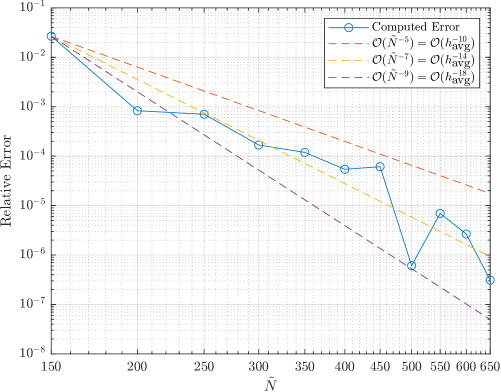
Figure 1. Relative error for the nearest computed Laplace–Beltrami eigenvalue to $\lambda=56$ using $\tilde{N}$ scattered points on the unit sphere. $h_{\text{avg}}$ is the average point spacing, which scales as $\mathcal{O}\left(\tilde{N}^{-\frac{1}{2}}\right)$ on a 2D surface

Note that the point generation is partially random, so we expect some irregularities in the convergence results, as seen in Fig. 1. The overall convergence appears to be high-order. For the $\tilde{N}=650$ test, we list the first 14 computed non-zero eigenvalues (not including multiplicities) along with their true values in Table 1. The computed eigenvalue corresponding to the true eigenvalue $\lambda=0$ was $10^{-8}$; Newton’s method was run to a tolerance of $10^{-8}$. Note that $\lambda=210$ is the 197th to 225th eigenvalue when multiplicities are included.

Table 1. First 14 non-zero eigenvalues on the unit sphere computed via minimization of $\left\|u_{\lambda}^{\left(\tilde{N}\right)}\right\|_{\mathcal{H}}^{2}$ with $\tilde{N}=650$ compared with the true eigenvalues and the corresponding relative error

Computed $\lambda$	True $\lambda$	Relative Error
1.99999999	2	5.7728E-09
5.99999996	6	7.3495E-09
11.99999973	12	2.2910E-08
19.99999965	20	1.7479E-08
29.99999981	30	6.3052E-09
41.99998409	42	3.7875E-07
55.99998263	56	3.1010E-07
71.99981050	72	2.6319E-06
89.99979568	90	2.2702E-06
109.99830299	110	1.5427E-05
131.99507487	132	3.7312E-05
155.97416335	156	1.6562E-04
181.88803616	182	6.1519E-04
209.75390413	210	1.1719E-03

These tests show that knowing $\left\|u_{\lambda}^{\left(\tilde{N}\right)}\right\|_{\mathcal{H}}^{2}$ is bounded if and only if $\lambda$ is an eigenvalue is sufficient for computing Laplace–Beltrami eigenvalues on an unstructured point cloud. Furthermore, estimates for the smaller eigenvalues are highly accurate, even for a fairly large point spacing ($\tilde{N}=650$ roughly corresponds to a distance on the order of $10^{-1}$ between points, on average).

4.2. Laplace–Beltrami on a Genus 2 Surface

Implicitly-defined surfaces generally do not have a parametrization available and may be difficult or expensive to mesh. Conversely, forming a point cloud on an implicit surface, as needed for our method, is relatively straightforward. For an example of a more complicated surface, we take a genus 2 surface defined as the zero set of the function:

$$\varphi\left(x,y,z\right):=\frac{1}{4\left(\left(x-1\right)^{2}+y^{2}\right)}+\frac{1}{4\left(\left(x+1\right)^{2}+y^{2}\right)}+\frac{1}{10}x^{2}+\frac{1}{4}y^{2}+z^{2}-1.$$

The point cloud is again generated using the algorithm in A.1 with $\tilde{N}_{\text{test},\partial}=40$. To better understand the method, it is helpful to examine a plot of $\left\|u_{\lambda}^{\left(\tilde{N}\right)}\right\|_{\mathcal{H}}$ as a function of $\lambda$; this is shown in Fig. 2. We use a Hilbert space given by Eq. (4.6) and a choice of $d_{n}$ given by Eq. (4.7) with parameters $q=5$ and $T=12$. $N_{b}=\left(2\cdot 15+1\right)^{3}$ Fourier basis functions on the box $\Omega=\left[-5,5\right]\times\left[-3,3\right]\times\left[-1.5,1.5\right]$ are used for the tests in this subsection.

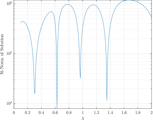
Figure 2. $\left\|u_{\lambda}^{\left(\tilde{N}\right)}\right\|_{\mathcal{H}}$ as a function of $\lambda$ for $\tilde{N}=1200$ for a genus 2 surface

Fig. 2 shows four clear minima of $\left\|u_{\lambda}^{\left(\tilde{N}\right)}\right\|_{\mathcal{H}}$ for $\lambda\in\left(0.1,2\right)$; these should correspond to eigenvalues of the Laplace–Beltrami operator on this surface. We test the convergence of the minima near $\lambda=0.3$ in Table 2, computed using Newton’s method initialized at 0.3 and run for 20 iterations or to an absolute tolerance of $10^{-12}$. We conclude that the first non-zero eigenvalue is around $0.3025$ or $0.3026$. Table 3 gives estimates of the second non-zero eigenvalue; it is around 0.6263 or 0.6264. In both tests, we observe convergence of the first few digits with point spacing on the order of $10^{-1}$. The eigenfunction corresponding to $\lambda\approx 0.626$ is shown in Fig. 3.

Table 2. First non-zero eigenvalue estimate for a genus two surface

$\tilde{N}$	Computed $\lambda$	Relative Change
400	0.3098406	N/A
800	0.3022492	2.5116E-02
1200	0.3025654	1.0452E-03
1600	0.3025519	4.4573E-05

Table 3. Second non-zero eigenvalue estimate for a genus two surface

$\tilde{N}$	Computed $\lambda$	Relative Change
800	0.6274113	N/A
1200	0.6264340	1.5601E-03
1600	0.6263515	1.3165E-04

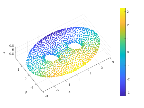
Figure 3. The Laplace–Beltrami eigenfunction corresponding to $\lambda\approx 0.626$ for a genus 2 surface, computed with $\tilde{N}=1600$ points

An alternative approach, for when the mean curvature of the surface is readily available, is to include the first normal derivative term in Laplace–Beltrami computation directly. That is, instead of using Eq. (4.5), we instead solve the following optimization problem:

(4.8) $$\text{minimize, over }u\in\mathcal{H}:\, \left\|u\right\|_{\mathcal{H}},$$

$$\text{subject to }:\, \left(-\Delta u+\hat{\boldsymbol{n}}_{S}\cdot\left(D^{2}u\right)\hat{\boldsymbol{n}}_{S}+\kappa\hat{\boldsymbol{n}}_{S}\cdot\nabla u\left(\boldsymbol{x}_{j}\right)-\lambda u\right)\left(\boldsymbol{x}_{j}\right)$$

$$\quad=0\text{, for $j\in\left\{1,2,\ldots,\tilde{N}\right\}$},$$

$$u\left(\boldsymbol{a}_{j}\right)=b_{j}\text{, for }j\in\left\{1,2,\ldots\tilde{N}_{a}\right\},$$

where $\kappa=\nabla\cdot\frac{\nabla\varphi}{\left\|\nabla\varphi\right\|_{2}}$. This approach uses Lemma 5 more directly and is numerically advantageous since it imposes fewer conditions. However, it is only applicable when $\kappa$ can be computed. In this case, $\kappa$ is known since we have a level set for the surface, but it is possible to estimate $\kappa$ accurately using only point cloud data via meshfree interpolation of a (local) level set. Methods for fitting level sets through unorganized points (thus computing normal vectors and mean curvature) are prevalent in the computer graphics community (see [6], for example); we take normal vectors as given throughout this paper and mean curvature as given for the rest of this subsection. Estimates of the first two non-zero eigenvalues using the approach from (4.8) are given in Tables 4 and 5. We note considerable improvement. Computation time is also significantly reduced since the matrices involved are smaller.

Table 4. First non-zero eigenvalue estimate for a genus two surface using the modified approach given by Eq. (4.8)

$\tilde{N}$	Computed $\lambda$	Relative Change
400	0.3019843	N/A
800	0.3025272	1.7948E-03
1200	0.3025111	5.3416E-05
1600	0.3025207	3.1804E-05
2000	0.3025205	7.2296E-07

Table 5. Second non-zero eigenvalue estimate for a genus two surface using the modified approach given by Eq. (4.8)

$\tilde{N}$	Computed $\lambda$	Relative Change
400	0.6265373	N/A
800	0.6262142	5.1589E-04
1200	0.6263335	1.9035E-04
1600	0.6263370	5.7036E-06
2000	0.6263408	6.0671E-06

4.3. Steklov Eigenvalues

For a domain with boundary $S$, the Steklov problem (for the Laplacian) is given by

$$\Delta u =0\text{ on }S,$$

$$\left(\hat{\boldsymbol{n}}\cdot\nabla u-\lambda u\right)\biggr{|}_{\partial S} =0.$$

That is, the eigenvalue $\lambda$ is in the boundary condition, not in the interior of the domain. A variety of methods have been proposed for this problem; primarily, these are finite element [18, 22, 31, 32, 35] or boundary integral methods [1, 9]. Adapting this problem for surfaces, which we do later in Subsection 4.6, is typically difficult. This is particularly true for boundary integral methods, since Green’s functions for the surface may not be known or feasible to compute, except for certain simple surfaces such as the sphere [16]. Boundary integral methods also rely on the availability of a suitable quadrature scheme, which also might not be available for surfaces. Also, as usual, meshing is more difficult on surfaces than for flat domains. A meshfree method for this problem could therefore be quite useful, especially on surfaces.

A major advantage of our approach is that it is completely universal for linear PDEs; there are no additional complications from a Steklov problem compared to the usual Laplace eigenvalue problem. We consider:

(4.9) $$\text{minimize, over }u\in\mathcal{H}: \left\|u\right\|_{\mathcal{H}},$$

$$\text{subject to }: \left(\Delta u\right)\left(\boldsymbol{x}_{j}\right)=0\text{, for each $j\in\left\{1,2,\ldots,\tilde{N}\right\}$},$$

$$\hat{\boldsymbol{n}}_{S}\cdot\nabla u\left(\boldsymbol{y}_{j}\right)-u\left(\boldsymbol{y}_{j}\right)=0\text{, for each }j\in\left\{1,2,\ldots\tilde{N}\right\},$$

$$u\left(\boldsymbol{a}_{j}\right)=1\text{, for each }j\in\left\{1,2,\ldots\tilde{N}_{a}\right\}.$$

As a test example, we examine this problem for the unit disk. The true Steklov eigenvalues for this problem are known to be the non-negative integers (see, for example, Example 1.3.1. of [17]). A note for the Steklov problem is that solutions are known to decay rapidly away from the boundary (see Thm. 1.1 of [20]); for this reason, it makes sense to place the $\boldsymbol{a}_{j}$ points on the boundary. This approach is more successful numerically than placing $\boldsymbol{a}_{j}$ points near the centre and is supported by the analysis of Subsection 3.3, which requires $\boldsymbol{a}_{j}$ to be on the boundary. We set $u\left(\boldsymbol{a}_{j}\right)=1$ on one point on the boundary ($\tilde{N}_{a}=1$), and use $N_{b}=\left(2\cdot 75+1\right)^{2}$, $\Omega=\left[-2,2\right]^{2}$, $q=4$, and $T=1$, with $\mathcal{H}$ as in Subsection 4.1, so that $d_{n}$ is given by Eq. (4.7) (where $\boldsymbol{\omega}_{n}$ is now in $\mathbb{R}^{2}$ rather than $\mathbb{R}^{3}$).

We take $\tilde{N}\approx\left(\frac{\tilde{N}_{\partial}}{4}\right)^{2}$, with more scattered points near the boundary than in the middle of the domain; this is done through a similar process as the point cloud in the previous subsection, but by weighting distances from the existing point cloud by $4\left(1-r^{2}\right)+1$, where $r$ is the distance of a potential new point from the origin. This gives a preference for points near the boundary, which we have observed numerically to improve convergence. The specific processes used are given in A.1 for the $\tilde{N}_{\partial}$ points on the boundary and A.2 for the $\tilde{N}$ points in the interior, with $w=4$. As an initial test, we search for the $\lambda=10$ Steklov eigenvalue at various resolutions. The result is shown in Fig. 4.

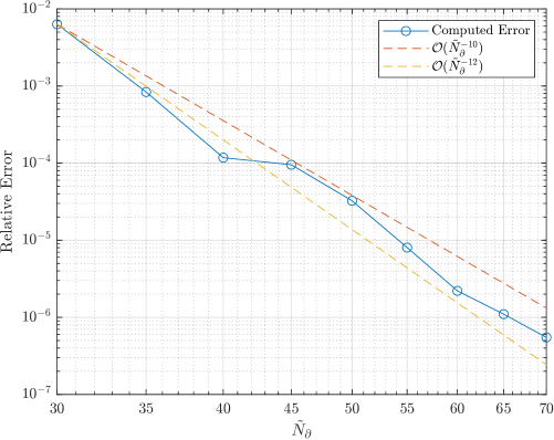
Figure 4. Relative error for the nearest computed Steklov eigenvalue to $\lambda=10$ using $\tilde{N}_{\partial}$ scattered points on the boundary of the unit disk and $\approx\tilde{N}_{\partial}/4$ points in the interior

Also, with $\tilde{N}_{\partial}=65$, we list the first 20 computed Steklov eigenvalues in Table 6, not including multiplicities. We capture the first 20 eigenvalues fairly accurately (39 including multiplicity); the behaviour is similar to the Laplace–Beltrami test from the previous subsection, demonstrating the generality of the method.

Table 6. First 20 Steklov eigenvalues on the unit disk computed via minimization of $\left\|u_{\lambda}^{\left(\tilde{N}\right)}\right\|_{\mathcal{H}}^{2}$ with $\tilde{N}_{\partial}=65$ compared with the true eigenvalues and the corresponding relative error

Computed $\lambda$	True $\lambda$	Relative Error
0.00000003	0	N/A
1.00000006	1	6.2890E-08
2.00000016	2	8.0386E-08
3.00000017	3	5.6464E-08
4.00000035	4	8.8185E-08
5.00000063	5	1.2542E-07
6.00000124	6	2.0704E-07
7.00000250	7	3.5761E-07
8.00000365	8	4.5586E-07
9.00000792	9	8.8046E-07
10.00000629	10	1.1014E-06
11.00001111	11	2.6668E-06
12.00003097	12	3.8164E-06
13.00006904	13	7.6722E-06
14.00011946	14	1.3818E-05
15.00016283	15	1.8485E-05
16.00023640	16	2.9443E-05
17.00031687	17	5.7753E-05
18.00072965	18	6.4974E-05
19.00131658	19	9.6579E-05

4.4. Exceptional Steklov–Helmholtz

An advantage of this approach is that we can handle problems that may be difficult with standard methods without any modifications. Consider a Steklov–Helmholtz problem on the unit disk:

$$-\Delta u-\mu^{2}u =0\text{ on }S,$$

$$\left(\hat{\boldsymbol{n}}\cdot\nabla u-\lambda u\right)\biggr{|}_{\partial S} =0.$$

A possible complication arises when $-\mu^{2}$ is an eigenvalue of the Laplacian with homogeneous Dirichlet boundary conditions. In this case, there is a Steklov “eigenvalue” $\lambda$ at $-\infty$ associated with the Dirichlet eigenfunction(s); as $\lambda\to-\infty$, the $\left(\hat{\boldsymbol{n}}\cdot\nabla u-\lambda u\right)\biggr{|}_{\partial S}=0$ condition becomes $u\biggr{|}_{\partial S}=0$. When $-\mu^{2}$ is close to a Dirichlet eigenvalue (as is the case numerically due to finite precision), there can instead be a large, negative Steklov eigenvalue. This can introduce numerical instability for some methods, even for low-resolution computations. Our method uses different matrices for each value of $\lambda$ (that can be formed from blocks of the same, more computationally intensive matrices) and only tests solvability for a specific $\lambda$, so it should not be affected by this issue.

To test this, we use $\mu=2.404825557695773$, which could cause the aforementioned problem since $-\mu^{2}$ is a Dirichlet eigenvalue in this case. We estimate the first positive Steklov–Helmholtz eigenvalue in Table 7, using the same parameters as the previous subsection. We do not encounter any issues; there is nothing unique about the Dirichlet eigenvalues for our method. Convergence in Table 7 is somewhat irregular, which is likely due to randomness in the point cloud generation process.

Table 7. Estimated first positive Steklov–Helmholtz eigenvalue on the unit disk, with $\mu=2.404825557695773$. The true value is $\approx 0.891592981473392$. The convergence rate is the negative slope of the log-log plot of relative error plotted against $\tilde{N}_{\partial}$

$\tilde{N}_{\partial}$	$\lambda$ Estimate	Relative Error	Convergence
18	0.914785095121278	2.6012E-02	N/A
30	0.891663966985981	7.9616E-05	11.333
42	0.891598053856290	5.6891E-06	7.842
54	0.891593063597904	9.2110E-08	16.407
66	0.891593015978842	3.8701E-08	4.321
78	0.891592981130651	3.8441E-10	27.607

4.5. Schrödinger–Steklov

We now consider the same problem as in the previous two subsections but with a Schrödinger equation rather than $\Delta u=0$ or $-\Delta u-\mu^{2}u=0$. That is, we consider

$$-\Delta u+qu =0\text{ on }S,$$

$$\left(\hat{\boldsymbol{n}}\cdot\nabla u-\lambda u\right)\biggr{|}_{\partial S} =0,$$

where $q$ is a given function on $S$ (physically, it is the potential energy). In [26], Quiñones computes asymptotic expressions for the Steklov eigenvalues $\lambda$ in the case that $S$ is the unit circle and $q$ is radial. These asymptotic expressions are compared to numerically obtained eigenvalues computed by Quiñones using a finite element method (FEM) based on code from Bogosel (Section 6 of [5]). One of the radial functions considered by Quiñones is

$$q\left(r\right)=\frac{\frac{1}{2}r+\frac{1}{5}\cos\left(5r\right)}{2r^{3}+1};$$

the 10th non-zero eigenvalue with this function was computed to be $\approx 10.00807486$ (Table 2.2 of [26]). We repeat this finite element computation using Bogosel’s code, modified for the Schrödinger–Steklov problem, and compare convergence to our meshfree approach. Table 8 shows a convergence test with all parameters identical to Subsection 4.3, as well as convergence for the P2 finite element method as a comparison. The convergence rates given in Table 8 are relative to $\tilde{N}_{\partial}$, which is inversely proportional to point spacing and element size, for the meshfree and FEM approaches, respectively.

Table 8. Schrödinger–Steklov eigenvalue $\lambda\approx 10.00807486$ computed via minimization of $\left\|u_{\lambda}^{\left(\tilde{N}\right)}\right\|_{\mathcal{H}}^{2}$ (meshfree, left) compared to a FEM computation with P2 elements (right). The convergence rate is the negative slope of the log-log plot of relative error plotted against $\tilde{N}_{\partial}$

Meshfree Method					FEM P2 (Adapted from [5])
$\tilde{N}_{\partial}$	$\tilde{N}$	Relative Error	Convergence		$\tilde{N}_{\partial}$	Vertices	Relative Error	Convergence
30	225	6.3316E-03	N/A		100	922	6.4788E-04	N/A
40	400	1.1775E-04	13.851		200	3592	7.5038E-05	3.110
50	625	3.2597E-05	5.756		400	14002	1.2373E-05	2.600
60	900	2.2297E-06	14.712		800	55300	2.6978E-06	2.197
70	1225	6.1868E-07	8.317		1600	220477	6.4948E-07	2.054

Given that our method converges super-algebraically in theory, the much faster observed convergence rate of the meshfree method is to be expected; we are able to obtain accurate results with far fewer points. Of course, this is at the cost of having a dense matrix, but with the added benefit of being completely meshfree.

4.6. Surface Steklov

A useful aspect of our approach is that the same method applies to surface PDEs. This is not the case for various other high-order Steklov eigenvalue approaches that may require a Green’s function, which are often not readily available for surfaces. We also do not require the surface’s metric or any quadrature scheme to be implemented; only a point cloud and (unoriented) normal vectors on the point cloud are needed.

We study a catenoid with a “wavy” edge, given by the parametrization:

$$\sigma\left(s,t\right)=\left(\cosh\left(t\right)\cos\left(s\right),\cosh\left(t\right)\sin\left(s\right),t\right),$$

for $s\in\left[0,2\pi\right)$ and $-1+0.1\sin\left(3s\right)\leq t\leq 1+0.1\sin\left(3s\right)$. The Steklov problem on this surface is

$$\Delta_{S}u =0\text{ on }S,$$

$$\left(\hat{\boldsymbol{\nu}}\cdot\nabla_{S}u-\lambda u\right)\biggr{|}_{\partial S} =0,$$

where $\hat{\boldsymbol{\nu}}$ is the outward normal to $\partial S$ (perpendicular to the tangent vector to $\partial S$ and the normal vector $\hat{\boldsymbol{n}}_{S}$ to $S$). This is discretized very similarly to the examples in Subsections 4.1-4.3:

(4.10) $$\text{minimize, over }u\in\mathcal{H}: \left\|u\right\|_{\mathcal{H}},$$

$$\text{subject to }: \left(-\Delta u+\hat{\boldsymbol{n}}_{S}\cdot\left(D^{2}u\right)\hat{\boldsymbol{n}}_{S}\right)\left(\boldsymbol{x}_{j}\right)=0\text{, for each $j\in\left\{1,2,\ldots,\tilde{N}\right\}$},$$

$$\hat{\boldsymbol{n}}_{S}\cdot\nabla u\left(\boldsymbol{x}_{j}\right)=0\text{, for each }j\in\left\{1,2,\ldots\tilde{N}\right\},$$

$$\hat{\boldsymbol{n}}_{S}\cdot\nabla u\left(\boldsymbol{y}_{j}\right)=0\text{, for each }j\in\left\{1,2,\ldots\tilde{N}_{\partial}\right\},$$

$$\left(\hat{\boldsymbol{\nu}}\cdot\nabla u\left(\boldsymbol{y}_{j}\right)-\lambda u\left(\boldsymbol{y}_{j}\right)\right)=0\text{, for each }j\in\left\{1,2,\ldots\tilde{N}_{\partial}\right\},$$

$$u\left(\boldsymbol{a}_{j}\right)=1\text{, for each }j\in\left\{1,2,\ldots\tilde{N}_{a}\right\}.$$

We seek to estimate the first non-zero eigenvalue. This is again done via minimization of $\left\|u_{\lambda}^{\left(\tilde{N}\right)}\right\|_{\mathcal{H}}^{2}$ as a function of $\lambda$. As it turns out, we see numerically that the first eigenvalue is close to 0.46, so we initialize higher accuracy tests starting at 0.46 before using Newton’s method to approximately find the minimum. We use $q=4$, $T=\tilde{\ell}=5$, and $\tilde{N}_{a}=1$. $\tilde{N}_{\partial}$ is the total number of points on the boundaries, so there are $\tilde{N}_{\partial}/2$ points on each of the two curves of $\partial S$. The eigenvalue estimates for various $\tilde{N}_{\partial}$ (inversely proportional to $h_{\text{max}}$) are in Table 9, along with the change between subsequent tests. We observe convergence to 5 or 6 digits of accuracy with $\tilde{N}_{\partial}=126$.

Table 9. Steklov eigenvalue $\lambda\approx 0.46506$ computed via minimization of $\left\|u_{\lambda}^{\left(\tilde{N}\right)}\right\|_{\mathcal{H}}^{2}$ and the difference between subsequent tests

$\tilde{N}_{\partial}$	$\lambda$ Estimate	Relative Change
66	0.4651428	N/A
78	0.4650323	2.3756E-04
90	0.4650468	3.1173E-05
102	0.4650578	2.3630E-05
114	0.4650583	9.7921E-07
126	0.4650585	4.6812E-07

4.7. Multiplicity

We have seen how Proposition 2 can be used to find eigenvalues. With standard methods, eigenvalues of differential operators are estimated as the eigenvalues of a matrix used to discretize the differential operator. Such approaches can produce repeated eigenvalues, which often correctly indicate the multiplicities of the eigenvalues of the differential operator. In our approach, we simply see minima of a function in $\mathbb{R}$ or $\mathbb{C}$. This leaves the problem of determining the multiplicity of eigenvalues.

With probability one, if the multiplicity of an eigenvalue $\lambda$ is $n$, we expect to be able to interpolate $n$ random values at $n$ random points with an eigenfunction with eigenvalue $\lambda$. We can then consider the problem on a surface $S$:

$$\left(-\Delta_{S}u-\lambda u\right) =0\text{ on }S,$$

$$u\left(\boldsymbol{a}_{j}\right) =b_{j}\text{, for each }j\in\left\{1,2,\ldots\tilde{N}_{a}\right\}.$$

Now, if the points $\left\{\boldsymbol{a}_{j}\right\}$ and values $\left\{b_{j}\right\}$ are selected at random, we expect this to be solvable (with probability one) only when $\lambda$ is an eigenvalue of $\Delta_{S}$ with multiplicity at least $\tilde{N}_{a}$. There are a number of ways to use this fact. On a surface, the discretized version of our problem is given by (4.5) from earlier. If $u_{\lambda,\tilde{N}_{a}}^{\left(\tilde{N}\right)}$ now represents the solution to (4.5) with $\tilde{N}_{a}$ randomly selected points $\left\{\boldsymbol{a}_{j}\right\}$ and values $\left\{b_{j}\right\}$, we expect $\left\|u_{\lambda,\tilde{N}_{a}}^{\left(\tilde{N}\right)}\right\|_{\mathcal{H}}$ to only remain bounded as $\tilde{N}\to\infty$ when $\lambda$ is an eigenvalue with multiplicity at least $\tilde{N}_{a}$. We demonstrate this for the sphere in Fig. 5, where $\left\|u_{\lambda,\tilde{N}_{a}}^{\left(\tilde{N}\right)}\right\|_{\mathcal{H}}$ is plotted as a function of $\lambda$ for $\tilde{N}_{a}=1,3,$ and 5, using the same parameters as Subsection 4.1.

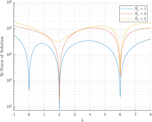
Figure 5. $\left\|u_{\lambda,\tilde{N}_{a}}^{\left(\tilde{N}\right)}\right\|_{\mathcal{H}}$ plotted against $\lambda$ to test for eigenvalue multiplicities, using $\tilde{N}_{a}=1,3,5$. $\tilde{N}=400,N_{b}=\left(2\cdot 15+1\right)^{3},\Omega=\left[-2,2\right]^{3},q=4$, and $T=4$, with the same $\mathcal{H}$ as Subsection 4.1

Visually, we see that there are sharp minima when $\lambda$ is an eigenvalue and it has multiplicity of at least $\tilde{N}_{a}$. In this example, $\lambda=0$ has multiplicity 1, $\lambda=2$ has multiplicity $3$, and $\lambda=6$ has multiplicity $5$. However, we see from the plot that for $\tilde{N}_{a}=5$, there may be another minimum of $\left\|u_{\lambda,\tilde{N}_{a}}^{\left(\tilde{N}\right)}\right\|_{\mathcal{H}}$ somewhere between $\lambda=1$ and $\lambda=2$. This minimum does not look as sharp as the others, however, which motivates us to consider a more robust test of multiplicity that can correctly distinguish these two types of local minima. To do this, we use the limits from Equations (3.18) and (3.19). These limits are quite useful since they tell us that the ratio $\left\|u_{\lambda,\tilde{N}_{a}}^{\left(\tilde{N}_{2}\right)}\right\|_{\mathcal{H}}/\left\|u_{\lambda,\tilde{N}_{a}}^{\left(\tilde{N}_{1}\right)}\right\|_{\mathcal{H}}$ must go to either 1 or $\infty$, depending on whether the problem is solvable or not. Once we already have eigenvalue estimates using $\tilde{N}_{a}=1$, we can check their multiplicity using the norm ratio.

As a demonstration, we look at the $\lambda=56$ eigenvalue for the Laplace–Beltrami operator on the unit sphere, which has multiplicity 15. We give the norm ratio $\left\|u_{\lambda,\tilde{N}_{a}}^{\left(\tilde{N}_{2}\right)}\right\|_{\mathcal{H}}/\left\|u_{\lambda,\tilde{N}_{a}}^{\left(\tilde{N}_{1}\right)}\right\|_{\mathcal{H}}$ for $\lambda=56$ and multiplicities 14-17 in Table 10. We use $\tilde{N}_{2}\approx\frac{10}{9}\tilde{N}_{1}$ and the same $\mathcal{H}$ as in the previous test. The expected behaviour is observed, and by the last test, the true multiplicity is fairly clearly indicated. That is, the norm ratio for $\tilde{N}_{a}=15$ is approaching 1, while the norm ratio for $\tilde{N}_{a}=16$ appears to be diverging; the norm is still nearly doubling with each (fairly small) refinement. This indicates to us that it is likely possible to select a cutoff value for the ratio slightly higher than one, then consider a ratio less than that value to indicate an eigenvalue with at least multiplicity $\tilde{N}_{a}$.

Table 10. Norm ratio $\left\|u_{\lambda,\tilde{N}_{a}}^{\left(\tilde{N}_{2}\right)}\right\|_{\mathcal{H}}/\left\|u_{\lambda,\tilde{N}_{a}}^{\left(\tilde{N}_{1}\right)}\right\|_{\mathcal{H}}$for $\lambda=56$ (multiplicity 15) and various $\tilde{N}_{1}$ values, with $\tilde{N}_{2}\approx\frac{10}{9}\tilde{N}$

		14	15	16	17
400		1.0112	1.0496	1.0897	1.4007
500		1.0026	1.0628	1.2488	1.3880
600		1.0005	1.0350	1.7106	1.6857
700		1.0001	1.0073	1.6638	1.7111
800		1.0000	1.0026	1.9056	2.1866

Using $\tilde{N}_{2}\approx\frac{10}{9}\tilde{N}_{1}$, we also test the multiplicity of the $\lambda=156$ eigenvalue in Table 11. $\tilde{N}_{1}=900$ or $1000$ offers sufficient resolution for us to observe that the ratio is approaching 1 for $\tilde{N}_{a}=25$, but increasing for $\tilde{N}_{a}=26$. Note that this test covers the 625th eigenvalue, including multiplicity.

Table 11. Norm ratio $\left\|u_{\lambda,\tilde{N}_{a}}^{\left(\tilde{N}_{2}\right)}\right\|_{\mathcal{H}}/\left\|u_{\lambda,\tilde{N}_{a}}^{\left(\tilde{N}_{1}\right)}\right\|_{\mathcal{H}}$for $\lambda=156$ (multiplicity 25) and various $\tilde{N}_{1}$ values, with $\tilde{N}_{2}\approx\frac{10}{9}\tilde{N}$

	24	25	26	27
400	1.1397	1.1473	1.1501	1.1509
500	1.2410	1.2385	1.2933	1.3034
600	1.2108	1.2349	1.3843	1.3566
700	1.1598	1.2182	1.5749	1.5796
800	1.0979	1.2434	1.8705	1.8795
900	1.0277	1.0811	2.0428	2.1348
1000	1.0074	1.0232	2.2747	2.2875

5. Conclusions

We presented a very general result (Proposition 2) detailing how the boundedness of Hermite–Birkhoff interpolants in certain Hilbert spaces is necessary and sufficient for solutions to linear PDEs to exist in a very general context, and we explained how this could be used to determine the solvability of linear PDEs. In Propositions 3 and 4, we proved inequalities that show the high-order convergence of our approach for estimating eigenvalues and eigenfunctions. Then, we tested our method numerically for a variety of problems and observed the rapid convergence of eigenvalue estimates. Notably, we are able to handle surface PDEs, problems with varying coefficients, and Steklov problems all with the same approach.

Our method has certain advantages; we see its universality for linear PDEs as its primary advantage, as well as its meshfree nature. Propositions 2, 3, and 4 show analytically that the method produces correct eigenvalues with no spurious modes, and show that the method converges at a high-order rate for suitable problems. We also observe that our method is numerically reliable for producing correct eigenvalues at high enough point densities, and that estimates converge extremely quickly. This differs from other high-order, meshfree methods that have been used for solving PDEs, but lack analytical convergence results for eigenvalue estimates and do not reliably produce the correct eigenvalues without spurious modes in practice. Meshfree methods are highly desirable for surface PDEs due to the difficulty of mesh creation. It is generally much easier to produce a point cloud than a mesh for irregularly shaped flat domains and surfaces. In practice, surfaces may also be defined by a point cloud originating from a scan of an object, which requires a large amount of pre-processing to mesh.

Extensions of this work may focus on scaling up the method to solve larger problems. There are Hilbert spaces with useful basis functions properties (compact support, separable, etc.) that can be used to greatly decrease computational costs. In other work, we are investigating Hilbert spaces that produce $\psi_{j}$ functions that vary by location, which may help substantially in capturing fine details where necessary without substantially increasing the point density for the whole domain. This may help with a key weakness of standard global RBF methods, where narrower basis functions cannot be used without high point densities for the entire domain. We are also exploring using Proposition 2 for other problems regarding PDE solvability, such as inverse problems, and using known PDE solvability conditions that depend on integrals to develop accurate meshfree integration techniques on surfaces.

Acknowledgements

We acknowledge the support of the Natural Sciences and Engineering Research Council of Canada (NSERC), [funding reference number RGPIN 2022-03302].

Appendix A Point Cloud Generation Algorithms

A.1. Boundary Algorithm for Curves and Surfaces

Let $\tilde{N}_{\partial}$ be the desired number of points on the boundary $\partial U$ of an open set $U$.

1. Create $\tilde{N}_{\text{test},\partial}>\tilde{N}_{\partial}$ points on the boundary: $\left\{\boldsymbol{z}_{j}\right\}_{j=1}^{\tilde{N}_{\text{test},\partial}}$. If the boundary is defined by a level set, this can be achieved by placing points in a larger set containing $\partial U$, then using Newton’s method or another root-finding algorithm to move the points onto $\partial U$. That is, if $\partial U:=\left\{\boldsymbol{x}\in\mathbb{R}^{m}:\varphi\left(\boldsymbol{x}\right)=0\right\}$, we can initialize a root-finding algorithm at a point $\tilde{\boldsymbol{z}}_{j}$ near $\partial U$ to find some $\boldsymbol{z}_{j}\in\partial U$ such that $\varphi\left(\boldsymbol{z}_{j}\right)=0$.

2. Add one point to the boundary point cloud from the $\tilde{N}_{\text{test},\partial}$ points. Call it $\boldsymbol{y}_{1}$.

3. If the boundary point cloud has $k$ points, $\left\{\boldsymbol{y}_{j}\right\}_{j=1}^{k}$, choose $\boldsymbol{y}_{k+1}$ to be the point in $\left\{\boldsymbol{z}_{j}\right\}_{j=1}^{\tilde{N}_{\text{test},\partial}}$ farthest away from $\left\{\boldsymbol{y}_{j}\right\}_{j=1}^{k}$ (simply using the Euclidean norm in the embedding space: $\left\|\cdot\right\|_{2}$).

4. Repeat the previous step until there are $\tilde{N}_{\partial}$ points in the point cloud: $\left\{\boldsymbol{y}_{j}\right\}_{j=1}^{\tilde{N}_{\partial}}$.

A.2. Interior Algorithm

Let $U\subset\mathbb{R}^{m}$ be open and defined by a level set $U:=\left\{\boldsymbol{x}\in\mathbb{R}^{m}:\varphi\left(\boldsymbol{x}\right)<0\right\}$, and let the minimum value of $\varphi$ on $\overline{U}$ be $a$.

1. Start with an empty point cloud.

2. Create $\tilde{N}_{\text{test}}$ points in $U$: $\left\{\boldsymbol{z}_{j}\right\}_{j=1}^{\tilde{N}_{\text{test}}}$.

3. If the point cloud currently has $k$ points, $\left\{\boldsymbol{x}_{j}\right\}_{j=1}^{k}$, choose $\boldsymbol{x}_{j}$ to be the point in $\left\{\boldsymbol{z}_{j}\right\}_{j=1}^{\tilde{N}_{\text{test}}}$ with the largest penalty, where the penalty is defined by

   $$P_{k}\left(\boldsymbol{z}\right)=\left(w\left(1-\frac{\varphi\left(\boldsymbol{z}\right)}{a}\right)+1\right)\min\left\{\left\|\boldsymbol{x}-\boldsymbol{z}\right\|_{2}^{2}:\boldsymbol{x}\in\left\{\boldsymbol{x}_{j}\right\}_{j=1}^{k}\cup\left\{\boldsymbol{y}_{j}\right\}_{j=1}^{\tilde{N}_{\partial}}\right\},$$

   where $w$ is a parameter that controls preference for placing points near the boundary.

4. Repeat steps 2 and 3 until the point cloud has $\tilde{N}$ points.

References

- [1] Eldar Akhmetgaliyev, Chiu-Yen Kao and Braxton Osting “Computational methods for extremal Steklov problems” In SIAM J. Control Optim. 55.2 SIAM, 2017, pp. 1226–1240 DOI: 10.1137/16M1067263
- [2] Diego Álvarez, Pedro González-Rodríguez and Manuel Kindelan “A local radial basis function method for the Laplace–Beltrami operator” In J. Sci. Comput. 86.3 Springer, 2021, pp. 28 DOI: 10.1007/s10915-020-01399-3
- [3] Stefan Auer et al. “Real-time fluid effects on surfaces using the closest point method” In Computer Graphics Forum 31.6, 2012, pp. 1909–1923 Wiley Online Library DOI: 10.1111/j.1467-8659.2012.03071.x
- [4] Harry Biddle, Ingrid Glehn, Colin B. Macdonald and Thomas März “A volume-based method for denoising on curved surfaces” In 2013 IEEE International Conference on Image Processing, 2013, pp. 529–533 DOI: 10.1109/ICIP.2013.6738109
- [5] Beniamin Bogosel “The method of fundamental solutions applied to boundary eigenvalue problems” In J. Comput. Appl. Math. 306, 2016, pp. 265–285 DOI: https://doi.org/10.1016/j.cam.2016.04.008
- [6] J.. Carr et al. “Reconstruction and Representation of 3D Objects with Radial Basis Functions” In Proceedings of the 28th Annual Conference on Computer Graphics and Interactive Techniques, SIGGRAPH ’01 New York, USA: Association for Computing Machinery, 2001, pp. 67–76 DOI: 10.1145/383259.383266
- [7] S. Chandrasekaran and H.N. Mhaskar “A minimum Sobolev norm technique for the numerical discretization of PDEs” In J. Comput. Phys. 299, 2015, pp. 649–666 DOI: 10.1016/j.jcp.2015.07.025
- [8] Shivkumar Chandrasekaran, CH Gorman and Hrushikesh Narhar Mhaskar “Minimum Sobolev norm interpolation of scattered derivative data” In J. Comput. Phys. 365 Elsevier, 2018, pp. 149–172 DOI: 10.1016/j.jcp.2018.03.014
- [9] Jeng-Tzong Chen, Jia-Wei Lee and Kuen-Ting Lien “Analytical and numerical studies for solving Steklov eigenproblems by using the boundary integral equation method/boundary element method” In Eng. Anal. Boundary Elem. 114 Elsevier, 2020, pp. 136–147 DOI: 10.1016/j.enganabound.2020.02.005
- [10] Meng Chen and Leevan Ling “Exploring oversampling in RBF least-squares collocation method of lines for surface diffusion” In Numer. Algorithms Springer, 2024, pp. 1–21 DOI: 10.1007/s11075-023-01741-4
- [11] Meng Chen and Leevan Ling “Extrinsic Meshless Collocation Methods for PDEs on Manifolds” In SIAM J. Numer. Anal. 58.2, 2020, pp. 988–1007 DOI: 10.1137/17M1158641
- [12] Ka Chun Cheung, Leevan Ling and Robert Schaback “-Convergence of Least-Squares Kernel Collocation Methods” In SIAM J. Numer. Anal. 56.1 SIAM, 2018, pp. 614–633 DOI: 10.1137/16M1072863
- [13] L.C. Evans “Partial Differential Equations” 19, Graduate Studies in Mathematics Providence, USA: American Mathematical Society, 2010 DOI: 10.1090/gsm/019
- [14] Bengt Fornberg and Erik Lehto “Stabilization of RBF-generated finite difference methods for convective PDEs” In J. Comput. Phys. 230.6, 2011, pp. 2270–2285 DOI: https://doi.org/10.1016/j.jcp.2010.12.014
- [15] C. Franke and R. Schaback “Solving partial differential equations by collocation using radial basis functions” In Appl. Math. Comput. 93.1, 1998, pp. 73–82 DOI: 10.1016/S0096-3003(97)10104-7
- [16] Simon Gemmrich, Nilima Nigam and Olaf Steinbach “Boundary integral equations for the Laplace-Beltrami operator” In Mathematics and Computation, a Contemporary View: The Abel Symposium 2006 Proceedings of the Third Abel Symposium, Alesund, Norway, May 25–27, 2006, 2008, pp. 21–37 Springer DOI: 10.1007/978-3-540-68850-1˙2
- [17] Alexandre Girouard and Iosif Polterovich “Spectral geometry of the Steklov problem (survey article)” In J. Spectr. Theory 7.2, 2017, pp. 321–359 DOI: 10.4171/JST/164
- [18] Xiaole Han, Yu Li and Hehu Xie “A multilevel correction method for Steklov eigenvalue problem by nonconforming finite element methods” In Numer. Math. Theory Methods Appl. 8.3 Cambridge University Press, 2015, pp. 383–405 DOI: 10.4208/nmtma.2015.m1334
- [19] John Harlim, Shixiao Willing Jiang and John Wilson Peoples “Radial Basis Approximation of Tensor Fields on Manifolds: From Operator Estimation to Manifold Learning” In J. Mach. Learn. Res. 24.345, 2023, pp. 1–85 URL: http://jmlr.org/papers/v24/22-1193.html
- [20] Peter D Hislop and Carl V Lutzer “Spectral asymptotics of the Dirichlet-to-Neumann map on multiply connected domains in ” In Inverse Problems 17.6 IOP Publishing, 2001, pp. 1717–1741 DOI: 10.1088/0266-5611/17/6/313
- [21] E.J. Kansa “Multiquadrics—A scattered data approximation scheme with applications to computational fluid-dynamics—II Solutions to parabolic, hyperbolic and elliptic partial differential equations” In Comput. Math. with Appl. 19.8, 1990, pp. 147–161 DOI: 10.1016/0898-1221(90)90271-K
- [22] Qin Li, Qun Lin and Hehu Xie “Nonconforming finite element approximations of the Steklov eigenvalue problem and its lower bound approximations” In Appl. Math. 58.2 Springer, 2013, pp. 129–151 DOI: 10.1007/s10492-013-0007-5
- [23] William Charles Hector McLean “Strongly elliptic systems and boundary integral equations” Cambridge, UK: Cambridge University Press, 2000 DOI: 10.2307/3621632
- [24] Francis J. Narcowich, Joseph D. Ward and Holger Wendland “Sobolev Bounds on Functions with Scattered Zeros, with Applications to Radial Basis Function Surface Fitting” In Math. Comput. 74.250 American Mathematical Society, 2005, pp. 743–763 DOI: 10.1090/S0025-5718-04-01708-9
- [25] Ahmad Nasikun, Christopher Brandt and Klaus Hildebrandt “Fast Approximation of Laplace-Beltrami Eigenproblems” In Computer Graphics Forum 37.5, 2018, pp. 121–134 Wiley Online Library DOI: 10.1111/cgf.13496
- [26] Leoncio Rodriguez Quiñones “Direct and inverse problems for a Schrödinger-Steklov eigenproblem on different domains and spectral geometry for the first normalized Steklov eigenvalue on domains with one hole”, 2018
- [27] Martin Reuter, Franz-Erich Wolter and Niklas Peinecke “Laplace-Beltrami spectra as ‘Shape-DNA’ of surfaces and solids” In Comput.-Aided Des. 38.4 Elsevier, 2006, pp. 342–366 DOI: 10.1016/j.cad.2005.10.011
- [28] Xingping Sun “Scattered Hermite interpolation using radial basis functions” In Linear Algebra Appl. 207, 1994, pp. 135–146 DOI: 10.1016/0024-3795(94)90007-8
- [29] Daniel R Venn and Steven J Ruuth “Underdetermined Fourier Extensions for Partial Differential Equations on Surfaces” Preprint at https://arxiv.org/abs/2401.04328 (2024)
- [30] Holger Wendland “Scattered Data Approximation”, Cambridge Monographs on Applied and Computational Mathematics Cambridge, UK: Cambridge University Press, 2004 DOI: 10.1017/CBO9780511617539
- [31] Zhifeng Weng, Shuying Zhai and Xinlong Feng “An improved two-grid finite element method for the Steklov eigenvalue problem” In Appl. Math. Modell. 39.10-11 Elsevier, 2015, pp. 2962–2972 DOI: 10.1016/j.apm.2014.11.017
- [32] Chunguang Xiong, Manting Xie, Fusheng Luo and Hongling Su “A posteriori and superconvergence error analysis for finite element approximation of the Steklov eigenvalue problem” In Comput. Math. Appl. 144 Elsevier, 2023, pp. 90–99 DOI: 10.1016/j.camwa.2023.05.025
- [33] Jian-Jun Xu and Hong-kai Zhao “An Eulerian Formulation for Solving Partial Differential Equations Along a Moving Interface” In J. Sci. Comput. 19, 2003, pp. 573–594 DOI: 10.1023/A:1025336916176
- [34] Qile Yan, Shixiao Willing Jiang and John Harlim “Spectral methods for solving elliptic PDEs on unknown manifolds” In J. Comput. Phys. 486, 2023, pp. 112132 DOI: 10.1016/j.jcp.2023.112132
- [35] Chun’guang You, Hehu Xie and Xuefeng Liu “Guaranteed eigenvalue bounds for the Steklov eigenvalue problem” In SIAM J. Numer. Anal. 57.3 SIAM, 2019, pp. 1395–1410 DOI: 10.1137/18M1189592