Improving generalization with Flat Hilbert Bayesian Inference
Abstract
We introduce Flat Hilbert Bayesian Inference (FHBI), an algorithm designed to enhance generalization in Bayesian inference. Our approach involves an iterative two-step procedure with an adversarial functional perturbation step and a functional descent step within the reproducing kernel Hilbert spaces. This methodology is supported by a theoretical analysis that extends previous findings on generalization ability from finite-dimensional Euclidean spaces to infinite-dimensional functional spaces. To evaluate the effectiveness of FHBI, we conduct comprehensive comparisons against seven baseline methods on the VTAB-1K benchmark, which encompasses 19 diverse datasets across various domains with diverse semantics. Empirical results demonstrate that FHBI consistently outperforms the baselines by notable margins, highlighting its practical efficacy. Our code is available at https://anonymous.4open.science/r/Flat-Hilbert-Variational-Inference-008F/.
1 Introduction
Quantifying and tackling uncertainty in deep learning is one of the most challenging problems, mainly due to the inherent randomness of the real world and the presence of noisy data. Bayesian inference provides a robust framework for understanding complex data, allowing for probabilistic interpretation of deep learning models and reasoning under uncertainty. This approach not only facilitates predictions but also enables the quantification of uncertainty. A primary challenge in this domain is the computation and sampling from intricate distributions, mainly when dealing with deep learning models. One effective strategy to tackle this issue is variational inference, which seeks to approximate the true posterior distribution with simpler forms, known as approximate posteriors while optimizing a variational lower bound. Several techniques have been developed in this area, including those by Kingma & Welling (2013); Kingma et al. (2015), and Blundell et al. (2015), who extended the Gaussian variational posterior approximation for neural networks, as well as Gupta & Nagar (2018), who enhanced the flexibility of posterior approximations. In addition to variational methods, various particle sampling techniques have been proposed for Bayesian inference, especially in scenarios requiring multiple models. Notable particle sampling methods include Hamiltonian Monte Carlo (HMC) (Neal, 1996), Stochastic Gradient Langevin Dynamics (SGLD) (Welling & Teh, 2011), Stochastic Gradient HMC (SGHMC) (Chen et al., 2014), and Stein Variational Gradient Descent (SVGD) (Liu & Wang, 2016b). Each method contributes to a deeper understanding and more practical application of Bayesian inference in deep learning.
Besides quantifying uncertainty, tackling overfitting is a major challenge in machine learning. Overfitting often occurs when the training process gets stuck in local minima, leading to a model that fails to generalize well to unseen data. This problem is mainly due to loss functions’ high-dimensional and non-convex nature, which often exhibit multiple local minima in the loss landscape. In standard deep network training, flat minimizers effectively improve model generalization (Keskar et al., 2016; Kaddour et al., 2022; Li et al., 2022). Among the flat minimizers, Sharpness-Aware Minimization (SAM) (Foret et al., 2021) has emerged as a practical approach by concurrently minimizing the empirical loss and reducing the sharpness of the loss function. Recently, SAM has demonstrated its versatility and effectiveness across a wide range of tasks, including meta-learning (Abbas et al., 2022), federated learning (Qu et al., 2022), vision models (Chen et al., 2021), and language models (Bahri et al., 2022).
Contribution.
We bridge the gap between the flat minimizers and particle sampling to introduce a Bayesian inference framework with improved generalization ability. To accomplish this, we first present Theorem 1, which strengthens prior generalization bounds from finite-dimensional Euclidean spaces to the reproducing kernel Hilbert spaces (RKHS), which are broader and more general functional spaces that are typically infinite-dimensional. Notably, this theorem introduces the notion of functional sharpness that offers an insight to improve the generalization ability of current particle-sampling methods. Subsequently, Theorem 2 translates these notions of functional sharpness and generalization in RKHS into the context of Bayesian inference. This analysis establishes a connection between the general and empirical KL loss, providing a strategy to enhance generalization by minimizing the general KL loss. Motivated by these two theorems, we derive Flat Hilbert Bayesian Inference (FBVI), a practical algorithm that employs a dual-step functional sharpness-aware update procedure in RKHS. This approach improves the generalization of sampled particles, thereby enhancing the quality of the ensemble. Overall, our contributions are as follows:
-
1.
We present a theoretical analysis that characterizes generalization ability over the functional space. This analysis generalizes prior works from the Euclidean space to infinite-dimensional functional space, thereby introducing the notion of functional sharpness i.e., the sharpness of the functional spaces.
-
2.
Building on this theoretical foundation, we propose a practical particle-sampling algorithm that enhances the generalization ability over existing methods. We conducted extensive experiments comparing our Flat Hilbert Bayesian Inference (FHBI) algorithm with seven baselines on the VTAB-1K benchmark, which includes 19 datasets across various domains and semantics. Experimental results demonstrated that our algorithm outperforms these baselines by notable margins.
The paper is structured as follows: Section 2 reviews the related works on Bayesian inference and the development of flat minimizers. Section 3 provides the necessary background and notations. Section 4 discusses the motivation and theoretical development behind our sharpness-aware particle-sampling approach. Section 5 presents experimental results, comparing our algorithm against various Bayesian inference baselines across diverse settings. Section 6 offers a deeper analysis of FHBI’s behavior to gain further insight into its effectiveness over the baseline methods.
2 Related Works
Sharness-aware minimization.
Flat minimizers have been shown to be more robust to the shifts between training and test losses, thereby enhancing the generalization ability of neural networks (Jiang et al., 2020; Petzka et al., 2021; Dziugaite & Roy, 2017). The relationship between generalization and the width of minima has been studied both theoretically and empirically in several prior works (Hochreiter & Schmidhuber, 1994; Neyshabur et al., 2017; Dinh et al., 2017; Fort & Ganguli, 2019). Consequently, a variety of methods have been developed to search for flat minima (Pereyra et al., 2017; Chaudhari et al., 2017; Keskar et al., 2017; Izmailov et al., 2018).
Among the flat minizer, Sharpness-Aware Minimization (SAM), introduced by Foret et al. (2021), has gained significant attention due to its effectiveness and scalability. SAM’s versatility has been leveraged across a wide range of tasks and domains, including domain generalization (Cha et al., 2021; Wang et al., 2023; Zhang et al., 2023), federated learning (Caldarola et al., 2022; Qu et al., 2022), Bayesian networks (Nguyen et al., 2023; Möllenhoff & Khan, 2023), and meta-learning (Abbas et al., 2022). Moreover, SAM has demonstrated its ability to enhance generalization in both vision models (Chen et al., 2021) and language models (Bahri et al., 2022).
Nevertheless, these studies are constrained to finite-dimensional Euclidean spaces. In this work, we strengthen these generalization principles to infinite-dimensional functional spaces and propose a particle-sampling method grounded in this theoretical framework.
Bayesian Inference.
Two main strategies were widely employed in the literature of Bayesian inference. The first paradigm is Variational Inference, which aims to approximate a target distribution by selecting a distribution from a family of potential approximations and optimizing a variational lower bound. Graves (2011) introduced the use of a Gaussian variational posterior approximation for neural network weights, which was later extended in Kingma & Welling (2013); Kingma et al. (2015); Blundell et al. (2015) with the reparameterization trick to facilitate training deep latent variable models. Louizos & Welling (2017) proposed using a matrix-variate Gaussian to model entire weight matrices (Gupta & Nagar, 2018) to increase further the flexibility of posterior approximations, which offers a novel approach to approximate the posterior. Subsequently, various alternative structured forms of the variational Gaussian posterior were proposed, including the Kronecker-factored approximations (Zhang et al., 2018; Ritter et al., 2018; Rossi et al., 2020), or non-centered or rank-1 parameterizations (Ghosh et al., 2018; Dusenberry et al., 2020).
The second paradigm in the literature of Bayesian inference is Markov Chain Monte Carlo (MCMC), which involves sampling multiple models from the posterior distribution. MCMC has been applied to neural network inference, such as Hamiltonian Monte Carlo (HMC) (Neal, 1996). However, HMC requires the computation of full gradients, which can be computationally expensive. To address this, Stochastic Gradient Langevin Dynamics (SGLD) (Welling & Teh, 2011) integrates first-order Langevin dynamics within a stochastic gradient framework. Stochastic Gradient HMC (SGHMC) (Chen et al., 2014) further incorporates stochastic gradients into Bayesian inference, enabling scalability and efficient exploration of different solutions. Another critical approach, Stein Variational Gradient Descent (SVGD) (Liu & Wang, 2016a), closely related to our work, uses a set of particles that converge to the target distribution. It is also theoretically established that SGHMC, SGLD, and SVGD asymptotically sample from the posterior as the step sizes approach zero.
3 Backgrounds and Notations
Bayesian Inference.
Consider a family of neural networks , where the random variable represents the model parameters and takes values in the model space . We are given a training set of i.i.d observations from the data space , and the prior distribution of the parameters . In the literature on Bayesian inference problems, prior works typically focus on approximating the empirical posterior , whose density function is defined as:
where the prior distribution has the density function . The likelihood term is proportional to
with the loss function . Then, the empirical posterior is given by:
| (1) |
More formally, the empirical posterior is equal to:
| (2) |
where is the normalizing constant. We define the general and empirical losses as follows:
The general loss is defined as the expected loss over the entire data-label distribution. In contrast, the empirical loss is the average loss computed over a given training set . Based on these definitions, the empirical posterior in Eq. 2 can be written as:
Intuitively, models with parameters that fit well to the training set lead to lower empirical loss values, resulting in higher density in the empirical posterior. However, simply fitting to the training samples can lead to overfitting. To improve generalization, we are more concerned with performance over the entire data distribution rather than just the specific sample . Accordingly, we define the general posterior as whose density is given by:
with the normalizing constant . This general posterior is more general than the empirical posterior, as it captures the true posterior of the parameters under the full data distribution. However, understanding the general posterior is particularly challenging because we can only access the empirical loss , not the general loss . In this paper, we deviate from prior approaches that primarily focus on approximating the empirical posterior and instead propose a particle-sampling method to approximate the general posterior.
Reproducing Kernel Hilbert Space (RKHS).
Let be a positive definite kernel operating on the model space. The reproducing kernel Hilbert space (RKHS) of is the closure of the linear span . For and , is equipped with the inner product defined by . For all , there exists a unique element with the reproducing property that for any .
Given that is a scalar-valued RKHS with kernel , is a vector-valued RKHS of functions corresponding to the kernel . is equipped with the inner product .
Let be a functional on . Similar to the definition by Liu & Wang (2016b), the (functional) gradient of is defined as a function such that for any and
| (3) |
Stein Variational Gradient Descent (SVGD).
Given a general target distribution , SVGD (Liu & Wang, 2016b) aims to find a flow of distributions that minimizes the KL distance to the target distribution. Motivated by the Stein identity and Kernelized Stein Discrepancy, SVGD proposes the update , in which is a smooth one-to-one push-forward map of the form in which:
| and |
Here, is known as the Stein operator, which acts on and produces a zero-mean function when . Notably, while SVGD is designed for general target distributions , in the context of Bayesian inference, it is only applicable to the empirical posterior rather than the general posterior, which we will discuss in detail in the next section.
4 Flat Hilbert Bayesian Inference (FHBI)
We focus on the Bayesian inference problem of approximating a posterior distribution based on a given dataset. In prior works, such as SVGD (Liu & Wang, 2016b), when applying to the context of Bayesian inference, the methods are only applicable to the empirical posterior because we only have access to the empirical loss. It is evident that when sampling a set of particle models from , these particles congregate in the high-density regions of the empirical posterior , corresponding to the areas with low empirical loss . However, to avoid overfitting, it is preferable to sample the particle models from the general posterior , as this approach directs the particle models towards regions with low values of the general loss , thereby enhancing generalization ability.
4.1 Theoretical analysis
Motivated by this observation, we seek to advance prior work by extending our focus beyond the empirical posterior to tackle the problem of approximating the general posterior. Specifically, to enhance generalization ability, our objective is to approximate the target general posterior distribution using a simpler distribution drawn from a predefined set of distributions . This is achieved by minimizing the KL divergence:
| (4) |
Ideally, the set should be simple enough for simple solution and effective inference while sufficiently broad to approximate a wide range of target distributions closely. Let be the density of a reference distribution. We define as the set of distributions for random variables of the form , where is a smooth, bijective mapping, and is sampled from . By variable change, the density of , denoted as , is expressed as follows:
We restrict the set of the smooth transformations to the set of push-forward maps of the form , where . When is sufficiently small, the Jacobian of is full-rank where denotes the identity map, in which case is guaranteed to be a one-to-one map according to the inverse function theorem. Under this restriction, the problem is equivalent to solving an optimization problem over the RKHS:
The challenge with this optimization problem lies in our lack of access to the general loss function and the general posterior distribution . We present our first theorem to address this issue, which characterizes generalization ability in the functional space . The proof of this theorem can be found in Appendix A.1.
Theorem 1 (Informal).
Let be a loss function on the RKHS and the data space. Define and be the corresponding general and empirical losses. Then for any and any distribution , with high probability over the choice of the training set , we have:
where is an increasing function.
This theorem extends prior results, such as the generalization bounds established by Foret et al. (2021) and Kim et al. (2022), from Euclidean space to a broader, more general reproducing kernel Hilbert space. It is noteworthy that this is not a straightforward extension, as the previous generalization bounds rely on the dimensionality of the domain, while the RKHS is typically infinite-dimensional for many widely used kernels such as the RBF kernels (Aronszajn, 1950). Building on the first theorem, we present the second theorem, which directly addresses the general posterior and serves as the primary motivation for our method. The proof of this theorem can be found in Appendix A.2.
Theorem 2 (Informal).
Assume that is any distribution. For any , with high probability over the training set generated by distribution , we have:
Our objective is to learn the function that minimizes . Motivated by Theorem 2, we propose to implicitly minimize by minimizing the right-hand side term . For any , let and , it follows that:
Let . The Cauchy-Schwarz inequality on the Hilbert spaces (Kreyszig, 1978) implies that:
In turn, the solution that solves the maximization problem above is given by:
| (5) |
Recall that our goal is to find a sequence of functions that converges toward the optimal solution . With the sequence , we can obtain the flow of distributions , in which , that gradually approaches the optimal solution of Eq. 4. Motivated by Eq. 5, we propose the following functional sharpness-aware update procedure:
| (Functional Ascend step) | (6) | ||||
| (Functional Descending step) | (7) | ||||
| (Distributional Transformation) | (8) |
To implement this iterative procedure, we must work with the functional gradient terms. For this, we rely on the following lemma, with the proof provided in Appendix B of (Liu & Wang, 2016b):
Lemma 1.
Let . When is sufficiently small,
| (9) | ||||
| (10) |
Substituting equation (10) into equations (6) and (7), the iterative procedure described from equations (6)-(7) becomes:
Even though we do not have access to , we can compute because . To implement the procedure above, we first draw a set of particles on the model space from the initial density, and then iteratively update the particles with an empirical version of . Consequently, we obtain the practical procedure summarized in Algorithm 1, which deterministically transports the set of particles to match the empirical posterior distribution , therefore match the general posterior as supported by Theorem 2. It is noteworthy that FHBI is a generalization of both SVGD and SAM. In particular, if we set , we get SVGD; when , we obtain SAM.
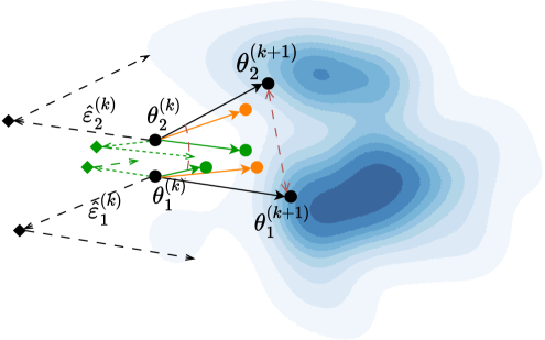
Interactive gradient directions and Connections to SAM. To gain further insight into the mechanism of FHBI and its underlying connections to SAM, consider the term in the descending step, which is related to .
The perturbed loss can be approximated as:
where involves the average . Consequently, the gradient of this perturbed loss indicates a direction that simultaneously minimizes - which approximates the sharpness of the th particle, as discussed by Foret et al. (2021) - and for all , which reflects the angular similarity in the directions of the two particles. Thus, in addition to minimizing the sharpness of each particle, the first term of the descent step acts as an angular repulsive force, promoting more diverse traveling directions for the particles. Besides, as discussed by Liu & Wang (2016b), the second term acts as a spatial repulsive force, driving the particles apart to prevent them from collapsing into a single mode. Consequently, FHBI is not merely an extension of SAM to multiple independent particles; it enables the sharpness and gradient directions of the particles to interact with one another. This insight about the mechanism underlying our algorithm is summarized in Figure 1. In Section 6, we empirically demonstrate that, compared to SVGD, FHBI not only effectively minimizes particle-wise sharpness and loss values but also fosters greater diversity in the travel directions of the particles during training. This increased directional diversity, combined with the kernel gradient term, further mitigates the risk of particles collapsing into a single mode and improve the final performance as presented in Section 5.
5 Experiments
| Natural | Specialized | Structured | ||||||||||||||||||
| Method |
CIFAR100 |
Caltech101 |
DTD |
Flower102 |
Pets |
SVHN |
Sun397 |
Camelyon |
EuroSAT |
Resisc45 |
Retinopathy |
Clevr-Count |
Clevr-Dist |
DMLab |
KITTI |
dSpr-Loc |
dSpr-Ori |
sNORB-Azim |
sNORB-Ele |
AVG |
| FFT | 68.9 | 87.7 | 64.3 | 97.2 | 86.9 | 87.4 | 38.8 | 79.7 | 95.7 | 84.2 | 73.9 | 56.3 | 58.6 | 41.7 | 65.5 | 57.5 | 46.7 | 25.7 | 29.1 | 65.6 |
| AdamW | 67.1 | 90.7 | 68.9 | 98.1 | 90.1 | 84.5 | 54.2 | 84.1 | 94.9 | 84.4 | 73.6 | 82.9 | 69.2 | 49.8 | 78.5 | 47.1 | 31.0 | 72.0 | ||
| SAM | 72.7 | 90.3 | 71.4 | 99.0 | 90.2 | 84.4 | 52.4 | 82.0 | 92.6 | 84.1 | 74.0 | 76.7 | 68.3 | 47.9 | 74.3 | 71.6 | 43.4 | 26.9 | 39.1 | 70.5 |
| DeepEns | 69.1 | 88.9 | 67.7 | 98.9 | 90.7 | 85.1 | 54.5 | 82.6 | 94.8 | 82.7 | 75.3 | 46.6 | 47.1 | 47.4 | 68.2 | 71.1 | 36.6 | 30.1 | 35.6 | 67.0 |
| BayesTune | 67.2 | 91.7 | 69.5 | 99.0 | 90.7 | 86.4 | 54.7 | 84.9 | 95.3 | 84.1 | 75.1 | 82.8 | 68.9 | 49.7 | 79.3 | 74.3 | 46.6 | 30.3 | 42.8 | 72.2 |
| SGLD | 68.7 | 91.0 | 67.0 | 98.6 | 89.3 | 83.0 | 51.6 | 81.2 | 93.7 | 83.2 | 76.4 | 80.0 | 70.1 | 48.2 | 76.2 | 71.1 | 39.3 | 31.2 | 38.4 | 70.4 |
| SVGD | 71.3 | 90.2 | 71.0 | 98.7 | 90.2 | 84.3 | 52.7 | 83.4 | 93.2 | 86.7 | 75.1 | 75.8 | 70.7 | 49.6 | 79.9 | 69.1 | 41.2 | 30.6 | 33.1 | 70.9 |
| 87.3 | 95.0 | 80.1 | 72.8 | 51.2 | 41.3 | |||||||||||||||
| FHBI | (.17) | (.42) | (.15) | (0.20) | (0.21) | (.52) | (.12) | (.31) | (.57) | (.21) | (.20) | (.16) | (.27) | (.47) | (.31) | (.50) | (.32) | (.36) | (.59) | |
Applications to Model Fine-tuning.
Bayesian inference methods have promising applications in model finetuning. In standard finetuning scenarios, we are given a pre-trained model . The objective is to find the optimal parameters , where represents an additional module, often lightweight and small relative to the full model. Several parameter-efficient finetuning strategies have been developed, including LoRA (Hu et al., 2021), Adapter (Houlsby et al., 2019), and others. Our experiments focus on finetuning the ViT-B/16 architecture (Dosovitskiy et al., 2021), pre-trained with the ImageNet-21K dataset (Deng et al., 2009), where is defined by the LoRA framework. For the Bayesian approaches, we aim to learn LoRA particles to obtain model instances . The final output is then computed as the average of the outputs from all these model instances.
Experimental Details.
To assess the effectiveness of FHBI, we conduct experiments on the VTAB-1K benchmark (Zhai et al., 2020), a diverse and challenging image classification/prediction suite consisting of 19 datasets from various domains. VTAB-1K covers various tasks across different semantics and object categories. The datasets are organized into Natural, Specialized, and Structured domains. Each dataset includes 1,000 training examples, with an official 80/20 train-validation split. We compared FHBI against seven baselines with three deterministic finetuning strategies including full finetuning, AdamW, and SAM, and four Bayesian inference techniques including Bayesian Deep Ensembles (Lakshminarayanan et al., 2017), BayesTune (Kim & Hospedales, 2023), Stochastic Gradient Langevin Dynamics (SGLD) (Welling & Teh, 2011), and Stein Variational Gradient Descent (SVGD) (Liu & Wang, 2016b).
We used ten warm-up epochs, a batch size 64, and the cosine annealing learning rate scheduler for all settings. The experiments were run with PyTorch on a Tesla V100 GPU with 40GB of RAM. FHBI involves three hyperparameters: the learning rate , ascent step size , and kernel width . We tuned these hyperparameters using the provided validation set, where the candidate sets are formed as . Detailed chosen hyperparameters and data augmentations for each dataset are reported in Appendix B. For each experiment, we conducted five runs of FHBI and reported the mean and standard deviation. All methods except AdamW and full finetuning were trained with four particles on the same set of LoRA parameters.
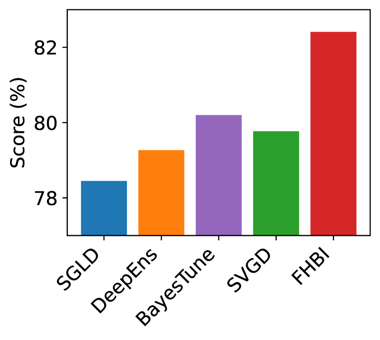
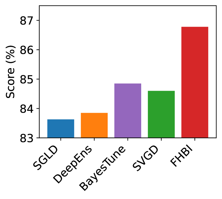
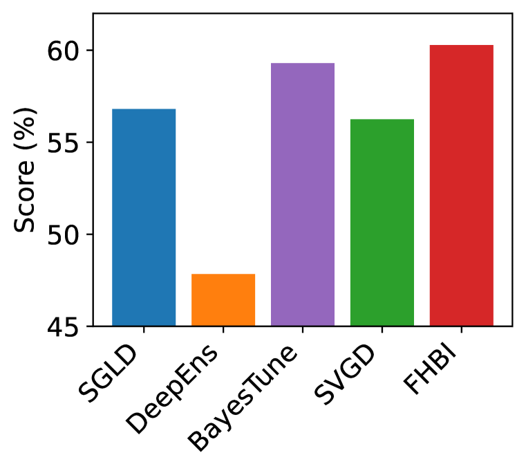
Experimental Results.
To evaluate the effectiveness of our method, we first present the classification accuracy results in Table LABEL:table:_accuracy. FHBI notably improves compared to the baselines, outperforming them in most settings. Compared to other particle sampling methods, including SGLD and SVGD, FHBI consistently performs better across all settings. Moreover, FHBI improves upon SAM by a margin of , highlighting the advantages of using multiple particles with the underlying interactive gradient directions as previously discussed in Section 4.1. Additionally, as illustrated in Figure 2, FHBI shows the highest performance across all three domains, further solidifying its advantage over the Bayesian inference baselines.
To further assess the robustness of FHBI, we evaluate the Expected Calibration Error (ECE) of each setting. This score measures the maximum discrepancy between the model’s accuracy and confidence. As indicated in Table LABEL:table:_ece, even though there is typically a trade-off between accuracy and ECE, our approach achieves a good balance between the ECE and the classification accuracy.
| Natural | Specialized | Structured | ||||||||||||||||||
| Method |
CIFAR100 |
Caltech101 |
DTD |
Flower102 |
Pets |
SVHN |
Sun397 |
Camelyon |
EuroSAT |
Resisc45 |
Retinopathy |
Clevr-Count |
Clevr-Dist |
DMLab |
KITTI |
dSpr-Loc |
dSpr-Ori |
sNORB-Azi |
sNORB-Ele |
AVG |
| FFT | 0.29 | 0.23 | 0.20 | 0.13 | 0.27 | 0.19 | 0.45 | 0.21 | 0.13 | 0.18 | 0.17 | 0.41 | 0.44 | 0.42 | 0.22 | 0.14 | 0.23 | 0.24 | 0.40 | 0.26 |
| AdamW | 0.38 | 0.19 | 0.18 | 0.05 | 0.09 | 0.10 | 0.14 | 0.11 | 0.09 | 0.12 | 0.11 | 0.12 | 0.19 | 0.34 | 0.18 | 0.14 | 0.21 | 0.18 | 0.31 | 0.17 |
| SAM | 0.21 | 0.25 | 0.20 | 0.11 | 0.12 | 0.15 | 0.14 | 0.17 | 0.16 | 0.14 | 0.09 | 0.12 | 0.17 | 0.24 | 0.16 | 0.21 | 0.19 | 0.13 | 0.16 | 0.16 |
| DeepEns | 0.24 | 0.12 | 0.22 | 0.04 | 0.10 | 0.13 | 0.23 | 0.16 | 0.07 | 0.15 | 0.21 | 0.31 | 0.32 | 0.36 | 0.32 | 0.31 | 0.16 | 0.29 | 0.20 | |
| BayesTune | 0.32 | 0.08 | 0.20 | 0.03 | 0.85 | 0.12 | 0.22 | 0.13 | 0.07 | 0.13 | 0.22 | 0.12 | 0.23 | 0.30 | 0.24 | 0.28 | 0.28 | 0.31 | 0.26 | 0.23 |
| SGLD | 0.26 | 0.20 | 0.17 | 0.05 | 0.18 | 0.14 | 0.23 | 0.18 | 0.09 | 0.12 | 0.32 | 0.26 | 0.29 | 0.21 | 0.26 | 0.42 | 0.39 | 0.24 | 0.22 | |
| SVGD | 0.20 | 0.13 | 0.19 | 0.04 | 0.16 | 0.09 | 0.20 | 0.15 | 0.11 | 0.13 | 0.12 | 0.17 | 0.21 | 0.30 | 0.18 | 0.21 | 0.25 | 0.14 | 0.26 | 0.18 |
| FHBI | 0.19 | 0.10 | 0.16 | 0.06 | 0.06 | 0.09 | 0.16 | 0.09 | 0.05 | 0.12 | 0.08 | 0.14 | 0.15 | 0.21 | 0.15 | 0.16 | 0.18 | 0.11 | 0.07 | |
6 Ablation Studies
6.1 Effect of #particles
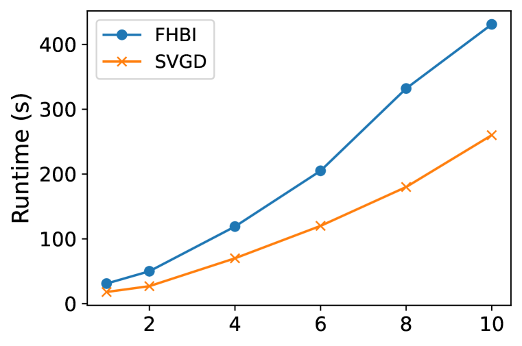
To understand the impact of varying the number of particles, we conducted experiments on the seven Natural datasets, reporting both accuracy and per-epoch runtime. We compared FHBI with SVGD and SAM. Figure 3 and Table 3 indicate that multiple particles result in significant performance improvements compared to a single particle. However, while increasing the number of particles enhances performance, it introduces a tradeoff regarding runtime and memory required to store the models. Based on these observations, we found that using provides an optimal balance between performance gains and computational overhead.
| #Particles |
CIFAR100 |
Caltech101 |
DTD |
Flower102 |
Pets |
SVHN |
Sun397 |
|---|---|---|---|---|---|---|---|
| 1p (SAM) | 72.7 | 90.3 | 71.4 | 99.0 | 90.2 | 84.4 | 52.4 |
| 4p | 74.8 | 93.0 | 74.3 | 99.4 | 92.4 | 87.5 | 56.5 |
| 10p | 75.0 | 93.2 | 75.0 | 99.1 | 92.4 | 87.9 | 58.3 |
6.2 Particles Sharpness and Gradient Diversity
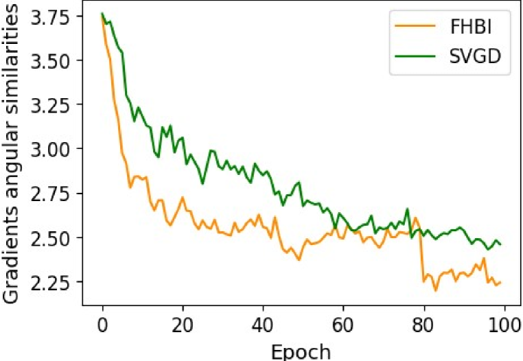
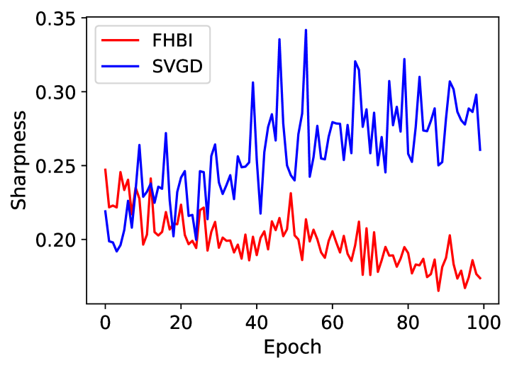
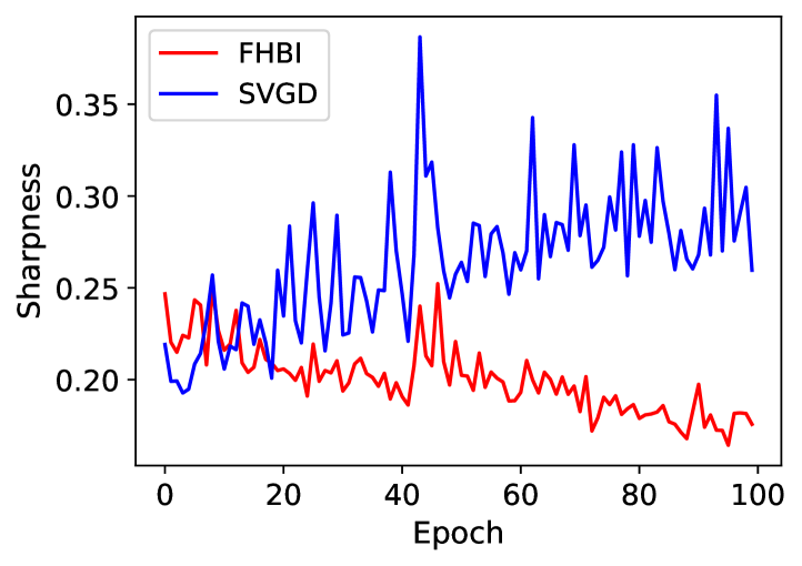
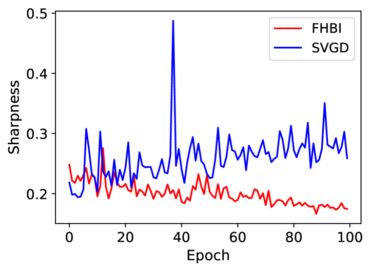
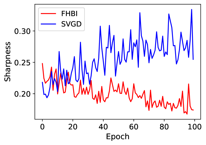
As discussed in Section 4.1 and Section 5, FHBI shares implicit connections with SAM by minimizing particle-wise sharpness and diversifying particle travel directions, improving the final performance. To empirically verify this hypothesis about the behavior of our algorithm, we contrast FHBI with SVGD on the KITTI dataset. Four particles are initialized at the same location. We measured: 1) the evolution of sharpness of each particle, defined as according to Foret et al. (2021), and 2) the evolution of gradients angular diversity, quantified as the Frobenius norm of the covariance matrix formed by the particle gradients. As shown in Figure 5, FHBI not only results in significantly lower and more stable sharpness evolution but also encourages less congruent gradient directions, promoting particles to explore diverse trajectories. Hence, FHBI effectively reduces particle sharpness while promoting angular diversity, improves generalization ability and avoids overfitting by collapsing into a single mode.
7 Conclusion
We introduce Flat Hilbert Bayesian Inference (FHBI), a particle-sampling method designed to enhance generalization ability beyond previous Bayesian inference approaches. This algorithm is based on a theoretical framework that extends generalization principles from Euclidean spaces to the infinite-dimensional RKHS. In our experiments on the VTAB-1K benchmark, FHBI consistently demonstrated performance improvements over six baseline methods by notable margins.
Limitations and Future Directions.
Similar to other particle-sampling methods, FHBI needs to store multiple models. Although it remains well-suited for fine-tuning since the additional modules are typically lightweight, this requirement is a memory bottleneck for larger models. Given that the variational inference (VI) approaches can alleviate this issue, an avenue for future research is to extend the concept of sharpness over functional spaces introduced by our theorems to the VI techniques to improve the generalization ability of these methods without storing multiple models.
Reproducibility Statement
We open-source our implementation and provide the configs and log files at https://anonymous.4open.science/r/Flat-Hilbert-Variational-Inference-008F/
References
- Abbas et al. (2022) Momin Abbas, Quan Xiao, Lisha Chen, Pin-Yu Chen, and Tianyi Chen. Sharp-maml: Sharpness-aware model-agnostic meta learning. arXiv preprint arXiv:2206.03996, 2022.
- Aronszajn (1950) Nachman Aronszajn. Theory of reproducing kernels. Transactions of the American Mathematical Society, 68(3):337–404, 1950.
- Bahri et al. (2022) Dara Bahri, Hossein Mobahi, and Yi Tay. Sharpness-aware minimization improves language model generalization. In Proceedings of the 60th Annual Meeting of the Association for Computational Linguistics (Volume 1: Long Papers), pp. 7360–7371, Dublin, Ireland, May 2022. Association for Computational Linguistics. doi: 10.18653/v1/2022.acl-long.508. URL https://aclanthology.org/2022.acl-long.508.
- Blundell et al. (2015) Charles Blundell, Julien Cornebise, Koray Kavukcuoglu, and Daan Wierstra. Weight uncertainty in neural network. In International conference on machine learning, pp. 1613–1622. PMLR, 2015.
- Caldarola et al. (2022) Debora Caldarola, Barbara Caputo, and Marco Ciccone. Improving generalization in federated learning by seeking flat minima. In European Conference on Computer Vision, pp. 654–672. Springer, 2022.
- Cha et al. (2021) Junbum Cha, Sanghyuk Chun, Kyungjae Lee, Han-Cheol Cho, Seunghyun Park, Yunsung Lee, and Sungrae Park. Swad: Domain generalization by seeking flat minima. Advances in Neural Information Processing Systems, 34:22405–22418, 2021.
- Chaudhari et al. (2017) Pratik Chaudhari, Anna Choromańska, Stefano Soatto, Yann LeCun, Carlo Baldassi, Christian Borgs, Jennifer T. Chayes, Levent Sagun, and Riccardo Zecchina. Entropy-sgd: biasing gradient descent into wide valleys. Journal of Statistical Mechanics: Theory and Experiment, 2019, 2017.
- Chen et al. (2014) Tianqi Chen, Emily Fox, and Carlos Guestrin. Stochastic gradient Hamiltonian Monte Carlo. In International conference on machine learning, pp. 1683–1691. PMLR, 2014.
- Chen et al. (2021) Xiangning Chen, Cho-Jui Hsieh, and Boqing Gong. When vision transformers outperform resnets without pre-training or strong data augmentations. arXiv preprint arXiv:2106.01548, 2021.
- Deng et al. (2009) Jia Deng, Wei Dong, Richard Socher, Li-Jia Li, Kai Li, and Li Fei-Fei. Imagenet: A large-scale hierarchical image database. In 2009 IEEE Conference on Computer Vision and Pattern Recognition, pp. 248–255, 2009. doi: 10.1109/CVPR.2009.5206848.
- Dinh et al. (2017) Laurent Dinh, Razvan Pascanu, Samy Bengio, and Yoshua Bengio. Sharp minima can generalize for deep nets. In International Conference on Machine Learning, pp. 1019–1028. PMLR, 2017.
- Dosovitskiy et al. (2021) Alexey Dosovitskiy, Lucas Beyer, Alexander Kolesnikov, Dirk Weissenborn, Xiaohua Zhai, Thomas Unterthiner, Mostafa Dehghani, Matthias Minderer, Georg Heigold, Sylvain Gelly, Jakob Uszkoreit, and Neil Houlsby. An image is worth 16x16 words: Transformers for image recognition at scale, 2021. URL https://arxiv.org/abs/2010.11929.
- Dusenberry et al. (2020) Michael Dusenberry, Ghassen Jerfel, Yeming Wen, Yian Ma, Jasper Snoek, Katherine Heller, Balaji Lakshminarayanan, and Dustin Tran. Efficient and scalable Bayesian neural nets with rank-1 factors. In International conference on machine learning, pp. 2782–2792. PMLR, 2020.
- Dziugaite & Roy (2017) Gintare Karolina Dziugaite and Daniel M. Roy. Computing nonvacuous generalization bounds for deep (stochastic) neural networks with many more parameters than training data. In UAI. AUAI Press, 2017.
- Foret et al. (2021) Pierre Foret, Ariel Kleiner, Hossein Mobahi, and Behnam Neyshabur. Sharpness-aware minimization for efficiently improving generalization. In 9th International Conference on Learning Representations, ICLR 2021, Virtual Event, Austria, May 3-7, 2021. OpenReview.net, 2021. URL https://openreview.net/forum?id=6Tm1mposlrM.
- Fort & Ganguli (2019) Stanislav Fort and Surya Ganguli. Emergent properties of the local geometry of neural loss landscapes. arXiv preprint arXiv:1910.05929, 2019.
- Ghosh et al. (2018) Soumya Ghosh, Jiayu Yao, and Finale Doshi-Velez. Structured variational learning of Bayesian neural networks with horseshoe priors. In International Conference on Machine Learning, pp. 1744–1753. PMLR, 2018.
- Graves (2011) Alex Graves. Practical variational inference for neural networks. Advances in Neural Information Processing Systems, 24, 2011.
- Gupta & Nagar (2018) Arjun K Gupta and Daya K Nagar. Matrix variate distributions. Chapman and Hall/CRC, 2018.
- Hochreiter & Schmidhuber (1994) Sepp Hochreiter and Jürgen Schmidhuber. Simplifying neural nets by discovering flat minima. In NIPS, pp. 529–536. MIT Press, 1994.
- Houlsby et al. (2019) Neil Houlsby, Andrei Giurgiu, Stanislaw Jastrzebski, Bruna Morrone, Quentin de Laroussilhe, Andrea Gesmundo, Mona Attariyan, and Sylvain Gelly. Parameter-efficient transfer learning for nlp, 2019. URL https://arxiv.org/abs/1902.00751.
- Hu et al. (2021) Edward J. Hu, Yelong Shen, Phillip Wallis, Zeyuan Allen-Zhu, Yuanzhi Li, Shean Wang, Lu Wang, and Weizhu Chen. Lora: Low-rank adaptation of large language models, 2021. URL https://arxiv.org/abs/2106.09685.
- Izmailov et al. (2018) Pavel Izmailov, Dmitrii Podoprikhin, Timur Garipov, Dmitry P. Vetrov, and Andrew Gordon Wilson. Averaging weights leads to wider optima and better generalization. In UAI, pp. 876–885. AUAI Press, 2018.
- Jiang et al. (2020) Yiding Jiang, Behnam Neyshabur, Hossein Mobahi, Dilip Krishnan, and Samy Bengio. Fantastic generalization measures and where to find them. In ICLR. OpenReview.net, 2020.
- Kaddour et al. (2022) Jean Kaddour, Linqing Liu, Ricardo Silva, and Matt J. Kusner. Questions for flat-minima optimization of modern neural networks. CoRR, abs/2202.00661, 2022. URL https://arxiv.org/abs/2202.00661.
- Keskar et al. (2016) Nitish Shirish Keskar, Dheevatsa Mudigere, Jorge Nocedal, Mikhail Smelyanskiy, and Ping Tak Peter Tang. On large-batch training for deep learning: Generalization gap and sharp minima. CoRR, abs/1609.04836, 2016. URL http://arxiv.org/abs/1609.04836.
- Keskar et al. (2017) Nitish Shirish Keskar, Dheevatsa Mudigere, Jorge Nocedal, Mikhail Smelyanskiy, and Ping Tak Peter Tang. On large-batch training for deep learning: Generalization gap and sharp minima. In ICLR. OpenReview.net, 2017.
- Kim & Hospedales (2023) Minyoung Kim and Timothy M Hospedales. Bayestune: Bayesian sparse deep model fine-tuning. In Advances in Neural Information Processing Systems 36 (NeurIPS 2023), volume 36, pp. 65317–65365. Curran Associates Inc, December 2023. URL https://neurips.cc/Conferences/2023. Thirty-Seventh Conference on Neural Information Processing Systems, NeurIPS 2023 ; Conference date: 10-12-2023 Through 16-12-2023.
- Kim et al. (2022) Minyoung Kim, Da Li, Shell Xu Hu, and Timothy M. Hospedales. Fisher SAM: Information geometry and sharpness aware minimisation, 2022. URL https://arxiv.org/abs/2206.04920.
- Kingma & Welling (2013) Diederik P Kingma and Max Welling. Auto-encoding variational Bayes. arXiv preprint arXiv:1312.6114, 2013.
- Kingma et al. (2015) Durk P Kingma, Tim Salimans, and Max Welling. Variational dropout and the local reparameterization trick. Advances in Neural Information Processing Systems, 28, 2015.
- Kreyszig (1978) Erwin Kreyszig. Introductory Functional Analysis with Applications. John Wiley & Sons, 1978.
- Lakshminarayanan et al. (2017) Balaji Lakshminarayanan, Alexander Pritzel, and Charles Blundell. Simple and scalable predictive uncertainty estimation using deep ensembles, 2017. URL https://arxiv.org/abs/1612.01474.
- Li et al. (2022) Zhouzi Li, Zixuan Wang, and Jian Li. Analyzing sharpness along gd trajectory: Progressive sharpening and edge of stability, 2022.
- Liu & Wang (2016a) Qiang Liu and Dilin Wang. Stein variational gradient descent: A general purpose Bayesian inference algorithm. Advances in Neural Information Processing Systems, 29, 2016a.
- Liu & Wang (2016b) Qiang Liu and Dilin Wang. Stein variational gradient descent: A general purpose Bayesian inference algorithm. In D. Lee, M. Sugiyama, U. Luxburg, I. Guyon, and R. Garnett (eds.), Advances in Neural Information Processing Systems, volume 29. Curran Associates, Inc., 2016b. URL https://proceedings.neurips.cc/paper_files/paper/2016/file/b3ba8f1bee1238a2f37603d90b58898d-Paper.pdf.
- Louizos & Welling (2017) Christos Louizos and Max Welling. Multiplicative normalizing flows for variational Bayesian neural networks. In International Conference on Machine Learning, pp. 2218–2227. PMLR, 2017.
- Möllenhoff & Khan (2023) Thomas Möllenhoff and Mohammad Emtiyaz Khan. SAM as an optimal relaxation of bayes. In The Eleventh International Conference on Learning Representations, 2023. URL https://openreview.net/forum?id=k4fevFqSQcX.
- Neal (1996) Radford M. Neal. Bayesian Learning for Neural Networks. Springer-Verlag, Berlin, Heidelberg, 1996. ISBN 0387947248.
- Neyshabur et al. (2017) Behnam Neyshabur, Srinadh Bhojanapalli, David McAllester, and Nati Srebro. Exploring generalization in deep learning. Advances in Neural Information Processing Systems, 30, 2017.
- Nguyen et al. (2023) Van-Anh Nguyen, Tung-Long Vuong, Hoang Phan, Thanh-Toan Do, Dinh Phung, and Trung Le. Flat seeking bayesian neural networks. Advances in Neural Information Processing Systems, 2023.
- Pereyra et al. (2017) Gabriel Pereyra, George Tucker, Jan Chorowski, Lukasz Kaiser, and Geoffrey E. Hinton. Regularizing neural networks by penalizing confident output distributions. In ICLR (Workshop). OpenReview.net, 2017.
- Petzka et al. (2021) Henning Petzka, Michael Kamp, Linara Adilova, Cristian Sminchisescu, and Mario Boley. Relative flatness and generalization. In NeurIPS, pp. 18420–18432, 2021.
- Qu et al. (2022) Zhe Qu, Xingyu Li, Rui Duan, Yao Liu, Bo Tang, and Zhuo Lu. Generalized federated learning via sharpness aware minimization. arXiv preprint arXiv:2206.02618, 2022.
- Ritter et al. (2018) Hippolyt Ritter, Aleksandar Botev, and David Barber. A scalable laplace approximation for neural networks. In 6th International Conference on Learning Representations, ICLR 2018-Conference Track Proceedings, volume 6. International Conference on Representation Learning, 2018.
- Rossi et al. (2020) Simone Rossi, Sebastien Marmin, and Maurizio Filippone. Walsh-Hadamard variational inference for Bayesian deep learning. Advances in Neural Information Processing Systems, 33:9674–9686, 2020.
- Wang et al. (2023) Pengfei Wang, Zhaoxiang Zhang, Zhen Lei, and Lei Zhang. Sharpness-aware gradient matching for domain generalization. In Proceedings of the IEEE/CVF Conference on Computer Vision and Pattern Recognition, pp. 3769–3778, 2023.
- Welling & Teh (2011) Max Welling and Yee Whye Teh. Bayesian learning via stochastic gradient Langevin dynamics. In Proceedings of the 28th International Conference on International Conference on Machine Learning, ICML’11, pp. 681–688, Madison, WI, USA, 2011. Omnipress. ISBN 9781450306195.
- Zhai et al. (2020) Xiaohua Zhai, Joan Puigcerver, Alexander Kolesnikov, Pierre Ruyssen, Carlos Riquelme, Mario Lucic, Josip Djolonga, Andre Susano Pinto, Maxim Neumann, Alexey Dosovitskiy, Lucas Beyer, Olivier Bachem, Michael Tschannen, Marcin Michalski, Olivier Bousquet, Sylvain Gelly, and Neil Houlsby. A large-scale study of representation learning with the visual task adaptation benchmark, 2020. URL https://arxiv.org/abs/1910.04867.
- Zhang et al. (2018) Guodong Zhang, Shengyang Sun, David Duvenaud, and Roger Grosse. Noisy natural gradient as variational inference. In International Conference on Machine Learning, pp. 5852–5861. PMLR, 2018.
- Zhang et al. (2023) Xingxuan Zhang, Renzhe Xu, Han Yu, Yancheng Dong, Pengfei Tian, and Peng Cui. Flatness-aware minimization for domain generalization. In Proceedings of the IEEE/CVF International Conference on Computer Vision, pp. 5189–5202, 2023.
- Zhou et al. (2024) Tian-Yi Zhou, Namjoon Suh, Guang Cheng, and Xiaoming Huo. Approximation of RKHS functionals by neural networks, 2024. URL https://arxiv.org/abs/2403.12187.
Supplement to “Improving generalization with Flat Hilbert Variational Inference”
Appendix A Missing proofs
We introduce a few additional notations for the sake of the missing proofs of the main theoretical results. Given a RKHS equipped with the inner product and the norm operator . We define the single-sample loss function on the functional space to be a map:
Define the general functional loss and the empirical functional loss . Throughout the proof, we assume that the parameter space is bounded by , and the data is al bounded that for some .
We introduce the following lemmas that will be used throughout the proof of our main theorems.
Lemma 2 (Approximation of RKHS functionals).
Let for some . Consider with induced by some Mercer kernel which is -Holder continuous for with constant . Suppose is Holder continuous for with constant . There exists some such that for every with , by taking some fixed with , we have a tanh neural network with two hidden layers of widths at most and parameters satisfying
| (11) |
with
where is the Gram matrix of .
Proof.
The proof can be found in Zhou et al. (2024) ∎
Lemma 3 (Product of RKHSs).
Given RKHSs , each defined on corresponding sets with kernels respectively. Then, is also an RKHS, with kernel that is the product of the individual kernels.
Proof.
The product space consists of tuples of functions . Firstly, we define the inner product in as:
This definition naturally defines a Hilbert space structure on since each is a Hilber space, and the sum of inner products is linear and positive definite. Now we define the kernel for the product space:
Notice that the pointwise product of positive definite kernels is a positive definite kernel, hence this kernel is valid.
We now verify the reproducing property of . Consider a function , and evaluate the function at a point .
The reproducing property in each individual RKHS implies that:
Hence, for the function , we get:
Thus, the reproducing property holds for the product space . Since is a Hilbert space and the kernel satisfies the reproducing property, we conclude that is another RKHS. ∎
A.1 Proof of Theorem 1
Theorem 3.
For any and any distribution , with probability over the choice of the training set ,
Proof.
is a functional that maps from to . Notice that is a RKHS, and for some are Euclidean spaces, which are also instances of RKHS. Moreover, the product of RKHS’s is also a RKHS according to Lemma 3. Hence, is also a RKHS. According to Lemma 2, there exists points , and a two-layer neural network parameterized by so that
for every . Consider so that , it implies . Denote for some , by invoking the inequality from Foret et al. (2021), let , it follows that:
By definition, a RKHS is a closed Hilbert space. Then, there exists a sequence so that that gets arbitrarily close to . Then, for any , it follows:
This is true for any . Hence, it implies
which concludes our proof. ∎
A.2 Proof of Theorem 2
Now we can prove the Theorem 2. We restate the theorem
Theorem 4.
For any target distribution , reference distribution , and any , we have the following bound between the general KL loss and the empirical KL loss
Proof.
Consider the left-hand side, we have:
On the other hand, we also have:
We define to be the functional such that:
According to Theorem 1, we have:
| (12) | ||||
| (13) |
Moreover, the model and data spaces are bounded, so and are bounded. Then, there exists constants such that , which also implies and . It follows that for all :
| (14) |
Appendix B Experimental Details
B.1 Chosen Hyperparameters
We grid-search hyperparameters on the validation set, where the key hyperparameters are: the kernel width , the initial learning rate , and the ascend step size . The candidate sets are formed as . The chosen hyperparameters are as follows : CIFAR100 = , Caltech101 = , DTD = , Flowers102 = , Pets = , SVHN = , Sun397 = , Patch-Camelyon = , DMLab = , EuroSAT = , Resisc45 = , Diabetic- Retinopathy = , Clevr-Count = , Clevr-Dist = , KITTI = , dSprites-loc = , dSprites-ori = , smallNorb-azi = , smallNorb-ele = .
B.2 Data Augmentations
Our implementation is based on the repository V-PETL. Similar to this repository, we use a different data augmentation among the following three augmentations for each dataset. In particular, the data augmentations that we used for each setting are:
-
•
For CIFAR100, DTD, Flower102, Pets, Sun397
self.transforms_train = transforms.Compose([transforms.RandomResizedCrop((self.size, self.size),scale=(self.min_scale, self.max_scale),),transforms.RandomHorizontalFlip(self.flip_prob),transforms.TrivialAugmentWide()if self.use_trivial_augelse transforms.RandAugment(self.rand_aug_n,self.rand_aug_m),transforms.ToTensor(),transforms.Normalize(mean=[0.485, 0.456, 0.406],std=[0.229, 0.224, 0.225])]),transforms.RandomErasing(p=self.erase_prob),])self.transforms_test = transforms.Compose([transforms.Resize((self.size, self.size),),transforms.ToTensor(),transforms.Normalize(mean=[0.485, 0.456, 0.406],std=[0.229, 0.224, 0.225])]),]) -
•
For Caltech101, Clevr-Dist, Dsprites-Loc, Dsprites-Ori, SmallNorb-Azi, SmallNorb-Ele:
self.transform_train = transforms.Compose([transforms.Resize((224, 224)),transforms.ToTensor(),transforms.Normalize(mean=[0.485, 0.456, 0.406],std=[0.229, 0.224, 0.225])])self.transform_test = transforms.Compose([transforms.Resize((224, 224)),transforms.ToTensor(),transforms.Normalize(mean=[0.485, 0.456, 0.406],std=[0.229, 0.224, 0.225])]) -
•
For Clevr-Count, DMLab, EuroSAT, KITTI, Patch Camelyon, Resisc45, SVHN, Diabetic Retinopathy:
from timm.data import create_transformself.transform_train = create_transform(input_size=(224, 224),is_training=True,color_jitter=0.4,auto_augment=’rand-m9-mstd0.5-inc1’,re_prob=0.0,re_mode=’pixel’,re_count=1,interpolation=’bicubic’,)aug_transform.transforms[0] = transforms.Resize((224, 224),interpolation=3)self.transform_test = transforms.Compose([transforms.Resize((224, 224)),transforms.ToTensor(),transforms.Normalize(mean=[0.485, 0.456, 0.406],std=[0.229, 0.224, 0.225])])