Adaptive Control of multirotor in Continuous Time

Single-shot Learning of a multirotor Controller

Transfer Learning of a Multirotor Control System

Learning a Multirotor Control System via Transfer Learning

Multirotor Controller Training using Transfer Learning

Multirotor Controller Single-shot Training in a Transfer Learning Framework
based on Retrospective Cost Optimization

Sim-to-Real Multirotor Controller Learning
based on Single-shot Retrospective Cost Optimization

Sim-to-Real Multirotor Controller Single-shot Learning

Abstract

This paper demonstrates the sim-to-real capabilities of retrospective cost optimization-based adaptive control for multirotor stabilization and trajectory-tracking problems. First, a continuous-time version of the widely used discrete-time retrospective control adaptive control algorithm is developed. Next, a computationally inexpensive 12-degree-of-freedom model of a multirotor is used to learn the control system in a simulation environment with a single trajectory. Finally, the performance of the learned controller is verified in a complex and realistic multirotor model in simulation and with a physical quadcopter in a waypoint command and a helical trajectory command.

keywords: Aerial Robotics, Learning and Adaptive Systems, Optimization and Optimal Control, Quadrotor UAV.

I Introduction

Multirotor unmanned aerial vehicles are being increasingly used in various sectors due to their simple structure and vertical take-off and landing capabilities. Applications now include a wide variety, such as agricultural applications [1] and search and rescue missions [2]. Despite multirotors’ successes, commercial flight controllers and autopilots are only well-tuned for well-established airframes. Due to underactuated nonlinear dynamics, parasitic vibrational effects, and fluid-structure interactions, which are extremely difficult to model, model-based control design for multirotors is impractical. The uncertainty and time-varying nature of the physical parameters make this approach increasingly difficult. Furthermore, changes in the payload or physical modifications due to component upgrades degrade the nominal controller performance.

Learning-based, data-driven, and adaptive control techniques are thus ideally suited to design control system for multirotor systems since such techniques can compensate for unknown, unmodeled, and uncertain dynamics. Several learning-based techniques have been explored for controller design. In particular, reinforcement learning has been explored in [3, 4, 5, 6, 7, 8, 9, 10] to design multirotor controllers. However, these approaches require an existing stabilizing controller to improve it and several iterations of the experiment to generate sufficiently rich data to learn the controller. A nature-inspired evolutionary optimization algorithm is used for tuning PID controllers in [11], where the integral of squared error is used as the fitness function and minimized over generations in the context of evolutionary optimization. However, as the authors note, the position and attitude controllers are separately tuned and require one of them to be well tuned to tune the other. Auto differentiation for gradient-based optimization is explored in [12], however, this approach requires a sufficiently realistic model of the system.

In contrast, the current work uses retrospective cost optimization, which does not require a prior stabilizing controller and optimizes the controller in a single experiment. Respective cost adaptive control (RCAC) is a discrete-time output feedback adaptive control technique that is applicable to stabilization, command-following, and disturbance rejection problems. The RCAC algorithm, its connection to linear quadratic control, and its extension to adaptive PID control are described in detail in [13, 14]. The discrete-time RCAC technique has been successfully applied to learn multirotor controllers [15, 16]. However, the discrete-time control design is vulnerable to the sampling time. Furthermore, the learned controller does not have a direct interpretation in terms of stability and transient performance. A key contribution of this work is thus the development and application of a continuous-time retrospective cost adaptive control (CT-RCAC) to learn the multirotor controller.

The main contribution of this work is the demonstration of the sim-to-real transfer learning capability of the CT-RCAC algorithm in the context of learning a multirotor controller. Sim-to-real transfer learning is a subcategory of homogeneous transfer learning [17]. In this framework, the model is trained in a simulation environment, a source of learning, and then deployed on a physical robot or system in a real environment, a target of learning. The key requirement of the sim-to-real transfer learning is thus sufficient similarity in the feature space, such as position, velocity states, and underlying dynamics.

The paper is organized as follows. Section II briefly reviews the multirotor dynamics and the control system architecture used in this work, Section III presents the continuous-time retrospective cost adaptive control algorithm, and Section IV describes applying the transfer learning framework to train the multirotor controller in a computationally inexpensive simulation for a physical quadcopter. The paper concludes with a summary in Section V.

II Multirotor Dynamics and Control

This section briefly reviews the multirotor dynamics and the classical inner-outer control architecture. A detailed derivation of the multirotor dynamics is given in [18, 15].

II-A Multirotor Dynamics

A multirotor can be modeled as a rigid body with a force applied along a body-fixed axis and a torque applied to the rigid body. The translational dynamics of a multirotor is

$$m\ddot{r}=mge_{3}+{\mathcal{O}}e_{3}f,$$ (1)

where $m$ is the mass of the multirotor, $r\in{\mathbb{R}}^{3}$ is the position of multirotor relative to a fixed point in an inertial frame, $g$ is the acceleration due to gravity, $e_{3}\in{\mathbb{R}}^{3}$ is the third column of the $3\times 3$ identity matrix, $f\in{\mathbb{R}}$ is the force applied along a body-fixed axis, and the orthonormal matrix ${\mathcal{O}}\in{\mathbb{R}}^{3\times 3}$ parameterizes the multirotor’s attitude relative to an inertial frame.

The rotational dynamics of a multirotor is

$$\dot{\mathcal{O}}=-\omega^{\times}{\mathcal{O}},$$ (2)

$$J\dot{\omega}+\omega\times J\omega=\tau,$$ (3)

where $\omega\in{\mathbb{R}}^{3}$ is the angular velocity vector of the multirotor relative to an inertial frame resolved in the body-fixed frame, $J\in{\mathbb{R}}^{3\times 3}$ is the moment of inertia matrix, and $\tau\in{\mathbb{R}}^{3}$ is the torque applied to the multirotor in the body-fixed frame.

Note that (1) models the translational motion of the multirotor, whereas (2), (3) model the rotational motion of the multirotor. This separation of translational and rotational motions facilitates the implementation of outer and inner loop architectures for trajectory tracking. However, note that the translational motion and the rotational motion of the multirotor are coupled via the attitude ${\mathcal{O}}$ in (1), and thus the outer and inner loop design cannot be entirely decoupled. In fact, it is precisely the coupling due to the ${\mathcal{O}}$ matrix which allows stabilization of the underactuated translational dynamics.

II-B Multirotor Control

This work considers a cascaded control system, as shown in Figure 1. The cascaded loop architecture is motivated by the time separation principle. The outer loop is designed to track the position references, whereas the inner loop is designed to track the attitude references. The cascaded loop architecture assumes that the inner loop dynamics are significantly faster than the outer loop dynamics. In this case, the three-dimensional force vector required to move the multirotor in a desired direction can be realized by adjusting the attitude of the multirotor so that the axis of the multirotor is along the direction of the force vector and modulating the total force exerted by the propellers.

Figure 1: Cascaded loop control architecture for a multirotor.

Since the inner loop, which regulates the rotational motion, is assumed to be significantly faster than the outer loop, the translational motion of the multirotor satisfies

$$m\ddot{r}_{1} =f_{r_{1}},$$ (4)

$$m\ddot{r}_{2} =f_{r_{2}},$$ (5)

$$m\ddot{r}_{3} =mg+f_{r_{3}},$$ (6)

where $r_{1},r_{2},$ and $r_{3}$ are the components of $r,$ $f_{r_{1}}$ and $f_{r_{2}}$ are the horizontal forces and $f_{r_{3}}$ is the vertical force on the multirotor. Note that (4)-(6) are linear and decoupled, where the effective forces $f_{r_{1}},f_{r_{2}}$ and $f_{r_{3}}$ are assumed to be realizable due to the faster rotational dynamics. The objective of the outer loop is thus to compute the force input to track a desired position reference, as shown in Figure 2. The position controller considered in this work consists of three decoupled controllers, each tasked to follow the corresponding position command.

Figure 2: Outer loop to track position reference.

The inner loop computes the moment required to realize the force vector desired by the outer loop by orienting the multirotor so that its force axis aligns with the desired force vector required by the outer loop. The computation of the desired attitude is described in detail in [15]. In terms of the 3-2-1 Euler angles, representing the yaw, roll, and pitch, (2) is

$$\dot{\Theta}=S(\Theta)\omega,$$ (7)

where $\Theta\in{\mathbb{R}}^{3}$ contains the three Euler angles. Note that the rotational motion of the multirotor is governed by the nonlinear coupled dynamics (7), (3). However, it is well known that for small Euler angles, the rotational dynamics consists of three decoupled double integrators similar to (4)-(6). Figure 3 shows the inner loop to track the desired attitude reference. The attitude controller considered in this work consists of three decoupled controllers, each tasked to follow the corresponding angle command.

Figure 3: Inner loop to track attitude reference.

To follow the position and angle references in the outer and the inner loop, we consider a modified cascaded P-PI architecture shown in Figure 4. As shown in Figure 4, the control $u$ is given by

$$u=k_{{\rm p},1}e+k_{{\rm p},2}e_{v}+k_{{\rm i}}\int e_{v},$$ (8)

where the tracking error $e\stackrel{{\scriptstyle\triangle}}{{=}}r-y$, $k_{{\rm p},1}$ and $k_{{\rm p},2}$ are the proportional gains, $k_{{\rm i}}$ is the integral gain, and $e_{v}\stackrel{{\scriptstyle\triangle}}{{=}}k_{{\rm p},1}e-\dot{y}.$ Note that the controller (8) can be written as

$$u(t)=\phi(t)\theta,$$ (9)

where the data regressor $\phi(t)\stackrel{{\scriptstyle\triangle}}{{=}}\begin{bmatrix}e&e_{v}&\int e_{v}\end{bmatrix}$ and the controller gain $\theta\stackrel{{\scriptstyle\triangle}}{{=}}\begin{bmatrix}k_{{\rm p},1}&k_{{\rm p},2}&k_{{\rm i}}\end{bmatrix}^{\rm T}.$ The controller gain $\theta$ is learned by retrospective cost optimize as described below.

Figure 4: Modified cascaded P-PI with control architecture for command following.

III Online Continuous Time Learning

This section describes the continuous-time retrospective cost adaptive control (CT-RCAC) used to optimize controller gains in this work.

Consider a dynamic system where $u(t)\in{\mathbb{R}}^{l_{u}}$ is the input, $y(t)\in{\mathbb{R}}^{l_{y}}$ is the measured output. The objective is to design an adaptive output feedback control law using only the measured $y(t)$ and the input $u(t)$ without using the underlying dynamics. Define the performance variable

$$z(t)\stackrel{{\scriptstyle\triangle}}{{=}}y(t)-r(t),$$ (10)

where $r(t)$ is the exogenous reference signal. The objective of the adaptive output feedback control law is thus to ensure that $z(t)\to 0.$

Consider a linearly parameterized control law

$$u(t)=\Phi(t)\theta(t),$$ (11)

where the regressor matrix $\Phi(t)\in{\mathbb{R}}^{l_{u}\times l_{\theta}}$ contains the measured data and the vector $\theta(t)\in{\mathbb{R}}^{l_{\theta}}$ contains the controller gains to be optimized. Various linear parameterizations of MIMO controllers are described in [19]. In this work, we use the SISO controller shown in (9).

Next, using (10), define the retrospective performance

$$\hat{z}(t) \stackrel{{\scriptstyle\triangle}}{{=}}z(t)+\Phi_{\rm f}(t)\hat{\theta}(t)-u_{\rm f}(t),$$ (12)

where $\hat{\theta}(t)$ is the controller gain to be optimized and the filtered regressor $\Phi_{\rm f}(t)$ and the filtered control $u_{\rm f}(t)$ are defined as

$$\Phi_{\rm f}(t) \stackrel{{\scriptstyle\triangle}}{{=}}G_{\rm f}(s)\left[\Phi(t)\right]\in{\mathbb{R}}^{l_{y}\times l_{\theta}},$$ (13)

$$u_{\rm f}(t) \stackrel{{\scriptstyle\triangle}}{{=}}G_{\rm f}(s)\left[u(t)\right]\in{\mathbb{R}}^{l_{y}\times l_{\theta}},$$ (14)

where $G_{\rm f}(s)$ is a dynamic filter.

Next, define the retrospective cost

$$J(t,\hat{\theta}) =\int_{0}^{t}\hat{z}(\tau)^{\rm T}R_{z}\hat{z}(\tau){\rm d}\tau+\hat{\theta}^{T}R_{\theta}\hat{\theta},$$ (15)

where $R_{z}$ and $R_{\theta}$ are positive definite weighting matrices of appropriate dimensions.

Proposition III.1.

Consider the cost function $J(t,\hat{\theta})$ given by (15). For all $t\geq 0,$ define the minimizer of $J(t,\hat{\theta})$ by

$$\theta^{*}(t)\stackrel{{\scriptstyle\triangle}}{{=}}\underset{\hat{\theta}\in{\mathbb{R}}^{l_{\theta}}}{\operatorname{argmin}}J(t,\hat{\theta}).$$ (16)

Then, for all $t\geq 0,$ the minimizer is given by

$$\theta^{*}(t)=P(t)b(t),$$ (17)

where

$$\dot{P}(t) =-P\Phi_{\rm f}^{\rm T}R_{z}\Phi_{\rm f}P,$$ (18)

$$\dot{b}(t) =2\Phi_{\rm f}^{\rm T}R_{z}(z-u_{\rm f}),$$ (19)

and $P(0)=R_{\theta}^{-1}$ and $b(0)=0.$

The proof of Proposition III.1 is omitted due to page restrictions.

Finally, for all $t\geq 0,$ the control is given by

$$u(t)=\Phi(t)\theta^{*}(t).$$ (20)

IV Transfer Learning

In this work, we use the 12dof model, described in Section II-A, as the source environment to learn the controller gains and a realistic Simulink model and the Holybro X500 V2 quadcopter as the target environment. In particular, we use the 12dof model, where $m=1.56$ $\rm kg$ and the inertia is $J={\rm diag}(0.03,0.03,0.05)$ $\rm kg\ m^{2}$ to learn the controller gains. These inertial properties are similar to the X500 Holybro quadcopter.

Recall that the control system consists of the outer and inner loops, as described in Section II-B. The outer loop consists of three decoupled P-PI controllers, shown in Figure 4, to track the three-dimensional position references, and the inner loop consists of three decoupled P-PI controllers to track the three-dimensional Euler angle references. Therefore, in total, 18 gains need to be learned. We use the CT-RCAC algorithm to learn the gains in a single trajectory, as discussed below.

Remark 1.

A 100-second simulation of the 12dof model takes approximately 3 seconds on an i7-13700HX Intel processor with 16 GB RAM, and thus the RCAC hyperparameters $G_{\rm f}(s),$ $R_{z},$ and $P_{0}$ are tuned by a trivial grid-search method. The tuned RCAC hyperparameters used to learn the controller gains are given in Table I.

Hyperparameters	$G_{\rm f}(s)$	$R_{z}$	$P(0)$
Outer loop $(r_{1},r_{2})$	$\dfrac{1}{s+0.5}$	$10^{4}$	$10^{3}$
Outer loop $(r_{3})$	$\dfrac{1}{(s+1.5)(s+3)}$	$10^{4}$	$10^{5}$
Inner loop	$\dfrac{1}{s+2}$	$10^{4}$	$10^{3}$

TABLE I: RCAC hyperparameters tuned with the 12 dof model in MATLAB.

First, we consider a waypoint command, where the quadcopter is commanded to fly from an initial point to a final point. Note that a velocity command is not specified. In this work, we set the initial point to $(0,0,0)$ and the final point to $(1,1,1).$ Thus, the position command is, for all $t\geq 0,$ $r_{{\rm d}1}=r_{{\rm d}2}=r_{{\rm d}3}=1.$ Figure 5 shows the a) position response, b) Euler angles response, c) the magnitude of the force and d) torque applied to the multirotor, respectively, e) controller gains in the outer loop, and f) controller gains in the inner loop. The RCAC hyperparameters used in this case are shown in Table I. Note that all controller gains are initialized at zero.

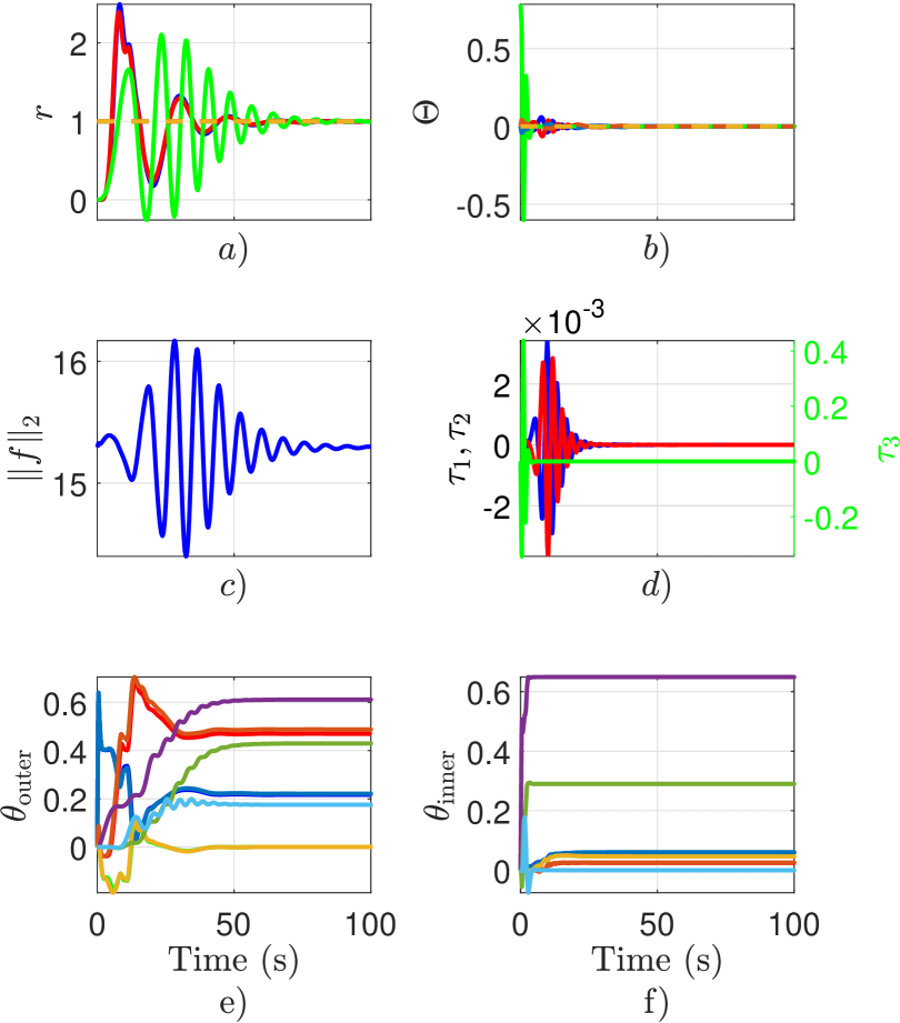
Figure 5: Learning with a waypoint command. a) position response, b) Euler angles response, c) the magnitude of the force and d) torque applied to the multirotor, respectively, e) controller gains in the outer loop, and f) controller gains in the inner loop.

Next, we consider a helical trajectory command, where the multirotor is commanded to follow a trajectory given by $r_{{\rm d}1}=\cos(\omega t),r_{{\rm d}2}=\sin(\omega t),$ and $r_{{\rm d}3}=\omega t.$ In this work, we set $\omega=0.1.$ Note that a velocity command is embedded in the position command. Figure 6 shows the a) position response, b) Euler angles response, c) the magnitude of the force and d) torque applied to the multirotor, respectively, e) controller gains in the outer loop, and f) controller gains in the inner loop. Note that the RCAC hyperparameters are not re-tuned. Furthermore, to emphasize that no prior stabilizing controller is needed, all controller gains are initialized at zero. Figure 7 shows the trajectory-tracking response to the helical trajectory command with the learning controller. Note that the tracking performance improves the longer the simulation runs.

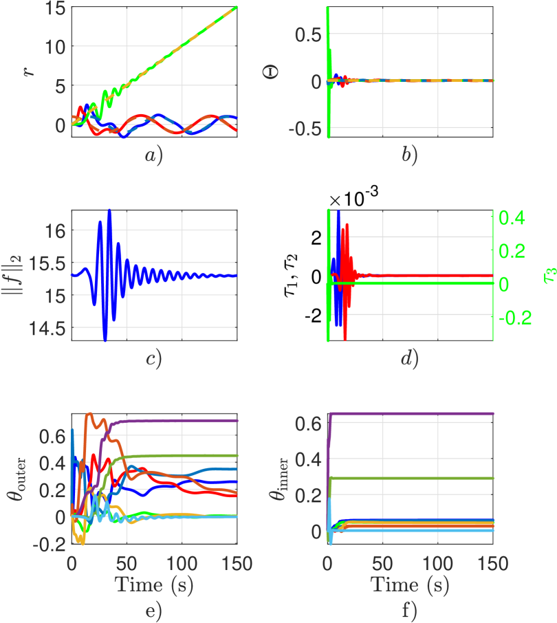
Figure 6: Learning with a helical trajectory command. a) position response, b) Euler angles response, c) the magnitude of the force and d) torque applied to the multirotor, respectively, e) controller gains in the outer loop, and f) controller gains in the inner loop.

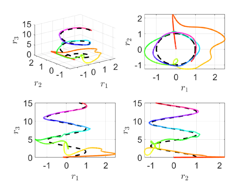
Figure 7: Trajectory-tracking response to the helical trajectory command with the learning controller.

The controller gains learned with the waypoint and the helical trajectory commands are shown in Table II.

Loop	Controller gains with waypoint command
Outer	$\left\{\begin{bmatrix}0.2168\\ 0.4697\\ 0.0004\end{bmatrix},\begin{bmatrix}0.2212\\ 0.4877\\ 0.004\end{bmatrix},\begin{bmatrix}0.6114\\ 0.4296\\ 0.1753\end{bmatrix}\right\}$
Inner	$\left\{\begin{bmatrix}0.0597\\ 0.0249\\ 0.0471\end{bmatrix},\begin{bmatrix}0.0607\\ 0.0259\\ 0.0464\end{bmatrix},\begin{bmatrix}0.6490\\ 0.2902\\ 1.025\times 10^{-9}\end{bmatrix}\right\}$
	Controller gains with helical trajectory
Outer	$\left\{\begin{bmatrix}0.2553\\ 0.1514\\ 0.0028\end{bmatrix},\begin{bmatrix}0.3489\\ 0.1730\\ 0.0007\end{bmatrix},\begin{bmatrix}0.7063\\ 0.4485\\ 0.0036\end{bmatrix}\right\}$
Inner	$\left\{\begin{bmatrix}0.0587\\ 0.0247\\ 0.0446\end{bmatrix},\begin{bmatrix}0.0561\\ 0.0247\\ 0.0436\end{bmatrix},\begin{bmatrix}0.6490\\ 0.2902\\ 1.7\times 10^{-8}\end{bmatrix}\right\}$

TABLE II: Controller gains learned with the waypoint command and the helical trajectory command.

Next, we investigate the performance of the learned controller with a more realistic model by using the multirotor model implemented in Simulink [20]. Note that the realistic Simulink model is thus the target environment in the context of transfer learning. In addition to the multirotor’s 12 dof nonlinear dynamics, the Simulink model considers realistic effects such as sensor noise, sensor delay, actuator dynamics, etc. The default parameters modeling realistic sensor and actuator behaviors in the Simulink model are used. Figures 8 and 9 show the trajectory tracking response of the Simulink model to a waypoint and helical trajectory command, respectively, with the learned controller gains shown in Table II. Note that the controller gains learned in the source environment yield a stable controller with acceptable transient performance. Additional tuning of the RCAC hyperparameters in the source environment may yield improved transient performance in the target environment.

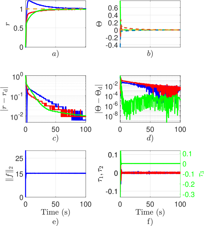
Figure 8: Transferring learning to the Simulink model. Waypoint tracking with the learned controller gains shown in Table LABEL:tab:converged_gains_step. a) position response, b) Euler angles response, c) the magnitude of the force and d) torque applied to the multirotor, respectively.

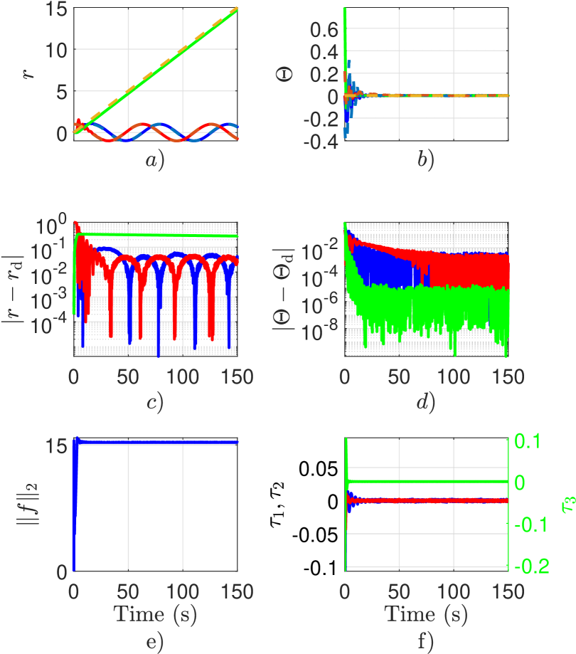
Figure 9: Transferring learning to the Simulink model. Helical trajectory tracking with the learned controller gains shown in Table II. a) position response, b) Euler angles response, c) the magnitude of the force and d) torque applied to the multirotor, respectively.

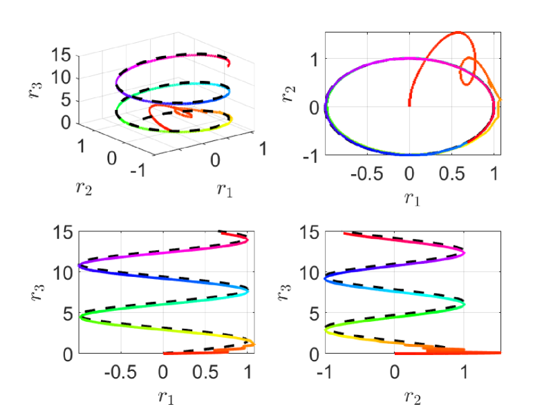
Figure 10: Transferring learning to the Simulink model. Trajectory-tracking response of the Simulink model with the learned controller.

Finally, we investigate the performance of the learned controller experimentally with the Holybro X500 V2 airframe. The physical quadcopter is thus the target environment in the context of transfer learning. In this work, we use the Matlab UAV toolbox package for PX4 autopilot to implement the control architecture shown in Figure 4 in each of the controllers in the inner and the outer loop. The gains used in the nine controllers are shown in Table II. Figures 11 and 12 show the position and Euler angle errors for the waypoint and helical trajectory commands, respectively. Figure 13 shows the trajectory tracking response of the quadcopter to the helical trajectory command. Note that the controller gains learned in the source environment yield a stable controller with acceptable transient performance. Additional tuning of the RCAC hyperparameters in the source environment may yield improved transient performance in the target environment.

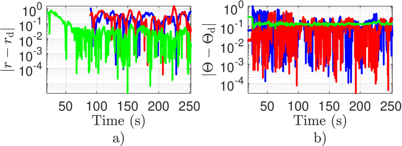
Figure 11: Transferring learning to the X500 quadcopter. Position and Euler angle error response with the X500 quadcopter to a waypoint command.

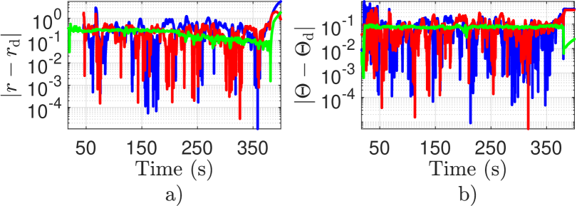
Figure 12: Transferring learning to the X500 quadcopter. Position and Euler angle error response with the X500 quadcopter to a helical trajectory command.

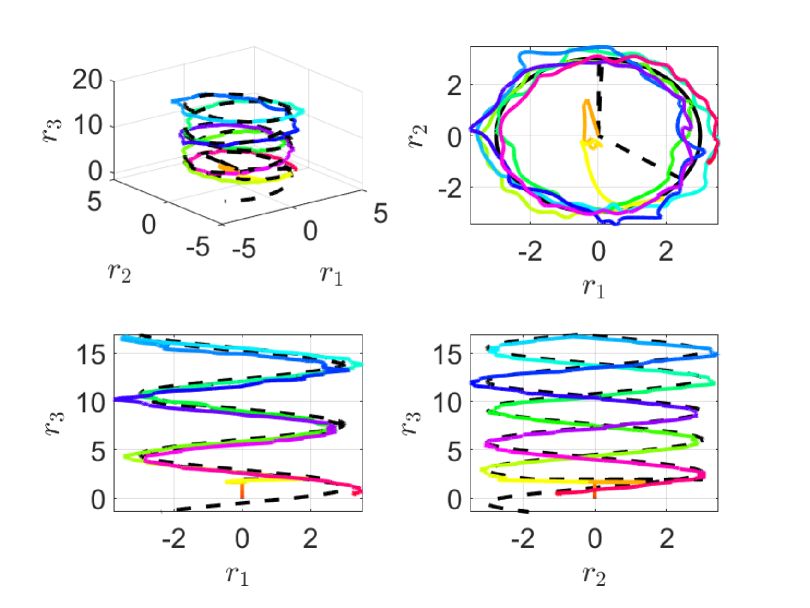
Figure 13: Experimental flight with helical trajectory command. Position response of the X500 quadcopter.

V Conclusions

This paper presented the application of continuous-time retrospective cost adaptive control technique in the transfer learning framework to learn a stabilizing control system for a multirotor in an ideal 12dof model and transfer the learned control system to a realistic multirotor model in the Simulink UAV toolbox and the Holybro X500 V2 quadcopter. In the context of transfer learning, the ideal 12dof model served as the source environment, and the Simulink model and the X500 quadcopter served as the target environment. The inertial properties of the ideal 12dof model were set similar to those of the Holybro X500 V2 quadcopter. This paper showed that the controller gains learned in the source environment yielded a stable controller for the target environment with reasonable transient performance using a single learning experiment without the need to iterate between the source and target environment.

Assessing the quality of the learned controller remains an open problem. Future work is thus focused on developing metrics to quantify the quality and performance of the learned controller as the target system is increasingly different from the source system.

VI Acknowledgement

The authors thank Dr. Juan Augusto Paredes Salazar for insightful comments about transfer learning framework.

References

- [1] Mohammad Fatin Fatihur Rahman, Shurui Fan, Yan Zhang and Lei Chen “A comparative study on application of unmanned aerial vehicle systems in agriculture” In Agriculture 11.1 MDPI, 2021, pp. 22
- [2] Haider AF Almurib, Premeela T Nathan and T Nandha Kumar “Control and path planning of quadrotor aerial vehicles for search and rescue” In SICE Annual Conference 2011, 2011, pp. 700–705 IEEE
- [3] Nathan O Lambert, Daniel S Drew, Joseph Yaconelli, Sergey Levine, Roberto Calandra and Kristofer SJ Pister “Low-level control of a quadrotor with deep model-based reinforcement learning” In IEEE Robotics and Automation Letters 4.4 IEEE, 2019, pp. 4224–4230
- [4] William Koch, Renato Mancuso, Richard West and Azer Bestavros “Reinforcement learning for UAV attitude control” In ACM Transactions on Cyber-Physical Systems 3.2 ACM New York, NY, USA, 2019, pp. 1–21
- [5] Jemin Hwangbo, Inkyu Sa, Roland Siegwart and Marco Hutter “Control of a quadrotor with reinforcement learning” In IEEE Robotics and Automation Letters 2.4 IEEE, 2017, pp. 2096–2103
- [6] Elia Kaufmann, Leonard Bauersfeld, Antonio Loquercio, Matthias Müller, Vladlen Koltun and Davide Scaramuzza “Champion-level drone racing using deep reinforcement learning” In Nature 620.7976 Nature Publishing Group UK London, 2023, pp. 982–987
- [7] Haoran Han, Jian Cheng, Zhilong Xi and Bingcai Yao “Cascade flight control of quadrotors based on deep reinforcement learning” In IEEE Robotics and Automation Letters 7.4 IEEE, 2022, pp. 11134–11141
- [8] Jonas Eschmann, Dario Albani and Giuseppe Loianno “Learning to fly in seconds” In IEEE Robotics and Automation Letters IEEE, 2024
- [9] Daewon Park, Hyona Yu, Nguyen Xuan-Mung, Junyong Lee and Sung Kyung Hong “Multicopter PID attitude controller gain auto-tuning through reinforcement learning neural networks” In Proceedings of the 2019 2nd International Conference on Control and Robot Technology, 2019, pp. 80–84
- [10] Seongheon Lee and Hyochoong Bang “Automatic gain tuning method of a quad-rotor geometric attitude controller using A3C” In International Journal of Aeronautical and Space Sciences 21.2 Springer, 2020, pp. 469–478
- [11] Seif-El-Islam Hasseni, Latifa Abdou and Hossam-Eddine Glida “Parameters tuning of a quadrotor PID controllers by using nature-inspired algorithms” In Evolutionary Intelligence 14.1 Springer, 2021, pp. 61–73
- [12] Sheng Cheng, Minkyung Kim, Lin Song, Chengyu Yang, Yiquan Jin, Shenlong Wang and Naira Hovakimyan “Difftune: Auto-tuning through auto-differentiation” In IEEE Transactions on Robotics IEEE, 2024
- [13] Yousaf Rahman, Antai Xie and Dennis S. Bernstein “Retrospective Cost Adaptive Control: Pole Placement, Frequency Response, and Connections with LQG Control” In IEEE Control System Magazine 37, 2017, pp. 28–69 DOI: 10.1109/MCS.2017.2718825
- [14] Mohammadreza Kamaldar, Syed Aseem U. Islam, Sneha Sanjeevini, Ankit Goel, Jesse B. Hoagg and Dennis S. Bernstein “Adaptive digital PID control of first-order-lag-plus-dead-time dynamics with sensor, actuator, and feedback nonlinearities” In Advanced Control for Applications 1.1, 2019, pp. e20 DOI: 10.1002/adc2.20
- [15] Ankit Goel, Juan Augusto Paredes, Harshil Dadhaniya, Syed Aseem Ul Islam, Abdulazeez Mohammed Salim, Sai Ravela and Dennis Bernstein “Experimental implementation of an adaptive digital autopilot” In 2021 American Control Conference (ACC), 2021, pp. 3737–3742 IEEE
- [16] John Spencer, Joonghyun Lee, Juan Augusto Paredes, Ankit Goel and Dennis Bernstein “An adaptive PID autotuner for multicopters with experimental results” In Proc. Int. Conf. Rob. Autom., 2022, pp. 7846–7853 IEEE
- [17] Karl Weiss, Taghi M Khoshgoftaar and DingDing Wang “A survey of transfer learning” In Journal of Big data 3 Springer, 2016, pp. 1–40
- [18] Ankit Goel, Abdulazeez Mohammed Salim, Ahmad Ansari, Sai Ravela and Dennis Bernstein “Adaptive digital pid control of a quadcopter with unknown dynamics” In arXiv preprint arXiv:2006.00416, 2020
- [19] A. Goel, S.. U. Islam and D.. Bernstein “Adaptive Control of MIMO Systems Using Sparsely Parameterized Controllers” In 2020 American Control Conference (ACC), 2020, pp. 5340–5345 DOI: 10.23919/ACC45564.2020.9147513
- [20] Mathworks “Simulink-Based Plant Model”, 2024 URL: https://www.mathworks.com/help/uav/px4/ref/simulator-plant-model-example.html#d126e14320