P1-KAN an effective Kolmogorov Arnold Network for function approximation
Abstract.
A new Kolmogorov-Arnold network (KAN) is proposed to approximate potentially irregular functions in high dimension. We show that it outperforms multilayer perceptrons in terms of accuracy and converges faster. We also compare it with several proposed KAN networks: the original spline-based KAN network appears to be more effective for smooth functions, while the P1-KAN network is more effective for irregular functions.
1. Introduction
Kolmogorov Arnold Networks [14], based on Arnold Kolmogorov representation theorem, have recently been proposed instead of multilayer perceptrons to approximate functions in high dimension: Arnold and Kolmogorov showed long ago [10] that a multivariate continuous smooth function on a bounded domain can be written as a finite composition of the sum of continuous functions of a single variable. More precisely, if is smooth on , then
| (1) |
where and .
As the 1D functions can very irregular or even fractal, it has been shown that they may not be learnable in practice [8, 15].
To overcome this limitation, [14] propose to extend this representation.
First they propose not to stick to terms in the outer sum in (1) and to define a KAN layer as an operator from to :
| (2) |
Second, by stacking the layers, i.e; composing the operator , they define the KAN operator from to :
| (3) |
Since all functions are one dimensional, many classical methods are available to propose an easy to implement approximation.
In their proposed implementation, [14] use B spline (see for example [4]) associated with the SILU activation function to approximate the function : the spline coefficients and the multiplicative coefficient of the SILU function are learned using a classical stochastic gradient algorithm as done with MLPs.
This network has been rapidly tested replacing MPLs in transformers [24] for example and
in various fields : medical sector in [9], vision [5, 12], time series [21].
Strengths and weaknesses of this approach compared to MLPs are discussed in [25] and, depending on its used, its to superiority to MLPs is not always obvious [17, 11].
Following this first article, different evolutions of this architecture are proposed to address different problems :[6] proposes an evolution of the algorithm to replace LSTM in time series, [23] for Graph Collaborative Filtering, [2] for convolutional networks, [1] in mechanics.
The original spline-based algorithm has several drawbacks.
The first disadvantage of this approach is that the spline approximation is expensive at least in the original algorithm proposed.
The second is that the output of a layer may not be in the grid initially chosen for the following layer: the authors propose to adapt the grid during the iterations to the output of the previous layer, which still increases the complexity and the computational cost of the procedure. Finally, since the Kolmogorv representation theorem involves a very irregular function, one may wonder whether it is interesting to use a rather high order approximation as a spline.
To address the first point, many other approximations based on classical numerical analysis have been proposed using: wavelets [3], radial basis [13, 20] which reduces the computation time by 3, Chebyshev polynomials [19] and many others. An interesting representation that leads to a very effective layer is the ReLU-KAN [16] [18], which is based only on the ReLU function, matrix addition and multiplication, and divides the computation time by 20.
To address the second point, some use a sigmoid activation function [19] to get an output in , others use some adaptation of the support of the basis functions by trying to learn them [16].
Concerned by the possibility of KANs to approximate high dimensional functions in high dimension, especially for stochastic optimisation purposes in [7],[22], we have tested the ReLU-KAN network, sometimes obtaining excellent results in the optimisation of complex hydraulic valleys and sometimes experiencing divergence.
In order to avoid this divergence problem observed in operational problems, we have developed the P1-KAN network, borrowing some interesting features from the ReLU-KAN, but clearly defining the support of the layer function and avoiding the network adaptation proposed in [14]. In the first part of the article we describe our architecture.
In a second part, we compare it with MLPs, Spline-KAN, Radial basis KAN and ReLU-KAN on function approximation using either regular or very irregular functions in different dimensions.
2. The P1-KAN Network
We will first explain the main features of the method, and then go into detail about the algorithm and why P1-KAN is different from other KAN networks.
2.1. The P1-KAN Layer
We will first explain the main features of the method, and then go into detail about the algorithm and why P1-KAN is different from other KAN networks.
2.2. The P1-KAN Layer
We assume that the layer is an operator with support described by and with values in . As for the classical KAN layers, a number of meshes per direction are used to discretize , giving the mesh vertices of trainable variables in . Set , , the function in (2) is defined using a P1 finite element method: for ,
| (4) |
where are also trainable variables and is the basis of the shape function with compact support in each interval for and defined as:
| (7) | |||
| (8) |
for .
Similarly, (or ) is defined as a linear by-part function with support (or ) and such that (or ).
Unlike other networks, the P1-KAN layer, which is theoretically described as an operator from to by the equation
(2), takes as input not only a sample but also the description of the support .
In detail, the vertices in are generated for each direction for by
| (9) |
where the matrix has elements in . The operator value is given by:
| (10) |
The tensor and are the trainable variables of the network.
As output, the layer returns the values of in
and the lattice obtained from the possible values.
Due to the use of the finite element approximation, this output lattice is exactly obtained from the tensor by:
for .
2.3. The global P1-KAN network
As shown in the previous section, the P1-KAN layer inputs values and a hypercube, and it outputs the values obtained by the operator and a hypercube. Therefore, it is natural to stack the layers without using any grid adaptation or using any sigmoid function to send the output of the layer back to a known bounded domain.
The P1-KAN network takes for the initial hypercube used for the first layer a hypercube corresponding to the bounded domain where we want to approximate the unknown function.
An implementation in Tensorflow is available at https://fime-lab.org/warin-xavier.
3. Numerical results
In this section we compare the classical feedforward network with Spline-KAN [14], Fast-KAN [13], ReLU-KAN [13] and P1-KAN on two types of functions defined on .
-
A
The first function is regular but very fast oscillating with increasing dimension and is defined for
(11) where . The function in 2D is given in figure 1.
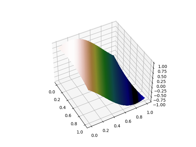
Figure 1. Function A in 2D -
B
The second is a very irregular one and is given as
(12) where and is applied component by component. The function is shown in 2D in figure 2.
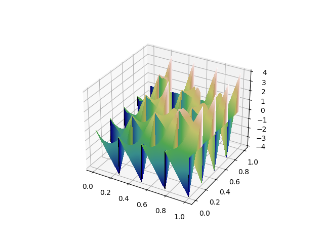
Figure 2. Function B in 2D
To approximate a function with a neural network we use the classical quadratic loss function defined as:
and where is a uniform random variable on .
Using a stochastic gradient algorithm with the ADAM optimizer, a learning rate of , and a batch size of , we minimize the loss .
The MLPs use a ReLU activation function, using either 2 layers with 10, 20, 40 neurons for each layer or 3 layers with 10, 20, 40, 80, 160 neurons:
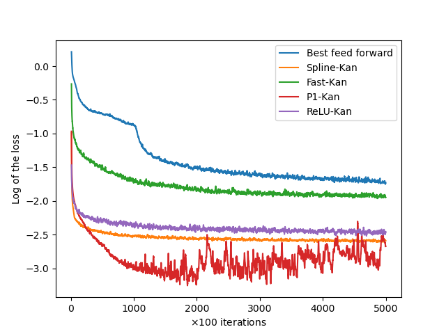
In each case, the MLP are optimized by varying the number of neurons and layers, and only the result that gives the smallest loss during the iterations is kept for the plots.
The different KAN networks are compared using the same parameterization (number of hidden layers, number of neurons, number of meshes used for the 1D functions). The ReLU-KAN has an additional parameter , which we keep at as suggested in the original article.
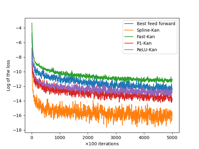
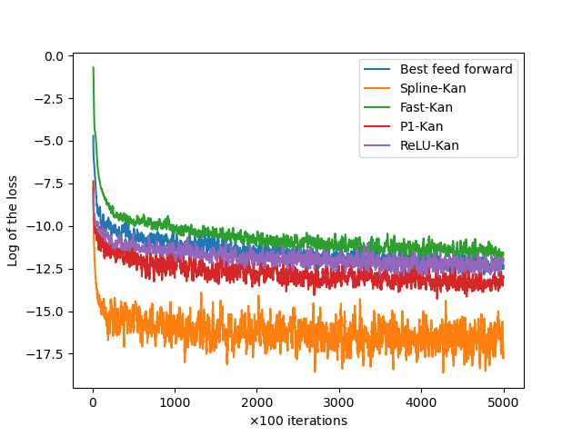
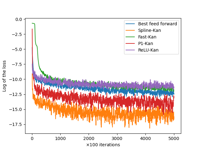
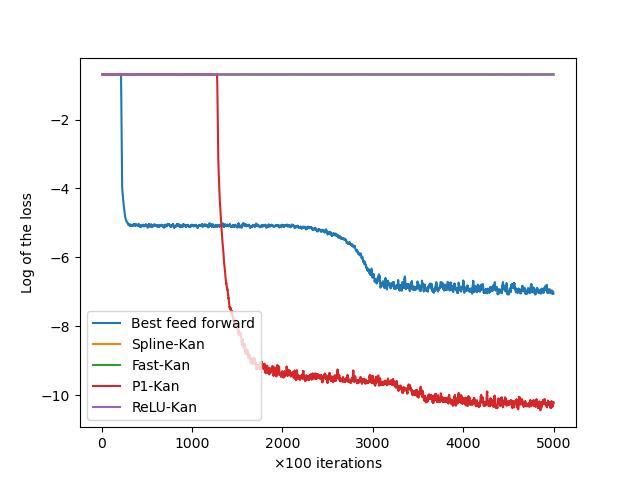
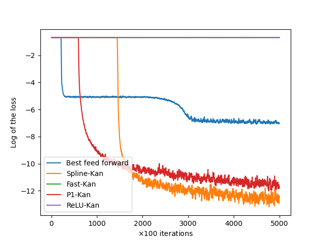
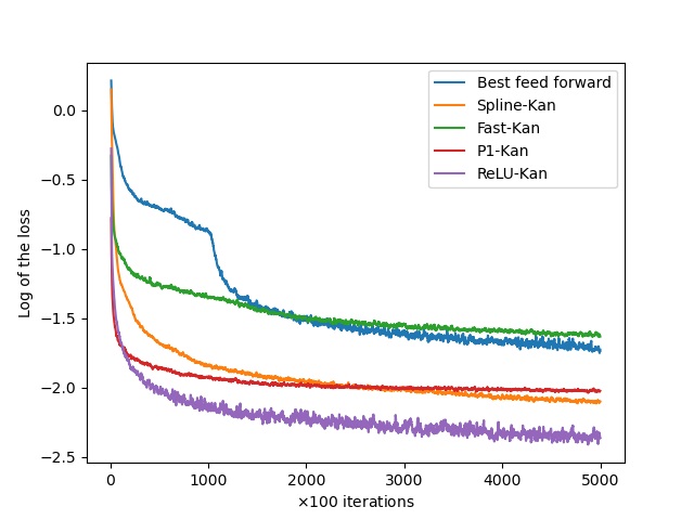
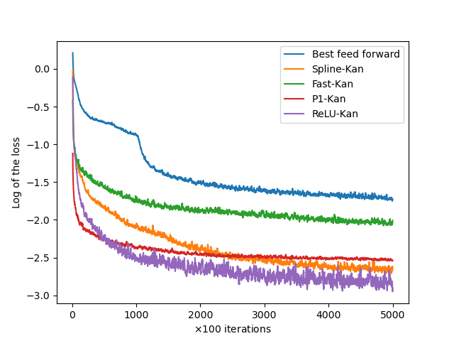
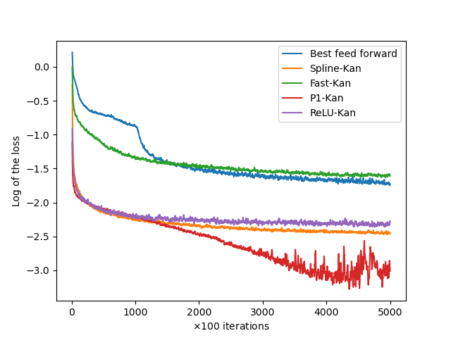
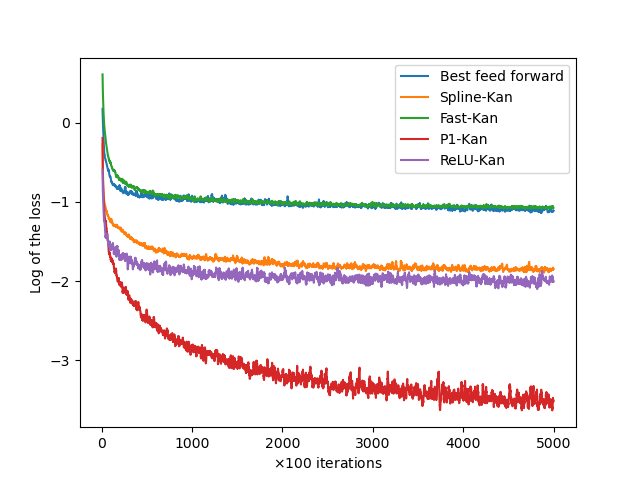
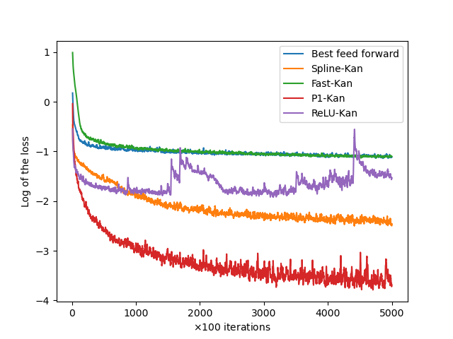
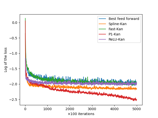
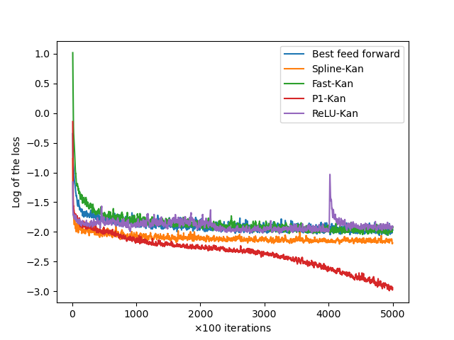
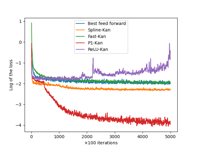
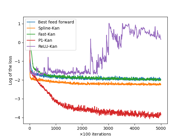
For all plots, every 100 gradient iterations, the loss is calculated more accurately using samples, giving a series of log-losses plotted using a moving average window of 10 results.
ReLU-KAN is very efficient in terms of computation time as it can be broken down into a few operations involving only the ReLU function, matrix addition and multiplication.
On a 11th generation Intel(R) Core(TM) i7-11850H @ 2.50GHz, using the same parameterisation of the KAN nets, the P1-KAN computation time is between 1.5 and 2 times slower than the ReLU-KAN.
For the spline version of the KAN originally from [14], we use the efficient Pytorch KAN implementation.
For the Fast-KAN [13], we use the Pytorch implementation.
3.1. Results for the A function
The results in dimension 6 shown in figure 3 indicate that the original Spline KAN network converges faster than the P1-KAN network which is the second more effective network. In general, the ReLU-KAN network converges at least as well as the best feedforward, while the Fast-KAN is the less effective network.
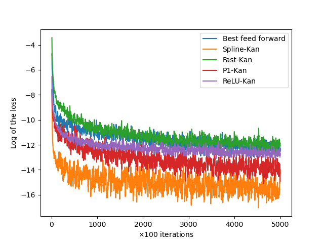
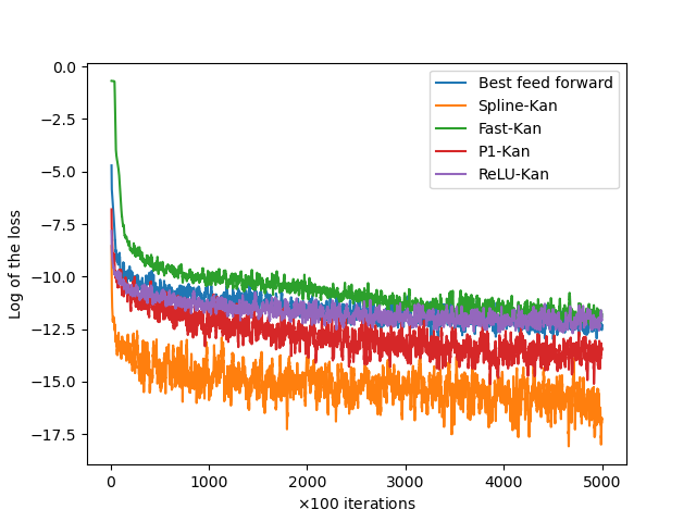
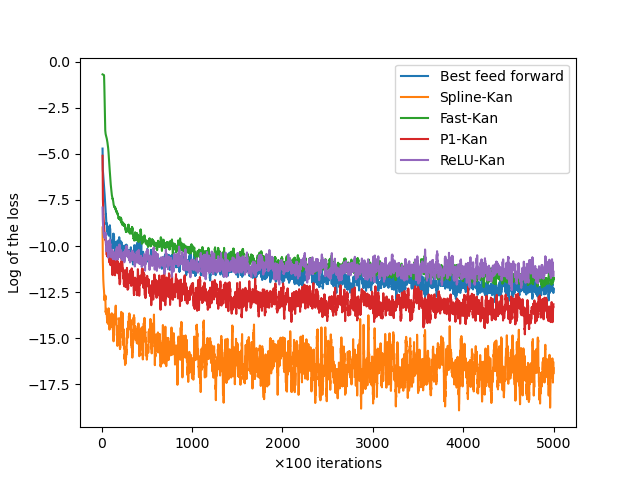
In dimension 12 on figure 4, the Spline-KAN and the P1-KAN again give the best results. The Fast-KAN and the ReLU-KAN fail, while the feedforward network seems to converge very slowly and its accuracy remains limited. Notice that the P1-KAN give good results when is small, but doesn’t give any results when is too large.
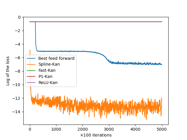
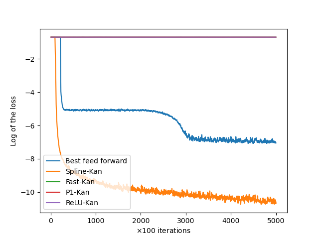
In dimension 13 on figure 5, only the Spline-KAN and P1-KAN networks succeed but not on every configuration.
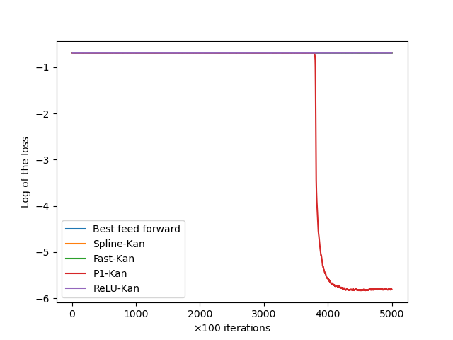
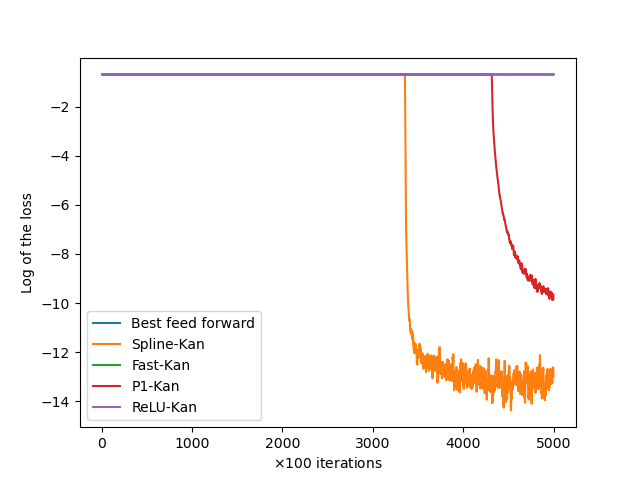
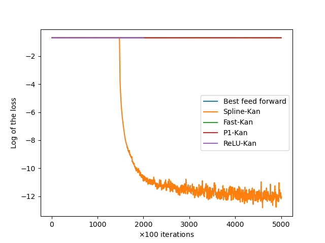
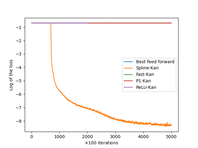
These results indicate that for complex smooth functions, the Spline-KAN is the most effective but the P1-KAN network is still very effective when is kept small.
3.2. Results for the B function
In dimension 2 on figure 6, we see that the feedforward lags behind the KAN networks. By taking high values of , P1-KAN is the only network that gives very good results. The Spline-KAN is the second best network.
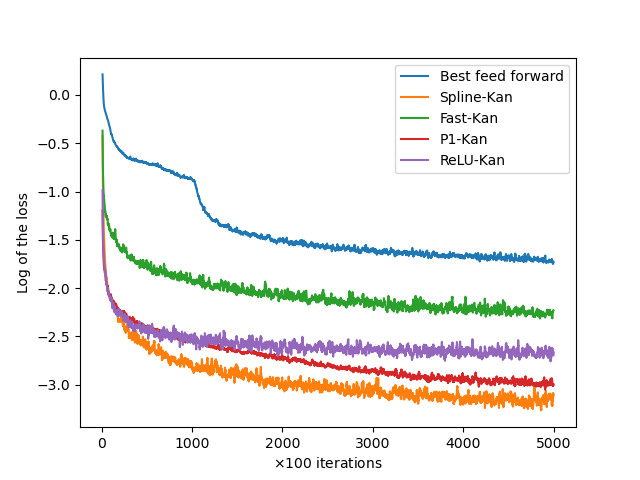
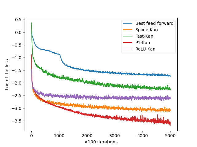
The previous results are confirmed in dimension 3 in figure 6: the P1-KAN clearly gives the best results. We can see that in some configurations the ReLU-KAN network can face some converge problems.
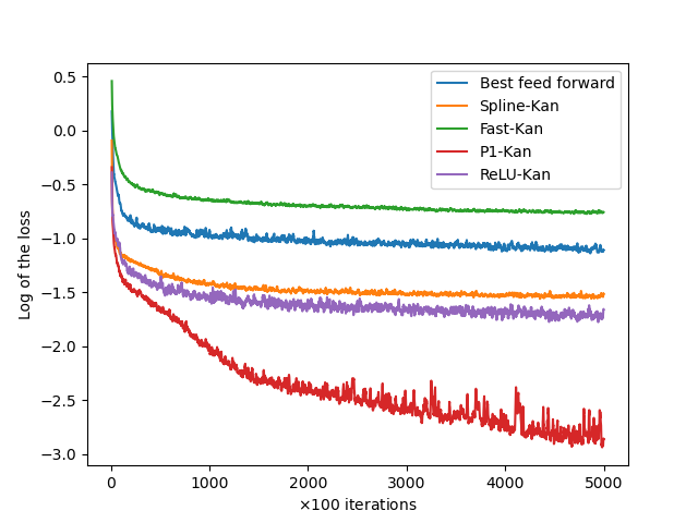
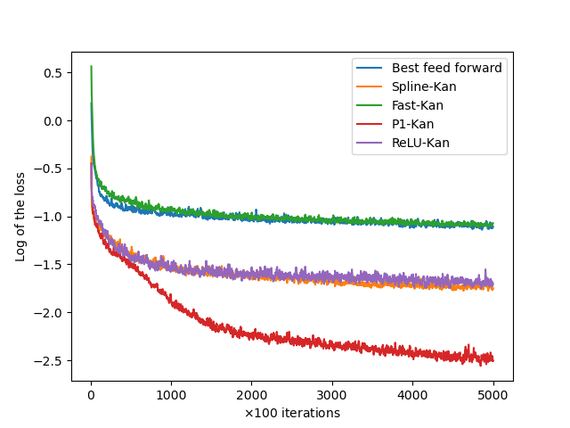
Finally, if we go up to dimension 5, we see that the ReLU-KAN network can diverge. The P1-KAN network is the only one that gives acceptable results by using 2 or 3 hidden layers of 10 neurons and .
4. Conclusion
The P1-KAN seems to be an excellent network for approximating functions. When the function to be approximated is smooth, it is not as effective as the Spline-KAN, but it is most effective when the function to be approximated is irregular. We were able to reproduce on simple examples the divergence problems encountered with the ReLU-KAN on operational problems in the optimization of complex hydraulic valleys. Further comparisons using MLPs and KANs to optimize French hydraulic valleys will be presented in a forthcoming article.
References
- [1] Diab W Abueidda, Panos Pantidis, and Mostafa E Mobasher. Deepokan: Deep operator network based on kolmogorov arnold networks for mechanics problems. arXiv preprint arXiv:2405.19143, 2024.
- [2] Alexander Dylan Bodner, Antonio Santiago Tepsich, Jack Natan Spolski, and Santiago Pourteau. Convolutional kolmogorov-arnold networks. arXiv preprint arXiv:2406.13155, 2024.
- [3] Zavareh Bozorgasl and Hao Chen. Wav-kan: Wavelet kolmogorov-arnold networks. arXiv preprint arXiv:2405.12832, 2024.
- [4] Arindam Chaudhuri. B-splines. arXiv preprint arXiv:2108.06617, 2021.
- [5] Minjong Cheon. Demonstrating the efficacy of kolmogorov-arnold networks in vision tasks. arXiv preprint arXiv:2406.14916, 2024.
- [6] Remi Genet and Hugo Inzirillo. Tkan: Temporal kolmogorov-arnold networks. arXiv preprint arXiv:2405.07344, 2024.
- [7] Maximilien Germain, Huyên Pham, Xavier Warin, et al. Neural networks-based algorithms for stochastic control and pdes in finance. arXiv preprint arXiv:2101.08068, 2021.
- [8] Federico Girosi and Tomaso Poggio. Representation properties of networks: Kolmogorov’s theorem is irrelevant. Neural Computation, 1(4):465–469, 1989.
- [9] William Knottenbelt, Zeyu Gao, Rebecca Wray, Woody Zhidong Zhang, Jiashuai Liu, and Mireia Crispin-Ortuzar. Coxkan: Kolmogorov-arnold networks for interpretable, high-performance survival analysis. arXiv preprint arXiv:2409.04290, 2024.
- [10] Andrei Nikolaevich Kolmogorov. On the representation of continuous functions of several variables by superpositions of continuous functions of a smaller number of variables. American Mathematical Society, 1961.
- [11] Tran Xuan Hieu Le, Thi Diem Tran, Hoai Luan Pham, Vu Trung Duong Le, Tuan Hai Vu, Van Tinh Nguyen, Yasuhiko Nakashima, et al. Exploring the limitations of kolmogorov-arnold networks in classification: Insights to software training and hardware implementation. arXiv preprint arXiv:2407.17790, 2024.
- [12] Chenxin Li, Xinyu Liu, Wuyang Li, Cheng Wang, Hengyu Liu, and Yixuan Yuan. U-kan makes strong backbone for medical image segmentation and generation. arXiv preprint arXiv:2406.02918, 2024.
- [13] Ziyao Li. Kolmogorov-arnold networks are radial basis function networks. 2024.
- [14] Ziming Liu, Yixuan Wang, Sachin Vaidya, Fabian Ruehle, James Halverson, Marin Soljačić, Thomas Y Hou, and Max Tegmark. Kan: Kolmogorov-arnold networks. arXiv preprint arXiv:2404.19756, 2024.
- [15] Tomaso Poggio, Andrzej Banburski, and Qianli Liao. Theoretical issues in deep networks. Proceedings of the National Academy of Sciences, 117(48):30039–30045, 2020.
- [16] Qi Qiu, Tao Zhu, Helin Gong, Liming Chen, and Huansheng Ning. Relu-kan: New kolmogorov-arnold networks that only need matrix addition, dot multiplication, and relu. arXiv preprint arXiv:2406.02075, 2024.
- [17] Haoran Shen, Chen Zeng, Jiahui Wang, and Qiao Wang. Reduced effectiveness of kolmogorov-arnold networks on functions with noise. arXiv preprint arXiv:2407.14882, 2024.
- [18] Chi Chiu So and Siu Pang Yung. Higher-order-relu-kans (hrkans) for solving physics-informed neural networks (pinns) more accurately, robustly and faster. arXiv preprint arXiv:2409.14248, 2024.
- [19] Sidharth SS. Chebyshev polynomial-based kolmogorov-arnold networks: An efficient architecture for nonlinear function approximation. arXiv preprint arXiv:2405.07200, 2024.
- [20] Hoang-Thang Ta. Bsrbf-kan: A combination of b-splines and radial basic functions in kolmogorov-arnold networks. arXiv preprint arXiv:2406.11173, 2024.
- [21] Cristian J Vaca-Rubio, Luis Blanco, Roberto Pereira, and Màrius Caus. Kolmogorov-arnold networks (kans) for time series analysis. arXiv preprint arXiv:2405.08790, 2024.
- [22] Xavier Warin. Reservoir optimization and machine learning methods. EURO Journal on Computational Optimization, 11:100068, 2023.
- [23] Jinfeng Xu, Zheyu Chen, Jinze Li, Shuo Yang, Wei Wang, Xiping Hu, and Edith C-H Ngai. Fourierkan-gcf: Fourier kolmogorov-arnold network–an effective and efficient feature transformation for graph collaborative filtering. arXiv preprint arXiv:2406.01034, 2024.
- [24] Xingyi Yang and Xinchao Wang. Kolmogorov-arnold transformer. arXiv preprint arXiv:2409.10594, 2024.
- [25] Runpeng Yu, Weihao Yu, and Xinchao Wang. Kan or mlp: A fairer comparison. arXiv preprint arXiv:2407.16674, 2024.