Geodesics and Global Properties of the Liouville Solution in General Relativity with a Scalar Field

Abstract

One parameter family of exact solutions in general relativity with a scalar field has been found using the Liouville metric. The scalar field potential is exponential and bounded from below. This model is interesting because, in particular, the solution corresponding to the naked singularity provides smooth extension of the Friedmann universe with accelerated expansion through the zero of the scale factor back in time. There is also nonstatic solution describing a black hole formation. All geodesics are found explicitly. Their analysis shows that the Liouville solutions are global ones: every geodesic is either continued to infinite value of the canonical parameter in both directions or ends up at the singularity at its finite value.

1 Introduction

Exact solutions of Einstein’s equations always attract much interest of physicists and mathematicians. Though many exact solutions are known (see e.g [1, 2]), this field of research have still many surprises.

Recently we have found a new (Liouville) exact solution in General Relativity minimally coupled to a scalar field with arbitrary potential bounded from below [3]. Two assumptions were made: (i) the metric is of Liouville type, i.e. it is conformally flat, the conformal factor being the sum of arbitrary functions depending on single coordinates, and (ii) the scalar field depends on coordinates only through the conformal factor. The corresponding general solution to the field equations depends on one parameter and is very simple. It is invariant under global Lorentz transformations and, therefore, admits six noncommuting Killing vector fields. Note, that symmetry of the space-time was not assumed from the very beginning but arises as the consequence of the field equations (spontaneous symmetry emergence [4, 5]). Despite the mathematical simplicity, the solution is of considerable interest to physics. The obtained solutions describe, in particular, the black hole formation by the scalar field and the naked singularity.

Note an interesting feature of the naked singularity solution. Namely, it can be transformed into the Friedmann form only inside the light cone, where it describes the accelerated expansion of the homogeneous and isotropic universe with constant negative curvature space sections. The scale factor is equal to zero on the light cone, which is geodesically incomplete. Global analysis shows, that each geodesic crosses this light cone at finite value of the canonical parameter. Thus, the Liouville solution provides smooth continuation of the cosmological solution through the zero of the scale factor back in time either to the naked singularity or to the past time infinity. We believe, that this is the first example describing a smooth extension of the accelerated expansion through the hyper-surface of zeroes of the conformal factor.

The solution exists only for the special exponential type of the scalar field potential bounded from below. Such potentials attract much interest, though they have some difficulties in quantization. They arise in higher-dimensional gravity models, superstring and M-theory (see, e.g. [6, 7]) and are used in cosmological models [8, 9, 10].

The Liouville metric admits complete separation of variables in the Hamilton–Jacobi equation for geodesics. It means that the geodesic equations are Liouville integrable (have four independent envolutive conservation laws which are quadratic in momenta). That is there are four independent Killing tensors of second rank.

In the present paper, we integrate explicitly geodesic equations and prove that the obtained Liouville solution is a global one: every geodesic can be either extended to infinite value of the canonical parameter in both directions or reaches singularity at its finite value.

For convenience of the reader, we repeat the derivation of the Liouville solution, which is quite short, with minor extensions at the beginning of the paper.

2 Notation and solution

We consider four-dimensional space-time ${\mathbb{M}}$ with coordinates $x=(x^{\alpha})$, $\alpha=0,1,2,3$. Let there be the Liouville metric

$$g_{\alpha\beta}:=\Phi(x)\eta_{\alpha\beta},\qquad\eta_{\alpha\beta}:=\text{\sf\,\small diag\,}(+1,-1,-1,-1),$$ (1)

where the conformal factor is the sum of four arbitrary functions on single arguments

$$\Phi(x):=\phi_{0}(x^{0})+\phi_{1}(x^{1})+\phi_{2}(x^{3})+\phi_{3}(x^{3}),\qquad\Phi\neq 0.$$ (2)

This is the famous Liouville metric [11] well known in mechanics, because it admits complete separation of variables in the Hamilton–Jacobi equations for geodesic lines even if arbitrary functions are not specified. For some choices of arbitrary functions, metric (1) is symmetric. For example, if all functions are constant then we have the usual Lorentz metric up to rescaling of coordinates. There is also such choice of functions that the Liouville metric becomes spherically symmetric (see below). However, metric (1) in a general situation has no Killing vectors. It means that geodesic equations are Liouville integrable even if there is no symmetry at all. Moreover the variables in the wave and Dirac equation on a manifold with metric (1) are also completely separated (with minor corrections). Thus, the Liouville metric is of particular interest.

The Liouville metric (1) is conformally flat, its Weyl tensor vanishes, and, therefore, its curvature tensor is of type 0 in Petrov’s classification [12].

Christoffel’s symbols for metric (1) are

$$\Gamma_{\alpha\beta}{}^{\gamma}:= \frac{1}{2}\big{(}\partial_{\alpha}g_{\beta\delta}+\partial_{\beta}g_{\alpha\delta}-\partial_{\delta}g_{\alpha\beta}\big{)}g^{\delta\gamma}=$$

$$= \frac{1}{2\Phi}\big{(}\phi^{\prime}_{\alpha}\delta_{\beta}^{\gamma}+\phi^{\prime}_{\beta}\delta_{\alpha}^{\gamma}-\phi^{\prime\gamma}\eta_{\alpha\beta}\big{)}.$$ (3)

Here and in what follows raising and lowering of indices are performed by the Lorentz metric $\eta_{\alpha\beta}$ which is fixed once and forever, and the prime denotes the derivative with respect to the corresponding arguments. The curvature and Ricci tensors and scalar curvature have the form

$$R_{\alpha\beta\gamma}{}^{\delta}:= \partial_{\alpha}\Gamma_{\beta\gamma}{}^{\delta}-\partial_{\beta}\Gamma_{\alpha\gamma}{}^{\delta}-\Gamma_{\alpha\gamma}{}^{\epsilon}\Gamma_{\beta\epsilon}{}^{\delta}+\Gamma_{\beta\gamma}{}^{\epsilon}\Gamma_{\alpha\epsilon}{}^{\delta}=$$ (4)

$$= \frac{1}{2\Phi}\big{(}\Phi^{\prime\prime}_{\alpha\gamma}\delta_{\beta}^{\delta}-\Phi^{\prime\prime}_{\beta\gamma}\delta_{\alpha}^{\delta}-\Phi^{\prime\prime}_{\alpha}{}^{\delta}\eta_{\beta\gamma}+\Phi^{\prime\prime}_{\beta}{}^{\delta}\eta_{\alpha\gamma}\big{)}+$$

$$+\frac{3}{4\Phi^{2}}\big{(}-\phi^{\prime}_{\alpha}\phi^{\prime}_{\gamma}\delta_{\beta}^{\delta}+\phi^{\prime}_{\beta}\phi^{\prime}_{\gamma}\delta_{\alpha}^{\delta}+\phi^{\prime}_{\alpha}\phi^{\prime\delta}\eta_{\beta\gamma}-\phi^{\prime}_{\beta}\phi^{\prime\delta}\eta_{\alpha\gamma}\big{)}+$$

$$+\frac{1}{4\Phi^{2}}\phi^{\prime}_{\epsilon}\phi^{\prime\epsilon}\big{(}\eta_{\alpha\gamma}\delta_{\beta}^{\delta}-\eta_{\beta\gamma}\delta_{\alpha}^{\delta}\big{)},$$

$$R_{\alpha\gamma}:= R_{\alpha\beta\gamma}{}^{\beta}=\frac{1}{2\Phi}\big{(}2\Phi^{\prime\prime}_{\alpha\gamma}+\Phi^{\prime\prime}_{\epsilon}{}^{\epsilon}\eta_{\alpha\gamma}\big{)}-\frac{3}{2\Phi^{2}}\phi^{\prime}_{\alpha}\phi^{\prime}_{\gamma},$$ (5)

$$R:= g^{\alpha\gamma}R_{\alpha\gamma}=\frac{3}{\Phi^{2}}\Phi^{\prime\prime}_{\alpha}{}^{\alpha}-\frac{3}{2\Phi^{3}}\phi^{\prime}_{\alpha}\phi^{\prime\alpha}.$$ (6)

If $\Phi>0$, then the signature of the metric is $(+---)$, and a scalar field $\varphi(x)$ in General Relativity with cosmological constant $\Lambda$ is described by the standard action

$$S:=\int\!dx\sqrt{{\scriptstyle|}g{\scriptstyle|}}\left[R-2\Lambda+\frac{1}{2}g^{\alpha\beta}\partial_{\alpha}\varphi\partial_{\beta}\varphi-V(\varphi)\right],\qquad g:=\text{\sf\,\small\, det\,}g_{\alpha\beta},$$ (7)

where the potential for a scalar field $V(\varphi)$ will be specified later. The signs in the action are chosen in such a way that there are no ghosts for $\Phi>0$. For another choice of the metric signature $(-+++)$, we have to change signs of the scalar curvature and kinetic term for a scalar field to avoid ghosts. Then the conformal factor in Liouville metric (1) has to be replaced by $\Phi<0$, keeping Lorentz metric $\eta_{\alpha\beta}$ unchanged.

First, we consider metrics of signature $(+---)$ corresponding to positive conformal factor $\Phi>0$.

Variation of this action with respect to all metric components $g_{\alpha\beta}$ and a scalar field $\varphi(x)$ yields the field equations. For the Liouville metric (1), (2), they are

$$R_{\alpha\beta}=-\frac{1}{2}\partial_{\alpha}\varphi\partial_{\beta}\varphi+\frac{1}{2}\Phi\eta_{\alpha\beta}(V+2\Lambda),$$ (8)

$$\eta^{\alpha\beta}\partial^{2}_{\alpha\beta}\varphi+\frac{1}{\Phi}\phi^{\prime\alpha}\partial_{\alpha}\varphi+\Phi V^{\prime}=0,$$ (9)

which are to be solved.

We shall look for solutions of the field equations assuming that the scalar field depends on coordinates only through the conformal factor, $\varphi(x):=\Psi\big{(}\Phi(x)\big{)}$, where $\Psi\big{(}\Phi\big{)}$ is an arbitrary function of single argument. Then equation (8) for $\alpha\neq\beta$ implies

$$\frac{3\phi^{\prime}_{\alpha}\phi^{\prime}_{\beta}}{\Phi^{2}}=\Psi^{\prime 2}\phi^{\prime}_{\alpha}\phi^{\prime}_{\beta},$$

where $\Psi^{\prime}:=d\Psi/d\Phi$. Therefore, function $\Psi$ satisfies equation

$$\Psi^{\prime 2}=\frac{3}{\Phi^{2}}$$

for nonconstant functions $\phi^{\prime}_{\alpha}\neq 0$. Its general solution is

$$\varphi:=\Psi=\pm\sqrt{3}\text{\sf\small\, ln}\big{(}C\Phi\big{)}\qquad\Leftrightarrow\qquad C\Phi=\text{\sf\small\,e}^{\pm\varphi/\sqrt{3}},$$ (10)

where $C$ is an arbitrary integration constant such that $C\Phi>0$. Then Eqs. (8), (9) reduce to overdetermined system of equations

$$\Phi^{\prime\prime}_{\alpha\beta}+\frac{1}{2}\Phi^{\prime\prime}_{\gamma}{}^{\gamma}\eta_{\alpha\beta}= \frac{1}{2}\eta_{\alpha\beta}\Phi^{2}(V+2\Lambda),$$ (11)

$$\Phi^{\prime\prime}_{\gamma}{}^{\gamma}\pm\frac{\Phi^{2}}{\sqrt{3}}V^{\prime}= 0.$$ (12)

Taking the trace of Eq. (11) we obtain

$$3\Phi^{\prime\prime}_{\gamma}{}^{\gamma}=2\Phi^{2}(V+2\Lambda).$$ (13)

This equation coincides with Eq. (12) only if the potential satisfies the differential equation

$$V+2\Lambda\pm\frac{\sqrt{3}}{2}V^{\prime}=0.$$ (14)

It has a general solution

$$|V+2\Lambda|=\text{\sf\small\,e}^{\mp\frac{2}{\sqrt{3}}(\varphi+\varphi_{0})},$$

where $\varphi_{0}$ is an integration constant. Assuming that the potential is bounded from below and this relation holds for all $\varphi$ the modulus sign can be dropped. So, the potential is

$$V=-2\Lambda+\text{\sf\small\,e}^{\mp\frac{2}{\sqrt{3}}(\varphi+\varphi_{0})}.$$ (15)

Now the only equation which has to be solved is Eq. (11). It takes the form

$$\Phi^{\prime\prime}_{\alpha\beta}=\frac{1}{6}\eta_{\alpha\beta}\Phi^{2}(V+2\Lambda).$$ (16)

For the Liouville conformal factor (2), $\Phi^{\prime\prime}_{\alpha\beta}\equiv 0$ when $\alpha\neq\beta$. Therefore, off diagonal components of this equation are satisfied. The diagonal components reduce to

$$\begin{split}\phi^{\prime\prime}_{0}=&~{}~{}\frac{1}{6}\Phi^{2}(V+2\Lambda),\\ \phi^{\prime\prime}_{i}=&-\frac{1}{6}\Phi^{2}(V+2\Lambda),\qquad i=1,2,3.\end{split}$$

Taking the sum of these equations we get

$$\phi^{\prime\prime}_{0}+\phi^{\prime\prime}_{i}=0,\qquad\forall i.$$

The summands depend on different arguments and hence are equal to the same positive constant $b_{0}$ for $\Phi>0$ with opposite signs. Therefore,

$$\begin{split}\phi_{0}=&~{}~{}b_{0}\big{(}x^{0}-x^{0}_{0}\big{)}^{2}+c_{0},\\ \phi_{i}=&-b_{0}\big{(}x^{i}-x^{i}_{0}\big{)}^{2}+c_{i},\end{split}$$ (17)

where $x^{\alpha}_{0}$ and $c_{\alpha}$ are arbitrary integration constants. Shifting the coordinates we put $x^{\alpha}_{0}=0$. Moreover, rescaling the coordinates $x^{\alpha}\mapsto kx^{\alpha}$, where $k:=b_{0}^{-1/4}$, constant $b_{0}$ can be set to unity, $b_{0}=1$. Hence, the conformal factor is the Lorentz invariant quadratic polynomial:

$$\Phi=s+c,$$ (18)

where

$$s:=\eta_{\alpha\beta}x^{\alpha}x^{\beta},\qquad c:=c_{0}+c_{1}+c_{2}+c_{3}\in{\mathbb{R}}.$$

Now Eq. (16) reduces to

$$2=\frac{1}{6}\Phi^{2}(V+2\Lambda),$$ (19)

and Eq. (12) becomes

$$2=\frac{1}{6C^{2}},$$ (20)

where Eqs. (10) and (15) were used. It defines constant $C$ in ansatz (10).

Thus, the particular solution of field equations (8) and (9) with ansatz $\varphi:=\Psi(\Phi)$ has been found. The solution is very simple: the conformal factor in the Liouville metric is given by Eq. (18) and the scalar field is

$$\varphi=\pm\sqrt{3}\text{\sf\small\, ln}\left(\frac{\Phi}{2\sqrt{3}}\right).$$ (21)

It diverges as $s\to-c$ or $s\to\pm\infty$. The scalar field is constant on two sheeted, $s=\text{\sf\small const}>0$, and one sheeted, $-c<s=\text{\sf\small const}<0$, hyperboloids. It is also constant on two cones $s=0$.

If metric signature is opposite, $g_{\alpha\beta}=-\Phi\eta_{\alpha\beta}$, $\Phi>0$, and signs of the scalar curvature and kinetic term for a scalar field are changed, then Eq. (16) remains the same, because both sides are multiplied by $-1$. Hence, the conformal factor has previous form (18). For further analysis, it is convenient to unite both signatures of the metric. We note that ansatz for metric $-\Phi\eta_{\alpha\beta}$, $\Phi>0$, is equivalent to ansatz $\Phi\eta_{\alpha\beta}$, $\Phi<0$. Therefore, the obtained metric is given by Eqs. (1) and (18) with $\Phi>0$ and $\Phi<0$ for signatures $(+---)$ and $(-+++)$, respectively.

So, we have obtained one parameter family of Liouville metrics

$$g_{\alpha\beta}=(s+c)\eta_{\alpha\beta},\qquad s+c\neq 0,$$ (22)

which are defined in regions $s+c>0$ and $s+c<0$ for signatures $(+---)$ and $(-+++)$, respectively. This metric in obviously invariant with respect to global Lorentz rotations. Therefore, it has six noncommuting Killing vector fields. Note that we did not assume any symmetry of the metric at the very beginning. It appears due to the field equations. This phenomena was called the spontaneous symmetry emergence in [4, 5]. Sure, metric (22) is also spherically symmetric, because the rotational group is the subgroup of the Lorentz group.

The Hamilton–Jacobi equation for geodesics for metric (22) admits complete separation of variables and belongs to class $[0,4,0]_{2}$ according to the classification given in [13, 14]. The geodesic Hamiltonian equations in this coordinate system have four involutive quadratic in momenta conservation laws in general.

It is interesting that metric (22) nontrivially depends on coordinate time $x^{0}$ and spatial coordinates, and there is no coordinate system in which it is static even locally for $s>0$. Besides, it is not homogeneous in four dimensions.

Curvature tensor (4) for the obtained solution is

$$\begin{split}R_{\alpha\beta\gamma}{}^{\delta}=&\frac{1}{\Phi}\left(3-\frac{c}{\Phi}\right)\big{(}\eta_{\alpha\gamma}\delta_{\beta}^{\delta}-\eta_{\beta\gamma}\delta_{\alpha}^{\delta})-\\ &-\frac{3}{\Phi^{2}}\big{(}x_{\alpha}x_{\gamma}\delta_{\beta}^{\delta}-x_{\beta}x_{\gamma}\delta_{\beta}^{\delta}-x_{\alpha}x^{\delta}\eta_{\beta\gamma}+x_{\beta}x^{\delta}\eta_{\alpha\gamma}\big{)}.\end{split}$$ (23)

It tends to zero when $s\to\pm\infty$, and, therefore, the spacetime is asymptotically flat there, but we cannot say that the spacetime is asymptotically Lorentzian in these coordinates because the metric becomes degenerate in this limit.

The simplest curvature invariants are

$$R^{\alpha\beta\gamma\delta}R_{\alpha\beta\gamma\delta}= \frac{12}{\Phi^{4}}\left(9-6\frac{c}{\Phi}+5\frac{c^{2}}{\Phi^{2}}\right),$$ (24)

$$R^{\alpha\beta}R_{\alpha\beta}= \frac{36}{\Phi^{4}}\left(3+\frac{c^{2}}{\Phi^{2}}\right),$$ (25)

$$R= \frac{6}{\Phi^{2}}\left(3+\frac{c}{\Phi}\right).$$ (26)

We see that curvature is singular only for $\Phi=0$. Besides, these invariants tend to zero as $\Phi\to\infty$. So, the coordinates vary in the region

$$\begin{split}s:=&\eta_{\alpha\beta}x^{\alpha}x^{\beta}>-c,\qquad\Phi>0,\\ s:=&\eta_{\alpha\beta}x^{\alpha}x^{\beta}<-c,\qquad\Phi<0.\end{split}$$

When $s\to-c$ the solution becomes singular, the singularity being located on one-sheeted $(c>0)$, two-sheeted $(c<0)$ hyperboloids, or cone $(c=0)$.

In section 4, we prove that the spacetime is maximally extended along geodesics, i.e. any geodesic line can be either extended to infinite value of the canonical parameter or ends up at a singularity at its finite value. Therefore, coordinates $x^{\alpha}$ are the global ones.

We draw the allowed regions of coordinates on the $x^{0},x^{1}$ slice for $\Phi>0$ and $c>0$ in Fig. 1a. Note, that this picture has to be rotated (in two extra space dimensions) by the $x^{0}$ axis. Therefore, the forbidden region (grey) is the connected one-sheeted “hyperboloid”. Its boundary is the timelike naked singularity. Test particles from the past time infinity can either move throw the throat of the singularity and live forever or fall on the singularity at a finite proper time. There are no space infinities.

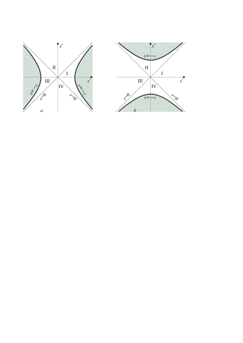
Figure 1: The domain of definition of the Liouville metric for the naked singularity, $\Phi>0$, $c>0$ (a) and the black hole, $\Phi<0$, $c<0$ (b). The forbidden regions of coordinates are filled in grey. Dashed lines correspond to horizons.

In Fig. 1b the allowed region of coordinates is shown for $\Phi<0$ and $c<0$. Test particles moving from light infinities can live forever in the Universe (the rotated quadrants I or III) or fall into the black hole singularity at a finite proper time, the cone $s=0$ being the horizon. This spacetime describes formation of the black hole singularity $s=-c$, $x^{0}>0$ by the scalar field, because the solution is not stationary in quadrants I and III. There is no singularity for $x^{0}<0$ except the white hole in quadrant IV. At a finite proper time the horizon appears, and afterwards the spacelike singularity is formed. Figures 2 and 3 show allowed regions of coordinates in all other cases. Physical meaning of these global solutions is not clear now.

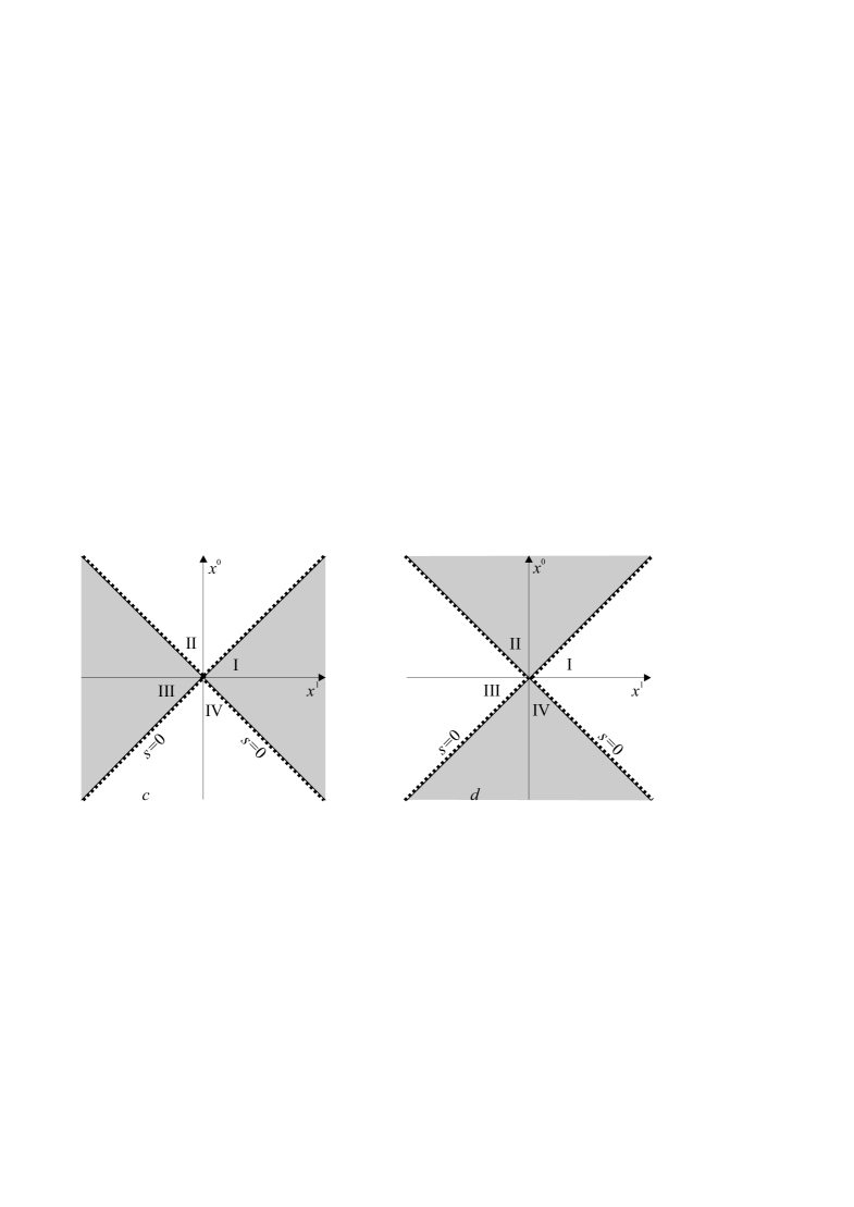
Figure 2: The domain of coordinates definition for two cones with the Liouville metric for $\Phi>0$, $c=0$ (c) and $\Phi<0$, $c=0$ (d).

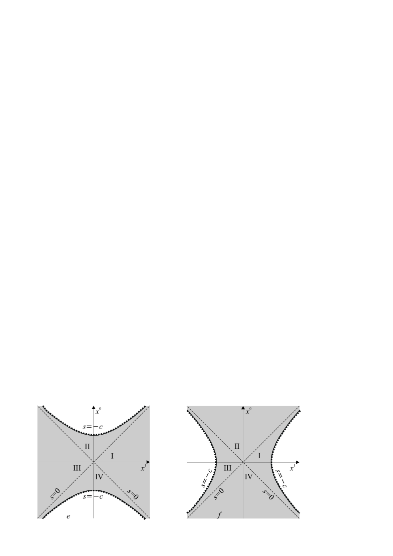
Figure 3: The domain of coordinates definition for two hyperboloids with the Liouville metric for $\Phi>0$, $c<0$ (e) and $\Phi<0$, $c>0$ (f).

3 Friedman-like form of the Liouville metric

The Liouville metric (22) can be written in the Friedmann form by introduction of pseudospherical coordinates in quadrant II rotated in two extra space dimensions:

$$\begin{split}x^{0}:=&t\cosh\chi,\\ x^{1}:=&t\sinh\chi\sin\theta\cos\varphiup,\\ x^{2}:=&t\sinh\chi\sin\theta\sin\varphiup,\\ x^{3}:=&t\sinh\chi\cos\theta,\end{split}$$

where

$$t>0,\qquad\chi\in(0,\infty),\qquad\theta\in(0,\pi),\qquad\varphiup\in(0,2\pi).$$

The rotated quadrant IV is covered by the same coordinates with the replacement $t\mapsto-t$.

In these coordinates $s=t^{2}>0$, and the metric takes the form

$$ds^{2}=(t^{2}+c)\Big{(}dt^{2}-t^{2}d\Omega\Big{)},$$ (27)

where

$$d\Omega:=d\chi^{2}+\sinh^{2}\chi(d\theta^{2}+\sin^{2}\theta d\varphiup^{2})$$

is the metric on the north sheet of two sheeted hyperboloid embedded in Minkowskian spacetime ${\mathbb{R}}^{1,3}$ (constant negative curvature three dimensional Riemannian manifold).

In rotated quadrants I or III, the Liouville metric cannot be written in the Friedmann form because hypersurfaces $s=\text{\sf\small const}$ are timelike. This means that the Friedmann form of metric (22) is accessible only inside the light cone with the vertex at the origin of the coordinate system.

After next coordinate transformation $t=\sqrt{\tilde{t}}$, $\tilde{t}>0$, the Liouville metric becomes

$$ds^{2}=\frac{1}{4}\left(1+\frac{c}{\tilde{t}}\right)d\tilde{t}^{2}-\tilde{t}(\tilde{t}+c)d\Omega.$$ (28)

Its limit $s\to\infty\Leftrightarrow\tilde{t}\to\infty$ differs from the Lorentz metric by factor $1/4$:

$$ds^{2}=\frac{1}{4}d\tilde{t}^{2}-\tilde{t}^{2}d\Omega.$$

It is the Friedmann metric with the scale factor $2\tilde{t}$. One may check that curvature tensor components for this metric differ from zero, but its simplest invariants (24)–(26) vanish at time infinity $\tilde{t}\to\infty$.

The exact metric (27) in quadrant II can be easily rewritten in the Friedmann form too. We introduce new time coordinate $\tau(t)$ defined by the differential equation

$$\frac{d\tau}{dt}=\sqrt{t^{2}+c},\qquad t^{2}+c>0.$$ (29)

Then

$$\tau-\tau_{0}=\frac{t\sqrt{t^{2}+c}}{2}+\frac{c}{2}\text{\sf\small\, ln}\left|t+\sqrt{t^{2}+c}\right|,\qquad\tau_{0}=\text{const}.$$ (30)

The respective metric becomes

$$ds^{2}=d\tau^{2}-a^{2}(\tau)d\Omega,$$ (31)

where the scale factor

$$a(\tau)=t\sqrt{t^{2}+c}$$

is defined implicitly by Eq. (30). Its derivatives are

$$\begin{split}\frac{da}{d\tau}=&\frac{2t^{2}+c}{t^{2}+c},\\ \frac{d^{2}a}{d\tau^{2}}=&\frac{2ct}{(t^{2}+c)^{5/2}}.\end{split}$$ (32)

We see that the Universe in quadrant II is expanding with acceleration, constant velocity and deceleration for $c>0$, $c=0$, and $c<0$, respectively. In quadrant IV the situation is opposite.

Thus, expansion with acceleration takes place only for the naked singularity corresponding to $\Phi>0$ and $c>0$ in quadrant II (see Fig. 1a). This expansion starts from the “horizon”, $t=0$, with zero scale factor, and there is no singularity in global coordinates. Going back in time, homogeneity and isotropy of space sections are lost after crossing the “horizon”, and an observer turns out in the throat of the naked singularity. He sees signals from the naked singularity corresponding to $s=-c$ and a hole in the center. Timelike geodesics can go through this hole and be extended to infinite past. There is no Big Bang in this scenario.

Cases $c=0$ and $c<0$ for positive conformal factor are shown in Figs. 2a and 3a. The singularity at $s=-c$ may be interpreted as the Big Bang but corresponding Universe expands with constant velocity or deceleration, respectively.

Let us compare the Liouville Universe (31) with the Milne metric [15]. For $c=0$, Eq. (29) yields

$$\tau=\frac{1}{2}t^{2}+C_{0},\qquad C_{0}\in{\mathbb{R}}.$$

Putting integration constant to zero, $C_{0}=0$, we get

$$ds^{2}=d\tau^{2}-4\tau^{2}d\Omega.$$ (33)

This expression differs from the Milne metric by factor $4$, which is essential and cannot be removed. The Milne metric is defined on the part of the Minkowskian spacetime and has vanishing curvature. In this sense it is trivial: there is no matter. It describes expanding universe with constant velocity. Its maximal extensions along geodesics lines is the usual flat Minkowskian spacetime. In our case, maximal extension of metric (33) has nonzero curvature and describes only two cones with singular boundary shown in Fig. 2a. Therefore, the Milne metric is essentially different and not contained in expression (22).

If the conformal factor is negative, the solution is defined in quadrant II only in the interior of the black hole solution depicted in Fig. 1b ($\Phi<0$ and $c:=-\lambda^{2}<0$, $\lambda>0$). Then metric (27) becomes

$$ds^{2}=-(\lambda^{2}-t^{2})(dt^{2}-t^{2}d\Omega).$$

The new time variable is defined by the ordinary differential equation

$$\frac{d\tau}{dt}=\sqrt{\lambda^{2}-t^{2}},\qquad t<\lambda.$$

Its general solution is

$$\tau-\tau_{0}=\frac{t\sqrt{\lambda^{2}-t^{2}}}{2}+\frac{\lambda^{2}}{2}\arcsin\left(\frac{t}{\lambda}\right),$$

and the metric takes the Friedmann form

$$ds^{2}=-d\tau^{2}+a^{2}(\tau)d\Omega,$$

where the scale factor is

$$a(\tau)=t\sqrt{\lambda^{2}-t^{2}}.$$

Its derivatives are

$$\begin{split}\frac{da}{d\tau}=&\frac{\lambda^{2}-2t^{2}}{\lambda^{2}-t^{2}},\\ \frac{d^{2}a}{d\tau^{2}}=&-\frac{2\lambda^{2}t}{(\lambda^{2}-t^{2})^{5/2}}.\end{split}$$ (34)

The scale factor is zero both at the horizon, $t=0$, and singularity, $t=\lambda$. For $0<t<\frac{\lambda}{\sqrt{2}}$ and $\frac{\lambda}{\sqrt{2}}<t<\lambda$, space sections in the interior of the black hole expand and contract with deceleration, respectively.

Similar construction can be performed in quadrants I and III. We introduce there pseudospherical coordinates

$$\begin{split}x^{0}:=&r\sinh\chi,\\ x^{1}:=&r\cosh\chi\sin\theta\cos\varphiup,\\ x^{2}:=&r\sinh\chi\sin\theta\sin\varphiup,\\ x^{3}:=&r\sinh\chi\cos\theta,\end{split}$$ (35)

where $r>0$ is the spacelike coordinate. They cover the whole one-sheeted hyperboloid obtained by rotation of quadrant I or III in two extra space dimensions. In these coordinates, $s=-r^{2}$, and the Liouville metric becomes

$$ds^{2}=(c-r^{2})(-dr^{2}+r^{2}d\Omega),$$ (36)

where

$$d\Omega:=d\chi^{2}-\cosh^{2}\chi\big{(}d\theta^{2}+\sin^{2}\!\theta d\varphiup^{2}\big{)},$$

the variable $\chi$ playing the role of time. The quadratic form $d\Omega$ is the Lorentzian metric of constant curvature on the one sheeted hyperboloid. In case $c=l^{2}>0$, $l>0$ (naked singularity), we introduce new space coordinate $\rho$ by the differential equation

$$\frac{d\rho}{dr}=\sqrt{l^{2}-r^{2}},\qquad r<l.$$

Its general solution is

$$\rho-\rho_{0}=\frac{r\sqrt{l^{2}-r^{2}}}{2}+\frac{l^{2}}{2}\arcsin\left(\frac{r}{l}\right),\qquad\rho_{0}=\text{\sf\small const}.$$

Now the Liouville metric is

$$ds^{2}=-d\rho^{2}+r^{2}(l^{2}-r^{2})\big{[}d\chi^{2}-\cosh^{2}\!\chi(d\theta^{2}+\sin^{2}\!\theta d\varphiup^{2})\big{]}.$$ (37)

It is not in Friedmann-like form, because the time coordinate is $\chi$. Note that the Liouville metric cannot be brought into the Friedmann form in quadrant I or III because any spacelike section does not evolve.

4 Geodesics for the Liouville spacetime

We analyze geodesic lines for metric (22) using the Hamilton–Jacobi technique. The Lagrangian and Hamiltonian for timelike geodesics $\big{(}x^{\alpha}(\tau)\big{)}$ and metric signature $(+---)$ are:

$$L= \frac{1}{2}(s+c)\eta_{\alpha\beta}\dot{x}^{\alpha}\dot{x}^{\beta},$$ (38)

$$H= \frac{1}{2(s+c)}\eta^{\alpha\beta}p_{\alpha}p_{\beta},\qquad p_{\alpha}=(s+c)\eta_{\alpha\beta}\dot{x}^{\beta},$$ (39)

where the dot denotes derivative with respect to canonical parameter $\tau\in{\mathbb{R}}$. Geodesic Hamiltonian equations have the form

$$\begin{split}\dot{x}^{\alpha}=&\frac{1}{s+c}p^{\alpha},\\ \dot{p}_{\alpha}=&\frac{p_{\beta}p^{\beta}}{(s+c)^{2}}x_{\alpha},\end{split}$$ (40)

where $p^{\alpha}:=\eta^{\alpha\beta}p_{\beta}$ and $x_{\alpha}:=\eta_{\alpha\beta}x^{\beta}$. Sure, they are equivalent to geodesic equations in the Lagrangian formulation

$$\ddot{x}^{\alpha}=-\Gamma_{\beta\gamma}{}^{\alpha}\dot{x}^{\beta}\dot{x}^{g}=\frac{1}{s+c}(x^{\alpha}\dot{x}_{\beta}\dot{x}^{\beta}-2x_{\beta}\dot{x}^{\beta}\dot{x}^{\alpha}).$$ (41)

These equations are clearly invariant with respect to reflection of each coordinate $x^{\alpha}\rightarrow-x^{\alpha}$ separately.

Equations (41) can be integrated using the Hamilton–Jacobi technique. The Hamilton–Jacobi equation for the action function $W(x)$ is (see, i.e. [16])

$$\frac{1}{s+c}\eta^{\alpha\beta}\partial_{\alpha}W\partial_{\beta}W=2m^{2},\qquad s+c\neq 0,$$ (42)

where $m>0$ is the mass of a test particle moving in the spacetime. The complete integral of Eq. (42) depends on four independent parameters $d=(d_{\alpha})\in{\mathbb{R}}^{4}$. The Hamilton–Jacobi equation admits complete separation of variables, by definition, if a complete integral has the form (see, e.g. [13])

$$W(x,d)=\sum_{\alpha=0}^{3}W_{\alpha}(x^{\alpha},d),\qquad\text{\sf\,\small\, det\,}\frac{\partial^{2}W}{\partial x^{\alpha}\partial d_{\beta}}\neq 0,$$

where each summand depends only on single coordinate and, possibly, a full set of independent parameters $d$. In this case, variables in Eq. (42) are completely separated as

$$W^{\prime 2}_{\alpha}=2m^{2}x_{\alpha}^{2}+d_{\alpha},\qquad\forall\alpha,$$ (43)

where $W^{\prime}_{\alpha}:=\partial_{\alpha}W_{\alpha}$ and $d_{0}-d_{1}-d_{2}-d_{3}=2m^{2}c$. We can choose, for example, $d_{1},d_{2},d_{3},2m^{2}$ as the full set of independent parameters in the complete integral of the Hamilton–Jacobi equation (42).

The above consideration concerns metric of signature $(+---)$ and only timelike geodesics. If the right hand side of the Hamilton–Jacobi equation (42) is replaced by $0$ and $-2m^{2}$, then it describes lightlike (null) and spacelike geodesics, respectively. For metric signature $(-+++)$ the situation is opposite: $-2m^{2}$, $0$, and $2m^{2}$ correspond to timelike, null, and spacelike geodesics. Therefore, geodesics for signature $(-+++)$ are obtained from these for signature $(+---)$ by simple rotation of pictures on $x^{0},x^{i}$ plain by angle $\pi/2$.

We can always put $2m^{2}=1$, $m>0$, by stretching the canonical parameter in all cases. This means that the length of timelike and spacelike geodesics is chosen as the canonical parameter.

4.1 Lightlike (null) geodesics

The Hamilton–Jacobi equation (42) for lightlike (null) geodesics, which are the simplest ones, takes the form

$$\eta^{\alpha\beta}\partial_{\alpha}W\partial_{\beta}W=0$$

for both signatures $s+c>0$ and $s+c<0$. Timelike geodesics must satisfy the constraint $\dot{x}^{\alpha}\dot{x}_{\alpha}=0$, which is equivalent to $p_{\alpha}p^{\alpha}=0$ due to Eq. (39). Therefore, the complete integral of the Hamilton–Jacobi equation is

$$W=\sum_{\alpha=0}^{3}W_{\alpha},$$

where separating functions are defined by ordinary differential equations

$$W_{\alpha}^{\prime 2}=d_{\alpha},\qquad d_{0}-d_{1}-d_{2}-d_{3}=0.$$ (44)

Obviously, all parameters must be positive, and, therefore, we denote them by $d_{\alpha}:=k_{\alpha}^{2}$, $k_{0}>0$, $k_{i}\geq 0$, $i=1,2,3$. Separating functions for null geodesics are linear

$$W_{\alpha}=k_{\alpha}x^{\alpha}+\tilde{b}_{\alpha},\qquad\text{(no summation)},$$

where $\tilde{b}_{\alpha}\in{\mathbb{R}}$ are integration constants.

In the Hamiltonian formulation, there are four involutive conservation laws (all momenta are conserved):

$$p_{\alpha}=k_{\alpha}.$$

They are linear but not quadratic because square root of Eq. (44) can be taken. Using definition of momenta (39), conservation laws can be rewritten as differential equations for coordinates:

$$(s+c)\dot{x}^{\alpha}=k^{\alpha},\qquad k^{\alpha}:=\eta^{\alpha\beta}k_{\beta},\qquad\forall\alpha.$$ (45)

Rescaling the canonical parameter, we can put $k^{0}=1$ without loss of generality. Dividing these relations, we obtain equations for the form of geodesic lines

$$\frac{dx^{i}}{dx^{0}}=k^{i},\qquad i=1,2,3.$$

They are easily integrated

$$x^{i}=k^{i}x^{0}+b^{i},$$ (46)

where $b^{i}\in{\mathbb{R}}$ are integration constants. We see that all null geodesics are straight lines going through each point of the space-time in direction of the null vector $(k^{0}=1,k^{i})$, i.e. they cross a plane $x^{0}=\text{\sf\small const}$ by angle $\pi/4$. This means that null geodesics have the same form as in the Minkowskian spacetime, as expected. The difference is related to the dependence on the canonical parameter.

To find this dependence, we have to solve, for example, Eq. (45) for $\alpha=0$. Equation (46) implies

$$s=2kx^{0}+b,\qquad k:=-\delta_{ij}k^{i}b^{j},\quad b:=-\delta_{ij}b^{i}b^{j}\leq 0.$$ (47)

Then we obtain dependence on the canonical parameter

$$(2kx^{0}+b+c)\dot{x}^{0}=1\qquad\Leftrightarrow\qquad\tau-\tau_{0}=k\big{(}x^{0}\big{)}^{2}+(b+c)x^{0},$$ (48)

where $\tau_{0}$ is an integration constant, which can be put to zero. We see that every point with finite $x^{0}$ is reached by null geodesic at a finite value of the canonical parameter. It means, in particular, that all singular points are incomplete with respect to null geodesics. Null geodesics go to lightlike infinity only when $x^{0}\to\pm\infty$. The second equality (48) implies that $\tau\to\pm\infty$ when $x^{0}\to\pm\infty$ for $k\neq 0$. If $k=0$ and $b+c=0$, then $s+c=0$ due to Eq. (47), which is forbidden. Therefore, lightlike infinities are geodesically complete, but singularities are not.

4.2 Timelike geodesics for $\Phi>0$

If metric has signature $(+---)$ corresponding to positive conformal factor $\Phi=s+c>0$, then the right hand side of the Hamilton–Jacobi equation (42) is equal to $2m^{2}$ and $-2m^{2}$ for timelike and spacelike geodesics, respectively. For inverse signature $(-+++)$, $s+c<0$, the situation is opposite: the right hand side is $-2m^{2}$ and $2m^{2}$ for timelike and spacelike geodesics. Without loss of generality, we put $2m^{2}=1$ by rescaling the canonical parameter in all cases for simplicity.

First, we consider timelike geodesics for signature $(+---)$. Separating functions $W_{\alpha}$ in this case are defined by ordinary differential equations:

$$W_{\alpha}^{\prime 2}=\big{(}x^{\alpha}\big{)}^{2}+d_{\alpha}>0,\qquad\forall\alpha,$$ (49)

where

$$d_{0}-d_{1}-d_{2}-d_{3}=c.$$ (50)

In this way, variables in the Hamilton–Jacobi equation (42) are completely separated, and hence the Liouville metric belongs to class $[0,4,0]_{2}$ of separable metrics according to the classification given in [13].

In the Hamiltonian formulation, equations for separating functions (49) correspond to four involutive quadratic conservation laws:

$$(p_{\alpha})^{2}-\big{(}x^{\alpha}\big{)}^{2}=d_{\alpha}$$

corresponding to four Killing second rank tensors. Sure, we have to require $\big{(}x^{\alpha}\big{)}^{2}+d_{\alpha}>0$ for all $\alpha$, which restrict the range of coordinates for given parameters $d_{\alpha}$. To find geodesic lines, we integrate further the respective equations for coordinates:

$$(s+c)^{2}\big{(}\dot{x}^{\alpha}\big{)}^{2}=\big{(}x^{\alpha}\big{)}^{2}+d_{\alpha}.$$ (51)

It is easily checked that the velocity of all geodesics equals unity:

$$g_{\alpha\beta}\dot{x}^{\alpha}\dot{x}^{\beta}=1,$$

as it should be.

Equations (51) have singular solutions corresponding to particles resting at points

$$x^{i}=\pm\sqrt{-d_{i}},\qquad\forall d_{i}\leq 0.$$ (52)

For these particles, the conformal factor must be positive: $s+c=\big{(}x^{0}\big{)}^{2}+d_{0}>0$, the dependance on time being given by differential equation following from Eq. (51):

$$\big{[}\big{(}x^{0}\big{)}^{2}+d_{0}\big{]}\big{(}\dot{x}^{0}\big{)}^{2}=1.$$

Choosing orientation of the canonical parameter $\dot{x}^{0}>0$, we get a general solution

$$\tau-\tau_{0}=\frac{x^{0}\sqrt{\big{(}x^{0}\big{)}^{2}+d_{0}}}{2}+\frac{d_{0}}{2}\text{\sf\small\, ln}\left|x^{0}+\sqrt{\big{(}x^{0}\big{)}^{2}+d_{0}}\right|,$$

where $\tau_{0}$ is an integration constant and $d_{0}=c+d_{1}+d_{2}+d_{3}$. This solution is defined for all $x^{0}\in{\mathbb{R}}$ if $d_{0}\geq 0$. For $d_{0}<0$, the solution exists if $\big{(}x^{0}\big{)}^{2}>|d_{0}|$, where boundary points $x_{0}=\pm\sqrt{-d_{0}}$ correspond to singularity $s+c=0$.

Singular solutions (52) satisfy original geodesic equations (41) for $\alpha=0$. However, for space indices $\alpha=i$ we obtain nontrivial relations

$$\frac{x^{i}}{\Big{(}\big{(}x^{0}\big{)}^{2}+d_{0}\Big{)}^{2}}=0.$$

It means that singular solutions (52) are not geodesics unless all $d_{i}=0\Leftrightarrow x^{i}=0$. Only the symmetry axis $x^{0}$ for $d_{0}=c$ and $x^{i}=0$ is the geodesic line.

The form of general type geodesics is defined by equation

$$\left(\frac{dx^{i}}{dx^{0}}\right)^{2}=\frac{\big{(}x^{i}\big{)}^{2}+d_{i}}{\big{(}x^{0}\big{)}^{2}+d_{0}},\qquad i=1,2,3,$$ (53)

obtained by dividing equations (51). Inequality

$$\big{(}x^{0}\big{)}^{2}+d_{0}=s+c+\big{(}x^{1}\big{)}^{2}+d_{1}+\big{(}x^{2}\big{)}^{2}+d_{2}+\big{(}x^{3}\big{)}^{2}+d_{3}>\big{(}x^{i}\big{)}^{2}+d_{i},\qquad\forall i,$$

implies that the right hand side of Eq.(53) is less then unity, i.e. the geodesic tangent vector lies inside light cones as it should be. Equation (53) is equivalent to two equations:

$$\pm\frac{dx^{i}}{\sqrt{\big{(}x^{i}\big{)}^{2}+d_{i}}}=\frac{dx^{0}}{\sqrt{\big{(}x^{0}\big{)}^{2}+d_{0}}}.$$ (54)

Their general solution is

$$\left|x^{i}\pm\sqrt{\big{(}x^{i}\big{)}^{2}+d_{i}}\right|=C^{i}\left|x^{0}+\sqrt{\big{(}x^{0}\big{)}^{2}+d_{0}}\right|,$$ (55)

where $C^{i}>0$ is an integration constant and $d_{\alpha}\neq 0$ for all $\alpha$. Modulus signs can be dropped assuming that integration constants may have any sign. Parameters $(d_{\alpha})$ can be arbitrary with the only constraint (50), and the range of coordinates is restricted by inequalities $\big{(}x^{\alpha}\big{)}^{2}+d_{\alpha}>0$.

General solution (55) without module signs can be rewritten as

$$\sqrt{\big{(}x^{0}\big{)}^{2}+d_{0}}=-x^{0}+\frac{1}{C^{i}}\left(x^{i}\pm\sqrt{\big{(}x^{i}\big{)}^{2}+d_{i}}\right).$$

The square of this equation yields

$$\begin{split}x^{0}=&\frac{1}{2C^{i}}\left(x^{i}\pm\sqrt{\big{(}x^{i}\big{)}^{2}+d_{i}}\right)-\frac{C^{i}d_{0}}{2\left(x^{i}\pm\sqrt{\big{(}x^{i}\big{)}^{2}+d_{i}}\right)}=\\ &=\left(\frac{1}{2C^{i}}+\frac{C^{i}d_{0}}{2d_{i}}\right)x^{i}\pm\left(\frac{1}{2C^{i}}-\frac{C^{i}d_{0}}{2d_{i}}\right)\sqrt{\big{(}x^{i}\big{)}^{2}+d_{i}}.\end{split}$$ (56)

In a similar way, it can be rewritten in equivalent form without $\pm$ sign

$$x^{i}=\left(\frac{C^{i}}{2}+\frac{d_{i}}{2C^{i}d_{0}}\right)x^{0}+\left(\frac{C^{i}}{2}-\frac{d_{i}}{2C^{i}d_{0}}\right)\sqrt{\big{(}x^{0}\big{)}^{2}+d_{0}}.$$ (57)

The $\pm$ sign in Eq. (56) tells us that there may be two points for given $x^{i}$. Equation (57) proves that every general geodesic is infinitely smooth in their domains of definitions.

There are three degenerate cases, which should be considered separately. The first one corresponds to $d_{0}=0$ and $d_{i}\neq 0$. Then Eq. (54) is equivalent to relations

$$\pm\frac{dx^{i}}{\sqrt{\big{(}x^{i}\big{)}^{2}+d_{i}}}=\frac{dx^{0}}{x^{0}},$$

which has a general solution

$$x^{0}=\frac{x^{i}\pm\sqrt{\big{(}x^{i}\big{)}^{2}+d_{i}}}{C^{i}},$$ (58)

where $C^{i}\neq 0$ is an integration constant. It can be rewritten without $\pm$ sign

$$x^{i}=\frac{\big{(}C^{i}x^{0}\big{)}^{2}-d_{i}}{2C^{i}x^{0}}.$$ (59)

In the second degenerate case $d_{0}\neq 0$ and $d_{i}=0$. The general solution of Eq. (54) is

$$x^{i}=\frac{x^{0}\pm\sqrt{\big{(}x^{0}\big{)}^{2}-d_{0}}}{C^{0}},$$ (60)

where $C^{0}\neq 0$ is an integration constant. It is rewritten as

$$x^{0}=\frac{\big{(}C^{0}x^{i}\big{)}^{2}-d_{0}}{2C^{0}x^{i}}.$$ (61)

The third degenerate case appears when $d_{0}=0$ and $d_{i}=0$. Then Eq. (54) has a general solution

$$x^{0}=C^{i}x^{i},\qquad\text{and}\qquad x^{0}=\frac{C^{i}}{x^{i}},\qquad C^{i}\neq 0,\qquad\text{(no summation)}.$$ (62)

This solution corresponds to special values of parameters. For example, if $d_{0}=0$ and $d_{1}=0$, then the remaining parameters must satisfy relation $-d_{2}-d_{3}=1$.

Before drawing typical timelike geodesics, we resolve modulus signs in Eqs. (55) and analyse functions

$$f_{\pm}(x):=x\pm\sqrt{x^{2}+d}.$$

Function $f_{+}$ is drawn in Fig. 4a, for different values of $d$. It is positive for all $d$ and $x\geq 0$ and consists of two branches for negative $d<0$ and $x\leq-\sqrt{-d}$. Its asymptotics are

$$f_{+}(x)\approx ~{}2x+\frac{d}{2x}, x\to\infty,$$

$$f_{+}(x)\approx -\frac{d}{2x}, x\to-\infty,$$

$$f_{+}(x)\approx ~{}\sqrt{d}+x+\frac{x^{2}}{2\sqrt{d}}, x\to 0, d>0,$$

$$f_{+}(x)\approx ~{}\sqrt{-d}\left(1+\epsilon+\!\sqrt{2\epsilon}\right), \epsilon\to 0_{+}, d<0, x:= \sqrt{-d}\left(1+\epsilon\right),$$

$$f_{+}(x)\approx -\!\sqrt{-d}\left(1+\epsilon-\!\sqrt{2\epsilon}\right), \epsilon\to 0_{+}, d<0, x:= -\!\sqrt{-d}\left(1+\epsilon\right).$$

It is clear that $f_{-}=-f_{+}(-x)$.

Let us consider geodesics of general type in the $x^{1}$, $x^{0}$ plane for simplicity. These geodesics exist only for $d_{2,3}=0$ and $x^{2,3}=0$ due to Eq. (51). Null geodesics in the $x^{0}$, $x^{1}$ plane are $x^{0}=\pm x^{1}+\text{\sf\small const}$. So, light cones are the same as in the Minkowskian plane. Equation (55) on the $x^{0},x^{1}$ plane is equivalent to equation

$$x^{0}=\left(\frac{1}{2C^{1}}+\frac{(c+d_{1})C^{1}}{2d_{1}}\right)x^{1}\pm\left(\frac{1}{2C^{1}}-\frac{(c+d_{1})C^{1}}{2d_{1}}\right)\sqrt{\big{(}x^{1}\big{)}^{2}+d_{1}}.$$ (63)

where $d_{1}\neq 0$ and $d_{0}=c+d_{1}\neq 0$. Thus, we obtained a general solution of the geodesic equations on the $x^{0},x^{1}$ plain depending on two integration constants $C^{1}\neq 0$ and $d_{1}$. Note that for

$$d_{1}=\frac{c\big{(}C^{1}\big{)}^{2}}{1-\big{(}C^{1}\big{)}^{2}}$$

the general type geodesic is a straight line $x^{0}=x^{1}/C^{1}$.

Timelike geodesics of general type for the naked singularity in Fig. 1a, $c=1$, $C^{1}=1/2$, and different positive $d_{1}>0$ are shown in Fig. 4b. For $d_{1}=1/3$ the geodesic is the straight line. Sure, one has to add geodesics obtained by reflection of space coordinate $x^{1}\to-x^{1}$ due to the $\pm$ sign in Eq. (54).

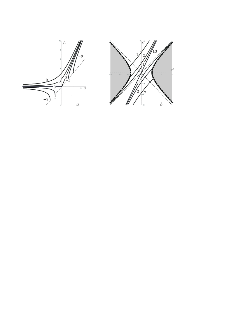
Figure 4: Function $f_{+}(x)$ for different values of parameter $d$, (a). Timelike geodesics for the naked singularity, $c=1$, $C^{1}=1/2$, and positive $d_{1}>0$ (b). The numbers denote the values of parameter $d_{1}$ on both pictures.

Timelike geodesics for $c=1$ and negative $d_{1}<0$ are drawn in Fig, 5. Fig. 5a shows general type geodesics for $C^{1}=1/2$ and different values of $d_{1}<0$, the numbers denoting the values of $d_{1}$. They are obtained by gluing two branches from Fig. 5a at the points where they touch singular solutions. The latter are vertical lines in Fig. 5b enveloping general type geodesics of the same $d_{1}$ but different values of $C^{1}$.

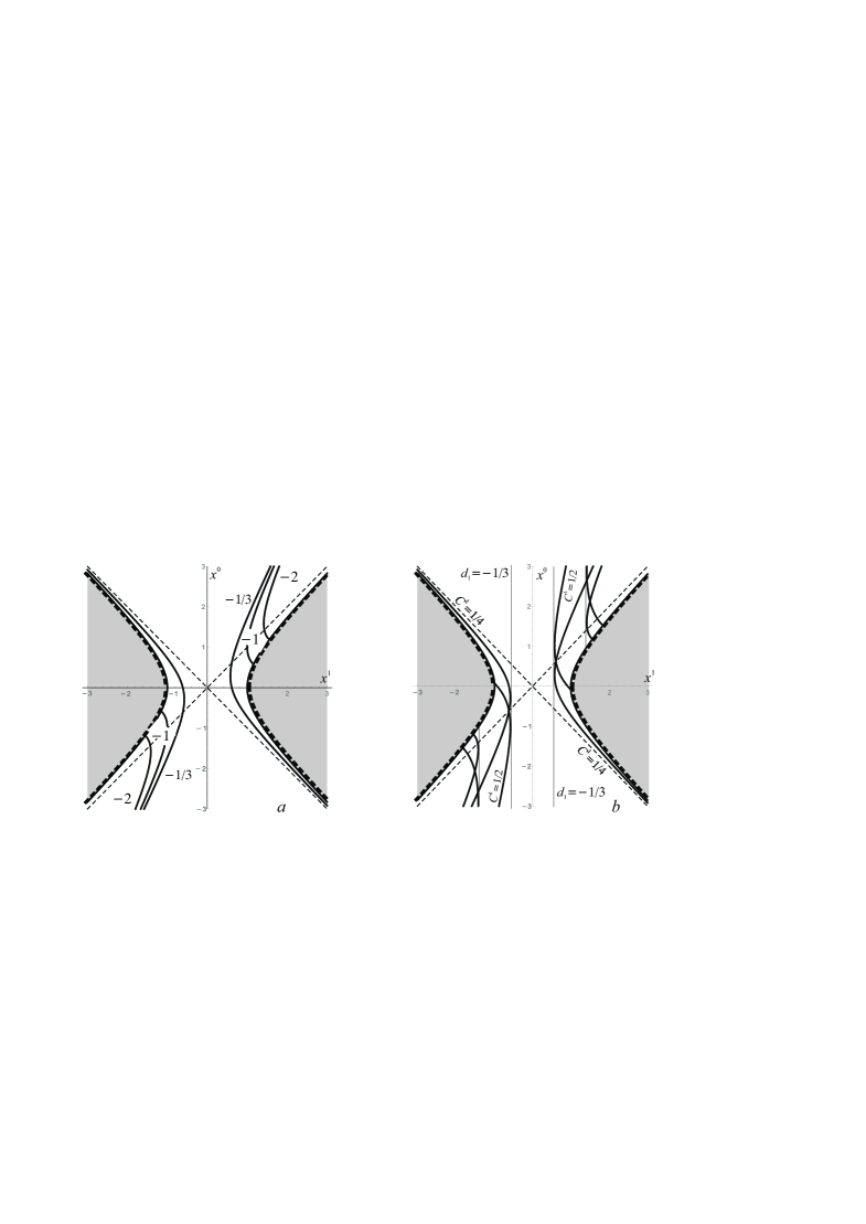
Figure 5: Timelike general type geodesics for the naked singularity, $c=1$, $C^{1}=1/2$, and different negative values of $d_{1}<0$ (a). General type geodesics with the same parameter $d_{1}$ but different $C^{1}$ touch the singular solution which is the vertical line in Fig. b.

There are also degenerate geodesics of general type. Let $d_{0}=0$, then $d_{1}=-c$, and general solution of Eq. (54) becomes

$$x^{0}=\frac{x^{1}\pm\sqrt{\big{(}x^{1}\big{)}^{2}-c}}{C^{1}},$$ (64)

where $C^{1}\neq 0$ is an integration constant. These degenerate geodesics smoothly touch at points $\big{(}x^{0}=\sqrt{c}/C^{1},x^{1}=\sqrt{c}\big{)}$ singular straight solutions $x^{1}=\pm c$ going through vertices of hyperbolas $\big{(}x^{0}\big{)}^{2}-\big{(}x^{1}\big{)}^{2}=c$. Equation (64) with $+$ and $-$ signs describes the upper and lower parts of the degenerate geodesic in Fig. 6a on the right.

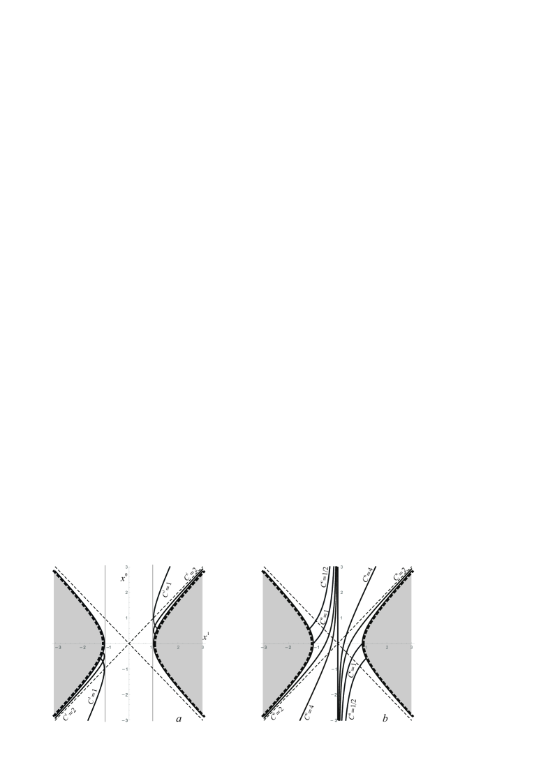
Figure 6: Timelike degenerate geodesics of general type for the naked singularity, $c=1$, $d_{0}=0$, and $d_{1}=-c$. They touch singular solutions $x^{1}=\pm c$ for different values of $C^{1}$ (a). Timelike degenerate type geodesics for $c=1$, $d_{0}=c$, $d_{1}=0$, and different values of $C^{0}$. They touch the singular geodesic $x^{1}=0$ at infinities $x^{0}=\pm 1$.

The second degenerate case corresponds to $d_{0}=c$ and $d_{1}=0$. Now a general solution of Eq. (54) is

$$x^{1}=\frac{x^{0}\pm\sqrt{\big{(}x^{0}\big{)}^{2}+c}}{C^{0}},$$

where $C^{0}\neq 0$ is an integration constant. It can be rewritten as

$$x^{0}=\frac{\big{(}x^{1}C^{0}\big{)}^{2}-c}{2x^{1}C^{0}}.$$ (65)

These geodesics are shown in Fig. 6b for $c=1$ and different values of $C_{0}$. They touch the singular geodesic $x^{1}=0$ at infinities $x^{0}=\pm\infty$.

There are no third degenerate timelike geodesics on the $x^{0}$, $x^{1}$ plain because $d_{0}=d_{1}=d_{2}=d_{3}=0$ in this case, which contradicts assumption (50).

We see that first integrals of geodesic equations admit singular solutions which are not geodesics except symmetry axis $x^{0}$. In spite of their existence, one and only one timelike geodesic goes through every point of spacetime in a given direction.

Now we consider timelike geodesics for the space-time with $\Phi>0$, $c=0$ depicted in Fig. 7a. Singular solutions are the same as in the previous case (52) and exist only for nonpositive $d_{i}\leq 0$. Timelike geodesics of general type are given by Eqs. (55), (58), and (60), the only difference being the relation between parameters $d_{0}-d_{1}-d_{2}-d_{3}=0$. Timelike geodesics of general type on the $x^{0}$, $x^{1}$ plain are given by Eq. (63) with $c=0$, which can be rewritten as

$$x^{0}=\frac{1}{2}\left(\frac{1}{C^{1}}+C^{1}\right)x^{1}\pm\frac{1}{2}\left(\frac{1}{C^{1}}-C^{1}\right)\sqrt{\big{(}x^{1}\big{)}^{2}+d_{1}},$$ (66)

where $C^{1}\neq 0$. Fig. 7a shows several geodesics of general type for positive $d_{1}>0$.

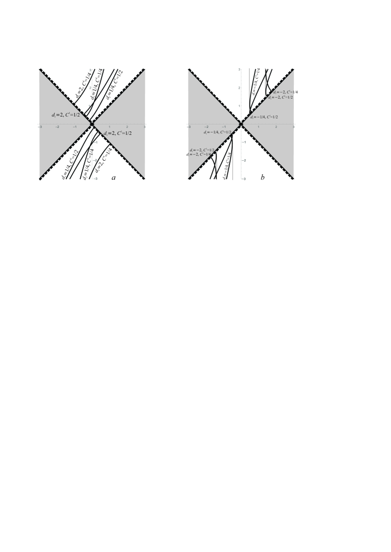
Figure 7: Timelike general type geodesics for two cones, $\Phi>0$, $c=0$, for different $d_{1}$ and $C^{1}$ (a). Two general type geodesics with the same negative $d_{1}<0$ touch singular geodesics (vertical lines) (b).

General type geodesics with the same negative $d_{1}<0$ but different $C^{1}$ touch singular vertical geodesics $x^{1}=\pm\sqrt{-d_{1}}$ in Fig. 7b.

There are also degenerate geodesics of general type corresponding to $d_{0}=d_{1}=0$:

$$x^{0}=\frac{x^{1}}{C^{1}},\qquad\big{|}C^{1}\big{|}>1,$$

and

$$x^{0}=\frac{\tilde{C}^{1}}{x^{1}},\qquad\big{(}x^{1}\big{)}^{2}\leq\big{|}\tilde{C}^{1}\big{|},$$

where inequalities follow from the requirement $\Phi>0$. They are drawn in Fig. 8a for different integration constants. Degenerate geodesics with integration constant $C^{1}$ are straight lines going through the origin. The geodesics with $\tilde{C}^{1}$ are hyperbolas touching singular geodesic $x^{1}=0$ at infinity.

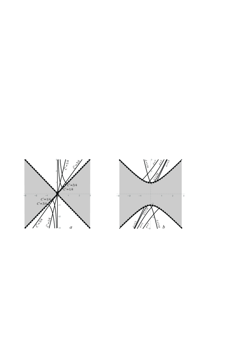
Figure 8: Timelike degenerate geodesics of general type for two cones, $\Phi>0$, $c=0$, for different $C^{1}$ and $\tilde{C}^{1}$ (a). General type geodesics with the same negative $d_{1}<0$ touch singular solutions (vertical lines) (b).

Next we consider timelike geodesics for two hyperboloids $\Phi>0$ and $c<0$ pictured in Fig. 3a. Geodesics of general type for $d_{0}=c+d_{1}\neq 0$, $d_{1}\neq 0$ on the $x^{0},x^{1}$ plain have the form (63) as for the naked singularity. They are drawn in Fig. 8b for $C^{1}=1/2$ and different positive values of $d_{1}$. Geodesics of general type for $C^{1}=1/2$ and different negative values of $d_{1}$ are shown in Fig. 9a.

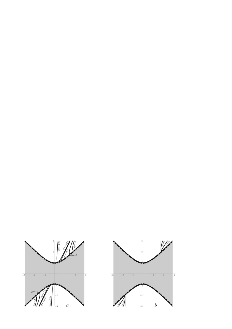
Figure 9: Timelike geodesics of general type for two hyperboloids $\Phi>0$ and $c=-1$ for $C^{1}=1/2$ and different negative $d_{1}<0$ (a). General type geodesics with the same negative $d_{1}=-3$ and different $C^{1}$ touch singular solutions $x^{1}=\pm\sqrt{3}$ (b).

General type geodesics with the same negative $d_{1}$ touch the singular solution $x^{1}=\pm\sqrt{-d_{1}}$ in Fig. 9b.

Degenerate geodesics of the first kind in the spacetime $\Phi>0$, $c=-1$ on the $x^{0}$, $x^{1}$ plain correspond to $d_{0}=0$ and $d_{1}=-c$. They are shown in Fig. 10a for different $C^{1}$.

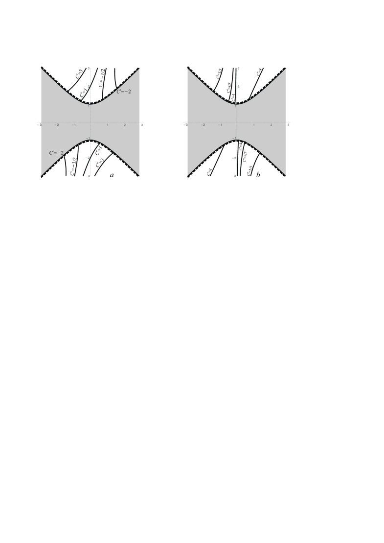
Figure 10: Timelike geodesics of general type for two hyperboloids with $\Phi>0$ and $c=-1$ for $C^{1}=1/2$ and different negative $d_{1}<0$ (a). General type geodesics with the same negative $d_{1}=-3$ and different $C^{1}$ touch singular solutions $x^{1}=\pm\sqrt{3}$ (b).

Degenerate geodesics of the second kind (61) correspond to $d_{0}=c$ and $d_{1}=0$. They are shown in Fig. 10b.

4.3 Spacelike geodesics for $\Phi>0$

The Hamilton–Jacobi equation for spacelike geodesics $x^{\alpha}(\tau)$ for metric signature $(+---)$ is

$$\eta^{\alpha\beta}\partial_{\alpha}W\partial_{\beta}W=-(s+c).$$ (67)

The variables are completely separated by

$$W^{\prime 2}_{\alpha}=-\big{[}\big{(}x^{\alpha}\big{)}^{2}+d_{\alpha}\big{]}\geq 0,$$ (68)

where parameters satisfy previous constraint (50) and must be nonpositive, $d_{\alpha}\leq 0$. Now coordinates vary in the finite region $\big{(}x^{\alpha}\big{)}^{2}\leq-d_{\alpha}$.

Equations (68) yield first integrals for geodesic equations

$$(s+c)^{2}\big{(}\dot{x}^{\alpha}\big{)}^{2}=-\big{(}x^{\alpha}\big{)}^{2}-d_{\alpha}.$$ (69)

They have singular spacelike solution

$$x^{0}=\pm\sqrt{-d_{0}}^{2},$$

$$\big{(}\delta_{jk}x^{j}x^{k}+d_{1}+d_{2}+d_{3}\big{)}^{2}\big{(}\dot{x}^{i}\big{)}^{2}=-\big{(}x^{i}\big{)}^{2}-d_{i}.$$ (70)

Substitution of these expressions into geodesic equations (41) for $\alpha=0$ yields

$$0=-\frac{\sqrt{-d_{0}}}{(s+c)^{2}}.$$

This is a contradictory relation except $d_{0}=0$. It is easily verified that geodesic equations for space indices $\alpha=i$ are satisfied. So, there are singular geodesics only for $d_{0}=0$ which implies $x^{0}=0$, the space coordinates being defined by Eqs. (70).

The form of spacelike and timelike geodesics of general type is defined by the same Eqs. (53) but different signs of $\big{(}x^{\alpha}\big{)}^{2}+d_{\alpha}$. These equations do not admit degenerate spacelike geodesics of general type because equality $d_{\alpha}=0$ implies $x^{\alpha}=0$ due to Eq. (68). Equations (53) for spacelike geodesics can be rewritten in the form

$$\pm\frac{dx^{i}}{\sqrt{-\big{(}x^{i}\big{)}^{2}-d_{i}}}=\frac{dx^{0}}{\sqrt{-\big{(}x^{0}\big{)}^{2}-d_{0}}},\qquad d_{\alpha}\neq 0.$$

A general solution of these equations has the form

$$x^{0}=\sqrt{\frac{d_{0}}{d_{i}}}\left(\pm x^{i}\cos C^{i}+\sqrt{-d_{i}-\big{(}x^{i}\big{)}^{2}}\,\sin C^{i}\right),$$ (71)

where $C^{i}\in{\mathbb{R}}$ is an integration constant. Equation

$$-d_{0}-\big{(}x^{0}\big{)}^{2}=-\frac{d_{0}}{d_{i}}\left[d_{i}\cos^{2}C^{i}+\big{(}x^{i}\big{)}^{2}\cos(2C^{i})\pm x^{i}\sqrt{-d_{i}-\big{(}x^{i}\big{)}^{2}}\,\sin(2C^{i})\right],$$

is useful for verification of the solution.

There are straight spacelike geodesics if $C^{i}=0$ going through the origin of coordinate system

$$x^{0}=\pm\sqrt{\frac{d_{0}}{d_{i}}}\,x^{i}.$$

They exist only for the naked singularity and include singular geodesic for $d_{0}=0$.

To visualize geodesics, we consider them on the $x^{0},x^{1}$ plain. These geodesics corresponding to $d_{2}=d_{3}=0$ and $d_{0}-d_{1}=c$ and zero angular momentum are defined by equation

$$x^{0}=\sqrt{\frac{c+d_{1}}{d_{1}}}\left(\pm x^{1}\cos C^{1}+\sqrt{-d_{1}-\big{(}x^{1}\big{)}^{2}}\,\sin C^{1}\right),$$ (72)

where coordinates are restricted by inequality $\Phi>0$. They become parts of ellipses for $\cos C_{1}=0$. Figs. 11 and 12 show typical spacelike geodesics of general type for naked singularity $(c=1)$, two cones $(c=0)$, and two hyperboloids $(c=-1)$ for different values of $d_{1}$ and $C^{1}$. Sure, there are also reflected geodesics $x^{1}\to-x^{1}$.

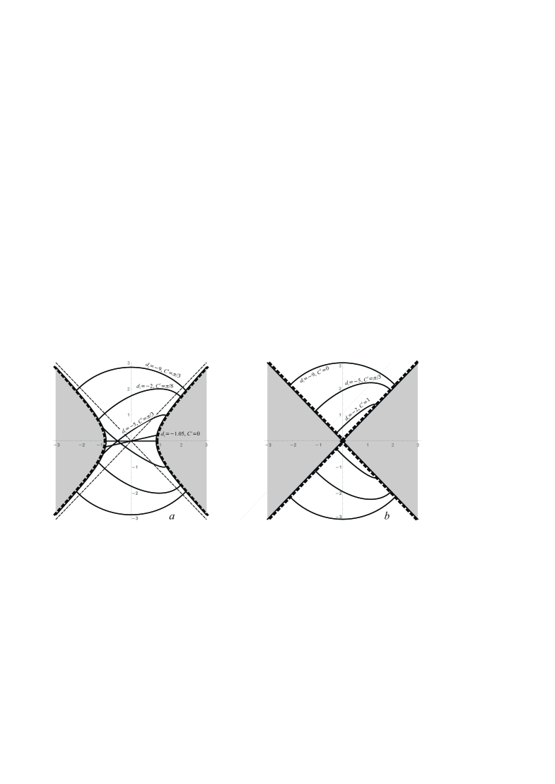
Figure 11: Spacelike geodesics of general type for the naked singularity $c=-1$ (a) and two cones (b) for different values of $C^{1}$ and $d_{1}<0$.

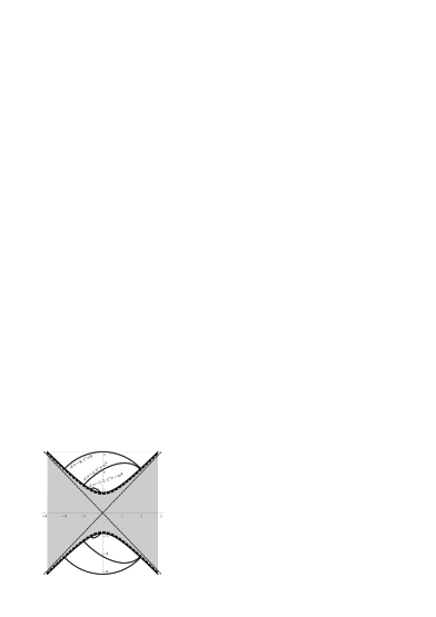
Figure 12: Spacelike geodesics of general type for two hyperboloids for different values of $C^{1}$ and $d_{1}<0$.

4.4 Completeness of geodesics

Solutions in a gravity model are global ones, by definition, if every geodesic can be either extended to infinite value of the canonical parameter or ends up at its finite value at a singular point, where one of geometric invariants becomes infinite. In section 4.1, we analysed completeness of null geodesics, and it was proved that the obtained space-times are maximally extended along them. But this is not enough. There are manifolds with Lorentzian metrics (two dimensional dilaton black holes) whose singularities are incomplete and complete for non-null and null geodesics, respectively [17, 18]. Therefore, we check completeness of non-null geodesics for the Liouville solution in the present section.

First, we consider timelike geodesics for signature $(+---)$. The equation for the canonical parameter up to its orientation follows from Eq. (51), for example, for $\alpha=0$:

$$d\tau=\frac{s(x^{0})+c}{\sqrt{\big{(}x^{0}\big{)}^{2}+d_{0}}}dx^{0},$$ (73)

where we have to insert functions $x^{i}(x^{0})$ in $s(x)$ for a given geodesic. Its general solution is

$$\tau-\tau_{0}=\int_{x^{0}_{0}}^{x^{0}}\!\!\!dt\frac{s(t)+c}{\sqrt{t^{2}+d_{0}}},$$ (74)

where the integral is taken along geodesic from point $x_{0}$ to $x$. For any internal point of the spacetime $\big{(}x^{0}\big{)}^{2}+d_{0}>0$ due to Eq. (49), and, therefore, the integral converges. This means that any internal point of the spacetime is reached by geodesics at a finite value of the canonical parameter as it should be. So, we have to analyze points at time infinities

$$x^{0}\to\pm\infty,\qquad\sum_{i=1}^{3}\left|\frac{dx^{i}}{dx^{0}}\right|<1,$$

and at singular boundary.

At time infinities, timelike geodesics have asymptotics

$$x^{i}=k^{i}x^{0},$$

where $\boldsymbol{k}:=(k^{0}=1,k^{i})$ is a timelike vector. Therefore, we have

$$s(x^{0})+c\simeq\left(x^{0}\right)^{2}\boldsymbol{k}^{2}>0,\qquad x^{0}\to\infty,$$

and integral (74) behaves like

$$\tau\sim\int^{\infty}\!\!\!dt\,t.$$

It is divergent, and, therefore, time infinities are geodesically complete with respect to timelike geodesics. There are no spacelike geodesics going to time infinities.

Let timelike geodesic cross singular boundary at point $x_{0}=(x_{0}^{0},x_{0}^{i})$. Then

$$\big{(}x_{0}^{0}\big{)}^{2}-\big{(}x_{0}^{1}\big{)}^{2}-\big{(}x_{0}^{2}\big{)}^{2}-\big{(}x_{0}^{3}\big{)}^{2}+d_{0}-d_{1}-d_{2}-d_{3}=0,$$

and its asymptotic is

$$x^{0}=x_{0}^{0}+t,\qquad x^{i}=x_{0}^{i}+k^{i}t,\qquad t\ll 1,$$

for some timelike vector $\boldsymbol{k}$. Integral (74) in the first approximation takes the form

$$\tau\sim\int^{0}\!\!dt\,\frac{t(x_{0}^{0}-x_{0}^{1}-x_{0}^{2}-x_{0}^{3})}{\sqrt{\big{(}x_{0}^{0}\big{)}^{2}+d_{0}}},$$ (75)

because the square root differs from zero. It is convergent for nonzero enumerator, and, therefore, timelike geodesics reach singular boundary at finite proper time. If $x_{0}^{0}-x_{0}^{1}-x_{0}^{2}-x_{0}^{3}=0$, then we have to retain higher order term, but the integral remains convergent.

Spacelike geodesics are incomplete at singular boundaries due to similar arguments. Note, that all of them have a finite length. We find this property interesting, because, in particular, the Friedmann observer sees the spatial sections of the Universe as infinite. Figures 1a, 2c, and 3e show that there are no spacelike geodesics going to space infinities.

There is no reason to analyse geodesics for negative conformal factor $\Phi<0$ corresponding to metric signature $(-+++)$ because all pictures on $x^{0},x^{1}$ plain for $\Phi>0$ have to be simply rotated by angle $\pi/2$, and completeness of geodesics is preserved. Thus we proved that all Liouville solutions found is the paper are global ones.

5 Conclusion

New exact one parameter family of global solutions of Einstein equations with a scalar field is found. These solutions are asymptotically flat at space and time infinities. The solutions are invariant under global Lorentz transformations, nontrivially depend both on time and space coordinates. Two solutions seem to be of particular interest: the naked singularity and the black hole formation. The obtained solution is spherically symmetric because the rotational group ${\mathbb{O}}(3)$ is the subgroup of the Lorentz group ${\mathbb{O}}(1,3)$. As far as we know, it is essentially different from all previously known solutions.

The Liouville metric depending on four arbitrary functions on single coordinates is used as the initial ansatz. In general, it has no symmetry but admits four envolutive independent indecomposable second rank Killing tensors. This is a very important property resulting in integrability of geodesic equations. Geodesics for obtained solutions are explicitly found and analysed. We have proved that obtained solutions are global ones: every geodesic can be either extended in both directions to infinite values of the canonical parameter or it ends up at a finite value at a singular point where curvature becomes infinite.

Two solutions are of particular interest: the naked singularity and black hole solutions. The naked singularity solution can be brought to the Friedmann form only inside one light cone, the zero of the scale factor being located not at a point but on the whole light cone. Inside the cone, metric describes accelerated expansion of the Universe which is plausible. There is no curvature singularity on the light cone, and the obtained global solution provides infinitely smooth continuation of the Friedman-like metric back in time through the zero of the scale factor. There is no Big Bang in this evolution, and the scalar field plays the role of the dark energy. One may say that the Liouville solution can be obtained directly within the Friedmann initial ansatz, and this is not true. If you make the corresponding cosmological ansatz directly into the field equations, then you will get only local solution defined inside the light cone. It is geodesically incomplete and requires extension. This is a separate problem which is far from being trivial. The Liouville ansatz leads directly to the global solution.

Smooth continuation through the zero of the scale factor is known for a long time [15]. The curvature for the Milne solution is identically zero, and its maximal extension along geodesics results into flat Minkowskian space-time. In this sense, it is trivial because there is no matter. The solution obtained in our paper has nontrivial curvature, describes the naked singularity and does not contain the Milne solution.

The other interesting solution is nonstatic solution describing spherically symmetric black hole formation by the scalar field. This problem has a long history started from the seminal paper [19]. Oppenheimer and Snyder assumed, in particular, that everything is spherically symmetric, the energy-momentum tensor of a star is produced by fluid-like matter, and outside the star the metric is of Schwarzschild form. These assumptions were used in many subsequent papers. The essential point here is that the energy-momentum tensor is not directly obtained from variation of matter action with respect to metric components and there may be a problem in gluing smoothly solutions inside and outside a star. As far as we know, these assumptions were used in many subsequent papers. There were another approaches to matter collapse obtaining matter energy-momentum tensor from the variational principle (see, e.g. [10] and references therein). These models, to our knowledge, were solved either approximately or with simplifying assumptions different from ours. At the moment, we cannot say that the Liouville solution provides a possible solution to the problem of black hole formation because the black hole solution has to be analysed in detail.

Most of known exact solutions in general relativity are obtained under assumption of some symmetry of the space-time which reduces the number of unknown components of the metric. In the present paper, we replaced this approach by the requirement of separability of the metric. That is the metric must admit complete separation of variables in the Hamilton–Jacobi equation for geodesics (the Stäckel problem). This requirement also reduces greatly the number of unknown metric components. Moreover, components of separable metrics can depend only on functions of single coordinates which means that Einstein’s equations reduce to a system of nonlinear ordinary differential equations. Recently it was proved that there are only ten classes of separable metrics in four dimensions [13, 14], the Liouville metric belongs to one of the classes. This approach seems to be effective, and, probably, the Liouville solution will help us in deeper understanding of General Relativity and, in particular, black hole formation and cosmology.

References

- [1] H. Stephani, D. Kramer, M. A. H. MacCallum, C. Hoenselaers, and E. Hertl. Exact Solutions of Einstein’s Field Equations. Cambridge University Press, Cambridge, 2003.
- [2] J. B. Griffiths and Podolský. Exact Space-times in Einstein’s General Relativity. Cambridge University Press, Cambridge, 2009.
- [3] D. E. Afanasev and M. O. Katanaev. Was there a Big Bang? 2024. arXiv:2405.09422.
- [4] Afanasev D. E. and M. O. Katanaev. Global properties of warped solutions in general relativity with an electromagnetic field and a cosmological constant. Phys. Rev. D, 100(2):024052, 2019. https://doi.org/10.1103/PhysRevD.100.024052 http://arxiv.org/abs/arXiv:1904.04648 [physics.gen-ph].
- [5] Afanasev D. E. and M. O. Katanaev. Global properties of warped solutions in general relativity with an electromagnetic field and a cosmological constant. II. Phys. Rev. D, 101(12):124025, 2020. https://doi.org/10.1103/PhysRevD.101.124025. http://arxiv.org/abs/2006.09209 [gr-qc].
- [6] A. B. Burd and J. D. Barrow. Inflationary models with exponential potentials. Nucl. Phys., B308:929–945, 1989. Erratum: Nucl. Phys. B324 (1989) 276–276.
- [7] P. K. Townsend. Cosmic acceleration and M-theory. arXiv:hep-th/0308149v2 29 Aug 2003.
- [8] J. J. Halliwell. Scalar fields in cosmology with an exponental potential. Phys. Lett., B185(3-4):341–344, 1987.
- [9] A. A. Andrianov, F. Cannata, and A. Yu. Kamenshchik. General solution of scalar field cosmology with a (piecewise) exponential potential. JCAP, 10(004):19 pp., 2011.
- [10] S. Chakrabarti. Scalar field collapce with an exponential potential. Gen. Rel. Grav., 49:24(2):1–12, 2017.
- [11] L. Liouville. Mémoire sur l’intégration des équations différentielles du mouvement d’un nombre quelconque de points matériels. J. Math. Pures Appl., 14:257–299, 1849.
- [12] A. Z. Petrov. Einstein Spaces. Pergamon Press, Oxford – London, 1969.
- [13] M. O. Katanaev. Complete separation of variables in the geodesic Hamilton-Jacobi equation. arXiv:2305.02222 [gr-qc], 2023.
- [14] M. O. Katanaev. Complete separation of variables in the geodesic Hamilton-Jacobi equation in four dimensions. Phys. Scr., 98(10):104001, 2023. DOI 10.1088/1402-4896/acf251.
- [15] E. A. Milne. Kinematic relativity; a sequel to Relativity, gravitation and world structure. Clarendon Press, Oxford, 1948.
- [16] V. I. Arnold. Mathematical Methods of Classical Mechanics. Springer–Verlag, New York, Heidelberg, 1989. Second Edition.
- [17] M. O. Katanaev, W. Kummer, and H. Liebl. Geometric interpretation and classification of global solutions in generalized dilaton gravity. Phys. Rev. D, 53(10):5609–5618, 1996.
- [18] M. O. Katanaev, W. Kummer, and H. Liebl. On the completeness of the black hole singularity in 2d dilaton theories. Nucl. Phys., B486:353–370, 1997.
- [19] J. R. Oppenheimer and H. Snyder. On continued gravitationsl contraction. Phys. Rev., 56:455–459, 1939.