DaWin: Training-free Dynamic Weight Interpolation for Robust Adaptation

Abstract

Adapting a pre-trained foundation model on downstream tasks should ensure robustness against distribution shifts without the need to retrain the whole model. Although existing weight interpolation methods are simple yet effective, we argue their static nature limits downstream performance while achieving efficiency. In this work, we propose DaWin, a training-free dynamic weight interpolation method that leverages the entropy of individual models over each unlabeled test sample to assess model expertise, and compute per-sample interpolation coefficients dynamically. Unlike previous works that typically rely on additional training to learn such coefficients, our approach requires no training. Then, we propose a mixture modeling approach that greatly reduces inference overhead raised by dynamic interpolation. We validate DaWin on the large-scale visual recognition benchmarks, spanning 14 tasks across robust fine-tuning – ImageNet and derived five distribution shift benchmarks – and multi-task learning with eight classification tasks. Results demonstrate that DaWin achieves significant performance gain in considered settings, with minimal computational overhead. We further discuss DaWin’s analytic behavior to explain its empirical success. Here is our code.

1 Introduction

The emergence of foundation models (Bommasani et al., 2021; Radford et al., 2021; Brown et al., 2020) has significantly lowered the barrier to deploying artificial intelligence solutions across a wide range of real-world problems. Leveraging the strong general knowledge acquired through large-scale pre-training, foundation models can be efficiently adapted for numerous tasks. However, recent studies have shown that while fine-tuning improves performance on specific downstream tasks, it may often undermine the model’s generalizability and robustness (Wortsman et al., 2022b). For example, a model fine-tuned on ImageNet has better accuracy on in-distribution (ID) data yet may underperform in out-of-distribution (OOD) data such as ImageNet-A (Hendrycks et al., 2021b).

To address this issue, robust fine-tuning methods (Wortsman et al., 2022b) have been recently developed to adapt models to ID while maintaining strong OOD generalization. Some approaches incorporate regularization into the learning objective (Ju et al., 2022; Tian et al., 2023a; Oh et al., 2024), while others focus on preserving the knowledge of the pre-trained model by modifying fine-tuning procedure (Kumar et al., 2022; Lee et al., 2023; Goyal et al., 2023). Notably, weight interpolation approaches allow for the integration of knowledge from multiple models via simple interpolation or averaging and have proven effective in both robust fine-tuning (Wortsman et al., 2022b; a; Jang et al., 2024) and multi-task learning (Ilharco et al., 2022; Yadav et al., 2023; Yu et al., 2024) settings.

The weight interpolation approaches are particularly appealing because they are easily applied to any fine-tuned model as a post-hoc plug-in method, delivering competitive performance. Most existing works (Wortsman et al., 2022b; a) focus on creating a single merged model using a static global interpolation coefficient $\lambda$ for all test samples: $(1-\lambda)\theta_{0}+\lambda\theta_{1}$, where $\theta_{0}$ and $\theta_{1}$ are the weights of two individual models. While these methods efficiently achieve strong performance, we argue that the optimal coefficients vary across input data samples, leaving notable potential for improving the performance of the interpolation-based approaches. Recent studies on dynamic merging (Cheng et al., 2024; Lu et al., 2024; Tang et al., 2024) explore sample-wise interpolation with $(1-\lambda(x))\theta_{0}+\lambda(x)\theta_{1}$, which introduce extra learnable modules to replace the global coefficient with sample-wise coefficient $\lambda(x)$ from a given sample $x$. Yet, these methods require additional training and careful design of the router modules to determine $\lambda(x)$, which brings non-trivial complexity.

In this work, we propose a dynamic weight interpolation framework, DaWin, that performs sample-wise interpolation without any additional training. To begin with, we conduct a pilot study to investigate the upper-bound performance of dynamic interpolation methods. Specifically, we simulate an oracle sample-wise weight interpolation by leveraging ground truth test labels for sample-wise model expertise estimation via the cross-entropy (X-entropy) loss. Given a test sample, a model yielding a smaller X-entropy incurs larger importance for that sample during weight interpolation, reflecting the expertise of the corresponding model. Here, we observed that fine-grained dynamic interpolation (e.g., at a sample level) indeed significantly outperforms static interpolation.

Our pilot study informatively guides our methodology design by approximating the upper-bound performance in practical scenarios when the ground truth labels of test samples are not available. Specifically, we design an entropy ratio-based score function that can act as a reliable alternative to the X-entropy ratio to robustly determine the sample-wise interpolation coefficients across different samples from diverse domains. The rationale behind using entropy as a surrogate is grounded in the observation that the entropy of a sample’s predicted probability distribution strongly correlates with X-entropy. Lastly, to resolve the computation overhead induced by sample-wise interpolation operation during inference time, we further devise a mixture modeling-based (Ma & Leijon, 2011) coefficient clustering method that dramatically reduces the computation. Compared with the most competitive baseline, DaWin improves the performance by 4.5% and 1.8% in terms of the OOD accuracy and multi-task learning average accuracy for CLIP (Radford et al., 2021) image classification, even though DaWin requires far less computational cost during the training or inference.

Our contributions can be summarized in three key points:

1. We present an intuitive numerical analysis of oracle dynamic interpolation methods and show that the X-entropy ratio is a reliable metric to compute per-sample interpolation coefficients.

2. We propose a practical implementation, DaWin, that approximates the oracle dynamic interpolation by leveraging the prediction entropy ratio of individual models on unlabeled test samples to determine sample-wise interpolation coefficients automatically.

3. Extensive validation shows that DaWin consistently improves classification accuracy on distribution shift and multi-task learning setups while not remarkably increasing the inference time, and we provide a theoretical analysis to explain the empirical success of DaWin.

2 Preliminary

2.1 Background

Classification under distribution shift. We consider a classification problem over a domain $\mathcal{X}$ with input $x$ and a label space $\mathcal{Y}=\{1,...,C\}$, where the goal is to approximate the true labeling function $h:\mathcal{X}\rightarrow\mathcal{Y}$ with a parametric model $f:\mathcal{X}\rightarrow\Delta^{C-1}$. This model maps $x$ to $C-1$ dimensional simplex, which aims to minimize error $l:\mathcal{Y}\times\mathcal{Y}\rightarrow\mathbb{R}$ on inputs drawn from any potential target distribution $P_{T}$. In the robust fine-tuning scenario (Wortsman et al., 2022b; Kumar et al., 2022), the target distribution $P_{T}$, where a pre-trained model $f$ being adapted to, is typically assumed to be covariate-shifted version (OOD) of the ID source distribution $P_{S}$. Both distributions share the same class label space $\mathcal{Y}$, and have the same conditional distribution over target labels, i.e., $P_{S}(y|x)=P_{T}(y|x)$, but have different marginal distributions over input $P_{S}(x)\neq P_{T}(x)$.

Model merging. Let $f(\cdot;\theta_{0})$ and $f(\cdot;\theta_{1})$ denote models that are individually trained on the same or different datasets but have identical architecture. For example, $f(\cdot;\theta_{0})$ could represent a pre-trained model such as CLIP (Radford et al., 2021), while $f(\cdot;\theta_{1})$ is the fine-tuned counterpart on a particular downstream task. Model merging approach (Wortsman et al., 2022b; a) constructs a merged model $f(\cdot;\theta_{\lambda})$, which achieves a better trade-off between ID and OOD performance than the individual models by interpolating in the weight space $\theta_{\lambda}=(1-\lambda)\theta_{0}+\lambda\theta_{1}$. We will use the terms interpolation and merging interchangeably. Throughout the paper, we use the term static interpolation to denote methods that induce a single merged model corresponding to a single interpolation coefficient applied for all test samples. In contrast, dynamic interpolation refers to methods that yield multiple merged models, with interpolation coefficients depending on the sample $x$ or domain $\mathcal{X}$.

2.2 Pilot Study

Our goal. We begin by conducting a pilot study to understand the benefits of dynamic interpolation, which adapts interpolation coefficients at a finer granularity (such as sample level, $\lambda(x)$), as opposed to using global coefficient $\lambda$ for all samples (Wortsman et al., 2022b; a). To explore the upper limits of these methods, we experiment with ground truth labels as an oracle to estimate upper-bound performance and understand the maximum potential of model interpolation methods. This study will further guide our method design in Sec. 3 by approximating the oracle performance.

Table 1: Pilot experiments for upper-bound analysis. We evaluate zero-shot (ZS), fine-tuned (FT), and several interpolation methods with CLIP ViT-B/32 on ImageNet (IN) and its five distribution shifts: ImageNet (IN)-V2/R/A/S and ObjectNet (ObjNet). Given test domain $\mathcal{X}$, domain-wise coefficients $\lambda^{*}({\mathcal{X}})$ are found by grid search over each test set, and the sample-wise coefficients $\lambda^{*}(x)$ for each test sample $x$ are determined by the X-entropy loss ratio of individual models. $\dagger$ denotes oracles that utilize ground truth test labels.

Method	Model Weight		Acc. Under Distribution Shifts
		IN	IN-V2	IN-R	IN-A	IN-S	ObjNet	Avg
ZS (Radford et al., 2021)	$\theta_{0}$	63.4	55.9	69.3	31.4	42.3	43.5	48.5
FT (Wortsman et al., 2022b)	$\theta_{1}$	78.4	67.2	59.3	24.7	42.2	42.0	47.9
WiSE-FT (Wortsman et al., 2022b)	$(1-\lambda)\theta_{0}+\lambda\theta_{1}$	79.1	68.4	65.4	29.4	46.0	45.9	51.0
Dynamic Interpolation$\dagger$ (domain)	$(1-\lambda^{*}(\mathcal{X}))\theta_{0}+\lambda^{*}(\mathcal{X})\theta_{1}$	79.1	68.5	72.9	36.3	48.5	48.9	55.0
Dynamic Interpolation$\dagger$ (sample)	$(1-\lambda^{*}(x))\theta_{0}+\lambda^{*}(x)\theta_{1}$	83.4	74.4	77.9	42.9	53.4	54.6	60.6

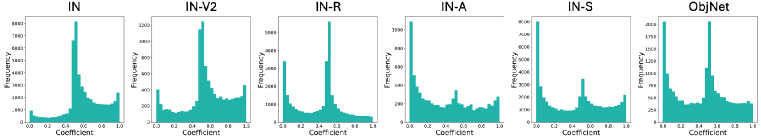
Figure 1: Distribution of interpolation coefficients. Histograms of sample-wise interpolation coefficients induced by the X-entropy ratio between two models (ZS and FT). Oracle coefficient estimates vary significantly within a domain (IN) and across domains (IN v.s. IN-V2/R/A/S/ObjNet) regarding symmetry and skewness.

Setup and hypothesis. We assess the top-1 classification accuracy of several approaches on ImageNet-1K (IN) (Russakovsky et al., 2015) and distribution-shifted benchmarks IN-V2/R/A/S/ObjNet (Recht et al., 2019; Hendrycks et al., 2021a; b; Wang et al., 2019; Barbu et al., 2019) by fine-tuning the CLIP ViT-B/32  (Radford et al., 2021) on IN. Besides the individual models (zero-shot; ZS and fine-tuned; FT), we include a representative static interpolation method, WiSE-FT (Wortsman et al., 2022b), which determines the interpolation coefficient $\lambda$ via grid search on the ID validation set. Then, we implement two oracle interpolation methods: Dynamic Interpolation$\dagger$ per domain and per sample. For the domain-wise dynamic interpolation, oracle coefficients $\lambda^{*}(\mathcal{X})$ are determined by grid search over all test samples within each domain $\mathcal{X}$, such as art or sketch. In contrast, for sample-wise oracle interpolation coefficients $\lambda^{*}(x)$, we use negative X-entropy to measure models’ expertise on a specific input $x$, which results in $\lambda^{*}(x)=\exp(-l(f(x;\theta_{1}),y))/(\exp(-l(f(x;\theta_{0}),y))+\exp(-l(f(x;\theta_{1}),y)))$. Note that we can regard the model $f(x;\theta)$ as an estimator of a conditional probability density function, e.g., $p_{\theta}(y|x)$. Then, given the equality between the X-entropy over the one-hot label and negative log-likelihood, $\lambda^{*}(x)$ can be interpreted as a posterior of Bernoulli distribution in the noise-contrastive estimation (Gutmann & Hyvärinen, 2010), i.e., $\lambda^{*}(x)=p_{\theta_{1}}(y|x)/(p_{\theta_{0}}(y|x)+p_{\theta_{1}}(y|x))$, which models the probability whether a data $(x,y)$ comes from the distribution $p_{\theta_{1}}(y|x)$. See Appendix A.1 for more.

In this experiment, we hypothesize that (1) Fine-grain interpolation, which adapts coefficients at a finer level (such as the sample level), can lead to substantial improvements compared to static interpolation, such as WiSE-FT. (2) Per-sample interpolation coefficients can effectively estimated with X-entropy-based model expertise measurement.

Results and interpretations. We verify our hypothesis in Table 1. Here, the domain-wise and sample-wise dynamic interpolation methods perform far better than individual models or static interpolation. Moreover, compared with the domain-wise interpolation method, sample-wise interpolations show much higher performance in all cases. This supports our hypotheses that fine-grain interpolation leads to better downstream accuracy, and the negative X-entropy can be used as a reliable estimator of per-sample model expertise to induce the interpolation coefficients.

In Figure 1, the interpolation coefficients $\lambda^{*}(x)$, computed using the X-entropy ratio (corresponding to the last row of Table 1), vary significantly within and across domains. On the one hand, the estimated coefficients are widely distributed from zero to one on all evaluation datasets. On the other hand, the distributions of coefficients also vary depending on the domain, e.g., IN and IN-A exhibit right-skewed and left-skewed distributions, respectively. This confirms that optimal coefficient estimation varies by sample, motivating the exploration of the sample-wise dynamic interpolation method. In summary, we conclude that determining proper interpolation coefficients on a sample-wise basis dramatically elevates the achievable performance of model merging-based approaches.

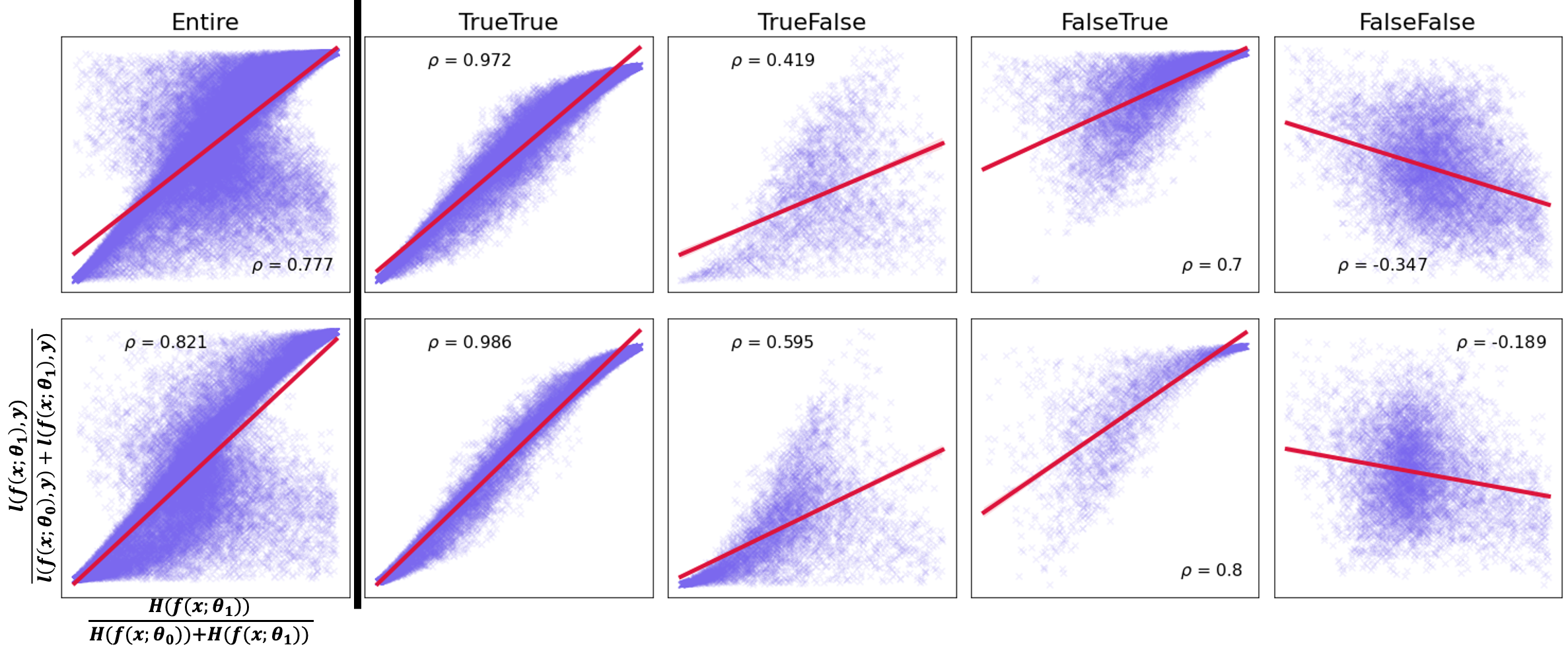
Figure 2: Correlation between entropy ratio and X-entropy ratio. We split each test set into four subsets (TrueTrue, TrueFalse, FalseTrue, FalseFalse) based on the correctness of two models’ predictions (ZS and FT). On each split and the entire data, we show scatter plots of the entropy ratio (x-axis) and x-entropy ratio (y-axis) computed by two models with corresponding Pearson correlations. The top and bottom rows denote results from ImageNet and ImageNet-R. Results imply that the entropy ratio strongly correlates with the X-entropy ratio overall, except FalseFalse case, wherein we could not expect satisfactory performance for individual models and interpolation methods as an inherent limitation given fixed individual models.

3 Method

3.1 Revisiting Entropy as a Measure of Model Expertise

While the pilot study in the previous section provides encouraging results, those oracle methods cannot work in practice. This is because we do not have access to the ground truth labels for incoming test samples. This leads us to the question: how can we reliably estimate the interpolation coefficient solely based on the test input $x$? There is extensive literature which adopts entropy as a proxy of X-entropy (Grandvalet & Bengio, 2004; Chapelle & Zien, 2005; Shu et al., 2018; Wang et al., 2021; Prabhu et al., 2021). The rationale behind using entropy as a surrogate is grounded in the observation that the entropy of a sample’s prediction distribution strongly correlates with X-entropy, even under distribution shifts (Wang et al., 2021) those models have not explicitly trained on. This work presents the first attempt to leverage the sample-wise entropy to measure each model’s expertise to determine the interpolation coefficients given each test sample. It is worth noting that this approach differs from AdaMerging (Yang et al., 2024b), which seeks to learn a global coefficient inducing a single merged model to minimize the expected entropy over the entire test set.

In this section, we will show that entropy is well-correlated with X-entropy and can thus be used to estimate model expertise. Specifically, we divide the test set into four splits, $\{$TrueTrue, TrueFalse, FalseTrue, FalseFalse$\}$, based on the correctness of predictions made by two models (zero-shot and fine-tuned CLIP). For example, TrueTrue represents the set $\{(x_{i},y_{i})|f(x_{i};\theta_{0})=y_{i}\;\text{and}\;f(x_{i};\theta_{1})=y_{i}\}$. We then compute the Pearson correlation coefficients between entropy and X-entropy within each split. Figure 2 shows scatter plots with fitted regression lines of the entropy and X-entropy ratios between two models on IN (top) and IN-R (bottom). Specifically, we plot $\frac{H(f(x;\theta_{0}))}{H(f(x;\theta_{0}))+H(f(x;\theta_{1}))}$ and $\frac{l(f(x;\theta_{0}),y)}{l(f(x;\theta_{0}),y)+l(f(x;\theta_{1}),y)}$ for entire test samples and compute Pearson correlation coefficient between them, where $H$ denotes the entropy.

Here, aside from the FalseFalse case where both models failed to produce reliable predictions, we observe strong correlations (Schober et al., 2018) across the remaining splits and the entire dataset. This implies that entropy is a reasonable proxy to the X-entropy for estimating per-sample model expertise and, ultimately, computing sample-wise interpolation coefficients.

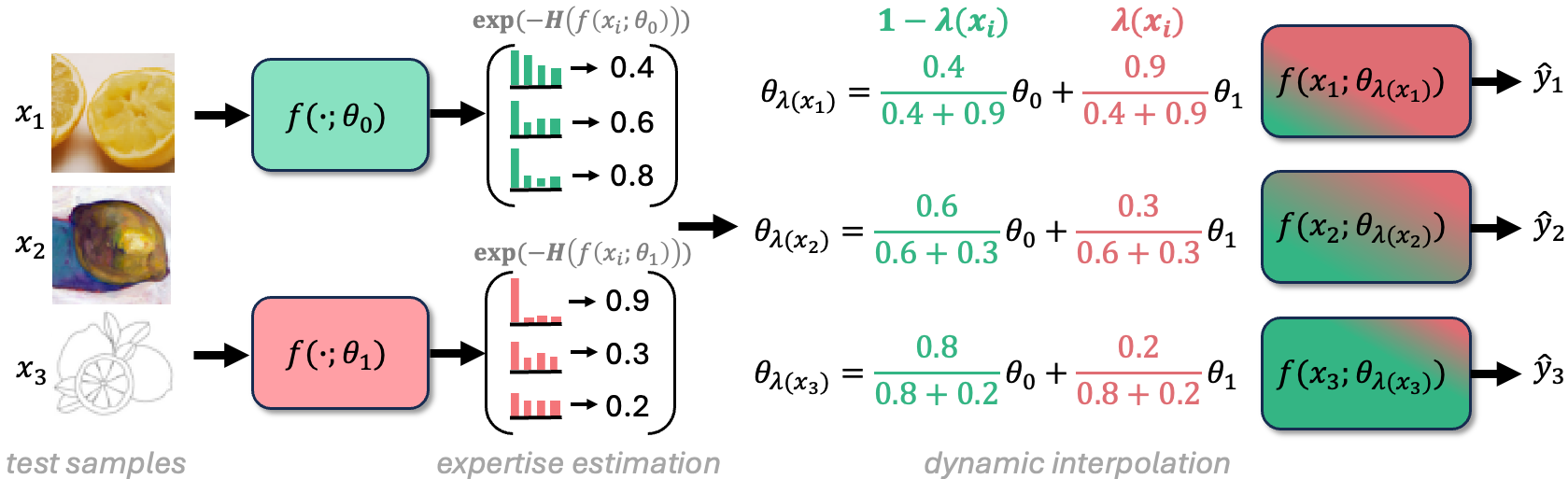
Figure 3: Framework overview. DaWin estimates per sample model expertise (exponentiated negative entropy) and then produces coefficients based on the relative expertise of models for dynamic interpolation.

3.2 Dynamic Interpolation via Entropy Ratio

After confirming a strong correlation between the entropy and X-entropy, we propose a new dynamic weight interpolation, DaWin, by defining sample-wise interpolation coefficients $\lambda(x)$ as below:

$$\lambda(x)=\frac{\exp(-H(f(x;\theta_{1})))}{\exp(-H(f(x;\theta_{0})))+\exp(-H(f(x;\theta_{1})))}.$$ (1)

Here, $H$ represents the entropy over the output probability distribution of model $f(\cdot;\theta)$ given input $x$. The value of $\lambda(x)$ approaches 1 when model $f(\cdot;\theta_{1})$ exhibits lower entropy (greater expertise), whereas it approaches 0 if the entropy of model $f(\cdot;\theta_{1})$ becomes higher. Figure 3 illustrates the overall framework. Intuitively, this approach is analogous to classifier selection methods (Giacinto & Roli, 2001; Ko et al., 2008), which aims to dynamically select suitable classifier(s) given a test sample. However, DaWin differs in terms of its motivation, expertise metric, and goal as we pursue finding the interpolation coefficients that may induce better performance compared with the best model selection method (See Table 5). We further discuss the connection between DaWin and the selection-based method in Sec. 6. Note that our sample-wise expertise estimations do not require any hyperparameters for computing interpolation coefficients. This eliminates the need for intensive hyperparameter tuning often required in prior works (Wortsman et al., 2022b; Ilharco et al., 2023) to achieve the best result. Meanwhile, if we assume access to all test samples simultaneously, we can refine the coefficient computation by introducing per-domain expertise offset terms (please see Appendix A.1). We use this offset adjustment by default, which brings consistent improvements.

Sample-wise entropy valley hypothesis. One of the most popular hypotheses that explain the success of weight interpolations is linear mode connectivity (LMC; Frankle et al. (2020)), which ensures that interpolated models are also laid on good solution space as well as low-loss converged individual models. Although entropy is a concave function that denies the LMC in nature, we believe that a similar statement can be claimed, which we refer to sample-wise entropy valley as follows:

1. There exists $\lambda$ such that $\mathbb{E}_{x}[H(f(x;\lambda\theta_{0}+(1-\lambda)\theta_{1})]\leq\min\{\mathbb{E}_{x}[H(f(x;\theta_{0}))],\mathbb{E}_{x}[H(f(x;\theta_{1}))]\}$.

2. Given $\lambda$ obeyed to (i) and evidence of sample-wise linear feature connectivity (Zhou et al., 2023), there also exists $\lambda(x)$ such that $\mathbb{E}_{x}[H(f(x;\lambda(x)\theta_{0}+(1-\lambda(x))\theta_{1})]\leq\mathbb{E}_{x}[H(f(x;\lambda\theta_{0}+(1-\lambda)\theta_{1})]$.

As empirical validation of this hypothesis, Figure 6 shows that the interpolated model actually induces smaller entropy than individuals (i) on average, and DaWin achieves lower entropy than static interpolation (ii). Given the strong correlation between entropy and X-entropy, this hypothesis advocates the benefit of DaWin than static interpolation methods.

3.3 Efficient Dynamic Interpolation by Mixture Modeling

Although our primary goal is to achieve better downstream task performance by way of dynamic interpolation, performing interpolation on every sample inevitably increases the inference-time computation, with the cost scaling linearly with the number of model parameters (Lu et al., 2024). To ensure practicality while pursuing state-of-the-art downstream task performance, we devise an efficient dynamic interpolation method by leveraging mixture modeling.

Let $\{x_{i}\}_{i=1}^{N}$ denote the $N$ test samples and $\{\lambda(x_{i})\}_{i=1}^{N}$ the corresponding interpolation coefficients computed by DaWin framework. Note that $\lambda(x_{i})\in[0,1]$ for all $i=1,\dots,N$, and they can be regarded as sampled observations from some Beta distributions. Then, we accurately model the probability density function of interpolation coefficients via Beta mixture model as follows:

$$\Lambda_{i}\sim\Sigma_{k=1}^{K}\pi_{k}\text{Beta}(\lambda(x_{i});a_{k},b_{k}),$$

where $\Lambda_{i}$ indicates random variables of $\lambda(x_{i})$ and $\{\pi_{k}\}_{k=1}^{K}$ are the prior probabilities for each Beta distribution $\text{Beta}(\cdot;a_{1},b_{1}),...,\text{Beta}(\cdot;a_{K},b_{K})$. We initialize the parameters $(a_{k},b_{k})_{k=1}^{K}$ randomly for each Beta distribution and estimate the initial membership of each sample via $K$-means clustering. Then, the expectation-maximization (EM) algorithm is adopted to iteratively refine the parameters of the Beta mixture and the membership inference quality. This process only takes around 30 seconds for 50K samples. Finally, given a test sample $x_{i}$, we infer the membership of that sample via maximum likelihood $k^{*}=\operatorname*{arg\,max}_{k}\text{Beta}(\lambda(x_{i});a_{k},b_{k})$, and use the mean of the corresponding Beta distribution $\frac{a_{k^{*}}}{a_{k^{*}}+b_{k^{*}}}$. This approach significantly reduces the computational burden of sample-wise dynamic interpolation from $N$ (number of test samples) to $K$ (number of pre-defined clusters), where $K\ll N$. We outline the detailed procedures of DaWin in Algorithm 1 (Appendix A.1).

4 Experiments

4.1 Setup

Tasks and datasets. We validate DaWin on two scenarios: (1) robust fine-tuning (Wortsman et al., 2022b) and (2) multi-task learning (Ilharco et al., 2022) with focusing on the top-1 classification accuracy (Acc). Following robust fine-tuning literature (Wortsman et al., 2022b; Kumar et al., 2022), we use ImageNet-1K and its five OOD variants, ImageNet-V2, ImageNet-R, ImageNet-A, ImageNet-Sketch, and ObjectNet, to evaluate robustness under distribution shifts. For multi-task learning, we follow the standard evaluation protocol (Ilharco et al., 2022; Yang et al., 2024b) using eight benchmark datasets: SUN397, Cars, RESISC45, EuroSAT, SVHN, GTSRB, MNIST, and DTD. Please see the Appendix A.2 for the omitted references and description for each dataset.

Models and baselines. For robust fine-tuning, we adopt CLIP ViT-{B/32, B/16, L/14} (Radford et al., 2021) as zero-shot (ZS) models to ensure a fair comparison with (Wortsman et al., 2022b; a; Ilharco et al., 2022; Yang et al., 2024b), and fine-tuned (FT) checkpoints for each backbone from Jang et al. (2024) (see details in Appendix A.2). For the weight interpolation baseline methods, we include WiSE-FT (Wortsman et al., 2022b), Model Soup (Wortsman et al., 2022a), and Model Stock (Jang et al., 2024), along with the traditional output ensemble method. In addition, we consider several state-of-the-art robust fine-tuning methods such as LP-FT (Kumar et al., 2022), CAR-FT (Mao et al., 2024), FLYP (Goyal et al., 2023), Lipsum-FT (Nam et al., 2024), and CaRot (Oh et al., 2024). For multi-task learning, we use CLIP ViT-B/32 as our backbone and consider the model merging baselines as follows: weight averaging, Fisher Merging (Matena & Raffel, 2022), RegMean (Jin et al., 2023), Task Arithmetic (Ilharco et al., 2023), Ties-Merging (Yadav et al., 2023), AdaMerging (Yang et al., 2024b), and Pareto Merging (Chen & Kwok, 2024). For a fair comparison, we do not experiment with other training-intensive dynamic methods that introduce lots of additional parameters (Tang et al., 2024), the post-hoc methods (Yang et al., 2024a) and test-time prompt tuning (Shu et al., 2022), which are orthogonal to baseline and our methods. For DaWin, we set $K$ to 3, 5, 2 for ViT-{B/32, B/16, L/14} in the robust fine-tuning and $K=1$ in the multi-task setups.

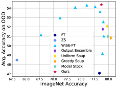
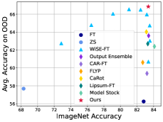
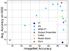
Figure 4: ID and OOD trade-off analysis. Trade-offs in terms of ID and OOD classification accuracy on ImageNet distribution shift benchmarks with CLIP ViT-{B/32, B/16, L/14} from left to right. The hyperparameter grid of WiSE-FT is set to $\{0.1,0.2,...,0.9\}$. DaWin achieves performance beyond the Pareto-optimal points given two models, ZS and FT (See Figure A in Appendix A.3 for more results).

4.2 Results on Robust Fine-tuning

Better performance trade-off between ID and OOD. In Figure 4, we present the accuracy for ID ($x$-axis) and OOD average ($y$-axis) across three backbone models, along with baseline performance. Achieving superior ID/OOD trade-offs beyond or even comparable to the WiSE-FT hyperparameter sweep is challenging. Nevertheless, DaWin provides a remarkably better performance trade-off compared to baseline methods. It is also worth noting that DaWin does not require any hyperparameter tuning. Instead, it dynamically generates interpolation coefficients solely based on the trained models’ output. This distinguishes DaWin from other hyperparameter-intensive fine-tuning such as CaRot (Oh et al., 2024) and Lipsum-FT (Nam et al., 2024) or existing interpolation methods (Wortsman et al., 2022b). Table 2 provides detailed train/inference costs and ID/OOD accuracies. Compared with Model Soups (Uniform and Greedy Soups) and Model Stock, which require more than two models to ensure diversity among interpolation candidate models (Wortsman et al., 2022a) or periodic interpolations during training (Jang et al., 2024), DaWin operates with only a single fine-tuned model while achieving significantly better performance trade-off. These trends hold across other backbones (see Tables 4.2 and 4.2), verifying DaWin’s generality in terms of modeling scale. Although DaWin compromises the inference-time efficiency for accuracy, given that existing works typically require hyperparameter tuning in practice (Wortsman et al., 2022b), relative computation overhead is minor given that we set $(K+M)\lesssim H$ in all our experiments (See Figure 8).

Table 2: Accuracy on ImageNet (ID) and its OOD for CLIP ViT-B/32. Cost (T, I) denote the number of training runs required to build the final model and the number of evaluations during inference, respectively. Given $M$ models, $N$ denotes the number of test samples, and $H$ and $K$ denote the size of the hyperparameter grid and the number of mixture components, respectively. Note that $(K+M)\lesssim H$ in all our experiments. Coefficients for Output ensemble and WiSE-FT were picked by grid search on ID validations set.

Method	Cost (T)	Cost (I)	ImageNet Acc (ID)	Avg. Acc on OOD
ZS	-	$\mathcal{O}(1)$	63.35	48.48
FT	1	$\mathcal{O}(1)$	78.35	47.08
Output ensemble	1	$\mathcal{O}(M)$	78.97	51.76
WiSE-FT (Wortsman et al., 2022b)	1	$\mathcal{O}(H)$	79.14	51.02
Uniform Soup (Wortsman et al., 2022a)	48	$\mathcal{O}(1)$	79.76	52.08
Greedy Soup (Wortsman et al., 2022a)	48	$\mathcal{O}(1)$	80.42	50.83
Model Stock (Jang et al., 2024)	2+$\alpha$	$\mathcal{O}(1)$	79.89	50.99
DaWin w/o mixture modeling	1	$\mathcal{O}(N+M)$	78.71	54.41
DaWin	1	$\mathcal{O}(K+M)$	78.70	54.36

Ablation study. We explore alternative metrics beyond entropy for estimating sample-wise model expertise, as shown in Figure 5. Specifically, we consider four different pseudo label (PL) approaches (Lee et al., 2013) to replace the entropy, $\{\hat{y},\tilde{y}\}\times\{\text{soft},\text{hard}\}$, where $\hat{y}=\frac{1}{2}f(x;\theta_{0})+\frac{1}{2}f(x;\theta_{1})$ and $\tilde{y}=f(x;\frac{1}{2}\theta_{0}+\frac{1}{2}\theta_{1})$. The settings $\{\text{soft},\text{hard}\}$ indicate whether the argmax operation is applied to PL or not. We observe that some PLs slightly outperform entropy in terms of ID accuracy but bring no gains in OOD accuracy. To maintain simplicity in line with Occam’s razor (Good, 1977), we adopt entropy as the expertise metric on unlabeled test samples.

Figure 5: Effectiveness of our expertise metric. We evaluate five different expertise metrics on ID (left) and OOD (right). Entropy ($H$) behaves like loss ($l$) with the pseudo labels, where its performance nearly matches or surpasses the best-performing $l$ though its simplicity.

Table 3: Accuracy on ImageNet (ID) and distribution shifts (OOD) for CLIP ViT-B/16.

Method	ID	OOD Avg.
ZS	68.3	57.7
FT	82.8	56.3
LP-FT (Kumar et al., 2022)	82.5	61.3
CAR-FT (Mao et al., 2024)	83.2	59.4
FLYP (Goyal et al., 2023)	82.7	60.6
Lipsum-FT (Nam et al., 2024)	83.3	62.7
CaRot (Oh et al., 2024)	83.1	64.0
Output ensemble	83.4	63.6
WiSE-FT (Wortsman et al., 2022b)	83.5	64.2
Model Stock (Jang et al., 2024)	84.1	62.4
DaWin	83.4	66.9

Table 4: Accuracy on ImageNet (ID) and distribution shifts (OOD) for CLIP ViT-L/14.

Method	ID	OOD Avg.
ZS	75.5	70.9
FT	87.0	70.6
FLYP	86.2	71.4
CaRot	87.0	74.1
Output ensemble	87.3	73.3
WiSE-FT	87.3	73.2
Model Stock	87.7	73.5
DaWin	86.9	76.0

Entropy analysis. Our DaWin method is built on the correlation between entropy and X-entropy. While the analyses from Sec. 2.2 support using entropy as a proxy of X-entropy, it does not answer how the entropy of interpolated final models behaves. To explore this, we analyze the average entropy of interpolated models generated by DaWin in Figure 6. We see that the simple weight averaging (WA) produces lower entropy compared to individual models, and our DaWin achieves the lower entropy in all cases. This indicates that DaWin’s expertise-based interpolation successfully weighs individual experts for accurate prediction and decreases per-sample entropy accordingly. In Sec. 6, we further provide a discussion on the analytic behavior of DaWin’s weighting strategy.

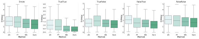
Figure 6: Entropy comparison on ImageNet-A for CLIP ViT-B/32. We visualize the average entropy from each method on the entire dataset and four different splits based on the correctness of zero-shot (ZS) and fine-tuned (FT) models. Compared with individual models, weight averaging (WA) induces lower entropy overall, and our DaWin achieves the lowest entropy across all splits (See Figure F in Appendix for full results).

Applications: dynamic selection and dynamic output ensemble. Given that DaWin is motivated by the concept of “entropy as a measure of model expertise,” we can extend this beyond weight interpolation to two other approaches, dynamic classifier selection (DCS; Giacinto & Roli (2001); Britto et al. (2014)) and dynamic output ensemble (DOE; Alam et al. (2020); Li et al. (2023)).

Table 5: Results of per-sample dynamic classifier selection (DCS), dynamic output ensemble (DOE), and dynamic weight interpolation (DaWin) on ImageNet (ID) and under distribution shifts (OOD) for different CLIP ViT backbone models.

	Model	Method
		FT	DCS	DOE	DaWin
ID	B/32	78.35	78.59	78.71	78.71
	B/16	82.80	82.15	83.24	83.38
	L/14	87.07	86.53	87.07	86.88
OOD	B/32	47.08	52.87	52.71	54.41
	B/16	56.25	64.90	64.85	66.85
	L/14	70.59	74.71	75.14	76.01

To be specific, DCS aims to select the most suitable classifier for each test sample based on the competence (referred to as expertise in our terminology) among multiple classifiers. We provide the results of DCS by adopting entropy as a competence measurement for classifier selection, i.e., selecting a lower entropy model per sample. Besides, we also present a dynamic output ensemble (DOE) by our $\lambda(x)$ directly on the output probability space rather than weight space. In Table 5, we see that entropy-based DCS and DOE bring large performance gains compared with a single fine-tuned model (FT), while the DaWin achieves the largest gain. This implies that users can flexibly build their dynamic system using test sample entropy according to their budget and performance criteria.

4.3 Results on Multi-task Learning

We now evaluate existing merging approaches and our DaWin on multi-task learning benchmarks with CLIP ViT-B/32. Following the standard evaluation protocol (Yang et al., 2024b), we have $M$ tasks and models individually fine-tuned on each task (where $M=8$). We do not know where each test sample arises from during evaluation and cannot choose true experts per domain. While both AdaMerging and DaWin use unlabeled testset, DaWin produces dynamic merged models given tasks or samples, whereas AdaMerging induces a single merged model for all tasks by default.

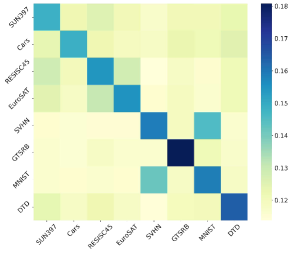
Figure 7: Merging coefficient visualization. We visualize DaWin’s coefficients across 8 datasets (columns) with 8 fine-tuned models (rows).

Here, we modify the interpolation formula in Sec. 2.1 into task arithmetic formulation, i.e., given weights of pre-trained model $\theta_{0}$ and fine-tuned models $\{\theta_{j}\}_{j=1}^{M}$, a dynamic interpolation is defined as $\theta_{\lambda(x)}=\theta_{0}+\lambda_{0}\sum_{j=1}^{M}\lambda_{j}(x)\tau_{j}$ where $\tau_{j}=\theta_{j}-\theta_{0}$, $\lambda_{j}(x)$, and $\lambda_{0}$ denote the task vector (Ilharco et al., 2023), weight for $j$-th task vector, and scaling term (set to $0.3$ following Ilharco et al. (2023)), respectively. In Table 6, DaWin greatly outperforms advanced weight averaging methods (Jin et al., 2023) and adaptive merging methods (Chen & Kwok, 2024) that require tough training, whereby approaching a ground truth expert selection method, e.g., Individuals$\dagger$. This verifies the versatility of DaWin, which is beneficial for adapting the model on multiple tasks as well as a single-task setup. Figure 7 shows the average of estimated sample-wise coefficients (y-axis) per dataset (x-axis). DaWin assigns the highest weights to true experts (diagonal) per task and leverages relevant experts by reflecting task-wise similarity, e.g., SVHN $\Leftrightarrow$ MNIST for digit recognition and EuroSAT $\Leftrightarrow$ RESISC45 for scenery classification.

Table 6: Multi-task learning performance. We use CLIP ViT-B/32 for evaluation across eight benchmark tasks. $\dagger$ denotes optimal-like performance using the ground truth domain indicator to select models for each domain. We report the layer-wise method for AdaMerging (Yang et al., 2024b) here, which surpasses those of the task-wise method. Note that AdaMerging and Pareto Merging both require a non-trivial amount of training.

Method	SUN397	Cars	RESISC45	EuroSAT	SVHN	GTSRB	MNIST	DTD	Avg.
Pre-trained	63.2	59.6	60.2	45.2	31.6	32.6	48.3	44.4	48.1
Jointly fine-tuned	73.9	74.4	93.9	98.2	95.8	98.9	99.5	77.9	88.9
Individuals$\dagger$	75.3	77.7	96.1	99.8	97.5	98.7	99.7	79.4	90.5
Weight Average (Ilharco et al., 2022)	65.3	63.3	71.4	72.6	64.2	52.8	87.5	50.1	65.9
Fisher Merging (Matena & Raffel, 2022)	68.6	69.2	70.7	66.4	72.9	51.1	87.9	59.9	68.3
RegMean (Jin et al., 2023)	65.3	63.5	75.6	78.6	78.1	67.4	93.7	52.0	71.8
Task Arithmetic (Ilharco et al., 2023)	55.3	54.9	66.7	75.9	80.2	69.7	97.3	50.1	68.8
Ties-Merging (Yadav et al., 2023)	65.0	64.3	74.7	75.7	81.3	69.4	96.5	54.3	72.6
AdaMerging (Yang et al., 2024b)	64.2	68.0	79.2	93.0	87.0	92.0	97.5	58.8	80.0
AdaMerging++ (Yang et al., 2024b)	65.8	68.4	82.0	93.6	89.6	89.0	98.3	60.2	80.9
Pareto Merging (Chen & Kwok, 2024)	71.4	74.9	87.0	97.1	92.0	96.8	98.2	61.1	84.8
DaWin	66.2	66.7	91.3	99.2	94.7	98.1	99.5	74.6	86.3

5 Related Work

Robust fine-tuning aims to adapt a model on a target task while preserving the generalization capability learned during pre-training. A straightforward approach injects regularization into the learning objective. For example, Ju et al. (2022) proposed a regularization motivated by Hessian analysis, Tian et al. (2023a; b) devised a trainable projection method to constrain the parameter space, CAR-FT (Mao et al., 2024) devised the context-awareness regularization, and CaRot (Oh et al., 2024) introduced a regularization based on singular values. Another line of works modifies the training procedure to keep the pre-trained knowledge by decoupling the tuning of a linear head from the entire model (Kumar et al., 2022), employing a data-dependent tunable module (Lee et al., 2023), utilizing bi-level optimization (Choi et al., 2024), or mimicking the pre-training procedure (Goyal et al., 2023). In contrast, weight interpolation approaches emerged as an effective yet efficient solution that conducts simple interpolation of individual model weights (Izmailov et al., 2018; Wortsman et al., 2022a; b; Jang et al., 2024). Unlike existing works inducing a single interpolated model, we propose a dynamic interpolation method that produces per-sample models for better adaptation.

Model merging studies mainly focus on integrating multiple models trained on different tasks into a single model to create a versatile, general-purpose multi-task model. After some seminal works in the era of foundation models (Ilharco et al., 2022; 2023; Jin et al., 2023), numerous advances have been made those aim at reducing conflict between merged parameters (Yadav et al., 2023; Yu et al., 2024; Marczak et al., 2024), merging with weight disentanglement (Wang et al., 2024; Ortiz-Jimenez et al., 2024; Jin et al., 2024), optimizing interpolation coefficients on unlabeled test samples (Yang et al., 2024b; Chen & Kwok, 2024) or learning additional modules generating per-sample/domain coefficients dynamically (Cheng et al., 2024; Lu et al., 2024; Tang et al., 2024; Yang et al., 2024a). While those methods provide huge performance gains compared with static methods such as (Wortsman et al., 2022a), they all bring extra learnable modules and training. We focus on methods that do not induce extra complex training and devise a training-free dynamic merging method, DaWin, which seeks a good trade-off between efficiency and downstream performance.

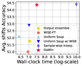
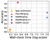
Figure 8: Accuracy and wall-clock inference time with CLIP ViT-B/32. We compare search-based methods, a test-time method (AdaMerging), and ours regarding the accuracy and inference time on robust fine-tuning (left) and multi-task learning evaluation on the SVHN dataset (right).

6 Discussion

Accuracy and runtime trade-off. While we focus on improving accuracy through model merging approaches, it is crucial to ensure the extra computation demands of DaWin during inference are manageable. Fig. 8 presents trade-offs between the accuracy and wall-clock time for various merging methods. For methods requiring hyperparameter tuning, e.g., WiSE-FT and Task Arithmetic, the wall-block time (logarithm of second) reflects a cumulative time for evaluations across all hyperparameters. For methods like DaWin or AdaMerging, we include the time required for additional workloads. In both settings, DaWin shows favorable trade-offs that outperform the most efficient one in terms of accuracy while its runtime is far less than computation-heavier methods such as per sample interpolation without mixture modeling (Sample-wise Interp.) or AdaMerging. Thus, DaWin provides a high-performing merging solution that can be flexibly adapted considering a given cost budget.

Theoretical analysis. To understand the empirical success of DaWin, we present an analytic behavior of entropy-based dynamic weight interpolation in contrast to input-independent uniform weight interpolation, which yields a uniform interpolation coefficient (Wortsman et al., 2022a).

Lemma 6.1 (Expert-biased weighting behavior of DaWin; Proof is deferred to Appendix A.4).

Suppose we have $M$ different models $\{f(\cdot;\theta_{j})\}_{j=1}^{M}$ parameterized by $\{\theta_{j}\}_{j=1}^{M}$ with a homogeneous architecture defined by $f(\cdot)$. Let $\lambda(x)=(\lambda_{1}(x),\dots,\lambda_{M}(x))$ be the sample-wise interpolation coefficient vector given $x$. If the models that render a correct prediction for $x$ always have smaller output entropy $H(\cdot)$ compared with the models rendering an incorrect prediction, DaWin’s interpolation coefficients of true experts for the sample $x$ are always greater than $\frac{1}{M}$. That is,

$$\lambda_{j\in\mathcal{J}}(x)\geq\frac{1}{M}\;\; \text{where}\;\;\mathcal{J}=\{i|\operatorname*{arg\,max}_{c}[f(x;\theta_{i})]_{c}=y\}\;\;\text{if}\;\;H(f(x;\theta_{j\in\mathcal{J}}))\leq H(f(x;\theta_{k\notin\mathcal{J}}))\;\;\forall j\;\text{and}\;k,$$

where $[f(x;\theta)]_{c}$ indicates the probability mass for class $c$. Lemma 6.1 implies that, under the entropy-dominancy assumption, DaWin always produces per-sample expert-biased coefficient vectors, which result in the interpolated models being biased towards true experts, i.e., models that produce correct prediction given $x$. This desirable behavior is aligned with the motivation of dynamic classifier selection discussed in Sec. 4.2, whereas DaWin conducts interpolation rather than selection. Meanwhile, as the number of models participating in interpolation increased, samples that at least one model correctly classifies also increased. Therefore, the coverage of DaWin for weighing the correct experts expands accordingly. This analysis endows a potential clue for remarkable gains observed in the multi-task setting, which conducts merging beyond two models (See Sec. 4.3).

Conclusion. This work has presented a novel training-free dynamic weight interpolation method, DaWin, that estimates the sample-wise model expertise with output entropy to produce reliable per-sample interpolation coefficients. We further proposed a mixture modeling approach, which greatly enhances computational efficiency. We then extensively evaluated DaWin with three different backbone models on two application scenarios, robust fine-tuning and multi-task learning, spanning 14 benchmark classification tasks. Regarding ID/OOD trade-offs in robust fine-tuning setup and overall accuracy in multi-task setup, DaWin consistently outperforms existing methods, implying its generality. This empirical success was further explained by discussing an analytic behavior of DaWin.

Acknowledgments

We thank the researchers and interns at NAVER AI Lab – Byeongho Heo, Taekyung Kim, Sanghyuk Chun, Sehyun Kwon, Yong-Hyun Park, and Jaeyoo Park – for their invaluable feedback. Most of the experiments are based on the NAVER Smart Machine Learning (NSML) platform (Sung et al., 2017). We also appreciate on the constructive comments from Max Khanov, Hyeong Kyu Choi, and Seongheon Park at University of Wisconsin–Madison. This work was supported by Institute of Information & communications Technology Planning & Evaluation (IITP) grant funded by the Korea government (MSIT) (RS-2022-00143911, AI Excellence Global Innovative Leader Education Program) and the National Research Foundation of Korea (NRF) grant funded by the Korea government(MSIT)(RS-2024-00457216, 2022R1A4A3033874)

Appendix A Appendix

We provide the following items in this Appendix:

• (A.1) Algorithm and additional details on DaWin

• (A.2) Additional details on the experiment setup

• (A.3) Additional empirical results

• (A.4) Missing proof

• (A.5) Limitation and future work

A.1 Algorithm and additional details on DaWin

Input: Test samples $X=\{x_{i}\}_{i=1}^{N}\in\mathbb{R}^{N\times D}$, models $f(\cdot;\theta_{0})$ and $f(\cdot;\theta_{1})$ of the same architecture, entropy function $H(\cdot)$, and the number of mixture component $K$

for $i=1,\dots,N$ do

       ($H_{i,0},H_{i,1})\leftarrow(H(f(x_{i};\theta_{0})),H(f(x_{i};\theta_{1})))$

        // Per-sample model expertise

       if offset adjustment then

             $\lambda(x_{i})\leftarrow\frac{\exp(-H_{i,1})+O(X)/T(X)}{\exp(-H_{i,0})+\exp(-H_{i,1})+O(X)}$

      else

             $\lambda(x_{i})\leftarrow\frac{\exp(-H_{i,1})}{\exp(-H_{i,0})+\exp(-H_{i,1})}$

              // Per-sample interp. coefficient

            

       end if

      

end for

bmm $\leftarrow$ BetaMixture($\{\lambda(x_{i})\}_{i=1}^{N}$;$K$).fit()

$\{m_{i}\}_{i=1}^{N}\leftarrow$ bmm.predict($X$)

  // Membership inference on test samples

for $k=0,\dots,K-1$ do

       $X_{k}\leftarrow X[\mathbb{I}(m_{i}==k),:]$

       $\lambda(X_{k})\leftarrow$ bmm[$k$].mean()

       $\theta_{\lambda(X_{k})}\leftarrow(1-\lambda(X_{k}))\theta_{0}+\lambda(X_{k})\theta_{1}$

        // Cluster-wise dynamic interp.

      

end for

Algorithm 1 Procedure for training-free dynamic weight interpolation (DaWin)

Incorporating domain-wise expertise.

While the eq equation 1 yields sample-wise interpolation coefficients solely based on the per-sample expertise estimation, if we can access the whole test samples simultaneously, we can refine the coefficient computation by introducing domain-wise offset terms. These terms are automatically estimated by the per-domain entropy of each model. Given the significant performance improvements with domain-wise dynamic interpolation (c.f. Table 1), we expect domain-wise expertise per model can be a complimentary benefit to compute the interpolation coefficient. Therefore, we modify the sample-wise coefficient term in Eq. 1 as below:

$$\lambda(x) =\frac{\exp(-H(f(x;\theta_{1})))+O({X})/T({X})}{\exp(-H(f(x;\theta_{0})))+\exp(-H(f(x;\theta_{1})))+O({X})},$$ (2)

$$O(X) =\frac{1}{2}(\frac{\text{std}(H(f(X;\theta_{0})))}{\text{mean}(H(f(X;\theta_{0})))}+\frac{\text{std}(H(f(X;\theta_{1})))}{\text{mean}(H(f(X;\theta_{1})))})\quad\;T(X)=\frac{H(f(X;\theta_{0}))+H(f(X;\theta_{1}))}{H(f(X;\theta_{0}))},$$

where $O({X})$ and $T({X})$ denote the per-domain offset (formulated as an average coefficient of variation) and relative domain expertise terms, respectively. By incorporating domain-wise expertise, DaWIN offers more stable dynamic interpolation coefficients, correcting some of the inaccuracies in sample-wise estimation (see Table A). It is worth noting that these sample-wise and domain-wise expertise estimations do not require any hyperparameters for computing interpolation coefficients. This eliminates the need for intensive hyperparameter tuning that is often required in prior works (Wortsman et al., 2022b; Ilharco et al., 2023) to achieve the best performance.

X-entropy ratio and likelihood ratio.

Let $f(x;\theta)=p_{\theta}(y|x)$ be a classifier parameterized with $\theta$ that models the ground truth conditional probability distribution $p(y|x)$. Given that we observe one-hot encoded target labels so that $l(f(x;\theta),y)=-\log(p_{\theta}(y|x))$, then we can rewrite the oracle sample-wise coefficient in Sec 2.2 as follow, $\lambda^{*}(x)=p_{\theta_{1}}(y|x)/(p_{\theta_{0}}(y|x)+p_{\theta_{1}}(y|x))$.

Details on Beta Mixture Model (BMM) with Expectation Maximization algorithm.

To enhance the inference-time efficiency of dynamic interpolation, we propose a mixture modeling approach over the estimated per-sample interpolation coefficients to reduce the number of interpolation operations from $N$ (entire test sample) to $K$ (pre-defined number of mixture components). Here, we elaborate on the detailed procedure of Beta Mixture Modeling.

We have coefficient estimates over $N$ test samples via Eq. 1 or Eq. 2 as $\{\lambda(x_{i})\}_{i=1}^{N}$. Our goal is to model those coefficients with a mixture of $K$ Beta distributions as below:

$$\text{Beta}(\lambda(x_{i});a_{k},b_{k})=\frac{\Gamma(a_{k}+b_{k})}{\Gamma(a_{k})\Gamma(b_{k})}\lambda(x_{i})^{a_{k}-1}(1-\lambda(x_{i}))^{b_{k}-1}$$ (3)

$$p(\lambda(x_{i}))=\sum_{k=1}^{K}\pi_{k}\text{Beta}(\lambda(x_{i});a_{k},b_{k})$$ (4)

where $a_{k}>0$ and $b_{k}>0$ are the shape parameters of component $k$, $\Gamma(\cdot)$ and $\pi_{k}$ denote the Gamma function and mixing prior probabilities for each Beta component satisfying $\sum_{k=1}^{K}\pi_{k}=1$ and $\pi_{k}\geq 0$. We first initialize the responsibilities $\{\gamma_{ik}\}$ by applying K-Means clustering to $\{\lambda(x_{i})\}$ to assign the initial membership per each observation to one of $K$ components. We also initialize the parameter estimates of BMM as below:

$$\text{Mixing Priors}(\pi_{k}):\pi_{k}^{(0)} =\frac{N_{k}^{(0)}}{N},\quad\text{where}\;\;N_{k}^{(0)}=\sum_{i=1}^{N}\gamma_{ik}^{(0)}.$$ (5)

$$\text{Shape Parameters}(a_{k},b_{k}):a_{k}^{(0)} =C_{k}^{(0)}\times\bar{\lambda}_{k}^{0}+\epsilon,$$ (6)

$$b_{k}^{(0)} =C_{k}^{(0)}\times(1-\bar{\lambda}_{k}^{(0)})+\epsilon$$ (7)

$$\text{where}\;\;\bar{\lambda}_{k}^{(0)} =\frac{1}{N_{k}^{0}}\sum_{i=1}^{N}\gamma_{ik}^{(0)}\lambda(x_{i}),$$ (8)

$$s^{2,(0)}_{k} =\frac{1}{N_{k}^{0}}\sum_{i=1}^{N}\gamma_{ik}^{(0)}(\lambda(x_{i})-\bar{\lambda}^{(0)}_{k})^{2},$$ (9)

$$C_{k}^{(0)} =\frac{\bar{\lambda}_{k}^{0}(1-\bar{\lambda}_{k}^{0})}{s^{2,(0)}_{k}}-1,$$ (10)

where $\epsilon$ is a small positive constant to ensure numerical stability. Here, the initial shape parameters are estimated by method-of-moments (Pearson, 1936). Then, we conduct the expectation step (E-step) and the maximization step (M-step) alternatively until convergence to refine the parameter estimate as follows:

• E-step:

  • Compute log responsibilities $\text{ln}\gamma^{(t)}_{ik}$.

  • Update responsibilities $\gamma^{(t)}_{ik}=\text{exp}(\text{ln}\gamma^{(t)}_{ik})$.

• M-step:

  • Update mixing priors $\pi_{k}^{(t+1)}$.

  • Update shape parameters $a_{k}^{(t+1)},b_{k}^{(t+1)}$ using method-of-moments estimation.

• Convergence Check:

  • Compute log-likelihood $\mathcal{L}^{(t+1)},\;\;\text{where}\;\mathcal{L}^{(t)}=\sum_{i=1}^{N}\text{ln}p(\lambda({x_{i}}))$

  • If $|\mathcal{L}^{(t+1)}-\mathcal{L}^{(t)}|<\text{tolerence}$, stop the iterations.

Then, we get the estimated parameter $\Theta=\{\pi_{k},a_{k},b_{k}\}_{k=1}^{K}$ of BMM to infer per-sample weight interpolation coefficients.

A.2 Additional details on the experiment setup

In this section, we provide extended details for task definition, baseline methods, and implementation details. Some contents might be duplicated from the main paper.

A.2.1 Tasks and Datasets

We validate DaWin on two scenarios: (1) robust fine-tuning (Wortsman et al., 2022b) and (2) multi-task learning (Ilharco et al., 2022) with focusing on the top-1 classification accuracy (Acc). Following robust fine-tuning literature (Wortsman et al., 2022b; Kumar et al., 2022), we use ImageNet-1K (Russakovsky et al., 2015) and its five variants, ImageNet-V2 (Recht et al., 2019), a post-decade reproduced version of the original ImageNet test set by following the dataset generating process of ImageNet, ImageNet-R (Hendrycks et al., 2021a), a rendition-specific collection of 200 ImageNet classes, ImageNet-A (Hendrycks et al., 2021b), an actual examples from ImageNet test set misclassified by a ResNet-50 model over 200 ImageNet classes, ImageNet-Sketch (Wang et al., 2019), a sketch-specific collection of 1000 ImageNet classes, and ObjectNet (Barbu et al., 2019) for evaluating robustness under distribution shifts. For multi-task learning, we follow the standard evaluation protocol (Ilharco et al., 2022; Yang et al., 2024b) using eight benchmark datasets from the optical character images, traffic signs, scenery or satellite imagery, and fine-grain categorization over cars and texture: SUN397 (Xiao et al., 2016), Cars (Krause et al., 2013), RESISC45 (Cheng et al., 2017), EuroSAT (Helber et al., 2019), SVHN (Yuval, 2011), GTSRB (Stallkamp et al., 2011), MNIST (LeCun, 1998), and DTD (Cimpoi et al., 2014).

A.2.2 Models and Baselines

For robust fine-tuning, we adopt CLIP ViT-{B/32, B/16, L/14} (Radford et al., 2021) as zero-shot (ZS) models to ensure a fair comparison with (Wortsman et al., 2022b; a; Ilharco et al., 2022; Yang et al., 2024b), and fine-tuned (FT) checkpoints for each CLIP ViT backbone from Jang et al. (2024). For the weight interpolation baseline methods, we include WiSE-FT (Wortsman et al., 2022b), which conducts a weight interpolation between a pre-trained model and a fine-tuned model given a single pre-defined interpolation coefficient, Model Soup (Wortsman et al., 2022a), which conducts averaging of all models’ weights (Uniform Soup) or greedily selected models’ weights (Greedy Soup) trained with different training hyperparameter configurations, and Model Stock (Jang et al., 2024), iteratively interpolate a pre-trained model with few fine-tuning model based on the cosine distance between pre-trained model weight and the fine-tuning model weights, along with the traditional output ensemble method. In addition, we consider several state-of-the-art robust fine-tuning methods such as LP-FT (Kumar et al., 2022), a two-stage method to avoid pre-trained feature distortion, CAR-FT (Mao et al., 2024), a regularized fine-tuning method leveraging context-aware prompt, FLYP (Goyal et al., 2023), a contrastive learning based fine-tuning method, Lipsum-FT (Nam et al., 2024), a regularized fine-tuning method motivated by energy score gap between zero-shot and fine-tuned models, and CaRot (Oh et al., 2024), a theory-inspired singular value regularization method.

For multi-task learning, we use CLIP ViT-B/32 as our backbone and consider the model merging baselines as follows: a simple weight averaging (Ilharco et al., 2022), Fisher Merging (Matena & Raffel, 2022), a Fisher information metric-based weighted averaging method, RegMean (Jin et al., 2023), an averaging method that minimizes $L_{2}$ distance between the averaged weight and individual weights, Task Arithmetic (Ilharco et al., 2023), a method perform arithmetic across task vectors rather the original weight vector itself which are produced by the subtractions between a pre-trained model weight and individual fine-tuned model weights, Ties-Merging (Yadav et al., 2023), a post-hoc weight refinement method mitigating conflicts between task vectors, AdaMerging (Yang et al., 2024b) and Pareto Merging (Chen & Kwok, 2024) methods those driving additional optimization procedure to a global interpolation coefficient and the conditional coefficient generation models that trained to minimize entropy over entire test sample.

A.2.3 Implementation Details

For fine-tuning CLIPs on ImageNet, Wortsman et al. (2022a) and its successor (Jang et al., 2024) conducted multiple training with different training configurations such as data augmentation, learning rate, weight decay, and random initialization seeds given fixed epochs (16) and batch size (512). Here, we use the best model weight provided by the authors of Jang et al. (2024) per each backbone. For fine-tuning weights of CLIP on multi-task learning setup, we adopt the official checkpoints from Ilharco et al. (2023) on the eight datasets.

On DaWin’s evaluation, we first get the entropy of batch test samples from the interpolation candidate models (wherein temperature scaling (Guo et al., 2017) is applied in the robust fine-tuning setup with ID validation set), then we compute interpolation coefficients by building a softmax-like model expertise ratio term with exponentiated negative entropy of each model. We further perform the mixture modeling over the batch test samples and finally conduct dynamic model merging with interpolation coefficients corresponding to estimated membership from the fitted mixture model to obtain the prediction per sample. About the Beta (on robust fine-tuning setup) and Dirichlet (on multi-tasks learning setup) mixture modeling on interpolation coefficients for DaWin, we set $K$ to 3, 5, 2 for ViT-{B/32, B/16, L/14} in the robust fine-tuning and $K=1$ in the multi-task setups. Unless otherwise mentioned, we adopt the offset adjustment term (Eq. equation 2) by default, assuming that the entire test samples per task are available and fit the Beta (and Dirichlet) mixture model on the entire coefficients per task, likewise assumption of Yang et al. (2024b; a); Chen & Kwok (2024).

A.3 Additional empirical results

Table A: Ablation study on offset adjustment. We validate the effect of using the offset adjustment term on ImageNet ID and OOD accuracy.

Model	Offset Adjustment	ID	Avg. Acc on OOD
ViT-B/32	-	78.3	54.1
	✓	78.7	54.4
ViT-B/16	-	83.1	66.6
	✓	83.4	66.9
ViT-L/14	-	86.7	75.9
	✓	86.9	76.0

We ablate the offset adjustment and expertise metric to investigate the effectiveness of the design choices of each component. Firstly, as we can see in Table A, offset adjustment consistently boosts the ID and OOD accuracy across all cases, which supports the use of domain-wise relative expertise (average entropy over all test samples) to enhance sample-wise expertise estimation.

Table B: Sensitivity analysis on sample size. We report DaWin’s ImageNet and its OOD variants’ accuracy of CLIP ViT-B/32 under varying sample wise for fitting Beta Mixture Model. DaWin shows robustness against varying sample size.

Sample size	ImageNet Accuracy	Avg. Acc on OOD
32	78.55	54.30
64	78.69	54.27
128	78.71	54.27
256	78.70	54.28
512	78.70	54.25
1024	78.71	54.24
2048	78.67	54.26
$N$	78.70	54.36

To secure inference time efficiency, we adopt the Beta mixture modeling approach on the batch-wise DaWin’s coefficients. The fitness of the Beta mixture model may be improved as the sample size is increased, whereas a smaller sample size enables more granular interpolations to be applied. Therefore, we evaluate the performance of DaWin under varying sample sizes. Table B presents the ID and OOD performance of DaWin on the ImageNet distribution shift benchmark for the CLIP ViT-B/32 backbone model. DaWin shows strong robustness against varying sample sizes.

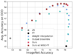
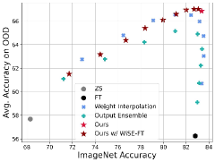
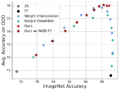
Figure A: ID and OOD trade-off analysis. We visualize performance trade-offs regarding ID and OOD classification accuracy on the ImageNet distribution shift benchmarks with CLIP ViT-$\{$B/32, B/16, L/14$\}$ from left to right. Interpolation coefficients are swept over $\{0.1,0.2,...,0.9\}$.

In Figure A, we present the results of DaWin with WiSE-FT as a plug-in augmentation on the robust fine-tuning setup. We multiply our estimated coefficients from Beta mixture by a scalar coefficient $\alpha$, e.g., $\lambda_{wise}(x)=\lambda(x)\times\alpha$. Although it brings slight benefits in the case of CLIP ViT-B/32, the WiSE-FT interpolation trace becomes almost a line on the ViT-B/16 and ViT-L/14 cases. This implies that DaWin already achieves performance beyond the Pareto-optimal trade-offs and cannot be further improved by WiSE-FT, given models $f(\cdot;\theta_{0})$ and $f(\cdot;\theta_{1})$. Meanwhile, Figure B reveals that DaWin produces larger $\lambda(x)$ for samples that are hard to recognize the target object due to overwhelming background semantics, which the pre-trained model may wrongly pay attention to.

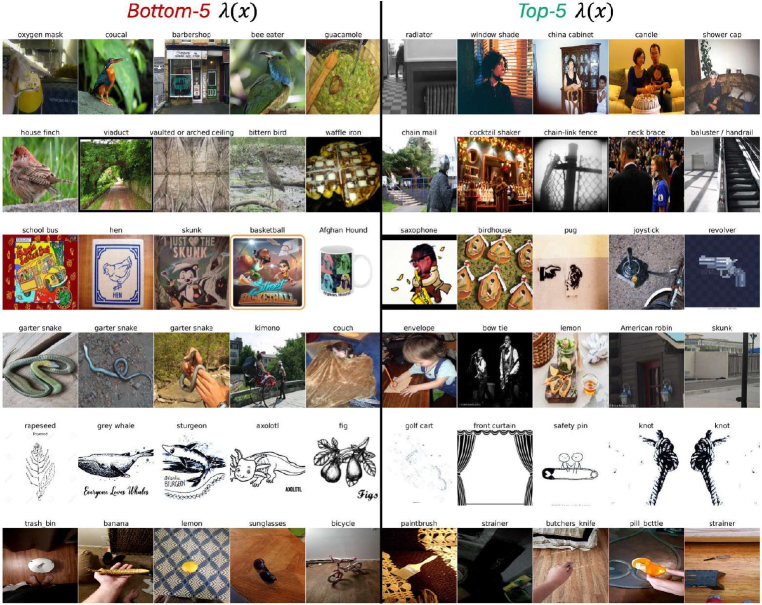
Figure B: DaWIN’s bottom-5 and top-5 estimated coefficient analysis. We visualize the images with labels corresponding to bottom-5 and top-5 sample-wise interpolation coefficients estimated by DaWIN of pre-trained and ImageNet fine-tuned CLIP ViT-B/32. Each row denotes the actual test samples from ImageNet, ImageNet-V2, ImageNet-R, ImageNet-A, ImageNet-Sketch, and ObjectNet. We see that the images corresponding to coefficients lean towards the fine-tuned model, which typically contains multiple semantics, and the object corresponding to the ground truth label is overwhelmed by other semantics.

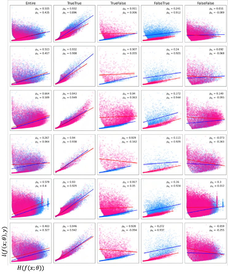
Figure C: Correlation between entropy and X-entropy. We split each testset into four subsets (TrueTrue, TrueFalse, FalseTrue, FalseFalse) based on the correctness of the two models’ predictions. On each data split and the entire dataset, we visualize scatter plots of entropy (x-axis) and cross-entropy (y-axis) computed by two models (zero-shot and fine-tuned) with corresponding Pearson correlation coefficients per model. Each row from top to bottom shows results from ImageNet, ImageNetV2, ImageNetR, ImageNetA, ImageNetSketch, and ObjectNet.

DaWin adopts entropy as a proxy of X-entropy to estimate the model expertise without access to the true target label. Figure C presents the correlation between entropy and X-entropy of the pre-trained CLIP ViT-B/32 $f(\cdot;\theta_{0})$ and ImageNet fine-tuned counterpart $f(\cdot;\theta_{1})$. Results indicate that the model producing correct predictions holds a strong correlation between entropy and X-entropy while the model failing to correctly predict test samples shows bad or no correlation. However, if at least one model success in making a correct prediction in a given sample $x$, and the entropy of the correct predictor may be smaller than that of another model, thereby DaWin would be likely to produce $\lambda(x)$ biased towards the correct predictor’s weight (See Lemma 6.1).

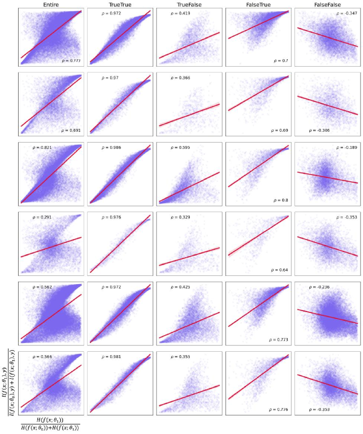
Figure D: Correlation between entropy ratio and X-Entropy ratio. We split each testset into four subsets (TrueTrue, TrueFalse, FalseTrue, FalseFalse) based on the correctness of the two models’ predictions. On each split and the entire dataset, we visualize scatter plots of entropy ratio (x-axis) and cross-entropy ratio (y-axis) computed by two models (zero-shot and fine-tuned) with corresponding Pearson correlation coefficients. Each row from top to bottom shows results from ImageNet, ImageNetV2, ImageNetR, ImageNetA, ImageNetSketch, and ObjectNet.

In Figure D, we provide the extended results of Figure 2, showing the correlations between entropy ratio and X-entropy ratio, on the whole evaluation datasets of robust fine-tuning setup. The entropy ratio approximates the X-entropy ratio overall across datasets and sub-populations of each dataset, even though for the most challenging OOD, i.e., ImageNet-A, which is constructed with natural adversarial examples, there is a weak-yet-non-trivial correlation (Schober et al., 2018) between entropy and X-entropy. Moreover, we note that weight interpolation (or output ensemble) has an advantage that elicits the correct prediction by modifying the relative feature importance (Yong et al., 2024) even though two individual models fail to produce correct predictions (i.e., in the FalseFalse case), thereby expected to outperform the model selection method (See Table 5).

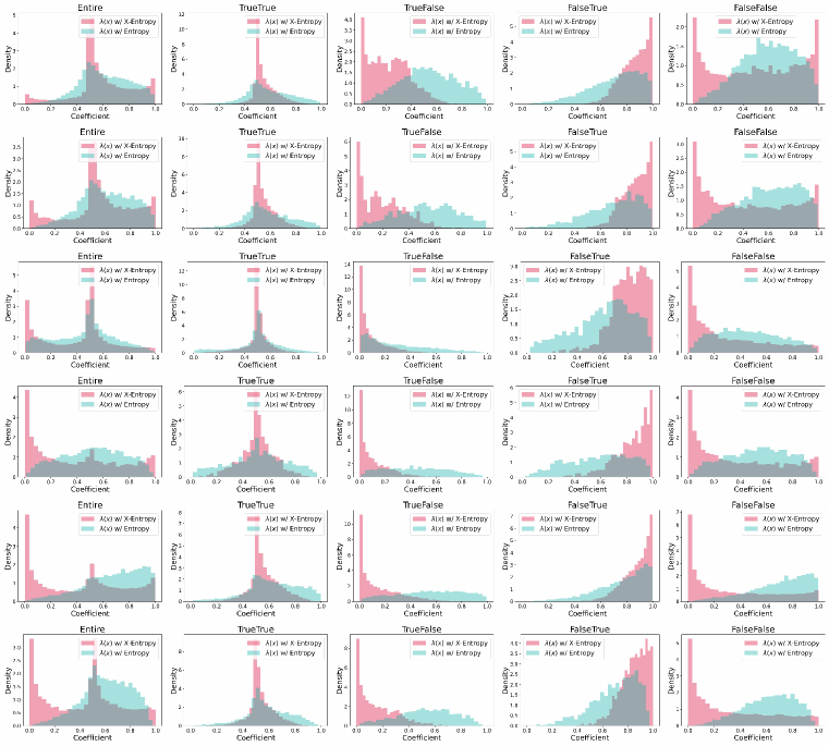
Figure E: Estimated coefficient density analysis on ImageNet distribution shift benchmarks with CLIP ViT-B/32. We visualize histograms of estimated sample-wise interpolation coefficients by the expertise ratio, which is computed using X-entropy (Oracle; we can not access it in reality) and entropy as expertise metrics. Each column denotes the splits $\{\texttt{Entire},\texttt{TrueTrue},\texttt{TrueFalse},\texttt{FalseTrue},\texttt{FalseFlase}\}$ of the test set, those are categorized by the correctness of zero-shot CLIP, and ImageNet fine-tuned CLIP’s predictions. Each low denotes the result of the test set: from ImageNet, ImageNet-V2, ImageNet-R, ImageNet-A, ImageNet-Sketch, and ObjectNet. Entropy-based coefficient estimation shows remarkably good fitness in the TrueTrue, FalseTrue splits, and produces left-skewed distribution in the case of TrueFalse, which is desired to construct the interpolated model biased towards zero-shot model weight. Overall, except the FalseFalse case, the entropy-based coefficient estimation provides reasonable alternatives to X-entropy-based oracle coefficients.

We visualize the histogram of interpolation coefficients computed by entropy and X-entropy ratio in Figure E. While the entropy-based coefficients quite diverge from the oracle X-entropy-based coefficients in some cases (e.g., TrueFalse and FalseFalse of ImageNet-Sketch and ObjectNet), the overall distributions of entropy-based coefficients show good fitness to X-entropy-based coefficients across datasets. This result supports using entropy as a proxy of X-entropy to estimate model expertise given unlabeled test-time input to determine the per-sample interpolation coefficient.

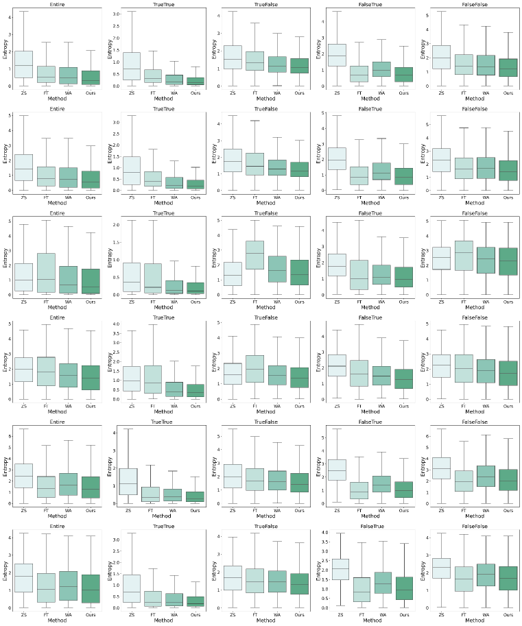
Figure F: Entropy comparison on ImageNet distribution shiftㄴ with CLIP ViT-B/32. Across IN, IN-V2, IN-R, IN-A, IN-S, and ObjNet from top to bottom, we visualize the final output entropy from each model on the entire dataset and four different splits based on the correctness of zero-shot (ZS) and fine-tuned (FT) models. Compared with individual models, weight averaging (WA) induces lower entropy overall, and our DaWin achieves the lowest entropy across all splits.

In Figure F, we provide the extended results of Figure 6, showing the average entropy over test samples, on the whole evaluation datasets of robust fine-tuning setup. In almost all of cases, weight interpolation achieves smaller entropy than individual models, and DaWin achieves the smallest entropy. This supports our sample-wise entropy valley hypothesis in Section 3.2 and helps us to understand DaWin’s great performance gains.

A.4 Missing proof

In Sec. 6, we provided an analytic behavior of DaWin, which generated true-expert biased interpolation weight vectors as below:

Lemma A.1 (Restatement of expert-biased weighting behavior of DaWin).

Suppose we have $M$ different models $\{f(\cdot;\theta_{j})\}_{j=1}^{M}$ parameterized by $\{\theta_{j}\}_{j=1}^{M}$ with a homogeneous architecture defined by $f(\cdot)$. Let $\lambda(x)=(\lambda_{1}(x),\dots,\lambda_{M}(x))$ be the sample-wise interpolation coefficient vector given $x$. If the models that render a correct prediction for $x$ always have smaller output entropy $H(\cdot)$ compared with the models rendering an incorrect prediction, DaWin’s interpolation coefficients of true experts for the sample $x$ has always greater than $\frac{1}{M}$. That is

$$\lambda_{j\in\mathcal{J}}(x)\geq\frac{1}{M}\;\quad \text{where}\;\;\mathcal{J}=\{i|\operatorname*{arg\,max}_{c}[f(x;\theta_{i})]_{c}=y\}$$

$$\text{if}\;\;H(f(x;\theta_{j\in\mathcal{J}}))\leq H(f(x;\theta_{k\notin\mathcal{J}}))\;\;\text{for all}\;\;j\;\text{and}\;k.$$

where $[f(x;\theta)]_{c}$ indicates the probability mass for class $c$.

Proof.

The proof is very straightforward, given the assumption and definitions of problem setup.

$$H(f(x;\theta_{j\in\mathcal{J}})) \leq H(f(x;\theta_{k\notin\mathcal{J}}))$$ (By assumption)

$$\exp(-H(f(x;\theta_{j\in\mathcal{J}}))) \geq\exp(-H(f(x;\theta_{k\notin\mathcal{J}})))$$

$$\lambda_{j\in\mathcal{J}}(x) \geq\lambda_{k\notin\mathcal{J}}(x) \lambda(x)$$ (By definition of )

$$\lambda_{j\in\mathcal{J}}(x) \geq\frac{1}{M} \sum_{j=1}^{M}\lambda_{j}(x)=1$$ (Given that )

∎

A.5 Limitation and future work

By following previous works (Wortsman et al., 2022b; Ilharco et al., 2023; Yang et al., 2024b), we limited our validation scope to an image classification of fully fine-tuned visual foundation models with restricted scale and architecture, e.g., CLIP ViT-$\{$B/32, B/16, L/14$\}$. Exploring DaWin on diverse model architecture (Liu et al., 2022; Gu & Dao, 2023; Liu et al., 2024), large-scale modeling setup (Dehghani et al., 2023), large language models (Yu et al., 2024; Goddard et al., 2024; Rame et al., 2023), multimodal generative models (Liu et al., 2023; Biggs et al., 2024; Nair et al., 2024), continual adaptation scenario (Marczak et al., 2024), and parameter-efficient tuning regime (Li & Liang, 2021; Hu et al., 2021; Chronopoulou et al., 2023) can be exciting future work directions.

References

- Alam et al. (2020) Kazi Md Rokibul Alam, Nazmul Siddique, and Hojjat Adeli. A dynamic ensemble learning algorithm for neural networks. Neural Computing and Applications, 32(12):8675–8690, 2020.
- Barbu et al. (2019) Andrei Barbu, David Mayo, Julian Alverio, William Luo, Christopher Wang, Dan Gutfreund, Josh Tenenbaum, and Boris Katz. Objectnet: A large-scale bias-controlled dataset for pushing the limits of object recognition models. In Advances in Neural Information Processing Systems (NeurIPS), 2019.
- Biggs et al. (2024) Benjamin Biggs, Arjun Seshadri, Yang Zou, Achin Jain, Aditya Golatkar, Yusheng Xie, Alessandro Achille, Ashwin Swaminathan, and Stefano Soatto. Diffusion soup: Model merging for text-to-image diffusion models. arXiv preprint arXiv:2406.08431, 2024.
- Bommasani et al. (2021) Rishi Bommasani, Drew A Hudson, Ehsan Adeli, Russ Altman, Simran Arora, Sydney von Arx, Michael S Bernstein, Jeannette Bohg, Antoine Bosselut, Emma Brunskill, et al. On the opportunities and risks of foundation models. arXiv preprint arXiv:2108.07258, 2021.
- Britto et al. (2014) Alceu S. Britto, Robert Sabourin, and Luiz E.S. Oliveira. Dynamic selection of classifiers—a comprehensive review. Pattern Recognition, 47(11):3665–3680, 2014. ISSN 0031-3203. doi: https://doi.org/10.1016/j.patcog.2014.05.003. URL https://www.sciencedirect.com/science/article/pii/S0031320314001885.
- Brown et al. (2020) Tom Brown, Benjamin Mann, Nick Ryder, Melanie Subbiah, Jared D Kaplan, Prafulla Dhariwal, Arvind Neelakantan, Pranav Shyam, Girish Sastry, Amanda Askell, et al. Language models are few-shot learners. Advances in neural information processing systems, 33:1877–1901, 2020.
- Chapelle & Zien (2005) Olivier Chapelle and Alexander Zien. Semi-supervised classification by low density separation. In International workshop on artificial intelligence and statistics, pp. 57–64. PMLR, 2005.
- Chen & Kwok (2024) Weiyu Chen and James Kwok. You only merge once: Learning the pareto set of preference-aware model merging. arXiv preprint arXiv:2408.12105, 2024.
- Cheng et al. (2024) Feng Cheng, Ziyang Wang, Yi-Lin Sung, Yan-Bo Lin, Mohit Bansal, and Gedas Bertasius. Dam: Dynamic adapter merging for continual video qa learning. arXiv preprint arXiv:2403.08755, 2024.
- Cheng et al. (2017) Gong Cheng, Junwei Han, and Xiaoqiang Lu. Remote sensing image scene classification: Benchmark and state of the art. Proceedings of the IEEE, 105(10):1865–1883, 2017.
- Choi et al. (2024) Caroline Choi, Yoonho Lee, Annie Chen, Allan Zhou, Aditi Raghunathan, and Chelsea Finn. Autoft: Robust fine-tuning by optimizing hyperparameters on ood data. arXiv preprint arXiv:2401.10220, 2024.
- Chronopoulou et al. (2023) Alexandra Chronopoulou, Matthew E Peters, Alexander Fraser, and Jesse Dodge. Adaptersoup: Weight averaging to improve generalization of pretrained language models. In Findings of the Association for Computational Linguistics: EACL 2023, pp. 2054–2063, 2023.
- Cimpoi et al. (2014) Mircea Cimpoi, Subhransu Maji, Iasonas Kokkinos, Sammy Mohamed, and Andrea Vedaldi. Describing textures in the wild. In CVPR, pp. 3606–3613, 2014.
- Dehghani et al. (2023) Mostafa Dehghani, Josip Djolonga, Basil Mustafa, Piotr Padlewski, Jonathan Heek, Justin Gilmer, Andreas Peter Steiner, Mathilde Caron, Robert Geirhos, Ibrahim Alabdulmohsin, et al. Scaling vision transformers to 22 billion parameters. In International Conference on Machine Learning, pp. 7480–7512. PMLR, 2023.
- Frankle et al. (2020) Jonathan Frankle, Gintare Karolina Dziugaite, Daniel Roy, and Michael Carbin. Linear mode connectivity and the lottery ticket hypothesis. In International Conference on Machine Learning, pp. 3259–3269. PMLR, 2020.
- Giacinto & Roli (2001) Giorgio Giacinto and Fabio Roli. Dynamic classifier selection based on multiple classifier behaviour. Pattern Recognition, 34(9):1879–1881, 2001. ISSN 0031-3203. doi: https://doi.org/10.1016/S0031-3203(00)00150-3. URL https://www.sciencedirect.com/science/article/pii/S0031320300001503.
- Goddard et al. (2024) Charles Goddard, Shamane Siriwardhana, Malikeh Ehghaghi, Luke Meyers, Vlad Karpukhin, Brian Benedict, Mark McQuade, and Jacob Solawetz. Arcee’s mergekit: A toolkit for merging large language models. arXiv preprint arXiv:2403.13257, 2024.
- Good (1977) IJ Good. Explicativity: a mathematical theory of explanation with statistical applications. Proceedings of the Royal Society of London. A. Mathematical and Physical Sciences, 354(1678):303–330, 1977.
- Goyal et al. (2023) Sachin Goyal, Ananya Kumar, Sankalp Garg, Zico Kolter, and Aditi Raghunathan. Finetune like you pretrain: Improved finetuning of zero-shot vision models. In Proceedings of the IEEE/CVF Conference on Computer Vision and Pattern Recognition, pp. 19338–19347, 2023.
- Grandvalet & Bengio (2004) Yves Grandvalet and Yoshua Bengio. Semi-supervised learning by entropy minimization. Advances in neural information processing systems, 17, 2004.
- Gu & Dao (2023) Albert Gu and Tri Dao. Mamba: Linear-time sequence modeling with selective state spaces. arXiv preprint arXiv:2312.00752, 2023.
- Guo et al. (2017) Chuan Guo, Geoff Pleiss, Yu Sun, and Kilian Q Weinberger. On calibration of modern neural networks. In International conference on machine learning, pp. 1321–1330. PMLR, 2017.
- Gutmann & Hyvärinen (2010) Michael Gutmann and Aapo Hyvärinen. Noise-contrastive estimation: A new estimation principle for unnormalized statistical models. In Proceedings of the thirteenth international conference on artificial intelligence and statistics, pp. 297–304. JMLR Workshop and Conference Proceedings, 2010.
- Helber et al. (2019) Patrick Helber, Benjamin Bischke, Andreas Dengel, and Damian Borth. Eurosat: A novel dataset and deep learning benchmark for land use and land cover classification. IEEE Journal of Selected Topics in Applied Earth Observations and Remote Sensing, 12(7):2217–2226, 2019.
- Hendrycks et al. (2021a) Dan Hendrycks, Steven Basart, Norman Mu, Saurav Kadavath, Frank Wang, Evan Dorundo, Rahul Desai, Tyler Zhu, Samyak Parajuli, Mike Guo, et al. The many faces of robustness: A critical analysis of out-of-distribution generalization. In IEEE Conference on Computer Vision and Pattern Recognition (CVPR), 2021a.
- Hendrycks et al. (2021b) Dan Hendrycks, Kevin Zhao, Steven Basart, Jacob Steinhardt, and Dawn Song. Natural adversarial examples. In IEEE Conference on Computer Vision and Pattern Recognition (CVPR), 2021b.
- Hu et al. (2021) Edward J Hu, Phillip Wallis, Zeyuan Allen-Zhu, Yuanzhi Li, Shean Wang, Lu Wang, Weizhu Chen, et al. Lora: Low-rank adaptation of large language models. In International Conference on Learning Representations, 2021.
- Ilharco et al. (2022) Gabriel Ilharco, Mitchell Wortsman, Samir Yitzhak Gadre, Shuran Song, Hannaneh Hajishirzi, Simon Kornblith, Ali Farhadi, and Ludwig Schmidt. Patching open-vocabulary models by interpolating weights. Advances in Neural Information Processing Systems, 35:29262–29277, 2022.
- Ilharco et al. (2023) Gabriel Ilharco, Marco Tulio Ribeiro, Mitchell Wortsman, Ludwig Schmidt, Hannaneh Hajishirzi, and Ali Farhadi. Editing models with task arithmetic. In The Eleventh International Conference on Learning Representations, 2023.
- Izmailov et al. (2018) Pavel Izmailov, Dmitrii Podoprikhin, Timur Garipov, Dmitry Vetrov, and Andrew Gordon Wilson. Averaging weights leads to wider optima and better generalization. arXiv preprint arXiv:1803.05407, 2018.
- Jang et al. (2024) Dong-Hwan Jang, Sangdoo Yun, and Dongyoon Han. Model stock: All we need is just a few fine-tuned models. European Conference on Computer Vision (ECCV), 2024.
- Jin et al. (2024) Ruochen Jin, Bojian Hou, Jiancong Xiao, Weijie Su, and Li Shen. Fine-tuning linear layers only is a simple yet effective way for task arithmetic. arXiv preprint arXiv:2407.07089, 2024.
- Jin et al. (2023) Xisen Jin, Xiang Ren, Daniel Preotiuc-Pietro, and Pengxiang Cheng. Dataless knowledge fusion by merging weights of language models. In The Eleventh International Conference on Learning Representations, 2023.
- Ju et al. (2022) Haotian Ju, Dongyue Li, and Hongyang R Zhang. Robust fine-tuning of deep neural networks with hessian-based generalization guarantees. In International Conference on Machine Learning, pp. 10431–10461. PMLR, 2022.
- Ko et al. (2008) Albert H.R. Ko, Robert Sabourin, and Alceu Souza Britto, Jr. From dynamic classifier selection to dynamic ensemble selection. Pattern Recognition, 41(5):1718–1731, 2008. ISSN 0031-3203. doi: https://doi.org/10.1016/j.patcog.2007.10.015. URL https://www.sciencedirect.com/science/article/pii/S0031320307004499.
- Krause et al. (2013) Jonathan Krause, Michael Stark, Jia Deng, and Li Fei-Fei. 3d object representations for fine-grained categorization. In ICCV workshops, pp. 554–561, 2013.
- Kumar et al. (2022) Ananya Kumar, Aditi Raghunathan, Robbie Matthew Jones, Tengyu Ma, and Percy Liang. Fine-tuning can distort pretrained features and underperform out-of-distribution. In International Conference on Learning Representations, 2022.
- LeCun (1998) Yann LeCun. The mnist database of handwritten digits. http://yann. lecun. com/exdb/mnist/, 1998.
- Lee et al. (2013) Dong-Hyun Lee et al. Pseudo-label: The simple and efficient semi-supervised learning method for deep neural networks. In Workshop on challenges in representation learning, ICML. Atlanta, 2013.
- Lee et al. (2023) Yoonho Lee, Annie S Chen, Fahim Tajwar, Ananya Kumar, Huaxiu Yao, Percy Liang, and Chelsea Finn. Surgical fine-tuning improves adaptation to distribution shifts. In The Eleventh International Conference on Learning Representations, 2023.
- Li & Liang (2021) Xiang Lisa Li and Percy Liang. Prefix-tuning: Optimizing continuous prompts for generation. In Proceedings of the 59th Annual Meeting of the Association for Computational Linguistics and the 11th International Joint Conference on Natural Language Processing (Volume 1: Long Papers), pp. 4582–4597, 2021.
- Li et al. (2023) Ziyue Li, Kan Ren, XINYANG JIANG, Yifei Shen, Haipeng Zhang, and Dongsheng Li. SIMPLE: Specialized model-sample matching for domain generalization. In The Eleventh International Conference on Learning Representations, 2023. URL https://openreview.net/forum?id=BqrPeZ_e5P.
- Liu et al. (2023) Haotian Liu, Chunyuan Li, Qingyang Wu, and Yong Jae Lee. Visual instruction tuning. Advances in neural information processing systems, 36, 2023.
- Liu et al. (2022) Zhuang Liu, Hanzi Mao, Chao-Yuan Wu, Christoph Feichtenhofer, Trevor Darrell, and Saining Xie. A convnet for the 2020s. In Proceedings of the IEEE/CVF conference on computer vision and pattern recognition, pp. 11976–11986, 2022.
- Liu et al. (2024) Ziming Liu, Yixuan Wang, Sachin Vaidya, Fabian Ruehle, James Halverson, Marin Soljačić, Thomas Y Hou, and Max Tegmark. Kan: Kolmogorov-arnold networks. arXiv preprint arXiv:2404.19756, 2024.
- Lu et al. (2024) Zhenyi Lu, Chenghao Fan, Wei Wei, Xiaoye Qu, Dangyang Chen, and Yu Cheng. Twin-merging: Dynamic integration of modular expertise in model merging. arXiv preprint arXiv:2406.15479, 2024.
- Ma & Leijon (2011) Zhanyu Ma and Arne Leijon. Bayesian estimation of beta mixture models with variational inference. IEEE Transactions on Pattern Analysis and Machine Intelligence, 33(11):2160–2173, 2011.
- Mao et al. (2024) Xiaofeng Mao, Yufeng Chen, Xiaojun Jia, Rong Zhang, Hui Xue, and Zhao Li. Context-aware robust fine-tuning. International Journal of Computer Vision, 132(5):1685–1700, 2024.
- Marczak et al. (2024) Daniel Marczak, Bartłomiej Twardowski, Tomasz Trzciński, and Sebastian Cygert. Magmax: Leveraging model merging for seamless continual learning. European Conference on Computer Vision (ECCV), 2024.
- Matena & Raffel (2022) Michael S Matena and Colin A Raffel. Merging models with fisher-weighted averaging. Advances in Neural Information Processing Systems, 35:17703–17716, 2022.
- Nair et al. (2024) Nithin Gopalakrishnan Nair, Jeya Maria Jose Valanarasu, and Vishal M Patel. Maxfusion: Plug&play multi-modal generation in text-to-image diffusion models. arXiv preprint arXiv:2404.09977, 2024.
- Nam et al. (2024) Giung Nam, Byeongho Heo, and Juho Lee. Lipsum-ft: Robust fine-tuning of zero-shot models using random text guidance. In The Twelfth International Conference on Learning Representations, 2024.
- Oh et al. (2024) Changdae Oh, Hyesu Lim, Mijoo Kim, Dongyoon Han, Sangdoo Yun, Jaegul Choo, Alexander Hauptmann, Zhi-Qi Cheng, and Kyungwoo Song. Towards calibrated robust fine-tuning of vision-language models. Advances in Neural Information Processing Systems, 2024.
- Ortiz-Jimenez et al. (2024) Guillermo Ortiz-Jimenez, Alessandro Favero, and Pascal Frossard. Task arithmetic in the tangent space: Improved editing of pre-trained models. Advances in Neural Information Processing Systems, 36, 2024.
- Pearson (1936) Karl Pearson. Method of moments and method of maximum likelihood. Biometrika, 28(1/2):34–59, 1936. ISSN 00063444, 14643510. URL http://www.jstor.org/stable/2334123.
- Prabhu et al. (2021) Viraj Prabhu, Shivam Khare, Deeksha Kartik, and Judy Hoffman. Sentry: Selective entropy optimization via committee consistency for unsupervised domain adaptation. In Proceedings of the IEEE/CVF International Conference on Computer Vision, pp. 8558–8567, 2021.
- Radford et al. (2021) Alec Radford, Jong Wook Kim, Chris Hallacy, Aditya Ramesh, Gabriel Goh, Sandhini Agarwal, Girish Sastry, Amanda Askell, Pamela Mishkin, Jack Clark, et al. Learning transferable visual models from natural language supervision. In International conference on machine learning, pp. 8748–8763. PMLR, 2021.
- Rame et al. (2023) Alexandre Rame, Guillaume Couairon, Corentin Dancette, Jean-Baptiste Gaya, Mustafa Shukor, Laure Soulier, and Matthieu Cord. Rewarded soups: towards pareto-optimal alignment by interpolating weights fine-tuned on diverse rewards. Advances in Neural Information Processing Systems, 36, 2023.
- Recht et al. (2019) Benjamin Recht, Rebecca Roelofs, Ludwig Schmidt, and Vaishaal Shankar. Do imagenet classifiers generalize to imagenet? In International Conference on Machine Learning (ICML), 2019.
- Russakovsky et al. (2015) Olga Russakovsky, Jia Deng, Hao Su, Jonathan Krause, Sanjeev Satheesh, Sean Ma, Zhiheng Huang, Andrej Karpathy, Aditya Khosla, Michael Bernstein, Alexander C. Berg, and Li Fei-Fei. Imagenet large scale visual recognition challenge. IJCV, 115(3):211–252, 2015.
- Schober et al. (2018) Patrick Schober, Christa Boer, and Lothar A Schwarte. Correlation coefficients: Appropriate use and interpretation. Anesth. Analg., 126(5):1763–1768, May 2018.
- Shu et al. (2022) Manli Shu, Weili Nie, De-An Huang, Zhiding Yu, Tom Goldstein, Anima Anandkumar, and Chaowei Xiao. Test-time prompt tuning for zero-shot generalization in vision-language models. Advances in Neural Information Processing Systems, 35, 2022.
- Shu et al. (2018) Rui Shu, Hung Bui, Hirokazu Narui, and Stefano Ermon. A dirt-t approach to unsupervised domain adaptation. In International Conference on Learning Representations, 2018.
- Stallkamp et al. (2011) Johannes Stallkamp, Marc Schlipsing, Jan Salmen, and Christian Igel. The german traffic sign recognition benchmark: a multi-class classification competition. In IJCNN, pp. 1453–1460. IEEE, 2011.
- Sung et al. (2017) Nako Sung, Minkyu Kim, Hyunwoo Jo, Youngil Yang, Jingwoong Kim, Leonard Lausen, Youngkwan Kim, Gayoung Lee, Donghyun Kwak, Jung-Woo Ha, et al. Nsml: A machine learning platform that enables you to focus on your models. arXiv preprint arXiv:1712.05902, 2017.
- Tang et al. (2024) Anke Tang, Li Shen, Yong Luo, Nan Yin, Lefei Zhang, and Dacheng Tao. Merging multi-task models via weight-ensembling mixture of experts. In Forty-first International Conference on Machine Learning, 2024.
- Tian et al. (2023a) Junjiao Tian, Zecheng He, Xiaoliang Dai, Chih-Yao Ma, Yen-Cheng Liu, and Zsolt Kira. Trainable projected gradient method for robust fine-tuning. In Proceedings of the IEEE/CVF Conference on Computer Vision and Pattern Recognition, pp. 7836–7845, 2023a.
- Tian et al. (2023b) Junjiao Tian, Yen-Cheng Liu, James S Smith, and Zsolt Kira. Fast trainable projection for robust fine-tuning. Advances in Neural Information Processing Systems, 36, 2023b.
- Wang et al. (2021) Dequan Wang, Evan Shelhamer, Shaoteng Liu, Bruno Olshausen, and Trevor Darrell. Tent: Fully test-time adaptation by entropy minimization. In International Conference on Learning Representations, 2021.
- Wang et al. (2019) Haohan Wang, Songwei Ge, Zachary Lipton, and Eric P Xing. Learning robust global representations by penalizing local predictive power. In Advances in Neural Information Processing Systems (NeurIPS), 2019.
- Wang et al. (2024) Ke Wang, Nikolaos Dimitriadis, Guillermo Ortiz-Jimenez, François Fleuret, and Pascal Frossard. Localizing task information for improved model merging and compression. ICML, 2024.
- Wortsman et al. (2022a) Mitchell Wortsman, Gabriel Ilharco, Samir Ya Gadre, Rebecca Roelofs, Raphael Gontijo-Lopes, Ari S Morcos, Hongseok Namkoong, Ali Farhadi, Yair Carmon, Simon Kornblith, et al. Model soups: averaging weights of multiple fine-tuned models improves accuracy without increasing inference time. In International conference on machine learning, pp. 23965–23998. PMLR, 2022a.
- Wortsman et al. (2022b) Mitchell Wortsman, Gabriel Ilharco, Jong Wook Kim, Mike Li, Simon Kornblith, Rebecca Roelofs, Raphael Gontijo Lopes, Hannaneh Hajishirzi, Ali Farhadi, Hongseok Namkoong, et al. Robust fine-tuning of zero-shot models. In Proceedings of the IEEE/CVF conference on computer vision and pattern recognition, pp. 7959–7971, 2022b.
- Xiao et al. (2016) Jianxiong Xiao, Krista A Ehinger, James Hays, Antonio Torralba, and Aude Oliva. Sun database: Exploring a large collection of scene categories. IJCV, 119:3–22, 2016.
- Yadav et al. (2023) Prateek Yadav, Derek Tam, Leshem Choshen, Colin A Raffel, and Mohit Bansal. Ties-merging: Resolving interference when merging models. Advances in Neural Information Processing Systems, 36, 2023.
- Yang et al. (2024a) Enneng Yang, Li Shen, Zhenyi Wang, Guibing Guo, Xiaojun Chen, Xingwei Wang, and Dacheng Tao. Representation surgery for multi-task model merging. ICML, 2024a.
- Yang et al. (2024b) Enneng Yang, Zhenyi Wang, Li Shen, Shiwei Liu, Guibing Guo, Xingwei Wang, and Dacheng Tao. Adamerging: Adaptive model merging for multi-task learning. In International Conference on Learning Representations, 2024b.
- Yong et al. (2024) LIN Yong, Lu Tan, Yifan HAO, Ho Nam Wong, Hanze Dong, WEIZHONG ZHANG, Yujiu Yang, and Tong Zhang. Spurious feature diversification improves out-of-distribution generalization. In The Twelfth International Conference on Learning Representations, 2024. URL https://openreview.net/forum?id=d6H4RBi7RH.
- Yu et al. (2024) Le Yu, Bowen Yu, Haiyang Yu, Fei Huang, and Yongbin Li. Language models are super mario: Absorbing abilities from homologous models as a free lunch. In Forty-first International Conference on Machine Learning, 2024.
- Yuval (2011) Netzer Yuval. Reading digits in natural images with unsupervised feature learning. In NIPS Workshop on Deep Learning and Unsupervised Feature Learning, 2011.
- Zhou et al. (2023) Zhanpeng Zhou, Yongyi Yang, Xiaojiang Yang, Junchi Yan, and Wei Hu. Going beyond linear mode connectivity: The layerwise linear feature connectivity. Advances in Neural Information Processing Systems, 36:60853–60877, 2023.