On the SAGA algorithm with decreasing step

Abstract

Stochastic optimization naturally appear in many application areas, including machine learning. Our goal is to go further in the analysis of the Stochastic Average Gradient Accelerated (SAGA) algorithm. To achieve this, we introduce a new $\lambda$-SAGA algorithm which interpolates between the Stochastic Gradient Descent ($\lambda=0$) and the SAGA algorithm ($\lambda=1$). Firstly, we investigate the almost sure convergence of this new algorithm with decreasing step which allows us to avoid the restrictive strong convexity and Lipschitz gradient hypotheses associated to the objective function. Secondly, we establish a central limit theorem for the $\lambda$-SAGA algorithm. Finally, we provide the non-asymptotic $\mathbf{L}^{p}$ rates of convergence.

Keywords: SAGA algorithm, decreasing step, almost sure convergence, asymptotic normality, non-asymptotic rates of convergence

1 Introduction

Our goal is to solve the classical optimization problem in $\mathds{R}^{d}$ which can be written as

$$\min_{x\in\mathds{R}^{d}}f(x), \mathcal{P}$$ ()

where $f$ is the average of many functions,

$$f(x)=\dfrac{1}{N}\sum_{k=1}^{N}f_{k}(x).$$ (1)

This type of problem is frequently encountered in statistical learning and a standard way to solve ($\mathcal{P}$) is to make use of the Gradient Descent algorithm. However, in a large context, this approach has a very high computational cost. This limitation has led to the development of many stochastic algorithms for optimization (Nguyen et al., 2018; Bottou et al., 2018).

These new methods have taken a major role in recent advances of the neural networks. Our goal is to go further in the analysis of the Stochastic Gradient Descent (SGD) algorithm (Robbins and Monro, 1951) and the SAGA algorithm (Defazio et al., 2014). The standard SGD algorithm is given for all $n\geqslant 1$, by

$$X_{n+1}=X_{n}-\gamma_{n}\nabla f_{U_{n+1}}(X_{n})=X_{n}-\gamma_{n}(\nabla f(X_{n})+\varepsilon_{n+1}),$$ (SGD)

where the initial state $X_{1}$ is a squared integrable random vector of $\mathds{R}^{d}$ which can be arbitrarily chosen, $\nabla f(X_{n})$ is the gradient of the function $f$ calculated at the value $X_{n}$, $\varepsilon_{n+1}=\nabla f_{U_{n+1}}(X_{n})-\nabla f(X_{n})$ and $(U_{n})$ is a sequence of independent and identically distributed random variables, with uniform distribution on $\{1,2,\dots,N\}$, which is also independent from the sequence $(X_{n})$. Moreover, $(\gamma_{n})$ is a positive deterministic sequence decreasing towards zero and satisfying the standard conditions

$$\sum_{n=1}^{\infty}\gamma_{n}=+\infty\qquad\text{and }\qquad\sum_{n=1}^{\infty}\gamma_{n}^{2}<+\infty.$$ (2)

We clearly have from (1) that $(\varepsilon_{n})$ is a martingale difference sequence adapted to the filtration $(\mathcal{F}_{n})$ where $\mathcal{F}_{n}=\sigma(X_{1},\dots,X_{n})$.
The SAGA algorithm is a stochastic variance reduction algorithm which was proposed ten years ago in the pioneering work of Defazio et al. (2014). It slightly differs from the SGD algorithm as it is given, for all $n\geqslant 1$, by

$$X_{n+1}=X_{n}-\gamma_{n}\left(\nabla f_{U_{n+1}}(X_{n})-g_{n,U_{n+1}}+\frac{1}{N}\sum_{k=1}^{N}g_{n,k}\right),$$ (SAGA)

where the initial states $X_{0}$ and $X_{1}$ are squared integrable random vectors of $\mathds{R}^{d}$ which can be arbitrarily chosen, the initial value $g_{1,k}$ is given, for any $k=1,\dots,N$, by $g_{1,k}=\nabla f_{k}(X_{0})$. Moreover, the sequence $(g_{n,k})$ is updated, for all $n\geqslant 1$ and $1\leqslant k\leqslant N$, as

$$g_{n+1,k}=\left\{\begin{array}[]{ll}\nabla f_{k}(X_{n})&\,\text{if }\,U_{n+1}=k,\vspace{0.2cm}\\ g_{n,k}&\text{ otherwise}.\end{array}\right.$$ (3)

One can observe that in most of all papers dealing with the SAGA algorithm, the step size is a fixed value $\gamma$ which depends on the strong convexity constant $\mu$ and the Lipschitz gradient constant $L$ associated with $f$. This will not be the case here at all. Our work aims to investigate the almost sure convergence as well as the asymptotic normality of the SGD and SAGA algorithms with decreasing step sequence $(\gamma_{n})$ satisfying (2).

Our contributions.
The goal of this paper is to answer to several natural questions.

1. Is it possible to study the convergence of the SAGA algorithm with decreasing step ?

2. Can we relax the strong convexity and the Lipschitz gradient assumptions ?

3. Can we prove a central limit theorem for our new version of the SAGA algorithm ?

4. Is it possible to provide non-asymptotic $\mathbf{L}^{p}$ bounds for the SAGA algorithm ?

We shall propose positive answers to all these questions by extending (Defazio et al., 2014) in several directions.

Organization of the paper.
The paper is structured as follows. Section 2 is devoted to the state of the art concerning the SGD and SAGA algorithms. In Section 3, we present our new version of the SAGA algorithm which we shall call the $\lambda$-SAGA algorithm. Section 4 deals with the main results of the paper. We establish the asymptotic properties of our $\lambda$-SAGA algorithm such as the almost sure convergence and the asymptotic normality. Non-asymptotic $\mathbf{L}^{p}$ rates of convergence are also provided. In Section 5, we illustrate our theoretical results by some numerical experiments on real dataset. All technical proofs are postponed to the appendices.

2 Related work

The stochastic approximations, initiated by Robbins and Monro (1951) and Kiefer and Wolfowitz (1952), have taken a major role in optimization issues. The SGD algorithm, often known as a special case of the Robbins-Monro algorithm, is probably the most standard stochastic algorithm used in machine learning. The properties of this algorithm were investigated in several studies. The almost sure convergence results were established in (Robbins and Siegmund, 1971; Bertsekas and Tsitsiklis, 2000; Duflo, 1996; Kushner and Yin, 2003; Roux et al., 2012; Schmidt et al., 2017; Bottou et al., 2018). The convergence rates were proven in (Kushner and Huang, 1979; Pelletier, 1998a; Nguyen et al., 2018; Liu and Yuan, 2022). The study of the asymptotic normality of stochastic approximations also appear in several works such that (Sacks, 1958; Fabian, 1968; Duflo, 1996; Pelletier, 1998b; Zhang, 2016).

In a high-dimensional context, many accelerated algorithms were proposed in literature in order to improve the Robbins-Monro algorithm performances (Polyak and Juditsky, 1992; Fercoq and Richtárik, 2016; Defazio et al., 2014; Xiao and Zhang, 2014; Allen-Zhu, 2018; Leluc and Portier, 2022). In this paper, we will focus on the SAGA algorithm first introduced by Defazio et al. (2014) for the minimization of the average of many functions and which is a well-known variance reduction method. This algorithm is a variant of the Stochastic Average Gradient (SAG) method proposed earlier in (Roux et al., 2012; Schmidt et al., 2017). It uses the concept of covariates to make an unbiased variant of the SAG method that has similar performances but is easier to implement (Gower et al., 2020). The idea behind the SAGA algorithm, is to make use of the control variates, a well-known technique in Monte-Carlo simulation designed to reduce the variance of the SGD algorithm in order to accelerate its convergence. This algorithm incorporates knowledge about gradients on all previous data points rather than only using the gradient for the sampled data point (Defazio et al., 2014; Palaniappan and Bach, 2016). This method requires a storage linear in $N$ (Gower et al., 2018). Several works have studied the convergence of the SAGA algorithm, which is undoubtedly one of the most celebrated variance reduction algorithms.

Defazio et al. (2014) established that the SAGA algorithm converges in $\mathbf{L}^{2}$ at exponential rate. This result has been shown by assuming that the function $f$ is $\mu$-strongly convex and with $L$-Lipschitz gradient and by considering a fixed constant step $\gamma$ which tightly depends on the unknown values $\mu$ and $L$. The almost sure convergence of the SAGA algorithm was not investigated in Defazio et al. (2014). More recently, it was shown by Poon et al. (2018) that for a fixed constant step $\gamma=1/(3L)$, $f(X_{n})$ and $X_{n}$ both converge almost surely to $f(x^{*})$ and $x^{*}$ respectively, where $x^{*}$ is the unique point of $\mathds{R}^{d}$ such that $\nabla f(x^{*})=0$. This algorithm has been also investigated in (Palaniappan and Bach, 2016; Defazio, 2016; Gower et al., 2018; Qian et al., 2019) and there are now many variations on the original SAGA algorithm of Defazio et al. (2014). For example, Qian et al. (2019) proposed a variant of the SAGA algorithm that includes arbitrary importance sampling and minibatching schemes.

Despite a decade of research, several issues remain open on the SAGA algorithm. The choice of the step $\gamma_{n}$ is clearly one of them. The vast majority of the theory for the SAGA algorithm relies on a fixed constant step $\gamma$ depending on the values $\mu$ and $L$ (Defazio et al., 2014; Defazio, 2016; Palaniappan and Bach, 2016; Gower et al., 2018; Poon et al., 2018; Gower et al., 2020). However, from a practical point of view, the values $\mu$ and $L$ are unknown and there is no guarantee on the convergence results established for this algorithm. We shall propose here to make use of decreasing step sequence $(\gamma_{n})$ which allows us to avoid these constraints and relax some classic assumptions such that the $\mu$-strong convexity. Moreover, to the best of our knowledge, no result about the asymptotic normality of the SAGA algorithm is available in the literature so far.

3 The $\lambda$-SAGA algorithm

We introduce in this section the $\lambda$-SAGA algorithm which can be seen as a generalization of the SAGA algorithm. We recall below the general principle of the Monte Carlo method that gave birth to the $\lambda$-SAGA algorithm. Suppose that we would like to estimate the expectation $\mathds{E}[X]$ of a square integrable real random variable $X$. Let us also consider another square integrable real random variable $Y$ strongly positively correlated to $X$ and for which we know how to compute the expectation $\mathds{E}[Y]$. Then, it is possible to find a reduced variance estimator of $\mathds{E}[X]$, given by $Z_{\lambda}=X-\lambda(Y-\mathds{E}[Y])$ with $\lambda$ in $[0,1]$ (Defazio et al., 2014; Chatterji et al., 2018). One can obviously see that $\mathds{E}[Z_{\lambda}]=\mathds{E}[X]$, which means that $Z_{\lambda}$ is an unbiased estimator of $\mathds{E}[X]$. Moreover, $\mathbb{V}[Z_{\lambda}]=\mathbb{V}[X]+\lambda^{2}\mathbb{V}[Y]-2\lambda\mathbb{C}ov(X,Y)$. Hence, as soon as $\mathbb{C}ov(X,Y)>0$, we can choose $\lambda$ in $[0,1]$ such that $\mathbb{V}[Z_{\lambda}]\leqslant\mathbb{V}[X]$. Now, using this principle of variance reduction, the $\lambda$-SAGA algorithm is defined, for all $n\geqslant 1$, by

$$X_{n+1}=X_{n}-\gamma_{n}\left(\nabla f_{U_{n+1}}(X_{n})-\lambda\left(g_{n,U_{n+1}}-\frac{1}{N}\sum_{k=1}^{N}g_{n,k}\right)\right), \lambda$$ (-SAGA)

where the initial states $X_{0}$ and $X_{1}$ are squared integrable random vectors of $\mathds{R}^{d}$ which can be arbitrarily chosen, the parameter $\lambda$ belongs to $[0,1]$, and $(\gamma_{n})$ is a positive deterministic sequence decreasing towards zero and satisfying (2).

One can establish a link between the SGD, SAGA and $\lambda$-SAGA algorithms. Indeed, the $\lambda$-SAGA algorithm with $\lambda=0$ corresponds to the absence of variance reduction and reduces to the SGD algorithm. Furthermore, one can easily see that we find again the SAGA algorithm by choosing $\lambda=1$. The motivation to introduce and study the $\lambda$-SAGA algorithm comes from our desire to propose a unified convergence analysis for the SGD and SAGA algorithms and to investigate what happens in the intermediate cases $0<\lambda<1$. We shall now state the general assumptions which we will use in all the sequel.

Assumption 1.

Assume that function $f$ is continuously differentiable with a unique equilibrium point $x^{*}$ in $\mathds{R}^{d}$ such that $\nabla f(x^{*})=0$.

Assumption 2.

Suppose that for all $x\in\mathds{R}^{d}$ with $x\neq x^{*}$,

$$\langle x-x^{*},\nabla f(x)\rangle>0.$$

Assumption 3.

Assume there exists a positive constant $L$ such that, for all $x\in\mathds{R}^{d}$,

$$\dfrac{1}{N}\sum_{k=1}^{N}\lVert\nabla f_{k}(x)-\nabla f_{k}(x^{*})\rVert^{2}\leqslant L\lVert x-x^{*}\rVert^{2}.$$

These assumptions are not really restrictive and they are fulfilled in many applications. One can observe that Assumption 2 is obviously weaker than the standard hypothesis that each function $f_{k}$ for $1\leqslant k\leqslant N$ is $\mu$-strongly convex with $\mu>0$. Note also that Assumption 3 ensures that at $x^{*}$, the gradient of all functions $f_{k}$ for any $1\leqslant k\leqslant N$, does not change arbitrarily with respect to the vector $x\in\mathds{R}^{d}$. Such an assumption is essential for convergence of most gradient-based algorithms; without it, the gradient would not provide a good indicator of how far to move to decrease $f$. One can also observe that if each function $f_{k}$ has Lipschitz continuous gradient with constant $\sqrt{L_{k}}$, then Assumption 3 is satisfied by taking $L$ as the average value of all $L_{k}$. The most interesting improvement here is that both conditions are local in $x^{*}$ and sufficient for all of our analysis.

4 Main results

In this section, we present the main results of the paper. First of all, we provide an almost sure convergence analysis for the $\lambda$-SAGA algorithm with decreasing step. After that, we establish its asymptotic normality. Lastly, we conclude this section by focusing on non-asymptotic $\mathbf{L}^{p}$ rates of convergence of this stochastic algorithm.

4.1 Almost sure convergence

Our first result deals with the almost sure convergence of the $\lambda$-SAGA algorithm.

Theorem 1.

Consider a fixed $\lambda\in[0,1]$. Assume that $(X_{n})$ is the sequence generated by the $\lambda$-SAGA algorithm with decreasing step sequence $(\gamma_{n})$ satisfying (2). In addition, suppose that Assumptions 1, 2 and 3 are satisfied. Then, we have

$$\lim_{n\to+\infty}X_{n}=x^{*}\qquad a.s.$$ (4)

and

$$\lim_{n\to+\infty}f(X_{n})=f(x^{*})\qquad a.s.$$ (5)

Proof  Recall that for all $n\geqslant 1$,

$$X_{n+1}=X_{n}-\gamma_{n}\left(\nabla f_{U_{n+1}}(X_{n})-\lambda\left(g_{n,U_{n+1}}-\frac{1}{N}\sum_{k=1}^{N}g_{n,k}\right)\right).$$

Hence, the $\lambda$-SAGA algorithm can be rewritten as

$$X_{n+1}=X_{n}-\gamma_{n}\left(Y_{n+1}-\lambda Z_{n+1}\right),$$ (6)

where

$$\left\{\begin{array}[]{rl}Y_{n+1}&=\nabla f_{U_{n+1}}(X_{n}),\vspace{0.3cm}\\ Z_{n+1}&=\nabla f_{U_{n+1}}(\phi_{n,U_{n+1}})-\dfrac{1}{N}{\displaystyle\sum_{k=1}^{N}}\nabla f_{k}(\phi_{n,k}),\end{array}\right.$$

and $\phi_{n,k}$ is the point such that $g_{n,k}=\nabla f_{k}(\phi_{n,k})$. As $\mathcal{F}_{n}=\sigma(X_{1},\dots,X_{n})$ and the sequence $(U_{n})$ is independent of the sequence $(X_{n})$, we clearly have from (1) that

$$\mathds{E}[Y_{n+1}|\mathcal{F}_{n}]=\nabla f(X_{n})\qquad\text{and}\qquad\mathds{E}[Z_{n+1}|\mathcal{F}_{n}]=0\qquad a.s.$$ (7)

As a consequence, $(Z_{n})$ is a martingale difference sequence adapted to the filtration $(\mathcal{F}_{n})$.
Hereafter, define for all $n\geqslant 1$,

$$V_{n}=\lVert X_{n}-x^{*}\rVert^{2}.$$

We obtain from (6) that for all $n\geqslant 1$,

$$V_{n+1} =\lVert X_{n+1}-x^{*}\rVert^{2},$$

$$=\lVert X_{n}-x^{*}-\gamma_{n}(Y_{n+1}-\lambda Z_{n+1})\rVert^{2},$$

$$=V_{n}-2\gamma_{n}\langle X_{n}-x^{*},Y_{n+1}-\lambda Z_{n+1}\rangle+\gamma_{n}^{2}\lVert Y_{n+1}-\lambda Z_{n+1}\rVert^{2}.$$

Moreover, we have from Jensen’s inequality and the fact that $\lambda$ belongs to $[0,1]$ that

$$\begin{split}&\mathds{E}[\lVert Y_{n+1}-\lambda Z_{n+1}\rVert^{2}|\mathcal{F}_{n}]\\ &=\mathds{E}[\lVert(Y_{n+1}-\nabla f_{U_{n+1}}(x^{*}))-\lambda(Z_{n+1}-\nabla f_{U_{n+1}}(x^{*}))+(1-\lambda)\nabla f_{U_{n+1}}(x^{*})\rVert^{2}|\mathcal{F}_{n}]\\ &\leqslant 3\mathds{E}[\lVert Y_{n+1}-\nabla f_{U_{n+1}}(x^{*})\rVert^{2}|\mathcal{F}_{n}]+3\mathds{E}[\lVert Z_{n+1}-\nabla f_{U_{n+1}}(x^{*})\rVert^{2}|\mathcal{F}_{n}]\\ &+3\mathds{E}[\lVert\nabla f_{U_{n+1}}(x^{*})\rVert^{2}|\mathcal{F}_{n}].\end{split}$$ (8)

First of all, we clearly have

$$\mathds{E}[\lVert\nabla f_{U_{n+1}}(x^{*})\rVert^{2}|\mathcal{F}_{n}]=\dfrac{1}{N}\sum_{k=1}^{N}\lVert\nabla f_{k}(x^{*})\rVert^{2}\qquad a.s.$$ (9)

In addition, denote

$$A_{n}=\dfrac{1}{N}\sum_{k=1}^{N}\lVert\nabla f_{k}(\phi_{n,k})-\nabla f_{k}(x^{*})\rVert^{2}\qquad\text{and}\qquad\Sigma_{n}=\dfrac{1}{N}\sum_{k=1}^{N}\nabla f_{k}(\phi_{n,k}).$$

Since $\nabla f(x^{*})=0$, we obtain by expanding the norm that

$$\mathds{E}[\lVert Z_{n+1}-\nabla f_{U_{n+1}}(x^{*})\rVert^{2}|\mathcal{F}_{n}]=A_{n}-\left\lVert\Sigma_{n}\right\rVert^{2}\qquad a.s.$$ (10)

Furthermore, define for all $x\in\mathds{R}^{d}$,

$$\tau^{2}(x)=\dfrac{1}{N}\sum_{k=1}^{N}\lVert\nabla f_{k}(x)-\nabla f_{k}(x^{*})\rVert^{2}.$$

One can observe that

$$\mathds{E}[\lVert Y_{n+1}-\nabla f_{U_{n+1}}(x^{*})\rVert^{2}|\mathcal{F}_{n}]=\tau^{2}(X_{n})\qquad a.s.$$ (11)

Putting together the three contributions (9), (10) and (11), we deduce from (8) that

$$\mathds{E}[\lVert Y_{n+1}-\lambda Z_{n+1}\rVert^{2}|\mathcal{F}_{n}]\leqslant 3(\tau^{2}(X_{n})+A_{n}+\theta^{*})\qquad a.s.$$ (12)

where

$$\theta^{*}=\dfrac{1}{N}\sum_{k=1}^{N}\lVert\nabla f_{k}(x^{*})\rVert^{2}.$$

Consequently, it follows from (7) and (12) that for all $n\geq 1$,

$$\mathds{E}[V_{n+1}|\mathcal{F}_{n}]\leqslant V_{n}-2\gamma_{n}\langle X_{n}-x^{*},\nabla f(X_{n})\rangle+3\gamma_{n}^{2}(\tau^{2}(X_{n})+A_{n}+\theta^{*})\quad a.s.$$ (13)

Furthermore, let $(T_{n})$ be the sequence of Lyapunov functions defined, for all $n\geqslant 2$, by

$$T_{n} =V_{n}+3N\gamma_{n-1}^{2}A_{n}.$$ (14)

It follows from the very definition of the sequence $(\phi_{n,k})$ associated with (3) that

$$\mathds{E}[A_{n+1}|\mathcal{F}_{n}] =\dfrac{1}{N}\sum_{k=1}^{N}\mathds{E}[\lVert\nabla f_{k}(\phi_{n+1,k})-\nabla f_{k}(x^{*})\rVert^{2}|\mathcal{F}_{n}],$$

$$=\dfrac{1}{N}\sum_{k=1}^{N}\left(\dfrac{1}{N}\lVert\nabla f_{k}(X_{n})-\nabla f_{k}(x^{*})\rVert^{2}+\left(1-\dfrac{1}{N}\right)\lVert\nabla f_{k}(\phi_{n,k})-\nabla f_{k}(x^{*})\rVert^{2}\right),$$

$$=\dfrac{1}{N}\tau^{2}(X_{n})+\left(1-\dfrac{1}{N}\right)A_{n},$$ (15)

almost surely. Hence, we obtain from (13) and (4.1) that

$$\mathds{E}[T_{n+1}|\mathcal{F}_{n}] =\mathds{E}[V_{n+1}|\mathcal{F}_{n}]+3N\gamma_{n}^{2}\mathds{E}[A_{n+1}|\mathcal{F}_{n}],$$

$$\leqslant V_{n}-2\gamma_{n}\langle X_{n}-x^{*},\nabla f(X_{n})\rangle+3\gamma_{n}^{2}(\tau^{2}(X_{n})+A_{n}+\theta^{*})+3N\gamma_{n}^{2}\mathds{E}[A_{n+1}|\mathcal{F}_{n}]$$

$$=V_{n}+3N\gamma_{n}^{2}A_{n}-2\gamma_{n}\langle X_{n}-x^{*},\nabla f(X_{n})\rangle+3\gamma_{n}^{2}(2\tau^{2}(X_{n})+\theta^{*}),$$

$$\leqslant V_{n}+3N\gamma_{n-1}^{2}A_{n}-2\gamma_{n}\langle X_{n}-x^{*},\nabla f(X_{n})\rangle+3\gamma_{n}^{2}(2\tau^{2}(X_{n})+\theta^{*}),$$

$$\leqslant T_{n}-2\gamma_{n}\langle X_{n}-x^{*},\nabla f(X_{n})\rangle+3\gamma_{n}^{2}(2\tau^{2}(X_{n})+\theta^{*}).$$ (16)

Additionally, we clearly have $V_{n}\leqslant T_{n}$ almost surely and it follows from Assumption 3 that

$$\tau^{2}(X_{n})\leqslant LV_{n}\leqslant LT_{n}.$$

Finally, we deduce from (4.1) that

$$\mathds{E}[T_{n+1}|\mathcal{F}_{n}]\leqslant(1+6L\gamma_{n}^{2})T_{n}-2\gamma_{n}\langle X_{n}-x^{*},\nabla f(X_{n})\rangle+3\gamma_{n}^{2}\theta^{*}\qquad a.s.,$$ (17)

which can be rewritten as

$$\mathds{E}[T_{n+1}|\mathcal{F}_{n}]\leqslant(1+a_{n})T_{n}+\mathcal{A}_{n}-\mathcal{B}_{n}\qquad a.s.$$

where $a_{n}=6L\gamma_{n}^{2}$, $\mathcal{A}_{n}=3\gamma_{n}^{2}\theta^{*}$ and $\mathcal{B}_{n}=2\gamma_{n}\langle X_{n}-x^{*},\nabla f(X_{n})\rangle$. The four sequences $(T_{n})$, $(a_{n})$, $(\mathcal{A}_{n})$ and $(\mathcal{B}_{n})$ are positive sequences of random variables adapted to $(\mathcal{F}_{n})$. We clearly have from (2) that

$$\sum_{n=1}^{\infty}a_{n}<+\infty\qquad\text{and}\qquad\sum_{n=1}^{\infty}\mathcal{A}_{n}<+\infty.$$

Then, it follows from the Robbins-Siegmund Theorem (Robbins and Siegmund, 1971) given by Theorem A.1 that $(T_{n})$ converges a.s. towards a finite random variable $T$ and the series

$$\sum_{n=1}^{\infty}\mathcal{B}_{n}<+\infty\qquad a.s.$$ (18)

Consequently, $(V_{n})$ also converges a.s. to a finite random variable $V$. It only remains to show that $V=0$ almost surely. Assume by contradiction that $V>0$. For some positive constants $a<b$, denote by $\Omega$ the annulus of $\mathds{R}^{d}$,

$$\Omega=\{x\in\mathbb{R}^{d},\quad 0<a<\lVert x-x^{*}\rVert^{2}<b\}.$$

Let $F$ be the function defined, for all $x\in\mathds{R}^{d}$, by

$$F(x)=\langle x-x^{*},\nabla f(x)\rangle.$$

We have from Assumption 1 that $F$ is a continuous function in $\Omega$ compact. It implies that there exists a positive constant $c$ such that $F(x)>c$ for all $x\in\Omega$. However, for $n$ large enough, $X_{n}\in\Omega$, which ensures that $\gamma_{n}\langle X_{n}-x^{*},\nabla f(X_{n})\rangle>c\gamma_{n}$. Consequently, it follows from (18) that

$$\sum_{n=1}^{\infty}\gamma_{n}<+\infty.$$

This is of course in contradiction with assumption (2). Finally, we obtain that $V=0$ almost surely, leading to

$$\lim_{n\to+\infty}X_{n}=x^{*}\qquad a.s.$$

By continuity of the function $f$, we also have (5), which completes the proof of Theorem 1.  

4.2 Asymptotic normality

We now focus our attention on the asymptotic normality of the $\lambda$-SAGA algorithm with decreasing step. In this subsection, we assume that $f$ is twice differentiable and we denote by $H=\nabla^{2}f(x^{*})$ the Hessian matrix of $f$ at the point $x^{*}$.

Assumption 4.

Suppose that $f$ is twice differentiable with a unique equilibrium point $x^{*}$ in $\mathds{R}^{d}$ such that $\nabla f(x^{*})=0$. Denote by $\rho=\lambda_{min}(H)$ the minimum eigenvalue of $H$. We assume that $\rho>1/2$.

The central limit theorem for the $\lambda$-SAGA algorithm is as follows.

Theorem 2.

Consider a fixed $\lambda\in[0,1]$. Let $(X_{n})$ be the sequence generated by the $\lambda$-SAGA algorithm with decreasing step $\gamma_{n}=1/n$. Suppose that Assumption 4 is satisfied. Assume also that

$$\lim_{n\to+\infty}X_{n}=x^{*}\qquad a.s.$$ (19)

Then, we have the asymptotic normality

$$\sqrt{n}(X_{n}-x^{*})\quad\overset{\mathcal{L}}{\underset{n\to+\infty}{\longrightarrow}}\quad\mathcal{N}_{d}(0,\Sigma)$$ (20)

where the asymptotic covariance matrix is given by

$$\Sigma=(1-\lambda)^{2}\int_{0}^{\infty}(e^{-(H-\mathds{I}_{d}/2)u})^{T}\Gamma e^{-(H-\mathds{I}_{d}/2)u}du,$$

with

$$\Gamma=\dfrac{1}{N}\sum_{k=1}^{N}\nabla f_{k}(x^{*})\left(\nabla f_{k}(x^{*})\right)^{T}.$$

Proof  The proof of Theorem 2 can be found in Appendix B.  

Remark 1.

It was proven in Theorem 1 that the almost sure convergence (19) holds under Assumptions 1, 2, 3. It is obvious to see that Assumption 4 implies Assumption 1. Consequently, Theorem 2 is also true when replacing (19) by Assumptions 2 and 3.

Many conclusions can be drawn from Theorem 2. First of all, if we assume that $\Gamma$ is a positive definite matrix, we obtain that our $\lambda$-SAGA algorithm with $0\leqslant\lambda<1$, converges towards a centered normal distribution with positive definite variance. However, as soon as $\lambda=1$, the limit distribution becomes a centered normal with variance $\Sigma=0$, in other words a Dirac measure. Thus, the asymptotic distribution of the SAGA algorithm has zero variance and one can therefore try to understand it. In fact, the conditional variances of the two terms of the martingale difference ($\varepsilon_{n}$) extracted from this algorithm, converge almost surely to exactly the same matrix. Therefore, the conditional variance of $(\varepsilon_{n})$ vanishes which explains the final result for the SAGA algorithm. Moreover, Theorem 2 clearly shows the asymptotic variance reduction effect. Indeed, when $\lambda$ grows to $1$, we observe that the variance $\Sigma$ decreases and converges towards 0. Hence, for statistical inference purposes such that hypothesis test and confidence interval, we can take $\lambda$ just a little smaller than 1 to reduce the variance with respect to SGD, but without canceling it.

4.3 Non-asymptotic convergence rates

In the same vein as Bach and Moulines (2011) for the Robbins-Monro algorithm, we shall now establish non-asymptotic $\mathbf{L}^{p}$ convergence rates. Hence, our goal is to investigate, for all integer $p\geqslant 1$, the convergence rate of $\mathds{E}[\lVert X_{n}-x^{*}\rVert^{2p}]$ for the $\lambda$-SAGA algorithm where the decreasing step is defined, for all $n\geqslant 1$ by,

$$\gamma_{n}=\dfrac{c}{n^{\alpha}},$$ (21)

for some positive constant $c$ and $1/2<\alpha\leqslant 1$. First of all, we focus our attention on the standard case $p=1$ by analyzing our algorithm with a little more stringent condition than Assumption 2.

Assumption 5.

Assume there exists a positive constant $\mu$ such that for all $x\in\mathds{R}^{d}$ with $x\neq x^{*}$,

$$\langle x-x^{*},\nabla f(x)\rangle\geqslant\mu\lVert x-x^{*}\rVert^{2}.$$

Although this is a strengthened version of Assumption 2, it is still weaker than the usual $\mu-$strong convexity assumption on the function $f$. This condition is sometimes called in the literature the Restricted Secant Inequality.

Theorem 3.

Consider a fixed $\lambda\in[0,1]$. Let $(X_{n})$ be the sequence generated by the $\lambda$-SAGA algorithm with decreasing step sequence $(\gamma_{n})$ defined by (21). Suppose that Assumptions 1, 3 and 5 are satisfied with $2c\mu\leqslant 2^{\alpha}$ and $2c\mu>1$ if $\alpha=1$. Then, there exists a positive constant $K$ such that for all $n\geqslant 1$,

$$\mathds{E}\big{[}\lVert X_{n}-x^{*}\rVert^{2}\big{]}\leqslant\dfrac{K}{n^{\alpha}}.$$ (22)

Proof  The proof of Theorem 3 can be found in Appendix C.  
Next, we carry out our analysis in the general case $p\geqslant 1$. It requires a strengthened version of Assumption 3 given as follows.

Assumption 6.

Assume that for some integer $p\geqslant 1$, there exists a positive constant $L_{p}$ such that for all $x\in\mathds{R}^{d}$,

$$\dfrac{1}{N}\sum_{k=1}^{N}\lVert\nabla f_{k}(x)-\nabla f_{k}(x^{*})\rVert^{2p}\leqslant L_{p}\lVert x-x^{*}\rVert^{2p}.$$

Theorem 4.

Consider a fixed $\lambda\in[0,1]$. Let $(X_{n})$ be the sequence generated by the $\lambda$-SAGA algorithm with decreasing step sequence $(\gamma_{n})$ defined by (21) and such that the initial state $X_{1}$ belongs to $\mathbf{L}^{2p}$. Suppose that Assumptions 1, 5 and 6 are satisfied with $pc\mu\leqslant 2^{\alpha}$ and $c\mu>1$ if $\alpha=1$. Then, there exists a positive constant $K_{p}$ such that for all $n\geqslant 1$,

$$\mathds{E}\big{[}\lVert X_{n}-x^{*}\rVert^{2p}\big{]}\leqslant\dfrac{K_{p}}{n^{p\alpha}}.$$ (23)

Proof  The proof of Theorem 4 can be found in Appendix D.  

Remark 5.

It is easy to see that Assumption 6 also implies that for all $x\in\mathds{R}^{d}$,

$$(f(x)-f(x^{*}))^{p}\leqslant\dfrac{\sqrt{L_{p}}}{2^{p}}\lVert x-x^{*}\rVert^{2p}.$$ (24)

Then, it follows from Theorem 4 together with inequality (24) that there exists a positive constant $M_{p}=2^{-p}K_{p}\sqrt{L_{p}}$ such that for all $n\geqslant 1$,

$$\mathds{E}\big{[}(f(X_{n})-f(x^{*}))^{p}\big{]}\leqslant\dfrac{M_{p}}{n^{p\alpha}}.$$ (25)

5 Numerical experiments

Consider the logistic regression model (Bach, 2014; Bercu et al., 2020) associated with the classical minimization problem ($\mathcal{P}$) of the convex function $f$ given, for all $x\in\mathds{R}^{d}$, by

$$f(x)=\dfrac{1}{N}\sum_{k=1}^{N}f_{k}(x)=\dfrac{1}{N}\sum_{k=1}^{N}\left(\log(1+\exp(\langle x,w_{k}\rangle))-y_{k}\langle x,w_{k}\rangle\right),$$

where $x\!\in\!\mathds{R}^{d}$ is a vector of unknown parameters, $w_{k}\!\in\!\mathds{R}^{d}$ is a vector of features and the binary output $y_{k}\in\{0,1\}$. As stated, this problem is equivalent to the log-likelihood maximization problem, where the aim is to find the parameter $x^{*}$ that maximizes the probability of a given sample $((w_{1},y_{1}),\ldots,(w_{N},y_{N}))$, which follows a model depending only on the unknown parameter $x$. To be more precise, our model has a Bernoulli probability with parameter $p_{k}(x)$ following a logistic function for each $k$,

$$p_{k}(x)=\frac{\exp(\langle x,w_{k}\rangle)}{1+\exp(\langle x,w_{k}\rangle)}.$$

It is easy to see that $f$ is twice differentiable and its Hessian matrix is given by

$$\vspace{-1ex}\nabla^{2}f(x)=\dfrac{1}{N}\sum_{k=1}^{N}p_{k}(x)(1-p_{k}(x))w_{k}w_{k}^{T}.$$

Consequently, $f$ has an unique equilibrium point $x^{*}$ and if we assume that the minimum eigenvalue of $H=\nabla^{2}f(x^{*})$ is greater than $1/2$, Assumption 4 will be automatically satisfied, and therefore Assumption 1 too. Moreover, one can observe that Assumptions 3 and 6 hold with

$$\vspace{-1ex}L_{p}=\dfrac{1}{4^{p}N}\sum_{k=1}^{N}||w_{k}||^{4p}.$$

We conducted experiments on the MNIST dataset in order to present a visualisation of the almost sure convergence in Theorem 1, the asymptotic normality in Theorem 2 and the $\mathbf{L}^{2}$ bound in Theorem 3. For the almost sure convergence, the training database considered here includes $N=60000$ images in gray-scale format and size $28\times 28$. Each image $w_{k}$ is therefore a vector of dimension $d=28\times 28=784$. Each of these images is identified with a number from 0 to 9 and we divide it into a binary classification so that $y_{k}=0$ if $\{0,1,2,3,4\}$ and $y_{k}=1$ if $\{5,6,7,8,9\}$. The results concerning the convergence of the estimator $X_{n}$ of $x^{*}$ are illustrated in Figure 1. The convergence is ordered from slowest to fastest in an increasing order with respect to $\lambda\in\{0,0.5,0.9,1\}$.

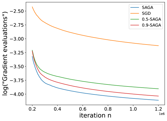
Figure 1: Convergence with $\gamma_{n}=1/n$ for $1.2$M of iterations. Here we put “Gradient evaluations” since instead of using $\|\nabla f(X_{n})\|$, we use the norm of the mean associated to the lines in the matrix $g_{n}$, $\|\sum_{k=1}^{N}g_{n,k}\|/N$. This quantity keeps track of the convergence since it also converges to 0 and its lines converge to the gradients of the functions $f_{k}$, that is for each $1\leqslant k\leqslant N$, $\lim g_{n,k}=\nabla f_{k}(x^{*})$ as $n$ goes to infinity.

Moreover, to illustrate the asymptotic normality result, we use $N=100$, the first $100$ images in the MNIST dataset, and the distributional convergence

$$\lim_{n\rightarrow\infty}\mathds{E}(h(\sqrt{n}(X_{n}-x^{*}))))=\mathds{E}(h(\mathcal{N}_{d}(0,\Sigma))),$$

where $h$ is defined, for all $x\in\mathds{R}^{d}$, by $h(x)={\displaystyle\sum_{i=1}^{d}{x_{i}}}$. It follows from Theorem 2 that

$$h(\sqrt{n}(X_{n}-x^{*})))\quad\overset{\mathcal{L}}{\underset{n\to+\infty}{\longrightarrow}}\quad\mathcal{N}(0,\sigma^{2}(\lambda)).$$

As the equilibrium point $x^{*}$ and the asymptotic variance $\sigma^{2}(\lambda)$ are unknown, we use estimators from the standard Monte Carlo procedure. We denote for each fixed lambda $\widehat{\sigma}^{\,2}_{n}(\lambda)$ the estimator of $\sigma^{2}(\lambda)$. Given the form of our function $h$, we deduce that the limiting variances should be related as $(1-\lambda)^{2}\sigma^{2}(0)=\sigma^{2}(\lambda)$. The results are shown in Figure 2.

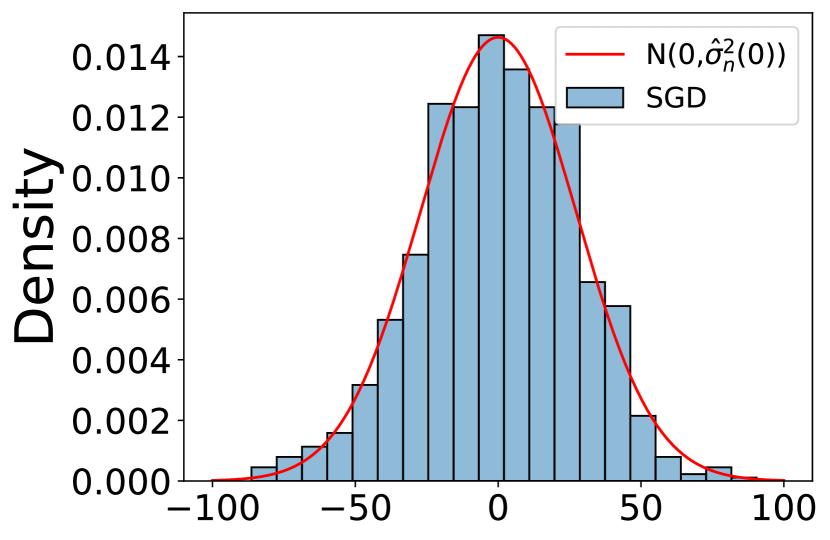
((a)) SGD $(\lambda=0)$, where $\sigma_{n}^{2}(0)\approx 743.11$

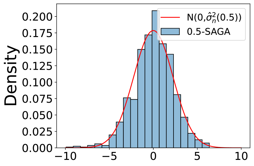
((b)) $0.5$-SAGA, where $\sigma_{n}^{2}(0.5)\approx 5$

((c)) $0.9$-SAGA, where $\sigma_{n}^{2}(0.9)\approx 0.884$

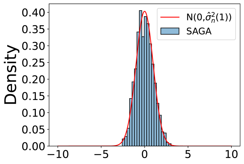
((d)) SAGA ($\lambda=1$), where $\sigma_{n}^{2}(1)\approx 0.98$

Figure 2: We used 1000 samples, where each one was obtained by running the associated algorithm for $n=500000$ iterations.

The main purpose of this plot is to represent the decreasing behavior of the variance with respect to the parameter $\lambda$. Even though for the SAGA ($\lambda=1$) we know that its variance converges to zero, for finite $n$ we can only see that it is shrinking with respect to $n$ to obtain at the limit a Dirac mass at 0. Here, the sample variances satisfy $\hat{\sigma}_{n}^{2}(0.9)<\hat{\sigma}_{n}^{2}(1)$. Nevertheless, they are still very close in the scale of the sample variance $\hat{\sigma}_{n}^{2}(0)$ of the SGD. We explain this as a consequence of the approximations and the fact that the models $\lambda=0.9$ and $\lambda=1$ are intimately related.

Finally, we present approximate results of the mean squared error $\mathds{E}[\|X_{n}-x^{*}\|^{2}]$. For that purpose, we suppose that Assumption 5 is satisfied so that Theorem 3 holds. We run each algorithm for $100$ epochs, where each epoch consists of $1000$ iterations. In order to approximate the expectation, we apply the standard Monte Carlo procedure with $1000$ samples. Here, the approximation of $x^{*}$ is the result of running the SAGA algorithm for $40M$ iterations. The results are illustrated in Figure 3. The plot just give an intuition on the behavior of the mean squared error, since the constant $K$ in Theorem 3 is unknown.

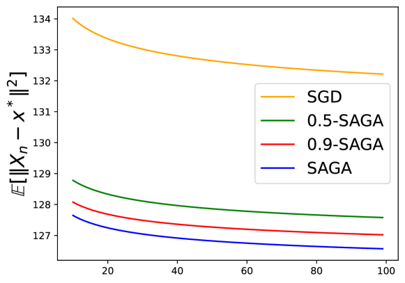
Figure 3: Mean squared error with respect to epochs. We confirm the decreasing order of the mean squared error of $X_{n}-x^{*}$ with respect to $\lambda$ and $n$.

6 Conclusion

Stochastic optimization is one of the main challenges of machine learning touching almost every aspect of the discipline. Thus, in order to meet expectations, the SGD algorithm has been studied at length. However, the advent of Big Data for model learning led to the development of more sophisticated stochastic methods. In our study, we therefore highlight the properties of the new $\lambda$-SAGA algorithm which is a generalization of the SAGA algorithm. We were able to establish the almost sure convergence and the asymptotic normality of this novel algorithm by using a decreasing step and without the strong convexity and Lipschitz gradient assumptions. The other major contribution of our paper concerns the convergence rates in $\mathbf{L}^{p}$ of the $\lambda$-SAGA algorithm. Finally, stochastic algorithms offer multiple guarantees in terms of convergence and certainly promise to continue to have profound impacts on the fast development of the machine learning field.

Acknowledgments and Disclosure of Funding

This project has benefited from state support managed by the Agence Nationale de la Recherche (French National Research Agency) under the reference ANR-20-SFRI-0001.

Appendix A Some useful existing results

We first recall the well-known Robbins-Siegmund Theorem (Robbins and Siegmund, 1971).

Theorem A.1 (Robbins-Siegmund theorem).

Let $(V_{n}),(a_{n}),(\mathcal{A}_{n}),(\mathcal{B}_{n})$ be four positive sequences of random variables adapted to a filtration $(\mathcal{F}_{n})$ such that

$$\mathds{E}[V_{n+1}|\mathcal{F}_{n}]\leqslant(1+a_{n})V_{n}+\mathcal{A}_{n}-\mathcal{B}_{n},$$

where

$$\sum_{n=1}^{\infty}a_{n}<+\infty\qquad\text{and}\qquad\sum_{n=1}^{\infty}\mathcal{A}_{n}<+\infty\qquad a.s.$$

Then, $(V_{n})$ converges almost surely towards a finite random variable $V$ and

$$\sum_{n=1}^{\infty}\mathcal{B}_{n}<+\infty\qquad a.s.$$

The next two lemma provide very useful inequality for non-asymptotic convergence rates. The first lemma is given by Lemma A.3 in supplementary material of Bercu and Bigot (2021), see also Theorem 1 in Bach and Moulines (2011).

Lemma A.1.

(Bercu and Bigot, 2021). Let $(Z_{n})$ be a sequence of positive real numbers satisfying, for all $n\geqslant 1$, the recursive inequality

$$Z_{n+1}\leqslant\left(1-\dfrac{a}{(n+1)^{\alpha}}\right)Z_{n}+\dfrac{b}{(n+1)^{\beta}},$$ (26)

where $a,b,\alpha$ and $\beta$ are positive constants satisfying $a\leqslant 2^{\alpha}$, $\alpha\leqslant 1$, $1<\beta<2$ and $\beta\leqslant 2\alpha$ with $\beta<a+1$ in the special case where $\alpha=1$. Then, there exists a positive constant $C$ such that, for any $n\geqslant 1$,

$$Z_{n}\leqslant\dfrac{C}{n^{\beta-\alpha}}.$$ (27)

The second lemma is given without proof in Chen et al. (2024) in the special case $p\in(0,2]$, see Lemma B.3 as well as the seminal paper Assouad (1975). We extend it to the case $p$ even and we propose a short proof for the sake of completeness.

Lemma A.2.

Let $p$ be a positive even integer . It exist two positive constant $C_{p}$ and $D_{p}$ such that for any $a,\,b\in\mathds{R}^{d}$,

$$\lVert a+b\rVert^{2+p}\leqslant\lVert a\rVert^{2+p}+(2+p)\langle a,b\rangle\lVert a\rVert^{p}+C_{p}\lVert a\rVert^{p}\lVert b\rVert^{2}+D_{p}\lVert b\rVert^{2+p}.$$ (28)

Proof  We prove Lemma A.2 by induction. For the base case $p=2$, we have

$$\lVert a+b\rVert^{4} =\left(\lVert a\rVert^{2}+2\langle a,b\rangle+\lVert b\rVert^{2}\right)^{2}$$

$$=\lVert a\rVert^{4}+4(\langle a,b\rangle)^{2}+\lVert b\rVert^{4}+4\langle a,b\rangle\lVert a\rVert^{2}+4\langle a,b\rangle\lVert b\rVert^{2}+2\lVert a\rVert^{2}\lVert b\rVert^{2}.$$

It follows from Cauchy–Schwarz inequality that $(\langle a,b\rangle)^{2}\leqslant\lVert a\rVert^{2}\lVert b\rVert^{2}$. Moreover, we also have $2\langle a,b\rangle\leqslant\lVert a\rVert^{2}+\lVert b\rVert^{2}$ which implies that $4\langle a,b\rangle\lVert b\rVert^{2}\leqslant 2\lVert a\rVert^{2}\lVert b\rVert^{2}+2\lVert b\rVert^{4}$. Hence, we obtain from these two inequalities that

$$\lVert a+b\rVert^{4}\leqslant\lVert a\rVert^{4}+4\langle a,b\rangle\lVert a\rVert^{2}+8\lVert a\rVert^{2}\lVert b\rVert^{2}+3\lVert b\rVert^{4},$$

which leads to $C_{2}=8$ and $D_{2}=3$. Hereafter, assume that inequality (28) holds up to $q\geq 2$ and let $p=2+q$. We have by induction

$$\lVert a+b\rVert^{2+p}=\lVert a+b\rVert^{2}\lVert a+b\rVert^{p}=\lVert a+b\rVert^{2}\lVert a+b\rVert^{2+q}$$

$$\leqslant\Big{(}\lVert a\rVert^{2}+2\langle a,b\rangle+\lVert b\rVert^{2}\Big{)}\Big{(}\lVert a\rVert^{2+q}+(2+q)\langle a,b\rangle\lVert a\rVert^{q}+C_{q}\lVert a\rVert^{q}\lVert b\rVert^{2}+D_{q}\lVert b\rVert^{2+q}\Big{)}$$

$$\leqslant\lVert a\rVert^{2+p}+(2+p)\langle a,b\rangle\lVert a\rVert^{p}+(C_{q}+2p+1)\lVert a\rVert^{p}\lVert b\rVert^{2}+(2C_{q}+p)\|a\|^{q+1}\|b\|^{3}$$

$$+D_{q}\|a\|^{2}\|b\|^{p}+C_{q}\|a\|^{q}\|b\|^{4}+2D_{q}\|a\|\|b\|^{p+1}+D_{q}\lVert b\rVert^{2+p}$$

where the last inequality is the result of applying Cauchy-Schwarz inequality $\langle a,b\rangle\leq\|a\|\|b\|$ for all the terms multiplied by $\langle a,b\rangle$ but the ones isolated in the second term. Furthermore, it follows from Young’s inequality for products that

$$\|a\|^{q+1}\|b\|^{3}=\|a\|^{q+1}\|b\|^{2(q+1)/p}\times\|b\|^{3-2(q+1)/p} \leq\frac{\|a\|^{p}\|b\|^{2}}{p/(p-1)}+\frac{\|b\|^{p+2}}{p},$$

$$\|a\|^{2}\|b\|^{p}=\|a\|^{2}\|b\|^{4/p}\times\|b\|^{p-4/p} \leq\frac{\|a\|^{p}\|b\|^{2}}{p/2}+\frac{\|b\|^{p+2}}{p/q},$$

$$\|a\|^{q}\|b\|^{4}=\|a\|^{q}\|b\|^{2q/p}\times\|b\|^{4-2q/p} \leq\frac{\|a\|^{p}\|b\|^{2}}{p/q}+\frac{\|b\|^{p+2}}{p/2},$$

$$\|a\|\|b\|^{p+1}=\|a\|\|b\|^{2/p}\times\|b\|^{p+1-2/p} \leq\frac{\|a\|^{p}\|b\|^{2}}{p}+\frac{\|b\|^{p+2}}{p/(p-1)}.$$

Finally, we obtain (28) with $C_{p}$ and $D_{p}$ satisfying the system defined, for $p\geqslant 4$, by

$$\left\{\begin{array}[]{ccc}C_{p}&=&\displaystyle{3p+\frac{4}{p}\Bigl{(}(p-1)C_{p-2}+D_{p-2}\Big{)}\vspace{1ex}}\\ D_{p}&=&\displaystyle{1+\frac{4}{p}\Big{(}C_{p-2}+(p-1)D_{p-2}\Big{)}}\end{array}\right.$$

with initial values $C_{2}=8$ and $D_{2}=3$, which achieves the proof of Lemma A.2.  

Remark A.1.

One can easily compute $C_{4}=39$ and $D_{4}=18$. Moreover, one can observe that we always have $D_{p}\leqslant C_{p}$. Consequently, we can make use of (28) with $C_{p}$ instead of $D_{p}$.

Appendix B Proof of Theorem 2

Proof  The $\lambda$-SAGA algorithm can be rewritten as

$$X_{n+1}=X_{n}-\gamma_{n}(\nabla f(X_{n})+\varepsilon_{n+1}),$$

where $\varepsilon_{n+1}=\mathcal{Y}_{n+1}-\lambda Z_{n+1}$ with

$$\left\{\begin{array}[]{rl}\mathcal{Y}_{n+1}&=\nabla f_{U_{n+1}}(X_{n})-\nabla f(X_{n}),\vspace{0.3cm}\\ Z_{n+1}&=\nabla f_{U_{n+1}}(\phi_{n,U_{n+1}})-\dfrac{1}{N}{\displaystyle\sum_{k=1}^{N}}\nabla f_{k}(\phi_{n,k}).\end{array}\right.$$

We already saw that $(\varepsilon_{n})$ is a martingale difference adapted to the filtration $(\mathcal{F}_{n})$. Moreover,

$$\mathds{E}[\varepsilon_{n+1}\varepsilon_{n+1}^{T}|\mathcal{F}_{n}] =\mathds{E}[\mathcal{Y}_{n+1}\mathcal{Y}_{n+1}^{T}|\mathcal{F}_{n}]-\lambda\mathds{E}[\mathcal{Y}_{n+1}Z_{n+1}^{T}|\mathcal{F}_{n}]-\lambda\mathds{E}[Z_{n+1}\mathcal{Y}_{n+1}^{T}|\mathcal{F}_{n}]$$

$$\hskip 8.5359pt+\lambda^{2}\mathds{E}[Z_{n+1}Z_{n+1}^{T}|\mathcal{F}_{n}].$$

In addition, we clearly have that almost surely

$$\mathds{E}[\mathcal{Y}_{n+1}\mathcal{Y}_{n+1}^{T}|\mathcal{F}_{n}] =\dfrac{1}{N}\sum_{k=1}^{N}\nabla f_{k}(X_{n})\left(\nabla f_{k}(X_{n})\right)^{T}-\nabla f(X_{n})\left(\nabla f(X_{n})\right)^{T},$$

$$\mathds{E}[Z_{n+1}Z_{n+1}^{T}|\mathcal{F}_{n}] =\dfrac{1}{N}\sum_{k=1}^{N}\nabla f_{k}(\phi_{n,k})\left(\nabla f_{k}(\phi_{n,k})\right)^{T}-\dfrac{1}{N^{2}}\left(\sum_{k=1}^{N}\nabla f_{k}(\phi_{n,k})\right)\left(\sum_{k=1}^{N}\left(\nabla f_{k}(\phi_{n,k})\right)^{T}\right),$$

$$\mathds{E}[Z_{n+1}\mathcal{Y}_{n+1}^{T}|\mathcal{F}_{n}] =\dfrac{1}{N}\sum_{k=1}^{N}\nabla f_{k}(\phi_{n,k})\left(\nabla f_{k}(X_{n})\right)^{T}-\dfrac{1}{N}\sum_{k=1}^{N}\nabla f_{k}(\phi_{n,k})\left(\nabla f(X_{n})\right)^{T}.$$

We now claim that for all $1\leqslant k\leqslant N$

$$\lim_{n\to+\infty}\phi_{n,k}=x^{*}\qquad a.s.$$ (29)

As a matter of fact, for a fixed value $1\leqslant k\leqslant N$, the probability that $U_{n}=k$ occurs for infinitely many $n$. Consequently, $(\phi_{n,k})$ is a sub-sequence of $(X_{n})$, since $\phi_{n,k}$ is updated to $X_{n}$ each time $\{U_{n}=k\}$. Hence, the almost sure convergence (29) follows from (19). Combining the almost sure convergence of $(X_{n})$ and $(\phi_{n,k})$ towards $x^{*}$ with the continuity of $\nabla f$ given by Assumption 4, it follows that almost surely

$$\left\{\begin{array}[]{rl}{\displaystyle\lim_{n\to+\infty}}\mathds{E}[\mathcal{Y}_{n+1}\mathcal{Y}_{n+1}^{T}|\mathcal{F}_{n}]&=\Gamma,\vspace{0.2cm}\\ {\displaystyle\lim_{n\to+\infty}}\mathds{E}[\mathcal{Y}_{n+1}Z_{n+1}^{T}|\mathcal{F}_{n}]&=\Gamma,\vspace{0.2cm}\\ {\displaystyle\lim_{n\to+\infty}}\mathds{E}[Z_{n+1}\mathcal{Y}_{n+1}^{T}|\mathcal{F}_{n}]&=\Gamma,\vspace{0.2cm}\\ {\displaystyle\lim_{n\to+\infty}}\mathds{E}[Z_{n+1}Z_{n+1}^{T}|\mathcal{F}_{n}]&=\Gamma,\end{array}\right.$$

where

$$\Gamma=\dfrac{1}{N}\sum_{k=1}^{N}\nabla f_{k}(x^{*})\left(\nabla f_{k}(x^{*})\right)^{T},$$

which leads to

$$\lim_{n\to+\infty}\mathds{E}[\varepsilon_{n+1}\varepsilon_{n+1}^{T}\lvert\mathcal{F}_{n}]=(1-\lambda)^{2}\Gamma\qquad a.s.$$

Therefore, we obtain from Toeplitz’s lemma that

$$\lim_{n\to+\infty}\dfrac{1}{n}\sum_{k=1}^{n}\mathds{E}[\varepsilon_{k}\varepsilon_{k}^{T}\lvert\mathcal{F}_{k-1}]=(1-\lambda)^{2}\Gamma\qquad a.s.$$

In addition, we have for all $n\geqslant 1$

$$\lVert\varepsilon_{n+1}\rVert\leqslant 2\left(\max_{k=1,\dots,N}\lVert\nabla f_{k}(X_{n})\rVert+\lambda\max_{k=1,\dots,N}\lVert\nabla f_{k}(\phi_{n,k})\rVert\right).$$ (30)

Hence, it follows from (30) that

$$\lVert\varepsilon_{n+1}\rVert^{4}\leqslant 128\left(\max_{k=1,\dots,N}\lVert\nabla f_{k}(X_{n})\rVert^{4}+\lambda^{4}\max_{k=1,\dots,N}\lVert\nabla f_{k}(\phi_{n,k})\rVert^{4}\right).$$ (31)

However, for all $k=1,...,N$, we have

$$\lVert\nabla f_{k}(X_{n})\rVert^{2}\leqslant 2\lVert\nabla f_{k}(X_{n})-\nabla f_{k}(x^{*})\rVert^{2}+2\lVert\nabla f_{k}(x^{*})\lVert^{2},$$

which implies that

$$\max_{k=1,\dots,N}\lVert\nabla f_{k}(X_{n})\rVert^{2}\leqslant 2N\Big{(}\tau^{2}(X_{n})+\theta^{*}\Big{)}.$$

Consequently,

$$\max_{k=1,\dots,N}\lVert\nabla f_{k}(X_{n})\rVert^{4}\leqslant 4N^{2}\Big{(}\tau^{2}(X_{n})+\theta^{*}\Big{)}^{2}.$$ (32)

By the same token,

$$\max_{k=1,\dots,N}\lVert\nabla f_{k}(\phi_{n,k})\rVert^{4}\leqslant 4N^{2}\Big{(}A_{n}+\theta^{*}\Big{)}^{2}.$$ (33)

Hence, we obtain from (31), (32) and (33) that

$$\lVert\varepsilon_{n+1}\rVert^{4}\leqslant 512N^{2}\Bigg{(}\Big{(}\tau^{2}(X_{n})+\theta^{*}\Big{)}^{2}+\lambda^{4}\Big{(}A_{n}+\theta^{*}\Big{)}^{2}\Bigg{)},$$

which immediately implies that

$$\mathds{E}[\lVert\varepsilon_{n+1}\rVert^{4}|\mathcal{F}_{n}]\leqslant 512N^{2}\Bigg{(}\Big{(}\tau^{2}(X_{n})+\theta^{*}\Big{)}^{2}+\lambda^{4}\Big{(}A_{n}+\theta^{*}\Big{)}^{2}\Bigg{)}\qquad a.s.$$ (34)

Moreover, since $X_{n}$ converges towards $x^{*}$, it follows that $\tau^{2}(X_{n})$ converges to 0 almost surely. Combining this result with the almost sure convergence of $A_{n}$ towards 0 and (34), we find that

$$\sup_{n\geqslant 1}\mathds{E}[\lVert\varepsilon_{n+1}\rVert^{4}\lvert\mathcal{F}_{n}]<+\infty,$$

which implies that for all $\epsilon>0$,

$$\lim_{n\to+\infty}\dfrac{1}{n}\sum_{k=1}^{n}\mathds{E}\left[\lVert\varepsilon_{k}\rVert^{2}\mathds{1}_{\{\lVert\varepsilon_{k}\rVert\geqslant\epsilon\sqrt{n}\}}\lvert\mathcal{F}_{k-1}\right]=0\qquad a.s.$$

Finally, it follows from the central limit theorem for stochastic algorithms given by Theorem 2.3 in (Zhang, 2016) that

$$\sqrt{n}(X_{n}-x^{*})\quad\overset{\mathcal{L}}{\underset{n\to+\infty}{\longrightarrow}}\quad\mathcal{N}_{d}(0,\Sigma),$$

where

$$\Sigma=(1-\lambda)^{2}\int_{0}^{\infty}(e^{-(H-\mathds{I}_{d}/2)u})^{T}\Gamma e^{-(H-\mathds{I}_{d}/2)u}du,$$

which completes the proof of Theorem 2.  

Appendix C Proof of Theorem 3

Proof  We already saw in (13) that for all $n\geq 1$,

$$\mathds{E}[V_{n+1}|\mathcal{F}_{n}]\leqslant V_{n}-2\gamma_{n}\langle X_{n}-x^{*},\nabla f(X_{n})\rangle+3\gamma_{n}^{2}\big{(}\tau^{2}(X_{n})+A_{n}+\theta^{*}\big{)}\qquad a.s.$$

Hence, it follows from Assumption 5 that $\langle X_{n}-x^{*},\nabla f(X_{n})\rangle\geqslant\mu V_{n}$, which leads to

$$\mathds{E}[V_{n+1}|\mathcal{F}_{n}]\leqslant(1-2\mu\gamma_{n})V_{n}+3\gamma_{n}^{2}\big{(}\tau^{2}(X_{n})+A_{n}+\theta^{*}\big{)}\qquad a.s.$$

By taking the expectation on both side of this inequality, we obtain that for all $n\geq 1$,

$$\mathds{E}[V_{n+1}]\leqslant(1-2\mu\gamma_{n})\mathds{E}[V_{n}]+3\gamma_{n}^{2}\big{(}\mathds{E}[\tau^{2}(X_{n})]+\mathds{E}[A_{n}]+\theta^{*}\big{)}.$$ (35)

Furthermore, we deduce from Corollary 7 in Appendix E below that there exist positive constants $b_{1}$ and $b_{2}$ such that, for all $n\geqslant 1$, $\mathds{E}[\tau^{2}(X_{n})]\leqslant b_{1}$ and $\mathds{E}[A_{n}]\leqslant b_{2}$. Consequently, (35) immediately leads, for all $n\geqslant 1$, to

$$\mathds{E}[V_{n+1}]\leqslant\left(1-\frac{a}{(n+1)^{\alpha}}\right)\mathds{E}[V_{n}]+\frac{b}{(n+1)^{2\alpha}}$$

where $a=2\mu c$ and $b=3c^{2}4^{\alpha}(b_{1}+b_{2}+\theta^{*})$. Finally, we can conclude from Lemma A.1 that there exists a positive constant $K$ such that for any $n\geqslant 1$,

$$\mathds{E}[\lVert X_{n}-x^{*}\rVert^{2}]\leqslant\dfrac{K}{n^{\alpha}},$$

which completes the proof of Theorem 3.  

Appendix D Proof of Theorem 4

Proof  First of all, Theorem 4 follows from Theorem 3 in the special case $p=1$. Hence, we are going to prove Theorem 4 by induction on $n\geqslant 1$ for some integer $p\geqslant 2$ satisfying Assumption 6. As the initial state $X_{1}$ belongs to $\mathbf{L}^{2p}$, the base case is immediately true. Next, assume by induction that for some integer $m$ which will be fixed soon, there exists a positive constant $K_{p}$ such that for all $n\leqslant m$,

$$\mathds{E}[\lVert X_{n}-x^{*}\rVert^{2p}]\leqslant\dfrac{K_{p}}{n^{p\alpha}}.$$ (36)

We have from (6) together with Lemma A.2 that it exists a positive constant $C_{p}$ such that for all $n\geqslant 1$,

$$V_{n+1}^{p} =\lVert X_{n+1}-x^{*}\rVert^{2p},$$

$$=\lVert X_{n}-x^{*}-\gamma_{n}(Y_{n+1}-\lambda Z_{n+1})\rVert^{2p},$$

$$\leqslant V_{n}^{p}-2p\gamma_{n}V_{n}^{p-1}\langle X_{n}-x^{*},Y_{n+1}-\lambda Z_{n+1}\rangle+C_{p}\gamma_{n}^{2}V_{n}^{p-1}\lVert Y_{n+1}-\lambda Z_{n+1}\rVert^{2}$$

$$+C_{p}\gamma_{n}^{2p}\lVert Y_{n+1}-\lambda Z_{n+1}\rVert^{2p}.$$

Hence, it follows from (7) that

$$\mathds{E}[V_{n+1}^{p}|\mathcal{F}_{n}] \leqslant V_{n}^{p}-2p\gamma_{n}V_{n}^{p-1}\langle X_{n}-x^{*},\nabla f(X_{n})\rangle$$ (37)

$$+C_{p}\gamma_{n}^{2}V_{n}^{p-1}\mathds{E}[\lVert Y_{n+1}-\lambda Z_{n+1}\rVert^{2}|\mathcal{F}_{n}]+C_{p}\gamma_{n}^{2p}\mathds{E}[\lVert Y_{n+1}-\lambda Z_{n+1}\rVert^{2p}|\mathcal{F}_{n}].$$

We already saw from (12) that

$$\mathds{E}[\lVert Y_{n+1}-\lambda Z_{n+1}\rVert^{2}|\mathcal{F}_{n}]\leqslant 3\big{(}\tau^{2}(X_{n})+A_{n}+\theta^{*}\big{)}\qquad a.s.$$

which leads, via Assumption 6, to

$$\mathds{E}[\lVert Y_{n+1}-\lambda Z_{n+1}\rVert^{2}|\mathcal{F}_{n}]\leqslant 3\big{(}L_{p}^{1/p}\,V_{n}+A_{n}+\theta^{*}\big{)}\qquad a.s.$$

Moreover, as in the proof of (8), we deduce from Jensen’s inequality that

$$\mathds{E}[\lVert Y_{n+1}-\lambda Z_{n+1}\rVert^{2p}|\mathcal{F}_{n}]\leqslant 3^{2p-1}\mathds{E}[\lVert Y_{n+1}-\nabla f_{U_{n+1}}(x^{*})\rVert^{2p}|\mathcal{F}_{n}]$$ (38)

$$+3^{2p-1}\mathds{E}[\lVert Z_{n+1}-\nabla f_{U_{n+1}}(x^{*})\rVert^{2p}|\mathcal{F}_{n}]+3^{2p-1}\mathds{E}[\lVert\nabla f_{U_{n+1}}(x^{*})\rVert^{2p}|\mathcal{F}_{n}].$$

Hereafter, we clearly have

$$\mathds{E}[\lVert\nabla f_{U_{n+1}}(x^{*})\rVert^{2p}|\mathcal{F}_{n}]=\dfrac{1}{N}\sum_{k=1}^{N}\lVert\nabla f_{k}(x^{*})\rVert^{2p}\qquad a.s.$$ (39)

Moreover, denote

$$A_{p,n}=\dfrac{1}{N}\sum_{k=1}^{N}\lVert\nabla f_{k}(\phi_{n,k})-\nabla f_{k}(x^{*})\rVert^{2p}\qquad\text{and}\qquad\Sigma_{n}=\dfrac{1}{N}\sum_{k=1}^{N}\nabla f_{k}(\phi_{n,k}).$$

It follows once again from Jensen’s inequality that

$$\mathds{E}[\lVert Z_{n+1}-\nabla f_{U_{n+1}}(x^{*})\rVert^{2p}|\mathcal{F}_{n}]\leqslant 2^{2p-1}\big{(}A_{p,n}+\left\lVert\Sigma_{n}\right\rVert^{2p}\big{)}\qquad a.s.$$ (40)

However, we obtain from Holder’s inequality that $\left\lVert\Sigma_{n}\right\rVert^{2p}\leqslant A_{p,n}$. Consequently, inequality (40) immediately leads to

$$\mathds{E}[\lVert Z_{n+1}-\nabla f_{U_{n+1}}(x^{*})\rVert^{2p}|\mathcal{F}_{n}]\leqslant 4^{p}A_{p,n}\qquad a.s.$$ (41)

Furthermore, define for all $x\in\mathds{R}^{d}$,

$$\tau^{2p}(x)=\dfrac{1}{N}\sum_{k=1}^{N}\lVert\nabla f_{k}(x)-\nabla f_{k}(x^{*})\rVert^{2p}.$$

As in the proof of Theorem 1, one can observe that

$$\mathds{E}[\lVert Y_{n+1}-\nabla f_{U_{n+1}}(x^{*})\rVert^{2p}|\mathcal{F}_{n}]=\tau^{2p}(X_{n})\qquad a.s.$$ (42)

Putting together the three contributions (39), (41) and (42), we obtain from (38) that

$$\mathds{E}[\lVert Y_{n+1}-\lambda Z_{n+1}\rVert^{2p}|\mathcal{F}_{n}]\leqslant 3^{2p-1}(\tau^{2p}(X_{n})+4^{p}A_{p,n}+\theta^{*}_{p})\qquad a.s.$$ (43)

where

$$\theta^{*}_{p}=\dfrac{1}{N}\sum_{k=1}^{N}\lVert\nabla f_{k}(x^{*})\rVert^{2p}.$$

Hence, Assumption 6 implies that

$$\mathds{E}[\lVert Y_{n+1}-\lambda Z_{n+1}\rVert^{2p}|\mathcal{F}_{n}]\leqslant 3^{2p-1}(L_{p}V_{n}^{p}+4^{p}A_{p,n}+\theta^{*}_{p})\qquad a.s.$$ (44)

Therefore, we deduce from (37) and (44) that for all $n\geqslant 1$,

$$\mathds{E}[V_{n+1}^{p}|\mathcal{F}_{n}] \leqslant\Big{(}1+3L_{p}^{1/p}\,C_{p}\gamma_{n}^{2}+3^{2p-1}L_{p}C_{p}\gamma_{n}^{2p}\Big{)}V_{n}^{p}$$

$$-2p\gamma_{n}V_{n}^{p-1}\langle X_{n}-x^{*},\nabla f(X_{n})\rangle+3C_{p}\gamma_{n}^{2}V_{n}^{p-1}(A_{n}+\theta^{*})$$

$$+3^{2p-1}C_{p}\gamma_{n}^{2p}(4^{p}A_{p,n}+\theta^{*}_{p})\qquad a.s.$$

Furthermore, it follows from Assumption 5 that $\langle X_{n}-x^{*},\nabla f(X_{n})\rangle\geqslant\mu V_{n}$, which leads to

$$\mathds{E}[V_{n+1}^{p}|\mathcal{F}_{n}] \leqslant\Big{(}1+3L_{p}^{1/p}\,C_{p}\gamma_{n}^{2}+3^{2p-1}L_{p}C_{p}\gamma_{n}^{2p}-2\mu p\gamma_{n}\Big{)}V_{n}^{p}$$

$$+3C_{p}\gamma_{n}^{2}V_{n}^{p-1}(A_{n}+\theta^{*})+3^{2p-1}C_{p}\gamma_{n}^{2p}(4^{p}A_{p,n}+\theta^{*}_{p})\qquad a.s.$$ (45)

By taking the expectation on both side of this inequality, we obtain that for all $n\geq 1$,

$$\mathds{E}[V_{n+1}^{p}] \leqslant\Big{(}1+3L_{p}^{1/p}\,C_{p}\gamma_{n}^{2}+3^{2p-1}L_{p}C_{p}\gamma_{n}^{2p}-2\mu p\gamma_{n}\Big{)}\mathds{E}[V_{n}^{p}]+3C_{p}\gamma_{n}^{2}\mathds{E}[A_{n}V_{n}^{p-1}]$$

$$+3C_{p}\gamma_{n}^{2}\theta^{*}\mathds{E}[V_{n}^{p-1}]+3^{2p-1}C_{p}\gamma_{n}^{2p}(4^{p}\mathds{E}[A_{p,n}]+\theta^{*}_{p})$$ (46)

We deduce from Corollary 9 in Appendix F below that there exists a positive constant $d_{p}$ such that for all $n\geqslant 1$, $\mathds{E}[A_{p,n}]\leqslant d_{p}$. The main difficulty arising here is to find a sharp upper bound for the crossing term $\mathds{E}[A_{n}V_{n}^{p-1}]$. By using once again Holder’s inequality, we have for all $n\geqslant 1$,

$$\mathds{E}[A_{n}V_{n}^{p-1}]\leq\Big{(}\mathds{E}[A_{n}^{p}]\Big{)}^{\frac{1}{p}}\Big{(}\mathds{E}[V_{n}^{p}]\Big{)}^{\frac{p-1}{p}}\qquad\text{and}\qquad\mathds{E}[V_{n}^{p-1}]\leq\Big{(}\mathds{E}[V_{n}^{p}]\Big{)}^{\frac{p-1}{p}}.$$ (47)

Hence, it is necessary to compute an upper bound for $\mathds{E}[A_{n}^{p}]$. Nevertheless, one can observe from Jensen’s inequality that we always have $A_{n}^{p}\leqslant A_{p,n}$, which leads that $\mathds{E}[A_{n}^{p}]\leqslant d_{p}$. Therefore, it follows from the induction hypothesis (36) together with (D) and (47) that

$$\mathds{E}[V_{n+1}^{p}]\leqslant\Big{(}1+\xi_{n}-2\mu p\gamma_{n}\Big{)}\mathds{E}[V_{n}^{p}]+\frac{b}{(n+1)^{\alpha(p+1)}}$$ (48)

where $\xi_{n}=3L_{p}^{1/p}\,C_{p}\gamma_{n}^{2}+3^{2p-1}L_{p}C_{p}\gamma_{n}^{2p}$ and

$$b=2^{\alpha(p+1)}c^{2}C_{p}\Big{(}3K_{p}^{(p-1)/p}\big{(}d_{p}^{1/p}+\theta^{*}\big{)}+c^{p-1}3^{2p-1}\big{(}4^{p}d_{p}+\theta_{p}^{*}\big{)}\Big{)}.$$

Hereafter, denote by $m$ the integer part of the real number

$$\Bigl{(}\frac{3cC_{p}}{\mu p}\Bigr{)}^{1/\alpha}\Big{(}L_{p}^{1/p}+3^{2(p-1)}\Big{)}^{1/\alpha}.$$

One can easily check that as soon as $n\geqslant m$, $\xi_{n}\leq\mu p\gamma_{n}$. Consequently, we find from (48) that as soon as $n\geqslant m$,

$$\mathds{E}[V_{n+1}^{p}]\leqslant\left(1-\frac{a}{(n+1)^{\alpha}}\right)\mathds{E}[V_{n}^{p}]+\frac{b}{(n+1)^{\alpha(p+1)}}$$ (49)

where $a=p\mu c$. Finally, we deduce from Lemma A.1 that there exists a positive constant $K_{p}$ such that for all $n\geqslant 1$,

$$\mathds{E}[\lVert X_{n+1}-x^{*}\rVert^{2p}]\leqslant\dfrac{K_{p}}{(n+1)^{\alpha p}},$$

which achieves the induction on $n$ and completes the proof of Theorem 4.  

Appendix E Additional asymptotic result on the convergence in $\mathbf{L}^{2}$

The goal of this appendix is to provide additional asymptotic properties of the $\lambda$-SAGA algorithm that will be useful in the proofs of our main results. First of all, we recall that $V_{n}=\lVert X_{n}-x^{*}\rVert^{2}$,

$$A_{n}=\dfrac{1}{N}{\displaystyle\sum_{k=1}^{N}}\lVert\nabla f_{k}(\phi_{n,k})-\nabla f_{k}(x^{*})\rVert^{2}\quad\text{and}\quad\tau^{2}(x)=\dfrac{1}{N}{\displaystyle\sum_{k=1}^{N}}\lVert\nabla f_{k}(x)-\nabla f_{k}(x^{*})\rVert^{2}.$$

Theorem 6.

Consider a fixed $\lambda\in[0,1]$. Let $(X_{n})$ be the sequence generated by the $\lambda$-SAGA algorithm with decreasing step sequence $(\gamma_{n})$ satisfying (2). Suppose that Assumptions 1, 3 and 5 are satisfied. Then, we have almost surely

$$\sum_{n=1}^{\infty}\gamma_{n}V_{n}<+\infty,\qquad\sum_{n=1}^{\infty}\gamma_{n}A_{n}<+\infty,\qquad\sum_{n=1}^{\infty}\gamma_{n}\tau^{2}(X_{n})<+\infty.$$ (50)

In addition, we also have

$$\sum_{n=1}^{\infty}\gamma_{n}\mathds{E}[V_{n}]<+\infty,\qquad\sum_{n=1}^{\infty}\gamma_{n}\mathds{E}[A_{n}]<+\infty,\qquad\sum_{n=1}^{\infty}\gamma_{n}\mathds{E}[\tau^{2}(X_{n})]<+\infty.$$ (51)

Proof  Let us consider the same Lyapounov function used in the proof of Theorem 1 and given by (14). We recall from inequality (17) that for all $n\geqslant 1$,

$$\mathds{E}[T_{n+1}|\mathcal{F}_{n}]\leqslant(1+6L\gamma_{n}^{2})T_{n}-2\gamma_{n}\langle X_{n}-x^{*},\nabla f(X_{n})\rangle+3\theta^{*}\gamma_{n}^{2}\qquad a.s.$$ (52)

Let $(\mathcal{T}_{n})$ be the sequence of Lyapunov functions defined, for all $n\geqslant 2$, by $\mathcal{T}_{n}=b_{n}T_{n}$ where

$$b_{n}=\prod_{k=1}^{n-1}\big{(}1+6L\gamma_{k}^{2}\big{)}^{-1}.$$

Since $b_{n}=b_{n+1}(1+6L\gamma_{n}^{2})$, we obtain from (52) that for all $n\geqslant 1$,

$$\mathds{E}[\mathcal{T}_{n+1}|\mathcal{F}_{n}]\leqslant\mathcal{T}_{n}-2\gamma_{n}b_{n+1}\langle X_{n}-x^{*},\nabla f(X_{n})\rangle+3\theta^{*}b_{n+1}\gamma_{n}^{2}\qquad a.s.$$

Hence, it follows from Assumption 5 that for all $n\geqslant 1$,

$$\mathds{E}[\mathcal{T}_{n+1}|\mathcal{F}_{n}]\leqslant\mathcal{T}_{n}-2\mu\gamma_{n}b_{n+1}V_{n}+3\theta^{*}b_{n+1}\gamma_{n}^{2}\qquad a.s.$$ (53)

Moreover, we clearly have from the right-hand side of (2) that $(b_{n})$ converges to a positive real number $b$, which implies that

$$\sum_{n=1}^{\infty}b_{n+1}\gamma_{n}^{2}<+\infty.$$ (54)

Therefore, we deduce from the Robbins-Siegmund Theorem (Robbins and Siegmund, 1971) given by Theorem A.1 that $(\mathcal{T}_{n})$ converges almost surely towards a finite random variable $\mathcal{T}$ and the series

$$\sum_{n=2}^{\infty}\gamma_{n}b_{n+1}V_{n}<+\infty\qquad a.s.$$

which leads to

$$\sum_{n=1}^{\infty}\gamma_{n}V_{n}<+\infty\qquad a.s.$$ (55)

We also obtain from relation (55) and Assumption 3 that

$$\sum_{n=1}^{\infty}\gamma_{n}\tau^{2}(X_{n})<+\infty\qquad a.s.$$ (56)

In addition, by taking the expectation of both sides of (53) and using a standard telescoping argument, we find that

$$2\mu\sum_{n=2}^{\infty}\gamma_{n}b_{n+1}\mathds{E}[V_{n}]\leqslant\mathds{E}[\mathcal{T}_{2}]+3\theta^{*}\sum_{n=2}^{\infty}b_{n+1}\gamma_{n}^{2}.$$ (57)

Then, it follows from (54) and (57) that

$$\sum_{n=2}^{\infty}\gamma_{n}b_{n+1}\mathds{E}[V_{n}]<+\infty,$$

which implies that

$$\sum_{n=1}^{\infty}\gamma_{n}\mathds{E}[V_{n}]<+\infty.$$

Consequently, we get from Assumption 3 that

$$\sum_{n=1}^{\infty}\gamma_{n}\mathds{E}[\tau^{2}(X_{n})]<+\infty.$$ (58)

Furthermore, we already saw from (4.1) that for all $n\geqslant 1$,

$$\mathds{E}[A_{n+1}|\mathcal{F}_{n}]=\dfrac{1}{N}\tau^{2}(X_{n})+\left(1-\dfrac{1}{N}\right)A_{n}\qquad a.s.$$ (59)

For all $n\geqslant 1$, denote $\mathcal{A}_{n}=\gamma_{n}A_{n}$. Since $\gamma_{n+1}\leqslant\gamma_{n}$, we obtain from (59) that for all $n\geqslant 1$,

$$\mathds{E}[\mathcal{A}_{n+1}|\mathcal{F}_{n}]\leqslant\mathcal{A}_{n}+\dfrac{1}{N}\gamma_{n}\tau^{2}(X_{n})-\dfrac{1}{N}\gamma_{n}A_{n}\qquad a.s.$$ (60)

By considering the almost sure convergence (56), it follows once again from the Robbins-Siegmund Theorem (Robbins and Siegmund, 1971) given by Theorem A.1 that $(\mathcal{A}_{n})$ converges almost surely towards a finite random variable $\mathcal{A}$ and the series

$$\sum_{n=1}^{\infty}\gamma_{n}A_{n}<+\infty\qquad a.s.$$

Moreover, by taking the expectation of both sides of (60) and using a standard telescoping argument, we obtain that

$$\sum_{n=1}^{\infty}\gamma_{n}\mathds{E}[A_{n}]\leqslant N\mathds{E}[\mathcal{A}_{1}]+\sum_{n=1}^{\infty}\gamma_{n}\mathds{E}[\tau^{2}(X_{n})].$$ (61)

Finally, we deduce from (58) and (61) that

$$\sum_{n=1}^{\infty}\gamma_{n}\mathds{E}[A_{n}]<+\infty,$$

which completes the proof of Theorem 6.  
A straightforward application of Theorem 6, using the left-hand side of (2), is as follows.

Corollary 7.

Assume that the conditions of Theorem 6 hold. Then, we have

$$\lim_{n\to+\infty}V_{n}=\lim_{n\to+\infty}A_{n}=\lim_{n\to+\infty}\tau^{2}(X_{n})=0\qquad a.s.$$

Moreover, we also have

$$\lim_{n\to+\infty}\mathds{E}[V_{n}]=\lim_{n\to+\infty}\mathds{E}[A_{n}]=\lim_{n\to+\infty}\mathds{E}[\tau^{2}(X_{n})]=0.$$

Appendix F Additional asymptotic result on the convergence in $\mathbf{L}^{p}$

As in the previous Appendix, our purpose is to establish additional asymptotic properties of the $\lambda$-SAGA algorithm that will be useful in the proofs of our main results. First of all, we recall that $V_{n}^{p}=\lVert X_{n}-x^{*}\rVert^{2p}$,

$$A_{p,n}=\dfrac{1}{N}{\displaystyle\sum_{k=1}^{N}}\lVert\nabla f_{k}(\phi_{n,k})-\nabla f_{k}(x^{*})\rVert^{2p}\quad\text{and}\quad\tau^{2p}(x)=\dfrac{1}{N}{\displaystyle\sum_{k=1}^{N}}\lVert\nabla f_{k}(x)-\nabla f_{k}(x^{*})\rVert^{2p}.$$

Theorem 8.

Consider a fixed $\lambda\in[0,1]$. Let $(X_{n})$ be the sequence generated by the $\lambda$-SAGA algorithm with decreasing step $\gamma_{n}$ satisfying (2). Suppose that Assumptions 1, 5 and 6 are satisfied. Then, we have almost surely

$$\sum_{n=1}^{\infty}\gamma_{n}V_{n}^{p}<+\infty,\qquad\sum_{n=1}^{\infty}\gamma_{n}A_{p,n}<+\infty,\qquad\sum_{n=1}^{\infty}\gamma_{n}\tau^{2p}(X_{n})<+\infty.$$ (62)

In addition, we also have

$$\sum_{n=1}^{\infty}\gamma_{n}\mathds{E}[V_{n}^{p}]<+\infty,\qquad\sum_{n=1}^{\infty}\gamma_{n}\mathds{E}[A_{p,n}]<+\infty,\qquad\sum_{n=1}^{\infty}\gamma_{n}\mathds{E}[\tau^{2p}(X_{n})]<+\infty.$$ (63)

Proof  We are going to prove Theorem 8 by induction on $p\geqslant 1$. First of all, Theorem 8 follows from Theorem 6 in the special case $p=1$. Hence, the base case is immediately true. Next, assume by induction that Theorem 8 holds for some integer $p-1$ with $p\geqslant 2$. We recall from inequality (D) in the proof of Theorem 4 that for all $n\geqslant 1$,

$$\mathds{E}[V_{n+1}^{p}|\mathcal{F}_{n}] \leqslant\Big{(}1+3L_{p}^{1/p}\,C_{p}\gamma_{n}^{2}+3^{2p-1}L_{p}C_{p}\gamma_{n}^{2p}-2\mu p\gamma_{n}\Big{)}V_{n}^{p}$$

$$+3C_{p}\gamma_{n}^{2}V_{n}^{p-1}(A_{n}+\theta^{*})+3^{2p-1}C_{p}\gamma_{n}^{2p}(4^{p}A_{p,n}+\theta^{*}_{p})\qquad a.s.$$ (64)

However, it follows from Young’s inequality for products that almost surely

$$V_{n}^{p-1}A_{n}\leqslant\dfrac{A_{n}^{p}}{p}+\dfrac{(p-1)V_{n}^{p}}{p}.$$ (65)

Moreover, one can observe from Jensen’s inequality that $A_{n}^{p}\leqslant A_{p,n}$ almost surely. Combining the previous inequality with (65), it implies that

$$V_{n}^{p-1}A_{n}\leqslant\dfrac{A_{p,n}}{p}+\dfrac{(p-1)V_{n}^{p}}{p}.$$ (66)

Furthermore, by putting together the inequalities (F) and (66), we obtain that

$$\mathds{E}[V_{n+1}^{p}|\mathcal{F}_{n}] \leqslant\left(1+3\big{(}L_{p}^{1/p}+3p^{-1}(p-1)\big{)}C_{p}\gamma_{n}^{2}+3^{2p-1}L_{p}C_{p}\gamma_{n}^{2p}\right)V_{n}^{p}-2\mu p\gamma_{n}V_{n}^{p}$$

$$+3C_{p}\theta^{*}\gamma_{n}^{2}V_{n}^{p-1}+\Big{(}3^{2p-1}4^{p}+3p^{-1}\Big{)}C_{p}\gamma_{n}^{2}A_{p,n}+3^{2p-1}C_{p}\gamma_{n}^{2p}\theta^{*}_{p}\qquad a.s.$$ (67)

Let $(T_{p,n})$ be the sequence of Lyapunov functions defined, for all $n\geqslant 2$, by

$$T_{p,n}=V_{n}^{p}+Ne_{p}\gamma_{n-1}^{2}A_{p,n},$$ (68)

where $e_{p}=3^{2p-1}4^{p}+3p^{-1}$. By the definition (68), we have

$$\mathds{E}[T_{p,n+1}|\mathcal{F}_{n}]=\mathds{E}[V_{n+1}^{p}|\mathcal{F}_{n}]+Ne_{p}\gamma_{n}^{2}\mathds{E}[A_{p,n+1}|\mathcal{F}_{n}]\qquad a.s.$$ (69)

However, we deduce by the same arguments as in (4.1) that

$$\mathds{E}[A_{p,n+1}|\mathcal{F}_{n}]=\dfrac{1}{N}\tau^{2p}(X_{n})+\left(1-\dfrac{1}{N}\right)A_{p,n}\qquad a.s.$$ (70)

Hence, it follows from (F), (69) and (70) that

$$\mathds{E}[T_{p,n+1}|\mathcal{F}_{n}] \leqslant T_{p,n}+3C_{p}\left(\big{(}L_{p}^{1/p}+3p^{-1}(p-1)\big{)}\gamma_{n}^{2}+3^{2(p-1)}L_{p}\gamma_{n}^{2p}\right)V_{n}^{p}-2\mu p\gamma_{n}V_{n}^{p}$$

$$+e_{p}\gamma_{n}^{2}\tau^{2p}(X_{n})+3C_{p}\theta^{*}\gamma_{n}^{2}V_{n}^{p-1}+3^{2p-1}C_{p}\gamma_{n}^{2p}\theta^{*}_{p}\qquad a.s.$$ (71)

Additionally, we clearly have $V_{n}^{p}\leqslant T_{p,n}$ and Assumption 6 leads to

$$\tau^{2p}(X_{n})\leqslant L_{p}V_{n}^{p}\leqslant L_{p}T_{p,n}.$$

Finally, we obtain from (F) that

$$\mathds{E}[T_{p,n+1}|\mathcal{F}_{n}]\leqslant(1+a_{n})T_{p,n}+\Delta_{n}-2\mu p\gamma_{n}V_{n}^{p}\qquad a.s.,$$ (72)

where $\Delta_{n}=3C_{p}\theta^{*}\gamma_{n}^{2}V_{n}^{p-1}+3^{2p-1}C_{p}\gamma_{n}^{2p}\theta^{*}_{p}$ and

$$a_{n}=e_{p}L_{p}\gamma_{n}^{2}+3C_{p}\big{(}L_{p}^{1/p}+3p^{-1}(p-1)\big{)}\gamma_{n}^{2}+3^{2p-1}L_{p}C_{p}\gamma_{n}^{2p}.$$

Since the sequence $(\gamma_{n})$ satisfies (2), it is easy to see that

$$\sum_{n=1}^{\infty}a_{n}<+\infty.$$

Moreover, by the induction hypothesis, we have that

$$\left\{\begin{array}[]{rl}&\displaystyle{\sum_{n=1}^{\infty}}\gamma_{n}V_{n}^{p-1}<+\infty\qquad a.s.,\vspace{1ex}\\ &\displaystyle{\sum_{n=1}^{\infty}}\gamma_{n}\mathds{E}[V_{n}^{p-1}]<+\infty.\end{array}\right.$$ (73)

From (73), one can immediately deduce that

$$\left\{\begin{array}[]{rl}&\displaystyle{\sum_{n=1}^{\infty}}\Delta_{n}<+\infty\qquad a.s.,\vspace{1ex}\\ &\displaystyle{\sum_{n=1}^{\infty}}\mathds{E}[\Delta_{n}]<+\infty.\end{array}\right.$$ (74)

Therefore, one uses exactly the same lines as in the proof of Theorem 6 and the Robbins-Siegmund Theorem (Robbins and Siegmund, 1971) given by Theorem A.1 to show that

$$\left\{\begin{array}[]{rl}&\displaystyle{\sum_{n=1}^{\infty}}V_{n}^{p}<+\infty\qquad a.s.,\vspace{1ex}\\ &\displaystyle{\sum_{n=1}^{\infty}}\mathds{E}[V_{n}^{p}]<+\infty.\end{array}\right.$$ (75)

Hence, combining (75) with Assumption 6, one immediately deduces that

$$\left\{\begin{array}[]{rl}&\displaystyle{\sum_{n=1}^{\infty}}\tau^{2p}(X_{n})<+\infty\qquad a.s.,\vspace{1ex}\\ &\displaystyle{\sum_{n=1}^{\infty}}\mathds{E}[\tau^{2p}(X_{n})]<+\infty.\end{array}\right.$$ (76)

Finally, using once again the same arguments as in the proof of Theorem 6, we obtain that

$$\left\{\begin{array}[]{rl}&\displaystyle{\sum_{n=1}^{\infty}}A_{p,n}<+\infty\qquad a.s.,\vspace{1ex}\\ &\displaystyle{\sum_{n=1}^{\infty}}\mathds{E}[A_{p,n}]<+\infty.\end{array}\right.,$$ (77)

which achieves the proof of Theorem 8.  
A useful consequence of Theorem 8, using the left-hand side of (2), is as follows.

Corollary 9.

Assume that the conditions of Theorem 8 hold. Then, for all $p\geqslant 1$, we have

$$\lim_{n\to+\infty}V_{n}^{p}=\lim_{n\to+\infty}A_{p,n}=\lim_{n\to+\infty}\tau^{2p}(X_{n})=0\qquad a.s.,$$

and

$$\lim_{n\to+\infty}\mathds{E}[V_{n}^{p}]=\lim_{n\to+\infty}\mathds{E}[A_{p,n}]=\lim_{n\to+\infty}\mathds{E}[\tau^{2p}(X_{n})]=0.$$

References

- Allen-Zhu (2018) Zeyuan Allen-Zhu. Katyusha: The first direct acceleration of stochastic gradient methods. Journal of Machine Learning Research, 18(221):1–51, 2018.
- Assouad (1975) P. Assouad. Espaces -lisses et -convexes. Inégalités de Burkholder. Séminaire Maurey-Schwartz, pages 1–7, 1975. talk:15.
- Bach (2014) Francis Bach. Adaptivity of averaged stochastic gradient descent to local strong convexity for logistic regression. The Journal of Machine Learning Research, 15(1):595–627, 2014.
- Bach and Moulines (2011) Francis Bach and Eric Moulines. Non-asymptotic analysis of stochastic approximation algorithms for machine learning. Advances in neural information processing systems, 24, 2011.
- Bercu and Bigot (2021) Bernard Bercu and Jérémie Bigot. Asymptotic distribution and convergence rates of stochastic algorithms for entropic optimal transportation between probability measures. The Annals of Statistics, 49(2):968–987, 2021.
- Bercu et al. (2020) Bernard Bercu, Antoine Godichon, and Bruno Portier. An efficient stochastic Newton algorithm for parameter estimation in logistic regressions. SIAM J. Control Optim., 58(1):348–367, 2020.
- Bertsekas and Tsitsiklis (2000) Dimitri P Bertsekas and John N Tsitsiklis. Gradient convergence in gradient methods with errors. SIAM Journal on Optimization, 10(3):627–642, 2000.
- Bottou et al. (2018) Léon Bottou, Frank E Curtis, and Jorge Nocedal. Optimization methods for large-scale machine learning. SIAM review, 60(2):223–311, 2018.
- Chatterji et al. (2018) Niladri Chatterji, Nicolas Flammarion, Yian Ma, Peter Bartlett, and Michael Jordan. On the theory of variance reduction for stochastic gradient monte carlo. In International Conference on Machine Learning, pages 764–773. PMLR, 2018.
- Chen et al. (2024) Xi Chen, Zehua Lai, He Li, and Yichen Zhang. Online statistical inference for stochastic optimization via kiefer-wolfowitz methods. Journal of the American Statistical Association, pages 1–24, 2024.
- Defazio (2016) Aaron Defazio. A simple practical accelerated method for finite sums. Advances in neural information processing systems, 29, 2016.
- Defazio et al. (2014) Aaron Defazio, Francis Bach, and Simon Lacoste-Julien. Saga: A fast incremental gradient method with support for non-strongly convex composite objectives. Advances in neural information processing systems, 27, 2014.
- Duflo (1996) M. Duflo. Algorithmes stochastiques. Mathématiques et Applications. Springer Berlin Heidelberg, 1996.
- Fabian (1968) Vaclav Fabian. On asymptotic normality in stochastic approximation. The Annals of Mathematical Statistics, pages 1327–1332, 1968.
- Fercoq and Richtárik (2016) Olivier Fercoq and Peter Richtárik. Optimization in high dimensions via accelerated, parallel, and proximal coordinate descent. Siam review, 58(4):739–771, 2016.
- Gower et al. (2018) Robert Gower, Nicolas Le Roux, and Francis Bach. Tracking the gradients using the hessian: A new look at variance reducing stochastic methods. In International Conference on Artificial Intelligence and Statistics, pages 707–715. PMLR, 2018.
- Gower et al. (2020) Robert M Gower, Mark Schmidt, Francis Bach, and Peter Richtárik. Variance-reduced methods for machine learning. Proceedings of the IEEE, 108(11):1968–1983, 2020.
- Kiefer and Wolfowitz (1952) Jack Kiefer and Jacob Wolfowitz. Stochastic estimation of the maximum of a regression function. The Annals of Mathematical Statistics, pages 462–466, 1952.
- Kushner and Huang (1979) Harold J Kushner and Hai Huang. Rates of convergence for stochastic approximation type algorithms. SIAM Journal on Control and Optimization, 17(5):607–617, 1979.
- Kushner and Yin (2003) Harold Joseph Kushner and George Yin. Stochastic Approximation and Recursive Algorithms and Applications. Springer New York, NY, 2003.
- Leluc and Portier (2022) Rémi Leluc and François Portier. Sgd with coordinate sampling: Theory and practice. Journal of Machine Learning Research, 23(342):1–47, 2022.
- Liu and Yuan (2022) Jun Liu and Ye Yuan. On almost sure convergence rates of stochastic gradient methods. In Conference on Learning Theory, pages 2963–2983. PMLR, 2022.
- Nguyen et al. (2018) Lam Nguyen, Phuong Ha Nguyen, Marten Dijk, Peter Richtárik, Katya Scheinberg, and Martin Takác. Sgd and hogwild! convergence without the bounded gradients assumption. In International Conference on Machine Learning, pages 3750–3758. PMLR, 2018.
- Palaniappan and Bach (2016) Balamurugan Palaniappan and Francis Bach. Stochastic variance reduction methods for saddle-point problems. Advances in Neural Information Processing Systems, 29, 2016.
- Pelletier (1998a) Mariane Pelletier. On the almost sure asymptotic behaviour of stochastic algorithms. Stochastic processes and their applications, 78(2):217–244, 1998a.
- Pelletier (1998b) Mariane Pelletier. Weak convergence rates for stochastic approximation with application to multiple targets and simulated annealing. Annals of Applied Probability, pages 10–44, 1998b.
- Polyak and Juditsky (1992) Boris T Polyak and Anatoli B Juditsky. Acceleration of stochastic approximation by averaging. SIAM journal on control and optimization, 30(4):838–855, 1992.
- Poon et al. (2018) Clarice Poon, Jingwei Liang, and Carola Schoenlieb. Local convergence properties of saga/prox-svrg and acceleration. In International Conference on Machine Learning, pages 4124–4132. PMLR, 2018.
- Qian et al. (2019) Xun Qian, Zheng Qu, and Peter Richtárik. Saga with arbitrary sampling. In International Conference on Machine Learning, pages 5190–5199. PMLR, 2019.
- Robbins and Monro (1951) Herbert Robbins and Sutton Monro. A stochastic approximation method. The annals of mathematical statistics, pages 400–407, 1951.
- Robbins and Siegmund (1971) Herbert Robbins and David Siegmund. A convergence theorem for non negative almost supermartingales and some applications. In Optimizing methods in statistics, pages 233–257. Elsevier, 1971.
- Roux et al. (2012) Nicolas Roux, Mark Schmidt, and Francis Bach. A stochastic gradient method with an exponential convergence _rate for finite training sets. Advances in neural information processing systems, 25, 2012.
- Sacks (1958) Jerome Sacks. Asymptotic distribution of stochastic approximation procedures. The Annals of Mathematical Statistics, 29(2):373–405, 1958.
- Schmidt et al. (2017) Mark Schmidt, Nicolas Le Roux, and Francis Bach. Minimizing finite sums with the stochastic average gradient. Mathematical Programming, 162:83–112, 2017.
- Xiao and Zhang (2014) Lin Xiao and Tong Zhang. A proximal stochastic gradient method with progressive variance reduction. SIAM Journal on Optimization, 24(4):2057–2075, 2014.
- Zhang (2016) Li-Xin Zhang. Central limit theorems of a recursive stochastic algorithm with applications to adaptive designs. The Annals of Applied Probability, 26(6):3630–3658, 2016.