Framing global structural identifiability in terms of parameter symmetries

Johannes G Borgqvist, Alexander P Browning, Fredrik Ohlsson, Ruth E Baker3

A key initial step in mechanistic modelling of dynamical systems using first-order ordinary differential equations is to conduct a global structural identifiability analysis. This entails deducing which parameter combinations can be estimated from certain observed outputs. The standard differential algebra approach answers this question by re-writing the model as a system of ordinary differential equations solely depending on the observed outputs. Over the last decades, alternative approaches for analysing global structural identifiability based on so-called full symmetries, which are Lie symmetries acting on independent and dependent variables as well as parameters, have been proposed. However, the link between the standard differential algebra approach and that using full symmetries remains elusive. In this work, we establish this link by introducing the notion of parameter symmetries, which are a special type of full symmetry that alter parameters while preserving the observed outputs. Our main result states that a parameter combination is structurally identifiable if and only if it is a differential invariant of all parameter symmetries of a given model. We show that the standard differential algebra approach is consistent with the concept of considering structural identifiability in terms of parameter symmetries. We present an alternative symmetry-based approach, referred to as the CaLinInv-recipe, for analysing structural identifiability using parameter symmetries. Lastly, we demonstrate our approach on a glucose-insulin model and an epidemiological model of tuberculosis.

Keywords:
Global structural identifiability, Parameter symmetries, Universal parameter invariants, Differential algebra approach, CaLinInv-recipe.

1 Introduction

Given an abundance of experimental data, a large focus of mechanistic modelling in biology concerns model validation and experimental design. A crucial initial step is to conduct a so-called structural identifiability analysis in order to deduce what model parameters can and cannot be estimated given experimental data. In the context of mechanistic models consisting of ordinary differential equations (ODEs) there is a plethora of methods (see [1] for a review). Importantly, the standard method for assessing so-called global structural identifiability of systems of ODEs depending on rational functions of the independent and dependent variables is referred to as the differential algebra approach [2, 3, 4, 5]. Essentially, this approach begins by re-formulating the original system of ODEs as an equivalent input-output system consisting of polynomial ODEs, of potentially much higher order, that depend solely on the observed inputs and outputs in addition to the rate parameters. After this re-formulation, the standard differential algebra approach entails constructing a map between the parameters in the original system of ODEs and the parameter combinations realised in the input-output system. Given such a parameter map, a global structural identifiability analysis entails assessing whether or not the parameter map is injective. If this is the case the model of interest is said to be structurally identifiable otherwise it is referred to as structurally unidentifiable. More specifically, the differential algebra-approach uses the fact that the input-output system is polynomial and it finds identifiable parameter quantities by extracting the coefficients in front of each monomial. In addition to the standard differential algebra approach, other methodologies for analysing the structural identifiability of systems of first-order ODEs have also been developed.

For more than two decades, methods for analysing global structural identifiability using a special type of Lie point symmetries we refer to as full symmetries have been developed [6, 7, 8, 9, 10]. Full symmetries are transformations called $C^{\infty}$ diffeomorphisms which map solutions of the system of ODEs of interest to other solutions while simultaneously preserving the observed outputs. In particular, they act on the independent variable (corresponding to time), the dependent variables (corresponding to the states), the outputs and the parameters. An example of a type of full symmetry studied by Castro and de Boer [9] are scalings—where parameters and states are scaled by scaling factors that leave the system of interest invariant. Provided such scaling symmetries, parameters are identifiable and states are observable if they are invariant under scalings, which implies that their scaling factors all equal one [9]. Critically, not all models possess scalings as full symmetries and there are models with other types of full symmetries which can be used as a basis for deducing global structural identifiability as well [11]. Hence, solely relying on scaling symmetries in the context of global structural identifiability can be misleading [11].

Importantly, full symmetries constitute a generalisation of what we refer to as classical symmetries of ODEs which map solutions to other solutions by acting on the independent and dependent variables but not the outputs and the rate parameters. Notably, the main applications of classical symmetries are to find analytical solutions of ODEs, reduce the order of ODEs in order to present them in a simpler form, and to construct classes of ODEs from a set of symmetries [12, 13, 14, 15]. A well-known problem in the context of classical symmetries of first-order ODEs is that the dimension of the symmetry group of such systems is infinite. This implies that the so-called linearised symmetry conditions, which are the equations that must be solved in order to find the so-called infinitesimals (the functions that characterise symmetries), are always underdetermined in the case of system of first-order ODEs. In other words, there are more infinitesimals, i.e. unknowns, that characterise classical symmetries of first-order ODEs than there are linearised symmetry conditions, i.e. equations, and hence there is no straightforward methodology for finding the unknown infinitesimals except for constructing ansätze for them. This problem is even worse for full symmetries of first-order ODEs as the corresponding linearised symmetry conditions are yet more underdetermined as additional infinitesimals for parameters are introduced. Consequently, a large emphasis in global structural identifiability analyses based on full symmetries has been put on calculating full symmetries in an automated fashion [7, 8]. Technically, these approaches substitute ansätze for the unknown infinitesimals that are multivariate polynomials of the parameters, as well as the independent and dependent variables, into the linearised symmetry conditions which cause them to decompose into a system of linear equations that can be solved using Gaussian elimination. Nevertheless, there are still conceptual, fundamental and unanswered questions about the role of full symmetries in the context of global structural identifiability. Specifically, what is the exact link between global structural identifiability and full symmetries? Also, is the standard differential algebra approach consistent with the notion of full symmetries? If this is the case, this implies that we can use the powerful machinery of symmetry methods in order to deduce global structural identifiability of mechanistic models.

In this work, we establish the link between global structural identifiability and full symmetries by introducing the notion of parameter symmetries. These are full symmetries solely acting on parameters, i.e. Lie symmetries acting as re-parametrisations of the model of interest. Provided the notion of parameter symmetries, we show that a parameter is globally structural identifiability if and only if it is a so-called universal parameter invariant which is a differential invariant of all parameter symmetries of a given model. Next, we demonstrate that the standard differential algebra approach for deducing global structural identifiability will always find universal parameter invariants and thus it is consistent with the notion of parameter symmetries. Thereafter, we develop an alternative methodology for deducing global structural identifiability based on parameter symmetries referred to as the CaLinInv-recipe (Algorithm 2). Specifically, the method: (i) re-writes the original system of ODEs in terms of the observed outputs referred to as the canonical coordinates (Ca); (ii) finds parameter symmetries by solving the linearised symmetry conditions (Lin); and (iii) calculates universal parameter invariants (Inv). Our approach finds both the globally structurally identifiable parameter quantities as well as the parameter transformations preserving these parameter quantities, namely the parameter symmetries. Lastly, we conduct global structural identifiability analyses of a glucose-insulin model and an epidemiological SEI model using the CaLinInv-recipe, yielding insights about identifiable parameter combinations as well as the family of parameter transformations which leaves them invariant. Overall, we demonstrate how global structural identifiability of mechanistic models can be understood in terms of parameter symmetries.

2 Mathematical preliminaries

We briefly present the mathematical preliminaries of global structural identifiability in two parts, starting with the standard differential algebra approach and concluding with full symmetries. To this end, consider the following system of first-order ODEs and associated outputs

$$\begin{split}\dot{\mathbf{x}}&=\mathbf{f}\left(t,\mathbf{x},\boldsymbol{\theta}\right),\\ \mathbf{y}&=\mathbf{h}\left(t,\mathbf{x},\boldsymbol{\theta}\right),\end{split}$$ (1)

where derivatives are denoted by $\dot{\mathbf{x}}=\mathrm{d}\mathbf{x}/\mathrm{d}t$. Here, $t\in\mathbb{R}$ is the independent variable corresponding to time, $\boldsymbol{\theta}\in\mathbb{R}^{p}$ is the vector of $p$ parameters, $\mathbf{x}(t,\boldsymbol{\theta})\in\mathbb{R}^{n}$ are the $n$ dependent variables corresponding to the states of the system and $\mathbf{y}(t,\mathbf{x},\boldsymbol{\theta})\in\mathbb{R}^{m}$ are the $m\leq n$ observed outputs. In the context of global structural identifiability, we ask ourselves which of the $p\in\mathbb{Z}_{+}$ parameters collected in $\boldsymbol{\theta}\in\mathbb{R}^{p}$ can be identified based on a set of $1\leq m\leq n$ observed outputs $\mathbf{y}$ given $n\geq m$ states $\mathbf{x}$? Here, we make two important assumptions, namely that the functions $\mathbf{f}$ and $\mathbf{h}$ are analytical and rational functions of the independent and dependent variables and that they are infinitely differentiable. These assumptions are required to implement the standard differential algebra approach for analysing global structural identifiability whereas the symmetry-based approach can be carried out without them. However, since the the aim of this work is to establish the link between these two approaches we restrict ourselves to rational functions $\mathbf{f}$ and $\mathbf{h}$. Under these assumptions, we can always reduce the original system of first-order ODEs to an input-output system corresponding to a (potentially higher order) polynomial system of ODEs solely depending on the outputs [2]

$$\Delta\left(t,\frac{\mathrm{d}^{N}\mathbf{y}}{\mathrm{d}t^{N}},\frac{\mathrm{d}^{N-1}\mathbf{y}}{\mathrm{d}t^{N-1}},\ldots,\ddot{\mathbf{y}},\dot{\mathbf{y}},\mathbf{y},\boldsymbol{\theta}\right)=\mathbf{0},\\$$ (2)

for some power $N\in\mathbb{N}_{+}$ and where $\Delta$ is a vector-valued function of multivariate polynomials. Provided this problem formulation, we begin by presenting the definition of global structural identifiability as well as the standard differential algebra approach for conducting a global structural identifiability analysis. Thereafter, we present the notion of full symmetries in the context of structural identifiability.

2.1 Global structural identifiability and the standard differential algebra approach

We first present the definition of global structural identifiability [16].

Defn. 1 (Global structural identifiability of parameters).

An individual parameter $\theta_{j}\in\boldsymbol{\theta}$, ${j}\in{1,\ldots,p}$ is (globally) structurally identifiable if for almost every value $\boldsymbol{\theta}^{\star}$ and almost all initial conditions the following holds:

$$\mathbf{y}(t,\boldsymbol{\theta})=\mathbf{y}(t,\boldsymbol{\theta}^{\star})\quad\forall{t}\in\mathbb{R}\implies{\theta}_{j}=\theta_{j}^{\star}.$$ (3)

The idea is essentially that a parameter is structurally identifiable if a change in the parameter results in a change in the output. In the case when the non-linear functions $\mathbf{f}$ and $\mathbf{h}$ defining the mechanistic model in Eq. (1) are rational functions of the independent and dependent variables, the standard differential algebra approach for conducting a structural identifiability analysis [16] entails conducting four steps (Algorithm 1). The intuition behind the standard differential algebra approach, which re-writes the original first-order system of ODEs as an input-output system as in Eq. (2), is that these two systems are equivalent with respect to outputs as the latter system constitutes an exhaustive summary of the model of interest [17]. Technically, this implies that by generating outputs $\mathbf{y}$ from a particular solution of the original first-order system using specific parameters $\boldsymbol{\theta}$, the same outputs $\mathbf{y}$ also solve the input-output system [17]. Furthermore, the parameter combinations realised in the input-output system define the observed outputs $\mathbf{y}$ owing to the uniqueness of solutions of systems of ODEs. Next, we consider an alternative approach for analysing structural identifiability based on so-called Lie symmetries.

Input: A system of first-order ODEs with associated observed outputs as in Eq. (1) where the functions $\mathbf{f}$ and $\mathbf{h}$ are rational functions of the states and outputs.

Output: The globally structurally identifiable parameter quantities.

Step 1: Output equations. Rewrite the model equations in Eq. (1) as input-output equations as in Eq. (2);

Step 2: Monic polynomial equations. Write input-output equations as monic polynomial equations;

Step 3: Coefficients. Extract polynomial coefficients;

Step 4: Create injective parameter map. Consider the map from parameter space to the polynomial coefficients. Find “identifiable parameter combinations” for which the map is one-to-one and return these.

Algorithm 1 The standard differential algebra approach for conducting a structural identifiability analysis.

2.2 Extending classical Lie symmetries to full symmetries acting on parameters

We consider solution curves of the first-order ODE system in Eq. (1) describing their dependent variables as functions of the independent variable and the rate parameters. Furthermore, we introduce the parameter $\varepsilon$ which parameterises such solution curves. Then, we are interested in a (one-parameter) Lie transformation $\Gamma_{\varepsilon}:\mathbf{R}\times\mathbf{R}^{p}\times\mathbf{R}^{n}\mapsto\mathbf{R}\times\mathbf{R}^{p}\times\mathbf{R}^{n}$ which maps a solution curve to another solution curve according to

$$\Gamma_{\varepsilon}:\left(t,\boldsymbol{\theta},\mathbf{x}\right)\mapsto\left(\hat{t}(t,\boldsymbol{\theta},\mathbf{x},\varepsilon),\hat{\boldsymbol{\theta}}(t,\boldsymbol{\theta},\mathbf{x},\varepsilon),\hat{\mathbf{x}}(t,\boldsymbol{\theta},\mathbf{x},\varepsilon)\right),$$ (4)

where we have used the hat notation to denote the transformed coordinates. In particular, the trivial transformation is defined by setting $\varepsilon=0$, i.e. $\hat{t}(\varepsilon=0)=t$, $\hat{\mathbf{x}}(\varepsilon=0)=\mathbf{x}$ and $\hat{\boldsymbol{\theta}}(\varepsilon=0)=\boldsymbol{\theta}$. Importantly, the transformed coordinates are continuous functions of $\left(t,\boldsymbol{\theta},\mathbf{x}\right)$ corresponding to the independent and dependent variables as well as the parameters, and they are parameterised by the transformation parameter $\varepsilon$. More precisely, the Lie transformation $\Gamma_{\varepsilon}$ is a $\mathcal{C}^{\infty}(\mathbf{R}\times\mathbf{R}^{p}\times\mathbf{R}^{n})$ diffeomorphism [12, 13, 14, 15] which implies that we can Taylor expand each of the transformed coordinates around $\varepsilon\approx 0$ as follows

$$\begin{split}\hat{t}(t,\boldsymbol{\theta},\mathbf{x},\epsilon)&=t+\left.\frac{\mathrm{d}\hat{t}}{\mathrm{d}\varepsilon}\right|_{\varepsilon=0}\varepsilon+\mathcal{O}\left(\varepsilon^{2}\right)=t+\xi(t,\mathbf{\theta},\mathbf{x})\varepsilon+\mathcal{O}\left(\varepsilon^{2}\right),\\ \hat{\theta}_{\ell}(t,\boldsymbol{\theta},\mathbf{x},\epsilon)&=\theta_{\ell}+\left.\frac{\mathrm{d}\hat{\theta_{\ell}}}{\mathrm{d}\varepsilon}\right|_{\varepsilon=0}\varepsilon+\mathcal{O}\left(\varepsilon^{2}\right)=\theta_{\ell}+\chi_{\ell}(t,\mathbf{\theta},\mathbf{x})\varepsilon+\mathcal{O}\left(\varepsilon^{2}\right),\quad{\ell\in\left\{1,\ldots,p\right\}},\\ \hat{x}_{i}(t,\boldsymbol{\theta},\mathbf{x},\epsilon)&=x_{i}+\left.\frac{\mathrm{d}\hat{x_{i}}}{\mathrm{d}\varepsilon}\right|_{\varepsilon=0}\varepsilon+\mathcal{O}\left(\varepsilon^{2}\right)=x_{i}+\eta_{i}(t,\mathbf{\theta},\mathbf{x})\varepsilon+\mathcal{O}\left(\varepsilon^{2}\right),\quad{i\in\left\{1,\ldots,n\right\}}.\end{split}$$ (5)

Here, we refer to the unknown functions denoted by $\xi$, $\eta_{i}$ and $\chi_{j}$ as the infinitesimals [12]. A convenient piece of notation is to introduce the vector field known as the infinitesimal generator of the Lie group $X$ given by

$$X=\xi(t,\boldsymbol{\theta},\mathbf{x})\partial_{t}+\sum_{i=1}^{n}\eta_{i}(t,\boldsymbol{\theta},\mathbf{x})\partial_{x_{i}}+\sum_{\ell=1}^{p}\chi_{\ell}(t,\boldsymbol{\theta},\mathbf{x})\partial_{\theta_{j}},$$ (6)

which corresponds to the infinitesimal description of the Lie transformation $\Gamma_{\varepsilon}$ in Eq. (4). Importantly, classical symmetries acting on dependent and independent variables correspond to full symmetries for which the parameter infinitesimals are all zero, i.e. $\chi_{1}=\ldots=\chi_{p}=0$. Using the infinitesimals, we generate the symmetry itself by solving the following ODE system [12]:

$$\begin{split}\dfrac{\mathrm{d}\hat{t}}{\mathrm{d}\varepsilon}&=\xi(\hat{t},\hat{\boldsymbol{\theta}},\hat{\mathbf{x}}),\quad\hat{t}(\varepsilon=0)=t,\\ \dfrac{\mathrm{d}\hat{x_{i}}}{\mathrm{d}\varepsilon}&=\eta_{i}(\hat{t},\hat{\boldsymbol{\theta}},\hat{\mathbf{x}}),\quad\hat{x_{i}}(\varepsilon=0)=x_{i},\quad{i\in\left\{1,\ldots,n\right\}},\\ \dfrac{\mathrm{d}\hat{\theta_{\ell}}}{\mathrm{d}\varepsilon}&=\chi_{\ell}(\hat{t},\hat{\boldsymbol{\theta}},\hat{\mathbf{x}}),\quad\hat{\theta_{\ell}}(\varepsilon=0)=\theta_{\ell},\quad{\ell\in\left\{1,\ldots,p\right\}},\\ \end{split}$$ (7)

and hence the symmetry $\Gamma_{\varepsilon}$ is completely characterised by its infinitesimals and its generating vector field $X$. To find these infinitesimals, we need to extend these Lie transformations slightly.

2.2.1 The symmetry conditions

To characterise a Lie transformation $\Gamma_{\varepsilon}$ as a symmetry of a system of differential equations, we must represent the system of ODEs in Eq. (1) as a geometrical object on which certain functions vanish. Then Lie transformations maps solutions to other solutions in such a way that this geometrical object is invariant under transformations [14]. Given $n$ states $\mathbf{x}\in\mathbb{R}^{n}$ depending on $t\in\mathbb{R}$ and $\boldsymbol{\theta}\in\mathbb{R}^{p}$, we have $n$ derivatives $\dot{\mathbf{x}}\in\mathbb{R}^{n}$ and thus $(t,\boldsymbol{\theta},\mathbf{x},\dot{\mathbf{x}})$ constitutes a point in the so-called first Jet space [14] $\mathcal{J}^{(1)}=\mathbb{R}\times\mathbb{R}^{p}\times\mathbb{R}^{n}\times\mathbb{R}^{n}$. Moreover, the solution manifold $\mathcal{S}$ given by

$$\mathcal{S}\coloneqq\left\{(t,\boldsymbol{\theta},\mathbf{x},\dot{\mathbf{x}})\in\mathcal{J}^{(1)}:\Delta_{1}(t,\boldsymbol{\theta},\mathbf{x},\dot{\mathbf{x}})=\dot{\mathbf{x}}-\mathbf{f}\left(t,\mathbf{x},\boldsymbol{\theta}\right)=\mathbf{0}\right\},$$ (8)

is a subvariety of the Jet space $\mathcal{J}^{(1)}$ characterised by the vanishing of the function $\Delta_{1}$ [14] and symmetries preserve this subvariety. Also, given an index $j\in\{1,\ldots,n\}$, each derivative $\dot{x}_{j}(t,\boldsymbol{\theta})$ is uniquely defined by the original state $x_{j}(t,\boldsymbol{\theta})$. Thus, any solution curve $\mathbf{x}(t,\boldsymbol{\theta})=\left(x_{1}(t,\boldsymbol{\theta}),\dots,x_{n}(t,\boldsymbol{\theta})\right)$ has a uniquely defined extension in terms of an induced function $\mathrm{pr}^{(1)}\mathbf{x}(t):\mathbb{R}^{n}\mapsto\mathbb{R}^{n}\times\mathbb{R}^{n}$ referred to as the first prolongation [14] which is defined by

$$\mathrm{pr}^{(1)}\mathbf{x}(t,\boldsymbol{\theta})=(\mathbf{x}(t,\boldsymbol{\theta}),\dot{\mathbf{x}}(t,\boldsymbol{\theta}))=\left(x_{1}(t,\boldsymbol{\theta}),\dots,x_{n}(t,\boldsymbol{\theta}),\dot{x}_{1}(t,\boldsymbol{\theta}),\ldots,\dot{x}_{n}(t,\boldsymbol{\theta})\right).$$ (9)

Here, we have included first derivatives of the states in the original solution curve. Moreover, by introducing the function referred to as the total derivative $D_{t}$ [13] defined by

$$D_{t}=\partial_{t}+\sum_{i=1}^{n}\dot{x_{i}}\partial_{x_{i}},$$ (10)

we can define the notion of the first prolongation of a transformed solution curve

$$\begin{split}\mathrm{pr}^{(1)}\hat{\mathbf{x}}(t,\boldsymbol{\theta},\mathbf{x},\varepsilon)&=\left(\hat{\mathbf{x}}(t,\boldsymbol{\theta},\mathbf{x},\varepsilon),\hat{\dot{\mathbf{x}}}(t,\boldsymbol{\theta},\mathbf{x},\dot{\mathbf{x}},\varepsilon)\right)=\left(\hat{x}_{1}(\varepsilon),\dots,\hat{x}_{n}(\varepsilon),\frac{D_{t}\hat{x}_{1}(\varepsilon)}{D_{t}\hat{t}(\varepsilon)},\ldots,\frac{D_{t}\hat{x}_{n}(\varepsilon)}{D_{t}\hat{t}(\varepsilon)}\right),\\ \end{split}$$ (11)

where transformed derivatives $\hat{\dot{\mathbf{x}}}(\varepsilon)$ are defined in terms of the total derivative $D_{t}$. This, in turn, enables us to introduce the first prolongation of a Lie transformation, denoted by $\Gamma_{\varepsilon}^{(1)}:\mathcal{J}^{(1)}\mapsto\mathcal{J}^{(1)}$, which is given by

$$\Gamma_{\varepsilon}^{(1)}:\left(t,\boldsymbol{\theta},\mathrm{pr}^{(1)}\mathbf{x}(t,\boldsymbol{\theta})\right)\mapsto\left(\hat{t}(t,\boldsymbol{\theta},\mathbf{x},\varepsilon),\hat{\boldsymbol{\theta}}(t,\boldsymbol{\theta},\mathbf{x},\varepsilon),\mathrm{pr}^{(1)}\hat{\mathbf{x}}(t,\boldsymbol{\theta},\mathbf{x},\varepsilon)\right).$$ (12)

Importantly, for any Lie transformation $\Gamma_{\varepsilon}$ its first prolongation $\Gamma_{\varepsilon}^{(1)}$ is uniquely defined. Provided first prolongations of Lie transformations, it is straightforward to characterise a Lie transformation $\Gamma_{\varepsilon}$ as a symmetry of the ODEs in Eq. (1) using its first prolongation $\Gamma_{\varepsilon}^{(1)}$. Since we want $\Gamma_{\varepsilon}$ to map a solution curve to another solution curve, $\Gamma_{\varepsilon}$ is a symmetry if and only if its first prolongation $\Gamma_{\varepsilon}^{(1)}$ preserves the solution manifold according to $\Gamma_{\varepsilon}^{(1)}:\mathcal{S}\mapsto\mathcal{S}$ implying that it satisfies the following symmetry conditions:

$$\begin{split}\hat{\dot{\mathbf{x}}}(\varepsilon)&=\mathbf{f}\left(\hat{t}(\varepsilon),\hat{\boldsymbol{\theta}}(\varepsilon),\hat{\mathbf{x}}(\varepsilon)\right)\\ \hat{\mathbf{y}}(\varepsilon)&=\mathbf{h}\left(t,\boldsymbol{\theta},\mathbf{x}\right)\end{split}\quad\textrm{whenever}\quad\begin{split}\dot{\mathbf{x}}&=\mathbf{f}\left(t,\boldsymbol{\theta},\mathbf{x}\right)\\ \mathbf{y}&=\mathbf{h}\left(t,\boldsymbol{\theta},\mathbf{x}\right)\end{split}.$$ (13)

Essentially these conditions state that if we start with a prolonged solution curve in Eq. (9), the prolonged transformed curve in Eq. (11) should also be solution of the ODE system in Eq. (1). In other words, a symmetry $\Gamma_{\varepsilon}$ of the ODE system Eq. (1) maps solution curves to solution curves. Furthermore, in light of the definition of global structural identifiability of parameters (Defn. 3), transformations by full symmetries leave the outputs $\mathbf{y}$ invariant [6, 7, 8, 9, 10] implying that $\hat{\mathbf{y}}(\varepsilon)=\mathbf{y}~{}\forall\varepsilon\in\mathbb{R}$.

2.2.2 The linearised symmetry conditions

Typically, we do not work with the symmetry conditions themselves but instead we use the equivalent infinitesimal descriptions. Just like the infinitesimal description of $\Gamma_{\varepsilon}$ is given by $X$, the infinitesimal description of $\Gamma_{\varepsilon}^{(1)}$ is given by the vector field known as the first prolongation of the infinitesimal generator of the Lie group $X^{(1)}$. This vector field is defined by

$$X^{(1)}=X+\sum_{i=1}^{n}\eta_{i}^{(1)}\partial_{\dot{x_{i}}},\quad{i\in\left\{1,\ldots,n\right\}},$$ (14)

where the first prolongations of the infinitesimals are calculated by using the prolongation formula [13]

$$\eta^{(1)}_{i}\left(t,\boldsymbol{\theta},\mathbf{x},\dot{x}_{i}\right)=D_{t}\eta_{i}\left(t,\boldsymbol{\theta},\mathbf{x}\right)-\dot{x_{i}}\xi\left(t,\boldsymbol{\theta},\mathbf{x}\right),\quad{i\in\left\{1,\ldots,n\right\}}.$$ (15)

The prolongation formula can be used recursively in order to allow us to account for higher order derivatives, as well implying that Lie symmetries can be used to analyse systems of higher order ODEs in addition to first-order systems. Given the first prolongation $X^{(1)}$, the infinitesimal descriptions of the symmetry conditions are known as the linearised symmetry conditions which are given by

$$\begin{split}X^{(1)}\left(\dot{\mathbf{x}}-\mathbf{f}\left(t,\mathbf{x},\boldsymbol{\theta}\right)\right)&=\mathbf{0}\\ X\left(\mathbf{y}\right)&=\mathbf{0}\end{split}\quad\textrm{whenever}\quad\begin{split}\dot{\mathbf{x}}&=\mathbf{f}\left(t,\mathbf{x},\boldsymbol{\theta}\right)\\ \mathbf{y}&=\mathbf{h}\left(t,\mathbf{x},\boldsymbol{\theta}\right)\end{split}.$$ (16)

Essentially, the linearised symmetry conditions in Eq. (16) correspond to the $\mathcal{O}(\varepsilon)$ terms in the Taylor expansions of the symmetry conditions in Eq. (13). Importantly, these linearised symmetry conditions state that the outputs $\mathbf{y}=\mathbf{h}\left(t,\boldsymbol{\theta},\mathbf{x}\right)$ are so-called zeroth order differential invariants of $X$, and these are referred to as canonical coordinates [12, 13] in the literature on classical Lie symmetries.

3 Results

3.1 Parameter symmetries are Lie transformations acting as re-parameterisations that preserve observed outputs

We first define a special type of full symmetry referred to as a parameter symmetry.

Defn. 2 (Parameter symmetries).

Let $\Gamma^{\boldsymbol{\theta}}_{\varepsilon}$ be a full symmetry that is restricted to the parameters of the system of output ODEs in Eq. (2) defined by

$$\Gamma_{\varepsilon}^{\boldsymbol{\theta}}:(t,\mathbf{y},\boldsymbol{\theta})\mapsto\left(t,\mathbf{y},\hat{\boldsymbol{\theta}}(\boldsymbol{\theta};\varepsilon)\right),$$ (17)

where the target functions $\hat{\boldsymbol{\theta}}$ depend solely on the parameters $\boldsymbol{\theta}$ in addition to the parameter $\varepsilon$. In other words, the independent variable $t$ and the dependent variables $\mathbf{y}$ are invariant under the action of $\Gamma_{\varepsilon}^{\boldsymbol{\theta}}$, implying that for any solution curves the following conservation property holds

$$\mathbf{y}(t,\boldsymbol{\theta})=\mathbf{y}(t,\hat{\boldsymbol{\theta}}(\varepsilon))\quad\forall\,t,\varepsilon\in\mathbb{R}.$$ (18)

Moreover, let $X_{\boldsymbol{\theta}}$ be the corresponding infinitesimal generator of the Lie group

$$X_{\boldsymbol{\theta}}=\sum_{\ell=1}^{p}\chi_{\ell}(\boldsymbol{\theta})\partial_{\theta_{\ell}}.$$ (19)

Then $\Gamma^{\boldsymbol{\theta}}_{\varepsilon}$ in Eq. (17) is a parameter symmetry of the system of output ODEs in Eq. (2) if its infinitesimal generator $X_{\boldsymbol{\theta}}$ solves the linearised symmetry conditions given by

$$\left.X_{\boldsymbol{\theta}}\left(\Delta\left(t,\frac{\mathrm{d}^{N}\mathbf{y}}{\mathrm{d}t^{N}},\frac{\mathrm{d}^{N-1}\mathbf{y}}{\mathrm{d}t^{N-1}},\ldots,\frac{\mathrm{d}\mathbf{y}}{\mathrm{d}t},\mathbf{y},\boldsymbol{\theta}\right)\right)\right|_{\Delta=\mathbf{0}}=\sum_{\ell=1}^{p}\chi_{\ell}(\boldsymbol{\theta})\frac{\partial\Delta}{\partial_{\theta_{\ell}}}=\mathbf{0}.$$ (20)

In terms of infinitesimals, parameter symmetries are full symmetries characterised by two properties. First, the infinitesimals corresponding to the independent and dependent variables $t$ and $\mathbf{x}$, respectively, are zero, i.e. $\xi=\eta_{1}=\ldots=\eta_{n}=0$. Second, as stated in Defn. 20, the infinitesimals corresponding to the parameters given by $\chi_{1},\ldots,\chi_{p}$ depend solely on the parameters $\boldsymbol{\theta}$ and they do not depend on the independent and dependent variables.

Essentially, a parameter symmetry $\Gamma_{\varepsilon}^{\boldsymbol{\theta}}$ is a re-parametrisation of the model in Eq. (2) which preserves the observed outputs $\mathbf{y}$. Since these parameter symmetries are restricted to the parameters of the model, we will use the notation $\Gamma_{\varepsilon}^{\boldsymbol{\theta}}:\boldsymbol{\theta}\mapsto\hat{\boldsymbol{\theta}}(\varepsilon)$ to describe them henceforth. Next, we define the notion of differential invariants of parameter symmetries.

Defn. 3 (Differential invariants of parameter symmetries).

Consider a parameter symmetry $\Gamma^{\boldsymbol{\theta}}_{\varepsilon}$ and its corresponding infinitesimal generator $X_{\boldsymbol{\theta}}$. A non-constant function $I=I\left(t,\frac{\mathrm{d}^{N}\mathbf{y}}{\mathrm{d}t^{N}},\frac{\mathrm{d}^{N-1}\mathbf{y}}{\mathrm{d}t^{N-1}},\ldots,\frac{\mathrm{d}\mathbf{y}}{\mathrm{d}t},\mathbf{y},\boldsymbol{\theta}\right)$ is called a differential invariant of $\Gamma^{\boldsymbol{\theta}}_{\varepsilon}$ if it satisfies

$$X_{\boldsymbol{\theta}}\left(I\right)=\sum_{\ell=1}^{p}\chi_{\ell}(\boldsymbol{\theta})\frac{\partial I}{\partial_{\theta_{\ell}}}=0.$$ (21)

From this definition, we immediately see that the independent time variable $t$, all outputs $\mathbf{y}$, and their respective derivatives are themselves differential invariants. In addition to the independent and dependent variables, there are other invariants solely depending on the rate parameters, and to distinguish between these two types of invariants we introduce the notion of parameter invariants (Defn. 22).

Defn. 4 (Parameter invariants of parameter symmetries).

Consider a parameter symmetry $\Gamma^{\boldsymbol{\theta}}_{\varepsilon}$ and its corresponding infinitesimal generator $X_{\boldsymbol{\theta}}$. A non-constant function $I_{\boldsymbol{\theta}}=I_{\boldsymbol{\theta}}\left(\boldsymbol{\theta}\right)$ is a called a parameter invariant of $\Gamma^{\boldsymbol{\theta}}_{\varepsilon}$ if it solves

$$X_{\boldsymbol{\theta}}\left(I_{\boldsymbol{\theta}}\right)=\sum_{\ell=1}^{p}\chi_{\ell}(\boldsymbol{\theta})\frac{\partial I_{\boldsymbol{\theta}}}{\partial_{\theta_{\ell}}}=0.$$ (22)

Moreover, for a general output system of ODEs there are potentially many possible re-parametrisations, or, differently put, many possible parameter symmetries $\Gamma_{\varepsilon}^{\boldsymbol{\theta}}$ (Defn. 20). For instance, consider the trivial parameter symmetry $\Gamma_{0}^{\boldsymbol{\theta}}:\boldsymbol{\theta}\mapsto\boldsymbol{\theta}$ which is common to all possible output systems. For this parameter symmetry, every single parameter is a parameter invariant, and thus most of the parameter invariants of the trivial parameter symmetry are likely not shared with other parameter symmetries of the same model. In general, parameter symmetries have some parameter invariants that are unique to them, and other parameter invariants that are shared with all other parameter symmetries. We refer to this latter type of parameter invariant as universal parameter invariants.

Defn. 5 (Universal parameter invariants of a model).

A non-constant function $I_{\boldsymbol{\theta}}=I_{\boldsymbol{\theta}}\left(\boldsymbol{\theta}\right)$ that is a parameter invariant of all parameter symmetries of the system of output ODEs in Eq. (2) is called a universal parameter invariant.

Importantly, the independent variable $t$, the outputs $\mathbf{y}$, and all derivatives of the outputs are also universal invariants of all parameter symmetries.

Given the system of output ODEs in Eq. (2), we know that the number of parameter invariants for any parameter symmetry $\Gamma_{\varepsilon}^{\boldsymbol{\theta}}$ is an integer in the set $\{0,\ldots,p\}$ where $p$ is the number of parameters. When we have zero parameter invariants the output ODEs completely lack parameters, and in the case of $p$ parameter invariants then each parameter is itself an invariant which is only true for the trivial parameter symmetry $\Gamma_{0}^{\boldsymbol{\theta}}:\boldsymbol{\theta}\mapsto\boldsymbol{\theta}$. From now on, we restrict ourselves to output ODEs in the form of Eq. (2) that contain parameters, i.e. we exclude the extreme case where we have $p=0$ parameters. In particular, if the parameter $\theta_{\ell}$ for some $\ell\in\{1,\ldots,p\}$ is a parameter invariant, i.e. $I_{\boldsymbol{\theta}}(\boldsymbol{\theta})=\theta_{\ell}$, then Eq. (22) gives

$$X_{\boldsymbol{\theta}}(\theta_{\ell})=\chi_{\ell}(\boldsymbol{\theta})=0.$$ (23)

Consequently, a parameter $\theta_{\ell}$ is invariant if its infinitesimal is zero, i.e. $\chi_{\ell}=0$. Moreover, by generating the corresponding transformation $\hat{\theta}_{\ell}(\varepsilon)$ using the infinitesimal $\chi_{\ell}$ which entails solving the following ODE,

$$\frac{\mathrm{d}\hat{\theta}_{\ell}}{\mathrm{d}\varepsilon}=\chi_{\ell}\left(\hat{\boldsymbol{\theta}}(\varepsilon)\right)=0,\quad{\hat{\theta}_{\ell}(\varepsilon=0)=\theta_{\ell}},$$ (24)

we obtain that the parameter transformation $\hat{\theta}_{\ell}(\varepsilon)$ which leaves the parameter $\theta_{\ell}$ invariant is given by

$$\hat{\theta}_{\ell}(\varepsilon)=\theta_{\ell}\quad\forall\varepsilon\in\mathbb{R}.$$ (25)

In other words, whenever a parameter $\theta_{\ell}$ is a parameter invariant, then it is characterised by Eqs. (23) and (25), implying that it is conserved under transformations by the parameter symmetry $\Gamma_{\varepsilon}^{\boldsymbol{\theta}}$.

Given the notion of parameter invariants, we proceed by formulating the notion of global structural identifiability in terms of parameter symmetries.

3.2 Global structural identifiability defined in terms of universal parameter invariants

We now present our main result expressing global structural identifiability in terms of universal parameter invariants.

Theo. 1 (A parameter is globally structurally identifiable if it is a universal parameter invariant).

Let $\mathbf{y}(t,\boldsymbol{\theta})$ be a solution of the system of output ODEs in Eq. (2). A parameter $\theta_{\ell}\in\boldsymbol{\theta}$, ${\ell}\in\{1,\ldots,p\}$ is (globally) structurally identifiable if and only if $\theta_{\ell}$ is a universal parameter invariant.

Proof.

“$\Rightarrow$” We need to prove that a structurally identifiable parameter $\theta_{\ell}$ satisfying the implication $\mathbf{y}(t,\boldsymbol{\theta})=\mathbf{y}(t,\boldsymbol{\theta}^{\star})\implies{\theta}_{\ell}=\theta_{\ell}^{\star}$ for almost all values $\boldsymbol{\theta}^{\star}$ is itself a universal parameter invariant. Take a particular parameter symmetry $\Gamma_{\varepsilon}^{\boldsymbol{\theta}}:\boldsymbol{\theta}\mapsto\hat{\boldsymbol{\theta}}(\varepsilon)$. This parameter symmetry acts continuously on the parameters, and it leaves both the independent time variable $t$ and the dependent output variables $\mathbf{y}$ invariant according to Eq. (18). Therefore, we must have that

$$\mathbf{y}(t,\boldsymbol{\theta})=\mathbf{y}(t,\hat{\boldsymbol{\theta}}(\varepsilon))\quad\forall\,{t},\varepsilon\in\mathbb{R}.$$ (26)

Using the previously mentioned implication on Eq. (26), since the parameter $\theta_{\ell}$ is globally structurally identifiable it follows that

$$\theta_{\ell}=\hat{\theta}_{\ell}(\varepsilon)\quad\forall\varepsilon\in\mathbb{R},$$ (27)

implying that $\theta_{\ell}$ is a parameter invariant of $\Gamma^{\boldsymbol{\theta}}_{\varepsilon}$ according to Eq. (25). Moreover, the same argument holds for all parameter symmetries and thus $\theta_{\ell}$ is a universal parameter invariant.
“$\Leftarrow$” We need to prove that a universal parameter invariant $\theta_{\ell}$ is also structurally identifiable, and in this case we argue by contradiction. Let $\theta_{\ell}$ be a universal parameter invariant that is not structurally identifiable. This implies that for some parameter symmetry $\Gamma_{\varepsilon}^{\boldsymbol{\theta}}:\boldsymbol{\theta}\mapsto\hat{\boldsymbol{\theta}}(\varepsilon)$ and some transformation parameter $\varepsilon^{\star}$ the implication $\mathbf{y}(t,\boldsymbol{\theta})=\mathbf{y}(t,\boldsymbol{\theta}^{\star})\implies{\theta}_{\ell}=\theta_{\ell}^{\star}$ does not hold for the particular value $\boldsymbol{\theta}^{\star}=\hat{\boldsymbol{\theta}}(\varepsilon^{\star})$. Specifically, we have that $\mathbf{y}(t,\boldsymbol{\theta})=\mathbf{y}(t,\hat{\boldsymbol{\theta}}(\varepsilon^{\star}))$ while simultaneously $\theta_{\ell}\neq\hat{\theta}_{\ell}(\varepsilon^{\star})$. But since $\theta_{\ell}$ is a universal parameter invariant it satisfies Eq. (27) for all parameter symmetries, and hence we have a contradiction. Thus, there cannot exist such a parameter symmetry $\Gamma_{\varepsilon}^{\boldsymbol{\theta}}$ and such a transformation parameter $\varepsilon^{\star}$ and $\theta_{\ell}$ is structurally identifiable. ∎

We say that a model is structurally identifiable if all parameters are globally structurally identifiable. In light of Thm. 1, a model is structurally identifiable if all parameters are universal parameter invariants. Given our previous discussion about the number of parameter invariants of parameter symmetries, an equivalent formulation is that a model is structurally identifiable if the only parameter symmetry of its input-output system is the trivial parameter symmetry $\Gamma_{0}^{\boldsymbol{\theta}}:\boldsymbol{\theta}\mapsto\boldsymbol{\theta}$.

When a model is structurally unidentifiable, it is of interest to find the structurally identifiable parameter groupings or parameter quantities. Assume that the parameter symmetries $\Gamma_{\varepsilon}$ of interest have $\tilde{p}\leq{p}$ universal parameter invariants denoted by $I_{k}$, $k\in\{1,\ldots,\tilde{p}\}$ which are collected in a vector $\vec{I}_{\boldsymbol{\theta}}$. Crucially, we can always re-parametrise outputs $\mathbf{y}(t,\boldsymbol{\theta})$ in terms of these universal parameter invariants giving us $\mathbf{y}(t,\vec{I}_{\boldsymbol{\theta}})$, and then apply Thm. 1 on the re-parametrised outputs to give (Cor. 1).

Cor. 1 (Global structural identifiability in terms of universal parameter invariants).

The (globally) structurally identifiable parameter quantities of the system of output ODEs in Eq. (2) are given by its universal parameter invariants.

Subsequently, we use a toy example to illustrate that calculating the universal parameter invariants provides information that is consistent with the findings of the standard differential algebra approach.

3.2.1 Analysing the structural identifiability of a toy model using parameter symmetries

Let $u(t)$ and $v(t)$ denote the concentrations of two chemical species depending on time $t$ which satisfy two decoupled decay ODEs

$$\dot{u}=\kappa_{1}-\lambda{u},\quad\dot{v}=\kappa_{2}-\lambda{v},$$ (28)

where both species decay at rate $\lambda>0$ and are synthesised at rates rates $\kappa_{1}$ and $\kappa_{2}$, respectively. Furthermore, assume that we observe the total concentration $y(t)=u(t)+v(t)$, yielding the following model for the output $y$:

$$\dot{y}=(\kappa_{1}+\kappa_{2})-\lambda{y}.$$ (29)

We first apply the standard differential algebra approach for analysing the structural identifiability of this model. To this end, we extract the coefficients in front of $\{\dot{y},y,1\}$ resulting in the set $\{1,\lambda,\kappa_{1}+\kappa_{2}\}$. Clearly, the set of identifiable parameter quantities is given by $\{\lambda,\kappa_{1}+\kappa_{2}\}$ implying that the decay rate $\lambda$ is (globally) structurally identifiable. On the other hand, the synthesis rates $\kappa_{1}$ and $\kappa_{2}$ are individually unidentifiable whereas the sum $\kappa_{1}+\kappa_{2}$ is structurally identifiable.

Next, we consider the symmetry-based approach for elucidating structural identifiability which entails finding universal parameter invariants of the output ODE in Eq. (29). To this end, we look for parameter symmetries $\Gamma_{\varepsilon}^{\theta}$ of the output ODE in Eq. (29) with the following structure

$$\Gamma_{\varepsilon}^{\theta}:(\kappa_{1},\kappa_{2},\lambda)\mapsto(\hat{\kappa}_{1}(\kappa_{1},\kappa_{2},\lambda,\varepsilon),\hat{\kappa}_{2}(\kappa_{1},\kappa_{2},\lambda,\varepsilon),\hat{\lambda}(\kappa_{1},\kappa_{2},\lambda,\varepsilon)).$$ (30)

We denote the generating vector field of the parameter symmetry $\Gamma_{\varepsilon}^{\theta}$ in Eq. (30) by

$$X_{\theta}=\chi_{\kappa_{1}}(\kappa_{1},\kappa_{2},\lambda)\partial_{\kappa_{1}}+\chi_{\kappa_{2}}(\kappa_{1},\kappa_{2},\lambda)\partial_{\kappa_{2}}+\chi_{\lambda}(\kappa_{1},\kappa_{2},\lambda)\partial_{\lambda}.$$ (31)

Given this vector field, we consider the following linearised symmetry condition of our toy model

$$X_{\theta}(\dot{y}-[(\kappa_{1}+\kappa_{2})-\lambda{y})]=0\quad\textrm{whenever}\quad\dot{y}-[(\kappa_{1}+\kappa_{2})-\lambda{y}]=0,$$ (32)

which states that the solution manifold is invariant under transformations by the parameter symmetry $\Gamma_{\varepsilon}^{\theta}$ in Eq. (30). Carrying out the differentiation on the left-hand side yields the following equivalent equation

$$(\chi_{\kappa_{1}}+\chi_{\kappa_{2}})+y\chi_{\lambda}=0.$$ (33)

Moreover, since the monomials $\{1,y\}$ are linearly independent the above equation implies that the following two equations must hold simultaneously,

$$\chi_{\kappa_{1}}=-\chi_{\kappa_{2}},\quad\chi_{\lambda}=0,$$ (34)

and thus the family of generating vector fields is given by

$$X_{\theta}=\chi_{\kappa_{1}}(\kappa_{1},\kappa_{2},\lambda)(\partial_{\kappa_{1}}-\partial_{\kappa_{2}}),$$ (35)

for some arbitrary function $\chi_{\kappa_{1}}$ of the parameters. Next, we look for parameter invariants $I(\kappa_{1},\kappa_{2},\lambda)$ satisfying

$$X_{\theta}(I(\kappa_{1},\kappa_{2},\lambda))=\chi_{\kappa_{1}}(\kappa_{1},\kappa_{2},\lambda)\left(\frac{\partial I}{\partial\kappa_{1}}-\frac{\partial I}{\partial\kappa_{2}}\right)=0.$$ (36)

To find differential invariants, we apply the method of characteristics to Eq. (36). Specifically, we look for a parametrised solution curve $I(s)=I(\kappa_{1}(s),\kappa_{2}(s),\lambda(s))$ where $s$ is an arbitrary parameter. By the chain rule, it follows that

$$\frac{\mathrm{d}I}{\mathrm{d}s}=\frac{\mathrm{d}\kappa_{1}}{\mathrm{d}s}\frac{\partial I}{\partial\kappa_{1}}+\frac{\mathrm{d}\kappa_{2}}{\mathrm{d}s}\frac{\partial I}{\partial\kappa_{2}}+\frac{\mathrm{d}\lambda}{\mathrm{d}s}\frac{\partial I}{\partial\lambda}.$$ (37)

By comparing Eqs. (36) and (37), we obtain the following characteristic equations

$$\frac{\mathrm{d}I}{\mathrm{d}s} =0,$$ (38)

$$\frac{\mathrm{d}\lambda}{\mathrm{d}s} =0,$$ (39)

$$\frac{\mathrm{d}\kappa_{1}}{\mathrm{d}s} =\chi_{\kappa_{1}},$$ (40)

$$\frac{\mathrm{d}\kappa_{2}}{\mathrm{d}s} =-\chi_{\kappa_{1}}.$$ (41)

By Eq. (38), any differential invariant is an arbitrary integration constant or a first integral, i.e. $I=\mathrm{Constant}$. By Eq. (39) it follows that the first differential invariant is given by $I_{1}=\lambda$. By combining Eqs. (40) and (41) under the assumption that $\chi_{\kappa_{1}}\neq 0$, we obtain

$$\frac{\mathrm{d}\kappa_{1}}{\mathrm{d}\kappa_{2}}=-1,$$ (42)

which is readily integrated to

$$I_{2}=\kappa_{1}+\kappa_{2},$$ (43)

where $I_{2}$ is an arbitrary integration constant. Since $I_{2}$ is a first integral of Eq. (42), this implies that it is also another differential invariant. In total, this implies that the two universal parameter invariants of our parameter symmetry $\Gamma_{\varepsilon}^{\theta}$ in Eq. (30) are given by

$$I_{1}=\lambda,\quad I_{2}=\kappa_{1}+\kappa_{2},$$ (44)

which agrees with the conclusions of the standard differential algebra approach. Better still, we clearly see how the parameter symmetries in Eq. (30) act on the parameters of the model. For instance, the parameter symmetry defined by $\chi_{\kappa_{1}}=1$ corresponds to translations with opposite signs of the parameters $\kappa_{1}$ and $\kappa_{2}$, respectively, according to

$$\Gamma_{\varepsilon}^{\theta}:(\kappa_{1},\kappa_{2},\lambda)\mapsto(\kappa_{1}+\varepsilon,\kappa_{2}-\varepsilon,\lambda),$$ (45)

and clearly this symmetry preserves the universal parameter invariants in Eq. (44) since

$$\hat{\kappa}_{1}(\kappa_{1},\kappa_{2},\lambda,\varepsilon)+\hat{\kappa}_{2}(\kappa_{1},\kappa_{2},\lambda,\varepsilon)=\kappa_{1}+\kappa_{2}=I_{2}\quad\forall\varepsilon\in\mathbb{R}.$$ (46)

This toy example illustrates that the standard differential algebra approach and the approach based on parameter symmetries arrive at the same conclusions regarding the identifiable parameter quantities. Additionally, the symmetry-based approach also yields the family of parameter symmetries of the toy model corresponding to the parameter transformations that preserve the observed outputs.

Subsequently, we show that both of these conclusions are also true in the general case, and we begin by providing an explanation for why the standard differential algebra approach always finds universal parameter invariants.

3.3 The standard differential algebra approach finds universal parameter invariants

We demonstrate that the the standard differential algebra approach for analysing structural identifiability (Algorithm 1) will always find universal parameter invariants (Thm. 1 and Cor. 1). To this end, consider a system of output ODEs in Eq. (2) where the function $\Delta$ is a vector-valued multivariate polynomial for which the monomials are composed of the outputs $\mathbf{y}$ and derivatives of the outputs. In this case, the standard differential algebra approach is conducted in two steps where we first collect all coefficients of the monomials, and then we simplify these coefficients algebraically as well as reducing the number of coefficients as much as possible. This procedure yields all identifiable parameter quantities, and here we show that these identifiable parameter quantities are always given by universal parameter invariants in accordance with our definition of global structural identifiability (Cor. 1). This fact is a consequence of two fundamental properties of differential invariants of Lie symmetries.

One of the most fundamental properties of invariants is that any function of differential invariants is itself a differential invariant, and this is well-known within the field of classical symmetries [12]. Of course, the same property also holds for parameter symmetries, and here we present this result as a proposition for the sake of completeness.

Prop. 1 (Functions of differential invariants are themselves differential invariants).

Let $X_{\boldsymbol{\theta}}$ generate a parameter symmetry with $p$ parameters and denote its parameter invariants by $I_{1},\ldots,I_{\tilde{p}}$ where the number of invariants is an integer $\tilde{p}\in\{2,\ldots,p\}$. Then any differentiable function $F$ of these invariants denoted by $F\left(I_{1},\ldots,I_{\tilde{p}}\right)$ is itself a differential invariant.

Proof.

By definition, we have that $X_{\boldsymbol{\theta}}(I_{j})=0$ $\forall j\in\left\{1,\ldots,\tilde{p}\right\}$ and we need to show that $X_{\boldsymbol{\theta}}\left(F\left(I_{1},\ldots,I_{\tilde{p}}\right)\right)=0$. By the chain rule, it follows that

$$\frac{\partial F}{\partial\theta_{\ell}}=\frac{\partial}{\partial\theta_{\ell}}\left(F\left(I_{1},\ldots,I_{\tilde{p}}\right)\right)=\sum_{j=1}^{\tilde{p}}\frac{\partial I_{j}}{\partial\theta_{\ell}}\frac{\partial F}{\partial I_{j}},\quad\ell\in\left\{1,\ldots,p\right\}.$$ (47)

Thus, we have

$$X_{\boldsymbol{\theta}}\left(F\left(I_{1},\ldots,I_{\tilde{p}}\right)\right) =\sum_{\ell=1}^{p}\chi_{\ell}\frac{\partial F}{\partial\theta_{\ell}}=\sum_{\ell=1}^{p}\chi_{\ell}\sum_{j=1}^{\tilde{p}}\frac{\partial I_{j}}{\partial\theta_{\ell}}\frac{\partial F}{\partial I_{j}}=\sum_{\ell=1}^{p}\sum_{j=1}^{\tilde{p}}\chi_{\ell}\frac{\partial I_{j}}{\partial\theta_{\ell}}\frac{\partial F}{\partial I_{j}}$$

$$=\sum_{j=1}^{\tilde{p}}\frac{\partial F}{\partial I_{j}}\underset{=X_{\boldsymbol{\theta}}(I_{j})}{\underbrace{\left(\sum_{\ell=1}^{p}\chi_{\ell}\frac{\partial I_{j}}{\partial\theta_{\ell}}\right)}}=\sum_{j=1}^{\tilde{p}}\frac{\partial F}{\partial I_{j}}\underset{=0}{\underbrace{X_{\boldsymbol{\theta}}(I_{j})}}=0,$$ (48)

which is the desired result. ∎

As a short detour, we clarify the difference between parameter invariants (Defn. 22) and universal parameter invariants (Defn. 5) using this fundamental property of differential invariants. Previously, we saw that the trivial parameter symmetry $\Gamma^{\boldsymbol{\theta}}_{0}:\boldsymbol{\theta}\mapsto\boldsymbol{\theta}$ is always a parameter symmetry of all possible models, and importantly all parameters $\boldsymbol{\theta}$ are parameter invariants of $\Gamma_{0}^{\boldsymbol{\theta}}$. Now, take another parameter symmetry $\Gamma_{\varepsilon}^{\boldsymbol{\theta}}$ which has a parameter invariant $I=F(\boldsymbol{\theta})$ defined by some non-constant, non-linear, multivariate and arbitrary function $F$. Moreover, let us assume that $I=F(\boldsymbol{\theta})$ is a universal parameter invariant. Then, the parameter invariant $I=F(\boldsymbol{\theta})$ of $\Gamma_{\varepsilon}^{\boldsymbol{\theta}}$ is also a parameter invariant of the trivial parameter symmetry $\Gamma_{0}^{\boldsymbol{\theta}}$ since $I$ is a function of the parameter invariants $\boldsymbol{\theta}$ of $\Gamma_{0}^{\boldsymbol{\theta}}$ (Prop. 1). For the same reason, all parameter invariants of $\Gamma_{\varepsilon}^{\boldsymbol{\theta}}$ are necessarily parameter invariants of $\Gamma_{0}^{\boldsymbol{\theta}}$. Nevertheless, the converse statement is not true as many of the parameter invariants of the trivial symmetry $\Gamma_{0}^{\boldsymbol{\theta}}$ are not shared with $\Gamma_{\varepsilon}^{\boldsymbol{\theta}}$.

Using the fact that any function of invariants is itself an invariant, we draw important conclusions about the structure of the system of output ODEs in Eq. (2) by analysing the linearised symmetry conditions defining parameter symmetries.

Prop. 2 (ODEs as functions of universal invariants).

Consider the system of output ODEs defined by a function $\Delta$ as in Eq. (2). Assume that this system of output ODEs has $\tilde{p}\in\{1,\ldots,p\}$ universal parameter invariants, and denote these by $I_{k},k\in\{1,\ldots,\tilde{p}\}$ which are collected in a vector $\vec{I}_{\boldsymbol{\theta}}$. Then, $\Delta$ is a function $\Phi$ of the universal invariants according to

$$\Delta\left(t,\frac{\mathrm{d}^{N}\mathbf{y}}{\mathrm{d}t^{N}},\frac{\mathrm{d}^{N-1}\mathbf{y}}{\mathrm{d}t^{N-1}},\ldots,\frac{\mathrm{d}\mathbf{y}}{\mathrm{d}t},\mathbf{y},\boldsymbol{\theta}\right)=\Phi\left(t,\frac{\mathrm{d}^{N}\mathbf{y}}{\mathrm{d}t^{N}},\frac{\mathrm{d}^{N-1}\mathbf{y}}{\mathrm{d}t^{N-1}},\ldots,\frac{\mathrm{d}\mathbf{y}}{\mathrm{d}t},\mathbf{y},\vec{I}_{\boldsymbol{\theta}}\right).$$ (49)

Proof.

Let $\Gamma_{\varepsilon}^{\boldsymbol{\theta}}$ be a parameter symmetry of the system of output ODEs in Eq. (2). Then, the linearised symmetry conditions in Eq. (20) imply that the solution manifold $\Delta$ is a differential invariant of $\Gamma^{\boldsymbol{\theta}}_{\varepsilon}$, and since the same property holds for all parameter symmetries, $\Delta$ is a universal differential invariant. Accordingly, Eq. (49) follows directly from Prop. 1. ∎

Armed with Prop. 49, we understand why the standard differential algebra approach for conducting a global structural identifiability analysis (Algorithm 1) finds identifiable parameter quantities. Again, consider the case discussed previously when the system of output ODEs in Eq. (2) is defined by a function $\Delta$ which is a vector-valued multivariate polynomial. The standard differential algebra approach for elucidating structural identifiability extracts coefficients of the monomials, and by virtue of Eq. (49) these coefficients must either be a constant or a universal parameter invariant. Better still, as exemplified by the toy model previously, our notion of structural identifiability in terms of universal parameter invariants (Thm. 1 and Cor. 1) does not only yield identifiable parameter quantities, but it also allows us to characterise the parameter transformations preserving the observed outputs in the form of parameter symmetries. Next, we generalise the symmetry-based methodology for analysing structural identifiability.

3.4 The CaLinInv-recipe: a symmetry-based approach for elucidating structural identifiability

We present a recipe in three steps for elucidating structural identifiability using parameter symmetries. These three steps are captured by the acronym CaLinInv; Canonical coordinates, Linearised symmetry conditions and differential Invariants (Algorithm 2). Importantly, the CaLinInv-recipe is by no means restricted to polynomial systems of output ODEs and thus it works on arbitrary output systems. We want to emphasise that the additional information that is gained when using the CaLinInv-recipe over the differential algebra approach is the parameter symmetries or, differently put, the parameter transformations which preserve the observed outputs. In the particular case when $\Delta$ defining the system of ODEs for the outputs in Eq. (2) is composed of multivariate polynomials, the linearised symmetry conditions decompose into a system of linear equations that can be solved using Gaussian elimination.

Input: A system of first-order ODEs with associated observed outputs as in Eq. (1).

Output: The identifiable parameter quantities corresponding to universal parameter invariants and the transformations preserving these parameter quantities in the form of a family of parameter symmetries $\Gamma_{\varepsilon}^{\boldsymbol{\theta}}$.

Step 1: Canonical coordinates. The outputs $\mathbf{y}$ are canonical coordinates of full symmetries. Re-write the original system of first-order ODEs in Eq. (1) as a system of ODEs as in Eq. (2) solely depending on the observed outputs $\mathbf{y}$ and the rate parameters $\boldsymbol{\theta}$.

Step 2: Linearised symmetry conditions. Find the parameter symmetries $\Gamma_{\varepsilon}^{\boldsymbol{\theta}}$ of the resulting system of output ODEs which are generated by $X_{\boldsymbol{\theta}}=\sum_{\ell=1}^{p}\chi_{\ell}(\boldsymbol{\theta})\partial_{\theta_{\ell}}$. In other words, solve the linearised symmetry conditions for the infinitesimals $\chi_{\ell}$ for $\ell\in\left\{1,\ldots,p\right\}$ and then use $X_{\boldsymbol{\theta}}$ to generate $\Gamma_{\varepsilon}^{\boldsymbol{\theta}}$.

Step 3: Universal Invariants. Find the universal parameter invariants $I=I\left(\boldsymbol{\theta}\right)$ of the parameter symmetries by solving the linear PDE $X_{\boldsymbol{\theta}}(I)=0$ using the method of characteristics.

Algorithm 2 The CaLinInv-recipe for a symmetry-based global structural identifiability-analysis.

In the case when $\Delta$ in Eq. (2) consists of rational functions of the outputs $\mathbf{y}$ and their derivatives, the linearised symmetry conditions

$$X_{\boldsymbol{\theta}}\left(\Delta\left(t,\frac{\mathrm{d}^{N}\mathbf{y}}{\mathrm{d}t^{N}},\frac{\mathrm{d}^{N-1}\mathbf{y}}{\mathrm{d}t^{N-1}},\ldots,\frac{\mathrm{d}\mathbf{y}}{\mathrm{d}t},\mathbf{y},\boldsymbol{\theta}\right)\right)=\mathbf{0},$$ (50)

decompose into a linear system of equations of the form

$$M\boldsymbol{\chi}=\mathbf{0},$$ (51)

where $M$ is a $\tilde{n}\times p$-matrix, $\boldsymbol{\chi}$ is a $p\times 1$-vector and $\mathbf{0}$ is the $\tilde{n}\times 1$-zero vector. Here, $p$ is the number of parameters, $\boldsymbol{\chi}=\left(\chi_{1},\chi_{2},\ldots,\chi_{p}\right)$ contains the parameter infinitesimals and the number of equations $\tilde{n}$ is a function of the number of monomials, e.g. “$y_{1}\dot{y}_{2}^{2}$”, in the multivariate polynomials in $\Delta$.

The first step in the CaLinInv-recipe, expressing the original system as an equivalent system solely depending on the observed outputs, is identical to the first step in the standard differential algebra approach (Algorithm 1). Thereafter, the methodologies differ where the differential algebra approach simply extracts the coefficients of the monomials and then reduces the resulting set of parameter combinations, whereas the CaLinInv-recipe solves the linearised symmetry conditions, generates parameter symmetries and calculates universal parameter invariants. In terms of outcomes, both approaches yield the identifiable parameter quantities corresponding to universal parameter invariants. However, the CaLinInv-recipe yields the family of parameter symmetries whereas the standard differential algebra approach merely yields the universal parameter invariants.

3.5 Analysing structural identifiability of glucose-insulin model with a time-dependent input

Next, we study a model of glucose-insulin regulation which was originally presented in [18]. Importantly, this model has been subject to structural identifiability analyses using the differential algebra approach [19] as well as a symmetry-based analysis focusing on full symmetries [8]. Here, we study this model by means of parameter symmetries instead and we characterise the family of parameter symmetries preserving the observed outputs.

In this model, we have two states given by $x_{1}(t)$, the glucose concentration, and $x_{2}(t)$, the insulin concentration, one known input $u(t)\geq{0}$ corresponding to the glucose entering from the digestive system, and one output $y(t)$ corresponding to a glucose measurement. In total, there are five parameters

$$\boldsymbol{\theta}=(p_{1},p_{2},p_{3},p_{4},V_{p}),$$ (52)

where the first four encode first-order reaction rates while the last parameter corresponds to the volume of blood extracted during glucose measurement and the original system of ODEs is given by

$$\begin{split}\dot{x_{1}}&=u+p_{1}x_{1}-p_{2}x_{2},\\ \dot{x_{2}}&=p_{3}x_{2}+p_{4}x_{1},\\ y&=\frac{x_{1}}{V_{p}}.\end{split}$$ (53)

Note that since the input $u(t)$ depends on time the model of interest is non-autonomous, and we assume that the input is nonconstant. Furthermore, we assume that the input and the output are linearly independent, i.e. $u(t)\neq{C}y(t)$ for some $t\in\mathbb{R}$ and some constant $C\in\mathbb{R}$. The ODE for the output is given by

$$V_{p}\ddot{y}-V_{p}(p_{1}+p_{3})\dot{y}+V_{p}(p_{1}p_{3}+p_{2}p_{4})y+p_{3}u-\dot{u}=0,$$ (54)

and the linearised symmetry condition is given by

$$\begin{split}[-V_{p}\dot{y}+V_{p}p_{3}y]\chi_{p_{1}}+[V_{p}p_{4}y]\chi_{p_{2}}+[-V_{p}\dot{y}+V_{p}p_{1}y]\chi_{p_{3}}+u\chi_{p_{3}}+[V_{p}p_{2}y]\chi_{p_{4}}&\\ [\ddot{y}-(p_{1}+p_{3})\dot{y}+(p_{1}p_{3}+p_{2}p_{4})y]\chi_{V_{p}}&=0.\\ \end{split}$$ (55)

Therefore, the linearly independent set of coefficients is those relating to $\{\ddot{y},\dot{y},y,u\}$. The coefficient of $\ddot{y}$ yields that $\chi_{V_{p}}=0$ and hence $V_{p}$ is structurally identifiable. Moreover, the coefficient of the input $u$ yields that $\chi_{p_{3}}=0$ and hence $p_{3}$ is also structurally identifiable. By substituting in $\chi_{V_{p}}=\chi_{p_{3}}=0$ into Eq. (55), we obtain

$$\dot{y}\left(-V_{p}\chi_{p_{1}}\right)+y\left(V_{p}p_{3}\chi_{p_{1}}+V_{p}p_{4}\chi_{p_{2}}+V_{p}p_{2}\chi_{p_{4}}\right)=0.$$ (56)

The coefficient of $\dot{y}$ yields that $\chi_{p_{1}}=0$ and hence $p_{1}$ is structurally identifiable. Lastly, the coefficient of $y$ together with the conclusion that $\chi_{p_{1}}=0$ yields

$$\chi_{p_{4}}=-\left(\frac{p_{4}}{p_{2}}\right)\chi_{p_{2}},$$ (57)

and hence the generating vector fields of the family of symmetries of the glucose-insulin model are given by

$$X_{\boldsymbol{\theta}}=\frac{1}{p_{2}}\chi_{p_{2}}\left(p_{1},p_{2},p_{3},p_{4},V_{p}\right)\left[p_{2}\partial_{p_{2}}-p_{4}\partial_{p_{4}}\right],$$ (58)

for arbitrary functions $\chi_{p_{2}}$ of the parameters $\boldsymbol{\theta}$ in Eq. (52). These parameter symmetries correspond to scalings of the parameters $p_{2}$ and $p_{4}$. To illustrate this, consider the parameter symmetry $\Gamma_{\varepsilon}^{\boldsymbol{\theta}}$ defined by the arbitrary function $\chi_{p_{2}}=p_{2}$. Substituting $\chi_{p_{2}}=p_{2}$ into the vector field $X_{\boldsymbol{\theta}}$ in Eq. (58) results in $X_{\boldsymbol{\theta}}=p_{2}\partial_{p_{2}}-p_{4}\partial_{p_{4}}$, and generating the corresponding symmetry yields

$$\Gamma_{\varepsilon}^{\boldsymbol{\theta}}:(p_{1},p_{2},p_{3},p_{4},V_{p})\mapsto(p_{1},p_{2}\exp(\varepsilon),p_{3},p_{4}\exp(-\varepsilon),V_{p}).$$ (59)

Thus far, we have calculated three universal parameter invariants corresponding to the directly identifiable parameters: $I_{1}=p_{1}$, $I_{2}=p_{3}$ and $I_{3}=V_{p}$. Next, we find the last universal parameter invariant $I_{4}=I_{4}\left(p_{1},p_{2},p_{3},p_{4},V_{p}\right)$ by solving the equation $X_{\boldsymbol{\theta}}(I_{4})=0$. The method of characteristics yields the following characteristic equation for the remaining differential invariant

$$\frac{\mathrm{d}p_{2}}{\mathrm{d}p_{4}}=-\frac{p_{2}}{p_{4}},$$ (60)

and thus the final differential invariant which is a first integral of Eq. (60) is given by

$$I_{4}=p_{2}p_{4}.$$ (61)

Notably, the parameter symmetry $\Gamma_{\varepsilon}^{\boldsymbol{\theta}}$ in Eq. (59) preserves this last invariant as

$$\hat{p}_{2}(\varepsilon)\hat{p}_{4}(\varepsilon)=p_{2}p_{4}=I_{4}\quad\forall\varepsilon\in\mathbb{R}.$$ (62)

In conclusion, the parameters $p_{1}$, $p_{3}$ and $V_{p}$ are globally structurally identifiable. The parameters $p_{2}$ and $p_{4}$ are globally structurally unidentifiable whereas their product $p_{2}p_{4}$ is globally structurally identifiable.

The glucose-insulin model considered here consists of two first-order ODEs, one output equation and five rate parameters, and for such a small model we can calculate the universal parameter invariants and parameter symmetries using simple calculations by hand. For larger models with more equations and parameters, the linearised symmetry conditions decompose into a matrix system which can be solved using Gaussian elimination. We next demonstrate this fact by analysing the global structural identifiability of a more complicated model.

3.6 Analysing structural identifiability of an epidemiological model

We study an SEI model of the epidemiology of tuberculosis [16]. This model consists of three states: $S(t)$ corresponds to the susceptible population; $E(t)$ corresponds to the exposed population; and $I(t)$ corresponds to the infected population. Moreover, this model has seven rate parameters: $c$ is the birth rate; $\beta$ is the transmission rate; $\upsilon$ is the probability of primary infection; $\delta$ is the reactivation rate and $\mu_{S}$, $\mu_{E}$ and $\mu_{I}$ are death rates. All parameters are assumed to be positive. The corresponding system of ODEs is given by

$$\begin{split}\dfrac{\mathrm{d}S}{\mathrm{d}t}&=c-\beta SI-\mu_{S}S,\\ \dfrac{\mathrm{d}E}{\mathrm{d}t}&=(1-\upsilon)\beta SI-\delta E-\mu_{E}E,\\ \dfrac{\mathrm{d}I}{\mathrm{d}t}&=\upsilon\beta SI+\delta E-\mu_{I}I.\\ \end{split}$$ (63)

Provided this system, we consider two outputs given by a proportion of the exposed population and a proportion of the infected population where these proportions are encoded by the parameters $k_{E}$ and $k_{I}$, respectively. Then, the two observed outputs denoted by $y_{E}$ and $y_{I}$ are given by

$$y_{E} =k_{E}E,$$ (64)

$$y_{I} =k_{I}I.$$ (65)

In total, the system has nine rate parameters so that

$$\boldsymbol{\theta}=(c,\beta,\delta,\upsilon,\mu_{S},\mu_{E},\mu_{I},k_{E},k_{I}).$$ (66)

We implement the CaLinInv-recipe (Algorithm 2) in order to analyse global structural identifiability. Importantly, we compare the outcomes of these calculations to those obtained through the standard differential algebra approach. Also, we generate and visualise parameter symmetries of this model. The underlying calculations were conducted using the open-source symbolic solver SymPy [20]. Details and relevant scripts are available at the public github-repository associated with this project; https://github.com/JohannesBorgqvist/symmetries_and_structural_identifiability.

3.6.1 Finding generating vector fields by solving the linearised symmetry conditions

Starting with the first step in the CaLinInv-recipe, the system of output ODEs is given by

$$\dot{y_{E}}= -\frac{\delta y_{E}}{\upsilon}-\frac{k_{E}\mu_{I}y_{I}}{k_{I}}-\frac{k_{E}\dot{y_{I}}}{k_{I}}-\mu_{E}y_{E}+\frac{k_{E}\mu_{I}y_{I}}{\upsilon k_{I}}+\frac{k_{E}\dot{y_{I}}}{\upsilon k_{I}},$$ (67)

$$\ddot{y_{I}}= {\color[rgb]{1,1,1}-}\beta c\upsilon y_{I}+\frac{\beta\delta y_{E}y_{I}}{k_{E}}-\frac{\beta\mu_{I}y_{I}^{2}}{k_{I}}-\frac{\beta y_{I}\dot{y_{I}}}{k_{I}}+\frac{\delta k_{I}\mu_{S}y_{E}}{k_{E}}-\frac{\delta k_{I}y_{E}\dot{y_{I}}}{k_{E}y_{I}}+\frac{\delta k_{I}\dot{y_{E}}}{k_{E}}$$

$$-\mu_{I}\mu_{S}y_{I}-\mu_{S}\dot{y_{I}}+\frac{\left(\dot{y_{I}}\right)^{2}}{y_{I}}.$$ (68)

Moreover, the family of generating vector fields associated with the parameter symmetries of interest has the following structure

$$X_{\boldsymbol{\theta}}=\chi_{c}\partial_{c}+\chi_{\beta}\partial_{\beta}+\chi_{\delta}\partial_{\delta}+\chi_{\upsilon}\partial_{\upsilon}+\chi_{\mu_{S}}\partial_{\mu_{S}}+\chi_{\mu_{E}}\partial_{\mu_{E}}+\chi_{\mu_{I}}\partial_{\mu_{I}}+\chi_{k_{E}}\partial_{k_{E}}+\chi_{k_{I}}\partial_{k_{I}},$$ (69)

where all infinitesimals are functions of the rate parameters $\boldsymbol{\theta}$ in Eq. (66). The two linearised symmetry conditions defining the generating vector fields can be simplified to the following two equations

$$0= {\color[rgb]{1,1,1}-}\beta ck_{E}^{2}k_{I}^{2}\chi_{\upsilon}y_{I}^{2}-\beta\delta k_{I}^{2}\chi_{k_{E}}y_{E}y_{I}^{2}+\beta\upsilon k_{E}^{2}k_{I}^{2}\chi_{c}y_{I}^{2}-\beta k_{E}^{2}k_{I}\chi_{\mu_{I}}y_{I}^{3}+\beta k_{E}^{2}\mu_{I}\chi_{k_{I}}y_{I}^{3}$$

$$+\beta k_{E}^{2}\chi_{k_{I}}y_{I}^{2}\dot{y_{I}}+\beta k_{E}k_{I}^{2}\chi_{\delta}y_{E}y_{I}^{2}+c\upsilon k_{E}^{2}k_{I}^{2}\chi_{\beta}y_{I}^{2}+\delta k_{E}k_{I}^{3}\chi_{\mu_{S}}y_{E}y_{I}$$

$$+\delta k_{E}k_{I}^{2}\mu_{S}\chi_{k_{I}}y_{E}y_{I}+\delta k_{E}k_{I}^{2}\chi_{\beta}y_{E}y_{I}^{2}-\delta k_{E}k_{I}^{2}\chi_{k_{I}}y_{E}\dot{y_{I}}+\delta k_{E}k_{I}^{2}\chi_{k_{I}}y_{I}\dot{y_{E}}$$

$$-\delta k_{I}^{3}\mu_{S}\chi_{k_{E}}y_{E}y_{I}+\delta k_{I}^{3}\chi_{k_{E}}y_{E}\dot{y_{I}}-\delta k_{I}^{3}\chi_{k_{E}}y_{I}\dot{y_{E}}-k_{E}^{2}k_{I}^{2}\mu_{I}\chi_{\mu_{S}}y_{I}^{2}$$

$$-k_{E}^{2}k_{I}^{2}\mu_{S}\chi_{\mu_{I}}y_{I}^{2}-k_{E}^{2}k_{I}^{2}\chi_{\mu_{S}}y_{I}\dot{y_{I}}-k_{E}^{2}k_{I}\mu_{I}\chi_{\beta}y_{I}^{3}-k_{E}^{2}k_{I}\chi_{\beta}y_{I}^{2}\dot{y_{I}}$$

$$+k_{E}k_{I}^{3}\mu_{S}\chi_{\delta}y_{E}y_{I}-k_{E}k_{I}^{3}\chi_{\delta}y_{E}\dot{y_{I}}+k_{E}k_{I}^{3}\chi_{\delta}y_{I}\dot{y_{E}},$$ (70)

$$0= {\color[rgb]{1,1,1}-}\delta k_{I}^{2}\chi_{\upsilon}y_{E}-\upsilon^{2}k_{E}k_{I}\chi_{\mu_{I}}y_{I}+\upsilon^{2}k_{E}\mu_{I}\chi_{k_{I}}y_{I}+\upsilon^{2}k_{E}\chi_{k_{I}}\dot{y_{I}}-\upsilon^{2}k_{I}^{2}\chi_{\mu_{E}}y_{E}$$

$$-\upsilon^{2}k_{I}\mu_{I}\chi_{k_{E}}y_{I}-\upsilon^{2}k_{I}\chi_{k_{E}}\dot{y_{I}}+\upsilon k_{E}k_{I}\chi_{\mu_{I}}y_{I}-\upsilon k_{E}\mu_{I}\chi_{k_{I}}y_{I}$$

$$-\upsilon k_{E}\chi_{k_{I}}\dot{y_{I}}-\upsilon k_{I}^{2}\chi_{\delta}y_{E}+\upsilon k_{I}\mu_{I}\chi_{k_{E}}y_{I}+\upsilon k_{I}\chi_{k_{E}}\dot{y_{I}}-k_{E}k_{I}\mu_{I}\chi_{\upsilon}y_{I}$$

$$-k_{E}k_{I}\chi_{\upsilon}\dot{y_{I}}.$$ (71)

The first linearised symmetry condition in Eq. (70) decomposes into subequations based on the products between the various powers of the states and their derivatives according to

$$y_{E}\dot{y_{I}}\quad:\quad{0} =-\delta k_{E}k_{I}^{2}\chi_{k_{I}}+\delta k_{I}^{3}\chi_{k_{E}}-k_{E}k_{I}^{3}\chi_{\delta},$$ (72)

$$y_{I}\dot{y_{E}}\quad:\quad{0} =\delta k_{E}k_{I}^{2}\chi_{k_{I}}-\delta k_{I}^{3}\chi_{k_{E}}+k_{E}k_{I}^{3}\chi_{\delta},$$ (73)

$$y_{I}\dot{y_{I}}\quad:\quad{0} =k_{E}^{2}k_{I}^{2}\chi_{\mu_{S}},$$ (74)

$$y_{E}y_{I}\quad:\quad{0} =\delta k_{E}k_{I}^{3}\chi_{\mu_{S}}+\delta k_{E}k_{I}^{2}\mu_{S}\chi_{k_{I}}-\delta k_{I}^{3}\mu_{S}\chi_{k_{E}}+k_{E}k_{I}^{3}\mu_{S}\chi_{\delta},$$ (75)

$$y_{I}^{2}\quad:\quad{0} =\beta ck_{E}^{2}k_{I}^{2}\chi_{\upsilon}+\beta\upsilon k_{E}^{2}k_{I}^{2}\chi_{c}+c\upsilon k_{E}^{2}k_{I}^{2}\chi_{\beta}-k_{E}^{2}k_{I}^{2}\mu_{I}\chi_{\mu_{S}}-k_{E}^{2}k_{I}^{2}\mu_{S}\chi_{\mu_{I}},$$ (76)

$$y_{I}^{2}\dot{y_{I}}\quad:\quad{0} =\beta k_{E}^{2}\chi_{k_{I}}-k_{E}^{2}k_{I}\chi_{\beta},$$ (77)

$$y_{E}y_{I}^{2}\quad:\quad{0} =-\beta\delta k_{I}^{2}\chi_{k_{E}}+\beta k_{E}k_{I}^{2}\chi_{\delta}+\delta k_{E}k_{I}^{2}\chi_{\beta},$$ (78)

$$y_{I}^{3}\quad:\quad{0} =-\beta k_{E}^{2}k_{I}\chi_{\mu_{I}}+\beta k_{E}^{2}\mu_{I}\chi_{k_{I}}-k_{E}^{2}k_{I}\mu_{I}\chi_{\beta}.$$ (79)

Similarly, the second linearised symmetry condition in Eq. (71) decomposes into

$$\dot{y_{I}}\quad:\quad{0} =\upsilon^{2}k_{E}\chi_{k_{I}}-\upsilon^{2}k_{I}\chi_{k_{E}}-\upsilon k_{E}\chi_{k_{I}}+\upsilon k_{I}\chi_{k_{E}}-k_{E}k_{I}\chi_{\upsilon},\quad\quad\;\;$$ (80)

$$y_{E}\quad:\quad{0} =\delta k_{I}^{2}\chi_{\upsilon}-\upsilon^{2}k_{I}^{2}\chi_{\mu_{E}}-\upsilon k_{I}^{2}\chi_{\delta},$$ (81)

$$y_{I}\quad:\quad{0} =-\upsilon^{2}k_{E}k_{I}\chi_{\mu_{I}}+\upsilon^{2}k_{E}\mu_{I}\chi_{k_{I}}-\upsilon^{2}k_{I}\mu_{I}\chi_{k_{E}}$$

$$\quad+\upsilon k_{E}k_{I}\chi_{\mu_{I}}-\upsilon k_{E}\mu_{I}\chi_{k_{I}}+\upsilon k_{I}\mu_{I}\chi_{k_{E}}-k_{E}k_{I}\mu_{I}\chi_{\upsilon}.$$ (82)

These equations constitute a system of linear equations on the form $M\boldsymbol{\chi}=\mathbf{0}$ where $\boldsymbol{\chi}=(\chi_{c},\chi_{\beta},\chi_{\delta},\chi_{\upsilon},\chi_{\mu_{S}},\chi_{\mu_{E}},\chi_{\mu_{I}},\chi_{k_{I}},\chi_{k_{E}})\in\mathbb{R}^{9}$ contains the parameter infinitesimals and where the $11\times 9$ matrix $M$ is given by

$${\tiny M=\begin{pmatrix}0&0&-k_{E}k_{I}^{3}&0&0&0&0&-\delta k_{E}k_{I}^{2}&\delta k_{I}^{3}\\ 0&0&k_{E}k_{I}^{3}&0&0&0&0&\delta k_{E}k_{I}^{2}&-\delta k_{I}^{3}\\ 0&0&0&0&-k_{E}^{2}k_{I}^{2}&0&0&0&0\\ 0&0&k_{E}k_{I}^{3}\mu_{S}&0&\delta k_{E}k_{I}^{3}&0&0&\delta k_{E}k_{I}^{2}\mu_{S}&-\delta k_{I}^{3}\mu_{S}\\ \beta\upsilon k_{E}^{2}k_{I}^{2}&c\upsilon k_{E}^{2}k_{I}^{2}&0&\beta ck_{E}^{2}k_{I}^{2}&-k_{E}^{2}k_{I}^{2}\mu_{I}&0&-k_{E}^{2}k_{I}^{2}\mu_{S}&0&0\\ 0&-k_{E}^{2}k_{I}&0&0&0&0&0&\beta k_{E}^{2}&0\\ 0&\delta k_{E}k_{I}^{2}&\beta k_{E}k_{I}^{2}&0&0&0&0&0&-\beta\delta k_{I}^{2}\\ 0&-k_{E}^{2}k_{I}\mu_{I}&0&0&0&0&-\beta k_{E}^{2}k_{I}&\beta k_{E}^{2}\mu_{I}&0\\ 0&0&0&-k_{E}k_{I}&0&0&0&\upsilon^{2}k_{E}-\upsilon k_{E}&-\upsilon^{2}k_{I}+\upsilon k_{I}\\ 0&0&-\upsilon k_{I}^{2}&\delta k_{I}^{2}&0&-\upsilon^{2}k_{I}^{2}&0&0&0\\ 0&0&0&-k_{E}k_{I}\mu_{I}&0&0&-\upsilon^{2}k_{E}k_{I}+\upsilon k_{E}k_{I}&\upsilon^{2}k_{E}\mu_{I}-\upsilon k_{E}\mu_{I}&-\upsilon^{2}k_{I}\mu_{I}+\upsilon k_{I}\mu_{I}\end{pmatrix}.}$$ (83)

Any solution $\boldsymbol{\chi}$ can be written as a linear combination of the basis vectors of the null space of the matrix $M$ denoted by $\mathcal{N}(M)$. This null space is two-dimensional and given by

$$\mathcal{N}(M)\coloneqq\left\{\boldsymbol{\chi}=\begin{pmatrix}\chi_{c}\\ \chi_{\beta}\\ \chi_{\delta}\\ \chi_{\upsilon}\\ \chi_{\mu_{S}}\\ \chi_{\mu_{E}}\\ \chi_{\mu_{I}}\\ \chi_{k_{I}}\\ \chi_{k_{E}}\end{pmatrix}\in\mathbb{R}^{9}:\boldsymbol{\chi}\in\mathrm{Span}\left\{\begin{pmatrix}-c\upsilon\\ \beta\\ -\delta\\ \upsilon\left(\upsilon-1\right)\\ 0\\ \delta\\ 0\\ k_{I}\\ 0\end{pmatrix},\begin{pmatrix}c\left(\upsilon-1\right)\\ 0\\ \delta\\ \upsilon\left(1-\upsilon\right)\\ 0\\ -\delta\\ 0\\ 0\\ k_{E}\end{pmatrix}\right\}\right\}.$$ (84)

As such, we consider the following parameter infinitesimals

$$\begin{pmatrix}\chi_{c}\\ \chi_{\beta}\\ \chi_{\delta}\\ \chi_{\upsilon}\\ \chi_{\mu_{S}}\\ \chi_{\mu_{E}}\\ \chi_{\mu_{I}}\\ \chi_{k_{I}}\\ \chi_{k_{E}}\end{pmatrix}=\alpha_{1}\begin{pmatrix}-c\upsilon\\ \beta\\ -\delta\\ \upsilon\left(\upsilon-1\right)\\ 0\\ \delta\\ 0\\ k_{I}\\ 0\end{pmatrix}+\alpha_{2}\begin{pmatrix}c\left(\upsilon-1\right)\\ 0\\ \delta\\ \upsilon\left(1-\upsilon\right)\\ 0\\ -\delta\\ 0\\ 0\\ k_{E}\end{pmatrix}=\begin{pmatrix}(\alpha_{2}-\alpha_{1})c\upsilon-c\alpha_{2}\\ \alpha_{1}\beta\\ (\alpha_{2}-\alpha_{1})\delta\\ (\alpha_{1}-\alpha_{2})\upsilon\left(\upsilon-1\right)\\ 0\\ -(\alpha_{2}-\alpha_{1})\delta\\ 0\\ \alpha_{1}k_{I}\\ \alpha_{2}k_{E}\end{pmatrix},$$ (85)

which depend on two arbitrary coefficients, $\alpha_{1}$ and $\alpha_{2}$. Consequently, the infinitesimal generators of the family of parameter symmetries of the SEI model are given by

$$\begin{split}X_{\boldsymbol{\theta}}=&\,\,[(\alpha_{2}-\alpha_{1})c\upsilon-\alpha_{2}c]\partial_{c}+\alpha_{1}\beta\partial_{\beta}+(\alpha_{2}-\alpha_{1})\delta\partial_{\delta}+(\alpha_{1}-\alpha_{2})\upsilon\left(\upsilon-1\right)\partial_{\upsilon}\\ &\,\,\,\,\,-(\alpha_{2}-\alpha_{1})\delta\partial_{\mu_{E}}+\alpha_{1}k_{I}\partial_{k_{I}}+\alpha_{2}k_{E}\partial_{k_{E}}.\end{split}$$ (86)

We next find universal parameter invariants of these generators using the method of characteristics.

3.6.2 Elucidating structural identifiability by calculating the universal parameter invariants

The structurally identifiable quantities are given by universal parameter invariants. Thus, we need to find parameter invariants that are independent of the arbitrary coefficients $\alpha_{1}$ and $\alpha_{2}$ appearing in Eq. (86). To this end, let $s$ be a parameter that parametrises the parameter invariants $I$ of interest according to

$$I(s)=I(c(s),\beta(s),\delta(s),\upsilon(s),\mu_{S}(s),\mu_{E}(s),\mu_{I}(s),k_{E}(s),k_{I}(s)).$$ (87)

Then, the characteristic equations are given by

$$\frac{\mathrm{d}c}{\mathrm{d}s} =\chi_{c}=(\alpha_{2}-\alpha_{1})c\upsilon-\alpha_{2}c,$$ (88)

$$\frac{\mathrm{d}\beta}{\mathrm{d}s} =\chi_{b}=\alpha_{1}\beta,$$ (89)

$$\frac{\mathrm{d}\delta}{\mathrm{d}s} =\chi_{\delta}=(\alpha_{2}-\alpha_{1})\delta,$$ (90)

$$\frac{\mathrm{d}\upsilon}{\mathrm{d}s} =\chi_{\upsilon}=(\alpha_{1}-\alpha_{2})\upsilon\left(\upsilon-1\right),$$ (91)

$$\frac{\mathrm{d}\mu_{S}}{\mathrm{d}s} =\chi_{\mu_{S}}=0,$$ (92)

$$\frac{\mathrm{d}\mu_{E}}{\mathrm{d}s} =\chi_{\mu_{E}}=-(\alpha_{2}-\alpha_{1})\delta,$$ (93)

$$\frac{\mathrm{d}\mu_{I}}{\mathrm{d}s} =\chi_{\mu_{I}}=0,$$ (94)

$$\frac{\mathrm{d}k_{E}}{\mathrm{d}s} =\chi_{k_{E}}=\alpha_{2}k_{E},$$ (95)

$$\frac{\mathrm{d}k_{I}}{\mathrm{d}s} =\chi_{k_{I}}=\alpha_{1}k_{I}.$$ (96)

The universal parameter invariants are first integrals of Eqs. (88)-(96) that are independent of the arbitrary coefficients $\alpha_{1}$ and $\alpha_{2}$. By Eqs. (92) and (94), two universal parameter invariants are given by

$$I_{1}=\mu_{I},\quad I_{2}=\mu_{S},$$ (97)

since the corresponding infinitesimals are zero, i.e. $\chi_{\mu_{I}}=\chi_{\mu_{S}}=0$. Thus, $\mu_{I}$ and $\mu_{S}$ are the only two parameters that are directly structurally identifiable.

All of the remaining rate parameters are unidentifiable, and next we set out to find the remaining universal parameter invariants. Combining Eqs. (90) and (93), we obtain

$$\frac{\mathrm{d}\delta}{\mathrm{d}\mu_{E}}=-1,$$ (98)

and the corresponding universal parameter invariant is given by

$$I_{3}=\delta+\mu_{E}.$$ (99)

Combining Eqs. (89) and (96), we obtain

$$\frac{\mathrm{d}\beta}{\mathrm{d}k_{I}}=\frac{\beta}{k_{I}},$$ (100)

and the corresponding universal parameter invariant is given by

$$I_{4}=\frac{\beta}{k_{I}}.$$ (101)

Combining Eqs. (90) and (91), we obtain

$$\frac{\mathrm{d}\upsilon}{\mathrm{d}\delta}=\frac{\upsilon(1-\upsilon)}{\delta},$$ (102)

and the corresponding universal parameter invariant is given by

$$I_{5}=\frac{\upsilon}{\delta(1-\upsilon)}.$$ (103)

These five invariants are simple to calculate as it is obvious how the arbitrary coefficients $\alpha_{1}$ and $\alpha_{2}$ are eliminated. For the two remaining invariants involving the parameters $c$ and $k_{E}$ some algebraic manipulations are required to eliminate the coefficients $\alpha_{1}$ and $\alpha_{2}$ in order to find the corresponding universal parameter invariants. Starting with the parameter $c$, we consider the product $c\upsilon$. Using the characteristic equations in Eqs. (88) and (91) yields

$$\frac{\mathrm{d}(c\upsilon)}{\mathrm{d}s}=\upsilon\chi_{c}+c\chi_{\upsilon}=-\alpha_{1}(c\upsilon),$$ (104)

and combining the resulting characteristic equation for $c\upsilon$ with that in Eq. (89) yields

$$\frac{\mathrm{d}(c\upsilon)}{\mathrm{d}\beta}=-\frac{(c\upsilon)}{\beta}.$$ (105)

The corresponding universal parameter invariant is therefore given by

$$I_{6}=\beta{c}\upsilon.$$ (106)

Finally, for the parameter $k_{E}$ we consider the quotient $\delta/k_{E}$. Using the characteristic equations in Eqs. (90) and (95) we obtain the following characteristic equation for the quotient $\delta/k_{E}$

$$\frac{\mathrm{d}}{\mathrm{d}s}\left(\frac{\delta}{k_{E}}\right)=\frac{k_{E}\chi_{\delta}-\delta\chi_{k_{E}}}{k_{E}^{2}}=-\alpha_{1}\left(\frac{\delta}{k_{E}}\right),$$ (107)

and combining this characteristic equation with that in Eq. (89) yields

$$\frac{\mathrm{d}(\delta/k_{E})}{\mathrm{d}\beta}=-\frac{(\delta/k_{E})}{\beta}.$$ (108)

The last universal parameter invariant is therefore

$$I_{7}=\frac{\beta\delta}{k_{E}}.$$ (109)

The seven universal parameter invariants $I_{1}$, $I_{2}$, $I_{3}$, $I_{4}$, $I_{5}$, $I_{6}$ and $I_{7}$ correspond to the same parameter manifold found by Renardy et al. [16] using the standard differential algebra approach.

3.6.3 Generating and visualising parameter symmetries of the SEI model

We generate parameter symmetries of the SEI model using the vector field $X_{\boldsymbol{\theta}}$ in Eq. (86). Specifically, these symmetries $\Gamma_{\varepsilon}^{\boldsymbol{\theta}}$ generate transformed parameter vectors according to $\Gamma_{\varepsilon}^{\boldsymbol{\theta}}:\boldsymbol{\theta}\mapsto\hat{\boldsymbol{\theta}}(\varepsilon)$ that are given by

$$\hat{\boldsymbol{\theta}}(\varepsilon)=(\hat{c}(\varepsilon),\hat{\beta}(\varepsilon),\hat{\delta}(\varepsilon),\hat{\upsilon}(\varepsilon),\hat{\mu}_{S}(\varepsilon),\hat{\mu}_{E}(\varepsilon),\hat{\mu}_{I}(\varepsilon),\hat{k}_{I}(\varepsilon),\hat{k}_{E}(\varepsilon)).$$ (110)

Moreover, the transformed parameters $\hat{\boldsymbol{\theta}}(\varepsilon)$ solve the following system of ODEs:

$$\frac{\mathrm{d}\hat{c}}{\mathrm{d}\varepsilon} =(\alpha_{2}-\alpha_{1})\hat{c}\hat{\upsilon}-\alpha_{2}\hat{c},\quad \hat{c}(\varepsilon=0)=c,$$ (111)

$$\frac{\mathrm{d}\hat{\beta}}{\mathrm{d}\varepsilon} =\alpha_{1}\hat{\beta},\quad \hat{\beta}(\varepsilon=0)=\beta,$$ (112)

$$\frac{\mathrm{d}\hat{\delta}}{\mathrm{d}\varepsilon} =(\alpha_{2}-\alpha_{1})\hat{\delta},\quad \hat{\delta}(\varepsilon=0)=\delta,$$ (113)

$$\frac{\mathrm{d}\hat{\upsilon}}{\mathrm{d}\varepsilon} =(\alpha_{1}-\alpha_{2})\hat{\upsilon}\left(\hat{\upsilon}-1\right),\quad \hat{\upsilon}(\varepsilon=0)=\upsilon,$$ (114)

$$\frac{\mathrm{d}\hat{\mu}_{S}}{\mathrm{d}\varepsilon} =0,\quad \hat{\mu}_{S}(\varepsilon=0)=\mu_{S},$$ (115)

$$\frac{\mathrm{d}\hat{\mu}_{E}}{\mathrm{d}\varepsilon} =-(\alpha_{2}-\alpha_{1})\hat{\delta},\quad \hat{\mu}_{E}(\varepsilon=0)=\mu_{E},$$ (116)

$$\frac{\mathrm{d}\hat{\mu}_{I}}{\mathrm{d}\varepsilon} =0,\quad \hat{\mu}_{I}(\varepsilon=0)=\mu_{I},$$ (117)

$$\frac{\mathrm{d}\hat{k}_{E}}{\mathrm{d}\varepsilon} =\alpha_{2}\hat{k}_{E},\quad \hat{k}_{E}(\varepsilon=0)=k_{E},$$ (118)

$$\frac{\mathrm{d}\hat{k}_{I}}{\mathrm{d}\varepsilon} =\alpha_{1}\hat{k}_{I},\quad \hat{k}_{I}(\varepsilon=0)=k_{I}.$$ (119)

This system of ODEs is readily solved numerically in order to characterise the action of any specific symmetry defined by specific choices of the coefficients $\alpha_{1}$ and $\alpha_{2}$. Since the parameter space of the SEI model is nine-dimensional, we visualise the action of the parameter symmetry of interest in two- and three-dimensional subspaces. Specifically, we have numerically generated six parameter vectors as starting points illustrated by diamonds in order to plot the corresponding transformed parameter vectors $\hat{\boldsymbol{\theta}}(\varepsilon)$ in Eq. (110).

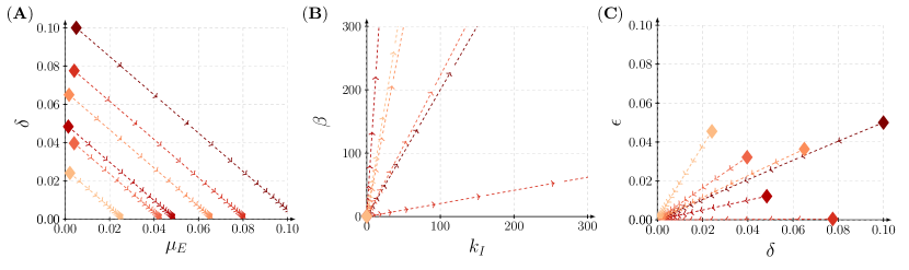
Fig. 1: Two-dimensional projections of the action of a parameter symmetry $\Gamma_{\varepsilon}^{\boldsymbol{\theta}}$ of the SEI model. The action of the symmetry $\Gamma_{\varepsilon}^{\boldsymbol{\theta}}$ generated by solving the system of ODEs in Eqs. (111)-(119) for the coefficients $(\alpha_{1},\alpha_{2})=(2,1)$ on six parameters illustrated by diamonds is visualised in three different two-dimensional subspaces of the nine-dimensional parameter space of the SEI model. These subspaces are (A) $(\mu_{E},\delta)$ for which the invariant $I_{3}=\delta+\mu_{E}$ is preserved, (B) $(k_{I},\beta)$ for which the invariant $I_{4}=\beta/k_{I}$ is preserved and (C) $(\delta,\upsilon)$ for which the invariant $I_{5}=\upsilon/(\delta(1-\upsilon))$ is preserved.

First, we visualise the action of this symmetry on three parameter pairs (Fig. 1). These three parameter pairs are $(\mu_{E},\delta)$ for which the symmetry preserves the invariant $I_{3}$ in Eq. (99), $(k_{I},\beta)$ for which the symmetry preserves the invariant $I_{4}$ in Eq. (101) and $(\delta,\upsilon)$ for which the symmetry preserves the invariant $I_{5}$ in Eq. (103). Similarly, we visualise the action of this symmetry on two parameter triplets (Fig. 2). These triplets are $(\beta,\upsilon,c)$ for which the symmetry preserves the invariant $I_{6}$ in Eq. (106) and $(\beta,\delta,k_{E})$ for which the symmetry preserves the invariant $I_{7}$ in Eq. (109).

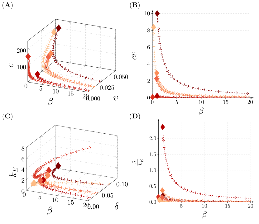
Fig. 2: Three-dimensional projections of the action of a parameter symmetry $\Gamma_{\varepsilon}^{\boldsymbol{\theta}}$ of the SEI model. The action of the symmetry $\Gamma_{\varepsilon}^{\boldsymbol{\theta}}$ generated by solving the system of ODEs in Eqs. (111)-(119) for the coefficients $(\alpha_{1},\alpha_{2})=(2,1)$ on six parameters illustrated by diamonds is visualised in two different three-dimensional subspaces as well as in two different two-dimensional subspaces of the nine-dimensional parameter space of the SEI model. These subspaces are (A) $(\beta,\upsilon,c)$ for which the invariant $I_{6}=\beta c\upsilon$ is preserved, (B) $(\beta,c\upsilon)$ for which the invariant $I_{6}=\beta c\upsilon$ is preserved, (C) $(\beta,\delta,k_{E})$ for which the invariant $I_{7}=\beta\delta/k_{E}$ is preserved and (D) $(\beta,\delta/k_{E})$ for which the invariant $I_{7}=\beta\delta/k_{E}$ is preserved.

4 Discussion

In this work, we have demonstrated how global structural identifiability can be understood in terms of the differential invariants of parameter symmetries. For the last two decades, the notion of classical Lie symmetries of ODEs acting on the independent and dependent variables by mapping solutions to other solutions [12, 13, 14, 15] has been extended to full symmetries which also account for rate parameters. Such full symmetries have been a large focus of research on the structural identifiability of mechanistic ODE models [6, 7, 8, 9, 10], and in particular a large emphasis has been put on developing algorithms for finding such symmetries in an automated fashion. However, the link between algebraic methods for global structural identifiability and symmetry based methods has, until this point, remained elusive. In this work, we established this conceptual link by introducing so-called parameter symmetries, Lie transformations that alter parameters while simultaneously preserving the observed outputs. In addition, we demonstrated that structural identifiability can be understood in terms of the differential invariants of these parameter symmetries. Based on these results, we proposed a three step recipe referred to as the CaLinInv-recipe which involves: (i) re-writing the original first-order ODE system as an equivalent ODE system for the outputs, also referred to as the Canonical coordinates; (ii) finding the parameter symmetries by solving the Linearised symmetry conditions; and (iii) elucidating the global structural identifiability by calculating the differential Invariants of the parameter symmetries. We later validated the CaLinInv-recipe by analysing the structural identifiability of two previously analysed mechanistic models of biological systems.

The CaLinInv-recipe constitutes a new framing of the classical differential algebra approach for elucidating global structural identifiability in terms of Lie symmetries. The steps in this recipe are reminiscent of the differential algebra approach for global structural identifiability (Algorithm 1). In fact, the first steps in the differential algebra approach and the CaLinInv-recipe are identical, and this step attempts at finding algebraic equations relating inputs and outputs with rate parameters [2]. Technically, the differential algebra approach constructs a map between the rate parameters and the parameter combinations that can be inferred from the inputs and outputs, and then structural identifiability implies that this map is injective [21]. The parameter symmetries proposed in this work are essentially such maps, and the injectivity criterion can be understood in terms of the universal differential invariants of parameter symmetries. Better still, by framing global structural identifiability in terms of universal invariants of parameter symmetries, we understand why the standard differential algebra approach, which extracts coefficients in front of the monomials of the polynomial system of output ODEs, always finds identifiable parameter quantities, i.e. universal parameter invariants. This is due to the fact that the coefficients that are extracted in the differential algebra approach will either be a constant or a universal parameter invariant. This property is ensured by the definition of invariants of symmetries combined with the so-called linearised symmetry conditions, the equations defining parameter symmetries. In other words, the standard differential algebra approach is completely consistent with the notion of global structural identifiability expressed in terms of universal parameter invariants. Moreover, our symmetry-based approach for analysing global structural identifiability is theoretically generalisable to other mechanistic models consisting of, say, spatiotemporal systems of partial differential equations but in practice computer-assisted versions of this approach must be developed in order to analyse the global structural identifiability of such systems.

An interesting future research direction is to automate the CaLinInv-recipe for systems of ODEs and eventually systems of partial differential equations. In the context of ODEs, it is known that if the right-hand sides or the reactions terms in the original first-order system are rational functions of the states, it is always possible to re-write the original system of first-order ODEs as a system of ODEs depending solely on the observed outputs [2]. Given such a re-formulated system in terms of the observed outputs, the two remaining steps of the CaLinInv recipe are straightforward to automate using symbolic calculations. This is also why the recipe can be automated, since many existing software for global structural identifiability, e.g. [22], conduct the first step of re-writing the original system so that it solely depends on the observed outputs in an automated fashion. Accordingly, the CaLinInv recipe can be implemented on top of existing algorithms for global structural identifiability analyses based on the differential algebra approach, which would result in an algorithm that not only yields the identifiable parameter combinations but also the family of parameter transformations that preserves the observed outputs, i.e. a family of parameter symmetries.

In total, this work establishes a link between the existing body of work on full symmetries [6, 7, 8, 9, 10] and the differential algebra approach for global structural identifiability [2, 3, 4, 5]. Hitherto, it has been unclear how full symmetries transforming independent and dependent variables as well as parameters relate to global structural identifiability. The result which is closest to such a link was presented by Castro and de Boer [9] which states that a particular parameter is globally structurally identifiable if the only way to scale this parameter by a scaling factor that preserves the observed outputs, is if this scaling factor equals one. In fact, this is exactly what it means to say that the particular parameter of interest is a parameter invariant, and our theoretical framework based on parameter symmetries has formalised this result by demonstrating that a parameter is globally structurally identifiable if and only if it is a universal parameter invariant. Even better, our result generalises to any parameter symmetry as it is not restricted to the scalings studied by Castro and de Boer [9]. A succinct way of expressing our main result is that the globally structurally identifiable parameter quantities are given by universal parameter invariants. We have made a case for a perspective in which global structural identifiability is expressed in terms of differential invariants of parameter symmetries, and this work is a stepping stone towards fully exploiting the power of symmetry methods within the realm of global structural identifiability.

CRediT author statment

• Conceptualization, Methodology, Visualization (made the figures), Writing - Original Draft, Writing - Review & Editing, Formal analysis (derived and proved theorems and conducted calculations), Software (wrote scripts that conducted calculations).

• Conceptualization, Writing - Original Draft, Writing - Review & Editing.

• Conceptualization, Writing - Original Draft, Writing - Review & Editing,

• Conceptualization, Writing - Original Draft, Writing - Review & Editing.

References

• [1] Oana-Teodora Chis, Julio R Banga, and Eva Balsa-Canto. Structural identifiability of systems biology models: a critical comparison of methods. PLOS ONE, 6(11):e27755, 2011.
• [2] Lennart Ljung and Torkel Glad. On global identifiability for arbitrary model parametrizations. Automatica, 30(2):265–276, 1994.
• [3] Hoon Hong, Alexey Ovchinnikov, Gleb Pogudin, and Chee Yap. Global identifiability of differential models. Communications on Pure and Applied Mathematics, 73(9):1831–1879, 2020.
• [4] M Pia Saccomani, Stefania Audoly, Giuseppina Bellu, and Leontina D’Angio. A new differential algebra algorithm to test identifiability of nonlinear systems with given initial conditions. In Proceedings of the 40th IEEE Conference on Decision and Control (Cat. No. 01CH37228), volume 4, pages 3108–3113. IEEE, 2001.
• [5] Eric Walter and Yves Lecourtier. Global approaches to identifiability testing for linear and nonlinear state space models. Mathematics and Computers in Simulation, 24(6):472–482, 1982.
• [6] James W T Yates, Neil D Evans, and Michael J Chappell. Structural identifiability analysis via symmetries of differential equations. Automatica, 45(11):2585–2591, 2009.
• [7] Benjamin Merkt, Jens Timmer, and Daniel Kaschek. Higher-order Lie symmetries in identifiability and predictability analysis of dynamic models. Physical Review E, 92(1):12920, 2015.
• [8] Gemma Massonis and Alejandro F Villaverde. Finding and breaking lie symmetries: implications for structural identifiability and observability in biological modelling. Symmetry, 12(3):469, 2020.
• [9] Mario Castro and Rob J de Boer. Testing structural identifiability by a simple scaling method. PLOS Computational Biology, 16(11):1–15, 2020.
• [10] Alejandro F Villaverde. Symmetries in Dynamic Models of Biological Systems: Mathematical Foundations and Implications. Symmetry, 14(3):467, 2022.
• [11] Alejandro F Villaverde and Gemma Massonis. On testing structural identifiability by a simple scaling method: relying on scaling symmetries can be misleading. PLOS computational biology, 17(10):e1009032, 2021.
• [12] George W. Bluman and Sukeyuki Kumei. Symmetries and differential equations. Springer Science & Business Media, New York, 1989.
• [13] Peter E. Hydon. Symmetry methods for differential equations: a beginner’s guide. Cambridge University Press, New York, 2000.
• [14] Peter J Olver. Applications of Lie groups to differential equations. Springer Science & Business Media, New York, 2000.
• [15] Hans Stephani. Differential equations: their solution using symmetries. Cambridge University Press, New York, 1989.
• [16] Marissa Renardy, Denise Kirschner, and Marisa Eisenberg. Structural identifiability analysis of age-structured PDE epidemic models. Journal of Mathematical Biology, 84(1-2):9, 2022.
• [17] Stefania Audoly, Giuseppina Bellu, Leontina D’Angio, Maria Pia Saccomani, and Claudio Cobelli. Global identifiability of nonlinear models of biological systems. IEEE Transactions on Biomedical Engineering, 48(1):55–65, 2001.
• [18] Victor W Bolie. Coefficients of normal blood glucose regulation. Journal of Applied Physiology, 16(5):783–788, 1961.
• [19] Claudio Cobelli and Joseph J Distefano 3rd. Parameter and structural identifiability concepts and ambiguities: a critical review and analysis. American Journal of Physiology-Regulatory, Integrative and Comparative Physiology, 239(1):R7–R24, 1980.
• [20] Aaron Meurer, Christopher P. Smith, Mateusz Paprocki, Ondřej Čertík, Sergey B. Kirpichev, Matthew Rocklin, AMiT Kumar, Sergiu Ivanov, Jason K. Moore, Sartaj Singh, Thilina Rathnayake, Sean Vig, Brian E. Granger, Richard P. Muller, Francesco Bonazzi, Harsh Gupta, Shivam Vats, Fredrik Johansson, Fabian Pedregosa, Matthew J. Curry, Andy R. Terrel, Štěpán Roučka, Ashutosh Saboo, Isuru Fernando, Sumith Kulal, Robert Cimrman, and Anthony Scopatz. Sympy: symbolic computing in python. PeerJ Computer Science, 3:e103, January 2017.
• [21] Xabier Rey Barreiro and Alejandro F Villaverde. Benchmarking tools for a priori identifiability analysis. Bioinformatics, 39(2):btad065, 2023.
• [22] Ruiwen Dong, Christian Goodbrake, Heather A. Harrington, and Gleb Pogudin. Differential elimination for dynamical models via projections with applications to structural identifiability. SIAM Journal on Applied Algebra and Geometry, 7(1):194–235, 2023.
Acknowledgements
JGB is funded by a grant from the Wenner-Gren foundations (Grant number: FT2023-0005). JBG thanks the Wenner-Gren foundations for a research fellowship. APB thanks the Mathematical Institute, Oxford for a Hooke Research Fellowship. This work was supported by a grant from the Simons Foundation (MP-SIP-00001828, REB)