Theory and simulations of few-photon Fock state pulses strongly interacting with a single qubit in a waveguide: exact population dynamics and time-dependent spectra
Abstract
We present a detailed quantum theory and simulations of a few-photon Fock state pulse interacting with a two-level system (TLS) in a waveguide. For a rectangular pulse shape, we present an exact temporal scattering theory for the waveguide-QED system to derive analytical expressions for the TLS population, for 1-photon and 2-photon pulses, for both chiral and symmetric emitters. We also derive the stationary (long time) and time-dependent spectra for 1 photon excitation, and show how these differ at a fundamental level when connecting to TLS population effects. Numerically, we also present matrix product state (MPS) simulations, which allow us to compute more general photon correlation functions for arbitrary quantum pulses, and we use this approach to also show results for Gaussian quantum pulses, and to confirm the accuracy of our analytical results. In addition, we show how significant population TLS effects also occur for pulses relatively long compared to the radiative decay time (showing that a weak excitation approximation cannot be made), and investigate the population signatures, nonlinear features and dynamical behavior as a function of pulse length. These detailed theoretical results extend and complement our related Letter results [Arranz Regidor et al., unpublished, 2024].
I Introduction
Waveguides can couple to localized quantum emitters in ways that are not possible with cavities, opening up rich light-matter coupling regimes [1, 2, 3, 4, 5, 6, 7, 8, 9, 10]. In a quantum optics picture, such systems facilitate “waveguide-QED,” which can be realized in various material systems, including atoms, molecules, quantum dots, and superconducting qubits, and these schemes use various waveguide environments [11, 12, 13, 14, 15, 16, 17, 18, 19, 20, 21, 22].
With superconducting waveguides (transmission lines, which use microwave photons), qubits can be arranged as “giant-atoms,” where multiple qubits can be collectively coupled with great precision at various spatial points, typically separated in such a way as to cause either destructive or constructive interference [23, 24, 25, 26]. In atomic systems, laser-cooled atoms can also be trapped in nanofibers, evanescently coupled to the propagating fiber modes. From a practical perspective, semiconductor quantum dots (grown within semiconductor waveguides) behave as ideal quantum emitters, emitting optical photons on-chip with very large waveguide beta factors [27, 28, 29] (i.e., almost all of the emitted photons are into the waveguide mode of interest). Such waveguides also offer rich design flexibility, and, for example, one can easily tune the chirality of the emitter coupling [30, 31], opening up other areas of study such as chiral networks [32, 33, 34, 35, 36, 37].
From a theoretical perspective, various approaches have been used to describe waveguide-QED systems, often with various levels of approximation. For example, with a weak excitation approximation (WEA), usually the problem can be solved within the domain of linear response, for example, using Green function techniques, allowing easy access to the polariton states, even for collective multi-emitter systems [38]. However, such approximations cannot be done in the ultrastrong coupling regime [39, 40], where unique quantum waveguide-QED effects appear from not making a rotating wave approximation[41, 42, 43, 44]. For the regimes of interest in this paper, we will safely assume the rotating wave approximation (since we are interested in a single emitter whose waveguide couping rate is much smaller than the transition frequency).
At the quantum field level, other simplified approaches also exist, for example, instantaneous master equations, and 2nd-order Born-Markov solutions where the waveguide can be traced out [45, 14]. Unfortunately, such approaches are not suited to look at some of the unique quantum light-matter entanglement that can occur when one treats the waveguide photons exactly, in a regime where the photons and emitters interact strongly.
One of the simplest waveguide-QED systems is a single qubit coupled to a waveguide, which already admits various non-trivial solutions. Fan and coworkers have developed powerful scattering theories to model such systems, usually specialized to model the long-time output states with respect to the input states, allowing for a powerful description of the transmitted and reflected quantum fields, while fully accounting for the TLS [46, 47, 48, 49]. In a waveguide-QED single TLS system, when the waveguide mode interacts strongly with the TLS, the often used WEA can drastically fail, even when one uses temporally short quantum fields at the level of one photon (a single Fock state). Indeed, it has been shown that one can fully invert a TLS when the appropriate temporal excitation is employed [50]. Despite this, the WEA is still commonly employed in many scattering theories, and it is not generally well known when such an approximation works in terms of the excitation fields. It is also not well appreciated if the single excitation, which can still yield significant population transfer and photon-matter entanglement, shows any spectral signatures, as one still expects a linear response from a single photon excitation, which is usually well described at the level of a simple classical harmonic oscillator.
More direct time-dependent modelling of few photon scattering can be modelled by solving the time-dependent Schrödinger equation [51, 52], or solving the relevant Heisenberg equations of motion [53, 54]. For easier access to the multi-photons, time retardation effects and various causality-modified correlation effects, matrix product states (MPS) is a powerful tensor network approach to solve the entire waveguide-QED system in a numerically exact way [55, 56, 57, 58, 59, 60, 37], in principle only limited by numerical step sizes, etc, which can easily be checked for good numerical convergence.
In this work, we complement our related Letter paper [61], by presenting a detailed theoretical study of how a few-photon pulse interacts with a single TLS in a waveguide. We first present a real-space time-dependent solution to obtain analytical results for both 1-photon and 2-photon (Fock state) pulses, for the TLS population. We also describe our MPS approach, and use both these methods to connect to the stationary as well as the time-dependent spectra, presenting a selection of results for both a symmetric TLS and a chiral TLS.
One of our interesting findings is that the population dynamics of a 1-photon-pulse excitation completely cancels out in the transmitted spectra, but it remains an observable for the time-dependent spectra, which directly relates to similar observables that were measured recently with classical pulses in the regime of semiconductor quantum dot cavity systems [62, 63]. We also show how the 2-photon results yield significantly different stationary spectra, as well as dynamic (time-dependent) spectra. Finally, we study how the peak TLS populations depend on the pulse duration, and present solutions for both top-hat pulse shapes as well as Gaussian pulses.
The rest of our article is arranged as follows. First, in Sec. II, we derive an analytical solution for the TLS population using a rectangular (top-hat) temporal quantum pulse containing one photon, for both chiral and symmetrical quantum emitters. We then extend this approach in Sec. III to a 2-photon quantum pulse with the same temporal shape.
In Sec. IV, we derive an analytical solution for the stationary spectrum (i.e., the long time limit) with a one-photon excitation pulse, again for both the symmetrical and chiral emitter case. Here, we see how all the TLS population effects that we observed in the previous sections cancel out, and in the chiral case we simply recover a spectrum that is identical to the input pulse. In order to further investigate this effect and go beyond the long time limit result, in Sec. V, we derive an analytical solution for the chiral time-dependent spectrum. We start by deriving the transmitted mean photon population in Sec. V.1. Then, in Sec. V.2, we derive the transmitted first-order photon correlation functions, knowing that in the limit when , these simply recover the mean photon population previously calculated. Here, we also verify our results by calculating the same observable using MPS, and show excellent agreement. Next, Sec. V.3 shows the relation between the first-order photon correlations, and the time-dependent spectrum and spectral intensity.
In Sec. VI, we introduce the MPS theoretical approach we use that can be used to calculate 1-photon and 2-photon quantum pulses with any given temporal shape.
Population results (for the TLS and transmitted fields) are shown in Sec. VII, where we start by calculating the populations of a symmetrical TLS emitter and compare them with the chiral results shown in Ref. [61] (Sec. VII.1); we then study the influence of pulse duration on the TLS populations in Sec. VII.2, where we observe that populations are considerable even for relatively long pulses, still showing results that clearly deviate from any WEA results. Indeed, we observe that we do not recover the WEA results until the pulse durations are on the order of , where is the total TLS decay rate into the waveguide.
In Sec. VIII, we show example analytical results for the time-dependent spectra and spectral intensity for a 1-photon rectangular quantum pulse with a chiral emitter, and confirm that the results agree with the calculations performed using MPS, shown in Ref. [61]. In addition, we use MPS to show the symmetrical TLS case with rectangular pulses containing 1 and 2 photons. For chiral TLSs, we also show the time-dependent spectra for 1-photon and 2-photon pulses, for several longer pulse durations ( and ), demonstrating pulse break up effects for intermediate pulse lengths ().
II Analytical Solutions for the Two-Level-System Population with a One-Photon (Fock State) Pulse
We consider an infinite waveguide, that supports a target forward and backward waveguide mode below the light line, and is thus lossless. This could be in the form of a semiconductor nanowire, a circuit-QED waveguide, or a photonic crystal waveguide—which allows lots of flexibility in how one couples to artificial atoms such as quantum dots [16, 32, 64, 65, 11, 66, 67, 68].
Since we are dealing with forward (e.g., to the right) and backward (to the left) propagating modes for waveguides, we can derive space-time solutions for the (quasi) one-dimensional (1D) envelopes of the waveguide mode operators, which satisfy the following propagation equation:
| (1) |
where and label ‘right’ and ‘left’ propagating fields, and we have expanded the waveguide dispersion solution as () or (), i.e., we assume linear dispersion at some frequency of interest, , which is below the light line. The mode is assumed to be lossless.
Defining , we can also write in the rotating frame,
| (2) |
which are the 1D envelopes for the slowly-varying waveguide mode operators. The boson operators satisfy the fundamental commutation relations,
| (3) |
where and have units of . These operators describe the creation of a right- and left-moving state at position , respectively, and allow us to introduce a real space picture for the Hamiltonian description below.
For the TLS-waveguide system, we start with the following total Hamiltonian,
| (4) |
where the free (uncoupled) waveguide term is
| (5) |
and the free TLS term, in the Heisenberg picture (where operators are time-dependent in general), is
| (6) |
where is the detuning between the TLS, with a resonant frequency , and the waveguide mode pulse, with the main frequency ; thus, for on resonance, .
For the TLS-field interaction term, after using a dipole and rotating wave approximation, we have
| (7) |
which, for a single TLS at , yields
| (8) |
where we introduced the photon-TLS coupling term (with right and left coupling indices), for an atom at position . This waveguide photon-TLS coupling term is defined from
| (9) | |||
| (10) |
where is an effective mode volume (per unit cell), is the dipole moment, and has units of inverse volume, with the normalization [27]. Note that we write for brevity, and these coupling strengths have units of . Here is the pitch in the case of a photonic crystal waveguide, or a length associated with periodic boundary conditions. We can also relate this to the TLS population decay rate, , so that
| (11) |
in agreement with known results for photonic crystal waveguides [27, 31].
The transmitted and reflected fields can be calculated from the corresponding equations of motion for the photon operators,
| (12) |
Using the result of the unperturbed field from Eq. (2), together with Eq. (8) and Eq. (3), we obtain
| (13) |
and after integrating,
| (14) |
Note that the input fields contain noise fields (or free fields) as well as any considered quantum source.
Now, considering a right input field operator, and neglecting vacuum noise terms as they will not contribute in normal ordering), and , then the transmitted field is
| (15) |
while the reflected field (to the left of the TLS) is
| (16) |
It is important to note again that has units of and, consequently, has the same units.
Let us now assume , with a right (forward) propagating input field, and using , then
| (17) |
and
| (18) |
For any temporal input pulse shape (which modulates the input quantum state), normalized with
| (19) |
we can define the input operator as , with . The temporal pulse has a center frequency , and propagates freely in the waveguide in the absence of a TLS. The pulse bandwidth is then determined by the quantum pulse time duration and temporal profile.
For a 1-photon pulse, we need to satisfy
| (20) |
which enables us to obtain for a 1-photon input state. Note also that
| (21) |
Thus, to obtain a normalized pulse containing one photon, , and the input boson operator is
| (22) |
which depends also the normalized pulse shape , and the annihilation operator , which annihilates a photon in the waveguide, with the relation: .
II.1 Symmetrical Emitter (Two-Level System) Solution
To obtain the expectation value of the TLS population, we seek to solve the appropriate differential equations of motion in the Heisenberg representation. We first consider the case of symmetrical TLS coupling. The equation of motion for is obtained from:
| (23) |
with and , with real, Equation (23) gives
| (24) |
Next, we derive the differential equation for the TLS population,
| (25) |
which shows explicitly the radiative emission rate, , in the absence of any quantum input pulse.
Now, if we apply the differential equation to an input pulse containing one photon, we obtain
| (26) |
and
| (27) |
Considering the resonant case, i.e., , then we have
| (28) |
This general approach can be extended to pulses with a higher number of photons () [54],
| (29) |
where represents the photon number and is the pulse shape. To solve Eq. (29), we also need the more general coherence equation of motion
| (30) |
For the case of a rectangular pulse, of length , containing one photon, the pulse envelope is defined from
| (31) |
and Eq. (29) transforms to
| (32) |
II.2 Chiral Emitter Solution
In the case of having a chiral TLS system, where and (which is the one studied in Ref. [61], our companion Letter), the relevant interaction equations of motion are now
| (38) |
and
| (39) |
Considering again the system on resonance, then
| (40) |
Now using this with the one-photon rectangular pulse, and considering that in the chiral case, , (for , i.e., while the pulse is being applied), we obtain
| (41) |
Integrating this equation gives
| (42) |
and the time-derivative for the population is derived to be
| (43) |
and thus
| (44) |
Subsequently, the relevant differential equations of motion in this case are as follows:
| (45) | |||
| (46) |
III Analytical Solution for the Two-Level-System Population using a Two-Photon Pulse
III.1 Symmetrical Emitter Population Dynamics
Using the same top-hat pulse profile as before, we now consider a 2-photon excitation pulse. While , Eqs. (29) and (30) transform to
| (48) |
and
| (49) |
where the last term contains the 1-photon solution, derived explicitly in the previous subsection. Using Eq. (47), then
| (50) |
and after integrating Eq. (50), we obtain
| (51) |
We can use this result to solve Eq. (48), so that:
| (52) |
and then the TLS population, while , is
| (53) |
III.2 Chiral Emitter Population Dynamics
The population equation of motion in a chiral emitter system transforms to
| (57) |
Using the chiral solution for the 1-photon pulse, Eq. (49) gives
| (58) |
Integrating this, using in Eq. (57) and proceeding in the same manner as in the symmetrical case, we obtain the 2-photon TLS population solution for the chiral system,
| (59) |
IV Analytical Solution for the One-Photon Stationary Spectra
IV.1 One-photon stationary spectra for the symmetrical emitter
We next calculate the transmitted stationary (long time) spectrum, , from
| (60) |
The first term of Eq. (60) is
| (61) |
which is just the spectrum of the incidence pulse. For the symmetrical coupling case, where , the second term is
| (62) |
In order to solve , we need to use the equation of motion for [Eq. (24)], and perform a Fourier transform to obtain:
| (63) |
and thus
| (64) |
Applying this to Eq. (62), gives
| (65) |
To calculate the right hand side, we use
| (66) |
Inserting this result in Eq (65), gives
| (67) |
Finally, the last term of Eq. (60) can be solved using the previous results, and we obtain
| (69) |
Adding up all the previous terms, we obtain
| (70) |
where the second term represents a drop on the transmitted spectrum due to reflection from the TLS.
This is exactly the same result as a bosonic emitter, namely a harmonic oscillator model for the atom or qubit, which also coincides with the result from a WEA, for this function. However, clearly the terminology of a “weak excitation” is not appropriate here, as the atom can indeed be efficiently excited; it just happens to yield the same stationary spectrum result as a bosonic atom in the strict one quantum subspace. Indeed, we could also simply have replaced much earlier in the derivation, and identical final results will be obtained for the 1-photon case, but such an approximation would get the wrong dynamical result, discussed in more detail later.
Note to obtain Eq. (70), we have exploited the convolution theorem: , and . In this case, and , and
| (71) |
IV.2 One-photon stationary spectra for the chiral emitter
As before, we can calculate the stationary spectrum, , from Eq. (60), where the first term is again
| (72) |
and the equation of motion for is
| (73) |
If we perform a Fourier transform to Eq. (73),
| (74) |
then
| (75) |
and
| (76) |
The third term takes the form,
| (77) |
and the last term is
| (78) |
Adding up all the previous terms, we simply get the trivial result
| (79) |
and the transmitted spectrum is identical to the input spectrum in this chiral case where the emitter radiates only to the right (at least for the stationary spectrum case).
It is important to stress that the cancellation of the final three terms only occurs for the time-integrated spectra as we show below, since the population dynamics of the TLS indeed affect the time-dependent spectra, even for a 1-photon pulse. The chiral emitter results are shown in Ref. [61], where the long-time limit spectra for 1-photon pulses are calculated for different pulse lengths, and in all cases they show agreement with Eq. (79).
V Solution for the chiral time-dependent spectrum
Here we will first derive the population terms and then the time-dependent spectrum for the field after interacting with the quantum chiral emitter. Results for a non-chiral emitter can be derived in a similar way.
V.1 Derivation of the transmitted photon mean population
In general, the transmitted and reflected flux can be calculated from
| (80) |
where and , as before, refer to the right (transmitted) and left (reflected) photons, respectively.
We start by deriving the chiral solution for the time-dependent transmitted photon flux, which is needed for the initial condition of the two-time correlation functions,
| (81) |
The first term of Eq. (81) is
| (82) |
while the second term is
| (83) |
The coherence term evolves as
| (84) |
and after integrating,
| (85) |
Introducing this in Eq. (83), gives
| (86) |
While for the third term, we obtain
| (87) |
Finally, to calculate the last term in Eq. (81), we can use Eq. (26), and considering the chiral case, then
| (88) |
Assuming the resonant case (), then
| (89) |
To further check that this general solution is correct, we can calculate the TLS population for a rectangular pulse (since we worked this out earlier),
| (90) |
and after integrating,
| (91) |
which perfectly agrees with the result calculated in Eq. (46).
The more general integrated expression (in the resonant chiral case), for arbitrary pulse shapes, is
| (92) |
Finally putting everything together, we obtain the transmitted photon population:
| (93) |
We observe here that, in general, the TLS interaction terms do not cancel out, even for the non-resonant case (). Thus (apart from the case of relatively very long pulses, quantified later) a WEA would not make sense here, and produce the wrong result, even if it happens to yield the same stationary spectrum.
The transmitted flux for the rectangular pulse can be calculated by considering the four terms in Eq. (81). For the first term in this case,
| (94) |
while for second term,
| (95) |
For the third term,
| (96) |
and for the last term, we can use the solution of the TLS population, so that
| (97) |
Putting everything together, we obtain the desired solution for the transmitted photon flux for a chiral TLS interaction:
| (98) |
We note that for , the only term contributing is the TLS population one. The symmetric system can be derived in a similar way, which yields both transmitted and reflected fields.
V.2 Derivation of the transmitted first-order photon correlation function
Considering the same chiral system as above, we now wish to calculate , since this is needed to connect to the time-dependent spectra. This two-time correlation function is obtained from
| (99) |
which we have split into four parts for analysis purposes.
To solve these, we can first use Eq. (41) for any general pulse shape:
| (102) |
which gives a formal solution,
| (103) |
Introducing this in Eq. (101), gives
| (104) |
which will depend on the pulse profile, , used in each case.
The third term in Eq. (99) can be derived in a similar way,
| (105) |
Finally, to calculate the last term of Eq. (99), we need to use the quantum regression theorem,
| (106) |
where one uses as the initial condition, so clearly the time-dependent TLS population plays a significant role here.
For a rectangular pulse, the previous terms can be derived analytically,
| (107) |
The second term, in this case, gives
| (108) |
The third term becomes
| (109) |
Finally, the fourth term is,
| (110) |
We highlight that this last term is the only term contributing to the correlation function when , showing a clear influence from the TLS population effects. We have also confirmed that the above analytical expressions agree perfectly with those obtained numerically using MPS (Sec. VI), as shown in Fig. 1.
V.3 Time dependent spectra and spectral intensity
In a rotating wave approximation, the time-dependent spectrum is obtained from the two-time first-order correlation functions calculated in Sec. V.2, using
| (111) |
where .
The time-dependent spectral intensity can also be calculated from the same two-time correlation functions:
| (112) |
Here, it is important to note that the integration of Eq. (112) over time, , agrees with the stationary spectra, i.e., [62], so the time-integrated spectral intensity is equivalent to the long-time spectra, even though and contain very different dynamical signatures.
VI Matrix Product States approach
In order to extend the analytical results previously calculated, we have also made use of MPS, which is an exact numerical approach based on tensor network theories [59, 60].
Using the MPS approach, the system, which contains both the TLS and the waveguide, is discretized in time. The state is decomposed in a tensor product by performing Schmidt decompositions (or singular value decompositions). Each of the tensors receives the name of ‘bin’, with the TLS as the ‘TLS bin’ and the photonic part as the ‘time bins’ [69, 70].
The quantum pulse is contained in the photonic part of the initial state [56]. If we have an initial state,
| (113) |
where corresponds to the TLS part and to the photonic part, where each time bin contains a tensor product of the right and left channels at the corresponding time step. Thus, a 1-photon pulse will be introduced from
| (114) |
where
| (115) |
where is normalized as before, and
| (116) |
is the quantum noise creation operator in the time domain with the commutation relations where correspond to the left and right channel, respectively [53]. In this case, for a right propagating pulse, the input pulse is introduced in the right channel,
| (117) |
Writing this in the MPS description,
| (118) |
where is the discretized version of which contains the shape of the pulse at each time bin,
| (119) |
is the quantum noise creation matrix product operator (MPO), with the commutator , and is a time step. It is important to note that has units of , hence, to calculate the photon flux as in Eq. (80) with the MPS approach,
| (120) |
Considering this, can be written as follows:
-
•
if :
(121) -
•
if :
(122) -
•
if :
(123)
where, in this case, each has 2 dimensions corresponding to 0 and 1 excitations.
For a 2-photon pulse, we have
| (124) |
and the tensors now contain another dimension to count for the two excitations:
-
•
if :
(125) -
•
if :
(126) -
•
if :
(127)
This is then transformed to have the required canonical shape, where we have the Orthogonality Center (OC) in the present time bin and the rest of the pulse time bins are left normalized, in order to combine them with the TLS bin, and solve the time dynamics as usual. This method can be easily extended to pulses containing higher numbers of photons.
VII Photon Population and Two-Level-System Population Results
VII.1 Symmetrical emitter
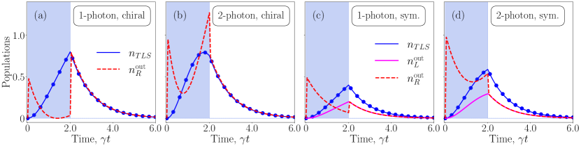
In our related Letter, Ref. 61, we showed specific results for the chiral TLS. For completeness, here we also show them along with the results for the symmetric TLS in Fig. 2. For these simulations, we consider an incident pulse with a width , containing either 1 photon [Figs. 2(a,c)] or 2 photons [Figs. 2(b,d)], which interacts with a chiral TLS with , in Figs. 2 (a,b), and with a symmetrical TLS with in Figs. 2 (c,d).
The observables are calculated using MPS (solid lines), and the TLS population is compared with the analytical solution (blue circles) derived in Sec. II and III, which agree perfectly.
First, in the 1-photon solution, it can be seen that the TLS population of the symmetrical emitter is exactly half the population observed with a chiral TLS. This agrees with the analytical results from the previous sections. However, the 2-photon solution deviates from this, due to the photon non-linear interactions. Additionally, the transmitted and reflected flux are shown in dashed red and solid magenta, respectively, where the nonlinearities of the 2-photon can again be observed.
The photon flux from Eq. (80) can be integrated in time, yielding
| (128) |
When this quantity is added to the TLS population, we recover the number of quantum excitations in the system. For example, for a chiral emitter, this is
| (129) |
and for a symmetrical case we now need to consider both the transmitted and reflected flux, so that
| (130) |
where
is the instantaneous TLS population.
In both cases, for a 1-photon pulse, and
for the 2-photon one.
VII.2 Influence of pulse duration
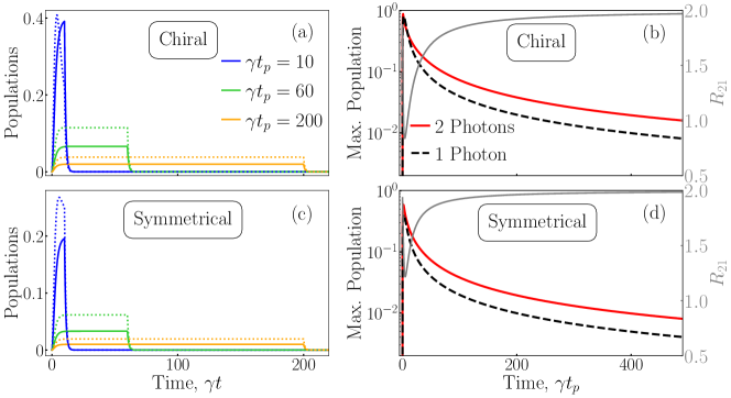
To better understand the time dynamics as a function of pulse duration, in Fig 3 we study the TLS population for different pulse lengths for 1- and 2- photon pulses.
In Figs 3(a,c), the TLS populations are shown for 1-photon pulses (solid lines) and 2-photon pulses (dotted lines) with three different pulse lengths: (blue), (green) and (orange). Figure 3(a) shows the chiral solution while Fig. 3(c) is the symmetrical solution. We observe a clear deviation from the WEA approximation in every solution with significant population dynamics in all the results. Indeed, the excitation of the TLS is still considerable even for pulses as long as . In addition, we see how the population nonlinearites between the 1-photon and 2-photon solutions appear more in the shorter pulses, where they both have highly different dynamics, but when the pulses get long enough, they reach a plateau, and the two-photon solution tends to just double the single photon one.
In order to see the trend of population ratios more clearly, in Figs. 3(b,d), the maximum values of the TLS population are shown versus the pulse duration for the 1-photon pulses (solid red lines) and 2-photon pulses (dashed black lines), where again Fig. 3(b) is the chiral solution and Fig. 3(d) is the symmetrical one. Additionally, the ratio between both solutions are computed from:
| (131) |
Here, we highlight two important effects: (i) it can be seen that the TLS population does not tend to zero until remarkably long pulses () even in the 1-photon solution, showing that the WEA does not hold for these longer pulses; and (ii), the ratio between the maximum population for the 2-photon solution and the 1-photon only tends to two only for sufficiently long pulses, which indicates that there are nonlinearities in the 2-photon solution even for these relatively long pulses. This is important as often a WEA is assumed in models of quantum pulses interacting with TLSs in waveguides, and our theory allows one to quantify if this is valid or not.
VIII Stationary and Time-Dependent Spectral Results
For the limit of 1-photon excitation, we found the interesting result that the time-dependent spectrum evolves to exactly the same spectrum as the input pulse when working with a chiral system. To better understand this, consider the earlier derived long-time spectrum, , for a chiral pulse [Eq. (79)],
| (132) |
which is a consequence of the fact that the population and TLS effects completely cancel out.
Clearly, this is different in the time-dependent case [], when time is not in the long time limit. For instance, if we study the in the region where , the only term remaining is fourth term of Eq. (99), , therefore dominating the dynamics in this region,
| (133) |
which requires as the initial condition,
| (134) |
Equation (134) resembles closely Eq. (47), i.e. the population dynamics, showing that TLS population effects directly affect both and .
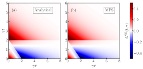
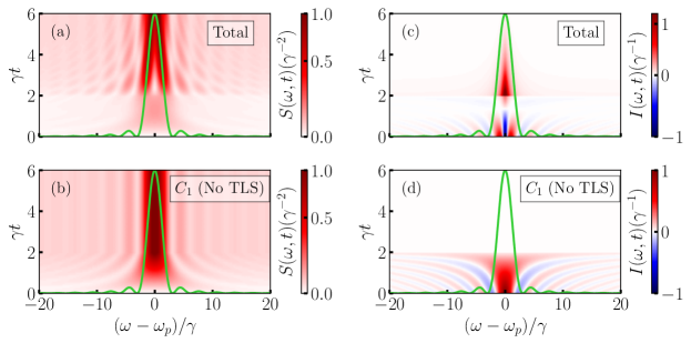
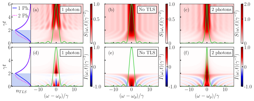
Figure 5 shows the analytical solution of the time-dependent spectrum, , of a 1-photon rectangular quantum pulse with interacting with a chiral TLS. In Fig. 5(a) we can see the full solution and in Fig. 5(b), the solution when we do not consider population effects (only considering the first term of the first order correlation function, ). First of all, we can see again the agreement between the analytical results and the ones calculated using MPS (see Ref. [61]). In addition, these results show the importance of considering the population dynamics when calculating the time-dependent spectrum. The solution with only the first term of the analytical solution, , gives the same results as when not considering the TLS when solving the problem.
This is additionally shown in Fig. 5(c,d) where the spectral intensity is calculated for the same cases. Again, from this result, we can clearly see the contribution of the population dynamics.
Note that unphysical solutions are obtained if we simply neglect the population term () in computing the spectra, where the sum of yield negative spectra with qualitatively different features.
These analytical results agree agree perfectly with the numerical results shown in Ref. 61, which are reproduced in Fig. 5, where we also show the 2-photon spectra (in part to compare with the symmetric TLS results discussed next).
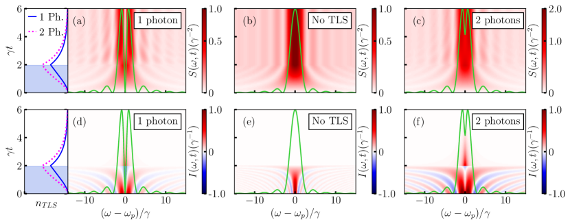
Clearly, this population behavior is not exclusive to the chiral solution, and in Fig. 6, we show the time-dependent spectral results when considering a symmetrical emitter. The spectrum and the spectral intensity are calculated using MPS, where we use again a rectangular pulse of pulse length containing one photon Fig. 6(a,d). For comparison, the same observables are calculated without TLS interaction in Fig. 6(b,e). We observe how, in the stationary spectra, where we recover the harmonic oscillator solution. However, the population effects are evident in both the dynamical spectrum and the spectral intensity, with results that highly differ from the case with no TLS. For instance, in the spectral intensity [Fig. 6(d)], we observe positive values at times longer than the pulse length (for ), while these effects are (obviously) not visible when there is not a TLS interacting with the pulse [Fig. 6(e)].
Further, we have also calculated the solution for a 2-photon pulse with the same pulse length () interacting with the symmetrical emitter [Fig. 6(c,f)], where we again observe similar population effects. However, in this case we can also observe the population effects in the stationary spectrum (represented by the green solid line).
Influence of pulse duration on the transmitted spectra
As previously seen in Sec. VII.2, the TLS population dynamics depend on the pulse duration, with results that deviate from the WEA approximation and visible nonlinear effects in the case of 2-photon pulse.
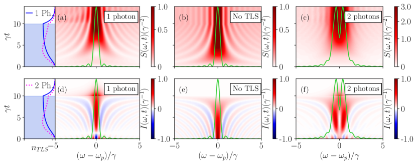
We next examine the role of using a longer pulse on the emitted spectra. In Fig. 7, the spectra and spectral intensity are calculated for a chiral TLS interacting with a rectangular pulse of length , containing 1 photon Fig. 7 (a,d) and 2 photons Fig. 7 (c,f). The pulse results with no interaction are shown in Fig. 7(b,e). Here, we observe how the TLS effects can still be appreciated in both cases, with solutions that deviate from the cases with no TLS interaction. In the 1-photon solutions, we observe how the presence of the TLS effects start to become more subtle. However, in the 2-photon cases, the nonlinearities are still very present, where we can even see a stronger break up of the pulse in frequency. Similar pulse break up effects have been found in [37] using ensembles of chiral emitters.
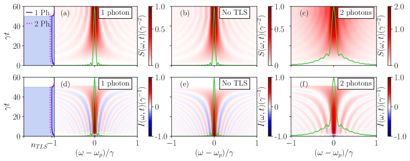
In Fig. 8, we show results similar to the previous ones, but with an even longer pulse (). In this case, we observe solutions that are much closer to the case with no TLS. Specifically, in the one-photon solutions, some small dynamical effects can still be seen when the pulse turns on and off, with the populations reaching a quasi- steady-state during most of the pulse. The two-photon solution still has some significant deviations from the case without the TLS interaction, but shows no visible pulse break up effects (caused by TLS saturation).
These results confirm that the dynamical effects seen in the spectral results are directly related to the TLS population effects and that they persist as long as there is a reasonable TLS population.
IX Gaussian pulses
For completeness, we next show results for few-photon excitation with Gaussian pulses, since the MPS results can use arbitrary waveforms. In this case, the temporal pulse has the following normalized shape,
| (135) |
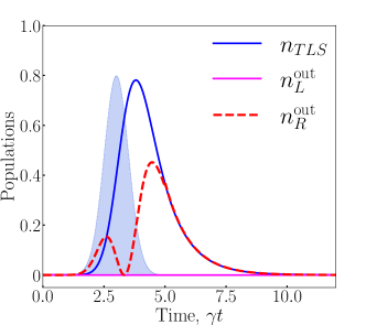
where is the center of the pulse and is its width. Figure 9 shows the various populations, for a 1-photon pulse, with a width of and centered at , interacting with a chiral emitter. Here again, the shaded blue area represents the incident pulse, the solid blue line is the TLS population, and the red dashed line represents the normalized transmitted photon population. Interestingly, there is an instant that the photon population is zero in this case (just after the center of the pulse). Additionally, the left photon population stay at zero at all times since this is a chiral system.
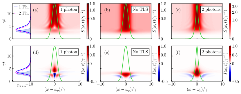
The corresponding spectral functions and are shown in Fig. 10. To better appreciate the influence of population effects on the dynamical spectrum, in Fig. 10, again we show both the population decay and the dynamic spectra side by side. As also seen in Fig. 9, one can clearly observe in Fig. 10(a) the effects of the TLS population dynamics, which causes a spectral hole and additional interferences. This can be appreciated by comparing these solutions with the corresponding without the TLS, shown in Fig. 10(b). However, as in the case of the rectangular pulse, in the long time limit, all the population effects get cancelled and we recover the same stationary spectra in both cases (green solid lines).
In addition, rich features are observed in the spectral intensity in Fig. 10(d), where again, by comparison with the case without the TLS [Fig. 10(e)], we see additional interferences during the pulse, and intensity positive values after the pulse while the TLS is decaying, that cannot be observed without this interaction. Nevertheless, if we integrate the spectral intensity in both cases, we again recover the same solution which agrees with the stationary spectra (green solid lines).
Finally, Figs. 10(c) and (f) show the same spectral observables, and respectively, when using a similar Gaussian pulse but now containing 2 photons. Here we see again the TLS dynamical effects in both cases, and, in agreement with what we saw with rectangular pulses, the stationary spectrum now shows the nonlinear excitation, with a narrower width and a more pronounced central peak.
These results show further details about how population dynamics influence the spectral plots, and also which ones are due to the specific shape of the pulse used as well (e.g., showing convolution effects with a sinc function or a Gaussian function). Note also, that an analytical solution for the 1-photon excitation is possible in terms of the error function (or via a numerical integration), but may not be so easy to obtain for the two-photon case.
X Conclusions
We have presented a detailed theoretical analysis of few-photon quantum pulses interacting with a single TLS in a waveguide, using both chiral and symmetric TLS emitters. This complements and adds substantial details and extensions to the results shown in our related Letter [61].
For the theory, we have shown two approaches to compute the TLS population information, visible both in the time dynamics and in certain spectral observables. We started by deriving the analytical solution of the TLS population by solving the corresponding equations of motion in the Heisenberg picture. We have presented the general differential equations for a pulse containing 1 photon, and then solved for a rectangular pulse. Here, we have also shown both solutions with a symmetrical emitter or a chiral emitter that couples only to the right photon channel, and then we have repeated the same procedure for a rectangular pulse containing 2 photons.
Next, we have used the same method to derive the analytical solution for the 1-photon stationary spectra (i.e., in the long time limit). Here, we have seen how all the population effects that were observed in the time dynamics perfectly cancel out, and we recover the same solution with or without the interaction with the TLS (for this observable), for a chiral emitter. For a symmetric emitter, we obtain the same result as a WEA, essentially recovering elastic scattering theory.
In order to better understand these effects, we then introduced a derivation for a time-dependent spectrum, starting with the derivation of the transmitted photon population, and then the transmitted first-order photon correlation functions, and we have shown how these relate to the time-dependent spectra and spectral intensity.
Our analytical results are benchmarked, checked, and extended by using a second theoretical method, based on matrix product states (MPS), which we have introduced after the analytical derivations. This is a tensor network approach which both helped us to verify the analytical solutions, and extend our simulations to more efficient calculations with pulses of different shapes and containing more photons.
After presenting our models, solutions with a rectangular incident pulse are shown, starting with the population results, where a comparison between symmetrical and chiral emitters is shown, for both 1 and 2-photon pulses. In the general cases of short pulses, we have observed high values of TLS populations making clear a deviation from the weak excitation limit. Furthermore, this has been extended with a study of the maximum TLS population as a function of pulse length, and we have seen how the weak excitation approximation is not valid until very long pulses, on the order of . We have also observed in these cases how nonlinear effects are visible in the 2-photon cases until similar lengths. In addition, we showed how the time-dependent spectral profiles depend on the length of the pulse, where eventually the population effects visible for 1-photon pulses become less and less important, and we showed the clear difference between 1-photon and 2-photon pulses.
The spectral results have shown us how population effects influence both the dynamical spectra and the spectral intensity, even though they completely cancel out in the 1-photon stationary solutions. We have also seen that this is not the case when considering a 2-photon pulse, where the nonlinear effects are also seen in the stationary limit, yielding a narrowing of the central pulse peak for a chiral TLS and pulse break up for a symmetric TLS.
Finally, we have calculated similar observables for a Gaussian incident pulse, both containing 1 and 2 photons, interacting with a chiral TLS. In all the cases we observe similar behaviors as in the case of the rectangular pulse (which permits simpler analytical solutions). These results confirm that the findings in this paper are not particular to the shape of the pulse, and can be extended to other pulse shapes as well.
Acknowledgements.
This work was supported by the Natural Sciences and Engineering Research Council of Canada (NSERC) [Discovery and Quantum Alliance Grants], the National Research Council of Canada (NRC), the Canadian Foundation for Innovation (CFI), Queen’s University, Canada, and the Alexander von Humboldt Foundation through a Humboldt Award. We also thank Kisa Barkemeyer, Jacob Ewaniuk, and Nir Rotenberg for valuable contributions and discussions.References
- Sheremet et al. [2023] A. S. Sheremet, M. I. Petrov, I. V. Iorsh, A. V. Poshakinskiy, and A. N. Poddubny, Waveguide quantum electrodynamics: Collective radiance and photon-photon correlations, Rev. Mod. Phys. 95, 015002 (2023).
- Zheng et al. [2010] H. Zheng, D. J. Gauthier, and H. U. Baranger, Waveguide QED: Many-body bound-state effects in coherent and Fock-state scattering from a two-level system, Phys. Rev. A 82, 063816 (2010).
- Witthaut and Sørensen [2010] D. Witthaut and A. S. Sørensen, Photon scattering by a three-level emitter in a one-dimensional waveguide, New Journal of Physics 12, 043052 (2010).
- Roy [2011] D. Roy, Two-photon scattering by a driven three-level emitter in a one-dimensional waveguide and electromagnetically induced transparency, Phys. Rev. Lett. 106, 053601 (2011).
- Crowder et al. [2020] G. Crowder, J. H. Carmichael, and S. Hughes, Quantum trajectory theory of few-photon cavity-QED systems with a time-delayed coherent feedback, Phys. Rev. A 101, 023807 (2020).
- Crowder et al. [2022] G. Crowder, L. Ramunno, and S. Hughes, Quantum trajectory theory and simulations of nonlinear spectra and multiphoton effects in waveguide-QED systems with a time-delayed coherent feedback, Phys. Rev. A 106, 013714 (2022).
- Shen and Fan [2005] J. T. Shen and S. Fan, Coherent photon transport from spontaneous emission in one-dimensional waveguides, Opt. Lett. 30, 2001 (2005).
- Le Jeannic et al. [2022] H. Le Jeannic, A. Tiranov, J. Carolan, T. Ramos, Y. Wang, M. H. Appel, S. Scholz, A. D. Wieck, A. Ludwig, N. Rotenberg, L. Midolo, J. J. García-Ripoll, A. S. Sørensen, and P. Lodahl, Dynamical photon–photon interaction mediated by a quantum emitter, Nature Physics 18, 1191–1195 (2022).
- Longo et al. [2011] P. Longo, P. Schmitteckert, and K. Busch, Few-photon transport in low-dimensional systems, Phys. Rev. A 83, 063828 (2011).
- Crowder et al. [2024] G. Crowder, L. Ramunno, and S. Hughes, Improving on-demand single-photon-source coherence and indistinguishability through a time-delayed coherent feedback, Phys. Rev. A 110, L031703 (2024).
- Türschmann et al. [2019] P. Türschmann, H. L. Jeannic, S. F. Simonsen, H. R. Haakh, S. Götzinger, V. Sandoghdar, P. Lodahl, and N. Rotenberg, Coherent nonlinear optics of quantum emitters in nanophotonic waveguides, Nanophotonics 8, 1641 (2019).
- Pregnolato et al. [2020] T. Pregnolato, X.-L. Chu, T. Schröder, R. Schott, A. D. Wieck, A. Ludwig, P. Lodahl, and N. Rotenberg, Deterministic positioning of nanophotonic waveguides around single self-assembled quantum dots, APL Photonics 5, 086101 (2020).
- Lund-Hansen et al. [2008] T. Lund-Hansen, S. Stobbe, B. Julsgaard, H. Thyrrestrup, T. Sünner, M. Kamp, A. Forchel, and P. Lodahl, Experimental realization of highly efficient broadband coupling of single quantum dots to a photonic crystal waveguide, Phys. Rev. Lett. 101, 113903 (2008).
- Mirhosseini et al. [2019] M. Mirhosseini, E. Kim, X. Zhang, A. Sipahigil, P. B. Dieterle, A. J. Keller, A. Asenjo-Garcia, D. E. Chang, and O. Painter, Cavity quantum electrodynamics with atom-like mirrors, Nature 569, 692 (2019).
- González-Tudela et al. [2015] A. González-Tudela, V. Paulisch, D. E. Chang, H. J. Kimble, and J. I. Cirac, Deterministic generation of arbitrary photonic states assisted by dissipation, Phys. Rev. Lett. 115, 163603 (2015).
- Laucht et al. [2012] A. Laucht, S. Pütz, T. Günthner, N. Hauke, R. Saive, S. Frédérick, M. Bichler, M.-C. Amann, A. W. Holleitner, M. Kaniber, and J. J. Finley, A waveguide-coupled on-chip single-photon source, Phys. Rev. X 2, 011014 (2012).
- Nie et al. [2023] W. Nie, T. Shi, Y.-x. Liu, and F. Nori, Non-Hermitian waveguide cavity QED with tunable atomic mirrors, Phys. Rev. Lett. 131, 103602 (2023).
- Li and Wei [2015] X. Li and L. F. Wei, Designable single-photon quantum routings with atomic mirrors, Phys. Rev. A 92, 063836 (2015).
- Asenjo-Garcia et al. [2017a] A. Asenjo-Garcia, M. Moreno-Cardoner, A. Albrecht, H. J. Kimble, and D. E. Chang, Exponential improvement in photon storage fidelities using subradiance and “selective radiance” in atomic arrays, Phys. Rev. X 7, 031024 (2017a).
- Kockum et al. [2018] A. F. Kockum, G. Johansson, and F. Nori, Decoherence-free interaction between giant atoms in waveguide quantum electrodynamics, Phys. Rev. Lett. 120, 140404 (2018).
- Chu et al. [2023] X.-L. Chu, C. Papon, N. Bart, A. D. Wieck, A. Ludwig, L. Midolo, N. Rotenberg, and P. Lodahl, Independent electrical control of two quantum dots coupled through a photonic-crystal waveguide, Phys. Rev. Lett. 131, 033606 (2023).
- Masson and Asenjo-Garcia [2020] S. J. Masson and A. Asenjo-Garcia, Atomic-waveguide quantum electrodynamics, Phys. Rev. Res. 2, 043213 (2020).
- Kannan et al. [2020] B. Kannan, M. J. Ruckriegel, D. L. Campbell, A. Frisk Kockum, J. Braumüller, D. K. Kim, M. Kjaergaard, P. Krantz, A. Melville, B. M. Niedzielski, A. Vepsäläinen, R. Winik, J. L. Yoder, F. Nori, T. P. Orlando, S. Gustavsson, and W. D. Oliver, Waveguide quantum electrodynamics with superconducting artificial giant atoms, Nature 583, 775–779 (2020).
- Alushi et al. [2023] U. Alushi, T. Ramos, J. J. García-Ripoll, R. Di Candia, and S. Felicetti, Waveguide QED with quadratic light-matter interactions, PRX Quantum 4, 030326 (2023).
- Wang et al. [2024] X. Wang, H.-B. Zhu, T. Liu, and F. Nori, Realizing quantum optics in structured environments with giant atoms, Phys. Rev. Res. 6, 013279 (2024).
- Wang and Li [2022] X. Wang and H.-R. Li, Chiral quantum network with giant atoms, Quantum Science and Technology 7, 035007 (2022).
- Manga Rao and Hughes [2007] V. S. C. Manga Rao and S. Hughes, Single quantum-dot Purcell factor and factor in a photonic crystal waveguide, Phys. Rev. B 75, 205437 (2007).
- Arcari et al. [2014] M. Arcari, I. Söllner, A. Javadi, S. Lindskov Hansen, S. Mahmoodian, J. Liu, H. Thyrrestrup, E. H. Lee, J. D. Song, S. Stobbe, and P. Lodahl, Near-unity coupling efficiency of a quantum emitter to a photonic crystal waveguide, Phys. Rev. Lett. 113, 093603 (2014).
- Paesani et al. [2019] S. Paesani, Y. Ding, R. Santagati, L. Chakhmakhchyan, C. Vigliar, K. Rottwitt, L. K. Oxenløwe, J. Wang, M. G. Thompson, and A. Laing, Generation and sampling of quantum states of light in a silicon chip, Nature Physics 15, 925–929 (2019).
- le Feber et al. [2015] B. le Feber, N. Rotenberg, and L. Kuipers, Nanophotonic control of circular dipole emission, Nature Communications 6, 10.1038/ncomms7695 (2015).
- Young et al. [2015] A. B. Young, A. C. T. Thijssen, D. M. Beggs, P. Androvitsaneas, L. Kuipers, J. G. Rarity, S. Hughes, and R. Oulton, Polarization engineering in photonic crystal waveguides for spin-photon entanglers, Phys. Rev. Lett. 115, 153901 (2015).
- Söllner et al. [2015] I. Söllner, S. Mahmoodian, S. L. Hansen, L. Midolo, A. Javadi, G. Kiršanskė, T. Pregnolato, H. El-Ella, E. H. Lee, J. D. Song, S. Stobbe, and P. Lodahl, Deterministic photon–emitter coupling in chiral photonic circuits, Nature Nanotechnology 10, 775 (2015).
- Bello et al. [2019] M. Bello, G. Platero, J. I. Cirac, and A. González-Tudela, Unconventional quantum optics in topological waveguide QED, Science Advances 5, eaaw0297 (2019).
- Hauff et al. [2022] N. V. Hauff, H. Le Jeannic, P. Lodahl, S. Hughes, and N. Rotenberg, Chiral quantum optics in broken-symmetry and topological photonic crystal waveguides, Phys. Rev. Res. 4, 023082 (2022).
- Liu et al. [2022] N. Liu, X. Wang, X. Wang, X.-S. Ma, and M.-T. Cheng, Tunable single photon nonreciprocal scattering based on giant atom-waveguide chiral couplings, Opt. Express 30, 23428 (2022).
- Mahmoodian et al. [2016] S. Mahmoodian, P. Lodahl, and A. S. Sørensen, Quantum networks with chiral-light–matter interaction in waveguides, Phys. Rev. Lett. 117, 240501 (2016).
- Mahmoodian et al. [2020] S. Mahmoodian, G. Calajó, D. E. Chang, K. Hammerer, and A. S. Sørensen, Dynamics of many-body photon bound states in chiral waveguide QED, Phys. Rev. X 10, 031011 (2020).
- Asenjo-Garcia et al. [2017b] A. Asenjo-Garcia, J. D. Hood, D. E. Chang, and H. J. Kimble, Atom-light interactions in quasi-one-dimensional nanostructures: A green’s-function perspective, Phys. Rev. A 95, 033818 (2017b).
- Frisk Kockum et al. [2019] A. Frisk Kockum, A. Miranowicz, S. De Liberato, S. Savasta, and F. Nori, Ultrastrong coupling between light and matter, Nature Reviews Physics 1, 19 (2019).
- Forn-Díaz et al. [2019] P. Forn-Díaz, L. Lamata, E. Rico, J. Kono, and E. Solano, Ultrastrong coupling regimes of light-matter interaction, Reviews of Modern Physics 91, 025005 (2019).
- Peropadre et al. [2013] B. Peropadre, D. Zueco, D. Porras, and J. J. García-Ripoll, Nonequilibrium and nonperturbative dynamics of ultrastrong coupling in open lines, Phys. Rev. Lett. 111, 243602 (2013).
- Gheeraert et al. [2018] N. Gheeraert, X. H. H. Zhang, T. Sépulcre, S. Bera, N. Roch, H. U. Baranger, and S. Florens, Particle production in ultrastrong-coupling waveguide QED, Phys. Rev. A 98, 043816 (2018).
- Sanchez-Burillo et al. [2014] E. Sanchez-Burillo, D. Zueco, J. J. Garcia-Ripoll, and L. Martin-Moreno, Scattering in the ultrastrong regime: Nonlinear optics with one photon, Phys. Rev. Lett. 113, 263604 (2014).
- González-Gutiérrez et al. [2021] C. A. González-Gutiérrez, J. Román-Roche, and D. Zueco, Distant emitters in ultrastrong waveguide QED: Ground-state properties and non-Markovian dynamics, Phys. Rev. A 104, 053701 (2021).
- Chang et al. [2012] D. E. Chang, L. Jiang, A. V. Gorshkov, and H. J. Kimble, Cavity QED with atomic mirrors, New Journal of Physics 14, 063003 (2012).
- Fan et al. [2010] S. Fan, S. E. Kocabaş, and J.-T. Shen, Input-output formalism for few-photon transport in one-dimensional nanophotonic waveguides coupled to a qubit, Phys. Rev. A 82, 063821 (2010).
- Shen and Fan [2007a] J.-T. Shen and S. Fan, Strongly correlated two-photon transport in a one-dimensional waveguide coupled to a two-level system, Phys. Rev. Lett. 98, 153003 (2007a).
- Shen and Fan [2007b] J.-T. Shen and S. Fan, Strongly correlated multiparticle transport in one dimension through a quantum impurity, Phys. Rev. A 76, 062709 (2007b).
- Rephaeli and Fan [2012] E. Rephaeli and S. Fan, Few-photon single-atom cavity QED with input-output formalism in fock space, IEEE Journal of Selected Topics in Quantum Electronics 18, 1754 (2012).
- Rephaeli et al. [2010] E. Rephaeli, J.-T. Shen, and S. Fan, Full inversion of a two-level atom with a single-photon pulse in one-dimensional geometries, Phys. Rev. A 82, 033804 (2010).
- Nysteen et al. [2015] A. Nysteen, P. T. Kristensen, D. P. S. McCutcheon, P. Kaer, and J. Mørk, Scattering of two photons on a quantum emitter in a one-dimensional waveguide: exact dynamics and induced correlations, New Journal of Physics 17, 023030 (2015).
- Chen et al. [2011] Y. Chen, M. Wubs, J. Mørk, and A. F. Koenderink, Coherent single-photon absorption by single emitters coupled to one-dimensional nanophotonic waveguides, New Journal of Physics 13, 103010 (2011).
- Gardiner and Zoller [2010] C. W. Gardiner and P. Zoller, Quantum noise: a handbook of Markovian and non-Markovian quantum stochastic methods with applications to quantum optics (Springer, Berlin, 2010).
- Barkemeyer et al. [2022] K. Barkemeyer, A. Knorr, and A. Carmele, Heisenberg treatment of multiphoton pulses in waveguide QED with time-delayed feedback, Phys. Rev. A 106, 023708 (2022).
- Iblisdir et al. [2007] S. Iblisdir, R. Orús, and J. I. Latorre, Matrix product states algorithms and continuous systems, Physical Review B 75, 104305 (2007).
- Guimond et al. [2017] P.-O. Guimond, M. Pletyukhov, H. Pichler, and P. Zoller, Delayed coherent quantum feedback from a scattering theory and a matrix product state perspective, Quantum Science and Technology 2, 044012 (2017).
- Barkemeyer et al. [2021] K. Barkemeyer, A. Knorr, and A. Carmele, Strongly entangled system-reservoir dynamics with multiphoton pulses beyond the two-excitation limit: Exciting the atom-photon bound state, Phys. Rev. A 103, 033704 (2021).
- Vanderstraeten et al. [2019] L. Vanderstraeten, J. Haegeman, and F. Verstraete, Tangent-space methods for uniform matrix product states, SciPost Physics Lecture Notes , 7 (2019).
- Orús [2014] R. Orús, A practical introduction to tensor networks: Matrix product states and projected entangled pair states, Annals of Physics 349, 117 (2014).
- Yang et al. [2018] C. Yang, F. C. Binder, V. Narasimhachar, and M. Gu, Matrix product states for quantum stochastic modeling, Physical Review Letters 121, 260602 (2018).
- Arranz Regidor et al. [2024] S. Arranz Regidor, A. Knorr, and S. Hughes, Dynamical spectra from one and two-photon Fock state pulses exciting a single chiral qubit in a waveguide (2024), manuscript in preparation.
- Liu et al. [2024] S. Liu, C. Gustin, H. Liu, X. Li, Y. Yu, H. Ni, Z. Niu, S. Hughes, X. Wang, and J. Liu, Dynamic resonance fluorescence in solid-state cavity quantum electrodynamics, Nature Photonics 10.1038/s41566-023-01359-x (2024).
- Boos et al. [2024] K. Boos, S. K. Kim, T. Bracht, F. Sbresny, J. M. Kaspari, M. Cygorek, H. Riedl, F. W. Bopp, W. Rauhaus, C. Calcagno, J. J. Finley, D. E. Reiter, and K. Müller, Signatures of dynamically dressed states, Phys. Rev. Lett. 132, 053602 (2024).
- Mehrabad et al. [2020] M. J. Mehrabad, A. P. Foster, R. Dost, E. Clarke, P. K. Patil, A. M. Fox, M. S. Skolnick, and L. R. Wilson, Chiral topological photonics with an embedded quantum emitter, Optica 7, 1690 (2020).
- Lodahl et al. [2015] P. Lodahl, S. Mahmoodian, and S. Stobbe, Interfacing single photons and single quantum dots with photonic nanostructures, Rev. Mod. Phys. 87, 347 (2015).
- Mnaymneh et al. [2019] K. Mnaymneh, D. Dalacu, J. McKee, J. Lapointe, S. Haffouz, J. F. Weber, D. B. Northeast, P. J. Poole, G. C. Aers, and R. L. Williams, On-chip integration of single photon sources via evanescent coupling of tapered nanowires to SiN waveguides, Advanced Quantum Technologies 3, 1900021 (2019).
- Yao et al. [2010] P. Yao, V. S. C. Manga Rao, and S. Hughes, On-chip single photon sources using planar photonic crystals and single quantum dots, Laser & Photonics Reviews 4, 499 (2010).
- Laferrière et al. [2020] P. Laferrière, E. Yeung, L. Giner, S. Haffouz, J. Lapointe, G. C. Aers, P. J. Poole, R. L. Williams, and D. Dalacu, Multiplexed single-photon source based on multiple quantum dots embedded within a single nanowire, Nano Letters 20, 3688 (2020).
- Arranz Regidor et al. [2021] S. Arranz Regidor, G. Crowder, H. Carmichael, and S. Hughes, Modeling quantum light-matter interactions in waveguide QED with retardation, nonlinear interactions, and a time-delayed feedback: Matrix product states versus a space-discretized waveguide model, Phys. Rev. Res. 3, 023030 (2021).
- Pichler and Zoller [2016] H. Pichler and P. Zoller, Photonic circuits with time delays and quantum feedback, Phys. Rev. Lett. 116, 093601 (2016).